energies

Article

Modeling and Simulation of Complex FluidNetworks in the Flue Gas System of a Boiler

Yue Zhang *, Yuhan Men and Pu Han

Department of Automation, North China Electric Power University, Yonghua North Street, No. 619,Baoding 071003, China; menyuhan@ncepu.edu.cn (Y.M.); hanpu102@263.net (P.H.)* Correspondence: zdhzhangyue@ncepu.edu.cn; Tel.: +86-312-7522544

Received: 17 August 2017; Accepted: 13 September 2017; Published: 18 September 2017

Abstract: Under the conditions of high demand for energy saving and environmental protection,the thermal power unit is required to phase out the traditional extensive operation mode—a method ofoxygen-enriched combustion in a furnace, considering safety first. Achieving efficient and economicoperation with an optimal proportion of air distribution in these thermal power units is crucial.The high-precision simulation equipment could provide an experimental basis for optimal operationof field units. This paper starts by improving the accuracy of simulation equipment. In this work,the method of dividing nodes and branches in the boiler was based on signal flow graph theory.According to the flow characteristics of the working substance, the method for calculating the nodeand branch pressure drop was analyzed and set up. Subsequently, a fluid network model of themulti-dimensional flue gas system was constructed. With the help of our self-developed simulationmodel and data-driven platform, a modular simulation algorithm was designed. The simulationanalysis of the boiler showed the accuracy of the model.

Keywords: thermal power plant; flue gas system; fluid network; nodes and branches; signal flowgraph; simulation

1. Introduction

A decrease in electricity consumption has meant that the average utilization hours of thermalpower units have decreased rapidly. Many thermal power units run at a low load for a long time, orthe working conditions are adjusted frequently. Under severe environments, efficient and economicoperation of the thermal power unit is important [1]. High-precision mathematical models can providethe necessary data support for operation optimization. The boiler equipment, especially the burningsystem, is a key component for achieving efficient operation optimization. An accurate descriptionof the flow characteristics of a flue gas system has long-term significance. Many researchers haveestablished many different types of flow-characterization models from different perspectives.

With the cold-flow model experiment, a cold test model was built to study gas flow characteristicsin a boiler [2–4], potentially providing the basis for the design of a real boiler. Advanced measuringdevices and methods were used to monitor the dynamic field of the boiler. The two-dimensional(2D) velocity field was reconstructed using the sound velocity distribution obtained by acousticmeasurement [5]. An experimental investigation of the aerodynamic field in a four-corneredtangentially fired boiler was carried out using linear discriminant analysis (LDA) technology and arotation method [6]. The powder velocity field in a boiler was set up using particle imaging velocimetryby dispersing tracer particles that followed the different motion of fluids in the two-phase particleflow field [7]. With the development of numerical simulation, the flow characteristics in a boilercould be simulated. Y. Zhou used the standard k-ε turbulence model to study the flow field of atangentially fired boiler. The comparison error between the simulation result and test data was about

Energies 2017, 10, 1432; doi:10.3390/en10091432 www.mdpi.com/journal/energies

Energies 2017, 10, 1432 2 of 12

10% [8]. C.R. Choi and C.N. Kim conducted research on flow, burning and NOx production in atangentially fired boiler under different working conditions by using a re- normalization group (RNG)k-εturbulence model [9]. J.T. Hart used standard k-ε, RNG k-ε and Reynolds stress models to simulatethe aerodynamic field of the burner nozzle area in a tangentially fired boiler, and compared the errorsof the three models [10]. N. Modlinski used a realizable k-ε turbulence model to study the effectof different swirl-plate angles on the flame temperature [11]. Even though numerical simulationtechniques can describe dynamic and flow fields with high precision from microscopic images, furtherrefinement of these models is needed.

The dynamic field of the fluegas in a boiler has the basic characteristics of a fluid network.Many studies have been conducted on the fluegas flow from a fluid network viewpoint. The use ofa steady-state or quasi-steady-state model of a fluid network to analyze the dynamic characteristicsof 1D or multi-dimensional fluid networks has developed rapidly. B. Ge built a network model ofcompressible fluid by analyzing the energy conservation and quality conservation of the nodes [12–14].Considering the network similarity, an analog simulation method that could be applied to a generalfluid network was proposed. The pressure model was analogous to a pure resistance linear circuitmodel, and the temperature model to a hypersurface model in L-dimensional Euclidean space [15,16].K. Cai and other researchers analyzed two types of common fluid-network modeling methods: nodepressure and network, and subsequently built a mathematic model of flow resistance of a fluegassystem in a supercritical boiler [17].

To improve the accuracy of the node model, the pressure-correction method and integration havebeen combined to solve the problem of instability in fluid-network node modeling [18].

The network structure was established using graph theory, and the quasi-Newton iterativealgorithm was used to calculate the transfer coefficient matrix [19]. The above fluid-network modelcould have described the flow characteristics macroscopically, but this was ignored in the report.The boiler was described as a node, and the model was inaccurate.

In recent years, advanced algorithms have been used in fluid network modeling. In 1998,W.H. Shayya and S.S. Sablani began to use artificial neural network models to calculate the frictioncoefficient along the fluid network [20]. The nonlinear fitting ability of the artificial neuralnetwork played an important role in modeling the complex fluid network. Furthermore, in 2012,S. Samadianfard introduced a genetic algorithm to calculate the hydraulic friction coefficient [21].

In recent years, with the ability to map a time series onto complex networks, progress has beenmade in complex multiphase nonlinear dynamics analysis. G. Zhongke et al. applied complexnetworks to the nonlinear analysis of multiphase flow, and pointed out that the two-phase flowconductivity time series based on experimental measurements could be used to construct complexnetworks [22]. Q. Sun et al. mapped the time series of the flow pressure difference onto complexnetworks. The identification of the air-water two-phase flow pattern and its nonlinear dynamiccharacteristics in a vertical riser was also studied by analyzing the community structure and statisticalproperties of the network [23]. To a certain extent, the complex network theory eradicates some of theshortcomings of simple networks.

This paper draws on the analysis theory of complex network structure to study the burningcondition of the boiler. In this work, a fluid network model of a fluegas system in a tangentially firedboiler was constructed, based on the theory of a signal-flow diagram. The influence of gas-phasedynamic characteristics on the combustion process was described based on nodes and branches.As evidenced by specific examples, the model fully simulated the dynamic characteristics of thefluegas system in the boiler. It may also be applied in the simulator of thermal power units to providemodel data for optimization and adjustment of combustion systems.

2. Fluid-Network Model Based on Signal Flow Graph Theory

Regardless of the type of internal working fluid, the fluid network is usually considered as nodesand branches connecting nodes in analysis and modeling.

Energies 2017, 10, 1432 3 of 12

In 1953, S.J. Mason proposed the signal flow graph that could be used to solve linear algebraicequations from topological graphs. The theory could be used for the analysis of feedback systems,solving linear equations, simulating linear systems and designing digital filters. The complex systemwas also described with nodes and directed segments with arrows [24]. With signal flow graph theory,nodes and branches can be used to describe the relationship of a device in a fluid network. However,the device not only corresponds to the nodes, but may also correspond to the branches. The connectionbetween the devices may also correspond to both the nodes and branches.

The theory can be described as follows [25]:

(1) When using the node to describe the device in a fluid network, it accurately reflects the change inpressure of the devices. The compressing process is neglected, such as the pumps and fans.

(2) When using the node to describe the type of connecting pipeline among the devices, the pressureof the pipeline would change because it is under high pressure. The changing pressure could becalculated via the increasing number of nodes.

(3) When using the branch to describe a connecting pipeline among the devices, it could reflect thechange in mass and flow, and the change in pressure would be neglected.

(4) When describing a device such as a valve, which mainly affects the change in mass and flow, thechange in pressure could be obtained via node calculation.

(5) There are three types of nodes in the signal flow graph: input, output and mixed nodes. Duringthe setup of the model, the input and output nodes correspond to the boundary condition, whichis usually atmosphere, or fluid with confirmed parameters, and so on.

(6) The calculation of a mixed node is more complex. The impact from upstream and downstream ofthe node, and entering and out-flowing of the node, should be considered.

In this paper, the flow refers to mass flow. mi is the mass of the fluid and qmi is the flow of thebranch passing through node i, which is defined where the flow entering the node is positive and thatexiting is negative. qm,ext is the additional flow through node i, or the node characteristic correction.The magnitude of the positive and negative qmi value is the same. Vi is the volume of node i, ρi is thedensity of the fluid, pi is the pressure of node i and Ti is the temperature.

Thus, the mass conservation equation of a single node can be described as follows:

dmidt

= ∑ qmi + qm,ext; (1)

dmidt

=d(Vi × ρi)

dt= Vi(

∂ρi∂pi× ∂pi

∂t+

∂ρi∂Ti× ∂Ti

∂t). (2)

The length of the pipeline among the nodes and the node volume are constant. The densityof the fluid varies with pressure and temperature, and the impact of the temperature is neglected.ci denotes the change of density with pressure, or the compressive energy of the working fluids. For theuncompressed fluid, dρi/dpi = 0, and for the general fluid, the compressed coefficient is consideredas a number close to zero. The relation between compressibility and flow is as follows:

cidpidt = ∑ qmj + qm,ext;

ci = Vidρidpi

.(3)

The flow and pressure of the pipeline inlet is described by:

qmj = Cm ·√

∆p, (4)

Energies 2017, 10, 1432 4 of 12

where Cm is the admittance of the pipeline, which reflects the circulation resistance, and ∆p is thedifferential pressure of the pipeline inlet and outlet. The equation is nonlinear. The following is theresult after Taylor series expansion, ignoring higher-order terms with an initial condition of zero:

qmj = qmj0 +∂qmj

∂(∆p)

∣∣∣qmj0

(∆p− ∆p0);

qmj = Bm · ∆p; and

Bm = Cm√∆p

∣∣∣∣0=

∂qmj∂(∆p)

∣∣∣qmj0

,

(5)

where Bm is the admittance after linearization. Without considering the additional flow, the followingresults after linearization:

cidpidt

= ∑ Bsm∆pm−∑ Bsn∆pn. (6)

Bsm is the branch admittance that enters the node, and Bsn is the branch admittance that exits thenode. pj and qmi are the upstream and downstream node pressure with a relationship of:

pj > pi > pk

cidpidt

= ∑ Bsm(pj − pi)−∑ Bsn(pi − pk). (7)

p′i is the final pressure, and Equation (7) can be described as:

cipi − p′i

dt= ∑ Bsm(pj − pi)−∑ Bsn(pi − pk); (8)

cipi − p′i

dt= ∑ Bsm pj −∑ Bsm pi−∑ Bsn pi + ∑ Bsn pk; and (9)

cipidt

+ ∑ Bsm pi + ∑ Bsn pi = cip′idt

+ ∑ Bsm pj + ∑ Bsn pk. (10)

Subsequently, the formula of node pressure pi can be obtained:

pi =ci

p′idt + ∑ Bsm pj + ∑ Bsn pk

cidt + ∑ Bsm + ∑ Bsn

. (11)

After Laplace variation of Equation (7) under an initial condition of zero:

Pi(s) =∑ BsmPj(s) + ∑ BsnPk(s)

ciS + ∑ Bsm + ∑ Bsn. (12)

pi is determined by the pressure of the final moment, and the upstream and downstream pressure.The equivalent transfer coefficient form among the nodes is the first-order inertia element.

3. Model of the Single-Layer Tangentially Fired Boiler

The nozzle form of the tangential burner was a rectangular jet. The overall pressure drop includedthat of the primary airduct and that of the jet from burner to boiler. The flow resistance coefficient ofthe equivalent branch was obtained using the total pressure drop and the mass flow [26].

3.1. Pressure Drop of the Primary Airduct

In the primary airduct, the mixture of primary air and pulverized coal was a typical dilutegas–solid flow. There were two types of pressure drop: the working fluid acceleration pressure drop,and the frictional pressure drop. The latter was composed of two drops corresponding to the gas andsolid phase.

Energies 2017, 10, 1432 5 of 12

The acceleration pressure drop can be described as:

4 pacc =ρgv2

g

2(1 + µ

(vs

vg

)2), (13)

where µ is the powder concentration, ρg is the gas density, vg is the gas velocity and vs is thesolid velocity.

The friction pressure drop is given by:

4 p f = 4p f g +4p f s = λgLd

ρgv2g

2+ µ

vs

vgλs

Ld

ρgv2s

2= λg

Ld

ρgv2g

2(1 + µ

λs

λg

vs

vg), (14)

where λg is the equivalent friction coefficient of the gas phase,λs is the equivalent friction coefficient ofthe solid phase, L is the length of the pipeline and d is the diameter of the pipeline.

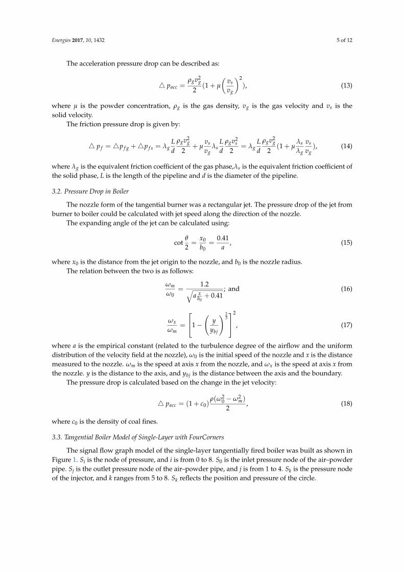
3.2. Pressure Drop in Boiler

The nozzle form of the tangential burner was a rectangular jet. The pressure drop of the jet fromburner to boiler could be calculated with jet speed along the direction of the nozzle.

The expanding angle of the jet can be calculated using:

cotθ

2=

x0

b0=

0.41a

, (15)

where x0 is the distance from the jet origin to the nozzle, and b0 is the nozzle radius.The relation between the two is as follows:

ωm

ω0=

1.2√a x

b0+ 0.41

; and (16)

ωx

ωm=

1−(

yybj

) 232

, (17)

where a is the empirical constant (related to the turbulence degree of the airflow and the uniformdistribution of the velocity field at the nozzle), ω0 is the initial speed of the nozzle and x is the distancemeasured to the nozzle. ωm is the speed at axis x from the nozzle, and ωx is the speed at axis x fromthe nozzle. y is the distance to the axis, and ybj is the distance between the axis and the boundary.

The pressure drop is calculated based on the change in the jet velocity:

4 pacc = (1 + c0)ρ(ω2

0 −ω2m)

2, (18)

where c0 is the density of coal fines.

3.3. Tangential Boiler Model of Single-Layer with FourCorners

The signal flow graph model of the single-layer tangentially fired boiler was built as shown inFigure 1. Si is the node of pressure, and i is from 0 to 8. S0 is the inlet pressure node of the air–powderpipe. Sj is the outlet pressure node of the air–powder pipe, and j is from 1 to 4. Sk is the pressure nodeof the injector, and k ranges from 5 to 8. Sk reflects the position and pressure of the circle.

Energies 2017, 10, 1432 6 of 12Energies 2017, 10, 1432 6 of 12

0S

0S

0S

0S1S 2S

3S4S

5S

6S

7S

8S

Figure 1. Model of the single-layer tangentially fired boiler.

Table 1 shows the structure and parameters of the 350 MW supercritical coal-fired units. Figure 2 is the hypothetical tangential structure for theoretical calculation.

Table 1. Parameters of the boiler structure.

Parameter Value Parameter Value Parameter ValueWidth of boiler 14.904 m Length of boiler 14.094 m Height of boiler 61.900 m

Number of burner layers

5 Number of

secondary air layers

6 Number of over-fire

air layers 2

Elevation of the top burner

27.402 m Elevation of the lowest burner

20.566 m

Internal diameter of pulverized coal

nozzle 0.51 m

External diameter of pulverized coal

nozzle 0.53 m

#1

#2 #3

#4

1.546

14.904

14.094

Figure 2. Hypothetical tangential structure for theoretical calculation.

On the simulation platform STS (Simulation Training System), which was designed independently, algorithms were designed to calculate the node pressure, the pressure drop of the air-powder pipeline and the jet flow. Figure 3 shows the module distribution and connection relationship in STS.

Figure 1. Model of the single-layer tangentially fired boiler.

Table 1 shows the structure and parameters of the 350 MW supercritical coal-fired units. Figure 2is the hypothetical tangential structure for theoretical calculation.

Table 1. Parameters of the boiler structure.

Parameter Value Parameter Value Parameter Value

Width of boiler 14.904 m Length of boiler 14.094 m Height of boiler 61.900 m

Number ofburner layers 5 Number of

secondary air layers 6 Number ofover-fire air layers 2

Elevation of thetop burner 27.402 m Elevation of the

lowest burner 20.566 m

Internal diameterof pulverized

coal nozzle0.51 m

External diameter ofpulverized coal

nozzle0.53 m

Energies 2017, 10, 1432 6 of 12

0S

0S

0S

0S1S 2S

3S4S

5S

6S

7S

8S

Figure 1. Model of the single-layer tangentially fired boiler.

Table 1 shows the structure and parameters of the 350 MW supercritical coal-fired units. Figure 2 is the hypothetical tangential structure for theoretical calculation.

Table 1. Parameters of the boiler structure.

Parameter Value Parameter Value Parameter ValueWidth of boiler 14.904 m Length of boiler 14.094 m Height of boiler 61.900 m

Number of burner layers

5 Number of

secondary air layers

6 Number of over-fire

air layers 2

Elevation of the top burner

27.402 m Elevation of the lowest burner

20.566 m

Internal diameter of pulverized coal

nozzle 0.51 m

External diameter of pulverized coal

nozzle 0.53 m

#1

#2 #3

#4

1.546

14.904

14.094

Figure 2. Hypothetical tangential structure for theoretical calculation.

On the simulation platform STS (Simulation Training System), which was designed independently, algorithms were designed to calculate the node pressure, the pressure drop of the air-powder pipeline and the jet flow. Figure 3 shows the module distribution and connection relationship in STS.

Figure 2. Hypothetical tangential structure for theoretical calculation.

On the simulation platform STS (Simulation Training System), which was designed independently,algorithms were designed to calculate the node pressure, the pressure drop of the air-powder pipelineand the jet flow. Figure 3 shows the module distribution and connection relationship in STS.

Energies 2017, 10, 1432 7 of 12Energies 2017, 10, 1432 7 of 12

Figure 3. Simulation model of the single-layer tangentially fired boiler.

On the simulation platform, the response curves of key parameters with different inputs and external disturbance were studied, as shown in Figure 4.

(a-1) S0 (a-2) S1, S2, S3, S4 (a-3) S5, S6, S7, S8

(b-1) S0 (b-2) S1 (b-3) S2, S3, S4 (b-4) S5, S6, S7, S8

(c-1) S0 (c-2) S1, S3 (c-3) S2, S4 (c-4) S5, S6, S7, S8

(d-1) S0 (d-2) S1, S3 (d-3) S2, S4 (d-4) S5, S6, S7, S8

Figure 4. Response curves of the (a) powder entrance with pressure disturbance; (b) powder entrance with pressure disturbance when powder pipe 1 was blocked; (c) powder entrance with pressure disturbance when powder pipes 1 and 3 were blocked; and (d) powder exit with pressure disturbance when powder pipes 1 and 3 were blocked.

0 50 100 150 200100.2

100.4

100.6

100.8

101

101.2

0 50 100 150 200

99.9

100

100.1

100.2

100.3

0 50 100 150 20099.35

99.36

99.37

99.38

99.39

99.4

0 100 200100.2

100.4

100.6

100.8

101

101.2

0 100 20099.38

99.4

99.42

99.44

99.46

0 100 200

99.9

100

100.1

100.2

100.3

0 100 20099.325

99.33

99.335

99.34

99.345

99.35

99.355

99.36

0 50 100 150 200100.4

100.6

100.8

101

101.2

101.4

0 50 100 150 20099.38

99.4

99.42

99.44

99.46

0 50 100 150 200

99.9

100

100.1

100.2

100.3

0 50 100 150 20099.32

99.325

99.33

99.335

99.34

99.345

99.35

99.355

0 100 200100.5

100.6

100.7

100.8

100.9

101

0 100 20099.4

99.405

99.41

99.415

99.42

99.425

99.43

99.435

0 100 20099.95

100

100.05

100.1

0 100 20099.328

99.33

99.332

99.334

99.336

Figure 3. Simulation model of the single-layer tangentially fired boiler.

On the simulation platform, the response curves of key parameters with different inputs andexternal disturbance were studied, as shown in Figure 4.

Energies 2017, 10, 1432 7 of 12

Figure 3. Simulation model of the single-layer tangentially fired boiler.

On the simulation platform, the response curves of key parameters with different inputs and external disturbance were studied, as shown in Figure 4.

(a-1) S0 (a-2) S1, S2, S3, S4 (a-3) S5, S6, S7, S8

(b-1) S0 (b-2) S1 (b-3) S2, S3, S4 (b-4) S5, S6, S7, S8

(c-1) S0 (c-2) S1, S3 (c-3) S2, S4 (c-4) S5, S6, S7, S8

(d-1) S0 (d-2) S1, S3 (d-3) S2, S4 (d-4) S5, S6, S7, S8

Figure 4. Response curves of the (a) powder entrance with pressure disturbance; (b) powder entrance with pressure disturbance when powder pipe 1 was blocked; (c) powder entrance with pressure disturbance when powder pipes 1 and 3 were blocked; and (d) powder exit with pressure disturbance when powder pipes 1 and 3 were blocked.

0 50 100 150 200100.2

100.4

100.6

100.8

101

101.2

0 50 100 150 200

99.9

100

100.1

100.2

100.3

0 50 100 150 20099.35

99.36

99.37

99.38

99.39

99.4

0 100 200100.2

100.4

100.6

100.8

101

101.2

0 100 20099.38

99.4

99.42

99.44

99.46

0 100 200

99.9

100

100.1

100.2

100.3

0 100 20099.325

99.33

99.335

99.34

99.345

99.35

99.355

99.36

0 50 100 150 200100.4

100.6

100.8

101

101.2

101.4

0 50 100 150 20099.38

99.4

99.42

99.44

99.46

0 50 100 150 200

99.9

100

100.1

100.2

100.3

0 50 100 150 20099.32

99.325

99.33

99.335

99.34

99.345

99.35

99.355

0 100 200100.5

100.6

100.7

100.8

100.9

101

0 100 20099.4

99.405

99.41

99.415

99.42

99.425

99.43

99.435

0 100 20099.95

100

100.05

100.1

0 100 20099.328

99.33

99.332

99.334

99.336

Figure 4. Response curves of the (a) powder entrance with pressure disturbance; (b) powder entrancewith pressure disturbance when powder pipe 1 was blocked; (c) powder entrance with pressuredisturbance when powder pipes 1 and 3 were blocked; and (d) powder exit with pressure disturbancewhen powder pipes 1 and 3 were blocked.

Energies 2017, 10, 1432 8 of 12

In the subfigures, the ordinate is absolute pressure and the unit is KPa. By changing the inletpressure disturbance of the air-powder pipe, the response curves of the air-powder pipe outlet pressureand the injector pressure were studied.

It can be seen from the subfigures that the position and pressure of the tangential circle variedwith the pressure of the separator outlet of the coal grinding machine (and the inlet of the air-powderpipeline). When the air-powder pipelines were blocked, the amplitude of the pressure varied.According to the curve in Figure 4d, on the same branch of the fluid network, the pressure changeof the downstream node lagged behind the front node. The lag time was adjusted by ci in the nodecalculation process.

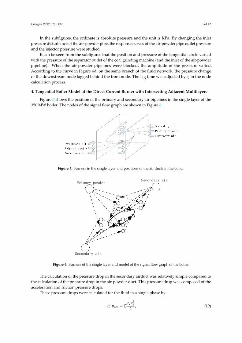
4. Tangential Boiler Model of the Direct-Current Burner with Intersecting Adjacent Multilayers

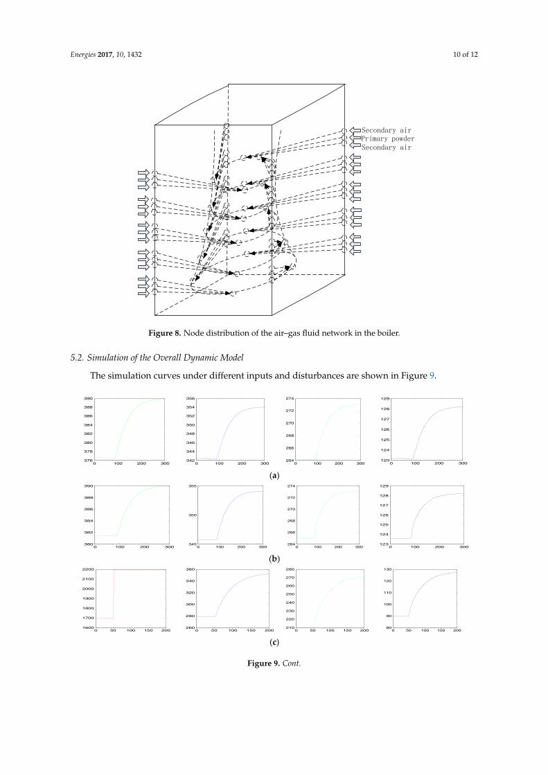
Figure 5 shows the position of the primary and secondary air pipelines in the single layer of the350 MW boiler. The nodes of the signal flow graph are shown in Figure 6.

Energies 2017, 10, 1432 8 of 12

In the subfigures, the ordinate is absolute pressure and the unit is KPa. By changing the inlet pressure disturbance of the air-powder pipe, the response curves of the air-powder pipe outlet pressure and the injector pressure were studied.

It can be seen from the subfigures that the position and pressure of the tangential circle varied with the pressure of the separator outlet of the coal grinding machine (and the inlet of the air-powder pipeline). When the air-powder pipelines were blocked, the amplitude of the pressure varied. According to the curve in Figure 4d, on the same branch of the fluid network, the pressure change of the downstream node lagged behind the front node. The lag time was adjusted by ci in the node calculation process.

4. Tangential Boiler Model of the Direct-Current Burner with Intersecting Adjacent Multilayers

Figure 5 shows the position of the primary and secondary air pipelines in the single layer of the 350 MW boiler. The nodes of the signal flow graph are shown in Figure 6.

Figure 5. Burners in the single layer and positions of the air ducts in the boiler.

Secondary airPrimary powder

Secondary air

Figure 6. Burners of the single layer and model of the signal flow graph of the boiler.

The calculation of the pressure drop in the secondary airduct was relatively simple compared to the calculation of the pressure drop in the air-powder duct. This pressure drop was composed of the acceleration and friction pressure drops.

These pressure drops were calculated for the fluid in a single phase by:

2

2g g

accpρ υ

ζ= , (19)

Figure 5. Burners in the single layer and positions of the air ducts in the boiler.

Energies 2017, 10, 1432 8 of 12

In the subfigures, the ordinate is absolute pressure and the unit is KPa. By changing the inlet pressure disturbance of the air-powder pipe, the response curves of the air-powder pipe outlet pressure and the injector pressure were studied.

It can be seen from the subfigures that the position and pressure of the tangential circle varied with the pressure of the separator outlet of the coal grinding machine (and the inlet of the air-powder pipeline). When the air-powder pipelines were blocked, the amplitude of the pressure varied. According to the curve in Figure 4d, on the same branch of the fluid network, the pressure change of the downstream node lagged behind the front node. The lag time was adjusted by ci in the node calculation process.

4. Tangential Boiler Model of the Direct-Current Burner with Intersecting Adjacent Multilayers

Figure 5 shows the position of the primary and secondary air pipelines in the single layer of the 350 MW boiler. The nodes of the signal flow graph are shown in Figure 6.

Figure 5. Burners in the single layer and positions of the air ducts in the boiler.

Secondary airPrimary powder

Secondary air

Figure 6. Burners of the single layer and model of the signal flow graph of the boiler.

The calculation of the pressure drop in the secondary airduct was relatively simple compared to the calculation of the pressure drop in the air-powder duct. This pressure drop was composed of the acceleration and friction pressure drops.

These pressure drops were calculated for the fluid in a single phase by:

2

2g g

accpρ υ

ζ= , (19)

Figure 6. Burners of the single layer and model of the signal flow graph of the boiler.

The calculation of the pressure drop in the secondary airduct was relatively simple compared tothe calculation of the pressure drop in the air-powder duct. This pressure drop was composed of theacceleration and friction pressure drops.

These pressure drops were calculated for the fluid in a single phase by:

4 pacc = ζρgυ2

g

2, (19)

Energies 2017, 10, 1432 9 of 12

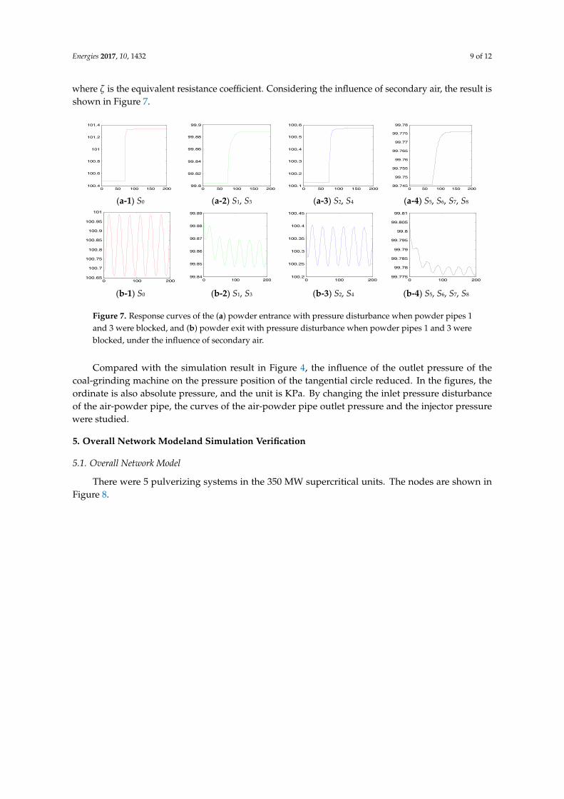
where ζ is the equivalent resistance coefficient. Considering the influence of secondary air, the result isshown in Figure 7.

Energies 2017, 10, 1432 9 of 12

where ζ is the equivalent resistance coefficient. Considering the influence of secondary air, the result is shown in Figure 7.

(a-1) S0 (a-2) S1, S3 (a-3) S2, S4 (a-4) S5, S6, S7, S8

(b-1) S0 (b-2) S1, S3 (b-3) S2, S4 (b-4) S5, S6, S7, S8

Figure 7. Response curves of the (a) powder entrance with pressure disturbance when powder pipes 1 and 3 were blocked, and (b) powder exit with pressure disturbance when powder pipes 1 and 3 were blocked, under the influence of secondary air.

Compared with the simulation result in Figure 4, the influence of the outlet pressure of the coal-grinding machine on the pressure position of the tangential circle reduced. In the figures, the ordinate is also absolute pressure, and the unit is KPa. By changing the inlet pressure disturbance of the air-powder pipe, the curves of the air-powder pipe outlet pressure and the injector pressure were studied.

5. Overall Network Modeland Simulation Verification

5.1. Overall Network Model

There were 5 pulverizing systems in the 350 MW supercritical units. The nodes are shown in Figure 8.

0 50 100 150 200100.4

100.6

100.8

101

101.2

101.4

0 50 100 150 20099.8

99.82

99.84

99.86

99.88

99.9

0 50 100 150 200100.1

100.2

100.3

100.4

100.5

100.6

0 50 100 150 20099.745

99.75

99.755

99.76

99.765

99.77

99.775

99.78

0 100 200100.65

100.7

100.75

100.8

100.85

100.9

100.95

101

0 100 20099.84

99.85

99.86

99.87

99.88

99.89

0 100 200100.2

100.25

100.3

100.35

100.4

100.45

0 100 20099.775

99.78

99.785

99.79

99.795

99.8

99.805

99.81

Figure 7. Response curves of the (a) powder entrance with pressure disturbance when powder pipes 1and 3 were blocked, and (b) powder exit with pressure disturbance when powder pipes 1 and 3 wereblocked, under the influence of secondary air.

Compared with the simulation result in Figure 4, the influence of the outlet pressure of thecoal-grinding machine on the pressure position of the tangential circle reduced. In the figures, theordinate is also absolute pressure, and the unit is KPa. By changing the inlet pressure disturbanceof the air-powder pipe, the curves of the air-powder pipe outlet pressure and the injector pressurewere studied.

5. Overall Network Modeland Simulation Verification

5.1. Overall Network Model

There were 5 pulverizing systems in the 350 MW supercritical units. The nodes are shown inFigure 8.

Energies 2017, 10, 1432 10 of 12Energies 2017, 10, 1432 10 of 12

Secondary airPrimary powderSecondary air

Figure 8.Node distribution of the air–gas fluid network in the boiler.

5.2. Simulation of the Overall Dynamic Model

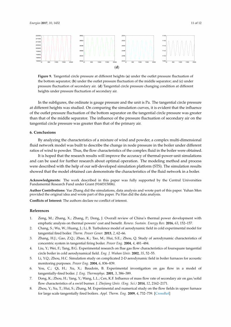
The simulation curves under different inputs and disturbances are shown in Figure 9.

(a)

(b)

(c)

0 100 200 300376

378

380

382

384

386

388

390

0 100 200 300342

344

346

348

350

352

354

356

0 100 200 300264

266

268

270

272

274

0 100 200 300123

124

125

126

127

128

129

0 100 200 300380

382

384

386

388

390

0 100 200 300345

350

355

0 100 200 300264

266

268

270

272

274

0 100 200 300123

124

125

126

127

128

129

0 50 100 150 2001600

1700

1800

1900

2000

2100

2200

0 50 100 150 200260

280

300

320

340

360

0 50 100 150 200210

220

230

240

250

260

270

280

0 50 100 150 20080

90

100

110

120

130

Figure 8. Node distribution of the air–gas fluid network in the boiler.

5.2. Simulation of the Overall Dynamic Model

The simulation curves under different inputs and disturbances are shown in Figure 9.

Energies 2017, 10, 1432 10 of 12

Secondary airPrimary powderSecondary air

Figure 8.Node distribution of the air–gas fluid network in the boiler.

5.2. Simulation of the Overall Dynamic Model

The simulation curves under different inputs and disturbances are shown in Figure 9.

(a)

(b)

(c)

0 100 200 300376

378

380

382

384

386

388

390

0 100 200 300342

344

346

348

350

352

354

356

0 100 200 300264

266

268

270

272

274

0 100 200 300123

124

125

126

127

128

129

0 100 200 300380

382

384

386

388

390

0 100 200 300345

350

355

0 100 200 300264

266

268

270

272

274

0 100 200 300123

124

125

126

127

128

129

0 50 100 150 2001600

1700

1800

1900

2000

2100

2200

0 50 100 150 200260

280

300

320

340

360

0 50 100 150 200210

220

230

240

250

260

270

280

0 50 100 150 20080

90

100

110

120

130

Figure 9. Cont.

Energies 2017, 10, 1432 11 of 12Energies 2017, 10, 1432 11 of 12

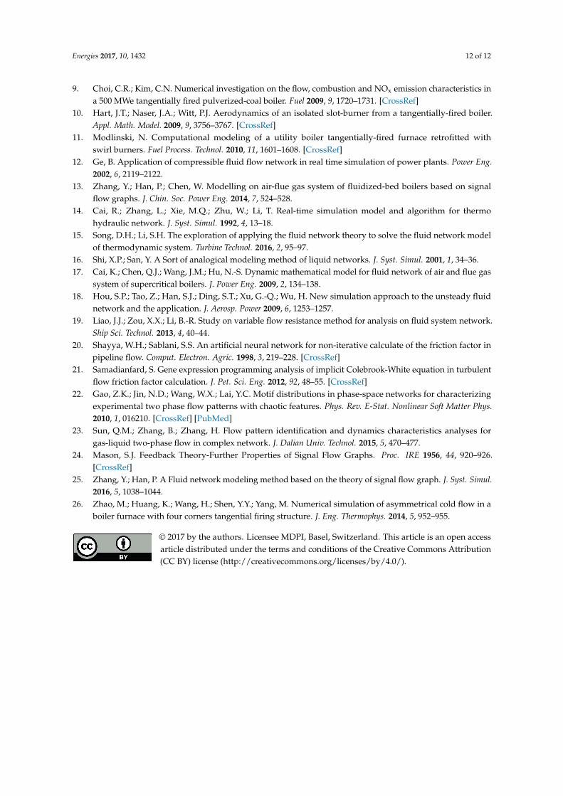
(d)

Figure 9. Tangential circle pressure at different heights (a) under the outlet pressure fluctuation of the bottom separator; (b) under the outlet pressure fluctuation of the middle separator; and (c) under pressure fluctuation of secondary air. (d) Tangential circle pressure changing condition at different heights under pressure fluctuation of secondary air.

In the subfigures, the ordinate is gauge pressure and the unit is Pa. The tangential circle pressure at different heights was studied. On comparing the simulation curves, it is evident that the influence of the outlet pressure fluctuation of the bottom separator on the tangential circle pressure was greater than that of the middle separator. The influence of the pressure fluctuation of secondary air on the tangential circle pressure was greater than that of the primary air.

6. Conclusions

By analyzing the characteristics of a mixture of wind and powder, a complex multi-dimensional fluid network model was built to describe the change in node pressure in the boiler under different ratios of wind to powder. Thus, the flow characteristics of the complex fluid in the boiler were obtained.

It is hoped that the research results will improve the accuracy of thermal-power-unit simulations and can be used for further research about optimal operation. The modeling method and process were described with the help of our self-developed simulation platform (STS). The simulation results showed that the model obtained can demonstrate the characteristics of the fluid network in a boiler.

Acknowledgments: The work described in this paper was fully supported by the Central Universities Fundamental Research Fund under Grant (9160315006).

Author Contributions: Yue Zhang did the simulations, data analysis and wrote part of this paper. Yuhan Men provided the original idea and wrote part of this paper. Pu Han did the data analysis.

Conflicts of Interest: The authors declare no conflict of interest.

References

1. Zeng, M.; Zhang, X.; Zhang, P.; Dong, J. Overall review of China’s thermal power development with emphatic analysis on thermal powers’ cost and benefit. Renew. Sustain. Energy Rev. 2016, 63, 152–157.

2. Chang, S.; Wu, W.; Huang, J.; Li, B. Turbulence model of aerodynamic field in cold experimental model for tangential fired boiler. Therm. Power Gener. 2013, 2, 62–66.

3. Zhang, H.J.; Gao, Z.Q.; Zhao, K.; Tao, M.; Hui, S.E.; Zhou, Q. Study of aerodynamic characteristics of concentric system in tangential firing boiler. Power Eng. 2004, 4, 481–484.

4. Liu, Y.; Wei, F.; Tang, B.G. Experimental research on flue gas flow characteristics of foursquare tangential circle boiler in cold aerodynamical field. Eng. J. Wuhan Univ. 2002, 35, 52–55.

5. Li, Y.Q.; Zhou, H.C. Simulation study on complicated 2-D aerodynamic field in boiler furnaces for acoustic monitoring purposes. Power Eng. 2004, 6, 836–839.

6. You, C.; Qi, H.; Xu, X; Baudoin B. Experimental investigation on gas flow in a model of tangentially-fired boiler. J. Eng. Thermophys. 2001, 3, 386–389.

7. Dong, K.; Zhou, H.; Yang, Y.; Wang, L.L.; Cen, K.F. Influence of mass flow rate of secondary air on gas/solid flow characteristics of a swirl burner. J. Zhejiang Univ. (Eng. Sci.) 2014, 12, 2162–2171.

8. Zhou, Y.; Xu, T.; Hui, S.; Zhang, M. Experimental and numerical study on the flow fields in upper furnace for large scale tangentially fired boilers. Appl. Therm. Eng. 2009, 4, 732–739.

0 50 100 150 2001800

1850

1900

1950

2000

2050

2100

2150

2200

0 50 100 150 200352

354

356

358

360

362

0 50 100 150 200244

246

248

250

252

254

0 50 100 150 200108

110

112

114

116

118

Figure 9. Tangential circle pressure at different heights (a) under the outlet pressure fluctuation ofthe bottom separator; (b) under the outlet pressure fluctuation of the middle separator; and (c) underpressure fluctuation of secondary air. (d) Tangential circle pressure changing condition at differentheights under pressure fluctuation of secondary air.

In the subfigures, the ordinate is gauge pressure and the unit is Pa. The tangential circle pressureat different heights was studied. On comparing the simulation curves, it is evident that the influenceof the outlet pressure fluctuation of the bottom separator on the tangential circle pressure was greaterthan that of the middle separator. The influence of the pressure fluctuation of secondary air on thetangential circle pressure was greater than that of the primary air.

6. Conclusions

By analyzing the characteristics of a mixture of wind and powder, a complex multi-dimensionalfluid network model was built to describe the change in node pressure in the boiler under differentratios of wind to powder. Thus, the flow characteristics of the complex fluid in the boiler were obtained.

It is hoped that the research results will improve the accuracy of thermal-power-unit simulationsand can be used for further research about optimal operation. The modeling method and processwere described with the help of our self-developed simulation platform (STS). The simulation resultsshowed that the model obtained can demonstrate the characteristics of the fluid network in a boiler.

Acknowledgments: The work described in this paper was fully supported by the Central UniversitiesFundamental Research Fund under Grant (9160315006).

Author Contributions: Yue Zhang did the simulations, data analysis and wrote part of this paper. Yuhan Menprovided the original idea and wrote part of this paper. Pu Han did the data analysis.

Conflicts of Interest: The authors declare no conflict of interest.

References

1. Zeng, M.; Zhang, X.; Zhang, P.; Dong, J. Overall review of China’s thermal power development withemphatic analysis on thermal powers’ cost and benefit. Renew. Sustain. Energy Rev. 2016, 63, 152–157.

2. Chang, S.; Wu, W.; Huang, J.; Li, B. Turbulence model of aerodynamic field in cold experimental model fortangential fired boiler. Therm. Power Gener. 2013, 2, 62–66.

3. Zhang, H.J.; Gao, Z.Q.; Zhao, K.; Tao, M.; Hui, S.E.; Zhou, Q. Study of aerodynamic characteristics ofconcentric system in tangential firing boiler. Power Eng. 2004, 4, 481–484.

4. Liu, Y.; Wei, F.; Tang, B.G. Experimental research on flue gas flow characteristics of foursquare tangentialcircle boiler in cold aerodynamical field. Eng. J. Wuhan Univ. 2002, 35, 52–55.

5. Li, Y.Q.; Zhou, H.C. Simulation study on complicated 2-D aerodynamic field in boiler furnaces for acousticmonitoring purposes. Power Eng. 2004, 6, 836–839.

6. You, C.; Qi, H.; Xu, X.; Baudoin, B. Experimental investigation on gas flow in a model oftangentially-fired boiler. J. Eng. Thermophys. 2001, 3, 386–389.

7. Dong, K.; Zhou, H.; Yang, Y.; Wang, L.L.; Cen, K.F. Influence of mass flow rate of secondary air on gas/solidflow characteristics of a swirl burner. J. Zhejiang Univ. (Eng. Sci.) 2014, 12, 2162–2171.

8. Zhou, Y.; Xu, T.; Hui, S.; Zhang, M. Experimental and numerical study on the flow fields in upper furnacefor large scale tangentially fired boilers. Appl. Therm. Eng. 2009, 4, 732–739. [CrossRef]

Energies 2017, 10, 1432 12 of 12

9. Choi, C.R.; Kim, C.N. Numerical investigation on the flow, combustion and NOx emission characteristics ina 500 MWe tangentially fired pulverized-coal boiler. Fuel 2009, 9, 1720–1731. [CrossRef]

10. Hart, J.T.; Naser, J.A.; Witt, P.J. Aerodynamics of an isolated slot-burner from a tangentially-fired boiler.Appl. Math. Model. 2009, 9, 3756–3767. [CrossRef]

11. Modlinski, N. Computational modeling of a utility boiler tangentially-fired furnace retrofitted withswirl burners. Fuel Process. Technol. 2010, 11, 1601–1608. [CrossRef]

12. Ge, B. Application of compressible fluid flow network in real time simulation of power plants. Power Eng.2002, 6, 2119–2122.

13. Zhang, Y.; Han, P.; Chen, W. Modelling on air-flue gas system of fluidized-bed boilers based on signalflow graphs. J. Chin. Soc. Power Eng. 2014, 7, 524–528.

14. Cai, R.; Zhang, L.; Xie, M.Q.; Zhu, W.; Li, T. Real-time simulation model and algorithm for thermohydraulic network. J. Syst. Simul. 1992, 4, 13–18.

15. Song, D.H.; Li, S.H. The exploration of applying the fluid network theory to solve the fluid network modelof thermodynamic system. Turbine Technol. 2016, 2, 95–97.

16. Shi, X.P.; San, Y. A Sort of analogical modeling method of liquid networks. J. Syst. Simul. 2001, 1, 34–36.17. Cai, K.; Chen, Q.J.; Wang, J.M.; Hu, N.-S. Dynamic mathematical model for fluid network of air and flue gas

system of supercritical boilers. J. Power Eng. 2009, 2, 134–138.18. Hou, S.P.; Tao, Z.; Han, S.J.; Ding, S.T.; Xu, G.-Q.; Wu, H. New simulation approach to the unsteady fluid

network and the application. J. Aerosp. Power 2009, 6, 1253–1257.19. Liao, J.J.; Zou, X.X.; Li, B.-R. Study on variable flow resistance method for analysis on fluid system network.

Ship Sci. Technol. 2013, 4, 40–44.20. Shayya, W.H.; Sablani, S.S. An artificial neural network for non-iterative calculate of the friction factor in

pipeline flow. Comput. Electron. Agric. 1998, 3, 219–228. [CrossRef]21. Samadianfard, S. Gene expression programming analysis of implicit Colebrook-White equation in turbulent

flow friction factor calculation. J. Pet. Sci. Eng. 2012, 92, 48–55. [CrossRef]22. Gao, Z.K.; Jin, N.D.; Wang, W.X.; Lai, Y.C. Motif distributions in phase-space networks for characterizing

experimental two phase flow patterns with chaotic features. Phys. Rev. E-Stat. Nonlinear Soft Matter Phys.2010, 1, 016210. [CrossRef] [PubMed]

23. Sun, Q.M.; Zhang, B.; Zhang, H. Flow pattern identification and dynamics characteristics analyses forgas-liquid two-phase flow in complex network. J. Dalian Univ. Technol. 2015, 5, 470–477.

24. Mason, S.J. Feedback Theory-Further Properties of Signal Flow Graphs. Proc. IRE 1956, 44, 920–926.[CrossRef]

25. Zhang, Y.; Han, P. A Fluid network modeling method based on the theory of signal flow graph. J. Syst. Simul.2016, 5, 1038–1044.

26. Zhao, M.; Huang, K.; Wang, H.; Shen, Y.Y.; Yang, M. Numerical simulation of asymmetrical cold flow in aboiler furnace with four corners tangential firing structure. J. Eng. Thermophys. 2014, 5, 952–955.

© 2017 by the authors. Licensee MDPI, Basel, Switzerland. This article is an open accessarticle distributed under the terms and conditions of the Creative Commons Attribution(CC BY) license (http://creativecommons.org/licenses/by/4.0/).