1

MODELING AND PLANNING FOR IMPACTS OF COASTAL FLOODING AND SEA LEVEL RISE ON CURRENT AND FUTURE DEVELOPMENT IN ST. JOHNS COUNTY,

FLORIDA

By

ADAM HAMMOND CARR

A THESIS PRESENTED TO THE GRADUATE SCHOOL OF THE UNIVERSITY OF FLORIDA IN PARTIAL FULFILLMENT

OF THE REQUIREMENTS FOR THE DEGREE OF MASTER OF URBAN AND REGIONAL PLANNING

UNIVERSITY OF FLORIDA

2018

2

© 2018 Adam Hammond Carr

3

For my parents, David and Peggy

4

ACKNOWLEDGMENTS

Many people have helped me over the course of my studies here at UF and,

more broadly, over the course of my life. My parents have been extremely supportive

and have offered important guidance to me throughout my life. From an early age they

instilled in me a respect for the natural world and a desire to protect. This mindset has

guided me through all of my ventures.

I want to thank all of my colleagues at the GeoPlan Center, especially Crystal

Goodison and Lex Thomas, who offered me a terrific environment to grow my GIS skills

and knowledge. I hope to carry the character and quality of this work and learning

environment with me in my future endeavors.

I also want to thank all of my professors at UF, especially Dr. Paul Zwick and Dr.

Katherine Frank, who helped me work through my research and studies. They have

fostered in me a strong sense of how planners can have a positive impact on the world

and the importance of thinking critically about planning problems.

Finally, I want to recognize the friends I have made during my time at UF.

Already I have seen them start their careers and work to improve the human

environments that we live in. We have a wonderful opportunity to use our knowledge

and education to work towards the greater good of the public and the planet. Despite

the challenges we may face, I’m confident we will overcome challenges we face at a

variety of levels. I look forward to continuing to consider difficult problems, using data

and sound analysis to make informed decisions.

5

TABLE OF CONTENTS

page

ACKNOWLEDGMENTS .................................................................................................. 4

LIST OF TABLES ............................................................................................................ 7

LIST OF FIGURES .......................................................................................................... 8

LIST OF ABBREVIATIONS ........................................................................................... 10

ABSTRACT……………………………………………………………………………….........11 CHAPTER

1 INTRODUCTION .................................................................................................... 13

Sea Level Rise and Coastal Flooding Threats in Florida ........................................ 13 Future Growth in St. Johns County and Potential Impacts ..................................... 15

Research Outcomes ............................................................................................... 20

2 LITERATURE REVIEW .......................................................................................... 22

Sea Level Rise Forecasting ................................................................................... 22 Modeling Coastal Flooding ..................................................................................... 25

Estimating Impacts of Coastal Flooding Events ..................................................... 31

3 METHODOLOGY ................................................................................................... 36

Data Acquisition ..................................................................................................... 38 Hazus-MH Model Descriptions ............................................................................... 43 Current Development Economic Impact Analysis................................................... 45

Future Development Economic Impact Analysis .................................................... 47

4 COASTAL FLOODING AND SEA LEVEL RISE RESULTS ................................... 49

5 ECONOMIC IMPACT RESULTS ............................................................................ 54

Current Development Impact Results ..................................................................... 54 Future Development Impact Results ...................................................................... 55

6 DISCUSSION AND CONCLUSION ........................................................................ 58

Coastal Flooding from Base 100-Year Storm and Impacts .................................... 58 Coastal Flooding from 100-Year Storms with Extra Sea Level Rise and Impacts .. 62 Coastal Flooding Impacts on Future Development................................................. 66

Additional Considerations ....................................................................................... 70

6

Limitations .............................................................................................................. 74 Suggestions for Future Research ........................................................................... 75

Concluding Thoughts ............................................................................................. 77 APPENDIX

A HAZUS-MH COASTAL FLOODING MODEL WORKFLOW .................................. 79

B ECONOMIC IMPACT ANALYSIS WORKFLOW .................................................... 82

C COASTAL FLOODING MODEL OUTPUT MAPS .................................................. 91

REFERENCES ............................................................................................................ 107

BIOGRAPHICAL SKETCH .......................................................................................... 111

7

LIST OF TABLES Table page 2-1 General Descriptions of Coastal Flooding Models ………………………………. 26 2-2 National Averages for Full Replacement Cost Models of Various Building

Occupancies ……………...…………………………………………………………. 34 4-1 Flood Statistics for Coastal Flooding Scenarios Incorporating Varying

Amounts of Sea Level Rise in St. Johns County ...……………………….……… 49 5-1 Current Economic Impact Results ……………………………………………….... 55 5-2 Future Economic Impact Results ………………………………………………….. 57 5-3 Future Economic Impact Results Continued …….……………………………….. 57

8

LIST OF FIGURES Figure page 1-1 Florida 2070: Currently Developed Areas in St. Johns County – 2010

Base Scenario …………………………………………………………..………….. 17 1-2 Florida 2070: Currently Developed Areas with Future Development in

St. Johns County – 2070 Trend Scenario ……………………………………..… 18 1-3 Florida 2070: Currently Developed Areas with Future Development in

St. Johns County – 2070 Alternative Scenario ….………………………….….... 19 2-1 Mean Sea Level Trend – Gauge Station 8720218 Mayport, Florida ………..… 23 3-1 Generalized Research Process Steps …………………………………….……… 37 3-2 General Hazus-MH Coastal Flood Model Workflow ……………………….……. 44 3-3 General Parcel-Level Economic Impact Analysis Workflow ……………………. 46 4-1 Hazus Coastal Flooding Output – Base Flooding Scenario in the

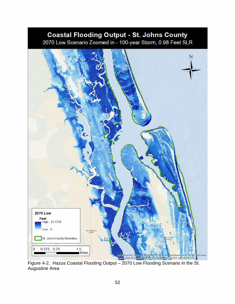
St. Augustine Area ...……………………......………………………………………. 51 4-2 Hazus Coastal Flooding Output – 2070 Low Flooding Scenario in the

St. Augustine Area ………………………………………………………………....... 52 4-3 Hazus Coastal Flooding Output – 2070 High Flooding Scenario in the

St. Augustine Area …..……………………………………………………………..... 53 6-1 Hazus Coastal Flooding Output – Base Flooding Scenario for St. Johns

County…………………………………………………………………………………..60 6-2 Hazus Coastal Flooding Output – Base Flooding Scenario in the

St. Augustine Area …………...…………………………………………………….... 61 6-3 Hazus Coastal Flooding Output – 2070 VLM Flooding Scenario for

St. Johns County ………………………………………………………………..…… 64 6-4 Hazus Coastal Flooding Output – 2070 Extreme Flooding Scenario for

St. Johns County ..…………………………………………………………………… 65 6-5 Hazus Coastal Flooding Output – 2070 VLM Flooding Scenario, Impact

on Future Development Near St. Augustine .…….……..………………………... 68 6-6 Hazus Coastal Flooding Output – 2070 Extreme Flooding Scenario,

Impact on Future Development Near St. Augustine ……………………………... 69

9

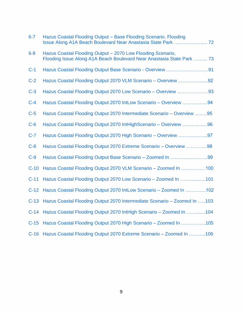
6-7 Hazus Coastal Flooding Output – Base Flooding Scenario, Flooding

Issue Along A1A Beach Boulevard Near Anastasia State Park ….…………...... 72 6-8 Hazus Coastal Flooding Output – 2070 Low Flooding Scenario,

Flooding Issue Along A1A Beach Boulevard Near Anastasia State Park ……... 73 C-1 Hazus Coastal Flooding Output Base Scenario - Overview .……………………..91 C-2 Hazus Coastal Flooding Output 2070 VLM Scenario – Overview ..…………......92 C-3 Hazus Coastal Flooding Output 2070 Low Scenario – Overview ..………………93 C-4 Hazus Coastal Flooding Output 2070 IntLow Scenario – Overview .……………94 C-5 Hazus Coastal Flooding Output 2070 Intermediate Scenario – Overview .…….95 C-6 Hazus Coastal Flooding Output 2070 IntHighScenario – Overview .……………96 C-7 Hazus Coastal Flooding Output 2070 High Scenario – Overview .……………...97 C-8 Hazus Coastal Flooding Output 2070 Extreme Scenario – Overview .………....98 C-9 Hazus Coastal Flooding Output Base Scenario – Zoomed In .…………………..99 C-10 Hazus Coastal Flooding Output 2070 VLM Scenario – Zoomed In …...…….…100 C-11 Hazus Coastal Flooding Output 2070 Low Scenario – Zoomed In ……............101 C-12 Hazus Coastal Flooding Output 2070 IntLow Scenario – Zoomed In ………….102 C-13 Hazus Coastal Flooding Output 2070 Intermediate Scenario – Zoomed In …..103 C-14 Hazus Coastal Flooding Output 2070 IntHigh Scenario – Zoomed In …….......104 C-15 Hazus Coastal Flooding Output 2070 High Scenario – Zoomed In …………....105 C-16 Hazus Coastal Flooding Output 2070 Extreme Scenario – Zoomed In …….....106

10

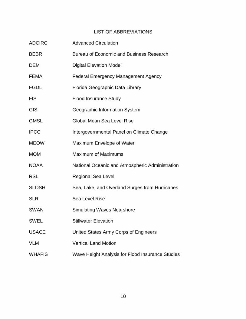
LIST OF ABBREVIATIONS ADCIRC Advanced Circulation BEBR Bureau of Economic and Business Research DEM Digital Elevation Model FEMA Federal Emergency Management Agency FGDL Florida Geographic Data Library FIS Flood Insurance Study GIS Geographic Information System GMSL Global Mean Sea Level Rise IPCC Intergovernmental Panel on Climate Change MEOW Maximum Envelope of Water MOM Maximum of Maximums NOAA National Oceanic and Atmospheric Administration RSL Regional Sea Level SLOSH Sea, Lake, and Overland Surges from Hurricanes SLR Sea Level Rise SWAN Simulating Waves Nearshore SWEL Stillwater Elevation USACE United States Army Corps of Engineers VLM Vertical Land Motion WHAFIS Wave Height Analysis for Flood Insurance Studies

11

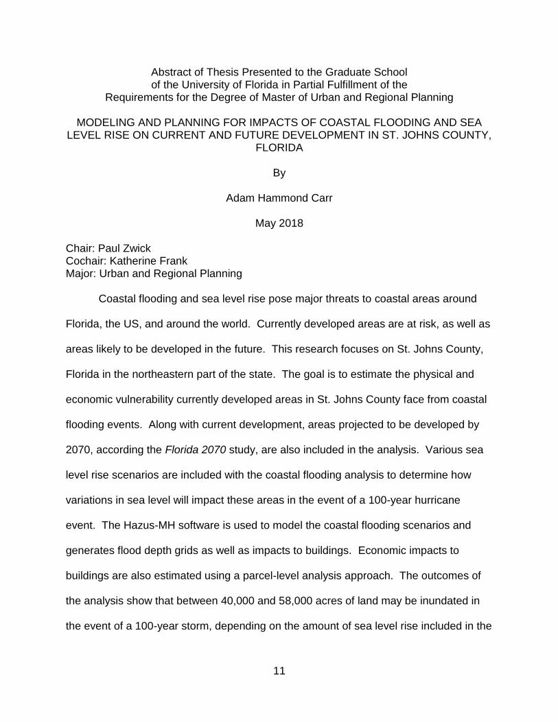
Abstract of Thesis Presented to the Graduate School of the University of Florida in Partial Fulfillment of the

Requirements for the Degree of Master of Urban and Regional Planning

MODELING AND PLANNING FOR IMPACTS OF COASTAL FLOODING AND SEA LEVEL RISE ON CURRENT AND FUTURE DEVELOPMENT IN ST. JOHNS COUNTY,

FLORIDA

By

Adam Hammond Carr

May 2018

Chair: Paul Zwick Cochair: Katherine Frank Major: Urban and Regional Planning Coastal flooding and sea level rise pose major threats to coastal areas around

Florida, the US, and around the world. Currently developed areas are at risk, as well as

areas likely to be developed in the future. This research focuses on St. Johns County,

Florida in the northeastern part of the state. The goal is to estimate the physical and

economic vulnerability currently developed areas in St. Johns County face from coastal

flooding events. Along with current development, areas projected to be developed by

2070, according the Florida 2070 study, are also included in the analysis. Various sea

level rise scenarios are included with the coastal flooding analysis to determine how

variations in sea level will impact these areas in the event of a 100-year hurricane

event. The Hazus-MH software is used to model the coastal flooding scenarios and

generates flood depth grids as well as impacts to buildings. Economic impacts to

buildings are also estimated using a parcel-level analysis approach. The outcomes of

the analysis show that between 40,000 and 58,000 acres of land may be inundated in

the event of a 100-year storm, depending on the amount of sea level rise included in the

12

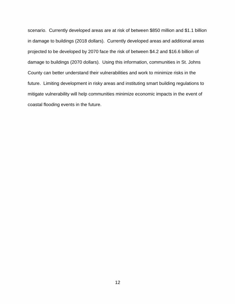
scenario. Currently developed areas are at risk of between $850 million and $1.1 billion

in damage to buildings (2018 dollars). Currently developed areas and additional areas

projected to be developed by 2070 face the risk of between $4.2 and $16.6 billion of

damage to buildings (2070 dollars). Using this information, communities in St. Johns

County can better understand their vulnerabilities and work to minimize risks in the

future. Limiting development in risky areas and instituting smart building regulations to

mitigate vulnerability will help communities minimize economic impacts in the event of

coastal flooding events in the future.

13

CHAPTER 1 INTRODUCTION

Sea Level Rise and Coastal Flooding Threats in Florida

Coastal flooding and sea level rise pose major threats to seaside communities

around the world. Areas with developed coastlines have increased vulnerabilities to

infrastructure, as well as human life, which is at risk of damage or loss due to these

hazards. Florida faces particular vulnerability because large portions of the coastline

have been developed, coastal areas are at or very near sea level, and the peninsula is

exposed to powerful tropical cyclones. Coastal areas are major contributors to Florida’s

real estate and tourism markets, which form big pieces of the state’s economy (Florida

Ocean Alliance, 2013; Bureau of Economic Analysis, 2017; Oxford Economics, 2018;

Trigaux, 2016). In addition, many highly populated cities and areas of cultural

significance can be found on or near the coasts, with eight of Florida’s ten most

populous cities near the coast (Office of Economic and Demographic Research, 2017).

To add to this, Florida’s vulnerabilities are only likely to grow in the future. Over

the next 50 years, it is estimated that about ten million people will move to Florida,

putting the total population around 30 million (Florida Bureau of Economic and Business

Research, 2015; Carr& Zwick, 2016). A portion of these people will likely move to

coastal areas, putting even more people, and new infrastructure needed to support

them, at risk of storm surge events and sea level rise. And it is predicted that changes

to the global climate will lead to stronger and more frequent hurricanes, as well as sea

level rise. This will put coastal communities at a greater risk of damage and losses.

Impacts from coastal flooding, also known as storm surge, and sea level rise

have been researched and modeled in many communities around Florida (Frazier,

14

Wood, & Yarnal, 2010; Jones & Griffis, 2013: Linhoss et al., 2015; Peng, 2015).

However, with storm surge and sea level rise research, the specific location studied is

extremely important. Small changes in topography and bathymetry can have large

impacts on how an area will be impacted by storm surge and changing sea levels

(Zimmerer et al., 2007; FEMA, 2018). Furthermore, studies on the effects of storm

surge and sea level rise have focused on threats to current infrastructure and human

development. However, storm surge coupled with future sea level rise may impact

areas that are currently undeveloped but are likely to be built up given Florida’s

projected population growth.

With these considerations in mind, St John’s County on Florida’s northeast coast

was selected as the study area. This area has been studied before in the context of

coastal vulnerability, but using different methods and with different research goals

(Frank, Volk, & Jourdan, 2015; Linhoss, Kiker, Shirley & Frank, 2015). St. Johns

County is a significant study area because it is vulnerable to storm surge and sea level

rise and is home to special cultural assets. In addition, St. Johns County is predicted to

see significant development over the next 50 years as more people immigrate to Florida

(Carr & Zwick, 2016). This research seeks to answer three primary questions:

What is the vulnerability to a coastal flooding event in St. Johns County and what

are the estimated economic impacts on development within the study area? More

specifically, what will be the economic damage to the building stock in the county?

Answering this will offer new insight into how much damage could be expected in the

event of a severe storm hitting the area.

15

Next, how will vulnerabilities change given different sea level rise scenarios?

With updated data from the nearby tidal gauge and new sea level rise projections

produced by NOAA, a more realistic view of future coastal conditions can be modeled

on top of coastal flooding.

Finally, how would future development be impacted by a coastal flooding event

under these sea level rise scenarios? This question will help estimate not only the

physical risks that future development will face, but the economic risks too. Using the

current land use composition, land predicted to be built on in the future will be divided

up proportionally into these land uses. With these land uses determined, the economic

impacts from flooding storm surge and sea level rise can be estimated.

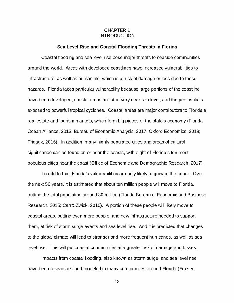
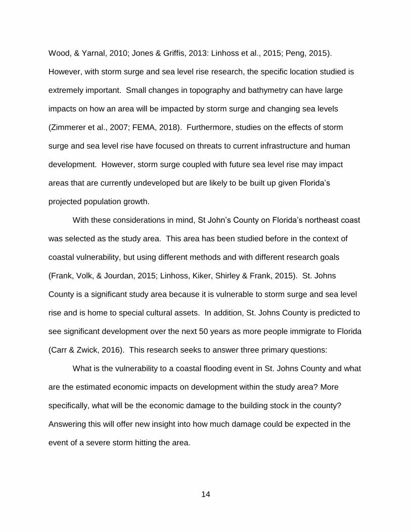
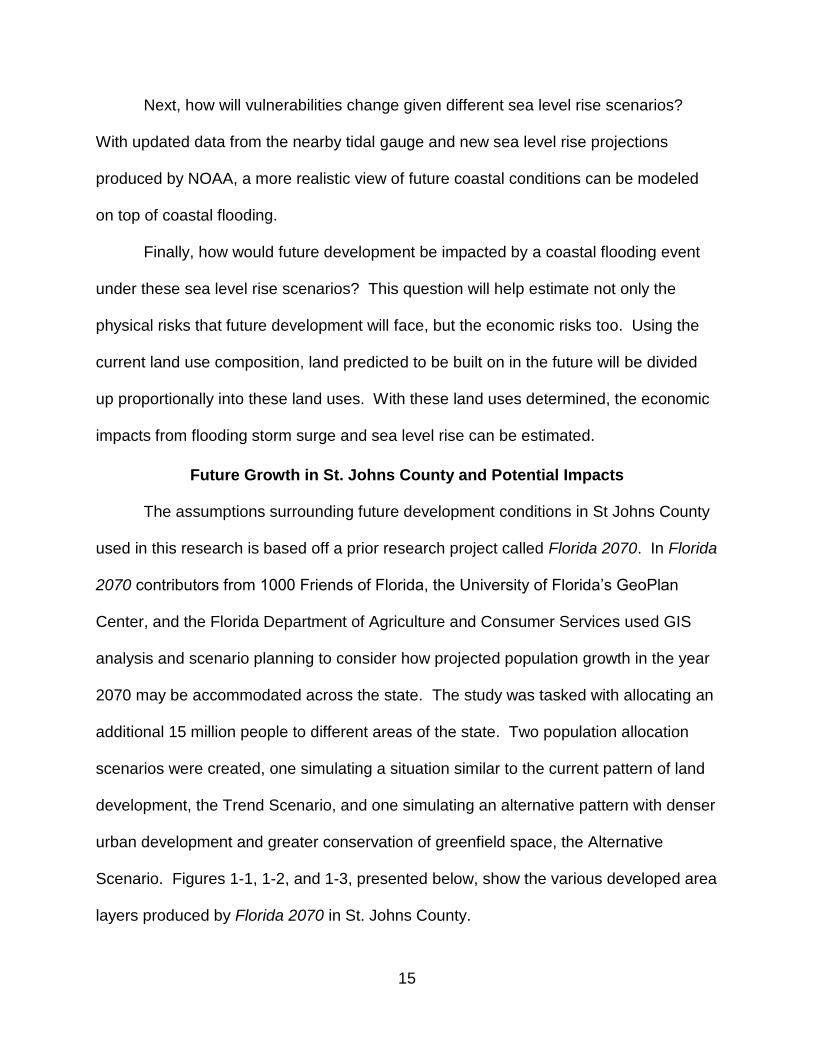
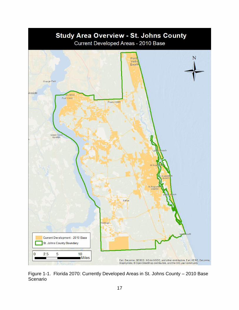
Future Growth in St. Johns County and Potential Impacts

The assumptions surrounding future development conditions in St Johns County

used in this research is based off a prior research project called Florida 2070. In Florida

2070 contributors from 1000 Friends of Florida, the University of Florida’s GeoPlan

Center, and the Florida Department of Agriculture and Consumer Services used GIS

analysis and scenario planning to consider how projected population growth in the year

2070 may be accommodated across the state. The study was tasked with allocating an

additional 15 million people to different areas of the state. Two population allocation

scenarios were created, one simulating a situation similar to the current pattern of land

development, the Trend Scenario, and one simulating an alternative pattern with denser

urban development and greater conservation of greenfield space, the Alternative

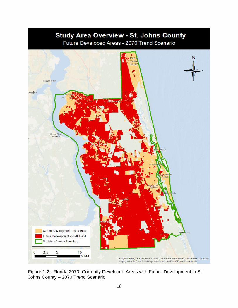
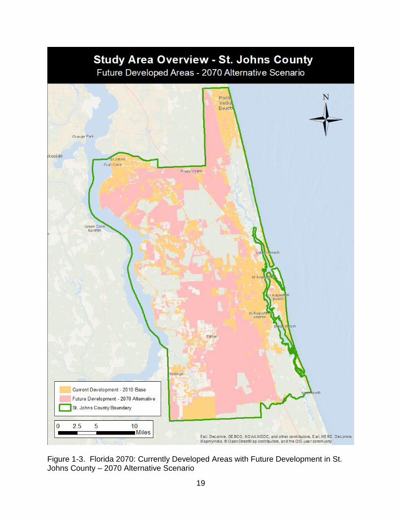
Scenario. Figures 1-1, 1-2, and 1-3, presented below, show the various developed area

layers produced by Florida 2070 in St. Johns County.

16

As mentioned previously, St. Johns County was selected as the study area

because of its current vulnerability to storm surge. However, it was also selected

because St. Johns is projected to see some of the largest population growth, by

percentage, of any county in the state. It is predicted that St. Johns will grow from a

2010 baseline of 190,039 to 591,272 in 2070, over a 3-fold increase (Carr & Zwick,

2016). Though some of the modeled development to accommodate population

increases in St. Johns will take place away from the coast, there are areas near the

coast which will be vulnerable. The robust results of the Florida 2070 study combined

with the coastal flooding and sea level rise models from Hazus enable novel research to

take place. Analyzing the impact of storm surge coupled with future sea level rise on

not only currently developed areas, but on areas likely to be developed in the future will

give a greater understanding of the potential impacts of storm surge and sea level rise

on the built environment in St. Johns County.

17

Figure 1-1. Florida 2070: Currently Developed Areas in St. Johns County – 2010 Base Scenario

18

Figure 1-2. Florida 2070: Currently Developed Areas with Future Development in St. Johns County – 2070 Trend Scenario

19

Figure 1-3. Florida 2070: Currently Developed Areas with Future Development in St. Johns County – 2070 Alternative Scenario

20

Research Outcomes

The outcomes of this research show that there is significant vulnerability to

coastal flooding events in St. Johns County. A 100-year storm with no additional sea

level rise could flood an estimated 40,000 acres of land and cause between $850 million

and $1.1 billion in damage to buildings. With just over two feet of sea level rise, a 100-

year storm could inundate nearly 50,000 acres of land. And with almost five and a half

feet of sea level rise, a 100-year storm could impact nearly 58,000 acres of land. These

impacts from flooding with sea level rise translate to between about $1.0 billion and $4.5

billion of damage to buildings in St. Johns County, depending on the flooding scenario.

Future development in St. Johns County is also expected to experience major

impacts from coastal flooding events. An additional 180,000 acres of land is projected

to be developed in St. Johns County. Of this total area, between 4,000 and 7,200 acres

are predicted to be inundated by 100-year coastal flooding events, depending on the

sea level rise scenario. Though this is a small amount compared to the total area of

future developed, the economic impacts would be significant. The estimated impact to

buildings in future development is between $1.6 and $4.9 billion in 2070 dollars.

Results will be discussed in greater detail in later chapters.

In chapter two, the foundation for the research conducted in this paper will be laid

out. The theoretical basis behind sea level rise forecasting, storm surge modeling, and

estimating impacts to the built environment will be discussed. Chapter three will

elaborate on the methodologies used in the study. This will cover data acquisition, data

management, the modeling workflow, and impact analysis workflow. Chapter four will

present results of the coastal flooding and sea level rise analysis. The modeled extent

21

of coastal flooding with and without sea level rise scenarios will be shown. Chapter five

will present the results of the economic impact analysis. Estimated impacts to current

and future development will be presented. Chapter six will provide a discussion and

conclusion. The results and their implications for St. Johns County will be discussed.

Conclusions regarding planning for future coastal flooding events and sea level rise,

along with research limitations will close the paper.

22

CHAPTER 2 LITERATURE REVIEW

The basis for this research is built on three broad areas of prior research: sea

level rise forecasting, modeling of coastal flooding, and estimating impacts of flooding

events.

Sea Level Rise Forecasting

A variety of documents and tools are available which offer forecasts of how future

sea level rise may impact the globe as well as more specific regions. The

Intergovernmental Panel on Climate Change (IPCC) is a well-known international

organization which has provided a variety of reports on climate change and its

outcomes. The most recent major document produced by the IPCC is the Fifth Annual

Report (AR5). In this document, among other climate change-related issues, the IPCC

describes various sea level rise concepts such as Global Mean Sea Level, Relative Sea

Level Rise, Regional Sea Level, and Local Sea Level. These different concepts

describe why the same amount of sea level rise is not seen everywhere and how in

some locations negative sea level rise may be observed. In addition to these concepts,

multiple sea level rise scenarios are discussed. When considering global mean sea

level rise, the IPCC predicts that between 2046 and 2065 sea levels rise will likely be

0.17 to 0.38 meters (0.56 to 1.25 feet) (IPCC, 2014). Between 2081 and 2100 the IPCC

predicts a global mean sea level rise of between 0.26 and 0.82 meters (0.85 to 2.69

feet) will be observed (IPCC, 2014). With these broad ranges of global sea level rise in

mind, other sources for regional or local sea level rise will be discussed.

The National Oceanic and Atmospheric Administration (NOAA) produce data and

reports describing sea level rise around the US. NOAA uses a network of tide gauge

23

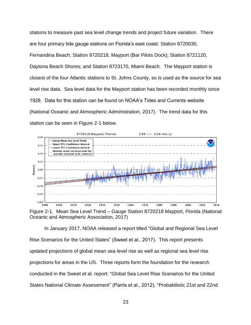
stations to measure past sea level change trends and project future variation. There

are four primary tide gauge stations on Florida’s east coast: Station 8720030,

Fernandina Beach; Station 8720218, Mayport (Bar Pilots Dock); Station 8721120,

Daytona Beach Shores; and Station 8723170, Miami Beach. The Mayport station is

closest of the four Atlantic stations to St. Johns County, so is used as the source for sea

level rise data. Sea level data for the Mayport station has been recorded monthly since

1928. Data for this station can be found on NOAA’s Tides and Currents website

(National Oceanic and Atmospheric Administration, 2017). The trend data for this

station can be seen in Figure 2-1 below.

Figure 2-1. Mean Sea Level Trend – Gauge Station 8720218 Mayport, Florida (National Oceanic and Atmospheric Association, 2017) In January 2017, NOAA released a report titled “Global and Regional Sea Level

Rise Scenarios for the United States” (Sweet et al., 2017). This report presents

updated projections of global mean sea level rise as well as regional sea level rise

projections for areas in the US. Three reports form the foundation for the research

conducted in the Sweet et al. report: “Global Sea Level Rise Scenarios for the United

States National Climate Assessment” (Parris et al., 2012), “Probabilistic 21st and 22nd

24

century sea-level projections at a global network of tide-gauge sites” (Kopp et al., 2014),

and “Regional Sea Level Scenarios for Coastal Risk Management: Managing the

Uncertainty of Future Sea Level Change and Extreme Water Levels for Department of

Defense Coastal Sites Worldwide” (Hall et al., 2016). The work of Parris et al. set a

precedent for sea level rise research in the US. It worked to coordinate sea level rise

scenario planning and resulted in creating four Global Mean Sea Level (GMSL) rise

scenarios to help planners and policy-makers consider various risk levels in the future

(2012).

However, the work Parris et al. focused on global mean sea levels. Research by

Kopp et al. (2014) and Hall et al. (2016) sought to generate more localized Regional

Sea Level (RSL) rise estimates, accounting for local variations such as land subsidence

and variability in ocean circulation. The researchers used the Parris et al. (2012) results

as a basis for their work. Kopp et al. generated probabilistic sea level projections at a

global network of tide gauge sites (2014). Hall et al. uses the scenarios from Parris et

al. (2012) as “a foundation for identifying local and regional sea level change scenarios”

(2016, pg. 2-9).

Sweet et al. use these two reports as the foundation for developing RSL rise

scenarios for the US. Particularly important in the report is the incorporation the most

up-to-date science and methodologies for adjusting GMSL rise scenarios to a specific

region (Sweet et al., 2017). The report produces six scenarios for 2100 based on

GMSL scenarios. The GMSL rise scenarios are: Low (0.3 meters), Intermediate-Low

(0.5 meters), Intermediate (1.0 meters), Intermediate-High (1.5 meters), High (2.0

meters), and Extreme (2.5 meters) (Sweet et al., 2017). In addition, GMSL scenarios

25

were calculated for each decade based on 19-year averages (Sweet et al., 2017).

These GMSL scenarios were used to calculate RSL scenarios and can be viewed using

a tide gauge station as a reference point. A simple way to view the RSL rise projections

at each station is by using the US Army Corps of Engineers (USACE) Sea Level Curve

Calculator. Using the online tool provided by the USACE, a user can select from

multiple sea level rise scenario sources. The NOAA 2017 report by Sweet et al. is

included as an option. Simply by selected the Mayport gauge station and the NOAA

2017 scenario source the user can view the different GMSL projections at the Mayport

location (USACE Sea Level Change Curve Calculator, 2017).

Modeling Coastal Flooding

Coastal flooding, commonly called storm surge, poses major risks for

communities in coastal areas. Many techniques have been developed to model the

extent and depth of flooding given a variety of parameters. Typically, these models are

produced by government bodies, like NOAA or FEMA, or by academic institutions.

Examples include SLOSH, ADCIRC, SWAN, WHAFIS, and RUNUP. The calculations

and computer programs used to run these models are complex. The required inputs for

these models varies based on the fluid mechanics and three-dimensional models they

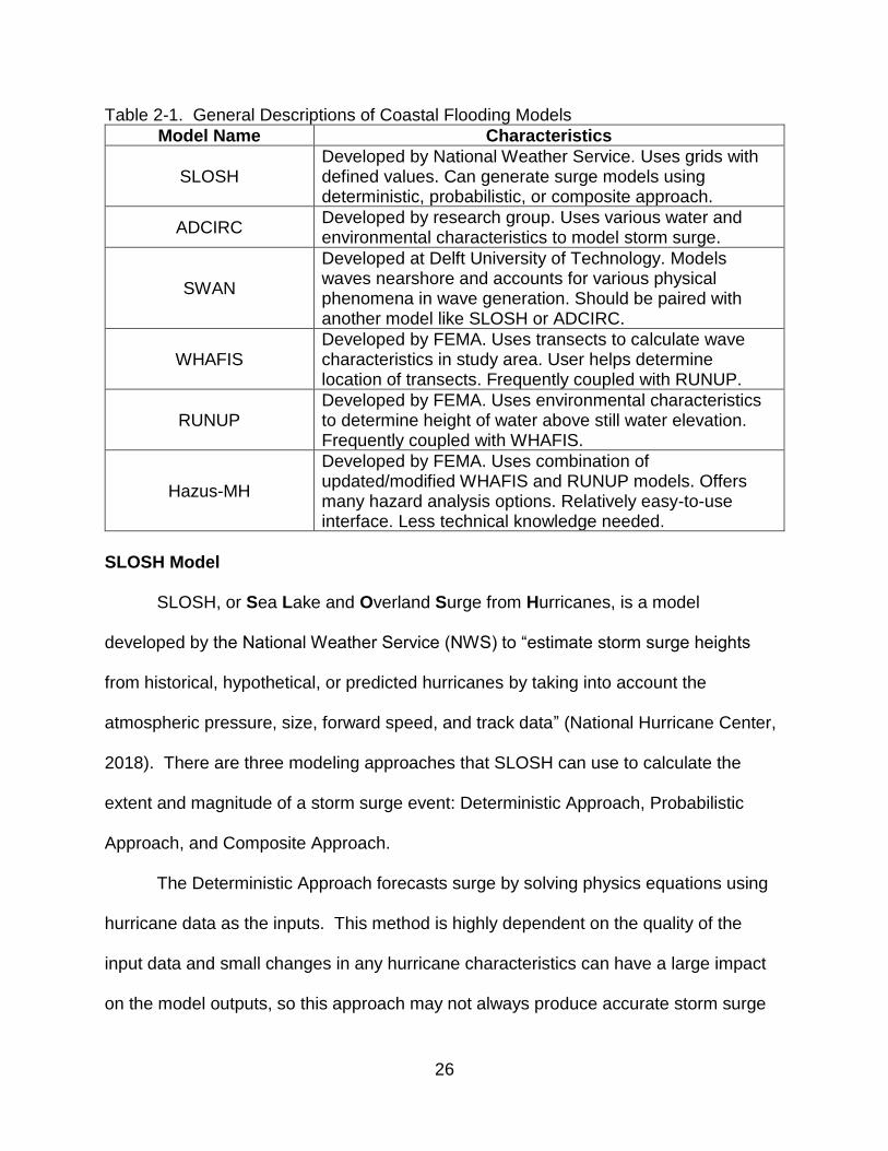
use. Table 2-1 below provides an overview of the models reviewed and then they are

described in greater detail.

26

Table 2-1. General Descriptions of Coastal Flooding Models

Model Name Characteristics

SLOSH Developed by National Weather Service. Uses grids with defined values. Can generate surge models using deterministic, probabilistic, or composite approach.

ADCIRC Developed by research group. Uses various water and environmental characteristics to model storm surge.

SWAN

Developed at Delft University of Technology. Models waves nearshore and accounts for various physical phenomena in wave generation. Should be paired with another model like SLOSH or ADCIRC.

WHAFIS Developed by FEMA. Uses transects to calculate wave characteristics in study area. User helps determine location of transects. Frequently coupled with RUNUP.

RUNUP Developed by FEMA. Uses environmental characteristics to determine height of water above still water elevation. Frequently coupled with WHAFIS.

Hazus-MH

Developed by FEMA. Uses combination of updated/modified WHAFIS and RUNUP models. Offers many hazard analysis options. Relatively easy-to-use interface. Less technical knowledge needed.

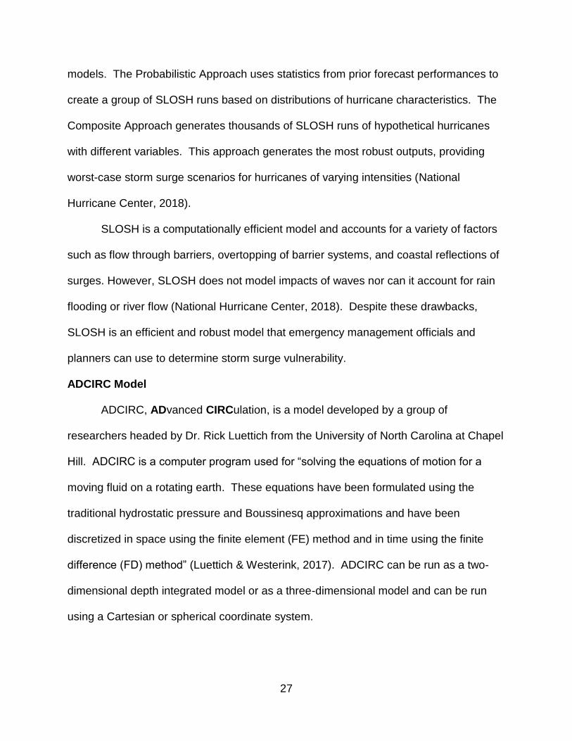
SLOSH Model

SLOSH, or Sea Lake and Overland Surge from Hurricanes, is a model

developed by the National Weather Service (NWS) to “estimate storm surge heights

from historical, hypothetical, or predicted hurricanes by taking into account the

atmospheric pressure, size, forward speed, and track data” (National Hurricane Center,

2018). There are three modeling approaches that SLOSH can use to calculate the

extent and magnitude of a storm surge event: Deterministic Approach, Probabilistic

Approach, and Composite Approach.

The Deterministic Approach forecasts surge by solving physics equations using

hurricane data as the inputs. This method is highly dependent on the quality of the

input data and small changes in any hurricane characteristics can have a large impact

on the model outputs, so this approach may not always produce accurate storm surge

27

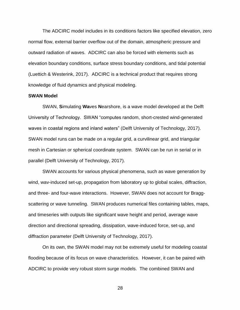
models. The Probabilistic Approach uses statistics from prior forecast performances to

create a group of SLOSH runs based on distributions of hurricane characteristics. The

Composite Approach generates thousands of SLOSH runs of hypothetical hurricanes

with different variables. This approach generates the most robust outputs, providing

worst-case storm surge scenarios for hurricanes of varying intensities (National

Hurricane Center, 2018).

SLOSH is a computationally efficient model and accounts for a variety of factors

such as flow through barriers, overtopping of barrier systems, and coastal reflections of

surges. However, SLOSH does not model impacts of waves nor can it account for rain

flooding or river flow (National Hurricane Center, 2018). Despite these drawbacks,

SLOSH is an efficient and robust model that emergency management officials and

planners can use to determine storm surge vulnerability.

ADCIRC Model

ADCIRC, ADvanced CIRCulation, is a model developed by a group of

researchers headed by Dr. Rick Luettich from the University of North Carolina at Chapel

Hill. ADCIRC is a computer program used for “solving the equations of motion for a

moving fluid on a rotating earth. These equations have been formulated using the

traditional hydrostatic pressure and Boussinesq approximations and have been

discretized in space using the finite element (FE) method and in time using the finite

difference (FD) method” (Luettich & Westerink, 2017). ADCIRC can be run as a two-

dimensional depth integrated model or as a three-dimensional model and can be run

using a Cartesian or spherical coordinate system.

28

The ADCIRC model includes in its conditions factors like specified elevation, zero

normal flow, external barrier overflow out of the domain, atmospheric pressure and

outward radiation of waves. ADCIRC can also be forced with elements such as

elevation boundary conditions, surface stress boundary conditions, and tidal potential

(Luettich & Westerink, 2017). ADCIRC is a technical product that requires strong

knowledge of fluid dynamics and physical modeling.

SWAN Model

SWAN, Simulating Waves Nearshore, is a wave model developed at the Delft

University of Technology. SWAN “computes random, short-crested wind-generated

waves in coastal regions and inland waters” (Delft University of Technology, 2017).

SWAN model runs can be made on a regular grid, a curvilinear grid, and triangular

mesh in Cartesian or spherical coordinate system. SWAN can be run in serial or in

parallel (Delft University of Technology, 2017).

SWAN accounts for various physical phenomena, such as wave generation by

wind, wav-induced set-up, propagation from laboratory up to global scales, diffraction,

and three- and four-wave interactions. However, SWAN does not account for Bragg-

scattering or wave tunneling. SWAN produces numerical files containing tables, maps,

and timeseries with outputs like significant wave height and period, average wave

direction and directional spreading, dissipation, wave-induced force, set-up, and

diffraction parameter (Delft University of Technology, 2017).

On its own, the SWAN model may not be extremely useful for modeling coastal

flooding because of its focus on wave characteristics. However, it can be paired with

ADCIRC to provide very robust storm surge models. The combined SWAN and

29

ADCIRC models have been used in a variety of research efforts (Chen et al., 2013;

Jones and Griffis, 2013; Sebastian et al., 2014; Xie, Zou & Cannon, 2016).

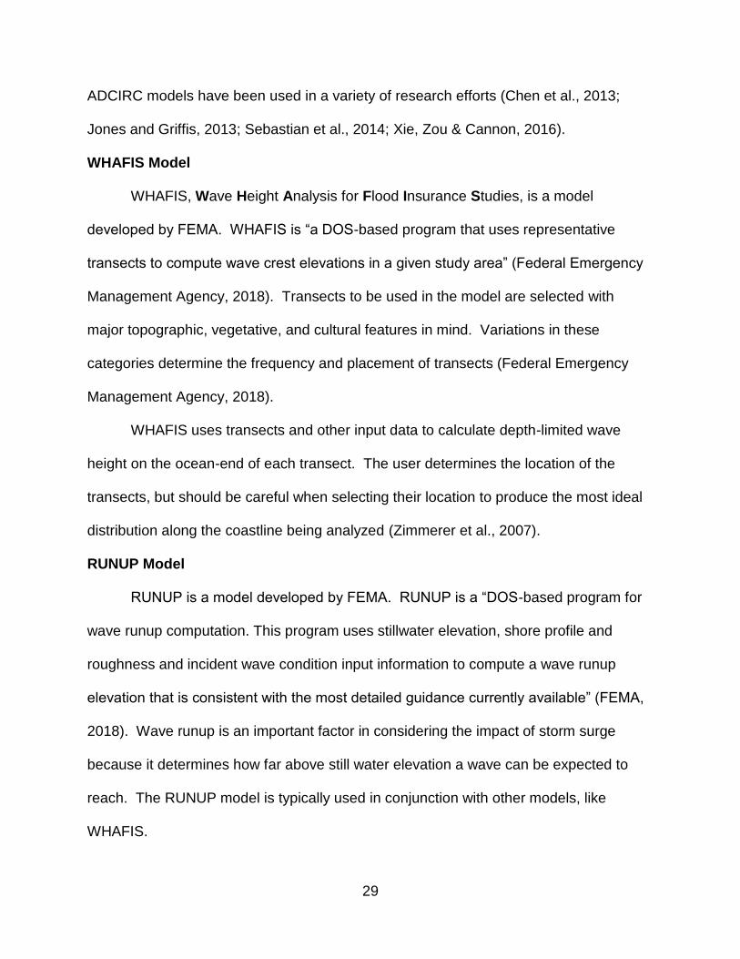
WHAFIS Model

WHAFIS, Wave Height Analysis for Flood Insurance Studies, is a model

developed by FEMA. WHAFIS is “a DOS-based program that uses representative

transects to compute wave crest elevations in a given study area” (Federal Emergency

Management Agency, 2018). Transects to be used in the model are selected with

major topographic, vegetative, and cultural features in mind. Variations in these

categories determine the frequency and placement of transects (Federal Emergency

Management Agency, 2018).

WHAFIS uses transects and other input data to calculate depth-limited wave

height on the ocean-end of each transect. The user determines the location of the

transects, but should be careful when selecting their location to produce the most ideal

distribution along the coastline being analyzed (Zimmerer et al., 2007).

RUNUP Model

RUNUP is a model developed by FEMA. RUNUP is a “DOS-based program for

wave runup computation. This program uses stillwater elevation, shore profile and

roughness and incident wave condition input information to compute a wave runup

elevation that is consistent with the most detailed guidance currently available” (FEMA,

2018). Wave runup is an important factor in considering the impact of storm surge

because it determines how far above still water elevation a wave can be expected to

reach. The RUNUP model is typically used in conjunction with other models, like

WHAFIS.

30

Hazus-MH

The storm surge models listed above are fairly complex. They can require

understanding of complex fluid dynamic models, with many required inputs to

successfully run the program. This can make using these tools too cumbersome for

planners and other stakeholders who don’t have a knowledge of fluid dynamics and

complex physics. To offer another option, FEMA created the Hazus-MH tool, a program

connected to the ArcGIS framework. Hazus allows users to view impacts from a variety

of natural hazards, including coastal flooding events. Hazus utilizes a nationally

applicable standard methodology, offering flexible options for generating outputs

(FEMA, 2018).

The coastal flooding modeling functionality in Hazus uses a general approach

and methodology similar to those that FEMA uses to generate coastal Flood Insurance

Rate Maps. These methods include drawing transects perpendicular to shorelines;

calculating water surface elevations, flood depths, and flood hazard zones; and

determining which models to run along each transect based on shoreline characteristics

and wave conditions (Department of Homeland Security, 2013).

This may sound similar to the WHAFIS and RUNUP models. In fact, these

models are used within Hazus to generate flood boundaries. However, it is noted in

documentation that these models included in the Hazus tool contain simplifications

compared to the full-blown WHAFIS and RUNUP models. These simplifications enable

users to model storm surge events with less input and knowledge than required in the

standard models. It is also noted in the documentation, though, that the models used in

31

the Hazus tool include improvements made to some aspects of the models by including

more recent scientific developments (Department of Homeland Security, 2013).

Estimating Impacts of Coastal Flooding Events

There is extensive literature focused on estimating the economic impacts of

coastal flooding and sea level rise on the built environment. This research can be

broken down into two varieties, one group considering only the direct impacts of a

hazard on property and the other group considering additional indirect costs such as

lost income, relocation costs, and price changes. Additionally, these studies typically

consider only the impacts of storm surge or sea level rise (Yohe et al., 1996; Tol, 2002;

Stanton, Davis, & Fencl, 2010; Linhoss et al., 2015). However, more and more

researchers have recognized that future sea level rise will only make coastal flooding

events more damaging by raising the base sea level (Kleinosky, Yarnal, & Fisher, 2006;

Frazier, Wood, & Yarnal, 2010; Peng, 2015; Withey, Lantz, & Ochuodho, 2015).

Genovese and Green analyze how flood depth, using outputs from the SLOSH

model, in South Florida may impact buildings, both property and contents, in the

absence and presence of coastal protection (2014). Using flood depth, flood extent,

damage functions for different building classifications, and land use information for

properties they are able to estimate the economic impacts when SLOSH outputs

overlap with properties (Genovese & Green, 2014).

Hazus-MH Impact Analysis

After determining flood depth and extent in Hazus, described in the section

above, the software offers built-in flood loss estimation analysis. Hazus can implement

two different methodologies specific to building damage, a full replacement cost or a

32

depreciated cost model (Department of Homeland Security, 2013). The methodology

for the full replacement cost is more significant as it relates to this research, so will be

the focus of this review.

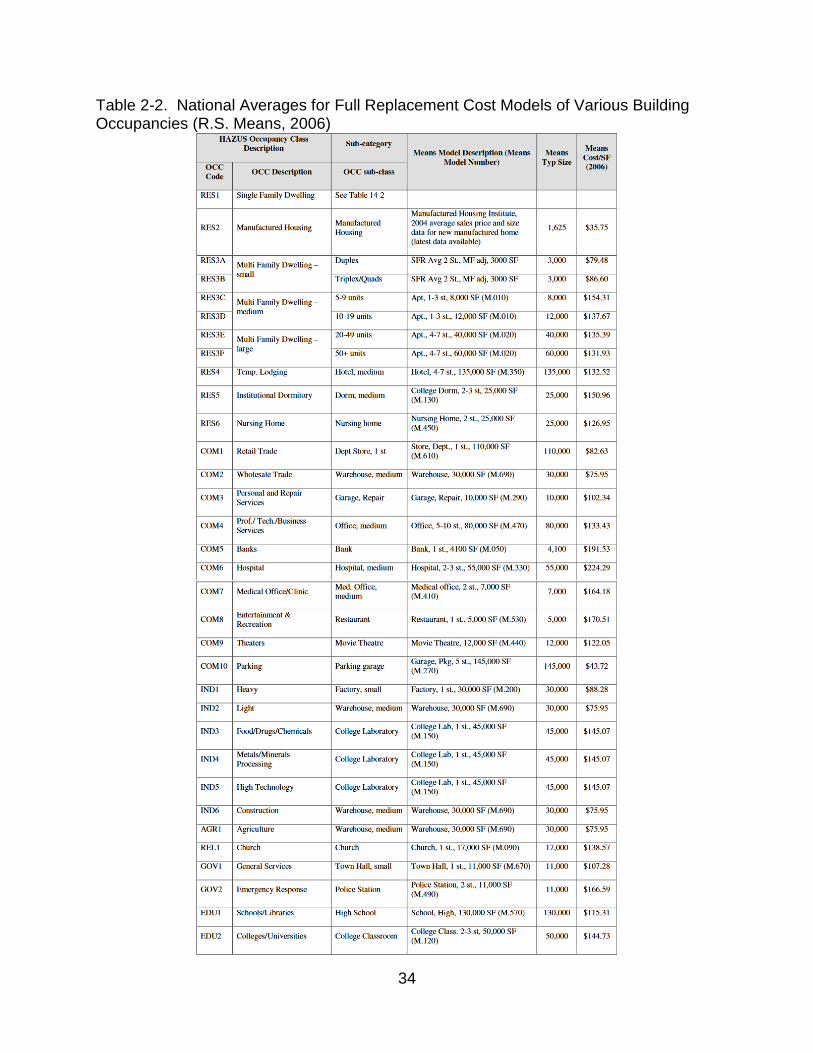
Building replacement cost models in Hazus are built on industry-standard models

available in the 2006 Means Square Foot Costs by R.S. Means. Replacement cost data

is stored at the census block level for each type of building occupancy. The census

block represents the highest level of economic impact analysis within the Hazus

framework. A default structure replacement cost, using cost for square foot as the

measurement unit, is provided in the software for each occupancy class. These

replacement costs can be viewed in Table 2-2 below. Square foot costs shown in the

table were averaged for various building materials (Department of Homeland Security,

2013).

Of the occupancy classes, the single family residential replacement cost model is

the most intricate. It uses socio-economic data from each census block to help provide

a more accurate mix of replacement cost models. The algorithm used to determine total

estimated valuation for single family residences includes the following factors: total area

in square feet of single family residences in a census block, the Means construction

class, the weighting factor for the construction class, the number of stories, the

weighting factor for number of stories, the cost per square foot of single family

residential given the construction class and number of stories, the presence of a

basement, the weighting factor for basement presence, the additional cost per square

foot for a finished basement given the construction class and number of stories, the

weighting factor for garage type, additional replacement cost for garage type, and count

33

of single family residential structures within a census block (Department of Homeland

Security, 2013).

The remaining algorithms used to estimate replacement cost for the different

occupancy classes are far less complex. First, a specific algorithm for replacement cost

of manufactured housing, more specifically mobile homes, is used. The factors used to

determine total valuation for manufactured housing includes: total floor area in square

feet of manufactured housing and the cost per square foot. The other algorithm used

includes all other residential building types and all non-residential building types. This

algorithm incorporates potential for number of stories. The factors used to determine

the other building valuations include: total floor area in square feet for a specific building

type in a census block and the cost per square foot of the building occupancy type

(Department of Homeland Security, 2013).

34

Table 2-2. National Averages for Full Replacement Cost Models of Various Building Occupancies (R.S. Means, 2006)

35

Hazus Impact Analysis Comparison

The Hazus methodology is robust and includes region-specific information based

on the location of the study area. However, with the highest resolution of data being at

the census block scale, some even higher level local variations can be smoothed over

in the analysis. Karamouz et al. utilize an alternative method to the Hazus impact

analysis methodology (2016). In the study they compare Hazus outputs with their

alternative methods. They use four general inputs to model impacts: the floodplain, the

DEM, land-use data, and depth-damage functions. They use zonal statistics to assign

the maximum water level to each polygon of land use, classified into three major

categories: residential, industrial, and commercial. After gathering this necessary

information by land use category, depth damage curves were applied based on land

use to determine the economic impact of flooding (Karamouz et al., 2016).

Karamouz et al. conducted a case study on the island of Manhattan in New York

City, NY (2016). They ran the Hazus impact analysis methodology then their own

methodology to compare estimations of impacts to buildings. Overall, their models

estimated lower economic loss estimates for structural impacts compared to the Hazus

predictions when using Flood Insurance Study information. In their conclusions, they

discuss how the incorporation of higher resolution tax-parcel data into the land use and

damage modeling can lead to more accurate estimations of building impacts from

flooding (Karamouz et al., 2016).

36

CHAPTER 3 METHODOLOGY

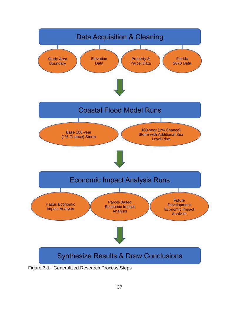
The goal of this research is to produce a clear and systematic analysis of storm

surge impacts on property to consider how current and future development will need to

act to minimize and, if possible, avoid losses from natural hazards. By laying out a

repeatable methodology, others may use these methods to estimate impacts in other

communities. A flow chart of the research process steps can be seen in Figure 3-1

below.

An online US Army Corps of Engineers resource was used to estimate future sea

level rise and a FEMA Flood Insurance Study (FIS) was used to determine expected

sea levels during a storm event in the study area. The Hazus-MH tool was selected to

model coastal flooding. Hazus was selected because of its relative ease-of-use, its

intuitive connection within ArcGIS architecture, the relative simplicity of required inputs,

and the useful. ArcGIS software was used further to conduct impact analysis on

developed areas and understand how future development may be impacted by storm

surge and sea level rise.

37

Figure 3-1. Generalized Research Process Steps

Data Acquisition & Cleaning

Coastal Flood Model Runs

Study Area Boundary

Elevation Data

Property & Parcel Data

Florida 2070 Data

Base 100-year (1% Chance) Storm

100-year (1% Chance) Storm with Additional Sea

Level Rise

Economic Impact Analysis Runs

Hazus Economic Impact Analysis

Parcel-Based Economic Impact

Analysis

Synthesize Results & Draw Conclusions

Future Development

Economic Impact Analysis

38

Data Acquisition

There are four broad groups of data that are necessary to complete this

research. They are: inputs into the Hazus-MH model, Hazus-MH outputs, parcel data

from St. Johns County, and Florida 2070 development projection data.

Hazus-MH Inputs

There are three major inputs into the Hazus-MH model. Hazus requires the user

to provide the study region which outlines the area of interest, a Digital Elevation Model

(DEM) which details elevations across the study region, and specific parameters for a

coastal flooding scenario. With these inputs, the user can successfully run a coastal

flooding analysis. Some of the data is provided out-of-the-box in the Hazus software or

can be acquired through the prescribed workflow. However, the user can provide their

own data for some inputs and must provide their own inputs for the scenario

parameters.

The study region is selected within the Hazus model. The user can choose

based on a spatial hierarchy from census block level up to an entire state. St. Johns

county was selected as the study area. A custom DEM was used. The DEM was a

mosaic of two DEMs, one created by the UF GeoPlan Center called FLIDAR and the

other from the United States Geological Service National Elevation Dataset. The two

DEMs were processed to ensure they covered St. Johns county, then pieced together

using the Raster Calculator tool in ArcToolbox. The specific calculation can be found in

the workflow described in Appendix A. Finally, scenario parameters were derived from

FEMA FIS reports. These reports are created for each county and updated periodically.

The FIS report describes 100-year flood still water elevation levels (SWEL) for different

39

coastal transects throughout the county. Using these values, the user can generate a

single 100-year SWEL to be used for the entire coastline in the model or the study

region coastline can be split up into multiple sections with different SWEL values. With

these values, the user can then add on any additional potential sea level rise as

desired. The result is a number of different SWELs, each representing a certain coastal

flooding scenario. The user must also determine the spatial datum, in this case

NAVD88, which defines certain elevation reference points in the model. With these

inputs in hand the Hazus coastal flooding model can be run.

The parameters used in the various coastal flooding scenarios are determined

from Flood Insurances Studies (FIS) produced by FEMA. These studies are conducted

for each county and are updated periodically. Currently there is an updated FIS for St.

Johns County that is under review, meaning that FEMA produced a final report, but may

need to make some minor edits before releasing the finalized version. The report was

released on May 16th, 2016. Despite the preliminary nature of the report, it was used in

this study to help provide still water elevations (SWELs) for the study area because it

supplied the most up-to-date information and is likely a good representation of

conditions in St. Johns County. The 100-year SWELs were derived from the FIS report

and used later the coastal flooding analysis.

It is essential to recognize that the study area selected only models coastal

flooding on the eastern side of St. Johns county. Though in reality flooding impacts may

be observed on the western side of the county from the St. Johns River, these are not

included in the model outputs. If the inclusion of this potential flooding source is

desired, the study region would need to be expanded to so that hydro-connectivity

40

between the Atlantic Ocean and the St. Johns River is explicitly present. As the study

region is, the river is isolated from the ocean so only oceanside coastal flooding is

modeled.

Hazus-MH Outputs

There are two important outputs that the Hazus-MH model generates which are

used in further analysis in the research. These are flood depth grids and impact

analysis outputs. Flood depth grids come in the form of raster grids and are produced

for the entire study area. Each cell in the grid contains a specific flood water depth and

the size of the cell is determined by the resolution of the DEM input by the user. The

flood depth grids are then used within the Hazus software as well as in analyses outside

of Hazus. Maps showing the extent and depth of the flood depth grids for each flooding

scenario can be seen in Appendix C.

The impact analysis outputs describe economic impacts to infrastructure such as

buildings, essential facilities, and the transportation network. These outputs can be

visualized in polygon layers within the ArcGIS framework or can be output into PDF

tables. These values are used later to compare economic impacts of various flooding

scenarios. Further description of these economic impact outputs can be seen in the

“Current Development Economic Impact Analysis” section below.

St. Johns County Parcel Data

St. Johns County parcel data is downloaded from the St. Johns County Property

Appraiser. The property appraiser maintains the most up-to-date parcel and property

datasets for the county. This data is used is used in the “Custom Level 2” impact

analysis, which will be described later. Having the most up-to-date property information

41

ensures that the impact analysis is as accurate as possible. These datasets were

downloaded from the St. Johns County Property Appraiser website

(https://www.sjcpa.us/formsdata/).

The files were downloaded on December 20, 2017 and came in the form of

zipped file folders. The files downloaded were: GIS Data Bundle, CAMA Data Bundle,

and CAMA Data Supplemental Bundle. The data in the GIS Data Bundle came in the

form of a file geodatabase, while the two CAMA Bundles came in Microsoft Access

databases and excel spreadsheets. The key feature class from the GIS Data Bundle,

within the file geodatabase, was the Parcel feature class. The key tables within the

Access databases were the ParcelView table, from the CAMA Data Bundle, and the

BldView and the StructElemViewUnit tables, from the CAMA Data Supplemental

Bundle.

The Access tables were exported to excel spreadsheets within Access and then

converted from excel files to file geodatabase tables using the Excel to Table tool in

ArcMap. This method was used because it preserved a key piece of information, the

Parcel ID Number, most effectively. This ensured that linking attribute information

between the parcel feature class and other tables through joins would be successful.

Florida 2070 Development Projection Data

In the Florida 2070 study, population growth projections were taken from the

Florida Bureau of Economic and Business Research (BEBR) and a statewide

population of 33.7 million residents in 2070 was used. The baseline population

condition used in the study is from the 2010 census, where a total population of

42

18,801,310 was counted. An increase of nearly 15 million people over 60 years serves

as a defining value for the study (Carr & Zwick, 2016).

Development densities for the Trend and Alternative scenarios were determined

on a county by county basis and these densities were used to allocate population based

on various land use categories. In the Trend Scenario, no new population was added to

allocated to existing developed areas and was allocated to new development using

suitability surfaces and the gross development density for each county. In the

Alternative Scenario, some of the new population was added to existing urban areas

with the remaining population added using similar suitability layers but with an increased

development density. These differences in population allocation show how more

undeveloped lands can be kept in their current state, protecting important agricultural

resources and natural habitats. It also can help prevent development from straying into

areas that may be vulnerable to future impacts of storm surge and sea level rise (Carr &

Zwick, 2016).

The Florida 2070 project produced a variety of outputs. These include reports

outlining data inputs, methodology, and results. These documents provide stakeholders

and other researchers insight into the project, showing how the methods may be

replicated to generate the outputs described or may be tweaked to fit other locations.

However, the key datasets for this thesis research are spatial datasets describing the

extent of development in Florida. Two polygon layers are particularly important: one

detailing the developed land area in 2010 and one predicting the developed land area in

2070 if current trend land development practices continue. These datasets will be used

43

to consider how predicted future development in St. Johns County may be impacted by

different coastal flooding scenarios.

Though Florida 2070 also produced the Alternative Scenario, this was left out of

the analysis. This decision was made because assumptions regarding future

development densities were more difficult to accurately replicate in the economic impact

analysis. Only including the Trend development scenario in the future economic impact

analysis minimizes assumptions that must be made when processing the data. The

breakdown of land use types for the future developed areas in the Trend scenario can

be derived from parcel information from St. Johns County Property Appraiser,

mentioned above.

The 2010 Base and 2070 Trend spatial datasets were downloaded from the

Florida Geographic Data Library, FGDL (https://fgdl.org/metadataexplorer/explorer.jsp).

Maps showing these datasets can be seen in Chapter 1, displayed in Figures 1-1 & 1-2.

Hazus-MH Model Descriptions

The Hazus-MH model is developed by FEMA. According to FEMA, “Hazus is a

nationally applicable standardized methodology that contains models for estimating

potential losses from earthquakes, floods, and hurricanes. Hazus uses Geographic

Information Systems (GIS) technology to estimate physical, economic, and social

impacts of disasters” (FEMA, 2018). Hazus is a very useful tool because of the

standardized and straightforward methodology for modeling impacts.

This research utilizes flooding analysis within Hazus and more specifically, the

coastal flooding methodology. The coastal flooding model enables the user to simulate

anywhere from a 10% annual chance to a 0.2% annual chance, or a 10-year to a 500-

44

year, storm event. For this study, a 1% annual chance, or 100-year storm event, was

used. The input data needed to run the coastal flooding model is described in the

“Hazus-MH Inputs” section above, however it is important to note the data that the user

must input to successfully run the Hazus model is relatively light compared to other

coastal flooding models. The models that Hazus uses in coastal flooding analyses are

simplifications of the erosion, Wave Height Analysis for Flood Insurance Studies

(WHAFIS), and RUNUP models (Department of Homeland Security, 2013).

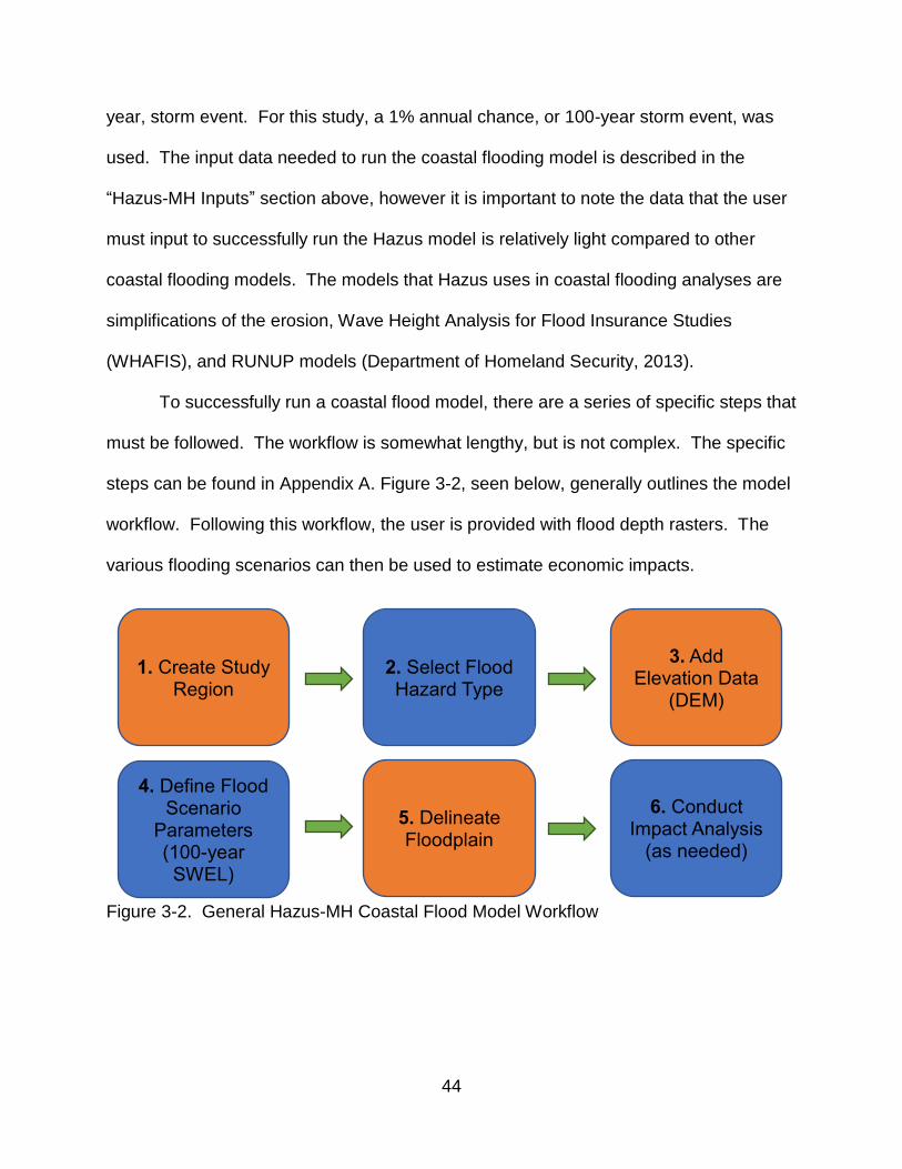
To successfully run a coastal flood model, there are a series of specific steps that

must be followed. The workflow is somewhat lengthy, but is not complex. The specific

steps can be found in Appendix A. Figure 3-2, seen below, generally outlines the model

workflow. Following this workflow, the user is provided with flood depth rasters. The

various flooding scenarios can then be used to estimate economic impacts.

Figure 3-2. General Hazus-MH Coastal Flood Model Workflow

1. Create Study Region

2. Select Flood Hazard Type

3. Add Elevation Data

(DEM)

4. Define Flood Scenario

Parameters (100-year SWEL)

5. Delineate Floodplain

6. Conduct Impact Analysis

(as needed)

45

Current Development Economic Impact Analysis

Estimating the economic impact of coastal flooding events, with and without

increases in sea level, is a key goal of this research. Listing the flood depths for and

showing the extent of flooding in the study area gives readers a visual and physical

understanding of impacts. However, it can be difficult to gauge how those values

translate to damage to infrastructure that people value, like homes and businesses. A

simple way to gauge economic impacts is to consider the impact of flooding on

buildings. Buildings have an inherent value that is not necessarily related to the location

of the building, but is tied to the type of building, age, size, and materials used. This

makes considering impacts on buildings an efficient proxy for measuring economic

impact. In the analysis, only impacts to buildings are considered. Other infrastructure,

such as transportation and utilities network, is not included. The Hazus software has

this capability built-in to the software. These have been described in the literature

review.

An issue noted with Hazus is that economic impacts to buildings are aggregated

at the census block level. In doing this, some of the granularity of the flooding analysis

is lost. This is because aggregating parcels to a census bock generalizes impacts and

building valuations are spread evenly across census blocks. As a result, it is possible

that Hazus overestimates economic impacts from flooding events because buildings are

frequently built on higher elevation portions of parcels. This means that buildings may

not actually be impacted by a flooding event even though Hazus counts it. In addition,

the specific valuations of infrastructure are generalized, so an expensive building that

may not be impacted will have its value averaged out across the census block.

46

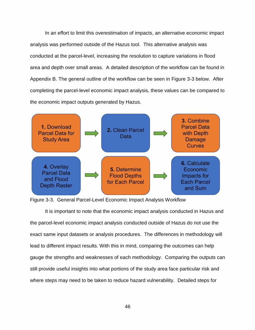
In an effort to limit this overestimation of impacts, an alternative economic impact

analysis was performed outside of the Hazus tool. This alternative analysis was

conducted at the parcel-level, increasing the resolution to capture variations in flood

area and depth over small areas. A detailed description of the workflow can be found in

Appendix B. The general outline of the workflow can be seen in Figure 3-3 below. After

completing the parcel-level economic impact analysis, these values can be compared to

the economic impact outputs generated by Hazus.

Figure 3-3. General Parcel-Level Economic Impact Analysis Workflow It is important to note that the economic impact analysis conducted in Hazus and

the parcel-level economic impact analysis conducted outside of Hazus do not use the

exact same input datasets or analysis procedures. The differences in methodology will

lead to different impact results. With this in mind, comparing the outcomes can help

gauge the strengths and weaknesses of each methodology. Comparing the outputs can

still provide useful insights into what portions of the study area face particular risk and

where steps may need to be taken to reduce hazard vulnerability. Detailed steps for

1. Download Parcel Data for

Study Area

2. Clean Parcel Data

3. Combine Parcel Data with Depth Damage Curves

4. Overlay Parcel Data and Flood

Depth Raster

5. Determine Flood Depths

for Each Parcel

6. Calculate Economic Impacts for Each Parcel

and Sum

47

completing the current development economic impact analysis can be found in

Appendix B.

Future Development Economic Impact Analysis

Measuring impact of coastal flooding and sea level rise on current development

is a crucial first step in understanding an area’s vulnerability and taking steps to improve

resiliency moving forward. However, the ability to estimate the amount of impact on

developed areas in the future is more difficult because it is hard to say where and how

development will take place. The Florida 2070 report offers us this glimpse into the

future, using sound assumptions and analysis methods to determine what areas will

likely be built up in the future. Using the area outlined which is projected to be

developed in 2070, we can estimate economic impact from coastal flooding events with

various additional amounts of sea level rise added onto a 1% annual chance coastal

flooding event.

The future development economic impact analysis is similar to the current

development economic impact analysis, with the addition of two other steps. After

combining parcel data with depth damage curves, the area to be considered for future

development must be determined. This is done by using the 2070 Trend developed

lands layer dataset from the Florida 2070 study. This dataset was acquired from FGDL.

The development boundaries in this layer includes the developed area from the base

scenario. These areas were removed from the data layers so that only lands projected

to be developed were considered. In addition, the parcels used in the current economic

impact analysis were used to erase areas developed after 2010 from the 2070 Trend

layer.

48

After isolating the future development area, the land use breakdown of the future

developed areas had to be established. For the Trend scenario, the same composition

of land uses seen in the parcel data was applied to the future development lands. The

land use breakdown was determined from specific occupancy, or generalized land use,

descriptions tied to specific depth damage curves. Based on the specific occupancy

information, average valuations of the land could also be determined. Hazus draws

from a database where this information is stored, and it can be used, along with inflation

rates, to determine the value of future developed lands.

It should be recognized that the 2070 Trend development scenario permits land

to be developed in areas that may be vulnerable to coastal flooding and sea level rise.

There are not necessarily any limitations to development, such as not permitting

building in floodplains. The qualifications for land that is considered for future

development can be found in the Florida 2070 project documentation.

By adding in these steps, future developed areas could then be overlaid with the

storm surge scenarios and the economic impact analysis process can be carried

through. Detailed steps for the future development economic impact analysis can be

found in Appendix B.

49

CHAPTER 4 COASTAL FLOODING AND SEA LEVEL RISE RESULTS

Hazus Coastal Flooding and Sea Level Rise Outputs

The first major set of outputs generated from the analysis are flood depth grids.

These grids, generated by the Hazus coastal flooding analysis, represent flood depth

and extent for the study area. To make the flood depth grids more visually intuitive, the

raster layers were clipped to land areas using a land cover dataset from FGDL. Table

4-1 below summarizes some basic flood depth grid statistics for the various scenarios

that were modeled. St. Johns County boundary was used as the area of consideration

for calculating flood statistics.

Table 4-1. Flood Statistics for Coastal Flooding Scenarios Incorporating Varying Amounts of Sea Level Rise in St. Johns County

Flooding Scenario Feet

of SLR Minimum

Flood Depth Maximum

Flood Depth Average

Flood Depth Flood Area

Base 0 0 ft 18.07 ft 4.42 ft 40826 ac

2070VLM 0.13 0 ft 18.19 ft 4.54 ft 41669 ac

2070Low 0.98 0 ft 19.05 ft 5.11 ft 44576 ac

2070IntermediateLow 1.25 0 ft 19.32 ft 5.24 ft 46776 ac

2070Intermediate 2.23 0 ft 20.29 ft 6.02 ft 49617 ac

2070IntermediateHigh 3.31 0 ft 21.38 ft 6.77 ft 52320 ac

2070High 4.49 0 ft 23.79 ft 7.68 ft 55265 ac

2070Extreme 5.41 0 ft 24.79 ft 8.32 ft 57760 ac

Increases in sea level rise have a noticeable impact on variations in maximum

flood depth, average flood depth, and area flooded. With additional amounts of sea

level rise added on, it can be seen how the maximum flood depths increase. The

maximum flood depth estimated in the study area ranges from just over 18 feet at the

base sea level scenario to nearly 25 feet at the most extreme scenario. It is important

to recognize that this increase is not linear, meaning that the maximum flood depth does

not increase by the same amount of sea level rise. For example, in the VLM scenario

0.13 feet of sea level is added but the maximum flood depth increases by only 0.12 feet.

50

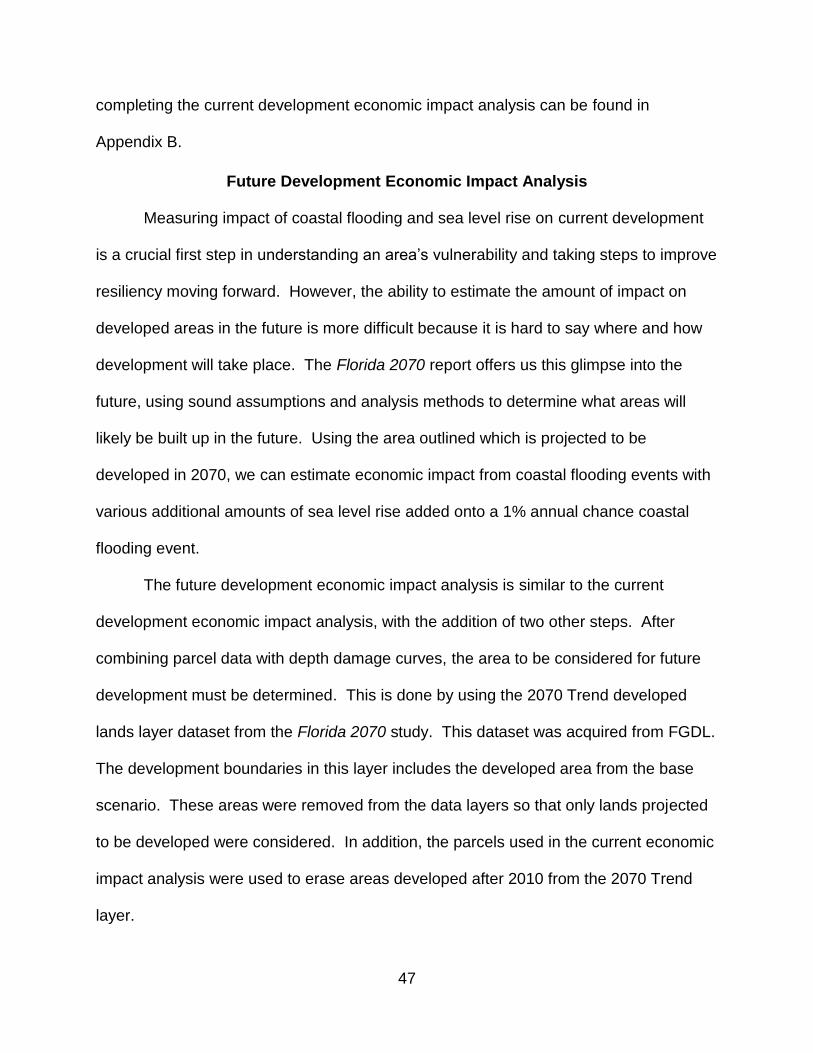
On the other hand, in the extreme scenario 5.41 feet of sea level is added and the

maximum flood depth increases by 6.72 feet. Average flood depth is also important to

consider. With nearly 5.5 feet of sea level rise over the base, average flood depth for

the study area nearly doubles.

This increase in flooding is noticeable especially when looking at the outputs

visually. In Figures 4-1, 4-2, and 4-3 below, a portion of the study area, near the city of

St. Augustine, is zoomed in to. Other maps of the flooding outputs can be seen in

Appendix C.

51

Figure 4-1. Hazus Coastal Flooding Output – Base Flooding Scenario in the St. Augustine Area

52

Figure 4-2. Hazus Coastal Flooding Output – 2070 Low Flooding Scenario in the St. Augustine Area

53

Figure 4-3. Hazus Coastal Flooding Output – 2070 High Flooding Scenario in the St. Augustine Area

54

CHAPTER 5 ECONOMIC IMPACT RESULTS

Economic impacts were estimated for current and future conditions in the study

area. Results are presented below.

Current Development Impact Results

Current Economic impacts for the study were using the Hazus program and

using a parcel-level analysis. First, the Hazus results will be presented, then the parcel-

level impacts will be presented.

Hazus Economic Impact Outputs

Hazus offers a variety of metrics describing economic impacts. These range

from analyzing impacts to critical facilities, to transportation networks, to vehicles. In

this research, economic impacts to buildings, excluding impacts to contents, were the

focus. As described in the methodology, a variety of land use types were used to help

determine how a range of flood depths would impact different building types. The

Hazus software calculates the impacts within the software, with the user simply

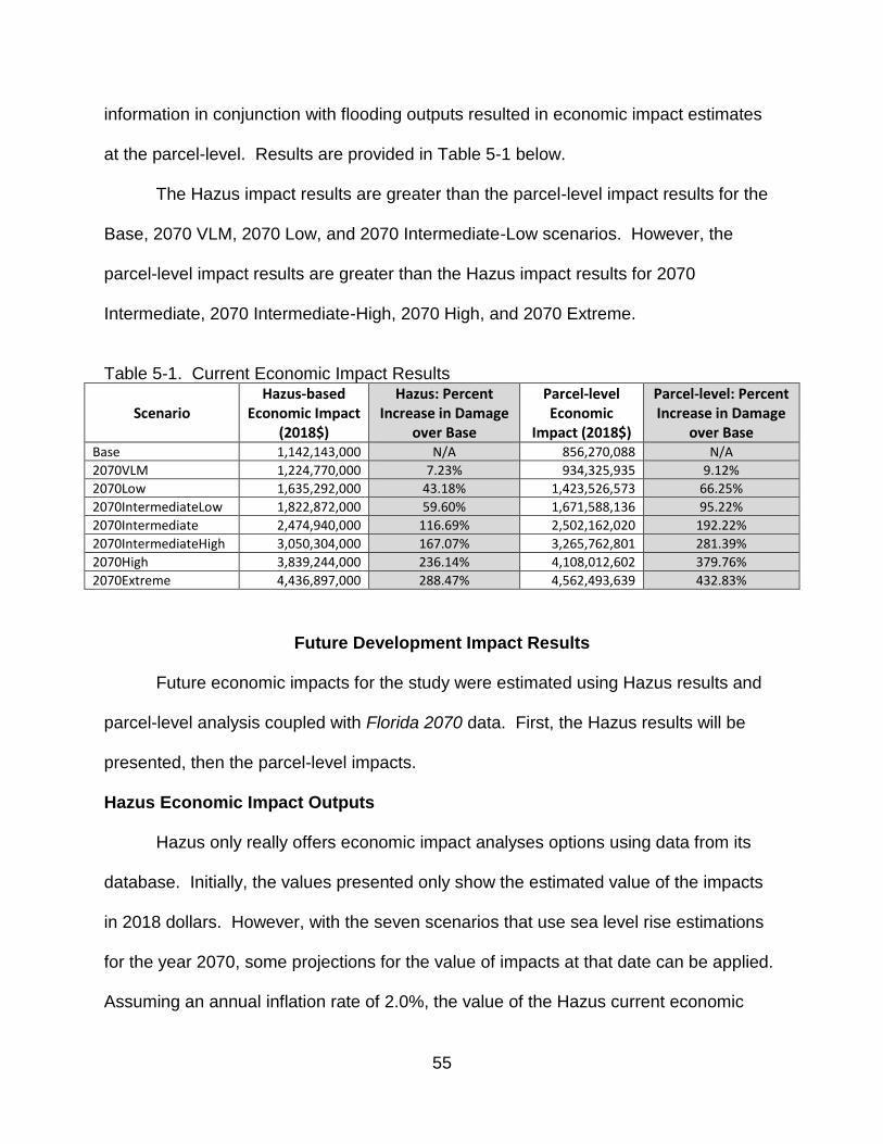
selecting a few options for what to include in the economic impact analysis. Results are

provided in Table 5-1 below.

Parcel-level Economic Impact Outputs

The parcel-level economic impact analysis was conducted to compare how using

finer detail in input data would affect economic impact outcomes. The parcel-level

analysis used data from the St. Johns County Property Appraiser and flooding outputs

from Hazus to calculate impact estimates. Parcels were assigned a depth-damage

curve from the Hazus database based on the land-use and building type. Using this

55

information in conjunction with flooding outputs resulted in economic impact estimates

at the parcel-level. Results are provided in Table 5-1 below.

The Hazus impact results are greater than the parcel-level impact results for the

Base, 2070 VLM, 2070 Low, and 2070 Intermediate-Low scenarios. However, the

parcel-level impact results are greater than the Hazus impact results for 2070

Intermediate, 2070 Intermediate-High, 2070 High, and 2070 Extreme.

Table 5-1. Current Economic Impact Results

Scenario Hazus-based

Economic Impact (2018$)

Hazus: Percent Increase in Damage

over Base

Parcel-level Economic

Impact (2018$)

Parcel-level: Percent Increase in Damage

over Base Base 1,142,143,000 N/A 856,270,088 N/A

2070VLM 1,224,770,000 7.23% 934,325,935 9.12%

2070Low 1,635,292,000 43.18% 1,423,526,573 66.25%

2070IntermediateLow 1,822,872,000 59.60% 1,671,588,136 95.22%

2070Intermediate 2,474,940,000 116.69% 2,502,162,020 192.22%

2070IntermediateHigh 3,050,304,000 167.07% 3,265,762,801 281.39%

2070High 3,839,244,000 236.14% 4,108,012,602 379.76%

2070Extreme 4,436,897,000 288.47% 4,562,493,639 432.83%

Future Development Impact Results

Future economic impacts for the study were estimated using Hazus results and

parcel-level analysis coupled with Florida 2070 data. First, the Hazus results will be

presented, then the parcel-level impacts.

Hazus Economic Impact Outputs

Hazus only really offers economic impact analyses options using data from its

database. Initially, the values presented only show the estimated value of the impacts

in 2018 dollars. However, with the seven scenarios that use sea level rise estimations

for the year 2070, some projections for the value of impacts at that date can be applied.

Assuming an annual inflation rate of 2.0%, the value of the Hazus current economic

56

impact results, presented in the previously, can be calculated for the year 2070. The

results are shown in Table 5-2 below.

Parcel-level Economic Impact Outputs

Similar to the Hazus outputs, the seven parcel-level impact outputs that included

sea level rise estimations in 2070 initially only present impact estimations in 2018

dollars. Using the same annual inflation rate, 2.0%, the value of these impacts can be

projected for 2070. The results are shown in Table 5-2 below.

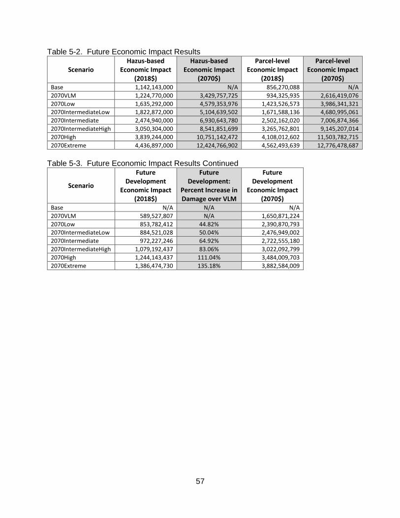
More significantly, future economic impacts have been calculated for areas

projected to be developed by the Florida 2070 project. In these areas slated for new

development, a ratio of land-use/building types from currently developed parcels was

used to forecast the makeup of the projected developed lands in 2070. Using this

information, valuation of these land-uses per square foot, the area of the future

developed areas inundated by coastal flooding, and the average flood depth for each

scenario the estimated economic impact to future development in 2070 from coastal

flooding events with additional sea level rise could be calculated. These values are

presented in Table 5-3 below in both 2018 and 2070 dollars.

Future development impact results show that from $1.6 billion to nearly $4 billion

(2070$) of additional property may be impacted by coastal flooding in 2070 if current

development continues in a similar pattern. This increases vulnerability by about 30%

to 60%, depending on the flooding scenario.

57

Table 5-2. Future Economic Impact Results

Scenario Hazus-based

Economic Impact (2018$)

Hazus-based Economic Impact

(2070$)

Parcel-level Economic Impact

(2018$)

Parcel-level Economic Impact

(2070$) Base 1,142,143,000 N/A 856,270,088 N/A

2070VLM 1,224,770,000 3,429,757,725 934,325,935 2,616,419,076

2070Low 1,635,292,000 4,579,353,976 1,423,526,573 3,986,341,321

2070IntermediateLow 1,822,872,000 5,104,639,502 1,671,588,136 4,680,995,061

2070Intermediate 2,474,940,000 6,930,643,780 2,502,162,020 7,006,874,366

2070IntermediateHigh 3,050,304,000 8,541,851,699 3,265,762,801 9,145,207,014

2070High 3,839,244,000 10,751,142,472 4,108,012,602 11,503,782,715

2070Extreme 4,436,897,000 12,424,766,902 4,562,493,639 12,776,478,687

Table 5-3. Future Economic Impact Results Continued

Scenario

Future Development

Economic Impact (2018$)

Future Development:

Percent Increase in Damage over VLM

Future Development

Economic Impact (2070$)

Base N/A N/A N/A

2070VLM 589,527,807 N/A 1,650,871,224

2070Low 853,782,412 44.82% 2,390,870,793

2070IntermediateLow 884,521,028 50.04% 2,476,949,002

2070Intermediate 972,227,246 64.92% 2,722,555,180

2070IntermediateHigh 1,079,192,437 83.06% 3,022,092,799

2070High 1,244,143,437 111.04% 3,484,009,703

2070Extreme 1,386,474,730 135.18% 3,882,584,009

58

CHAPTER 6 DISCUSSION AND CONCLUSION

Discussion of the outcomes from the coastal flooding analysis and economic

impact analysis is found below. Conclusions from the outcomes are drawn and

limitations are elaborated on, as well as opportunities for further research.

Coastal Flooding from Base 100-Year Storm and Impacts

Considering the vulnerability to a coastal flooding event in St. Johns County and

estimated economic impacts, the coastal flooding analysis shows how a 100-year storm

could impact St. Johns County. Figure 6-1 and 6-2 presents the flooding that coastal

areas in the county may experience in the event of a 100-year storm. In addition to

some flooding on the beaches, extensive flooding can be seen along the Matanzas,

Guana, and Tolomato Rivers as well as along the Intracoastal Waterway. In many

cases, it is the low-lying areas close to the river mouths and along the river runs that are

most vulnerable to flooding. This is somewhat counter-intuitive because coastal

flooding events caused by hurricanes are generally expected to have the greatest

impact on properties on or near the beach. However, the extensive dune system and

slightly higher elevations found near the coastline reduces the vulnerability of these

areas to flooding. The lower elevation of land along the rivers exposes them to greater

flooding risk. Storm surge pushing water through inlets and up the rivers can impact

many properties in these lower-elevation areas.

With this flooding vulnerability in mind, a 100-year storm with no sea level rise is

estimated to flood nearly 40,000 acres of land in St. Johns County. This translates to

about $1.1 billion of damage to buildings in the Hazus impact model and about $850

million of damage to buildings in the parcel-level impact model. The reason for this

59

difference is tied to the method for calculating impacts in each model. Hazus, because

it is built for use anywhere in the US, can only predict economic impacts from flooding at

the Census Block level. As a result, more specific information about building valuation

and the impacts that certain parcels experience from flooding are lost in data

aggregation. However, at the parcel level, these specifics are not lost. They are

factored into the overall model, taking into account valuations for individual properties

and their location across a Census Block. By limiting aggregation and considering

parcel-level impacts, the parcel-level model minimizes generalization and gives a more

accurate estimation of flooding impacts on buildings. It is also important to note that the

Hazus database of building information is not as current as the parcel data used. This

also helps explain discrepancies between the two impact estimations. Additionally, this

impact is only to buildings in the study area and does include any other infrastructure.

60

Figure 6-1. Hazus Coastal Flooding Output – Base Flooding Scenario for St. Johns County

61

Figure 6-2. Hazus Coastal Flooding Output – Base Flooding Scenario in the St. Augustine Area

62

Coastal Flooding from 100-Year Storms with Extra Sea Level Rise and Impacts

Seven sea level rise scenarios were modeled to show a range of sea level rise

increases and coastal flooding events may impact St. Johns County in the future. It is

clear that coastal flooding events with additional sea level rise will have a major impact.

At the lowest sea level rise scenario, 2070 VLM, 0.13 feet of sea level rise translates to

about 41,000 acres of land being inundated by a 100-year storm event, 1000 acres

more than the Base event. In the 2070 Extreme scenario, nearly five and a half feet of

sea level rise coupled with a 100-year storm event is estimated to flood nearly 58,000

acres of land, about 18,000 more than the base scenario. More specifics for the various

100-year storm scenarios can be seen in Table 4-1 in Chapter 4. Figures 6-3 and 6-4

show the extent of flooding in St. Johns County for the 2070 VLM and 2070 Extreme

scenarios, respectively. All maps of the various coastal flooding scenarios can be seen

in Appendix C.

The economic impacts are also projected to increase with additional sea level

rise. For the Hazus model, impacts to buildings range from $3.4 to $12.4 billion in 2070

dollars. For the parcel-level model, impacts to buildings range from $2.6 to $12.7 billion

in 2070 dollars. Curiously, there is a point where impacts modeled in the parcel-level

analysis overtake the impacts modeled in the Hazus analysis. From the Base scenario

to the 2070 Intermediate-Low scenario, Hazus predicts greater impacts to buildings than

the parcel-level analysis. However, from the 2070 Intermediate scenario to the 2070

Extreme scenario, the parcel-level analysis predicts greater impacts to buildings than

Hazus. Though half of the scenarios follow expectations, the scenarios with larger

amounts of sea level rise do not. This may be for a variety of reasons, however there

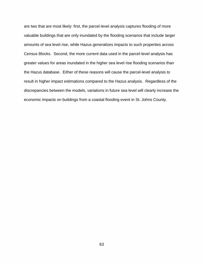
63

are two that are most likely: first, the parcel-level analysis captures flooding of more

valuable buildings that are only inundated by the flooding scenarios that include larger

amounts of sea level rise, while Hazus generalizes impacts to such properties across

Census Blocks. Second, the more current data used in the parcel-level analysis has

greater values for areas inundated in the higher sea level rise flooding scenarios than

the Hazus database. Either of these reasons will cause the parcel-level analysis to

result in higher impact estimations compared to the Hazus analysis. Regardless of the

discrepancies between the models, variations in future sea level will clearly increase the

economic impacts on buildings from a coastal flooding event in St. Johns County.

64

Figure 6-3. Hazus Coastal Flooding Output – 2070 VLM Flooding Scenario for St. Johns County

65

Figure 6-4. Hazus Coastal Flooding Output – 2070 Extreme Flooding Scenario for St. Johns County

66

Coastal Flooding Impacts on Future Development

Future development in St. Johns County, projected by the Florida 2070 study,

was overlaid with the various coastal flooding scenarios including sea level rise. Of the

almost 180,000 acres of land projected to be developed in the 2070 Trend scenario,

between about 4,000 and 7,200 acres was estimated to be inundated by the various

coastal flooding scenarios. With this information, it was possible to calculate the

estimated economic impact to buildings in the future developed areas. Again, only

impacts to buildings were included in the analysis, no other infrastructure was

considered. It was estimated coastal flooding would cause between $1.6 and $3.9

billion in damage to buildings.

Though only between about 2% to 5% of the total area projected to be developed

would be inundated, it would add significantly to the impacts of a coastal flooding event

in St. Johns County. Figures 6-5 and 6-6 below show examples of the flooding impacts

to future developed areas and Table 5-2 and 5-3 in Chapter 5 show dollar values of the

impacts.

A key consideration of this part of the analysis is how the 2070 Trend future

development area was broken up into different land use/building type categories. The

technique of using the land use breakdown for future development derived from the

parcels used in the parcel-level analysis is the most logical method. The current

development pattern can be projected into the future to represent the trend of

development. Beyond this method, it is difficult to estimate building values with any

strong theoretical basis that far into the future. There are long-range development

plans, such as county comprehensive plans which lay out future land use, but these

67

typically extend no more than 30 years into the future. Using current development

patterns, for which there is building valuation information, permits the estimation of

future development values.

Also keep in mind that the location of future development may be in

somewhat risky locations. In the scenarios with more dramatic sea level rise, local

governments and regulatory agencies may be more hesitant to permit building in low-

lying areas. As a result, the future economic impacts may be overestimated. However,

it is difficult to judge and properly model the combination of factors affecting future

development trends at this level. Simply continuing trends into the future generate

useful outputs that can be used as a baseline

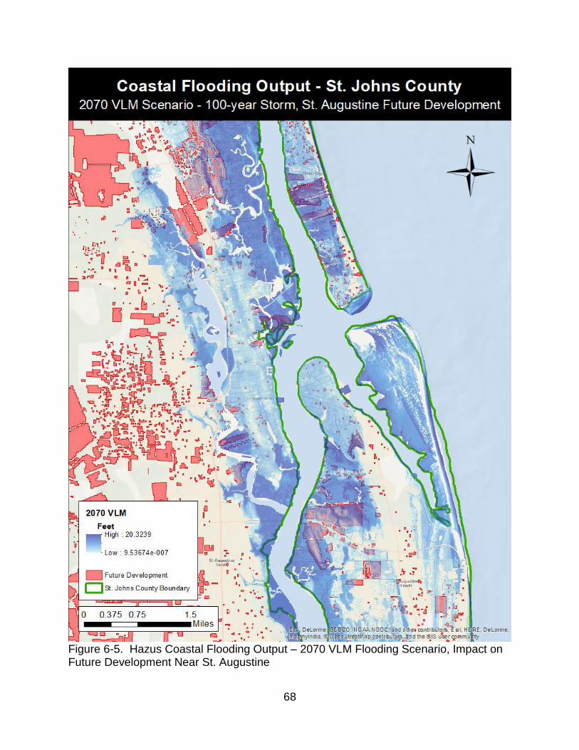
68

Figure 6-5. Hazus Coastal Flooding Output – 2070 VLM Flooding Scenario, Impact on Future Development Near St. Augustine

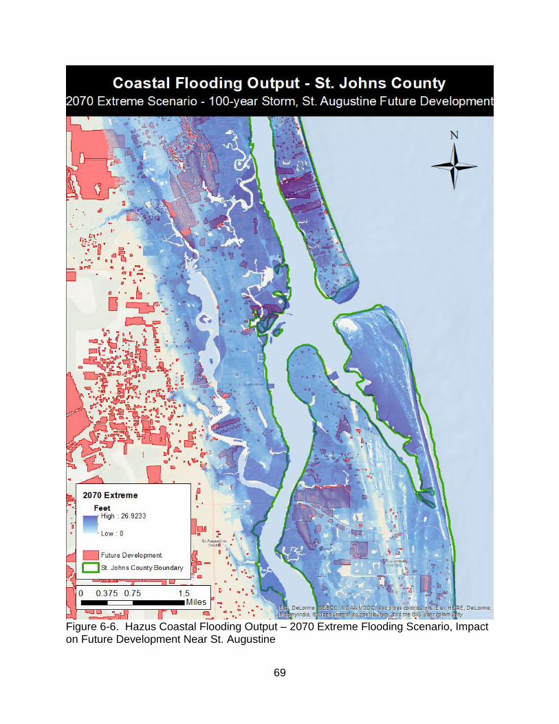
69

Figure 6-6. Hazus Coastal Flooding Output – 2070 Extreme Flooding Scenario, Impact on Future Development Near St. Augustine

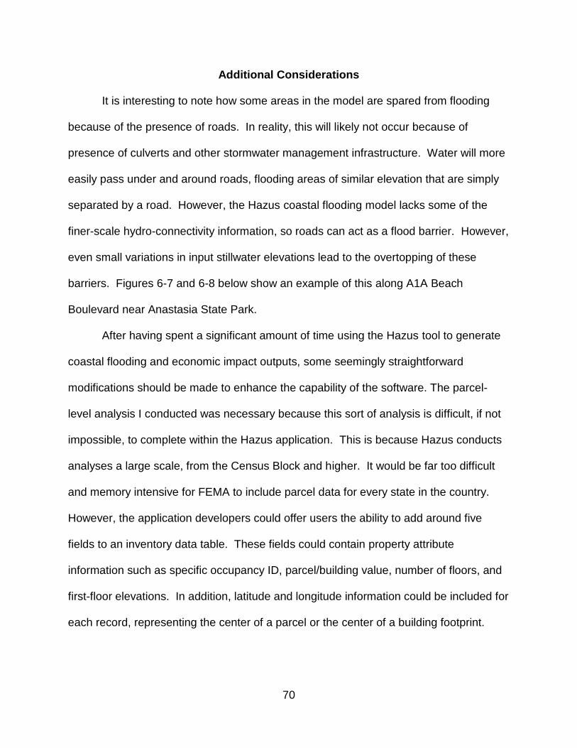
70

Additional Considerations

It is interesting to note how some areas in the model are spared from flooding

because of the presence of roads. In reality, this will likely not occur because of

presence of culverts and other stormwater management infrastructure. Water will more

easily pass under and around roads, flooding areas of similar elevation that are simply

separated by a road. However, the Hazus coastal flooding model lacks some of the

finer-scale hydro-connectivity information, so roads can act as a flood barrier. However,

even small variations in input stillwater elevations lead to the overtopping of these

barriers. Figures 6-7 and 6-8 below show an example of this along A1A Beach

Boulevard near Anastasia State Park.

After having spent a significant amount of time using the Hazus tool to generate

coastal flooding and economic impact outputs, some seemingly straightforward

modifications should be made to enhance the capability of the software. The parcel-

level analysis I conducted was necessary because this sort of analysis is difficult, if not

impossible, to complete within the Hazus application. This is because Hazus conducts

analyses a large scale, from the Census Block and higher. It would be far too difficult

and memory intensive for FEMA to include parcel data for every state in the country.

However, the application developers could offer users the ability to add around five

fields to an inventory data table. These fields could contain property attribute

information such as specific occupancy ID, parcel/building value, number of floors, and

first-floor elevations. In addition, latitude and longitude information could be included for

each record, representing the center of a parcel or the center of a building footprint.

71

With this information entered, a user would be able to produce economic impact

outputs specific to their location within the Hazus tool. Creating a model in Model

Builder or python script to use these fields as inputs and generate impact outputs would

be straightforward. Overlaying this information within the Hazus tool would streamline

the process and reduce the potential for errors when trying to get more specific impact

estimates.

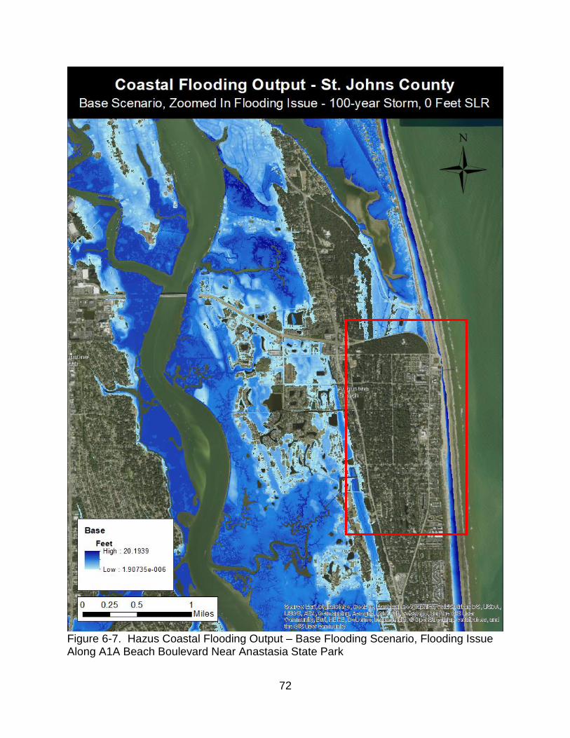
72

Figure 6-7. Hazus Coastal Flooding Output – Base Flooding Scenario, Flooding Issue Along A1A Beach Boulevard Near Anastasia State Park

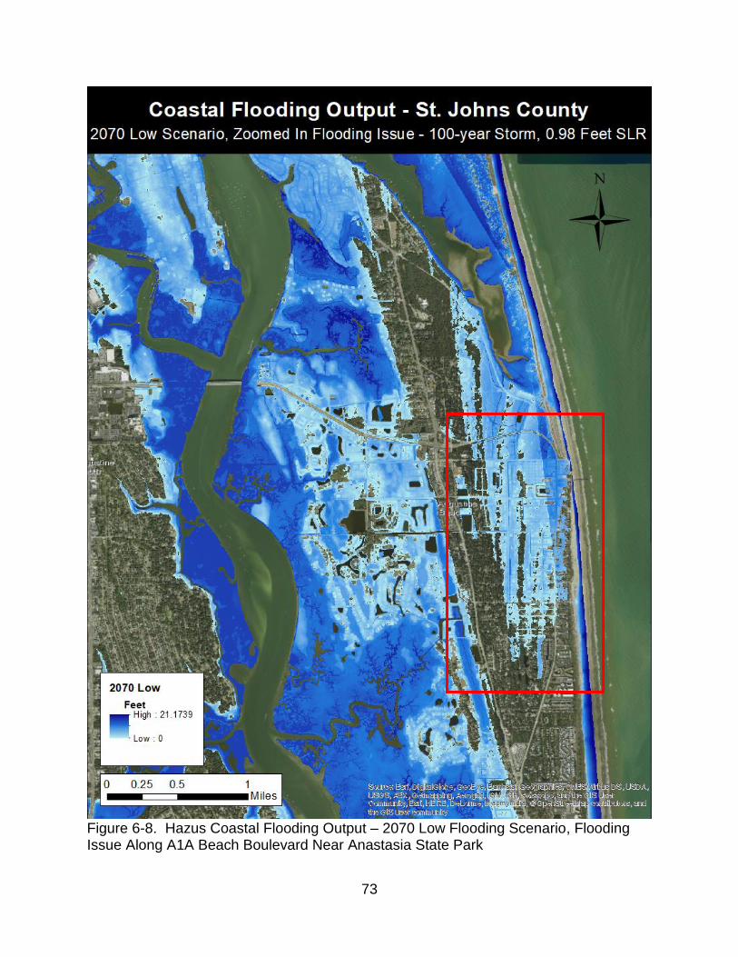
73

Figure 6-8. Hazus Coastal Flooding Output – 2070 Low Flooding Scenario, Flooding Issue Along A1A Beach Boulevard Near Anastasia State Park

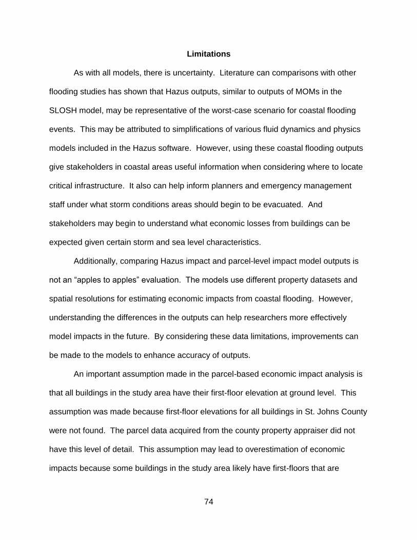
74

Limitations

As with all models, there is uncertainty. Literature can comparisons with other

flooding studies has shown that Hazus outputs, similar to outputs of MOMs in the

SLOSH model, may be representative of the worst-case scenario for coastal flooding

events. This may be attributed to simplifications of various fluid dynamics and physics

models included in the Hazus software. However, using these coastal flooding outputs

give stakeholders in coastal areas useful information when considering where to locate

critical infrastructure. It also can help inform planners and emergency management

staff under what storm conditions areas should begin to be evacuated. And

stakeholders may begin to understand what economic losses from buildings can be

expected given certain storm and sea level characteristics.

Additionally, comparing Hazus impact and parcel-level impact model outputs is

not an “apples to apples” evaluation. The models use different property datasets and

spatial resolutions for estimating economic impacts from coastal flooding. However,

understanding the differences in the outputs can help researchers more effectively

model impacts in the future. By considering these data limitations, improvements can

be made to the models to enhance accuracy of outputs.

An important assumption made in the parcel-based economic impact analysis is

that all buildings in the study area have their first-floor elevation at ground level. This

assumption was made because first-floor elevations for all buildings in St. Johns County

were not found. The parcel data acquired from the county property appraiser did not

have this level of detail. This assumption may lead to overestimation of economic

impacts because some buildings in the study area likely have first-floors that are

75

elevated. Buildings with first floor elevations above ground level will face lower risk to

flooding damage and see lower economic losses in the event of a flood. However, until

more information is available for first-floor elevations of buildings across St. Johns

County, assuming ground level first-floor elevations provides a standardized method in

the analysis process. Property appraisers, especially in counties facing major flooding

risks, could begin compiling first-floor elevation information for properties. Maintaining

this information would supply risk managers and planners with a valuable resource to

better understand vulnerabilities to flooding.

Using only the value of buildings on a parcel as a proxy for economic impacts

from a coastal flooding event can lead to additional underestimations of estimated

impacts. Using only building values does not include any valuation of the land on which

the building sits. The value of the buildings plus the value of the land determines the

taxable value of the parcel, which determines a significant portion the property tax base

for local governments. If these combined values are permanently impacted by a coastal

flooding event and/or sea level rise, local governments will face losses to their tax base

on top of having to manage other impacts from these hazards. Other analyses can be

conducted where the taxable value of a parcel is used, rather than just the building

value, to give local officials an idea of how they may be impacted by coastal flooding

and sea level rise. Looking into the potential permanent loss of income from property

taxes will show additional vulnerability of a community to hazards.

Suggestions for Future Research

Future research efforts can be made to increase the resolution of the impact

analysis. Specifically, the methods used in the parcel-level analysis can be narrowed

76

further, so that flooding on building footprints is analyzed. Focusing the flooding

impacts even further should help create an even more accurate estimate of the impacts

from flooding on buildings. However, this effort would be very intensive. The process of

creating building footprints for an entire county would require major investments of time

and money to produce a high-quality result.

This research only focused on coastal flooding and sea level rise on the eastern

side of St. Johns County, which is bordered by the Atlantic Ocean. However, further

flooding analysis should be conducted on the western side of the county which is

bordered by the St. Johns River. The St. Johns River in this area may not be exposed

to as significant storm surge effects, but sea level rise will certainly have an impact on

the western side of the county. To get a complete picture of how St. Johns County may

be impacted by coastal flooding and sea level rise, the western side of the county

should be included in future research.

In addition to using Hazus as the sole model to produce coastal flooding outputs,

other models, like those mentioned in Chapter 2, could be used to create alternative

flooding scenarios. Other models that require greater technical knowledge may be able

to produce more representative flooding outputs and, therefore, could give a more

realistic idea of how a 100-year coastal flooding event may impact St. Johns County.

Finally, estimating the impacts of coastal flooding events on infrastructure

beyond buildings, like the transportation network, can give stakeholders a more

complete view of how coastal flooding events may impact their community. Buildings

area significant piece of the fabric of communities and represent major assets for

77

individuals and organizations, but they are not the only infrastructure impacted by a

coastal flooding event.

Concluding Thoughts

It is clear that St. Johns County faces major flooding risk from strong hurricanes.

Furthermore, if development is allowed to continue in the future as it has leading up to

now, many more built-up areas will be vulnerable by 2070. It is in the best interest of

stakeholders around coastal areas to consider how they may be impacted by storm

surge right now and how the combination of storm surge and sea level rise may make

outcomes worse in the future.

An important step in working to minimize future vulnerabilities is to limit

development in low-lying areas near inlets and along the river and intracoastal. New

ordinances or codes preventing development in floodplains should be enacted to limit

this vulnerability. Further, implementing regulations that require buildings which were

catastrophically damaged by a flooding event to be reconstructed with enhanced

structural qualities or higher first floor elevations will minimize the risk of repeated

damage to a single property. If development in risky areas cannot be curtailed, then

imposing certain criteria for new development, such as establishing minimum first floor

elevations above estimated 100-year flood levels with an additional sea level rise value,

would be a way to help mitigate vulnerability.

If steps are not taken by local governments to curtail unwise development in the

future, they may be exposing themselves to major legal and financial risk. An example

can be seen in the Jordan et al. v St. Johns County 2011 case. If a local government

permits development and serves that development with utility or transportation

78

infrastructure, that entity is responsible with maintaining the original level of service

provided to the development. In the face of more frequent severe storms and sea level

rise, this could be an ultimately bankrupting proposition in the long run as maintenance

costs progressively rise. Other legal issues may arise if landowners decide to abandon

their property in the face of storms and sea level rise which renders their property

ultimately worthless. It is unclear who would be responsible for managing physical and

environmental risks posed by derelict buildings slowly becoming inundated by rising

seas and ripped apart by storms.

Coastal areas around Florida, the US, and the world are vulnerable to storm

surge and sea level rise. In the future these vulnerabilities are likely to increase as

areas continue to develop and as risks of more powerful storms and rising seas

increase. It is important for communities to understand these risks and how they

expose infrastructure in their area to damage. Modeling the physical and economic

impacts of current coastal flooding events and future events coupled with sea level rise

can help communities better understand current and future vulnerabilities. Moving

forward leaders can use this information to take steps to minimize potential impacts and

increase the resiliency of their communities.

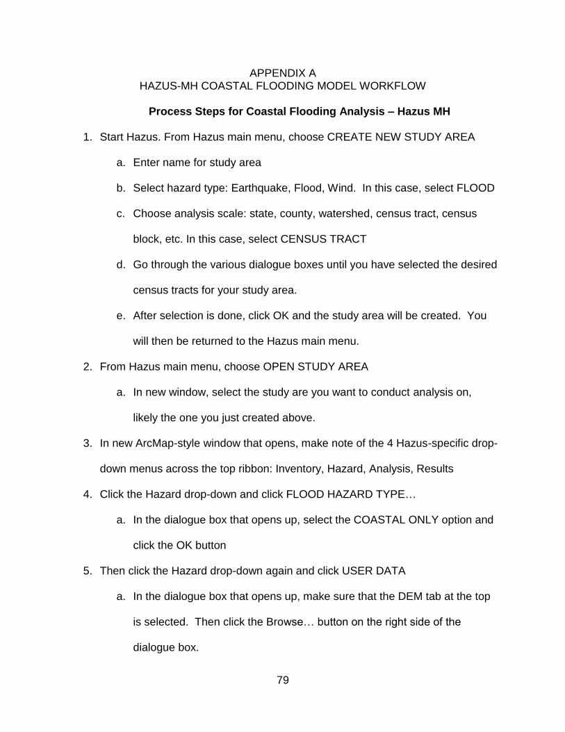
79

APPENDIX A HAZUS-MH COASTAL FLOODING MODEL WORKFLOW

Process Steps for Coastal Flooding Analysis – Hazus MH

1. Start Hazus. From Hazus main menu, choose CREATE NEW STUDY AREA

a. Enter name for study area

b. Select hazard type: Earthquake, Flood, Wind. In this case, select FLOOD

c. Choose analysis scale: state, county, watershed, census tract, census

block, etc. In this case, select CENSUS TRACT

d. Go through the various dialogue boxes until you have selected the desired

census tracts for your study area.

e. After selection is done, click OK and the study area will be created. You

will then be returned to the Hazus main menu.

2. From Hazus main menu, choose OPEN STUDY AREA

a. In new window, select the study are you want to conduct analysis on,

likely the one you just created above.

3. In new ArcMap-style window that opens, make note of the 4 Hazus-specific drop-

down menus across the top ribbon: Inventory, Hazard, Analysis, Results

4. Click the Hazard drop-down and click FLOOD HAZARD TYPE…

a. In the dialogue box that opens up, select the COASTAL ONLY option and

click the OK button

5. Then click the Hazard drop-down again and click USER DATA

a. In the dialogue box that opens up, make sure that the DEM tab at the top

is selected. Then click the Browse… button on the right side of the

dialogue box.

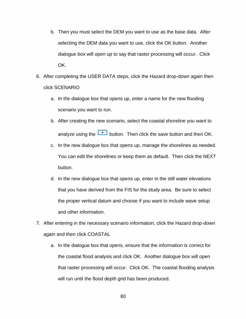
80

b. Then you must select the DEM you want to use as the base data. After

selecting the DEM data you want to use, click the OK button. Another

dialogue box will open up to say that raster processing will occur. Click

OK.

6. After completing the USER DATA steps, click the Hazard drop-down again then

click SCENARIO

a. In the dialogue box that opens up, enter a name for the new flooding

scenario you want to run.

b. After creating the new scenario, select the coastal shoreline you want to

analyze using the button. Then click the save button and then OK.

c. In the new dialogue box that opens up, manage the shorelines as needed.

You can edit the shorelines or keep them as default. Then click the NEXT

button.

d. In the new dialogue box that opens up, enter in the still water elevations

that you have derived from the FIS for the study area. Be sure to select

the proper vertical datum and choose if you want to include wave setup

and other information.

7. After entering in the necessary scenario information, click the Hazard drop-down

again and then click COASTAL

a. In the dialogue box that opens, ensure that the information is correct for

the coastal flood analysis and click OK. Another dialogue box will open

that raster processing will occur. Click OK. The coastal flooding analysis

will run until the flood depth grid has been produced.

81

8. After the process is completed, the depth grid will be produced

82

APPENDIX B ECONOMIC IMPACT ANALYSIS WORKFLOW

Current Development Parcel-Level Economic Impact Analysis Steps

After downloading parcel data and property data, in the form of CAMA files,

from the St. Johns County Property Appraiser, the data had to be processed and

reorganized to facilitate data analysis. The following steps describe in detail the

steps taken to reorganize the data.

1. Parcel data from the St. Johns Property Appraiser came in an ArcGIS file

geodatabase. Within the file geodatabase, a single parcel feature class was

present containing all of the parcel boundaries and limited descriptive data for

each parcel. The projected coordinate system of the data originally was

NAD_1983_StatePlane_Florida_East_FIPS_0901_Feet. However, to match the

coordinate system of the various flood depth grids, the parcel data was re-

projected to NAD_1983_UTM_Zone_17N. The new parcel layer was named

“parcels_projected” and was used later.

2. Next, the CAMA files were processed. The CAMA files came in the form of

Microsoft Access Databases, with multiple tables found within each database.

Two CAMA databases were downloaded, “CamaData” and “CamaDataSup”.

These databases contained property information such as parcel values, building

values, and building structural information.

a. Three tables were taken from the two access databases and converted

into excel files: ParcelView, BldView, and StructElemView.

b. These three excel files were then converted into file geodatabase tables in

ArcGIS using the “Excel to Table” tool in ArcMap.

83

3. After converting the tables to file geodatabase tables, the data was cleaned to

remove unnecessary records and attribute information.

a. The ParcelView table contained a field offering information about the total

value of buildings on the parcel called “tot_bld_val”. Any parcels which

had no buildings, or no building value, were not included in the analysis.

Records with tot_bld_val equal to zero were removed from the dataset by

selecting records which had building values greater than zero and

exporting these records into a new table called

“parcelview_data_bldval_notzero”.

b. The StructElemView table contained information describing building

specifications based on parcel number, with multiple records for a single

parcel. One of the records contained information on the number of stories

for each building. These records were selected and exported to a new

table called “structelemunit_storiesonly”.

c. No extra processing was required for the BldView table.

4. After cleaning the data tables, they could be joined. First, the

“parcelview_data_bldval_notzero” and the BldView tables were joined using the

“Strap” field, a field containing a unique identifier for each parcel in the county.

The joined tables were exported to a new table called “parcel_bld_join”.

5. Next, the structelemunit_storiesonly table was joined with the parcel_bld_join

table using the strap field as the join field. The joined tables were exported to a

new table called “parcel_bld_struct_join”.

84

6. The parcel_bld_struct_join table was joined to the parcels_projected feature

class. The Strap field was used as the join field. The joined feature class was

exported to preserve the join and was renamed “parcels_processed”

7. Finally, the “tot_bld_val” field in the parcels_processed layer was queried so that

only parcels with a tot_bld_val greater than zero was selected. This selection

was exported to a new feature class called “parcels_bldval”

After cleaning and reorganizing the parcel and property data, the flood depth

grids had to be processed to ensure that only areas that needed to be analyzed

were in the flood depth grid boundaries. This was accomplished by using land

use and land cover data from St. Johns River Water Management District,

supplied by the Florida Geographic Data Library (FGDL).

8. The layer named “lu_sjrwmd_2009_feb12” was downloaded from FGDL

9. The lu_sjrwmd_2009_feb12 was then project from the FGDL Albers projection to

UTM_17N using the project tool to match the flood depth grid layers. The

projected layer was called lu_sjrwmd_2009_feb12_utm.

10. The lu_sjrwmd_2009_feb12_utm layer then needed to be narrowed to the study

area, so a select by location operation was done using the St. Johns county

boundary. If any part of the lu_sjrwmd_2009_feb12_utm layer intersected the

county boundary, it was selected. The selected features from the

lu_sjrwmd_2009_feb12_utm layer were exported to a new layer called

lu_sjrwmd_2009_feb12_utm_stjohncnty.

11. The lu_sjrwmd_2009_feb12_utm_stjohncnty layer was then selected by attribute

using a specific string. The selection was made to select open water areas and

85

then remove them so that a land only layer could be used to mask flood depth

grids. The selection string used can be seen below:

a. "LCCOD_DESC" = '9999: MISSING LUCODE OR OUTSIDE SJRWMD'

OR "LCCOD_DESC" = '8370: SURFACE WATER COLLECTION BASINS'

OR "LCCOD_DESC" = '5100: STREAMS AND WATERWAYS' OR

"LCCOD_DESC" = '5200: LAKES' OR "LCCOD_DESC" = '5300:

RESERVOIRS - PITS, RETENTION PONDS, DAMS' OR

"LCCOD_DESC" = '5400: BAYS AND ESTUARIES' OR "LUCOD_DESC"

= '8370: SURFACE WATER COLLECTION BASINS' OR "LCCOD_DESC"

= '5250: OPEN WATER WITHIN A FRESHWATER MARSH / MARSHY

LAKES' OR "LCCOD_DESC" = '5430: ENCLOSED SALTWATER PONDS

WITHIN A SALT MARSH'

b. After making the selection, the selection was switched and the

lu_sjrwmd_2009_feb12_utm_stjohncnty layer was exported. The new

layer was called lu_sjrwmd_2009_feb12_utm_watermask_final

12. The lu_sjrwmd_2009_feb12_utm_stjohncnty_watermask_final layer was then

used to mask out undesired water areas from the flood depth grids.

After cleaning and reorganizing the parcel and property data, the property data

could be processed further to add information, such Specific Occupancy ID and

depth damage curves, to be used in economic impact analyses.

13. The field “SpecificOccID” field was added. Then, based on the land use, building

information, and number of stories, the Specific Occupancy was calculated. The

attribute information in this field is coordinated with attributes from the depth

86

damage curves to ensure that information from the depth damage curves can be

added to the parcel information.

14. A join was executed between the combined depth damage curves, derived from

the Hazus data, and the parcel information. The new “SpecificOccID” field from

the parcel layer was matched with a similar field in the depth damage curve layer

and the attribute information for the layers was matched. The layer was then

exported to make the join permanent.

Preparing flood information to determine flooded area of parcels

15. Flood depth rasters for each coastal flooding scenario that had been selected to

include only land areas were opened. These rasters were then converted to

integer rasters using the Int tool.

16. These new integer rasters were multiplied by zero using the Times tool.

17. The zero rasters were then converted to polygons.

18. The polygon flood boundaries then needed to be clipped to the parcels, so that

only the flooding in each parcel is considered. The Clip tool was used to isolate

the flooding polygons to only the parcel boundaries.

19. The clipped flood polygons then need to have their information added to the

parcel boundaries. This was done using the Intersect tool, but first a field called

“adam_area_sqft” was added to the parcels and Calculate Geometry wsa run to

determine the square foot area of the parcel. The Intersect tool was then run

once for each flood scenario polygon. Each intersected layer had a field added to

the output called “adam_base_fldarea” with base being replaced by the proper

87

flood scenario title. Calculate geometry was run for each field so the square feet

of flooding by scenario in each polygon was calculated.

20. After intersecting the parcels and the flood polygons, the resulting polygon layers

were spatial joined to the parcel layer, but only keeping the “adam_base_fldarea”

field (or similar field depending on the flooding scenario). In the spatial join tool,

the match option used was CONTAINS. These spatial joins were added on top of

prior spatial joins to produce a single parcel layer containing the flooded area

information for each parcel for each flooding scenario.

21. Finally, 8 fields were added. Each to serve as a location to calculate the

economic impact on a parcel for each flooding scenario.

Impact calculations

22. With the final parcel layer in hand, zonal statistics could be run for each flood

depth grid using the final parcel layer as the zone. The zonal statistics could then

be added to the parcel layer and the impact value calculated based on the

minimum flood depth in each parcel. Minimum flood depth was used to provide a

more conservative estimate of the flood impacts on a parcel.

88

Future Development Economic Impact Calculation Steps

Prep the Future Development Layer

1. First, load the following Florida 2070 datasets.

a. Florida2070_Dev_Base2010

b. Florida2070_Dev_Trend2070

c. Final parcel feature class used to calculate economic impact from flooding

d. St Johns County, the study area boundary

2. First, project the two Florida2070 layers into the coordinate system matching the

parcels feature class.

3. Next, clip the Trend2070 layer to the St Johns County boundary.

4. Next, erase the erased Trend2070 layer with the final parcels feature class.

5. Next, select only the features in the Trend2070 layer which have a DESCRIPT

equal to TREND2070. Export the selection to a new layer.

6. Next, dissolve the features in the most recent output layer so there is only one

record. Include as much information as you would like from the prior layer.

7. Add a field called “area_sqft” and Calculate Geometry for that field, calculating

the area in square feet for the Trend2070 feature.

8. The final output, call it Trend2070_Final, is the future development layer that can

be used to calculate future economic impact.

Calculate Flooding Depths for Impact Analysis

9. Use the polygon flood rasters created during the parcel level flooding analysis

and clip them to the Trend2070_Final layer.

89

10. Then, intersect each of those with the Trend2070_Final layer, creating 7

intersected feature classes. Then add a field to each of the intersected layers

with the title “adam_2070vlm_fldarea” with “2070vlm” being replaced by the

various flood scenario titles as necessary.

11. Next, spatial join these intersected layers to the Trend2070_Final feature class,

but only keeping the “adam_2070vlm_fldarea” field (or similar ones based on the

flood scenario). In the spatial join tool, the MATCH OPTION used was

INTERSECT. These spatial joins were added on top of prior spatial joins to

produce a single parcel layer containing all of the spatial information regarding

flooding extent in the future development area. The output is called

Trend2070_Final_spatialjoinFinal. Add 7 fields to serve as a location for

summing total impact value for each flooding scenario.

12. Using the Trend2070_Final_spatialjoinFinal layer, run zonal statistics on the flood

depth grids for the various 2070 flooding scenarios.

a. 2070vlm

b. 2070low

c. 2070intlow

d. 2070int

e. 2070inthigh

f. 2070high

g. 2070extreme

13. Then join all of these zonal stats tables to the spatialjoinFinal layer, so that each

flooding scenario has flood depth information in the table.

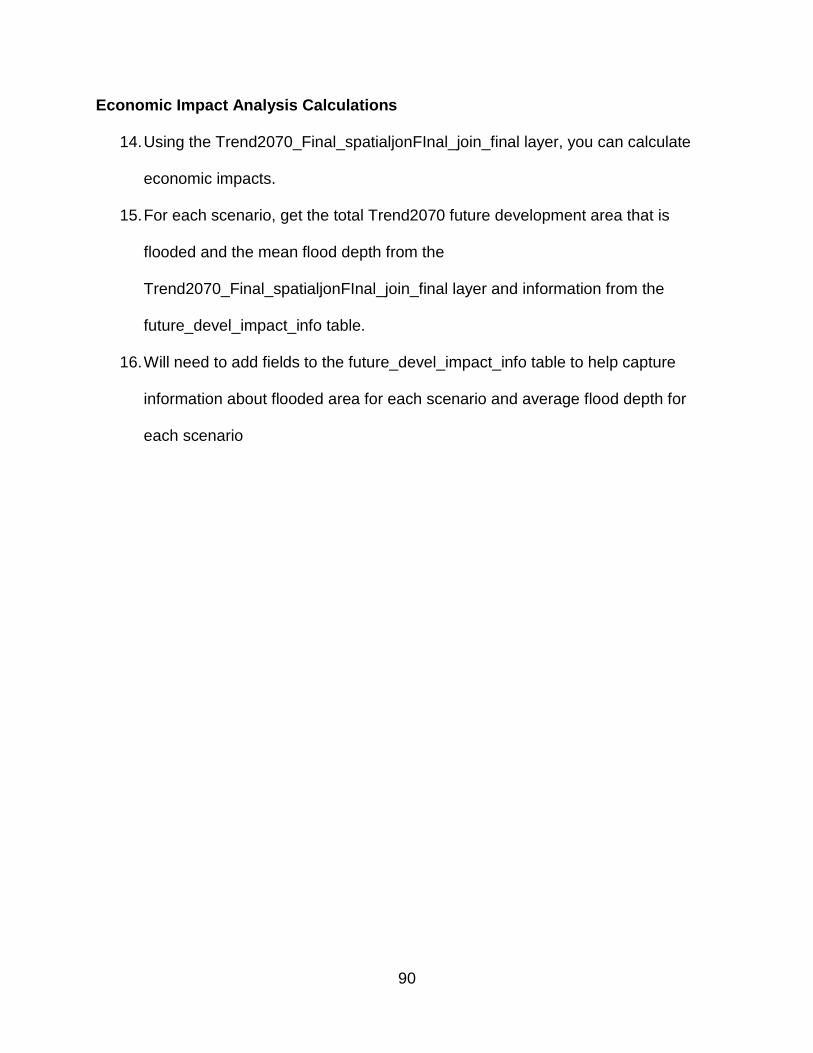
90

Economic Impact Analysis Calculations

14. Using the Trend2070_Final_spatialjonFInal_join_final layer, you can calculate

economic impacts.

15. For each scenario, get the total Trend2070 future development area that is

flooded and the mean flood depth from the

Trend2070_Final_spatialjonFInal_join_final layer and information from the

future_devel_impact_info table.

16. Will need to add fields to the future_devel_impact_info table to help capture

information about flooded area for each scenario and average flood depth for

each scenario

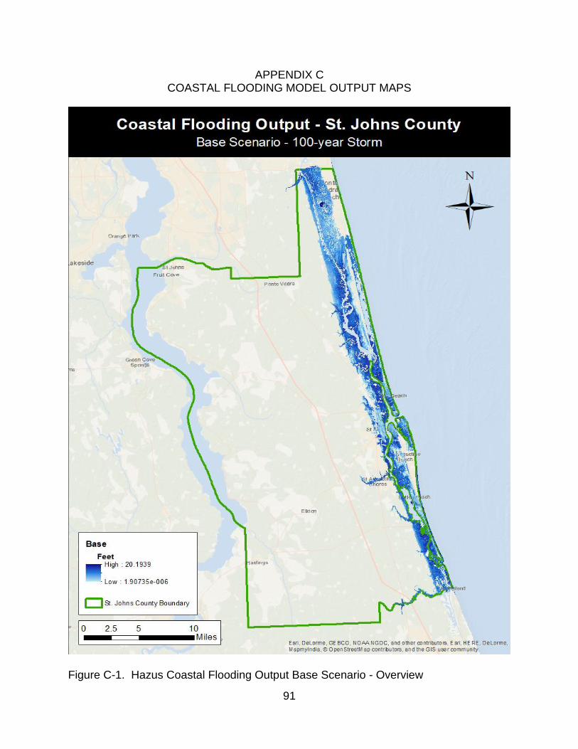
91

APPENDIX C COASTAL FLOODING MODEL OUTPUT MAPS

Figure C-1. Hazus Coastal Flooding Output Base Scenario - Overview

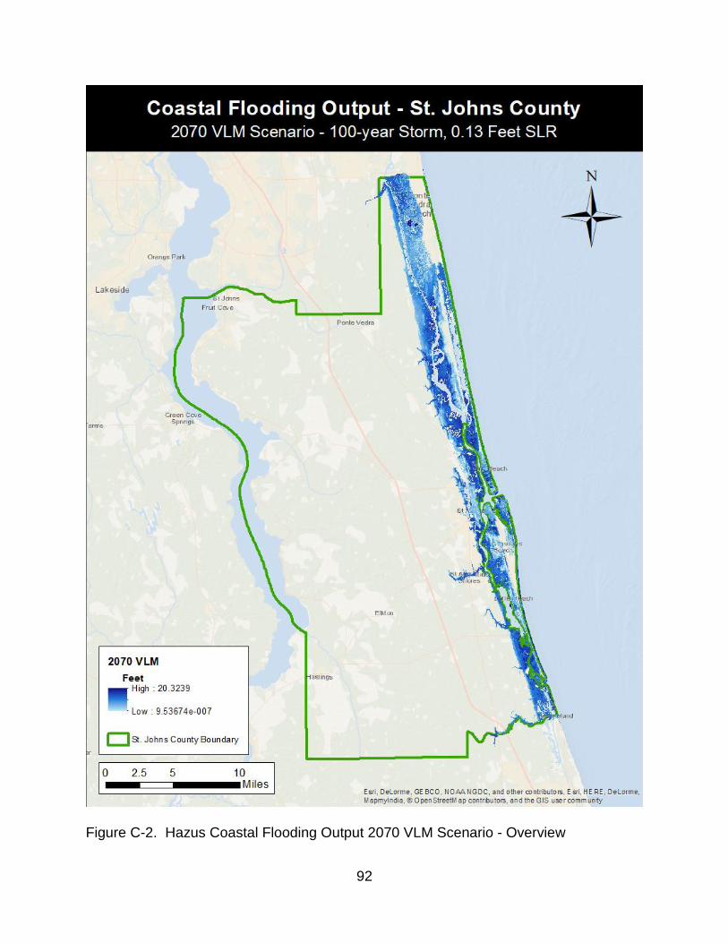
92

Figure C-2. Hazus Coastal Flooding Output 2070 VLM Scenario - Overview

93

Figure C-3. Hazus Coastal Flooding Output 2070 Low Scenario - Overview

94

Figure C-4. Hazus Coastal Flooding Output 2070 IntLow Scenario - Overview

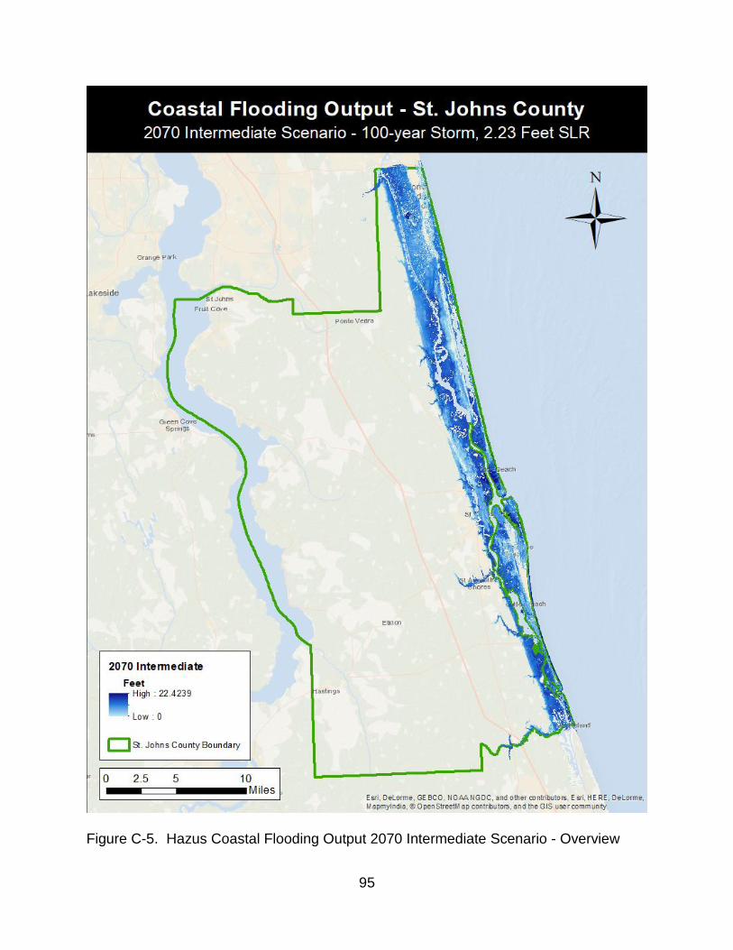
95

Figure C-5. Hazus Coastal Flooding Output 2070 Intermediate Scenario - Overview

96

Figure C-6. Hazus Coastal Flooding Output 2070 IntHigh Scenario - Overview

97

Figure C-7. Hazus Coastal Flooding Output 2070 High Scenario - Overview

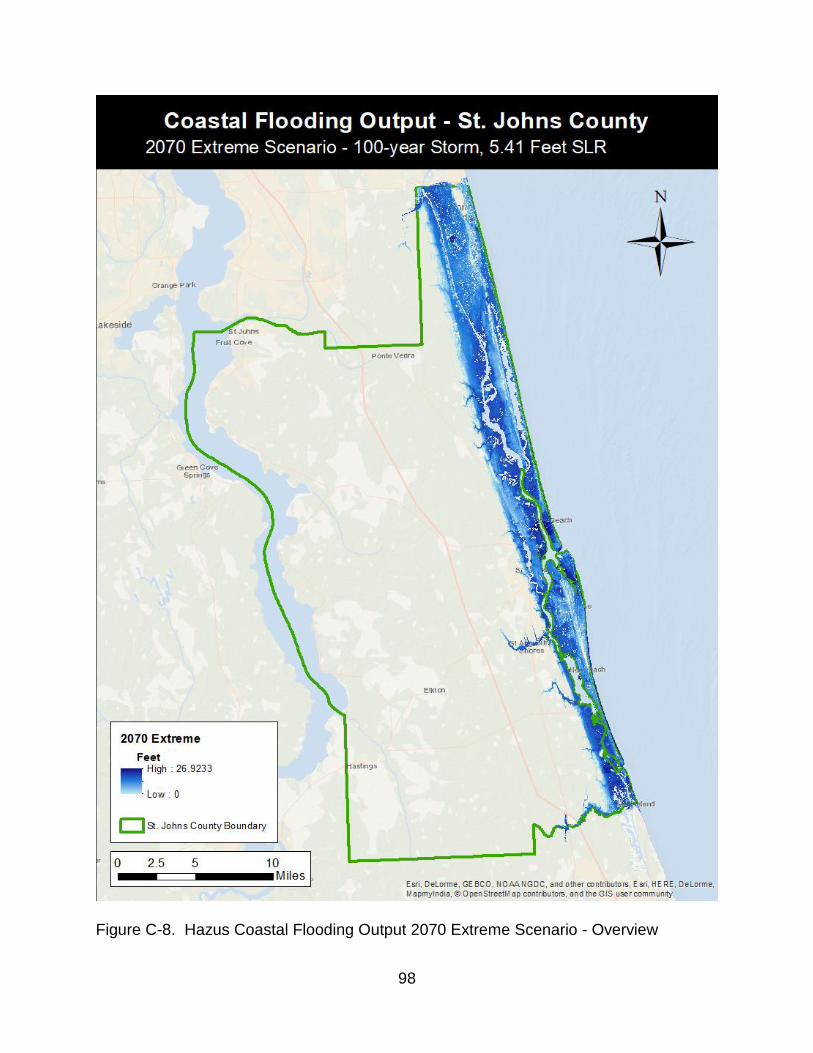
98

Figure C-8. Hazus Coastal Flooding Output 2070 Extreme Scenario - Overview

99

Figure C-9. Hazus Coastal Flooding Output Base Scenario – Zoomed In

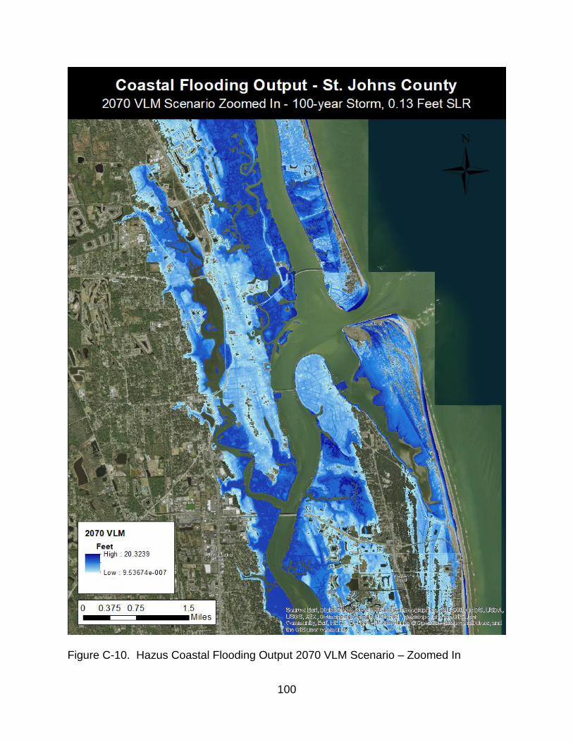
100

Figure C-10. Hazus Coastal Flooding Output 2070 VLM Scenario – Zoomed In

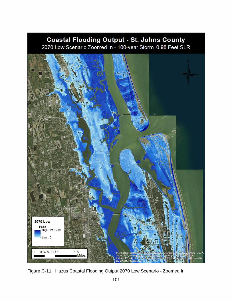
101

Figure C-11. Hazus Coastal Flooding Output 2070 Low Scenario - Zoomed In

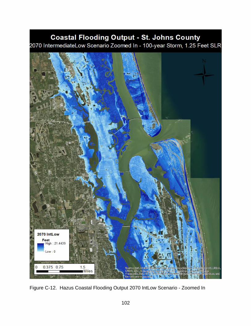
102

Figure C-12. Hazus Coastal Flooding Output 2070 IntLow Scenario - Zoomed In

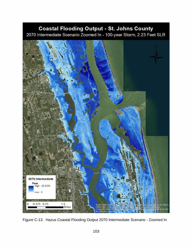
103

Figure C-13. Hazus Coastal Flooding Output 2070 Intermediate Scenario - Zoomed In

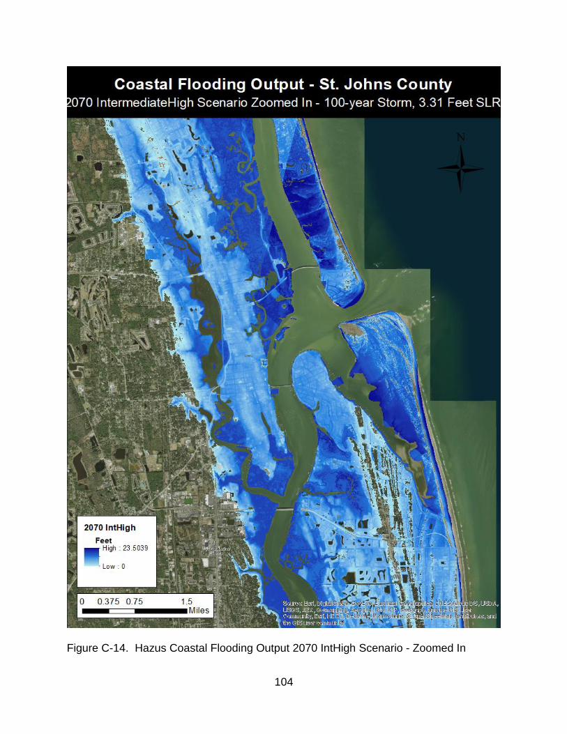
104

Figure C-14. Hazus Coastal Flooding Output 2070 IntHigh Scenario - Zoomed In

105

Figure C-15. Hazus Coastal Flooding Output 2070 High Scenario - Zoomed In

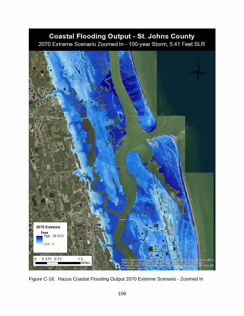
106

Figure C-16. Hazus Coastal Flooding Output 2070 Extreme Scenario - Zoomed In

107

REFERENCES Bureau of Economic Analysis. (2017). Florida. Washington, DC: US Department of

Commerce. Retrieved from https://www.bea.gov/regional/bearfacts/pdf.cfm?fips=12000&areatype=STATE&geotype=3

Carr, M., & Zwick, P. (2016). Florida 2070 Technical Report. Gainesville, FL: University

of Florida GeoPlan Center. Retrieved from http://1000friendsofflorida.org/florida2070/wp-content/uploads/2016/09/florida2070technicalreportfinal.pdf

Chen, C., Beardsley, R., Luettich, R., Westerink, J., Wang, H., & Perrie, W. et al.

(2013). Extratropical storm inundation testbed: Intermodel comparisons in Scituate, Massachusetts. Journal Of Geophysical Research: Oceans, 118(10), 5054-5073. http://dx.doi.org/10.1002/jgrc.20397

Delft University of Technology. (2017). SWAN - Simulating Waves Nearshore. Retrieved

5 January 2018, from http://swanmodel.sourceforge.net/ Department of Homeland Security. (2013). Flood Model - Hazus-MH Technical Manual.

Washington, D.C.: FEMA. Retrieved from https://www.fema.gov/media-library-data/20130726-1820-25045-8292/hzmh2_1_fl_tm.pdf

Federal Emergency Management Agency. (2018). Hazus Overview. fema.gov.

Retrieved 5 January 2018, from https://www.fema.gov/hazus-mh-overview Federal Emergency Management Agency. (2018). RUNUP, Version 2.0. fema.gov.

Retrieved 5 January 2018, from https://www.fema.gov/runup-version-20 Federal Emergency Management Agency. (2018). Wave Height Analysis for Flood

Insurance Studies, Version 4.0. FEMA. Retrieved 5 January 2018, from https://www.fema.gov/wave-height-analysis-flood-insurance-studies-version-40

Florida Bureau of Economic and Business Research. (2015). Florida Estimates of

Population 2015. Gainesville, FL: College of Liberal Arts and Sciences, University of Florida. Retrieved from https://www.bebr.ufl.edu/sites/default/files/Research%20Reports/estimates_2015.pdf

Florida Ocean Alliance. (2013). Florida's Oceans and Coasts: An Economic and Cluster

Analysis. Fort Lauderdale, FL. Retrieved from http://www.floridaoceanalliance.org/wp-content/uploads/2015/08/FLORIDAS_OCEANS_AND_COASTS_AN_ECONOMIC_AND_CLUSTER_ANALYSIS.pdf

108

Frank, K., Volk, M., & Jourdan, D. (2015). Planning for Sea Level Rise in the Matanzas Basin: Opportunities for Adaptation. Gainesville, FL: University of Florida. Retrieved from https://planningmatanzas.files.wordpress.com/2012/06/planning-for-sea-level-rise-in-the-matanzas-basin1.pdf

Frazier, T., Wood, N., & Yarnal, B. (2010). Stakeholder perspectives on land-use

strategies for adapting to climate-change-enhanced coastal hazards: Sarasota, Florida. Applied Geography, 30(4), 506-517. http://dx.doi.org/10.1016/j.apgeog.2010.05.007

Genovese, E., & Green, C. (2014). Assessment of storm surge damage to coastal

settlements in Southeast Florida. Journal Of Risk Research, 18(4), 407-427. http://dx.doi.org/10.1080/13669877.2014.896400

Hall, J.A., S. Gill, J. Obeysekera, W. Sweet, K. Knuuti, and J. Marburger. 2016.

Regional Sea Level Scenarios for Coastal Risk Management: Managing the Uncertainty of Future Sea Level Change and Extreme Water Levels for Department of Defense Coastal Sites Worldwide. Alexandria, VA: U.S. Department of Defense, Strategic Environmental Research and Development Program. 224 pp.

IPCC, 2014. Climate Change 2014: Synthesis Report. Contribution of Working Groups I,

II and III to the Fifth Assessment Report of the Intergovernmental Panel on Climate Change [Core Writing Team, R.K. Pachauri and L.A. Meyer (eds.)]. IPCC, Geneva, Switzerland, 151 pp.

Jones, C., & Griffis, L. (2013). Advances in Hurricane Engineering - Learning from Our

Past - 54. Advanced Estimation of Coastal Storm Surge: Application of SWAN+ADCIRC in Georgia/Northeast Florida Storm Surge Study. American Society of Civil Engineers (ASCE). Retrieved from https://app.knovel.com/hotlink/pdf/id:kt00CCL575/advances-in-hurricane/advanced-estimation-coastal

Karamouz, M., Fereshtehpour, M., Ahmadvand, F., & Zahmatkesh, Z. (2016). Coastal

Flood Damage Estimator: An Alternative to FEMA’s HAZUS Platform. Journal Of Irrigation And Drainage Engineering, 142(6), 04016016. http://dx.doi.org/10.1061/(asce)ir.1943-4774.0001017

Kleinosky, L., Yarnal, B., & Fisher, A. (2006). Vulnerability of Hampton Roads, Virginia

to Storm-Surge Flooding and Sea-Level Rise. Natural Hazards, 40(1), 43-70. http://dx.doi.org/10.1007/s11069-006-0004-z

Kopp, R., Horton, R., Little, C., Mitrovica, J., Oppenheimer, M., & Rasmussen, D. et al.

(2014). Probabilistic 21st and 22nd century sea-level projections at a global network of tide-gauge sites. Earth's Future, 2(8), 383-406. http://dx.doi.org/10.1002/2014ef000239

109

Linhoss, A., Kiker, G., Shirley, M., & Frank, K. (2015). Sea-Level Rise, Inundation, and

Marsh Migration: Simulating Impacts on Developed Lands and Environmental Systems. Journal Of Coastal Research, 299, 36-46. http://dx.doi.org/10.2112/jcoastres-d-13-00215.1

Luettich, R., & Westerink, J. (2017). ADCIRC. adcirc.org. Retrieved 5 January 2018,

from http://adcirc.org/ National Oceanic and Atmospheric Association, (2017). Sea Level Trends.

tidesandcurrents.noaa.gov. Retrieved 11 November 2017, from https://tidesandcurrents.noaa.gov/sltrends/sltrends_station.shtml?stnid=8720218

National Hurricane Center. (2018). SLOSH Model. Sea, Lake, and Overland Surges

from Hurricanes (SLOSH). Retrieved 5 January 2018, from http://www.nhc.noaa.gov/surge/slosh.php

Office of Economic and Demographic Research. (2017). Population and Demographic

Data - Florida Products. edr.state.fl.us. Retrieved 12 January 2018, from http://edr.state.fl.us/Content/population-demographics/data/index-floridaproducts.cfm

Oxford Economics. (2018). The Economic Impact of Out-of-State Visitors in Florida:

2016 Calendar Year Analysis. Tallahassee, FL: Visit Florida. Retrieved from https://www.visitflorida.org/media/30679/florida-visitor-economic-impact-study.pdf

Parris, A., Bromirski, P., Burkett, V., Cayan, D., Culver, M., & Hall, J. et al. (2012).

Global Sea Level Rise Scenarios for the United States National Climate Assessment. Silver Spring, MD: National Oceanic and Atmospheric Administration - Office of Oceanic and Atmospheric Research.

Peng, B. (2015). The Cost-Benefit Analysis of Building Levees to Mitigate the Joint

Effects of Storm Surge and Sea-Level Rise. [electronic resource] A Case Study in City of Miami, Florida. [Gainesville, Fla.] : University of Florida, 2015.

R.S. Means. (2006). Means Square Foot Costs. (27th ed.). Duxbury, Mass. Sebastian, A., Proft, J., Dietrich, J., Du, W., Bedient, P., & Dawson, C. (2014).

Characterizing hurricane storm surge behavior in Galveston Bay using the SWAN+ADCIRC model. Coastal Engineering, 88, 171-181. http://dx.doi.org/10.1016/j.coastaleng.2014.03.002

Stanton, L., M. Davis, and A. Fencl. 2010. Costing Climate Impacts and Adaptation. A

Canadian Study on Coastal Zones. The National Round Table on the Environment and the Economy. Somerville, MA: Stockholm Environmental Institute.

110

Sweet, W., Kopp, R., Weaver, C., Obeysekera, J., Horton, R., Thieler, E., & Zervas, C.

(2017). Global and Regional Sea Level Rise Scenarios for the United States. Silver Spring, MD: National Ocean Service Center for Operational Oceanographic Products and Services - National Oceanic and Atmospheric Administration. Retrieved from https://tidesandcurrents.noaa.gov/publications/techrpt83_Global_and_Regional_SLR_Scenarios_for_the_US_final.pdf

Tol, R. (2002). Estimates of the Damage Costs of Climate Change. Part 1: Benchmark

Estimates. Environmental And Resource Economics, 21(1), 47-73. http://dx.doi.org/10.1023/a:1014500930521

Trigaux, R. (2016). Florida GDP Outpacing U.S. Economic Output Thanks to Strong

Real Estate, Construction Sectors. Tampa Bay Times. Retrieved from http://www.tampabay.com/news/business/florida-gdp-outpacing-us-economic-output-thanks-to-strong-real-estate/2287087

USACE Sea Level Change Curve Calculator. (2017). Climate Preparedness and

Resilience. Retrieved 11 November 2017, from http://www.corpsclimate.us/ccaceslcurves.cfm

Withey, P., Lantz, V., & Ochuodho, T. (2015). Economic costs and impacts of climate-

induced sea-level rise and storm surge in Canadian coastal provinces: a CGE approach. Applied Economics, 48(1), 59-71. http://dx.doi.org/10.1080/00036846.2015.1073843

Xie, D., Zou, Q., & Cannon, J. (2016). Application of SWAN+ADCIRC to tide-surge and

wave simulation in Gulf of Maine during Patriot's Day storm. Water Science And Engineering, 9(1), 33-41. http://dx.doi.org/10.1016/j.wse.2016.02.003

Yohe, G., Neumann, J., Marshall, P., & Ameden, H. (1996). The economic cost of

greenhouse-induced sea-level rise for developed property in the United States. Climatic Change, 32(4), 387-410. http://dx.doi.org/10.1007/bf00140353

Zimmerer, G., Anderson, M., Bellomo, D., Blanton, B., Buckerfield, B., & Collier, K. et al.

(2007). Atlantic Ocean and Gulf of Mexico Coastal Guidelines Update. Denton, TX: FEMA. Retrieved from https://www.fema.gov/media-library-data/1388780453134-c5e577ea3d1da878b40e20b776804736/Atlantic_Ocean_and_Gulf_of_Mexico_Coastal_Guidelines_Update_(Feb_2007).pdf

111

BIOGRAPHICAL SKETCH Adam Carr began his post-secondary education at the University of North

Carolina at Chapel Hill in the Fall of 2009. While there he focused his studies in

environmental science, minoring in geography and entrepreneurship. He was fortunate

enough to participate in a variety of fantastic programs, including study abroad trips to

the US Virgin Islands and Bangkok, Thailand. The experiences he had, especially in

the Thailand program, got Adam interested in urban planning.

After graduating from UNC in 2013, Adam spent two years working for the

National Park Service and the US Forest Service. These positions allowed him to use

some of his skills learned during his undergraduate studies and see different parts of

the country before returning to school.

Adam began his graduate studies at UF in the Fall of 2015 and quickly became

interested in focusing his studies on the application of GIS and spatial analysis in the

context of planning. A Florida native, the issue of sea level rise and impacts from

hurricanes to the built environment was always of interest to him. Focusing his

research on analyzing vulnerability of coastal communities he frequented growing up

and helping these communities understand what steps can be taken moving forward

has been a highlight of his graduate studies at UF.

After completing his studies at UF, Adam hopes to continue using GIS as a tool

to help provide valuable data and analysis to stakeholders involved in any sort of

planning process. This will help generate informed planning decisions that minimize

negative externalities and encourage sustainable, equitable, and resilient outcomes.