Modelica-Driven Power System Modeling, Parameter...
87
Modelica-Driven Power System Modeling, Parameter Identification and Physically-Based Model Aggregation August 12, 2013 JOAN RUSSI ˜ NOL MUSSONS Master’s Degree Project Stockholm, Sweden 2013 XR-EE-ES 2013:011
Transcript of Modelica-Driven Power System Modeling, Parameter...

Modelica-Driven Power System Modeling,
Parameter Identification and
Physically-Based Model Aggregation
August 12, 2013
JOAN RUSSINOL MUSSONS
Master’s Degree Project
Stockholm, Sweden 2013
XR-EE-ES 2013:011


January 2013 to August 2013
Modelica-Driven Power System Modeling, Parameter Identificationand Physically-Based Model Aggregation
— Master Thesis —
Joan Russi
˜
nol Mussons
1
Electrical Power Systems DivisionSchool of Electrical Engineering, KTH Royal Institute of Technology, Sweden
Supervisor and ExaminerProf. Dr.-Ing. Luigi Vanfretti
KTH Stockholm
SupervisorTetiana Bogodorova
KTH Stockholm
Stockholm, August 12, 2013


Abstract
Historically, dynamic modeling and simulation in power systems community is performed us-ing di↵erent and mostly incompatible softwares. Even though there have been great e↵ortsin the development of the Common Information Model (CIM) for power system applications,there are still many challenges for power system dynamic modeling without any ambiguity.Therefore, exists a need to develop unambiguous models which can be reused in di↵erentsimulation environments and become universally compatible. Moreover, there is a need for aformal mathematical language that can allow for dynamic model exchange without ambiguity.Such language could compliment the CIM standard and e↵orts.
In recent research, the Modelica language has been proposed as the definitive solution tothese challenges due to the flexibility and mathematical formalism that the language providesfor dynamic model representation. Modelica is a relatively new object-oriented language spe-cially born in order to meet the model development requirements. The Modelica language isan equation based language with a clear focus on model reutilization.
In this project the Modelica modeling will play a major role, in addition the reader will findsome practical advice on developing power system component models in Modelica.
In addition, this thesis discusses power system model parameter identification and aggrega-tion. Using synthetic measurement data derived from simulations, the parameters of a modelare identified.
This thesis illustrates the application of Modelica for power system modeling and simulation,as well as the ability for unambiguous model exchange. It also shows how Modelica and FMItechnologies can be combined and utilize for power system simulation.
Finally, this thesis shows examples of application of the RaPId Toolbox for power systemparameter identification and physical-based model aggregation.
iii


Acknowledgments
First of all, I would like to thank Prof.Dr.-Ing. Luigi Vanfretti for giving me this opportu-nity as his Master Thesis student and to Juan Antonio Martınez Velasco for providing me hiscontact. In addition, I would like to thank very specially Tetiana Bodogorova for her guidance.
To continue, I would like to thank all the people who helped me and supported me duringthe duration of this project. In particular, I would like to thank specially all the members ofthe KTH SmarTS Lab.
In addition, I would like to mention and thank again Prof.Dr.-Ing. Luigi Vanfretti and FarhanMahmood for providing me the Simulink models which were used to obtain the synthetic mea-surement data. The original model of the feeder used for load model aggregation in Chapter5 was provided by Dr. Alan Collinson of SP Energy Networks and implemented in SimPow-erSystems/Simulink by Farhan Maahmood and Dr. Luigi Vanfretti of KTH SmarTS Lab.
During this project I consider that I made friends who were of great support and I would liketo mention them as well (in alphabetical order): Naveed Ahmad, Achour Amazouz, ViktorAppelgreen, Maxime Baudette, Rokibul Hasan, Farhan Mahmood, Dr. Rafael Segundo andmany more people who made my stay at KTH a pleasure.
Finally, I would like to thank my family for their support and for giving me their valuableadvice, as well as all the friends I made in Kista (The Kista People) and my Spanish friends.
This research project was supported by the iTesla Collaborative R&D project funded by theEuropean Commission.
Joan Russinol MussonsAugust 12, 2013
v


Contents
Notation ix
List of Figures xi
1. Introduction 11.1. Background . . . . . . . . . . . . . . . . . . . . . . . . . . . . . . . . . . . . . 11.2. Problem Definition . . . . . . . . . . . . . . . . . . . . . . . . . . . . . . . . . 21.3. Objectives . . . . . . . . . . . . . . . . . . . . . . . . . . . . . . . . . . . . . . 21.4. Contributions . . . . . . . . . . . . . . . . . . . . . . . . . . . . . . . . . . . . 31.5. Overview of the Report . . . . . . . . . . . . . . . . . . . . . . . . . . . . . . 3
2. Modelica, Equation-Based Modeling and Simulation 52.1. Introduction to Modelica . . . . . . . . . . . . . . . . . . . . . . . . . . . . . . 5
2.1.1. Re-usability . . . . . . . . . . . . . . . . . . . . . . . . . . . . . . . . . 52.1.2. Modeling and Simulation Modelica Software Environments . . . . . . 6
2.2. Modelica Basics . . . . . . . . . . . . . . . . . . . . . . . . . . . . . . . . . . . 62.3. Simulation Parameters . . . . . . . . . . . . . . . . . . . . . . . . . . . . . . . 8
3. Implementing Power System Models in Modelica 113.1. Introduction . . . . . . . . . . . . . . . . . . . . . . . . . . . . . . . . . . . . . 113.2. Connectors . . . . . . . . . . . . . . . . . . . . . . . . . . . . . . . . . . . . . 123.3. Power System Modeling Guidelines . . . . . . . . . . . . . . . . . . . . . . . . 133.4. List of Symbols . . . . . . . . . . . . . . . . . . . . . . . . . . . . . . . . . . . 153.5. Generators . . . . . . . . . . . . . . . . . . . . . . . . . . . . . . . . . . . . . 15
3.5.1. Second Order . . . . . . . . . . . . . . . . . . . . . . . . . . . . . . . . 153.5.2. Third Order . . . . . . . . . . . . . . . . . . . . . . . . . . . . . . . . . 153.5.3. Component to Network Interface . . . . . . . . . . . . . . . . . . . . . 16
3.6. Generator Controls . . . . . . . . . . . . . . . . . . . . . . . . . . . . . . . . . 163.6.1. Turbine Governor . . . . . . . . . . . . . . . . . . . . . . . . . . . . . 163.6.2. Automatic Voltage Regulator . . . . . . . . . . . . . . . . . . . . . . . 16
3.7. Loads . . . . . . . . . . . . . . . . . . . . . . . . . . . . . . . . . . . . . . . . 173.7.1. Constant P and Q . . . . . . . . . . . . . . . . . . . . . . . . . . . . . 173.7.2. Voltage Dependent Load . . . . . . . . . . . . . . . . . . . . . . . . . . 173.7.3. ZIP Load . . . . . . . . . . . . . . . . . . . . . . . . . . . . . . . . . . 183.7.4. Frequency Dependent Load . . . . . . . . . . . . . . . . . . . . . . . . 183.7.5. Exponential Recovery Load . . . . . . . . . . . . . . . . . . . . . . . . 183.7.6. Jimma’s Load . . . . . . . . . . . . . . . . . . . . . . . . . . . . . . . . 19
vii

Contents
3.7.7. Mixed Load . . . . . . . . . . . . . . . . . . . . . . . . . . . . . . . . . 193.7.8. Order I Induction Machine . . . . . . . . . . . . . . . . . . . . . . . . 19
3.8. Photovoltaic Models . . . . . . . . . . . . . . . . . . . . . . . . . . . . . . . . 203.8.1. PSAT Photovoltaic Generators . . . . . . . . . . . . . . . . . . . . . . 203.8.2. Power Factory Photovoltaic Model . . . . . . . . . . . . . . . . . . . . 20
3.9. Software-to-Software Validation . . . . . . . . . . . . . . . . . . . . . . . . . . 223.9.1. Generator Validation . . . . . . . . . . . . . . . . . . . . . . . . . . . . 243.9.2. Solar Photovoltaics, TG and AVR . . . . . . . . . . . . . . . . . . . . 243.9.3. Load Validation . . . . . . . . . . . . . . . . . . . . . . . . . . . . . . 24
4. System Identification and Parameter Estimation 294.1. Introduction . . . . . . . . . . . . . . . . . . . . . . . . . . . . . . . . . . . . . 294.2. General Optimization Algorithms . . . . . . . . . . . . . . . . . . . . . . . . . 30
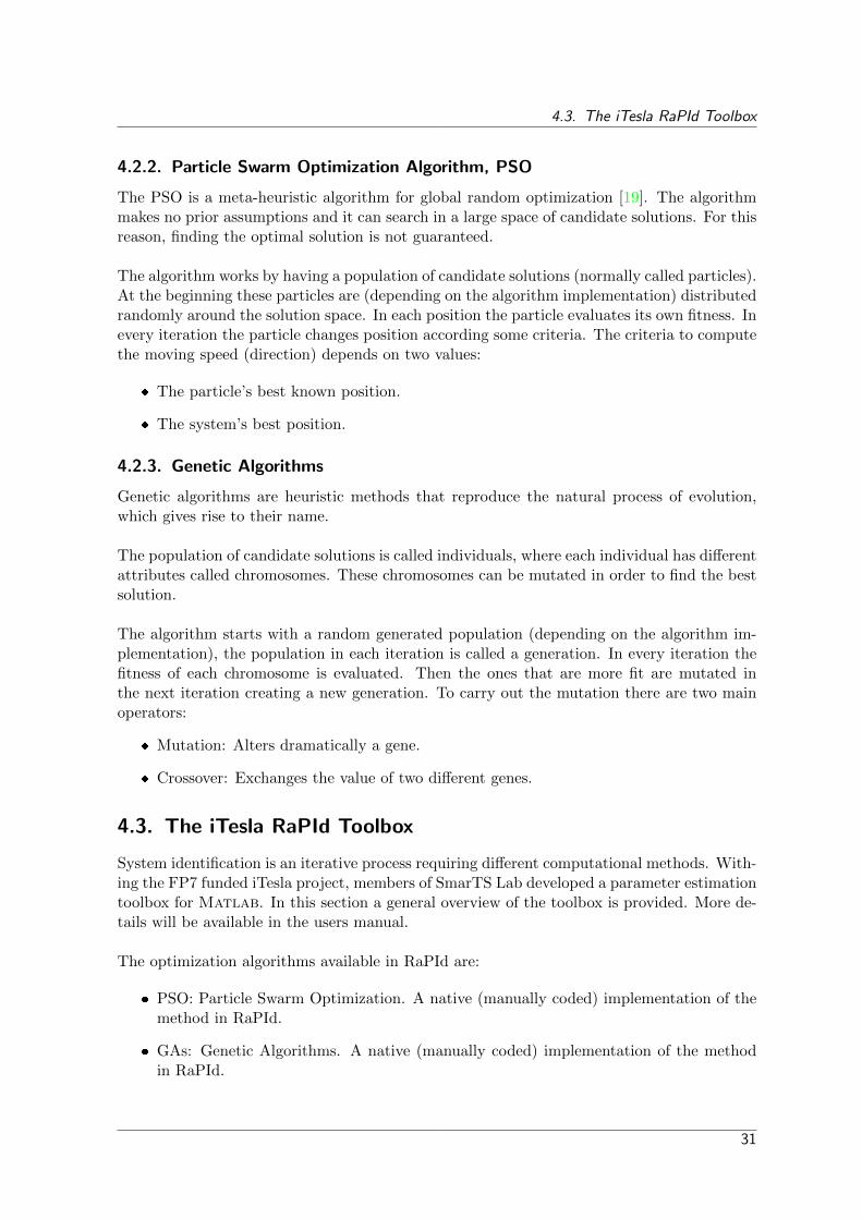
4.2.1. Gradient Descent Method . . . . . . . . . . . . . . . . . . . . . . . . . 304.2.2. Particle Swarm Optimization Algorithm, PSO . . . . . . . . . . . . . 314.2.3. Genetic Algorithms . . . . . . . . . . . . . . . . . . . . . . . . . . . . . 31
4.3. The iTesla RaPId Toolbox . . . . . . . . . . . . . . . . . . . . . . . . . . . . . 31
5. Power System Model Identification 375.1. Introduction . . . . . . . . . . . . . . . . . . . . . . . . . . . . . . . . . . . . . 375.2. Parameter Estimation Case Generator . . . . . . . . . . . . . . . . . . . . . . 38
5.2.1. Methodology for Estimating Generator Parameters . . . . . . . . . . . 405.2.2. Results . . . . . . . . . . . . . . . . . . . . . . . . . . . . . . . . . . . 42
5.3. Load Aggregation . . . . . . . . . . . . . . . . . . . . . . . . . . . . . . . . . . 455.3.1. Load Aggregate Model Identification Results . . . . . . . . . . . . . . 48
5.4. Photovoltaic Panel Parameter Estimation Case . . . . . . . . . . . . . . . . . 52
6. Discussion 576.1. Modelica . . . . . . . . . . . . . . . . . . . . . . . . . . . . . . . . . . . . . . . 57
6.1.1. Models . . . . . . . . . . . . . . . . . . . . . . . . . . . . . . . . . . . 576.1.2. Model Exchange . . . . . . . . . . . . . . . . . . . . . . . . . . . . . . 57
6.2. System Identification . . . . . . . . . . . . . . . . . . . . . . . . . . . . . . . . 586.2.1. RaPId Toolbox . . . . . . . . . . . . . . . . . . . . . . . . . . . . . . . 586.2.2. Thesis Results . . . . . . . . . . . . . . . . . . . . . . . . . . . . . . . 58
7. Conclusion and Future Work 617.1. Conclusions . . . . . . . . . . . . . . . . . . . . . . . . . . . . . . . . . . . . . 617.2. Future Work . . . . . . . . . . . . . . . . . . . . . . . . . . . . . . . . . . . . 61
Bibliography 63
A. Appendix 65A.1. Software-to-Software Model Validation Results . . . . . . . . . . . . . . . . . 65
viii

Notation
AC Alternating Current
AVR Automatic Voltage Regulator
DC Direct Current
EMTP Electro-Magnetic Transient Programs
FMI Functional Mock-up Interface
FMU Functional Mock-up Unit
GUI Graphic User Interface
KTH Kungliga Tekniska Hogskolan
OSS Open Source Software
P Active Power
PF Power Factory
PMU Phasor Measurement Unit
PSAT Power System Analysis Toolbox
PV Photovoltaic
Q Reactive Power
SPS SimPowerSystems
TG Turbine Governor
ZIP Constant Impedance, Current, Power
ix


List of Figures
2.1. Example power system model in Modelica . . . . . . . . . . . . . . . . . . . . 72.2. A Modelica model displayed in text, icon and diagram view (shown using Wol-
fram System Modeler) . . . . . . . . . . . . . . . . . . . . . . . . . . . . . . . 82.3. Simulation options in System Modeler and Dymola . . . . . . . . . . . . . . . 9
3.1. Connection between two electrical power system models from [1] . . . . . . . 133.2. Electrical connector from [1] in OpenModelica . . . . . . . . . . . . . . . . . . 133.3. Icon of the third order generator implemented . . . . . . . . . . . . . . . . . . 143.4. Example on how to describe parameters . . . . . . . . . . . . . . . . . . . . . 143.5. Turbine governor block diagram [2] . . . . . . . . . . . . . . . . . . . . . . . 163.6. Automatic voltage regulator block diagram [2] . . . . . . . . . . . . . . . . . 173.7. Comparison between the model in Power Factory and Modelica . . . . . . . 213.8. Model of the PV cell . . . . . . . . . . . . . . . . . . . . . . . . . . . . . . . . 213.9. ZIP-Jimma load software-to-software validation . . . . . . . . . . . . . . . . . 243.10. PSAT and Modelica models used to validate the generator models . . . . . . 253.11. PSAT and Modelica models used to validate the Solar Photovolatics, TG and
AVR models . . . . . . . . . . . . . . . . . . . . . . . . . . . . . . . . . . . . . 253.12. PSAT and Modelica models used to validate the loads models . . . . . . . . . 26
4.1. A system with inputs, outputs and perturbations . . . . . . . . . . . . . . . . 294.2. System identification illustration . . . . . . . . . . . . . . . . . . . . . . . . . 304.3. Modelica model to be converted to FMU . . . . . . . . . . . . . . . . . . . . . 334.4. Generating an FMU from Dymola . . . . . . . . . . . . . . . . . . . . . . . . 344.5. General diagram of the main internal computation loop used in RaPId . . . . 354.6. Main Graphical User Interface (GUI) of the iTesla raPId Toolbox . . . . . . . 36
5.1. Schematic of the testing model structure . . . . . . . . . . . . . . . . . . . . 375.2. Comparison between machines with di↵erent inertias . . . . . . . . . . . . . 395.3. Comparison between machines with di↵erent damping coe�cients . . . . . . 395.4. Comparison between machines with di↵erent direct axis time constant . . . . 405.5. Simulink model of the testing system . . . . . . . . . . . . . . . . . . . . . . 405.6. Simulink model with the FMU of the Modelica model . . . . . . . . . . . . . 415.7. Methodology used for the identification process . . . . . . . . . . . . . . . . . 425.8. Comparison between the reference (Simulink) and the identified (Modelica)
model responses for the torque perturbation . . . . . . . . . . . . . . . . . . . 435.9. Comparison between the reference (Simulink) and the identified (Modelica)
model responses for the field voltage perturbation . . . . . . . . . . . . . . . . 44
xi

List of Figures
5.10. Validation of the identified generator model parameters for the torque pertur-bation . . . . . . . . . . . . . . . . . . . . . . . . . . . . . . . . . . . . . . . . 44
5.11. Validation of the identified generator model parameters for the field voltageperturbation . . . . . . . . . . . . . . . . . . . . . . . . . . . . . . . . . . . . 45
5.12. Scottish Power distribution grid corresponding to the modeled load [3] . . . . 465.13. Modelica model in the identification process . . . . . . . . . . . . . . . . . . . 465.14. RaPId Simulink model for the load aggregation case . . . . . . . . . . . . . . 475.15. Exponential recovery aggregate load model results . . . . . . . . . . . . . . . 485.16. Voltage dependent aggregate load model results . . . . . . . . . . . . . . . . . 495.17. Frequency dependent aggregate load model Results . . . . . . . . . . . . . . . 505.18. ZIP Results . . . . . . . . . . . . . . . . . . . . . . . . . . . . . . . . . . . . . 525.19. Modelica model in the identification process. . . . . . . . . . . . . . . . . . . 535.20. RaPId Simulink model for the PV panel parameter identification . . . . . . . 535.21. Panel parameter identification statistical analysis . . . . . . . . . . . . . . . . 555.22. Panel parameter identification simulation results against reference data . . . 56
A.1. Second order synchronous machine software-to-software validation . . . . . . 65A.2. Third order synchronous machine software-to-software validation . . . . . . . 66A.3. Automatic voltage regulator software-to-software validation . . . . . . . . . . 66A.4. Turbine governor software-to-software validation . . . . . . . . . . . . . . . . 67A.5. Constant P,Q load software-to-software validation . . . . . . . . . . . . . . . . 67A.6. ZIP load software-to-software validation . . . . . . . . . . . . . . . . . . . . . 68A.7. ZIP-Jimma load software-to-software validation . . . . . . . . . . . . . . . . . 68A.8. Voltage dependent load software-to-software validation . . . . . . . . . . . . . 69A.9. Exponential recovery load software-to-software validation . . . . . . . . . . . 69A.10.Frequency dependent load software-to-software validation . . . . . . . . . . . 70A.11.Mixed load software-to-software validation . . . . . . . . . . . . . . . . . . . . 70A.12.Induction machine software-to-software validation . . . . . . . . . . . . . . . . 71A.13.Constant P Q generator software-to-software validation . . . . . . . . . . . . 71A.14.Constant P V generator software-to-software validation . . . . . . . . . . . . 72A.15.KTH PV model software-to-software validation (Irradiation change) . . . . . 72A.16.KTH PV model software-to-software validation (Temperature change) . . . . 73
xii

1 Introduction
1.1. Background
Power systems are very complex and they expose a high variety of dynamic phenomena. Forthese reasons, di↵erent modeling and simulation approaches have been proposed as the coreof power systems simulation softwares, in order to meet di↵erent simulations requirements [4].
Simulation models are increasingly being used in problem solving and to aid in decision-making [5]. Many tools in order to create power systems simulation models exist, howeverthey are incompatible. The reasons why they are not compatible can be categorized as follows[4]:
Data format incompatibility.
Di↵erent dynamics models.
Di↵erent modeling approaches and predefined models.
To overcome these di�culties, recent research suggests the use of formal mathematical mod-eling languages, in particular, Modelica [4]. Modelica is a standardized language which isobject-oriented and equation-based, specially born in order to create models of physical com-ponents. Modelica o↵ers several advantages against other tools, for example:
Straightforward and open modification of models.
A common standard modeling language.
Unambiguous model exchange between Modelica simulation environments.
In addition, modeling is only one part of the problem, the other part is to match the modelsbehavior with the actual behavior recorded from the field measurements. This is known asmodel validation and calibration. To perform model validation, system identification tech-niques must be applied. These techniques allow the model response to match the systemmeasured response by using a combination of tools to correct the model by, for example,optimally changing model parameters.
1

1. Introduction
1.2. Problem Definition
Modeling and simulation are becoming more important since engineers need to analyze com-plex systems, often using components from di↵erent domains [6]. This is becoming increas-ingly important in power systems, for example in the context of PMU-based wide-area control.Modelica o↵ers the possibility of multi-domain modeling, however, a suitable power systemsModelica library is needed to perform cyber-physical power system studies involving di↵erentdomains, as in the wide-area control example.
Several attempts for power systems modeling using the Modelica language have been madein recent years [7]. Despite these attempts, those libraries became proprietary and closed formodifications. Other Open Source Software (OSS) libraries have not been updated to supportthe latest Modelica language standard, which would require users to make substantial andoften di�cult changes to utilize them. In essence, there was no up to date OSS Modelicalibrary in order to simulate power systems.
Additionally, having good mathematical models is not enough. To be useful, the models mustmatch the actual behavior as measured in the field, by for instance tunning their parameters.This model to reality fitting can be done using di↵erent techniques.
The problems this thesis focuses on are:
Contribute to the development of Open Source power systems Modelica models to beincluded in a library being developed within the FP7 iTesla project.
Propose methods for parameter estimation and model aggregation.
Provide examples of the developed methods applied to power systems.
1.3. Objectives
In order to deal with the problems listed above the following objectives were set:
Perform a literature review.
Learn the Modelica language and model implementation specifics.
Develop power system component models in Modelica.
Develop some power system component Modelica modeling guidelines.
Perform parameter estimation and aggregation on power system models.
Provide illustrative examples of the power of Modelica and its ability for model ex-change.
These ambitious objectives were set to illustrate the benefits of using Modelica for powersystems and will be the foundation for future work in the area.
2
1.4. Contributions
1.4. Contributions
This thesis is part of the European Project iTesla, concretely work-packages 3.3 and 3.4. Allthe information that can be found in this report is a direct contribution towards it.
In addition, the Modelica models implemented in this thesis contribute as well to the Power-Systems Open-Source Modelica library, which is being developed in collaboration with “GrupoAIA (Spain)”, “RTE (France)” and “KTH SmarTS Lab”, with Prof.Dr.-Ing. Luigi Vanfrettias work-package leader.
This thesis was also used as an example of the use of a new toolbox for system identifica-tion called RaPId. The toolbox was developed in KTH SmarTS Lab by Achour Amazouzand Prof.Dr.-Ing. Luigi Vanfretti, funded through the European Commission within the FP7iTesla project.
1.5. Overview of the Report
The report is divided in two main parts:
1. Modelica for power systems.
2. System identification for parameter estimation and physically-based power system modelaggregation.
The first part is the basis for all the thesis. It includes Chapter 2 and Chapter 3. In Chapter2 an introduction to Modelica can be found, whereas, Chapter 3 contains the practical appli-cation of Modelica for power system modeling.
The second half consists in system identification for parameter estimation and physical-basedpower system model aggregation. In Chapter 4 there is an introduction to the system iden-tification techniques used and in Chapter 5 the practical applications of these techniques topower systems can be found.
Finally, at the end of the report discussions and conclusions are provided.
3


2 Modelica, Equation-Based Modeling and Simulation
2.1. Introduction to Modelica
Modelica is a non-proprietary standardized language, thus is not protected by trademark,patent or copyright. Modelica is an object-oriented and declarative language. It has beendeveloped in order to conveniently model dynamic behavior of complex physical systems, forexample, mechanical, hydraulic, electric and other domains.
The fact what distinguishes Modelica from other languages is that it is object-oriented equa-tion based language, that means, that each model is described itself by equations. The use ofequations allows a greater flexibility since they do not prescribe a certain data flow [8].The four most important features of Modelica are [9]:
Modelica is based on equations instead of assignment statements. This permits anacausal modeling that gives better reuse of classes since equations do not specify a cer-tain data flow direction.
Modelica has multi-domain modeling capability, meaning that model components cor-responding to physical objects from several di↵erent domains can be described andconnected.
Modelica is an object-oriented language with a general class concept that unifies classesand general sub-typing into a single language construct. This facilitates reuse of com-ponents and evolution of models.
Modelica has a strong software component model, with constructs for creating and con-necting components. Thus, the language is ideally suited as an architectural descriptionlanguage for complex physical systems, and to some extent for software systems.
2.1.1. Re-usability
A model is reusable in Modelica because it is modeled independently of the environmentwhere it will be used. This is achieved by including in the definition of each component its
5

2. Modelica, Equation-Based Modeling and Simulation
equations using only local variables and connectors. Thus, there is no connection between acomponent and the rest of the system, except from the connector.
2.1.2. Modeling and Simulation Modelica Software Environments
As it was stated before, Modelica is a non-proprietary language so it can be used for free byanyone. For this reason, a wide range of softwares based on Modelica is now available (seeTable 2.1).
Table 2.1.: Modelica simulation enviroments
Proprietary simulation environments Open source simulation environments
CyModelica Jmodelica.orgDymola Modelicac
MOSILAB OpenModelicaSimulationX SimForge
LMS Imagine.Lab AMESimMapleSim
OPTIMICA StudioMworks
Wolfram System Modeler
All the softwares are based on Modelica language, the biggest di↵erence among them is the in-terface they use. This variety allows the engineer to choose the tool more suitable to him/her.In order to pursue this thesis, System Modeler and Dymola were used.
2.2. Modelica Basics
Modelica is a transparent programming language which allows the user to create very complexmodels.
Like in other programming languages, in Modelica there exist the type parameter and thetype variable. One parameter is a type which contains a value that is set at the start of thesimulation and will remain constant during it. On the other hand, a variable is a type whichcontains a value that changes withing time. In Modelica, defining a parameter or a variableis straightforward, as shown in Fig.2.1.
The propierty that most characterizes Modelica is the way it allows the user to introduceequations that are always accurate. For that purpose, the programmer must state when theequation section starts. On the contrary, if the programmer wants to execute a routine in aspecific order, an algorithm should be used. See Fig.2.1. These two concepts are summarizedwith the following simple definitions:
Equation: mathematical statement, example : F = ma.
6

2.2. Modelica Basics
Algorithm: sequence of calculations that leads to a result.
In Fig.2.1 a basic model can be found. Fig.2.1 shows how parameters, variables and equationscan be used to design a power system component model.
Figure 2.1.: Example power system model in Modelica
Further details on the Modelica language can be found in [9].
When using Modelica based tools there exist three types of model views:
1. The text view.
Is where the code is written. All the graphical modifications will have an impact on it.
2. The icon view.
Is where the graphical representation of the model will be designed. In essence, allowsto define the model’s graphical appearance.
3. The diagram view.
Is where the user can drag and drop previously made models, the models will appearas an instance with the appearance created in the icon view.
To exemplify these three views, please observe Fig.2.2 which shows the same model displayedin di↵erent views.
7

2. Modelica, Equation-Based Modeling and Simulation
Figure 2.2.: A Modelica model displayed in text, icon and diagram view (shown using Wol-fram System Modeler)
2.3. Simulation Parameters
In Modelica programming environments the simulation solvers are decoupled from the model.This makes easier the exchange of models. Di↵erent softwares provide di↵erent solvers andoptions.
The basic characteristics that will change the outputs of the simulations are the solver used,the integration time step and the tolerance. The engineer can choose between several kindsof solvers. In general, there are two distinct types of solvers:
Solvers with automatic integration step: the step is adaptive, i.e. it changes accordingto the dynamics of the system, this allows for fast simulation time.
Solvers with constant integration step: during the simulation the time step remains
8

2.3. Simulation Parameters
constant.
When simulating with a constant time step, choosing a large step will make the simulationtake less time, but at the same time it will be less accurate, on the other hand, if the inte-gration step is too small the simulation will be large.
In Fig.2.3 the simulation options of System Modeler and Dymola are shown.
Solver
Tolerance
Interval length (Step)
Figure 2.3.: Simulation options in System Modeler and Dymola
9

3 Implementing Power System Models in Modelica
3.1. Introduction
In this chapter a detailed explanation of the power system models implemented in Modelicais given. The models presented are based from another software used as reference, namelyPSAT. PSAT is a power systems toolbox for Matlab developed by Federico Milano. Furtherinformation can be found in the PSAT manual [2].
Implementing the same models from PSAT in Modelica is a challenging task. The way PSATworks is completely di↵erent from Modelica. The steps to achieve a successful implementationare the followings:
Understand the conceptual background of the model.
Read the PSAT documentation of the model.
Identify the main equations that define the dynamic behavior of the model.
Locate the initialization equations.
Write the model in Modelica.
Perform a software-to-software validation of the Modelica model against the PSATmodel.
Validation is a key issue when implementing models. The procedure followed in order tovalidate the models is detailed at the end of this chapter. The software-to-software validationwill consist in a comparison of the behavior when using the same test system in PSAT andModelica. The results from the experiments performed can be found in Appendix A.
When comparing both softwares two observations were made:
Modelica simulates faster than PSAT and gives more options for solving the system ofequations (additional solvers).
Implementing a model in Modelica requires less time than in PSAT. In addition, thetraining required to implement a model in Modelica is lower than for PSAT.
Finally, outstanding challenges of this part of the project were:
11

3. Implementing Power System Models in Modelica
The aim of the study is to match the actual dynamic behavior of the system, the mod-els developed are “phasor-time domain” or “positive sequence” models that disregardcertain system dynamics.
No power flow tool was developed to be integrated along Modelica, all the power flowsolutions were taken from PSAT.
3.2. Connectors
In order to interface di↵erent component models, Modelica has a predefined class calledconnector. This class ensures that the models can be reusable and independent from eachother. It can host two types of variables:
Standard connector (without any prefix): This type of connector ensures that the mag-nitude and the sign of the variable are the same.
Flow connector (flow prefix): This type of connector is based in the principle of sumequal to zero.
Notice that in Modelica the flow connection has a sign convention. It is defined as positivewhen the flow enters the connector and it is defined as negative when the flow exits the con-nector. An illustration of such type of connector is shown in Fig.3.1.
It is very important to understand that the models have to be defined according to theconnectors. During this thesis two kinds of connectors have been used:
Connectors for real signals.
Connectors for electrical signals.
To connect real signals, for example, the torque of a generator, the standard connector Realdefined in Modelica has been used. In this case, this connector already exists in the ModelicaStandard Library. This kind of connector is based in the principle of equality. For equality itis understood that when two components are connected their value is the same (magnitudeand sign).
On the other hand, for the electrical connections an specific connector has been used, thisconnector was first develop in [1],[10]. The basic structure of the connector is shown in Fig.3.2.
It is important to notice that the electrical connector is defined in terms of real part andimaginary part of the voltage and current phasors. This means that despite the electricalmagnitudes are phasors, the library does not use complex values, instead it uses real valuesdefined in Cartesian coordinates.
12

3.3. Power System Modeling Guidelines
Figure 3.1.: Connection between two electrical power system models from [1]
Figure 3.2.: Electrical connector from [1] in OpenModelica
3.3. Power System Modeling Guidelines
As it was stated before, creating models in Modelica is not very complex. But in order tocreate models that can be reused, some criteria must be followed:
The final model should be one simple block. In the case that the model was created byparts and then they were just connected, the programmer must aggregate them in oneblock and icon.
The parameters that the user can modify must be stated on the top-layer block of themodel. In models made up from di↵erent blocks, the user must not have to look insidethem in order to change any parameter.
In addition, the developer should define the model parameters with a default value inthe top-layer of the model.
The programmer must use labels to identify the blocks and their corresponding connec-tors, as shown in Fig.3.3.
All the parameters must be described using strings, so the user knows what they are,as shown in Fig.3.4.
Use the attribute public/protected. Public: visible and changeable by anything. Pro-tected: cannot be changed by a modifier.
Import constants from Modelica.Constants.
There are three ways to initialize the model; through auxiliary parameters or throughinitial equations or algorithms. Each of them have their own advantages and disad-vantages. For example, when using an auxiliary parameter it is possible to check the
13

3. Implementing Power System Models in Modelica
correctness of the value, but the code becomes more di�cult to understand. The oppo-site happens when using initial equations or algorithms. Finally, when using auxiliaryparameters to initialize the model it is recommended to label them with a string mes-sage.
Figure 3.3.: Icon of the third order generator implemented
Figure 3.4.: Example on how to describe parameters
14
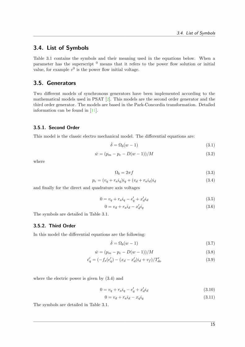
3.4. List of Symbols
3.4. List of Symbols
Table 3.1 contains the symbols and their meaning used in the equations below. When aparameter has the superscript 0 means that it refers to the power flow solution or initialvalue, for example v0 is the power flow initial voltage.
3.5. Generators
Two di↵erent models of synchronous generators have been implemented according to themathematical models used in PSAT [2]. This models are the second order generator and thethird order generator. The models are based in the Park-Concordia transformation. Detailedinformation can be found in [11].
3.5.1. Second Order
This model is the classic electro mechanical model. The di↵erential equations are:
� = ⌦b
(w � 1) (3.1)
w = (pm
� pe
�D(w � 1))/M (3.2)
where
⌦b
= 2⇡f (3.3)
pe
= (vq
+ ra
iq
)iq
+ (vd
+ ra
id
)id
(3.4)
and finally for the direct and quadrature axis voltages
0 = vq
+ ra
iq
� e0q
+ x0d
id
(3.5)
0 = vd
+ ra
id
� x0d
iq
(3.6)
The symbols are detailed in Table 3.1.
3.5.2. Third Order
In this model the di↵erential equations are the following:
� = ⌦b
(w � 1) (3.7)
w = (pm
� pe
�D(w � 1))/M (3.8)
e0q
= (�fs
(e0q
)� (xd
� x0d
)id
+ vf
)/T 0do
(3.9)
where the electric power is given by (3.4) and
0 = vq
+ ra
iq
� e0q
+ x0d
id
(3.10)
0 = vd
+ ra
id
� xq
iq
(3.11)
The symbols are detailed in Table 3.1.
15

3. Implementing Power System Models in Modelica
3.5.3. Component to Network Interface
The interface with the electrical connector is carried out using the Park’s transformation:
ir
ii
�= �
sin(�) cos(�)�cos(�) sin(�)
� id
iq
�(3.12)
vr
vi
�=
sin(�) cos(�)�cos(�) sin(�)
� vd
vq
�(3.13)
where ir
and ii
correspond to the real part and the imaginary part of the connector current,and v
r
,vi
correspond to the real and imaginary part of the connector voltage.
The symbols are detailed in Table 3.1.
3.6. Generator Controls
Two control blocks for the generators were implemented. An Automatic Voltage Regulator(AVR) and a Turbine Governor (TG). These models are based on the PSAT AVR TypeII andTG TypeIII models that can be found in [2].
The symbols are detailed in Table 3.1.
3.6.1. Turbine Governor
The turbine governor implemented in Modelica can be seen in Fig.3.5.
Figure 3.5.: Turbine governor block diagram [2]
Fig.3.5 model has three input signals the actual rotor speed (w), the reference rotor speed(w
ref
) and the power flow initial mechanical power (p0m
). The output of the block is themechanical power that must be applied to the generator (p
m
).
3.6.2. Automatic Voltage Regulator
The automatic voltage regulator is based on the exciter type III from PSAT where it has beensimplified. It can be seen in figure 3.6.
16

3.7. Loads
Figure 3.6.: Automatic voltage regulator block diagram [2]
Fig.3.6 model has three input signals: the actual voltage (v), the reference voltage (vref
) andthe power flow initial field voltage (v0
f
). The output of the block is the field voltage (vf
) thatmust be applied to the generator.
3.7. Loads
The general equation which all the loads follow is given by
S = P + jQ = V I⇤ = (vr
+ jvi
)(ir
� jii
) (3.14)
Discerning between real part and imaginary part results in
P = vr
⇤ ir
+ vi
ii
(3.15)
Q = vi
⇤ ir
� vr
ii
(3.16)
In the following subsections di↵erent types of loads will be presented, the di↵erence betweenthem will be the way P and Q are defined and calculated. The symbols are detailed in Table3.1.
3.7.1. Constant P and Q
Constant P and Q load is the simplest type of load. During simulation the value of the activepower and the reactive power will remain the same.
P = constant (3.17)
Q = constant (3.18)
3.7.2. Voltage Dependent Load
Voltage dependent loads are loads for which the value of the active power and the reactivepower depends on the bus voltage in which they are connected to.
P = P 0(v/v0)↵p (3.19)
Q = Q0(v/v0)↵q (3.20)
17

3. Implementing Power System Models in Modelica
3.7.3. ZIP Load
A ZIP load has three components: the constant impedance(Z), the constant current(I) andthe constant power(P) injections [12]. The model that has been implemented is the following:
P = p0z
(v/v0)2 + p0i
(v/v0) + p0p
(3.21)
Q = q0z
(v/v0)2 + q0i
(v/v0) + q0p
(3.22)
3.7.4. Frequency Dependent Load
Based on PSAT [2], by di↵erentiating and filtering the phase angle of the bus the frequencydeviation, �w, is approximated and the frequency dependency of the loads is introduced asfollows:
x = ��w/TF
(3.23)
0 = x+1
2⇡fn
TF
(✓ � ✓0)��w (3.24)
P = P 0(v/v0)↵p(1 +�w)�p (3.25)
Q = Q0(v/v0)↵q(1 +�w)�q (3.26)
3.7.5. Exponential Recovery Load
The model implemented is exactly the same proposed in PSAT [2]. The values of P and Qrecovers from a voltage change according to an exponential curve.
For the active power:
xp
= �xp
/Tp
+ ps
� pt
(3.27)
p = xp
/Tp
+ pt
(3.28)
ps
= P 0(v/v0)↵s (3.29)
pt
= P 0(v/v0)↵t (3.30)
For the reactive power:
xq
= �xq
/Tq
+ qs
� qt
(3.31)
q = xq
/Tq
+ qt
(3.32)
qs
= Q0(v/v0)�s (3.33)
qt
= Q0(v/v0)�t (3.34)
18
3.7. Loads
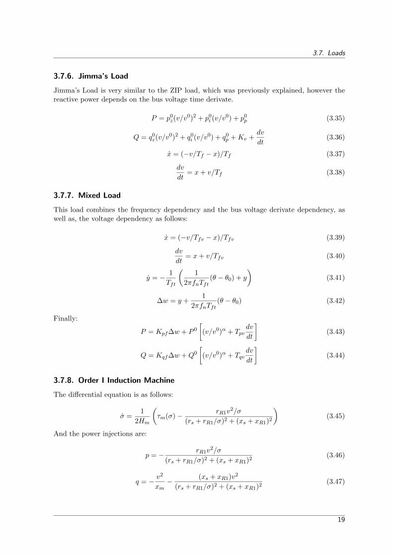
3.7.6. Jimma’s Load
Jimma’s Load is very similar to the ZIP load, which was previously explained, however thereactive power depends on the bus voltage time derivate.
P = p0z
(v/v0)2 + p0i
(v/v0) + p0p
(3.35)
Q = q0z
(v/v0)2 + q0i
(v/v0) + q0p
+Kv
+dv
dt(3.36)
x = (�v/Tf
� x)/Tf
(3.37)
dv
dt= x+ v/T
f
(3.38)
3.7.7. Mixed Load
This load combines the frequency dependency and the bus voltage derivate dependency, aswell as, the voltage dependency as follows:
x = (�v/Tfv
� x)/Tfv
(3.39)
dv
dt= x+ v/T
fv
(3.40)
y = � 1
Tft
✓1
2⇡fn
Tft
(✓ � ✓0) + y
◆(3.41)
�w = y +1
2⇡fn
Tft
(✓ � ✓0) (3.42)
Finally:
P = Kpf
�w + P 0
(v/v0)↵ + T
pv
dv
dt
�(3.43)
Q = Kqf
�w +Q0
(v/v0)↵ + T
qv
dv
dt
�(3.44)
3.7.8. Order I Induction Machine
The di↵erential equation is as follows:
� =1
2Hm
✓⌧m
(�)� rR1v
2/�
(rs
+ rR1/�)2 + (x
s
+ xR1)2
◆(3.45)
And the power injections are:
p = � rR1v
2/�
(rs
+ rR1/�)2 + (x
s
+ xR1)2
(3.46)
q = � v2
xm
� (xs
+ xR1)v2
(rs
+ rR1/�)2 + (x
s
+ xR1)2
(3.47)
19
3. Implementing Power System Models in Modelica
3.8. Photovoltaic Models
First, very simple photovoltaic generators from PSAT [2] were implemented (constant PQ,constant PV), but theses models were not detailed enough. So it was decided to implementa more detailed PV model based on previous work [13].
3.8.1. PSAT Photovoltaic Generators
The implemented models were constant PQ and constant PV. The models were designedin PSAT in order to perform transient and voltage stability analysis. For this reason, onlysimplified controllers driving a controllable source were modeled.
3.8.2. Power Factory Photovoltaic Model
This model was provided by Farhan Mahmood and the reference simulation model was de-veloped in Power Factory. The complete documentation can be found in [13].
In comparison with the models from PSAT this model includes several additional featuressuch as PV panel’s dynamics, which implies the dependency on irradiation and temperature.
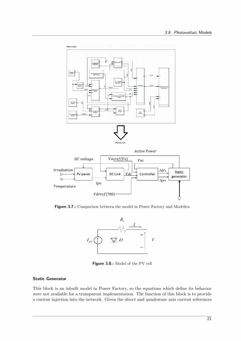
The model is composed by several sub-blocks: PV panel (composed by several PV cells), DClink, Controller and a Static Generator.
The model implemented in Modelica is shown and compared with the reference Power Factorymodel in Fig.3.7
PV Cell
The PV cell was modeled as a current source in parallel with a diode and in series with aresistance as shown in Fig.3.8.
DC Link
The DC link is modeled as a capacitor, where the variation of the DC voltage multiplied bythe capacitance provides the current.
Controller
The controller is aimed to keep the AC voltage and DC voltage at the same reference value.In addition, it calculates the reference direct axis current and the quadrature axis current.
20
3.8. Photovoltaic Models
Figure 3.7.: Comparison between the model in Power Factory and Modelica
Figure 3.8.: Model of the PV cell
Static Generator
This block is an inbuilt model in Power Factory, so the equations which define its behaviorwere not available for a transparent implementation. The function of this block is to providea current injection into the network. Given the direct and quadrature axis current references
21

3. Implementing Power System Models in Modelica
the model regulate the actual injected currents. In addition, it includes the interface with thegrid (the electrical connector). To sum up, the main two functions of this block are:
Interface with the grid.
Control the currents.
To control the current the following equations were assumed
Id
= (Idref
� Id
)/Td
(3.48)
Iq
= (Iqref
� Iq
)/Tq
(3.49)
To interface with the grid the following equations were assumed
Ir
= (Id
⇤ cos(✓)� Iq
⇤ sin(✓)) (3.50)
Ii
= (Id
⇤ sin(✓) + Iq
⇤ cos(✓)) (3.51)
Initialization
In order to initialize the previous equations the following system of algebraic equations wasto be solved.
Vr
= V0 ⇤ cos(✓0) (3.52)
Vi
= V0 ⇤ sin(✓0) (3.53)
A = Vi
⇤ cos(✓0)� Vr
⇤ sin(✓0) (3.54)
B = Vr
⇤ cos(✓0) + Vi
⇤ sin(✓0) (3.55)
Id
= (P0 ⇤B +Q0 ⇤A)/(A2 +B2) (3.56)
Iq
= (P0 ⇤A�Q0 ⇤B)/(A2 +B2) (3.57)
3.9. Software-to-Software Validation
As the models implemented in Modelica language are based in other software tools, it hassense that the validation is done by comparing the output results of both softwares when theinput system is the same.
Software-to-software validation was carried out by designing di↵erent test scenarios. Thisprocedure required to compare outputs of two systems given the same input (perturbationson the reference signals) and the same system structure (parameters). Ideally, a correct modelwill provide a one to one match between the corresponding output signals.
The following numerical experiments were created.
For the synchronous machines:
22

3.9. Software-to-Software Validation
Vref
pulse of 0.0005 at t = [2-2.1].
Vref
oscillation 0.001sin(0.2) at t=[0-5].
Pm
pulse of 0.005 at t = [7-7.1].
Pm
oscillation 0.001sin(0.2) at t = [5-10].
Fault at t=[10-10.1] with fault impedance parameters R=20 and X=1.
Line opening at t = [14-14.1].
For the induction machine, solar photovoltaics, TG and the AVR:
Fault at t=[3-3.1] with fault impedance parameters R=20 and X=1.
Line opening at t = [8-8.1].
For the loads:
Vref
pulse of 0.0005 at t = [2-2.1].
Vref
oscillation 0.001sin(0.2) at t=[0-5].
Pm
pulse of 0.005 at t = [7-7.1].
Pm
oscillation 0.001sin(0.2) at t = [5-10].
For the detailed solar PV model:
Irradiation change from 1000 W/m2 to 500 W/m2 and back to 1000 W/m2 at t=[0.3-0.7].
Temperature change from 25 �C to 40 �C and back to 25 �C at t=[0.3-0.7].
The validation results can be found in Appendix A.
In order to provide an example of the results please see Fig.3.9 .
Discussion: The software-to-software validation proved the Modelica capability for powersystem modeling. Achieving more accurate results than PSAT, as it is shown in Fig.3.9.Modelica computational power allowed a reduction of the integration step without increasingthe computation time, thus providing smoother and more accurate results. To design correctsoftware-to-software experiments the nature of the validated component must be taken intoaccount.
23

3. Implementing Power System Models in Modelica
0 5 100.437
0.4371
0.4371
0.4372
0.4372
0.4373
G Gen
erat
or-T
3
Time(s.)
PSATModelica
0 5 100.9998
1
1.0002
1.0004
1.0006
1.0008
1.001
Z
Time(s.)
PSATModelica
0 5 100.991
0.992
0.993
0.994
0.995
0.996
V3
Time(s.)
PSATModelica
0 5 101.7175
1.718
1.7185
1.719
1.7195
1.72
v f
Time(s.)
PSATModelica
0 5 100.079
0.0795
0.08
0.0805
0.081
0.0815
0.082
Pm
Time(s.)
PSATModelica
0 5 100.07
0.072
0.074
0.076
0.078
0.08
0.082
0.084
P3
Time(s.)
PSATModelica
0 5 100.0599
0.06
0.06
0.0601
Q3
Time(s.)
PSATModelica
Figure 3.9.: ZIP-Jimma load software-to-software validation
3.9.1. Generator Validation
For validating the generator the models used are shown in Fig.3.10. The PSAT model andthe PSAT perturbation are shown together with the corresponding model in Modelica.
The validation system in Fig.3.10 is composed by four buses. The fault is located in busnumber four, which is connected by a power line to bus number two. This structure waschosen in order to avoid to locate the fault directly on the load side, thus being less severe.
3.9.2. Solar Photovoltaics, TG and AVR
For validating the Solar Photovoltaics, Induction Machine, TG and AVR the models used areshown in Fig.3.11.
The validation system in Fig.3.10 is composed by four buses. The fault is located in busnumber four, which is connected by a power line to bus number two. This structure waschosen in order to avoid to locate the fault directly on the load side, thus being less severe.
3.9.3. Load Validation
The models used for validating the load models are shown in Fig.3.12.
The validation system in Fig.3.12 is composed by three buses. This test system is simplerbecause for testing the load models the fault was not required.
24

3.9. Software-to-Software Validation
PSAT Model PSAT Perturbation
GENERATOR VALIDATION SCHEME
Modelica
Figure 3.10.: PSAT and Modelica models used to validate the generator models
PSAT Model
SOLAR & INDUCTION MACHINE VALIDATION SCHEME
Modelica
TG & AVR VALIDATION SCHEME
PSAT Model Modelica
Figure 3.11.: PSAT and Modelica models used to validate the Solar Photovolatics, TG andAVR models
25
Luigiv

3. Implementing Power System Models in Modelica
PSAT Model PSAT Perturbation
Modelica
LOAD VALIDATION SCHEME
Figure 3.12.: PSAT and Modelica models used to validate the loads models
26

3.9. Software-to-Software Validation
Table 3.1.: List of Symbols
Symbol Meaning
� Rotor angle index⌦b
Grid angular’s speedw Rotor angular speedpm
Mechanical powerpe
Electrical powerD Damping coe�cientM Mechanical starting timevd
Direct axis voltagevq
Quadrature axis voltageid
Direct axis currentiq
Quadrature axis currentra
Armature resistancexd
Direct axis reactancex0d
Direct axis transient reactancexq
Quadrature axis reactanceeq
Quadrature axis transient voltageT 0do
Transient time constantR Turbine governor dropP Active powerQ Reactive powerT Time constantK Gainvf
Field voltage↵p
Active power voltage exponent↵q
Reactive power voltage exponent�p
Active power frequency coe�cient�q
Reactive power frequency coe�cientTp
Active power time constantTq
Reactive power time constant↵s
Static active power exponent↵t
Dynamic active power exponent�s
Static reactive power exponent�t
Dynamic reactive power exponent✓ Bus voltage angle
Hm
Inertia constantrs
Stator resistancexs
Stator reactancerR1 1st order cage rotor resistance
xR1 1st order cage rotor reactance� Slip⌧ Torque
27


4 System Identification and Parameter Estimation
4.1. Introduction
System identification links mathematical models to real life observations. Particularly, sys-tem identification consist in building models of real life dynamic systems from observationsof their actual behavior [14].
A system is formed by a set of elements which interact in an integrated structure. Thereare several kinds of systems: mechanical, electrical, natural, etc. The interest on systems isto study their behavior and to determine how they will interact when subjected to externalperturbations.
Systems can be excited by input signals and perturbations as depicted in Fig.4.1. The dif-ference between input signals and perturbations its how they are originated. Inputs signalsare signals which are under the user control, whereas, perturbations are signal which cannotbe controlled and appear spontaneously. Finally, the output signals are the response of thesystem to the stimuli.
A car is an example of a system, see Fig.4.2. If we consider a car as the system, the inputsignals would be the position of the throttle and the breaking pedal. As it can be noticed,those two signals are fully controlled by the driver. The perturbations might be the roadinclination, the wind speed, the tra�c, etc., and the output would be the speed of the vehicle.
Figure 4.1.: A system with inputs, outputs and perturbations
Once the system is observed and its boundaries are clearly defined it is possible to considermodels. A model is the representation of a system. Human kind create models of everythingthey want to study. Mathematical models may consist of a set of equations which relate theoutput of the system with the inputs and the perturbations.
29
4. System Identification and Parameter Estimation
A simple mathematical model can consist of a simple transfer function, but nowadays thesystems that are being modeled are very complex and the process of creating models is be-coming more challenging and important. One key factor for this massive development ofmodels is the increase of computing capacity, which allows us to use these models to performcomputations in a very e�cient manner.
System identification consist in matching the real behavior with the model. For example,estimating the parameters of the model.
Figure 4.2.: System identification illustration
4.2. General Optimization Algorithms
Notice that in order to perform the system identification and the parameter estimation proce-dure some general optimization algorithms were used. The function of these general optimiza-tion algorithm was to proportionate the best matching between the reality and the model,these algorithm have been used in order to search the parameters which minimize the errorbetween the measured data and the simulated model.
The methods explained below are very well-known techniques so only a basic description ofthem is given. Further information can be found in the cited literature [15], [16], [17], [18].
4.2.1. Gradient Descent Method
The gradient descent method is a first order optimization method. The objective is to findthe local minimum of a a function based on its gradient. The principle is to take steps pro-portional to the negative of the gradient.
This method is simple but slow because it needs to evaluate the gradient at each iteration.Moreover, this method easily gets trapped in local minimuma. To avoid the local minimuma,new methods have been developed. The method works for any number of dimensions.
30
4.3. The iTesla RaPId Toolbox
4.2.2. Particle Swarm Optimization Algorithm, PSO
The PSO is a meta-heuristic algorithm for global random optimization [19]. The algorithmmakes no prior assumptions and it can search in a large space of candidate solutions. For thisreason, finding the optimal solution is not guaranteed.
The algorithm works by having a population of candidate solutions (normally called particles).At the beginning these particles are (depending on the algorithm implementation) distributedrandomly around the solution space. In each position the particle evaluates its own fitness. Inevery iteration the particle changes position according some criteria. The criteria to computethe moving speed (direction) depends on two values:
The particle’s best known position.
The system’s best position.
4.2.3. Genetic Algorithms
Genetic algorithms are heuristic methods that reproduce the natural process of evolution,which gives rise to their name.
The population of candidate solutions is called individuals, where each individual has di↵erentattributes called chromosomes. These chromosomes can be mutated in order to find the bestsolution.
The algorithm starts with a random generated population (depending on the algorithm im-plementation), the population in each iteration is called a generation. In every iteration thefitness of each chromosome is evaluated. Then the ones that are more fit are mutated inthe next iteration creating a new generation. To carry out the mutation there are two mainoperators:
Mutation: Alters dramatically a gene.
Crossover: Exchanges the value of two di↵erent genes.
4.3. The iTesla RaPId Toolbox
System identification is an iterative process requiring di↵erent computational methods. With-ing the FP7 funded iTesla project, members of SmarTS Lab developed a parameter estimationtoolbox for Matlab. In this section a general overview of the toolbox is provided. More de-tails will be available in the users manual.
The optimization algorithms available in RaPId are:
PSO: Particle Swarm Optimization. A native (manually coded) implementation of themethod in RaPId.
GAs: Genetic Algorithms. A native (manually coded) implementation of the methodin RaPId.
31
4. System Identification and Parameter Estimation
NAIVE: A naive method. A native (manually coded) implementation of a simplegradient-based method in RaPId.
CG: Conjugate Gradient. This method uses the Matlab function Fminun for opti-mization.
NM: Nelder-Mead method. This method uses the Matlab function Pminsearch foroptimization.
COMBI: Combination. This method allows the combination usage of two methodssequentially, after a determined number of iterations. The idea is to allow the user toutilize a PSO or GA method to find the region of the global minimum, and then agradient-based method to iterate towards the final solution.
PSOext: PSO external. This method uses the Global Optimization Toolbox functionsfrom Matlab.
GAext. GA external. This method uses the Global Optimization Toolbox functionsfrom Matlab.
Next, the methodology used in order to identify the system will be explained, from creatingthe model to parameter identification. The main steps in this process are the following:
1. Collect measurement data (which will be used in order to identify the system).
2. Create the power system model in Modelica.
3. Compile an FMU from the Modelica model.
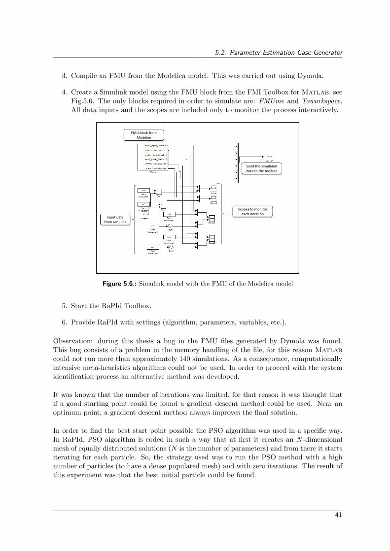
4. Create a Simulink model using the FMU block from the FMI Toolbox for Matlab [20].
5. Start the RaPId Toolbox.
6. Input the settings required by RaPId for the particular case (algorithm, parameters,variables, etc.).
7. Simulate and collect the results.
8. Evaluate the results.
Collect measurement data
As it was previously explained system identification requires reference data. The referencedata will be compared with the simulations one in order to obtain the fitness and modify theparameters. In the ideal case, the data should be measured data, but for the purpose of thisthesis the data used as reference was generated from a simulation of the model in Simulink,see Fig.5.5.
Observe that, if the data used comes from measurements it will have noise. The noise in thesignals makes the identification process harder and, in order to achieve good results, somesignal processing should be performed.
32
4.3. The iTesla RaPId Toolbox
Create the power system model in Modelica
The assumed model to be identified should be created in Modelica. This step can be per-formed according to di↵erent criteria, including the type of perturbations to be applied tothe system and how the user wants to exploit the model using Simulink.
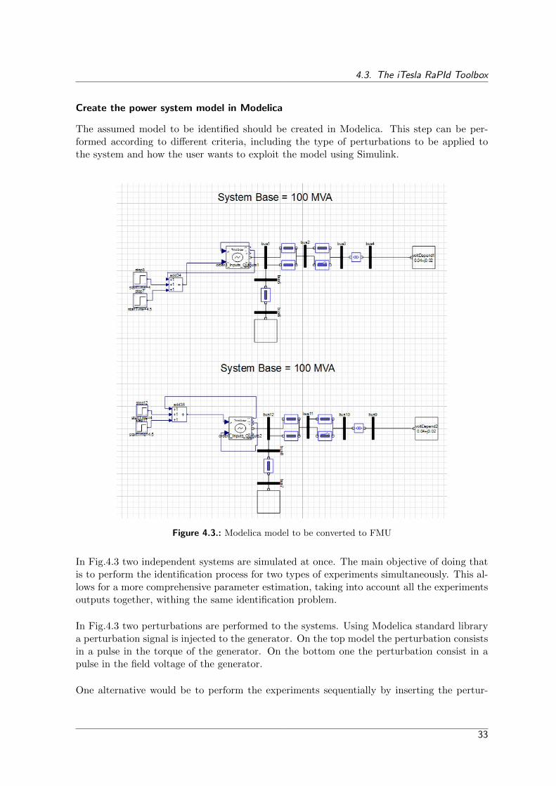
Figure 4.3.: Modelica model to be converted to FMU
In Fig.4.3 two independent systems are simulated at once. The main objective of doing thatis to perform the identification process for two types of experiments simultaneously. This al-lows for a more comprehensive parameter estimation, taking into account all the experimentsoutputs together, withing the same identification problem.
In Fig.4.3 two perturbations are performed to the systems. Using Modelica standard librarya perturbation signal is injected to the generator. On the top model the perturbation consistsin a pulse in the torque of the generator. On the bottom one the perturbation consist in apulse in the field voltage of the generator.
One alternative would be to perform the experiments sequentially by inserting the pertur-
33

4. System Identification and Parameter Estimation
bations withing the same simulation, but by placing them in two dedicated experiments weavoid any possible interference in between them.
Compile an FMU from the Modelica model.
The iTesla RaPId Toolbox uses the Modelica models as the mathematical models of realsystems via the FMI Toolbox for Matlab.A Functional Mock-up Unit (FMU) is generated by using Dymola which is compliant withthe FMI standard (Functional Mock-up interface). The FMI is a tool independent standardfor the exchange of dynamic models and for Co-Simulation [21].
The FMI standard provides a common standardized interface for model exchange betweendi↵erent software tools for di↵erent applications [22], realizing this interface through an FMU.
When generating a FMU file two types of FMU can be chosen:
FMU for Model Exchange: generates lime C-Code or object code containing the dynamicsystem model in the form of an input/output block.
FMU for Co-Simulation: is similar to the FMU for Model Exchange, with the di↵erencethat it includes the solvers together with the models.
In order to be able to simulate the models using the solvers provided in Matlab Simulink,the FMU for model exchange was chosen.
To generate FMU files the FMI functionalities in Dymola were used. Other Modelica pro-gramming and simulation environments started to provide this functionality which will be astandard feature in the future [23]. This option in Dymola can be found in the simulationmenu as shown in Fig.4.4.
Figure 4.4.: Generating an FMU from Dymola
34

4.3. The iTesla RaPId Toolbox
Create a Simulink model using the FMI Toolbox for Matlab
The Simulink model needs to utilize an FMU Block for model exchange from the FMI Toolboxfor Matlab. The FMU needs to be loaded and configured in this block. After simulation, itredirects the results from the simulation to the toolbox, serving as a link in between Simulinkand RaPId.
An example of this Simulink model can be found in Fig.5.6. More information can be foundin the next chapter.
iTesla RaPId Toolbox
The RaPId toolbox plays a major role as a tool for this thesis to perform parameter identifica-tion. It simulates the model contained in the FMU, calculates the fitness of the results againstthe reference data and, according an optimization algorithm, it modifies the parameters ofthe FMU model. A simplified diagram is shown in Fig.4.5. More extensive explanation canbe found in the documentation of the toolbox, developed withing the FP7 iTesla project byKTH SmarTS Lab.
Measured Data
FMU model
Fitness criteria
satisfied?
Simulate
Algorithm
Change Parameters
End
Yes No
Signal Processing
Figure 4.5.: General diagram of the main internal computation loop used in RaPId
In Fig.4.6 the main user interface of RaPId is presented. On the left hand side, the di↵erentsettings and options can be provided and, on the right hand side, the algorithm and resultscan be instantiated. On the bottom the user must provide output (mandatory) and input(optional) measured data.
35

4. System Identification and Parameter Estimation
Algorithm Selection
Results and Plots
Simulink
Provide the output measurement data
Provide the measurement data
Options and Settings
Figure 4.6.: Main Graphical User Interface (GUI) of the iTesla raPId Toolbox
The RaPId Toolbox can be as well used thought a textual interface.
36
5 Power System Model Identification
5.1. Introduction
In this chapter the procedure for power system model parameter identification and physically-based model aggregation is presented. In addition, the methodology for validating the powersystem models and the parameters identified will be discussed.
The reference measurement data, which will be used in order to identify the systems, was ob-tained from the Simulink models developed using SimPowerSystems Matlab library. Thesemodels have a higher bandwidth and more detailed representation typically used in Electro-Magnetic Transient Programs (EMTP). Thus, the SimPowerSystems Simulink models areconsidered as the reference.
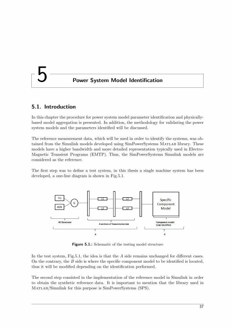
The first step was to define a test system, in this thesis a single machine system has beendeveloped, a one-line diagram is shown in Fig.5.1.
Figure 5.1.: Schematic of the testing model structure
In the test system, Fig.5.1, the idea is that the A side remains unchanged for di↵erent cases.On the contrary, the B side is where the specific component model to be identified is located,thus it will be modified depending on the identification performed.
The second step consisted in the implementation of the reference model in Simulink in orderto obtain the synthetic reference data. It is important to mention that the library used inMatlab/Simulink for this purpose is SimPowerSystems (SPS).
37

5. Power System Model Identification
In this thesis three system identification and parameter estimation cases are presented:
1. Generator parameter estimation: All the component parameters in the test system areknown with exception of the generators model parameters. Once the parameters of thegenerator are identified, they will be used for the load aggregation.
2. Load aggregation: In this case, an unknown load will be placed in the system. Theidentification will consist in matching the behavior of the load to di↵erent load models.
3. PV panel parameter estimation. This case is used to illustrate how specific unknown oruncertain parameters of a component model can be identified given su�cient knowledgeof other model parameters.
5.2. Parameter Estimation Case Generator
Generator models in SPS and Modelica are not identical. The Modelica model has a simpli-fied representation of the generator’s dynamics (a 3rd order model) while the SPS modul usesa very detailed EMTP-type representation. The goal here is to identify the parameters of asimplified dynamic model of a generator that can match the electro-mechanical dynamics ofthe reference model. To accomplish this goal a known load has been located in the componentmodel side (B) and two perturbations are applied to the system. These perturbation are infact the experiments designed for this identification case.
The first perturbation is a pulse of duration 0.5 seconds of 1 % the nominal torque in theshaft of the generator. The second perturbation is a pulse of duration 0.5 seconds of 1 %the nominal field voltage of the machine. Using the results from these two perturbations, theparameters of the machine are estimated.
The most relevant parameters, which rule the electro-mechanical dynamic behavior of thesystem, depend on the perturbation. Thus, the design of these experiments is relevant for theidentification procedure.
Perturbations in the torque will primarily excite mechanical dynamics. Hence, for torqueperturbations the inertia of the machine is important. Inertia regulates the amplitude andthe frequency of the oscillations. The damping coe�cient will have similar e↵ects with higherimpact on the amplitude of the oscillations.
Fig.5.2 shows simulations results from two systems, the only di↵erence between both is theinertia of the machine. It can be observed that the machine with lower inertia oscillatesfaster and with a larger amplitude. Fig.5.3 shows simulation results from two systems, theonly di↵erence between both is the damping coe�cient of the machine, it can be observedthat when the coe�cient is larger the system will be damped more.
On the other hand, when tunning the system with respect to field voltage perturbations,the direct axis time constant has an important impact on the output powers. This happensbecause this constant has a large impact on machine voltage dynamics. This impact can be
38

5.2. Parameter Estimation Case Generator
0 5 10 150.9998
0.9998
0.9999
0.9999
1
1
1.0001
1.0001
Wge
n
Time(s.)
Low InertiaBig Inertia
Figure 5.2.: Comparison between machines with di↵erent inertias
0 5 10 150.9999
0.9999
1
1
1
1
1
1.0001
1.0001
Wge
n
Time(s.)
D=0D=4
Figure 5.3.: Comparison between machines with di↵erent damping coe�cients
observed in Fig.5.4.
39

5. Power System Model Identification
0 5 10 150.0204
0.0205
0.0206
0.0207
0.0208
0.0209
0.021
0.0211
Qge
n
Time(s.)
Low Direct Axis Time ConstantHigh Direct Axis Time Constant
Figure 5.4.: Comparison between machines with di↵erent direct axis time constant
5.2.1. Methodology for Estimating Generator Parameters
The generator model used includes 7 parameters and 4 output quantities are measured foreach of the experiments (in total 8 outputs must match). This is not a trivial problemand a good approach to formulate the identification problem is needed because the space ofpossible solutions is immense (7th dimensional space). Following the general process detailedin Chapter 4, the method used here is stated as follows:
1. Collect measurement data: this is carried out with Simulink using the test system inFig.5.5. The data collected was the voltage (magnitude), the rotor speed and, thepowers (the machine active power and reactive power).
Figure 5.5.: Simulink model of the testing system
2. Create the power system model in Modelica, see Fig.4.3 (contains both experimentsin order to include them in the identification process simultaneously). The Modelicamodel requires a power flow solution, in this case the results of the power flow wereobtained from PSAT.
40
5.2. Parameter Estimation Case Generator
3. Compile an FMU from the Modelica model. This was carried out using Dymola.
4. Create a Simulink model using the FMU block from the FMI Toolbox for Matlab, seeFig.5.6. The only blocks required in order to simulate are: FMUme and Toworkspace.All data inputs and the scopes are included only to monitor the process interactively.
Send the simulated data to the toolbox
FMU block from Modelon
Scopes to monitor each iteration
Input data from simulink
Figure 5.6.: Simulink model with the FMU of the Modelica model
5. Start the RaPId Toolbox.
6. Provide RaPId with settings (algorithm, parameters, variables, etc.).
Observation: during this thesis a bug in the FMU files generated by Dymola was found.This bug consists of a problem in the memory handling of the file, for this reason Matlab
could not run more than approximately 140 simulations. As a consequence, computationallyintensive meta-heuristics algorithms could not be used. In order to proceed with the systemidentification process an alternative method was developed.
It was known that the number of iterations was limited, for that reason it was thought thatif a good starting point could be found a gradient descent method could be used. Near anoptimum point, a gradient descent method always improves the final solution.
In order to find the best start point possible the PSO algorithm was used in a specific way.In RaPId, PSO algorithm is coded in such a way that at first it creates an N -dimensionalmesh of equally distributed solutions (N is the number of parameters) and from there it startsiterating for each particle. So, the strategy used was to run the PSO method with a highnumber of particles (to have a dense populated mesh) and with zero iterations. The result ofthis experiment was that the best initial particle could be found.
41

5. Power System Model Identification
In order to have a 7-dimension uniform mesh at least 128 (27) particles in RaPId were required.
Once the initial particle was found, the NM method [24] (a simplex optimization method) wasused. The methodology is synthesized in Fig.5.7.
Methodology:
1. Run PSO natively implemented in RaPId with 1 iteration and the maximum number of particles. Why? 2. This particle is a good starting point for a gradient descent method, a better solution can be found iteratively with this method. Note: This methodology must be run several times changing the weights of the fitness function to have different solutions.
The PSO coded in RaPId initializes the particles in the n-dimensional space solution in a regular way (not random).
N dimensions for N parameters
The minimum number of particles is 2N. The result from the PSO will be the particle with best fitness.
The NM method is suggested and executed until the FMI Toolbox crashes, when it crashes last value found can be obtained and the method can be
re-runned using these last values as starting point.
Figure 5.7.: Methodology used for the identification process
5.2.2. Results
The numerical results of the generator parameter estimation process are shown in Table 5.1
Table 5.1.: Generator parameter estimation results
Parameter Value
Armature resistance (Ra
) 0.0010156Direct axis reactance (X
d
) 4.2924Direct axis transient reactance (X 0
d
) 1.37Direct axis transient time constant (T 0
d
) 2.6156Quadrature axis reactance (X
q
) 5.3994Inertia coe�cient (M) 14.9005Damping ratio (D) 0.0088415
Graphical results are presented in Fig.5.8 and Fig.5.9.
42

5.2. Parameter Estimation Case Generator
Discussion: In Table 5.1 the values of the identified parameters are shown. The numericalvalue for all the parameters are inside the normal range for a generator. That means, thevalues of the parameters are in the standard range and there are no anomalies like negativesparameters. In Fig.5.8 and Fig.5.9 are shown the graphical comparison between the simu-lations in SPS and Modelica. In the graphical comparison the matching is not 100% butthe error is acceptable. In Fig.5.8 all the outputs plots match well except for the reactivepower, in Fig. 5.9 all the outputs plots match well except for the voltage magnitude. Thesedi↵erences are due to the di↵erent nature of the models in SPS (EMTP) and Modelica.
In order to validate the results of identification, the simulations in both SPS/Simulink andModelica were repeated using perturbations two-times larger than the original experimentsused for identification. The results are shown in Fig.5.10 and Fig.5.11.
0 1 2 3 4 5 6 7 8 9 100.999
0.9995
1
1.0005
Vge
n
Time(s.)
ModelicaSimulink
0 1 2 3 4 5 6 7 8 9 100.39
0.4
0.41
Pge
n
Time(s.)
ModelicaSimulink
0 1 2 3 4 5 6 7 8 9 100.202
0.204
Qge
n
Time(s.)
ModelicaSimulink
0 1 2 3 4 5 6 7 8 9 100.9998
0.9999
1
1.0001
Wge
n
Time(s.)
ModelicaSimulink
0 1 2 3 4 5 6 7 8 9 100.4
0.405Pm
Time(s.)
ModelicaSimulink
Figure 5.8.: Comparison between the reference (Simulink) and the identified (Modelica)model responses for the torque perturbation
43

5. Power System Model Identification
0 1 2 3 4 5 6 7 8 9 100.999
1
1.001
Vge
n
Time(s.)
ModelicaSimulink
0 1 2 3 4 5 6 7 8 9 100.395
0.4
0.405
0.41
Pge
n
Time(s.)
ModelicaSimulink
0 1 2 3 4 5 6 7 8 9 10
0.202
0.204
0.206
Qge
n
Time(s.)
ModelicaSimulink
0 1 2 3 4 5 6 7 8 9 1011111
Wge
n
Time(s.)
ModelicaSimulink
0 1 2 3 4 5 6 7 8 9 101
2
3
Vf
Time(s.)
ModelicaSimulink
Figure 5.9.: Comparison between the reference (Simulink) and the identified (Modelica)model responses for the field voltage perturbation
0 1 2 3 4 5 6 7 8 9 100.999
0.9995
1
1.0005
Vge
n
Time(s.)
ModelicaSimulink
0 1 2 3 4 5 6 7 8 9 100.39
0.4
0.41
Pge
n
Time(s.)
ModelicaSimulink
0 1 2 3 4 5 6 7 8 9 100.2
0.202
0.204
0.206
Qge
n
Time(s.)
ModelicaSimulink
0 1 2 3 4 5 6 7 8 9 100.9998
1
1.0002
Wge
n
Time(s.)
ModelicaSimulink
0 1 2 3 4 5 6 7 8 9 100.4
0.405Pm
Time(s.)
ModelicaSimulink
Figure 5.10.: Validation of the identified generator model parameters for the torque pertur-bation
44
5.3. Load Aggregation
0 1 2 3 4 5 6 7 8 9 100.999
1
1.001
1.002
Vge
n
Time(s.)
ModelicaSimulink
0 1 2 3 4 5 6 7 8 9 100.395
0.4
0.405
0.41
Pge
n
Time(s.)
ModelicaSimulink
0 1 2 3 4 5 6 7 8 9 10
0.202
0.204
0.206
Qge
n
Time(s.)
ModelicaSimulink
0 1 2 3 4 5 6 7 8 9 1011111
Wge
n
Time(s.)
ModelicaSimulink
0 1 2 3 4 5 6 7 8 9 101
2
3
Vf
Time(s.)
ModelicaSimulink
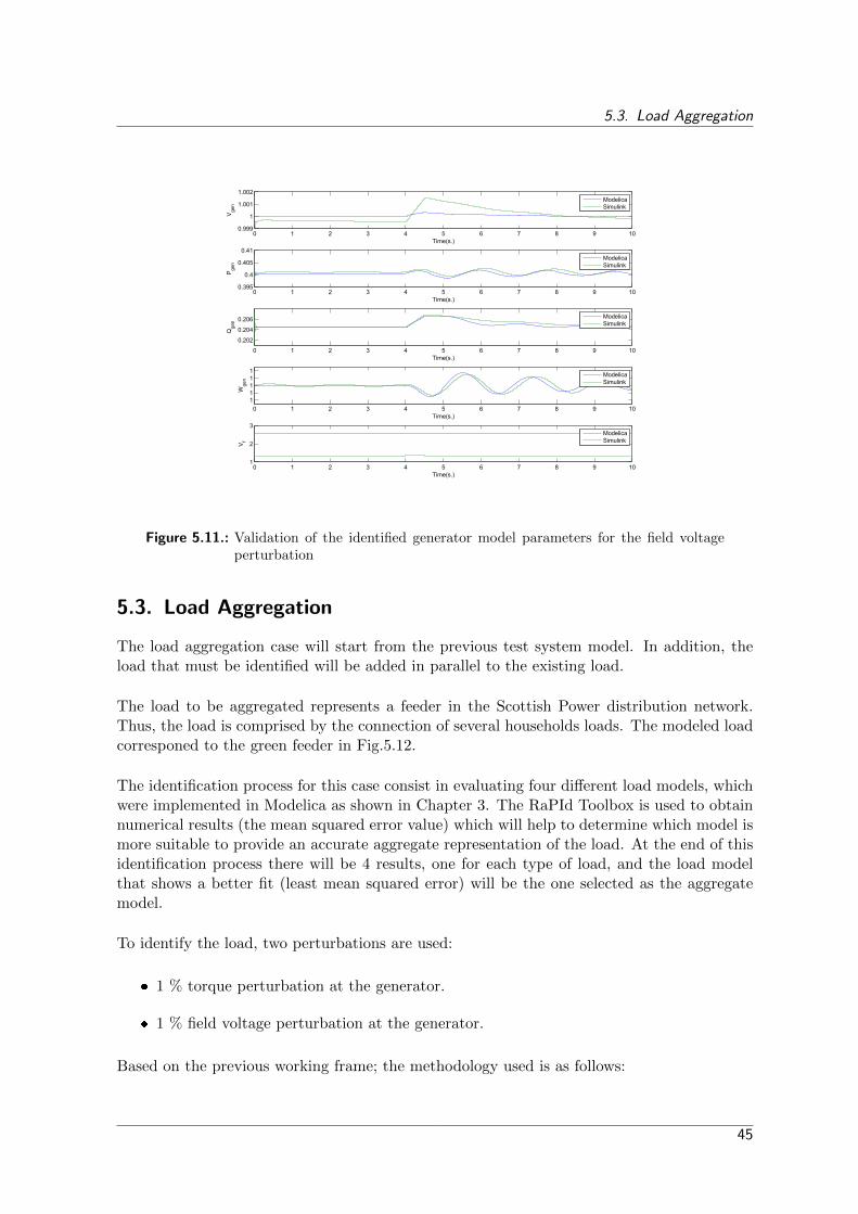
Figure 5.11.: Validation of the identified generator model parameters for the field voltageperturbation
5.3. Load Aggregation
The load aggregation case will start from the previous test system model. In addition, theload that must be identified will be added in parallel to the existing load.
The load to be aggregated represents a feeder in the Scottish Power distribution network.Thus, the load is comprised by the connection of several households loads. The modeled loadcorresponed to the green feeder in Fig.5.12.
The identification process for this case consist in evaluating four di↵erent load models, whichwere implemented in Modelica as shown in Chapter 3. The RaPId Toolbox is used to obtainnumerical results (the mean squared error value) which will help to determine which model ismore suitable to provide an accurate aggregate representation of the load. At the end of thisidentification process there will be 4 results, one for each type of load, and the load modelthat shows a better fit (least mean squared error) will be the one selected as the aggregatemodel.
To identify the load, two perturbations are used:
1 % torque perturbation at the generator.
1 % field voltage perturbation at the generator.
Based on the previous working frame; the methodology used is as follows:
45

5. Power System Model Identification
Figure 5.12.: Scottish Power distribution grid corresponding to the modeled load [3]
1. Collect measurement data: this is carried out with Simulink using the test system andadding the Scottish Power distribution network. The load to be identified representsthe green feeder in the Scottish Power distribution network [3].
2. Create the power system model in Modelica. The Modelica model created is shown inFig.5.13.
Load to be Identified
Figure 5.13.: Modelica model in the identification process
3. Compile an FMU from the Modelica model.
46

5.3. Load Aggregation
4. Create a Simulink model using the FMU block from the FMI Toolbox for Matlab.The one used is shown in Fig.5.14.
Figure 5.14.: RaPId Simulink model for the load aggregation case
5. Start the RaPId Toolbox.
6. Provide RaPId with settings (algorithm, parameters, variables, etc.): In these cases, toovercome the identification the same strategy described previously was used (PSO+Gradientdescent).
47

5. Power System Model Identification
5.3.1. Load Aggregate Model Identification Results
Exponential Recovery Load Model Results
The parameters resulting values and the corresponding error obtained from the identificationprocess can be found in Table 5.2:
Table 5.2.: Exponential recovery estimated aggregate load model parameters
Parameter Value
Active power time constant (Tp
) 1.3198Reactive power time constant (T
q
) 0.69108Static active power exponent (↵
s
) 9.5074Dynamic active power exponent (↵
t
) 2.3919Static reactive power exponent (�
s
) 8.5691Dynamic reactive power exponent (�
t
) 2.9145Mean squared error 1.8627e-007
The corresponding time domain simulation results comparing the reference data (generatedusing Simulink/SPS) and the Modelica simulation results are shown in Fig.5.15.
0 1 2 3 4 5 6 7 8 9 103.08
3.085
3.09
3.095
3.1x 10⁻³
Plo
ad
Time(s.)
ModelicaSimulink
0 1 2 3 4 5 6 7 8 9 101.5
1.502
1.504
1.506
1.508
1.51x 10⁻³
Qlo
ad
Time(s.)
ModelicaSimulink
(a) Torque perturbation
0 1 2 3 4 5 6 7 8 9 103.08
3.085
3.09
3.095
3.1x 10⁻³
Plo
ad
Time(s.)
ModelicaSimulink
0 1 2 3 4 5 6 7 8 9 101.5
1.502
1.504
1.506
1.508
1.51x 10⁻³
Qlo
ad
Time(s.)
ModelicaSimulink
(b) Field voltage perturbation
Figure 5.15.: Exponential recovery aggregate load model results
Discussion: All the parameters numerical values are positive and within an acceptable range.It can be observed that the static parameters are higher than the rest. The mean squarederror for this load is low, thus it means that the di↵erence between the reference data andthe Modelica aggregate load model is little. This is illustrated in Fig.5.15.
48

5.3. Load Aggregation
Voltage Dependent Aggregate Load Model Results
The parameters resulting values and the corresponding error obtained from the identificationprocess can be found in Table 5.3.
Table 5.3.: Voltage dependent estimated aggregate load model parameters
Parameter Value
Active power exponent (↵p
) 7.7454Reactive power exponent (↵
q
) 7.0214Mean squared error 2.8357e-007
The corresponding time domain simulation results comparing the reference data (generatedusing Simulink/SPS) and the Modelica simulation results are shown in Fig.5.16.
0 1 2 3 4 5 6 7 8 9 103.08
3.085
3.09
3.095
3.1x 10⁻³
Plo
ad
Time(s.)
ModelicaSimulink
0 1 2 3 4 5 6 7 8 9 101.5
1.502
1.504
1.506
1.508
1.51x 10⁻³
Qlo
ad
Time(s.)
ModelicaSimulink
(a) Torque perturbation
0 1 2 3 4 5 6 7 8 9 103.08
3.085
3.09
3.095
3.1x 10⁻³
Plo
ad
Time(s.)
ModelicaSimulink
0 1 2 3 4 5 6 7 8 9 101.5
1.502
1.504
1.506
1.508
1.51x 10⁻³
Qlo
ad
Time(s.)
ModelicaSimulink
(b) Field voltage perturbation
Figure 5.16.: Voltage dependent aggregate load model results
Discussion: All the parameters numerical values are positive and within an acceptable range.The active power exponent and the reactive power exponent are above 7, thus the variation ofthe active power and reactive power is very a↵ected by the voltage variation on the load. Themean squared error result for this load is low, thus it means that the di↵erence between thereference data and the Modelica aggregate load model is little. This is illustrated in Fig.5.16.
49

5. Power System Model Identification
Frequency Dependent Aggregate Load Model Results
The parameters resulting values and the corresponding error obtained from the identificationprocess can be found in Table 5.4.
Table 5.4.: Frequency dependent aggregate load model estimated parameters
Parameter Value
Active power voltage coe�cient (↵p
) 7.7576Active power frequency coe�cient (�
p
) -0.024682Reactive power voltage coe�cient (↵
q
) 7.0375Reactive power frequency coe�cient (�
q
) 0.02555Filter time constant (T
f
) 0.45296Mean squared error 3.3287e-007
The corresponding time domain simulation results comparing the reference data (generatedusing Simulink/SPS) and the Modelica simulation results are shown in Fig.5.17.
0 1 2 3 4 5 6 7 8 9 103.08
3.085
3.09
3.095
3.1x 10⁻³
Plo
ad
Time(s.)
ModelicaSimulink
0 1 2 3 4 5 6 7 8 9 101.5
1.502
1.504
1.506
1.508
1.51x 10⁻³
Qlo
ad
Time(s.)
ModelicaSimulink
(a) Torque perturbation
0 1 2 3 4 5 6 7 8 9 103.08
3.085
3.09
3.095
3.1x 10⁻³
Plo
ad
Time(s.)
ModelicaSimulink
0 1 2 3 4 5 6 7 8 9 101.5
1.502
1.504
1.506
1.508
1.51x 10⁻³
Qlo
ad
Time(s.)
ModelicaSimulink
(b) Field voltage perturbation
Figure 5.17.: Frequency dependent aggregate load model Results
Discussion: All the parameters numerical values are positive, except for (�p
), and withinan acceptable range. The negative value (�
p
) is correct, it means that the load active poweris inversely proportional to the frequency of the system. The active power voltage coe�cientand the reactive power voltage coe�cient are again above 7, thus the variation of the activepower and reactive power is very a↵ected by the voltage variation on the load. The meansquared error result for this load is medium, thus it means that the di↵erence between thereference data and the Modelica aggregate load model is higher than in the previous cases.This is illustrated in Fig.5.16.
50

5.3. Load Aggregation
ZIP aggregate load model Results
The parameters resulting values and the corresponding error obtained from the identificationprocess can be found in Table 5.5.
Table 5.5.: ZIP aggregate load model estimated parameters
Parameter Value
Constant Z coe�cient for active power (kpz
) 1Constant I coe�cient for active power (k
pi
) 0Constant P coe�cient for active power (k
pp
) 0Constant Z coe�cient for reactive power (k
qz
) 1Constant I coe�cient for reactive power (k
qi
) 0Constant P coe�cient for reactive power (k
qp
) 0Mean squared error 5.1415e-007
The ZIP load has one main characteristic:
kpz
+ kpi
+ kpp
= 1 (5.1)
RaPId allows to consider constraints in the form ( min < x < max ). To be able to take intoaccount the equality constraint in (5.1), a change of variables was used. Instead of working inthe Cartesian coordinate frame, the identification was held in the spherical coordinate frame,setting the constraints as shown in equations (5.2)-(5.4). (These constrains force the solutionspace to the first 1/8 of the sphere).
0 < r < 1 (5.2)
0 < ⇥ < ⇡/4 (5.3)
0 < � < ⇡/4 (5.4)
So the final expressions used to represent the constraints are:
kpz
= (rp
sin(⇥p
)cos(�p
))2 (5.5)
kpi
= (rp
sin(⇥p
)sin(�p
))2 (5.6)
kpi
= (rp
cos(⇥p
))2 (5.7)
This was performed similarly for the reactive power coe�cients equality constraints.
Discussion: The results show a completely constant impedance behavior of the aggregateload. The mean squared error result for this load are high, thus it means that di↵erencebetween the reference data and the Modelica aggregate load model is the highest. This isillustrated in Fig.5.16, where it can be observed that for the field voltage perturbation, theModelica system behaves completely di↵erent to the reference.
51

5. Power System Model Identification
0 1 2 3 4 5 6 7 8 9 103.08
3.085
3.09
3.095
3.1x 10⁻³
Plo
ad
Time(s.)
ModelicaSimulink
0 1 2 3 4 5 6 7 8 9 101.5
1.502
1.504
1.506
1.508
1.51x 10⁻³
Qlo
ad
Time(s.)
ModelicaSimulink
(a) Torque perturbation
0 1 2 3 4 5 6 7 8 9 103.08
3.085
3.09
3.095
3.1x 10⁻³
Plo
ad
Time(s.)
ModelicaSimulink
0 1 2 3 4 5 6 7 8 9 101.5
1.502
1.504
1.506
1.508
1.51x 10⁻³
Qlo
ad
Time(s.)
ModelicaSimulink
(b) Field voltage perturbation
Figure 5.18.: ZIP Results
Aggregate Load Model Identification Results Analysis
The results of the di↵erent loads are compared in Table 5.6:
Table 5.6.: Load Aggregation Error Comparison
Type of load Mean squared error
Exponential Recovery 1.8627e-007Voltage Dependent 2.8357e-007
Frequency Dependent 3.3287e-007ZIP 5.1415e-007
Based on the maximum fitness criteria (minimum mean squared error), the aggregate loadmodel that most matches the behavior of the data is the Exponential Recovery Load model.Further experiments can be performed in order to improve the aggregate load model responsecompared to the reference model. For example, instead of identifying load models indepen-dently, the identification could be done using a combination of load models in parallel andidentifying which percentage correspond to each type of load.
5.4. Photovoltaic Panel Parameter Estimation Case
The last parameter estimation case consist in estimating the parameters of a PV panel whenthere is an irradiation change and a temperature change. The results will be evaluated andstudied using statistical tools and concepts, such as the confidence interval.
To identify the PV, two perturbations will be performed:
Irradiation change from 1000 W/m2 to 500 W/m2 and back to 1000 W/m2 at t=[0.3-0.7].
52

5.4. Photovoltaic Panel Parameter Estimation Case
Temperature change from 25 �C to 40 �C and back to 25 �C at t=[0.3-0.7].
Based on the previous working frame; the methodology used is as follows:
1. Collect measurement data: this is carried out with Simulink using a reference modeldeveloped in Simulink.
2. Create the power system model in Modelica. The Modelica model created is shown inFig.5.19.
Figure 5.19.: Modelica model in the identification process.
3. Compile an FMU from the Modelica model.
4. Create a Simulink model using the FMU block from the FMI Toolbox for Matlab, seeFig.5.20. The only blocks required in order to simulate are: FMUme and Toworkspace.All data inputs and the scopes are included only to monitor the process interactively.
Figure 5.20.: RaPId Simulink model for the PV panel parameter identification
5. Start the RaPId Toolbox.
6. Provide RaPId with settings (algorithm, parameters, variables, etc.): In order to pro-ceed with the statistical analysis, the identification process has been performed 50 times
53

5. Power System Model Identification
using the genetic algorithm with di↵erent settings each time.
Note: the FMU memory issue still appeared, as a consequence, the settings were set toa number of approximately 130 iterations.
Photovoltaic Parameters Estimation Results
The parameters estimated were:
kv
: correction factor for the voltage.
ki
: correction factor for the current.
Fig.5.21 shows the results from 50 estimations and the statistical analysis for both variables.
It is important to notice that the amplitude of the confidence interval is inversely dependent onthe number of samples, that means, the bigger number of samples the narrower the interval is.
In this occasion, instead of performing the identification assessment based on the highest fit-ness criteria (minimum mean squared error), the assessment was performed through statisticalanalysis. The statistical analysis could be useful in order to evaluate the validity of the param-eter estimation results. For example, when the samples have a large variance, this indicatesthat a change in the parameter will have a negligible influence on the simulation output result.
Despite that repeating the estimation process several times o↵ers the opportunity to obtainmore information about the parameters estimated, it also requires more resources and time.It is important to take into account time consumption, a precise identification will requiretime because more iterations are required.
Finally, plotting the results using the mean value of the experiments, it is possible to observethis behaviour Fig.5.22.
54

5.4. Photovoltaic Panel Parameter Estimation Case
Figure 5.21.: Panel parameter identification statistical analysis
55

5. Power System Model Identification
0 0.1 0.2 0.3 0.4 0.5 0.6 0.7 0.8 0.9 134.99
34.995
35
35.005
VP
V
Time(s.)
ModelicaSimulink
0 0.1 0.2 0.3 0.4 0.5 0.6 0.7 0.8 0.9 12
2.5
3
3.5
4
4.5
5
VIV
Time(s.)
ModelicaSimulink
0 0.1 0.2 0.3 0.4 0.5 0.6 0.7 0.8 0.9 1500
600
700
800
900
1000
Irrad
iatio
n
Time(s.)
ModelicaSimulink
(a) Irradiation perturbation
0 0.1 0.2 0.3 0.4 0.5 0.6 0.7 0.8 0.9 134.99
34.995
35
35.005
VP
V
Time(s.)
ModelicaSimulink
0 0.1 0.2 0.3 0.4 0.5 0.6 0.7 0.8 0.9 14.57
4.575
4.58
4.585
VIV
Time(s.)
ModelicaSimulink
0 0.1 0.2 0.3 0.4 0.5 0.6 0.7 0.8 0.9 125
30
35
Tem
pera
ture
Time(s.)
ModelicaSimulink
(b) Temperature perturbation
Figure 5.22.: Panel parameter identification simulation results against reference data
56

6 Discussion
6.1. Modelica
Modelica potential relies in terms of a powerful mathematical language, the ability to unam-biguous model exchange and the numerical solvers which can solve very e�ciently complexsystems. Modelica is superior to other modeling tools because it allows, by using a simplemathematical language, the necessary tools to model high complexity models. In addition,the powerful mathematical solvers integrated in the Modelica simulation environments givesthe user the freedom to decide which methods to use in order to obtain the best results.Finally, Modelica has been proven to achieve the same results of other power system analysisspecific tools while providing new extra features.
6.1.1. Models
At the start of the thesis very few models were available and the existing library only hadsome very basic components, the first e↵ort was put to develop more models in order to beable to simulate more complex systems.
The models implemented in Modelica were based on previous existing models, either fromPSAT or Power Factory. These models were first designed for a software with di↵erent char-acteristics than Modelica and they have been adapted. Despite the results of adapting themodels are very positive, Modelica brings us the opportunity to create new models using allthe Modelica tools. What this implies is that developing completely new models in Modelicaspecially designed according the Modelica language and the functionalities it provides canlead to more flexibility and better simulation performance.
Actually, some software companies are developing libraries which use the whole Modelicafunctionalities. The problem is that these libraries are protected and proprietary. It wouldbe very interesting to dispose of an Open Source library for power systems that uses all thepotential o↵ered by Modelica.
6.1.2. Model Exchange
Modelica does not just provide tools to create models, the magic of Modelica comes in termsof reutilization and sharing. The fact that any Modelica model can be converted to an FMU
57

6. Discussion
and then be able to run in di↵erent softwares is a revolution. The use of Modelica for powersystems modeling will help to stop the infinite conversions of model from software-to-software.These software-to-software conversions are not only time consuming, but they might also leadto possible simulation problems (including possible lost of information due to simplifications).
Nowadays, there are dozens of power systems simulation and analysis tools, but the problemis that they are incompatible. For example, a model that runs in Power Factory cannot runin Simulink. This fact generates tensions when organizations which use di↵erent tools mustcollaborate and this can be translated into actual economic losses. Modelica could bring thesolution to this problem, but it would require time, pro activity and international acceptance.
One of the problems in the power system community is the reticence to change. Every orga-nization uses their own tools and may not trust the other tools. With Modelica this problemcould be avoided. Fortunately, everyday Modelica is getting more popular and seen morereliable since it is used in many industrial applications including complex dynamic systemmodeling (which is of relevance for power system modeling).
The e↵orts made in this thesis to perform software-to-software validation serve as evidence togive the power systems community that Modelica tools are capable of producing the same sim-ulation results than domain specific tools while at the same time providing additional benefits.
6.2. System Identification
6.2.1. RaPId Toolbox
The thesis was the first practical use of the RaPId toolbox, so its main features and its char-acteristics were tested. The usage of the RaPId toolbox lead to interesting results.
Evaluation of the RaPId toolbox: RaPId did an excellent job and made available manyoptimization tools related to the identification problem solved in this thesis. The toolboxis also easy to use. In addition, the iTesla RaPId Toobox is free for modification which isbeneficial in comparison to Matlab optimization Toolbox.
Possible Improvements: One major improvement which could be attempted is to allowthe user to submit more elaborate parameter constraints, instead of only the min and maxconstrains available.
6.2.2. Thesis Results
The system identification and the parameter estimation cases could not be performed as itwas intended due to the memory handing bug found in the FMUs generated by Dymola.
Due to this di�culty the process became more time consuming, so a strategy had to bedeveloped to perform parameter estimation and model aggregation. The estimation process
58

6.2. System Identification
should always be evaluated according to a performance indicator, i.e. an assessment criteria.During the thesis two assessment criteria were utilized:
Best fitness (least mean squared error).
Statistical analysis.
Despite that the best fitness strategy is faster and easier, the statistical analysis of the ex-periment can provide more useful information. Even if the statistical method is not used theestimation should always be performed several times with di↵erent settings in order to havea better confidence in the estimates.
The parameter estimation carried out in the thesis o↵ers good results. The most challengingcase was to estimate the parameters of the generator.
Estimation of the generator parameters: This was the most interesting estimation caseof the thesis, due to the need for of a physical understanding of the variation of the pa-rameters, as well as, the complexity it presents (7 parameters). In this estimation case theinfluence of the FMU bug was notorious and it could a↵ect the results. The methodology usedto cope with the bug o↵ers good results. It would be desirable to run the standard estimationprocedure and compare results. A full standard estimation procedure for this model couldrequire intensive calculations, and thus, could lead to more accurate results.
Aggregate load model identification: The results shown the type of load that mostresembles the reference data was the exponential recovery load. It would be interesting toattempt another approach such as a combination of load models in parallel and identifyingwhich percentage correspond to each type of load. It was also pointed out when experiment-ing with the ZIP load model, that by using a change of variables, the constrains could beadded into the model without the need of implementing them in the software.
Solar photovoltaic parameter estimation: The statistical analysis of the data showed acontrast in the previous methodology. In practice it is di�cult to ensure that a parameterhas a value constant in time, so the fact of providing a confidence interval is very relevant.It is important to provide a confidence interval because there is always measurement noisein the reference signal, as well due to the fact the optimization algorithm will always stop atsome error. In addition, a 95 % confidence interval is good enough to provide the precision,accuracy and security necessary for phasor time domain simulations.
59


7 Conclusion and Future Work
7.1. Conclusions
The thesis o↵ers a proof of the suitability of Modelica for power systems modeling and thepotential of the FMI standard. The modeling of power systems and the identification casesusing the FMUs were very successful. This success is a foundation for future work allowingthe start of a new power systems modeling trend.
During the thesis the Modelica language was learned and by using this knowledge complex,models could be implemented. That by developing models in Modelica, the author learnedhow the models work in detail, not just how to use them, as it could happen when using aninbuilt library typical of most power system simulation tools.
Best practices in power systems modeling using Modelica and system identification usingRaPId were identified, these practices are the product of the author’s own experience. Futuremodel developers are encouraged to update them and to increae their complexity.
The parameter estimation procedure o↵ers not only the value of estimating the parameters, itis also a success in terms of model exchange and the usage of the FMI standard. This featurethat is provided in Modelica tools has a lot of potential and further applications should beinvestigated.
7.2. Future Work
Future work on the Modelica aspects of this thesis would be the conception of a power systemsopen source library specially designed and adapted to the Modelica language and a powerflow solver tool. New models should be especially formulated for Modelica. This would allowfor example, 3-phase modeling together with positive sequence modeling using the facilitiesprovided by MetaModelica.
61


Bibliography
[1] A. S. Chieh, P. Panciatici, and J. Picard, “Power system modeling in modelica for time-domain simulation,” in 2011 IEEE Trondheim, PowerTech, pp. 1–8, IEEE, 2011.
[2] F. Milano, Power System Analysis Toolbox Documentation for PSAT. version 2.1.8, 2013.
[3] A. Collison, “High penetration of PV systems at Hoel Glyndwr.” SP Energy Networks,2012.
[4] L. Vanfretti, W. Li, T. Bogodorova, and P. Panciatici, “Unambiguous power systemdynamic modeling and simulation,” PESGM2013.
[5] R. G. Sargent, “Verification and validation of simulation models,” in Proceedings of the37th conference on Winter simulation, pp. 130–143, Winter Simulation Conference, 2005.
[6] H. Elmqvist, S. E. Mattsson, and M. Otter, “Modelica: The new object-oriented model-ing language,” in 12th European Simulation Multiconference, Manchester, UK, 1998.
[7] T. Bogodorova, M. Sabate, G. Leon, L. Vanfretti, M. Halat, J. Heyberger, and P. Panci-atici, “A modelica power system library for phasor time-domain simulation,” ISGT2013.
[8] A. S. Chieh, P. Panciatici, and J. Picard, “Power system modeling in modelica for time-domain simulation,” in 2011 IEEE Trondheim, PowerTech, pp. 1–8, IEEE, 2011.
[9] P. A. Fritzson, Principles of object-oriented modeling and simulation with Modelica 2.1.IEEE press, 2004.
[10] I. R. Navarro, M. Larsson, and G. Olsson, “Object-oriented modeling and simulationof power systems using modelica,” in Power Engineering Society Winter Meeting, 2000.IEEE, vol. 1, pp. 790–795, IEEE, 2000.
[11] J. Machowski, J. W. Bialek, and J. R. Bumby, Power System Dynamics. Jhone Wileyand Sons, 1997.
[12] S. He, Modeling power system load using intelligent methods. PhD thesis, Kansas StateUniversity, 2011.
[13] F. Mahmood, “Improving the photovoltaic model in powerfactory,” Master’s thesis,KTH, 2012.
[14] L. Ljung, System identification. Wiley Online Library, 1999.
[15] W. Forst and D. Ho↵mann, Optimization: theory and practice. Springer, 2010.
63

Bibliography
[16] D. Pierre, Optimization theory with applications. DoverPublications. com, 1969.
[17] J. Kennedy, “Particle swarm optimization,” in Encyclopedia of Machine Learning,pp. 760–766, Springer, 2010.
[18] C. R. Houck, J. A. Joines, and M. G. Kay, “A genetic algorithm for function optimization:a matlab implementation,” NCSU-IE TR, vol. 95, no. 09, 1995.
[19] X. Deng, “System identification based on particle swarm optimization algorithm,” inComputational Intelligence and Security. International Conference on, vol. 1, pp. 259–263, IEEE, 2009.
[20] Modelon AB, FMI Toolbox User’s Guide 1.5. Self publishing, 2013.
[21] T. Blochwitz, M. Otter, M. Arnold, C. Bausch, C. Clauß, H. Elmqvist, A. Junghanns,J. Mauss, M. Monteiro, T. Neidhold, et al., “The functional mockup interface for tool in-dependent exchange of simulation models,” in Modelica’2011 Conference, March, pp. 20–22, 2011.
[22] C. Schubert, T. Neidhold, and G. Kunze, “Experiences with the new FMI standardselected applications at Dresden university,” in Modelica Conference, p. 94, 2011.
[23] The Modelica Association, “Functional mock-up interface.” https://www.fmi-standard.org, August 2013.
[24] S. Singer and J. Nelder, “Nelder-mead algorithm,” Scholarpedia, vol. 4, no. 7, p. 2928,2009.
64

AAppendix
A.1. Software-to-Software Model Validation Results
0 5 10 150.2
0.22
0.24
0.26
0.28
0.3
0.32
G Gen
erat
or-T
3
Time(s.)
PSATModelica
0 5 10 150.01
0.011
0.012
0.013
0.014
0.015
0.016
T 1-3
Time(s.)
PSATModelica
0 5 10 150.997
0.998
0.999
1
1.001
Z
Time(s.)
PSATModelica
0 5 10 150.96
0.97
0.98
0.99
1
1.01
1.02
V1
Time(s.)
PSATModelica
0 5 10 151.203
1.2035
1.204
1.2045
1.205
1.2055
v f
Time(s.)
PSATModelica
0 5 10 150.1595
0.16
0.1605
0.161
0.1615
0.162
0.1625
Pm
Time(s.)
PSATModelica
0 5 10 150.16
0.17
0.18
0.19
0.2
0.21
0.22
P1
Time(s.)
PSATModelica
0 5 10 150.118
0.12
0.122
0.124
0.126
Q1
Time(s.)
PSATModelica
Figure A.1.: Second order synchronous machine software-to-software validation
65

A. Appendix
0 5 10 15
0.65
0.7
0.75
0.8
G Gen
erat
or-T
3
Time(s.)
PSATModelica
0 5 10 150.01
0.011
0.012
0.013
0.014
0.015
0.016
T 1-3
Time(s.)
PSATModelica
0 5 10 151.1
1.105
1.11
1.115
E´ q
Time(s.)
PSATModelica
0 5 10 150.997
0.998
0.999
1
1.001
Z
Time(s.)
PSATModelica
0 5 10 150.98
0.99
1
1.01
1.02
1.03
V1
Time(s.)
PSATModelica
0 5 10 152.614
2.615
2.616
2.617
2.618
Vf
Time(s.)
PSATModelica
0 5 10 150.1595
0.16
0.1605
0.161
0.1615
0.162
0.1625
Pm
Time(s.)
PSATModelica
0 5 10 150.16
0.17
0.18
0.19
0.2
0.21
0.22
P1
Time(s.)
PSATModelica
0 5 10 150.118
0.119
0.12
0.121
0.122
0.123
0.124
Q1
Time(s.)
PSATModelica
Figure A.2.: Third order synchronous machine software-to-software validation
0 1 2 3 4 5 6 7 8 9 101.104
1.106
1.108
1.11
1.112
1.114
1.116
e´q
Time(s.)
PSATModelica
0 1 2 3 4 5 6 7 8 9 100.985
0.99
0.995
1
1.005
1.01
1.015
V1
Time(s.)
PSATModelica
0 1 2 3 4 5 6 7 8 9 102
2.2
2.4
2.6
2.8
3
v f
Time(s.)
PSATModelica
Figure A.3.: Automatic voltage regulator software-to-software validation
66

A.1. Software-to-Software Model Validation Results
0 2 4 6 8 101.095
1.1
1.105
1.11
1.115
1.12e´
q
Time(s.)
PSATModelica
0 2 4 6 8 100.997
0.998
0.999
1
1.001
Z
Time(s.)
PSATModelica
0 2 4 6 8 100.97
0.98
0.99
1
1.01
1.02
1.03
V1
Time(s.)
PSATModelica
0 2 4 6 8 102.61
2.612
2.614
2.616
2.618
v f
Time(s.)
PSATModelica
0 2 4 6 8 100.15
0.155
0.16
0.165
0.17
Pm
Time(s.)
PSATModelica
Figure A.4.: Turbine governor software-to-software validation
0 5 100.437
0.4371
0.4371
0.4372
G Gen
erat
or-T
3
Time(s.)
PSATModelica
0 5 101
1.0002
1.0004
1.0006
1.0008
1.001
Z
Time(s.)
PSATModelica
0 5 100.9933
0.9933
0.9934
0.9934
0.9935
0.9935
0.9936
V3
Time(s.)
PSATModelica
0 5 101.7175
1.718
1.7185
1.719
1.7195
1.72
v f
Time(s.)
PSATModelica
0 5 100.079
0.0795
0.08
0.0805
0.081
0.0815
0.082
Pm
Time(s.)
PSATModelica
0 5 100.06
0.065
0.07
0.075
0.08
0.085
0.09
P3
Time(s.)
PSATModelica
0 5 100.04
0.05
0.06
0.07
0.08
0.09
Q3
Time(s.)
PSATModelica
Figure A.5.: Constant P,Q load software-to-software validation
67
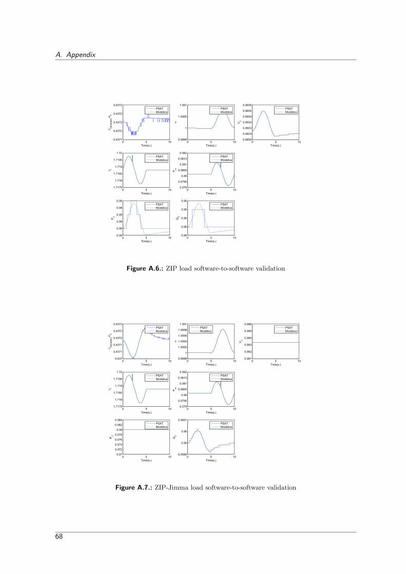
A. Appendix
0 5 100.4371
0.4372
0.4372
0.4372
0.4372G G
ener
ator
-T3
Time(s.)
PSATModelica
0 5 100.9995
1
1.0005
1.001
Z
Time(s.)
PSATModelica
0 5 100.9932
0.9933
0.9933
0.9934
0.9934
0.9935
0.9935
V3
Time(s.)
PSATModelica
0 5 101.7175
1.718
1.7185
1.719
1.7195
1.72
v f
Time(s.)
PSATModelica
0 5 100.079
0.0795
0.08
0.0805
0.081
0.0815
0.082
Pm
Time(s.)
PSATModelica
0 5 100.08
0.08
0.08
0.08
0.08
0.08
P3
Time(s.)
PSATModelica
0 5 100.06
0.06
0.06
0.06
0.06
Q3
Time(s.)
PSATModelica
Figure A.6.: ZIP load software-to-software validation
0 5 100.437
0.4371
0.4371
0.4372
0.4372
0.4373
G Gen
erat
or-T
3
Time(s.)
PSATModelica
0 5 100.9998
1
1.0002
1.0004
1.0006
1.0008
1.001
Z
Time(s.)
PSATModelica
0 5 100.991
0.992
0.993
0.994
0.995
0.996
V3
Time(s.)
PSATModelica
0 5 101.7175
1.718
1.7185
1.719
1.7195
1.72
v f
Time(s.)
PSATModelica
0 5 100.079
0.0795
0.08
0.0805
0.081
0.0815
0.082
Pm
Time(s.)
PSATModelica
0 5 100.07
0.072
0.074
0.076
0.078
0.08
0.082
0.084
P3
Time(s.)
PSATModelica
0 5 100.0599
0.06
0.06
0.0601
Q3
Time(s.)
PSATModelica
Figure A.7.: ZIP-Jimma load software-to-software validation
68

A.1. Software-to-Software Model Validation Results
0 5 100.4372
0.4372
0.4372
0.4372
0.4372
0.4372G G
ener
ator
-T3
Time(s.)
PSATModelica
0 5 100.9995
1
1.0005
1.001
Z
Time(s.)
PSATModelica
0 5 100.9932
0.9933
0.9933
0.9934
0.9934
0.9935
V3
Time(s.)
PSATModelica
0 5 101.7175
1.718
1.7185
1.719
1.7195
1.72
v f
Time(s.)
PSATModelica
0 5 100.079
0.0795
0.08
0.0805
0.081
0.0815
0.082
Pm
Time(s.)
PSATModelica
0 5 100.08
0.08
0.08
0.08
0.08
0.08
P3
Time(s.)
PSATModelica
0 5 100.06
0.06
0.06
0.06
0.06
Q3
Time(s.)
PSATModelica
Figure A.8.: Voltage dependent load software-to-software validation
0 5 100.4372
0.4372
0.4372
0.4372
0.4372
G Gen
erat
or-T
3
Time(s.)
PSATModelica
0 5 100.9995
1
1.0005
1.001
Z
Time(s.)
PSATModelica
0 5 100.9932
0.9933
0.9933
0.9934
0.9934
0.9935
V3
Time(s.)
PSATModelica
0 5 101.7175
1.718
1.7185
1.719
1.7195
1.72
v f
Time(s.)
PSATModelica
0 5 100.079
0.0795
0.08
0.0805
0.081
0.0815
0.082
Pm
Time(s.)
PSATModelica
0 5 100.0801
0.0801
0.0801
0.0801
0.0801
P3
Time(s.)
PSATModelica
0 5 100.057
0.057
0.057
0.057
0.057
0.057
Q3
Time(s.)
PSATModelica
Figure A.9.: Exponential recovery load software-to-software validation
69

A. Appendix
0 5 100.437
0.4371
0.4372
0.4373
0.4374
0.4375
0.4376G G
ener
ator
-T3
Time(s.)
PSATModelica
0 5 100.9998
1
1.0002
1.0004
1.0006
1.0008
Z
Time(s.)
PSATModelica
0 5 100.993
0.9932
0.9934
0.9936
0.9938
V3
Time(s.)
PSATModelica
0 5 101.7175
1.718
1.7185
1.719
1.7195
1.72
v f
Time(s.)
PSATModelica
0 5 100.079
0.0795
0.08
0.0805
0.081
0.0815
0.082
Pm
Time(s.)
PSATModelica
0 5 100.08
0.08
0.08
0.08
0.0801
0.0801
0.0801
P3
Time(s.)
PSATModelica
0 5 100.06
0.06
0.06
0.06
0.0601
Q3
Time(s.)
PSATModelica
Figure A.10.: Frequency dependent load software-to-software validation
0 5 100.4365
0.437
0.4375
0.438
0.4385
0.439
0.4395
G Gen
erat
or-T
3
Time(s.)
PSATModelica
0 5 100.9996
0.9998
1
1.0002
1.0004
1.0006
Z
Time(s.)
PSATModelica
0 5 100.9915
0.992
0.9925
0.993
0.9935
0.994
V3
Time(s.)
PSATModelica
0 5 101.7175
1.718
1.7185
1.719
1.7195
1.72
v f
Time(s.)
PSATModelica
0 5 100.079
0.0795
0.08
0.0805
0.081
0.0815
0.082
Pm
Time(s.)
PSATModelica
0 5 100.0796
0.0798
0.08
0.0802
0.0804
0.0806
0.0808
P3
Time(s.)
PSATModelica
0 5 100.0596
0.0598
0.06
0.0602
0.0604
0.0606
0.0608
Q3
Time(s.)
PSATModelica
Figure A.11.: Mixed load software-to-software validation
70

A.1. Software-to-Software Model Validation Results
0 2 4 6 8 100.058
0.06
0.062
0.064
0.066
Slip
Time(s.)
PSATModelica
0 2 4 6 8 10
0.65
0.7
0.75
0.8
G Gen
erat
or-T
3
Time(s.)
PSATModelica
0 2 4 6 8 100.012
0.014
0.016
0.018
0.02
T 1-T3
Time(s.)
PSATModelica
0 2 4 6 8 100.95
0.96
0.97
0.98
0.99
1
1.01
V1
Time(s.)
PSATModelica
0 2 4 6 8 100.94
0.95
0.96
0.97
0.98
0.99
1
V3
Time(s.)
PSATModelica
0 2 4 6 8 10-0.102
-0.101
-0.1
-0.099
-0.098
-0.097
-0.096
P3
Time(s.)
PSATModelica
0 2 4 6 8 10-0.057
-0.056
-0.055
-0.054
-0.053
Q3
Time(s.)
PSATModelica
Figure A.12.: Induction machine software-to-software validation
0 5 100.2
0.25
0.3
0.35
0.4
0.45
0.5
G Gen
erat
or-T
3
Time(s.)
PSATModelica
0 5 100.9975
0.998
0.9985
0.999
0.9995
1
1.0005
1.001
1.0015
1.002
Z
Time(s.)
PSATModelica
0 5 100.0295
0.03
0.0305
0.031
0.0315
0.032
0.0325
I d
Time(s.)
PSATModelica
0 5 100.038
0.0385
0.039
0.0395
0.04
I q
Time(s.)
PSATModelica
0 5 100.92
0.94
0.96
0.98
1
1.02
1.04
V1
Time(s.)
PSATModelica
0 5 100.92
0.94
0.96
0.98
1
1.02
1.04
V3
Time(s.)
PSATModelica
Figure A.13.: Constant P Q generator software-to-software validation
71

A. Appendix
0 2 4 6 8 10-0.04
-0.02
0
0.02
0.04
0.06
0.08
0.1
x
Time(s.)
PSATModelica
0 2 4 6 8 100.01
0.015
0.02
0.025
0.03
0.035
0.04
0.045
0.05
I d
Time(s.)
PSATModelica
0 2 4 6 8 10-0.01
0
0.01
0.02
0.03
0.04
0.05
I q
Time(s.)
PSATModelica
0 2 4 6 8 100.96
0.97
0.98
0.99
1
1.01
1.02
1.03
1.04
V3
Time(s.)
PSATModelica
0 2 4 6 8 100.039
0.04
0.041
0.042
0.043
0.044
0.045
0.046
0.047
P3
Time(s.)
PSATModelica
0 2 4 6 8 100
0.005
0.01
0.015
0.02
0.025
0.03
0.035
0.04
0.045
Q3
Time(s.)
PSATModelica
Figure A.14.: Constant P V generator software-to-software validation
0 0.1 0.2 0.3 0.4 0.5 0.6 0.7 0.8 0.9 1
0.99951
1.00051.001
V (p
.u.)
Time(s.)
PowerFactoryModelica
0 0.1 0.2 0.3 0.4 0.5 0.6 0.7 0.8 0.9 10
1
2
Ang
le (d
eg.)
Time(s.)
PowerFactoryModelica
0 0.1 0.2 0.3 0.4 0.5 0.6 0.7 0.8 0.9 10
0.5
P (M
W)
Time(s.)
PowerFactoryModelica
0 0.1 0.2 0.3 0.4 0.5 0.6 0.7 0.8 0.9 1-0.01
0
0.01
Q (M
Var
)
Time(s.)
PowerFactoryModelica
0 0.1 0.2 0.3 0.4 0.5 0.6 0.7 0.8 0.9 10
0.5
1
Id (p
.u.)
Time(s.)
PowerFactoryModelica
0 0.1 0.2 0.3 0.4 0.5 0.6 0.7 0.8 0.9 1-0.02
0
0.02
Iq (p
.u.)
Time(s.)
PowerFactoryModelica
Figure A.15.: KTH PV model software-to-software validation (Irradiation change)
72

A.1. Software-to-Software Model Validation Results
0 0.1 0.2 0.3 0.4 0.5 0.6 0.7 0.8 0.9 11.0003
1.0003
1.0003
V (p
.u.)
Time(s.)
PowerFactoryModelica
0 0.1 0.2 0.3 0.4 0.5 0.6 0.7 0.8 0.9 11.73
1.74
1.75
Ang
le (d
eg.)
Time(s.)
PowerFactoryModelica
0 0.1 0.2 0.3 0.4 0.5 0.6 0.7 0.8 0.9 10.445
0.45
P (M
W)
Time(s.)
PowerFactoryModelica
0 0.1 0.2 0.3 0.4 0.5 0.6 0.7 0.8 0.9 10
0.5
1x 10⁻⁴
Q (M
Var
)
Time(s.)
PowerFactoryModelica
0 0.1 0.2 0.3 0.4 0.5 0.6 0.7 0.8 0.9 10.895
0.9
0.905
Id (p
.u.)
Time(s.)
PowerFactoryModelica
0 0.1 0.2 0.3 0.4 0.5 0.6 0.7 0.8 0.9 1-2
-1
0x 10-4
Iq (p
.u.)
Time(s.)
PowerFactoryModelica
Figure A.16.: KTH PV model software-to-software validation (Temperature change)
73