From Proc. AIAA Comp. in Aerospace 10 Conf. , March 28-30, 1995, San Antonio, TX.

UltraSAN VERSION 3: ARCHITECTURE, FEATURES, AND

IMPLEMENTATION �

W. H. Sandersy, W. D. Obal IIz, M. A. Qureshiy, and F. K. Widjanarkoz

y Center for Reliable and High-Performance Computing

Coordinated Science Laboratory

University of Illinois at Urbana-Champaign

Urbana, IL 61801

fwhs, qureshig@crhc.uiuc.edu

z Dept. of Electrical and Computer Engineering

University of Arizona

Tucson, AZ 85721

fobal, krisnadig@ece.arizona.edu

Abstract

This paper describes version three of UltraSAN, asoftware environment for the performance, depend-ability, and performability evaluation of computer net-works and systems. The package makes use of bothanalytic- and simulation-based solution methods usinga single, high-level, representation known as stochas-tic activity networks. Version three, just completed,contains signi�cant enhancements, relative to the ear-lier versions, in model speci�cation, construction, andsolution.

Keywords: Stochastic Petri Nets, Stochastic Ac-tivity Networks, Model-Based Evaluation, Perfor-mance, Dependability, Performability.

1 IntroductionDevelopment of tool-based techniques for perfor-

mance/dependability evaluation, and in turn, thetools themselves, is an active research area. This pa-per describes version three of UltraSAN, one such toolwith this aim. In UltraSAN, models are speci�ed us-ing a variant of stochastic Petri nets (SPNs) knownas stochastic activity networks (SANs), and solutiontechniques include many analytic- and simulation-based approaches. Other SPN-based tools with thisaim include, among many, DSPNexpress [1], FI-GARO [2], GreatSPN [3], METASAN [4], RDPS [5],

�This work was supported in part by IBM, Motorola SatelliteCommunications, and US West Advanced Technologies.

SPNP [6], SURF-2 [7], TimeNET [8], and Ultra-

SAN [9].

Version three of UltraSAN has many enhancementsrelative to the initial version, which is described in[9]. In particular, with respect to the user interface,a parameterized model speci�cation method that fa-cilitates solution of models with multiple sets of inputparameter values has been developed. Furthermore,three new analytical solvers, as well as a terminatingsimulation solver based on importance sampling, havebeen added to the package.

The �rst new analytic solver solves models thathave deterministic as well as exponential activities.The two remaining new analytic solvers compute theprobability distribution function, and mean, respec-tively, of reward accumulated over a �nite interval.The importance sampling simulator provides, in manycases, an e�cient solution for models that containrare events which are signi�cant relative to a measurein question. These enhancements have signi�cantlyimproved UltraSAN's usefulness to others, and illus-trated its e�ectiveness as a test-bed for new modelingtechniques. The package has now been at academicand industrial sites for about four years, and muchhas been learned from its use.

The remainder of the paper is organized as follows.Section II of this paper gives an overview of the mod-eling process, as embodied in UltraSAN, including abrief review of SANs and an example to illustrate theuse of SANs in modeling a simple multiprocessor. The

intent here is to provide a high-level overview of the ca-pabilities and features of the package, without clutter-ing the discussion with too many details of any singleaspect. In Sections III{V, each step of the modelingprocess is described in detail. These sections providemore insight regarding the design choices that weremade in each step of the process. Finally, Section VIsummarizes the contributions and features of the tool,and suggests areas of future research and development.

2 Organization

The organization of UltraSAN follows directly fromthe goals of the package: the desire to create an envi-ronment (test-bed) for experimenting with new modelconstruction and solution techniques, and the goal offacilitating large-scale evaluations of realistic systemsusing both analytic- and simulation-based techniques.The �rst goal dictates that the software be constructedin a modular fashion, so new construction and solutiontechniques can be easily added. The second goal dic-tates that many di�erent solution techniques be avail-able, since no single technique is ideal in all circum-stances.

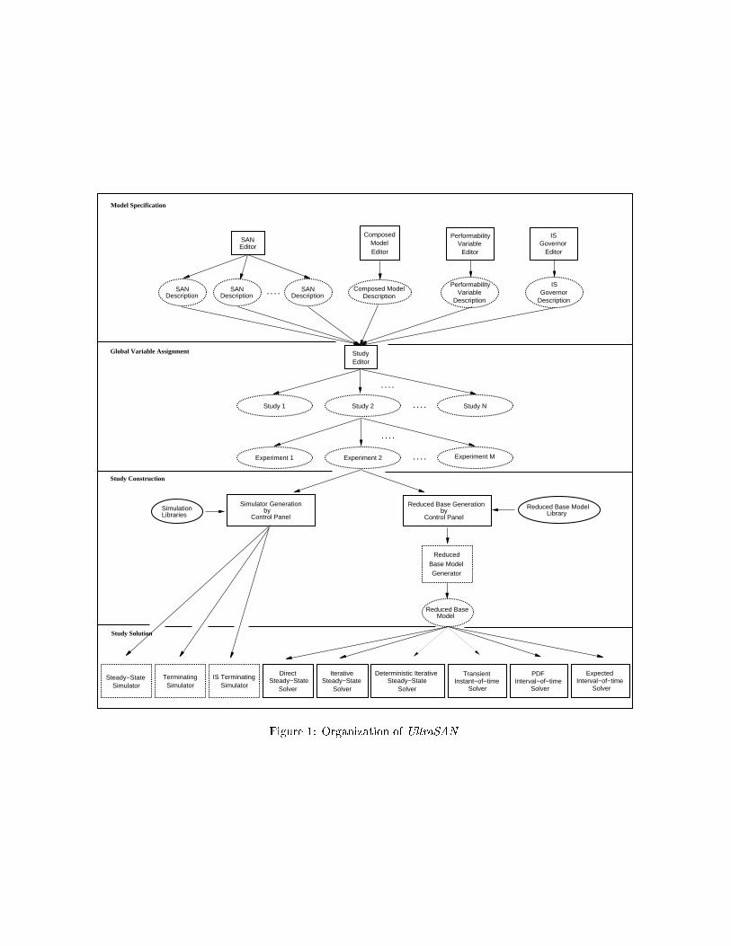
As shown in Figure 1, the package is constructed ina modular manner. All of the modules shown are coor-dinated by a central program called the control panel,that manages the interface between the user and thevarious modules, and provides basic consistency check-ing. In addition, the control panel o�ers several usefulutilities, such as automatic documentation and conve-nient viewing of output data. The modules commu-nicate via �les which have well-de�ned formats. Thiscon�guration makes it easy to add new functionality,thus contributing to the goal of being a test-bed fordeveloping new modeling techniques.

Figure 1 is divided into four sections, represent-ing the four phases of the modeling process used inUltraSAN : model speci�cation, global variable assign-

ment, study construction, and study solution. Thesephases are brie y described here as an introductionto the package, with more elaborate descriptions oftheir functioning and underlying theory given in thefollowing sections.

Model speci�cation The �rst phase of the model-ing process is model speci�cation. In this phase, SANsare de�ned graphically using the SAN editor and thencomposed into a hierarchical model using the com-posed model editor. The performance variable editoris then used to de�ne the performance measures ofinterest in terms of a reward structure at the SANlevel. Once a model is speci�ed, it is typically solvedmany times for di�ering values of the input parame-

ters. To accommodate this activity, UltraSAN allowsmodel speci�cations to be parameterized through theuse of global variables in de�nitions of model compo-nents in the SAN editor.

Global variable assignment Global variable as-signment, the second phase of the modeling process,is carried out by the study editor. In this phase, valuesare assigned to global variables. A model speci�cation,together with the assignment of a single value to eachglobal variable, is called an experiment. A group ofrelated experiments is called a study. UltraSAN pro-vides the study editor to make it easy to specify groupsof related experiments.

Study construction The third phase of the model-ing process, study construction, is the process of con-verting a speci�ed model and a global variable assign-ment into a format amenable to computer solution viaanalytic or simulation-based techniques.

Analytical models are constructed by automaticallygenerating a Markov process representation of themodel. The size of the generated Markov process isdetermined in part by the de�nition of state. In stan-dard stochastic Petri net models, the typical de�ni-tion of the state space is the set of tangible reachablemarkings. Realistic models of modern systems usu-ally have very large state spaces. This problem hasbeen widely recognized, and various approaches havebeen devised to handle the explosive growth [10, 11].UltraSAN uses an innovative largeness-avoidance ap-proach called reduced base model construction [12].This technique uses information about the perfor-mance measures and symmetries in the model to di-rectly generate a stochastic process that is often muchsmaller than the set of reachable markings, and yet issu�cient to support the speci�ed performance mea-sures. Experience has shown that reduced base modelconstruction is e�ective for medium to large systemsthat have replicated subsystems [13].

When the developed model is intended to be solvedusing simulation, UltraSAN does not generate a state-level representation. For this solution method, studyconstruction is accomplished by linking the model de-scription �les generated in model speci�cation andglobal variable assignment to the simulation library.The result is an executable simulation of the model.Essentially, simulation is accomplished by assigningevents to activity completions and using the rules ofSAN execution to determine the next state. The sim-ulation is made more e�cient through the use of datastructures designed for reduced base model construc-tion [14]. Symmetries in the model that allow lumping

SANEditor

ComposedModelEditor

ISGovernor

Editor

Composed ModelDescription Variable

Description

PerformabilitySAN

DescriptionSAN

Description. . . .SANDescription

ReducedBase ModelGenerator

Reduced Base Model

StudyEditor

. . . .

. . . .

. . . .

. . . .

Reduced Base Generation by Control Panel

Model Specification

Global Variable Assignment

Study Construction

Study Solution

TerminatingSimulator

Reduced Base Model Library

Simulator Generation by Control Panel

Study 1 Study 2 Study N

Experiment 1 Experiment 2

SimulatorSteady−State

Direct

SolverSteady−State

Iterative

SolverSteady−State

Deterministic Iterative

SolverSteady−State

Solver

TransientInstant−of−time Interval−of−time

Solver

SimulationLibraries

IS TerminatingSimulator

PerformabilityVariable

Editor

GovernorDescription

IS

Experiment M

Interval−of−timeSolver

ExpectedPDF

Figure 1: Organization of UltraSAN.

in state space construction are also useful for reduc-ing the amount of future events list management thatmust be done for each state change.

Study construction is carried out using the controlpanel. After verifying that the model description iscomplete, the control panel builds the reduced basemodel generator for each experiment to be solved an-alytically, and builds executable simulators for experi-ments where simulation-based solution is desired. Thecontrol panel can then be used to run the reducedbase model generator for all experiments that are tobe solved analytically. In this case, the control panelcan distribute the jobs to run on a user-speci�ed list ofother available machines. This \multiple runs" featuremakes it easy to construct a study with little e�ort onthe part of the user.

Study solution The last phase of the modeling pro-cess is study solution. If analytic solution is intended,the reduced base model generator was executed duringstudy construction to produce the reduced base model.This representation of the model serves as input to theanalytic solvers. Since a single solution method thatworks well for all models and performance variables isnot available, UltraSAN utilizes a number of di�erenttechniques for solution of the reduced base model.

The package currently o�ers six analytic solutionmodules. The direct steady state solver uses LU-decomposition. The iterative steady-state solver usessuccessive overrelaxation (SOR). The deterministic it-erative steady-state solver is used to solve modelsthat have deterministic as well as exponential activi-ties. It uses SOR and uniformization. The transientinstant-of-time solver uses uniformization to evalu-ate performance measures at particular epochs. Allof these solvers produce the mean, variance, proba-bility density, and probability distribution function.The PDF interval-of-time solver uses uniformizationto determine the distribution of accumulated rewardover a speci�ed interval of time. Similarly, the ex-pected interval-of-time solver uses uniformization tocompute the expected value of interval-of-time andtime-averaged interval-of-time variables.

Three solution modules are available for simulation.The steady-state simulator uses the method of batchmeans to estimate the mean and variance of steady-state measures. The terminating simulator uses themethod of independent replications to estimate themean and variance of instant-of-time, interval-of-time,and time-averaged interval-of-time measures. Thethird simulator is useful when the model containsevents that are rare, but signi�cant with respect tothe chosen performance variables. In this case, tradi-

tional simulation will be ine�cient due to the raritywith which an event of interest occurs. For problemslike this, UltraSAN includes an importance samplingsimulation module [15] that estimates the mean of aperformance measure. The importance sampling sim-ulation module is exible enough to handle many dif-ferent heuristics, including balanced failure biasing,and is also applicable to non-Markovian models [16].

The study solution phase is also made easier bythe control panel multiple runs feature. After studyconstruction, the control panel may be used to run thereduced base model generator for all experiments thatare to be solved analytically. After the state spacesfor the experiments have been generated, all of theexperiments can be solved by having the control paneldistribute the solver or simulation jobs to run on allavailable machines.

These four phases, model speci�cation, global vari-able assignment, study construction, and study solu-tion are used repeatedly in the modeling process. Aswill be seen in the next section, all phases are sup-ported by a graphical user interface, which facilitatesspeci�cation of families of parameterized models, andsolution by many diverse techniques. The followingfour sections detail the underlying theory and stepstaken in each phase of the process.

3 Model Speci�cationModel speci�cation in UltraSAN is done in three

steps if importance sampling simulation is not done,and four if it is. The steps are, in order, speci�cationof SAN models of the system, composition of the SANmodels together to form a composed model, speci�-cation of the desired performance, dependability, andperformability variables, and, if needed, speci�cationof the \governor" to be used in importance samplingsimulation. Completion of these three (or four, if im-portance sampling is used) steps results in a modelrepresentation that, once a value is assigned to eachof its \global variables," can be used to generate anexecutable simulation or state-level model representa-tion.

Input to each of the four editors is graphical and X-window based. In this section, we will brie y describewhat must be speci�ed in each of these steps, and howthis speci�cation is done in terms of the four editors.Detailed instructions concerning the operation of eacheditor cannot be given due to space limitations, butcan be found in [17].

SAN model speci�cation The SAN editor (seeFigure 2) is used to create stochastic activity networksthat represent the subsystems of the system being

Figure 2: SAN processor.

studied. Before describing its operation, it is usefulto brie y review the primitives that make up a SANand how these are used to build system and compo-nent models. In particular, SANs consist of places, ac-tivities, and gates. These components are drawn andconnected using the SAN editor, and de�ned throughauxiliary editors that pop up on the top of the SANeditor.

The functions of the three model primitives are asfollows. Places are as in Petri nets. Places hold to-kens, and the number of tokens in each place is themarking of the SAN. Activities are used to modeltime delays in a system. Timed activities are used torepresent delays whose time is important relative toa performance measure of interest. Associated witheach timed activity is a marking dependent activity

time distribution, a probability distribution functionthat describes the nature of the delay represented bythe activity. If the time to complete an operation isdeemed insigni�cant relative to performance measuresof interest, then it can be modeled by an instantaneousactivity.

Cases are used to model uncertainty about whathappens upon completion of an activity. Each activ-ity has one or more cases and a marking dependentcase distribution. A case distribution is a probabilitydistribution over the cases of an activity. Using cases,the possible outcomes of the completion of a task canbe enumerated and the probability of each outcomecan be speci�ed. Gates serve to connect places andactivities. Input gates provide exibility in specifyingenabling conditions for activities. Output gates pro-

Table 1: Activity time distributions for the SAN pro-

cessor.

Activity Dist Rate

I O expon GLOBAL D(io rate)access expon GLOBAL D(access rate)processing expon GLOBAL D(proc rate)

vide exibility in specifying how the marking is up-dated upon completion of an activity.

Another important feature in the model speci�ca-tion tools is the incorporation of \global variable" sup-port. In the SAN editor, global variables may be usedin the de�nition of initial markings of places, activitytime distributions, case distributions, gate predicates,and gate functions. Global variables can be thoughtof as constants (either integer or oating point) thatremain unspeci�ed during model speci�cation, and arevaried in di�erent experiments. It is important topoint out that the use of global variables is not limitedto simple assignments. From its inception, UltraSANhas allowed SAN component de�nitions to make fulluse of the C programming language. The use of vari-ables global to the model has been built on top of thiscapability. One rami�cation of this architecture is thatthe modeler is free to de�ne SAN components in termsof complicated functions of one or more global vari-ables or change the ow of control in a gate function,rather than simply assigning variables to componentparameters.

For the sake of example, we introduce the follow-ing model of a faulty multiprocessor system. Thismodel also serves as an example in the UltraSAN ref-erence manual [17], and appears in a somewhat sim-pler form in [18]. The example is used throughout therest of this paper to demonstrate the new capabilitiesand features of UltraSAN. The multiprocessor systemis divided into two distinct submodels processor andbu�er. Due to lack of space we are restrained to omitthe SAN, bu�er, for the submodel bu�er. The inter-ested readers are encouraged to consult reference [17].Figure 2 shows the SAN for the submodel processor.Tables 1{3 show the de�nitions of the SAN compo-nents.

In the example system, jobs arrive for processingaccording to a Poisson process. Jobs arriving whenthe bu�er is full are rejected. This portion of the mul-tiprocessor system is represented by the SAN bu�er

(for details see reference [17]). Jobs entering the sys-tem are scheduled in FIFO order to available proces-sors. If there are multiple available processors, each

processor is equally likely to receive the job. Each pro-cessor completes jobs at rate proc rate. In addition,the processors in the system have a special featurethat allows them to \piggyback" jobs. That is, whilebusy with one job, a processor may be scheduled for asecond job. When a second job is piggybacked on the�rst job in this manner, the processor can completeboth jobs in the time it normally takes for a singlejob. Both jobs are completed simultaneously at thesingle job processing rate, proc rate. As a result ofthis special capability, a processor is available if it isidle or busy with a single job. Only one job can bepiggybacked, so if a processor is busy with two jobs,it is unavailable. The processing delay is modeled bytimed activity \processing" and the admission of asecond job is modeled by timed activity \access" andinput gate \available."

Furthermore, in the rush to market their \two-for-one" design, the system designers overlooked a faultin the dual job processing control logic. Therefore,when two jobs are processed at the same time theymay interfere with each other. In this case, one orboth of the jobs may be processed incorrectly. Theprobability that both jobs are correctly processed isok prob, while the probability that one of the jobsis in error is one error prob. The probability thatboth jobs are processed incorrectly is 1:0 � ok prob �

one error prob. Fortunately, the errors are detected(with probability one) upon completion of the twojobs. Jobs processed incorrectly are immediately re-turned to the processor for another try. Finally, if aprocessor is working on a single job, correct comple-tion of the job occurs with probability one. Thesethree possible outcomes and their probabilities aremodeled through the three cases on activity \process-ing." As can be seen from Table 2, the case prob-abilities are marking dependent, since the erroneousprocessing events do not occur unless two jobs havebeen piggybacked. Jobs processed correctly are sentto output. Output from jobs is processed with rateio rate, and the processor may not resume until I/Ois complete. The I/O constraint on processor avail-ability is modeled by activity \I/O," places \done"and \ready," and output gate \check done."

After SAN models of the subsystems have beenspeci�ed, the composed model editor is used to cre-ate the system model by combining the componentSANs by using replicate and join operations.

Composed Model Speci�cation In the secondstep of model speci�cation, the composed model editoris used to create a graphical description of the com-posed model. A composed model consists of one or

Table 2: Activity case probabilities for the SAN pro-

cessor.

Activity C Probabilities

processing 1 if (MARK(num tasks) == 1)return(1.0);

else return(GLOBAL D(ok prob));2 if (MARK(num tasks) == 1)

return(ZERO);elsereturn(GLOBAL D(one error prob));

3 if (MARK(num tasks) == 1)return(ZERO);

elsereturn(1.0 � GLOBAL D(ok prob)� GLOBAL D(one error prob));

Table 3: Gate de�nitions for the SAN processor.

Gate De�nition

available PredicateMARK(num tasks) < 2

Function/� do nothing �/;

check done /� when I/O done, reset ready �/if (MARK(done) == 0)MARK(ready) = 1;

correct /� put one or two tasks in done, clearnum tasks �/MARK(done) = MARK(num tasks) + 1;MARK(num tasks) = 0;

more SANs connected to each other through commonplaces via replicate and join operations.

The replicate operation creates a user-speci�ednumber of replicas of a SAN. The user also identi�esa subset of the places in the SAN as common. Theplaces not chosen to be common will be replicated sothey will be distinct places in each replica. The com-mon places are not replicated, but are shared amongthe replicas. Each replica may read or change themarking of a common place. The join operation con-nects two or more SANs together through a subset ofthe places of the SANs that are identi�ed as common.

As in the SAN editor, auxiliary editors pop up overthe composed model editor to allow one to specify thedetails of replicate and join operations. For exam-ple, the replicate editor lets one specify the numberof replicas and the set of places to be held commonamong the replicas.

The composed model for the multicomputer systemis shown in Figure 3. As can be seen from the �gure, a

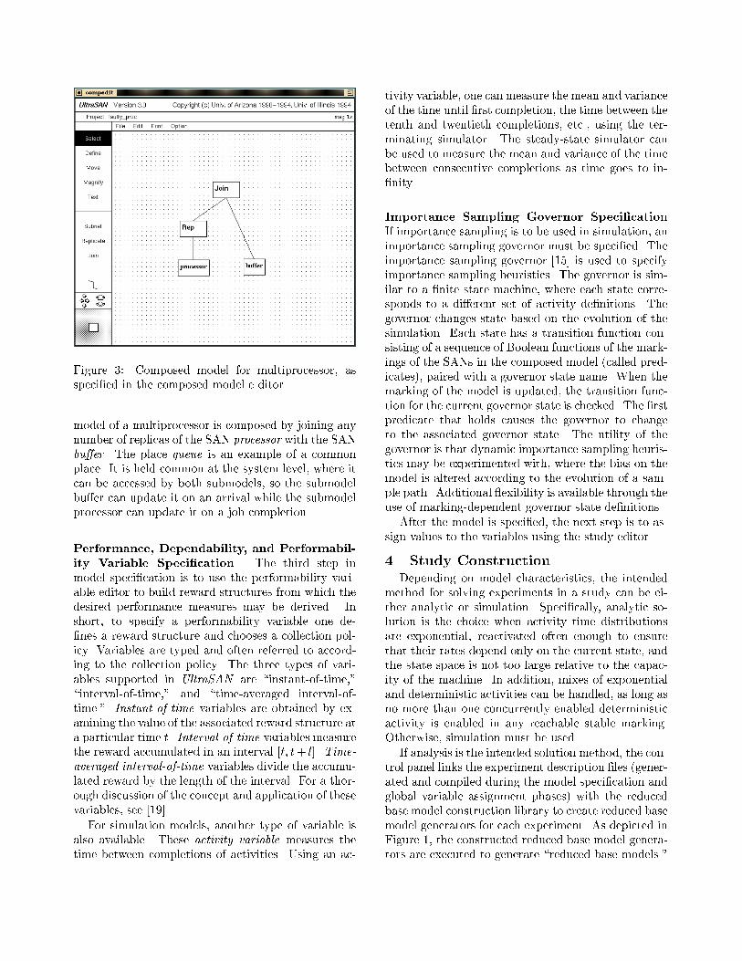
Figure 3: Composed model for multiprocessor, asspeci�ed in the composed model e ditor.

model of a multiprocessor is composed by joining anynumber of replicas of the SAN processor with the SANbu�er. The place queue is an example of a commonplace. It is held common at the system level, where itcan be accessed by both submodels, so the submodelbu�er can update it on an arrival while the submodelprocessor can update it on a job completion.

Performance, Dependability, and Performabil-

ity Variable Speci�cation The third step inmodel speci�cation is to use the performability vari-able editor to build reward structures from which thedesired performance measures may be derived. Inshort, to specify a performability variable one de-�nes a reward structure and chooses a collection pol-icy. Variables are typed and often referred to accord-ing to the collection policy. The three types of vari-ables supported in UltraSAN are \instant-of-time,"\interval-of-time," and \time-averaged interval-of-time." Instant-of-time variables are obtained by ex-amining the value of the associated reward structure ata particular time t. Interval-of-time variables measurethe reward accumulated in an interval [t; t+ l]. Time-

averaged interval-of-time variables divide the accumu-lated reward by the length of the interval. For a thor-ough discussion of the concept and application of thesevariables, see [19].

For simulation models, another type of variable isalso available. These activity variable measures thetime between completions of activities. Using an ac-

tivity variable, one can measure the mean and varianceof the time until �rst completion, the time between thetenth and twentieth completions, etc., using the ter-minating simulator. The steady-state simulator canbe used to measure the mean and variance of the timebetween consecutive completions as time goes to in-�nity.

Importance Sampling Governor Speci�cation

If importance sampling is to be used in simulation, animportance sampling governor must be speci�ed. Theimportance sampling governor [15] is used to specifyimportance sampling heuristics. The governor is sim-ilar to a �nite state machine, where each state corre-sponds to a di�erent set of activity de�nitions. Thegovernor changes state based on the evolution of thesimulation. Each state has a transition function con-sisting of a sequence of Boolean functions of the mark-ings of the SANs in the composed model (called pred-icates), paired with a governor state name. When themarking of the model is updated, the transition func-tion for the current governor state is checked. The �rstpredicate that holds causes the governor to changeto the associated governor state. The utility of thegovernor is that dynamic importance sampling heuris-tics may be experimented with, where the bias on themodel is altered according to the evolution of a sam-ple path. Additional exibility is available through theuse of marking-dependent governor state de�nitions.

After the model is speci�ed, the next step is to as-sign values to the variables using the study editor.

4 Study Construction

Depending on model characteristics, the intendedmethod for solving experiments in a study can be ei-ther analytic or simulation. Speci�cally, analytic so-lution is the choice when activity time distributionsare exponential, reactivated often enough to ensurethat their rates depend only on the current state, andthe state space is not too large relative to the capac-ity of the machine. In addition, mixes of exponentialand deterministic activities can be handled, as long asno more than one concurrently enabled deterministicactivity is enabled in any reachable stable marking.Otherwise, simulation must be used.

If analysis is the intended solution method, the con-trol panel links the experiment description �les (gener-ated and compiled during the model speci�cation andglobal variable assignment phases) with the reducedbase model construction library to create reduced basemodel generators for each experiment. As depicted inFigure 1, the constructed reduced base model genera-tors are executed to generate \reduced base models."

Each reduced base model is the state-level representa-tion of an experiment. The state-level representationconsists of a set of states, either a rate (if the transitionis caused by an exponential activity) or a probability(if the transition is caused by a deterministic activity)of transition between each pair of states, and a set ofimpulse and rate rewards for each state. (The impulsereward for a state is the impulse reward associatedwith the activity that completed to cause a transitionto the state.) The notion of state employed is variableand depends on the structure of the composed model.One can think of the state as a set of impulse andrate rewards plus a state tree [12], where each nodeon the state tree corresponds in type and level with anode on the composed model tree. Furthermore, eachnode in a state tree has associated with it a subset ofcommon places of the corresponding node in the com-posed model diagram. These places are those that arecommon at the node, but not at its parent node.

From a state, other states can be generated by ex-ecuting each activity that may complete in the state,generating a new state tree and impulse reward cor-responding to each possible next state that may bereached. For each possible next state, a non-zero rateor probability from the original state to the reachedstate is added to the list of rates to other states fromthe originating state. If the reached state is new, thenit is added to the list of states which need to be ex-panded. Generation of the reduced base model pro-ceeds by selecting states from the list of unexpandedstates and repeating the above operations. The proce-dure terminates when there are no more states to ex-pand. The resulting state-level representation servesas input to the analytic solvers, which determine theprobabilistic nature of the selected performability vari-ables.

If simulation is the intended solution method, thecontrol panel links experiments (model descriptions),with the simulation library to generate a simulationprogram. As depicted in Figure 1, two types of simu-lation programs can be generated: a steady state simu-

lator to solve long-run measures of performability vari-ables, and a terminating simulator to solve instant-of-time or interval-of-time performability variables.

Unlike the analytic solvers, which require a reducedbase model, the simulators execute directly on the as-signed model speci�cations. Both simulators exploitthe hierarchical structure and symmetries introducedby the replicate operation in a composed SAN-basedreward model to reduce the cost of future event listmanagement. More speci�cally, multiple future eventslists are employed, one corresponding to each leaf onthe state tree or, in other words, one corresponding to

each set of replica submodels in a particular marking.These multiple future event lists allow the simulatorsto operate on \compound events," corresponding to aset of enabled replica activities, rather than on indi-vidual activities. By operating on compound events,rather than individual activities, the number of checksthat must be made upon each activity completion isreduced. The details and precise algorithm can befound in [14]. This algorithm is the basis of the state-change mechanism for both steady-state and termi-nating simulators.

The next section details how the analytic and sim-ulation solvers are used to determine the probabilisticbehavior of the desired performability variables.

5 Study SolutionSolution of a set of base models, corresponding to

one or more experiments within a study, is the �nalstep in obtaining values for a set of performability vari-ables speci�ed for a model. The solution can be eitherby analytic (numerical) means or simulation, depend-ing on model characteristics and choices made in theconstruction phase of model processing. This sectiondetails the solution techniques employed in UltraSAN

to obtain analytic and simulative solutions.

5.1 Analytic Solution Techniques

Analytic solvers can provide steady-state as well astransient solutions for the reduced base model gen-erated during study construction. Figure 1 illus-trates the six solvers available for analytic solutions.Three of the solvers, speci�cally, the direct steady-statesolver, iterative steady-state solver, and deterministic

iterative steady-state solver provide steady-state so-lutions for the instant-of-time variables. The otherthree solvers, the transient instant-of-time solver,PDF interval-of-time solver and expected interval-of-

time solver, provide solutions for transient instant-of-time and interval-of-time variables. Except forthe two interval-of-time solvers, each solver calculatesthe mean, variance, probability density function, andprobability distribution function of the variable(s) it isintended to solve for. The PDF interval-of-time solvercalculates the probability distribution function of re-ward accumulated during a �xed interval of time [0; t].Likewise, the expected interval-of-time solver calcu-lates the expected reward accumulated during a �xedinterval of time. All solvers use a sparse matrix rep-resentation appropriate for the solution method em-ployed.

The direct steady-state solver uses LU decompo-sition [20] to obtain the steady-state solution forinstant-of-time variables. As with all steady-statesolvers, it is applicable when the generated reduced

base model is Markovian, and contains a single, irre-ducible, class of states. LU decomposition factors thetransition matrix Q into the product of a lower tri-angular matrix L and an upper triangular matrix U

such that Q = LU . Crout's algorithm [21] is incorpo-rated to compute L and U in a memory e�cient way.Pivoting in the solver is performed by using the im-proved generalized Markowitz strategy, as discussedby Osterby and Zlatev [22]. This strategy performspivoting on the element for which the minimum �ll-inis expected, subject to constraints on the magnitudeof the pivot. Furthermore, the matrix elements thatare less than some value (called the drop tolerance)are made zero (i.e., dropped) to retain the sparsity ofthe matrix during decomposition. In the end, itera-tive re�nement is used to correct the �nal solution toa user-speci�ed level of accuracy.

The iterative steady-state solver uses successive-overrelaxation to obtain steady-state instant-of-timesolutions. Like the direct steady-state solver, it actson the Markov process representation of a reducedbase model. However, being an iterative method, itavoids �ll-in problems inherent to the direct steady-state solver and therefore requires less memory. How-ever, unlike LU decomposition, SOR is not guaranteedto converge to the correct solution for all models. Inpractice however, this does not seem to be a prob-lem. The implementation solves the system of equa-tions directly, without �rst adding the constraint thatthe probabilities sum to one, and normalizes only atthe end, and as necessary to keep the solution vectorwithin bounds, as suggested in [23]. Selection of theacceleration factor is left to the user, and defaults toa value of 1 (resulting in a Gauss-Seidel iteration).

The deterministic iterative steady-state solver pro-vides a steady-state instant-of-time solution for mod-els that contain a mix of exponential and determin-istic timed activities. The method used in the solverwas �rst developed for deterministic stochastic Petrinets [24, 25] with one concurrently-enabled determin-istic transition and later adapted to SANs in whichthere is no more than one concurrently-enabled de-terministic activity [26]. In this solution method, aMarkov chain is generated for marking in which a de-terministic activity is enabled, representing the statesreachable from the current state due to completionsof exponential activities, until the deterministic activ-ity either completes or is aborted. The solver makesuse of successive-overrelaxation and uniformization toobtain the solution.

The transient instant-of-time solver and expectedinterval-of-time solver both use uniformization to ob-tain solutions. Uniformization works well when the

time point of interest is not too large, relative to thehighest rate activity in the model. The required Pois-son probabilities are calculated using the method byFox and Glynn [27] to avoid numerical di�culties.

The PDF interval-of-time solver [28] also uses uni-formization to calculate the probability distributionfunction of the total reward accumulated during a�xed interval [0; t]. This solver is unique among theexisting interval-of-time solvers in that it can solvefor reward variables containing both impulse and raterewards. The solver calculates the PDF of rewardaccumulated during an interval by conditioning onpossible numbers of transitions that may occur in aninterval, and possible sequences of state transitions(paths), given a certain number of transitions haveoccurred. Since the number of possible paths maybe very large, an implementation that considers allpossible paths would require a very large amount ofmemory. This problem is avoided in UltraSAN by cal-culating a bound on the error induced in the desiredmeasure by not considering each path, and discardingthose with acceptably small (user speci�ed) errors. Inmany cases, as illustrated in [28], selective discardingof paths can dramatically reduce the space requiredfor a solution while maintaining acceptable accuracy.Calculation of the PDF of reward accumulated, giventhat a particular path was taken, can also pose nu-merical di�culties. In this case, the solver makes se-lective use of multiprecision math to calculate severalsummations.

5.2 Simulative Solutions

As shown in Figure 1, three simulation-basedsolvers are available in UltraSAN. All three simula-tors exploit the hierarchical structure and symmetriesintroduced by the replicate operation in a composedSAN-based reward model to reduce the cost of futureevent list management. More speci�cally, multiple fu-ture events lists are employed, one corresponding toeach leaf on the state tree or, in other words, one cor-responding to each set of replica submodels in a partic-ular marking. These multiple future event lists allowthe simulators to operate on \compound events," cor-responding to a set of enabled replica activities, ratherthan on individual activities. By operating on com-pound events, rather than individual activities, thenumber of checks that must be made upon each activ-ity completion is reduced. The details and a precisealgorithm can be found in [14]. This algorithm is thebasis of the state-change mechanism for all three sim-ulators.

The steady-state simulator uses an iterative batchmeans method to estimate the means and/or variancesof steady-state instant-of-time variables. The user se-

lects a con�dence level and a maximum desired half-width for the con�dence interval corresponding to eachvariable, and the simulator executes batches until thecon�dence intervals for every performability variablesatisfy the user's criteria. The terminating simulationsolver estimates the means and/or variances for per-formability variables at a speci�c instant of time orover a given interval of time. It uses an iterative repli-cation method to generate con�dence intervals thatsatisfy the criteria speci�ed by the user.

The third simulation-based solver is a terminatingsimulator that is designed to use importance samplingto increase the e�ciency of simulation-based evalu-ation of rare event probabilities. The importancesampling terminating simulator estimates the meanof transient variables that are a�ected by rare eventsby simulating the model under the in uence of thegovernor (described in Section 3), so that the inter-esting event is no longer rare. The simulator thencompensates for the governor bias by weighting theobservations by the likelihood ratio. The likelihoodratio is calculated by evaluating the ratio of the like-lihood that a particular activity completes in a mark-ing, and that the completion of this activity resultsin a particular next marking, in the original model tothe likelihood of the same event in the governed model.The likelihood calculation is based on the work in [29],adapted for SAN simulation and implemented in Ul-

traSAN [15]. It works for models where all activitieshave closed-form activity time distribution functions.The probability distribution function is needed to han-dle the reactivations of activities when their de�nitionsare changed by the governor.

6 Conclusion

We have described version three of UltraSAN, asoftware package designed to facilitate the speci�-cation, construction, and solution of performabilitymodels represented as composed stochastic activitynetworks. Earlier versions of the package have been inuse for a period of about four years at several indus-trial and academic sites. Feedback from these users,and the development of new solution methods, hasmotivated the development of the new version of thesoftware. As described herein, version three embodiessigni�cant enhancements, relative to the earlier ver-sions, in both model solution capabilities and ease ofuse.

In particular, in the area of model speci�cation, theuser interface has been uni�ed under the control panel,which provides a simpler interface to the package thanin earlier versions, where the user was asked to run thevarious editors and solvers from the UNIX command

line. In addition, several new utilities are also avail-able from the control panel, including an automaticdocumentation facility. Furthermore, the generationand solution of large numbers of production runs fora model has been simpli�ed through the introductionof support for model speci�cations parameterized byglobal variables. A large part of the implementation ofsupport for parameterized models is the newly addedstudy editor, which expedites the assignment of val-ues to the global variables parameterizing the model.Finally, using the control panel, model constructionand solution can be distributed across a network ofworkstations and carried out in parallel.

In the area of model construction, support has beenadded to generate reduced base models for composedSANs that contain a mix of exponential and determin-istic timed activities. Three new solvers have also beenadded to UltraSAN. The �rst computes the probabil-ity distribution function of the reward accumulatedover an interval of time. The second computes theexpected value of transient interval-of-time variables.The third solver computes expected value, variance,probability density function, and probability distribu-tion function of steady-state instant-of-time variablesin SAN models with deterministic and exponential ac-tivities. Moreover, an importance sampling terminat-ing simulator has also been added to speed up thesimulation of systems with rare events.

These enhancements have resulted in a tool thatis easier to use, contains more model solution op-tions, and, as evidenced by its application (e.g.,[13, 30, 31, 32]), capable of evaluating the perfor-mance, dependability, and performability of realistic,real-world, systems. In addition to this capability, thetool serves as a test-bed in the development of newmodel construction and solution algorithms.

Acknowledgments

The success of this project is the result of the workof many people, in addition to the authors of this pa-per. In particular we would like to thank Burak Bu-lasaygun, Bruce McLeod, Aad van Moorsel, BhavanShah, and Adrian Suherman, for their contributions tothe tool itself, and the members of the PerformabilityModeling Research Lab who tested the pre-release ver-sions of the software. We would also like to thank theusers of the released versions who made suggestionsthat helped improve the software. In particular, wewould like to thank Steve West of IBM Corporation,Dave Krueger, Renee Langefels, and Tom Mihm ofMotorola Satellite Communications, Kin Chan, John

Chang, Ron Leighton and Kishore Patnam of US WestAdvanced Technologies, Lorenz Lercher of the Tech-nical University of Vienna, and John Meyer, of theUniversity of Michigan in this regard.

References[1] C. Lindemann, \DSPNexpress: A software package for

the e�cient solution of deterministic and stochastic Petri

nets," in Proceedings of the Sixth International Conference

on Modelling Techniques and Tools for Computer Systems

Performance Evaluation, (Edinburgh, Great Britain),

pp. 15{29, 1992.

[2] M. Bouissou, H. Bouhadana, M. Bannelier, and N. Vil-

latte, \Knowledge modeling and reliability processing: The

FIGARO language and associated tools," in Proceedings

of the Twenty-Third Annual International Symposium on

Fault-Tolerant Computing, (Toulouse, France), pp. 680{

685, June 1993.

[3] G. Chiola, \A software package for analysis of generalized

stochastic Petri net models," in Proceedings of the Inter-

national Workshop on Timed Petri Net Models, (Torino,

Italy), pp. 136{143, July 1985.

[4] W. H. Sanders and J. F. Meyer, \METASAN: A per-

formability evaluation tool based on stochastic activity net-

works," in Proceedings of the ACM-IEEE Computer Soci-

ety 1986 Fall Joint Computer Conference, pp. 807{816,

1986.

[5] G. Florin, P. Lonc, S. Natkin, and J. M. Toudic, \RDPS:

A software package for the validation and evaluation of de-

pendable computer systems," in Proceedings of the Fifth

IFAC Workshop Safety of Computer Control Systems

(SAFECOMP'86) (W. J. Quirk, ed.), (Pergamon, Sarlat,

France), pp. 165{170, October 1986.

[6] G. Ciardo, J. Muppala, and K. S. Trivedi, \SPNP: Stochas-

tic Petri net package," in Proceedings of the Fourth Inter-

national Workshop on Petri Nets and Performance Mod-

els, (Kyoto, Japan), pp. 142{151, December 1989.

[7] C. B�eounes, M. Agu�era, J. Arlat, S. Bachmann, C. Bour-

deau, J.-E. Doucet, K. Kanoun, J.-C. Laprie, S. Metge,

J. M. de Souza, D. Powell, and P. Spiesser, \SURF-2: A

program for dependability evaluation of complex hardware

and software systems," in Proceedings of the Twenty-Third

International Symposium on Fault-Tolerant Computing,

(Toulouse, France), pp. 668{673, June 1993.

[8] R. German, C. Kelling, A. Zimmermann, and G. Hommel,

\Timenet: A toolkit for evaluating non-markovian stochas-

tic petri-nets," tech. rep., Technische Universitat Berlin,

Germany, 1994. Submitted for publication.

[9] J. Couvillion, R. Freire, R. Johnson, W. D. Obal II, M. A.

Qureshi, M. Rai, W. H. Sanders, and J. Tvedt, \Performa-

bility modeling with UltraSAN," IEEE Software, vol. 8,

pp. 69{80, September 1991.

[10] M. Siegle, \Reduced Markov models of parallel programs

with replicated processes," in Proceedings of the Second

Euromicro Workshop on Parallel and Distri buted Pro-

cessing, (Malaga), pp. 1{8, January 1994.

[11] K. S. Trivedi, B. R. Haverkort, A. Rindos, and V. Mainkar,

\Techniques and tools for reliability and performance

evaluation: Proble ms and perspectives," in Computer

Performance Evaluation Modelling Tools and Techniques

(G. Haring and G. Kotsis, eds.), (New York), pp. 1{24,

Springer-Verlag, 1994.

[12] W. H. Sanders and J. F. Meyer, \Reduced base model con-

struction methods for stochastic activity networks," IEEE

Journal on Selected Areas in Communications, vol. 9,

pp. 25{36, January 1991.

[13] W. H. Sanders and L. M. Malhis, \Dependability evalua-

tion using composed SAN-based reward models," Journal

of Parallel and Distributed Computing, vol. 15, pp. 238{

254, July 1992.

[14] W. H. Sanders and R. S. Freire, \E�cient simulation of

hierarchical stochastic activity network models," Discrete

Event Dynamic Systems: Theory and Applications, vol. 3,

pp. 271{300, July 1993.

[15] W. D. Obal II and W. H. Sanders, \Importance sampling

simulation in UltraSAN," Simulation, vol. 62, pp. 98{111,

February 1994.

[16] W. D. Obal II and W. H. Sanders, \An environment for im-

portance sampling based on stochastic activity net works,"

in Proceedings of the 13th Symposium on Reliable Dis-

tributed Systems, (Dana Point, California), pp. 64{73, Oc-

tober 1994.

[17] Center for Reliable and High Performance Computing, Co-

ordinated Science Laboratory, University of Illinois, Ultra-

SAN Reference Manual, 1995.

[18] J. F. Meyer and W. H. Sanders, \Speci�cation and con-

struction of performability models," in Second Interna-

tional Workshop on Performability Modelling of Computer

and Communication Systems, (Le Mont Saint-Michel,

France), June 1993. Paper number 15.

[19] W. H. Sanders and J. F. Meyer, \A uni�ed approach for

specifying measures of performance, dependability, and

performability," in Dependable Computing for Critical Ap-

plications (A. Avizienis and J. C. Laprie, eds.), vol. 4 ofDe-

pendable Computing and Fault-Tolerant Systems, pp. 215{

238, Vienna: Springer Verlag, 1991.

[20] J. E. Tvedt, \Matrix representations and analytical solu-

tion methods for stochastic activity networks," Master's

thesis, The University of Arizona, 1990.

[21] W. H. Press, B. P. Flannery, S. A. Teukolsky, and W. T.

Vetterling, Numerical Recipes in C: The Art of Scienti�c

Computing. Cambridge University Press, 1988.

[22] O. Osterby and Z. Zlatev, Lecture Notes in Computer Sci-

ence: Direct Methods for Sparse Matrices. Heidelberg:

Springer-Verlag, 1983.

[23] U. R. Krieger, B. M�uller-Clostermann, and M. Sczittnick,

\Modeling and analysis of communication systems based

on computational m ethods for Markov chains," IEEE

Journal on Selected Areas in Communications, vol. 8,

no. 9, pp. 1630{1648, 1990.

[24] C. Lindemann, \An improved numerical algorithm for

calculating steady-state solutions of deterministic and

stochastic Petri net models," in Proceedings of the Fourth

International Workshop on Petri Nets and Performance

Models, (Melbourne, Australia), pp. 176{185, 1991.

[25] M. A. Marsan and G. Chiola, \On Petri nets with de-

terministic and exponentially distributed �ring times," in

Advances in Petri Nets 1986 (G. Rozenberg, ed.), Lecture

Notes in Computer Science 266, pp. 132{145, Springer,

1987.

[26] B. P. Shah, \Analytic solution of stochastic activity net-

works with exponential and deterministic activities," Mas-

ter's thesis, The University of Arizona, 1993.

[27] B. L. Fox and P. W. Glynn, \Computing Poisson probabil-

ities," Communications of the ACM, vol. 31, pp. 440{445,

1988.

[28] M. A. Qureshi and W. H. Sanders, \Reward model solution

methods with impulse and rate rewards: An algorit hm

and numerical results," Performance Evaluation, vol. 20,

pp. 413{436, August 1994.

[29] V. F. Nicola, M. K. Nakayama, P. Heidelberger, and

A. Goyal, \Fast simulation of dependability models with

general failure, repair and maintenance processes," in

Proceedings of the Twentieth Annual International Sym-

posium on Fault-Tolerant Computing, (Newcastle upon

Tyne, United Kingdom), pp. 491{498, June 1990.

[30] L. M. Malhis, W. H. Sanders, and R. D. Schlichting, \An-

alytic performability evaluation of a group-oriented multi-

cast protocol," Tech. Rep. PMRL 93-13, The University of

Arizona, June 1993. Submitted for publication.

[31] B. D. McLeod and W. H. Sanders, \Performance evalu-

ation of N-processor time warp using stochastic activity

networks," Tech. Rep. PMRL 93-7, The University of Ari-

zona, March 1993. Submitted for publication.

[32] W. H. Sanders, L. A. Kant, and A. Kudrimoti, \A modular

method for evaluating the performance of picture archiving

and communication systems," Journal of Digital Imaging,

vol. 6, pp. 172{193, August 1993.