MODEL SELECTION FOR REGULARIZED LEAST-SQUARESALGORITHM IN LEARNING THEORY

E. DE VITO, A. CAPONNETTO, AND L. ROSASCO

Abstract. We investigate the problem of model selection for learning algo-

rithms depending on a continuous parameter. We propose a model selectionprocedure based on a worst case analysis and data-independent choice of the

parameter. For regularized least-squares algorithm we bound the generaliza-

tion error of the solution by a quantity depending on few known constants andwe show that the corresponding model selection procedure reduces to solving a

bias-variance problem. Under suitable smoothness condition on the regression

function, we estimate the optimal parameter as function of the number of dataand we prove that this choice ensures consistency of the algorithm.

1. Introduction

A main goal of Learning Theory is the definition of an algorithm that, given a setof examples (xi, yi)`

i=1, returns a function f such that f(x) is an effective estimateof the output y when a new input x is given. The map f is chosen from a suitablespace of functions, called hypothesis space, encoding some a-priori knowledge onthe relation between x and y.

A learning algorithm is an inference process from a finite set of data based ona model represented by the hypothesis space. If the inference process is correctand the model realistic, as the number of available data increases, we expect thesolution to approximate the best possible solution. This property is usually calledconsistency, see [7], [8], [10], [12] and [21].

A central problem of Learning Theory is a quantitative assessment of the infer-ence property of a learning algorithm. A number of seminal works, see, for instance,[1], [7], [8] and [21], show that the essential feature of an algorithm should be thecapability of controlling the complexity of the solution. Roughly speaking, if themodel is too complex the algorithm solution overfits the data. In order to over-come overfitting, different complexity measures are introduced, as VC-dimension,see [21], Vγ-dimension, see [1], and covering numbers, see [7] and [24]. Interestingly,the good behavior of a large class of algorithms has been recently explained alsoin terms of stability with respect to variations of the given training set, see [4] and[17].

For both approaches it is natural to introduce a parametric family of learningalgorithms in which the parameters control the generalization properties. Typicalinstances of such algorithms are regularized (a la Tikhonov) algorithms, see, for

Date: October 5, 2004.

2000 Mathematics Subject Classification. Primary 68T05, 68P30.Key words and phrases. Model Selection, Optimal Choice of Parameters, Regularized Least-

Squares Algorithm.

Corresponding author: Ernesto De Vito, +390592055193 (phone), +39059370513 (fax).

1

2 E. DE VITO, A. CAPONNETTO, AND L. ROSASCO

instance, [6], [10], [11], [16] and [20]. In this context a central problem is theoptimal choice of the parameter as a function of the number of examples.

In this paper we address this issue for the learning algorithms arising in theminimization of the regularized empirical error

1`

∑i=1

(yi − f(xi))2 + λ ‖f‖2 ,

where the minimization takes place on a Hilbert space of continuous functions.The corresponding algorithm is usually called regularized least-squares algorithm orregularization networks, see [6], [10], [11] and [16].

In the above functional the first term measures the error of f on the givenexamples, while the second term is a penalty term that controls the “smoothness”of f in order to avoid overfitting. The parameter λ controls the trade-off betweenthese two terms, that is, the balance between the fitting capability of the solutionand its complexity.

Our results are in the spirit of [6] and [15]. In particular, our aim is to providea selection rule for the parameter λ which is optimal for any number ` of examplesand provides the desired asymptotic behavior when ` goes to infinity. As usual, see[7], [10] and [21], we describe the relation between x and y by means of an unknownprobability distribution ρ(x, y). Given a solution f , the expected risk∫

(y − f(x))2 dρ(x, y)

measures how well the probabilistic relation between x and y is described by thedeterministic rule y = f(x). Following [6], the optimal parameter is the one thatprovides the solution with minimal expectation risk. Since the expected risk isunknown, we need a probabilistic bound on it to have a feasible selection rule. Thebound we propose relies on the stability properties of the regularized least-squaresalgorithm, see [4], and does not depend on any complexity measure on H, which isa central tool in [6] and [15]. A different point of view is given in [20].

The paper is organized as follows. In Section 2 we recall some basic conceptof Learning Theory and we discuss the problem of model selection for algorithmsdepending on a parameter. In Section 3, we specialize this problem to the regu-larized least-squares algorithm and find a probabilistic bound for the expected riskof the solution, which is the main result of the paper. In Section 4 we estimatethe optimal parameter and prove the consistency of the regularized least-squaresalgorithm.

2. Learning Theory and optimal choice

This section is devoted to the following issues. First, we briefly recall the basicconcepts of Learning Theory. Second, we discuss the problem of the choice of theparameter for families of learning algorithms labeled by one real valued parameter.In particular, we give some insights into the relation between the Bayesian approach(average case) and the learning approach (worst case), and we propose a generalframework for parameter selection in a worst case scenario approach. Finally, wediscuss the problem of data dependent choice of the parameter. In the following weassume the reader to have a basic knowledge of Learning Theory (for reviews see[5], [7], [10], [12] and [21]).

MODEL SELECTION FOR RLS IN LEARNING THEORY 3

2.1. Learning Theory. In Learning Theory, examples are drawn from two sets:the input space X and the output space Y . The relation between the variable x ∈ Xand the variable y ∈ Y is not deterministic and it is described by a probability dis-tribution ρ, which is known only by means of ` examples D = ((x1, y1), . . . , (x`, y`)),drawn identically and independently from X × Y according to ρ. The set of ex-amples D is called training set. For regression problems, as we are dealing in thispaper, the output space Y is a subset of real numbers.

The aim of Learning Theory is to learn from a training set a function f : X → Y ,called estimator, such that f(x) is an effective estimate of y when x is given. Theinference property of f is measured by its expected risk

I[f ] =∫

X×Y

(f(x)− y)2 dρ(x, y).

Since we are dealing with regression problem, the choice of the quadratic loss func-tion is natural. However the discussion of this section holds for a wide class of lossfunctions (for a discussion of the properties of arbitrary loss function see [10], [18]and [20]).

In Learning Theory one approximates the probabilistic relation between x andy by means of functions y = f(x) defined on the input space X and belonging intosome a priori given set of model functions, called hypothesis space. For regressionproblems the model functions f are real valued.

A learning algorithm is a map that, given a training set D, outputs an estimatorfD chosen in the hypothesis space. A good algorithm is such that the expected riskI[fD] is as small as possible, at least for generic training sets.

A well known example of learning algorithm is the empirical risk minimizationalgorithm, see, for instance, [7], [10] and [21]. For a training set D, the estimatorfD is defined as the one that minimizes the empirical risk

IDemp[fD] =

1`

∑i=1

(fD(xi)− yi)2

over the hypothesis space. Different choices of the hypothesis space give rise todifferent algorithms, so one usually introduces a sequence of nested hypothesisspaces

Hλ1 ⊂ Hλn ⊂ . . . ⊂ H,

where λ1 > λ2 > . . . λn andHλkis the subset of functions in the model spaceH that

have complexity less than 1λk

, according to some suitable measure on complexity(for example the inverse of the norm of f , see [7], or its VC-dimension, see [10]and [21]). The regularized least-squares algorithm discussed in the introduction isanother example of a learning algorithm: for a training set D, the estimator fD isdefined as the minimizer of

1`

∑i=1

(yi − f(xi))2 + λ ‖f‖2 ,

where the minimum is on a Hilbert space H of functions defined on X (other lossfunctions and penalty terms can be considered instead of ‖f‖2, see [10], [20] and[21] for a discussion).

In both examples there is a family of algorithms labeled by a parameter control-ling the complexity of the estimator. The problem of model selection corresponds

4 E. DE VITO, A. CAPONNETTO, AND L. ROSASCO

to characterizing a rule for the choice of the parameter in such a way that somecriterion of optimality with respect to the inference and consistency properties issatisfied. The following section discusses this question.

2.2. Optimal choice and model selection rule. In the following we consider afamily of learning algorithms that are labeled by a positive parameter λ; we assumethat the complexity of the solution decreases with λ. Given a parameter λ and atraining set D, the algorithm provides an estimator fλ

D ∈ H, where H is somegiven (vector) space of functions. In this paper the space H is given, however onecan easily extend the present discussion to the case of H being labeled by someparameters, as kernel parameters when H is a reproducing kernel Hilbert space, see[2].

In this framework the problem of model selection is the problem of the choice ofthe optimal parameter λ. In applications the parameter λ is usually chosen throughan a posteriori procedure like cross-validation or using a validation set, see, forinstance, [22].

To give an a priori definition of the optimal regularization parameter we recallthat a good estimator fλ

D should have small expected risk I[fλD]. So a natural defi-

nition for the optimal parameter λopt, is the value of λ minimizing I[fλD]. However,

this statement needs some careful examination since I[fλD] is a random variable

on the sample space of all training sets. This observation introduces some degreeof freedom in the definition of λopt. Following a Bayesian approach, a possibledefinition is the following one

(1) λopt := argminλ>0

ED(I[fλD]),

where ED denotes the expectation with respect to the training sets, see [23]. Theabove definition can be refined by considering also the variance σ2 of the randomvariable, for example considering

(2) λopt := argminλ>0

{ED(I[fλD]) + σ2(I[fλ

D])}.

A third possibility is the worst case analysis. Given a confidence level η ∈ (0, 1)and defined the quantity

Eopt(λ, η) := inft∈[0;+∞)

{ t | Prob{D ∈ Z` | I[fλD] > t} ≤ η},

one lets the optimal parameter be

(3) λopt(η) := argminλ>0

Eopt(λ, η).

We notice that the first two definitions require the knowledge of the first (andsecond) order momentum of the random variable I[fλ

D]. This is a satisfactorycharacterization if we assume to deal with normal distributions. On the other handit is easy to see that the third definition amounts to a complete knowledge of therandom variable I[fλ

D]. Indeed, given λ, Eopt(λ, η), viewed as function of 1 − η, isthe inverse of the distribution function of I[fλ

D].However, in Learning Theory, the above definitions have only a theoretical mean-

ing since the distribution ρ and, hence, the random variable I[fλD] are unknown.

To overcome this problem, one studies the random variable I[fλD] through a known

MODEL SELECTION FOR RLS IN LEARNING THEORY 5

probabilistic bound E(λ, `, η) of the form

(4) Prob{D ∈ Z` | I[fλD] > E(λ, `, η)} ≤ η.

For the worst case setting the above expression leads to the following model selectionrule

(5) λ0(`, η) := argminλ>0

E(λ, `, η).

In order to make the above definition rigorous we assume that E extends to acontinuous function of λ on [0,+∞] into itself, and replace (5) by

(6) λ0(`, η) = max argminλ∈[0,+∞]

E(λ, `, η).

The continuity of E ensures that the definition is well stated, even if λ0 could beoccasionally zero or infinite. We select the maximum among the minimizers of Eto enforce uniqueness of λ0: this choice appears quite natural since it correspondsto the most regular estimator fitting the constraint of minimizing the bound.

Some remarks are in order. First of all, different bounds E give rise to differentselection criteria. Moreover to have a meaningful selection rule the bound E hasto be a function only of known quantities. In this paper we exhibit a bound thatgives rise to an optimal parameter defined through a simple algebraic equation.Second, the random variable I[fλ

D] depends on the number ` of examples in thetraining set and, as a consequence, the optimal parameter λ0 is a function of `. Soit is natural to study the asymptotic properties of our selection rule when ` goesto infinity. In particular, a basic requirement is consistency, that is, the fact thatI[fλ0(`)

D ] tends to the smallest attainable expected risk as the number of data goesto infinity. The concept of (weak universal) consistency is formally expressed bythe following definition, see [8],

Definition 1. The one parameter family of estimators fλD provided with a model

selection rule λ0(`) is said to be consistent if, for every ε > 0, it holds

lim`→∞

supρ

Prob{D ∈ Z` | I[fλ0(`)D ] > inf

f∈HI[f ] + ε} = 0,

where the sup is over the set of all probability measures on X × Y .

In the above definition, the number inff∈H I[f ] represents a sort of bias error,[12], associated with the choice of H and, hence, it can not be controlled by theparameter λ. In particular if there exists fH ∈ H such that I[fH] = inff∈H I[f ], theestimator fH is the best possible deterministic description we can give of the relationbetween x and y, for given H. For sake of clarity, we notice that, for empirical riskminimization algorithm, the bias error is usually called approximation error and itis controlled by the choice of the hypothesis space, see [7] and [15].

2.3. Data dependency. The choices of the parameter λ discussed in the abovesection are a priori since do not depend on the training set D. One could alsoconsider a posteriori choices where λ0 depends on the training set D. In a worstcase analysis, this corresponds to considering a bound depending explicitly on D,that is

(7) Prob{D ∈ Z` | I[fλD] > E(λ, `, η, D)} ≤ η.

6 E. DE VITO, A. CAPONNETTO, AND L. ROSASCO

A well-known example of the above bound is the principle of structural risk min-imization, see [10] and [21]. For Empirical Risk Minimization algorithm in nestedhypothesis spaces

Hλ1 ⊂ Hλn⊂ . . . ⊂ H,

the parameter λ is chosen in order to minimize the bound

(8) E(λ, `, η, D) = IDemp[f

λD] + G(λ, `, η, D),

where G(λ, `, η, D) is a term that controls the complexity of the solution. Usually, Gdoes not dependent on the training set since the measure of complexity is uniformon the hypothesis space Hλ. However, we get a dependence of the bound on Dbecause of the presence of the empirical term ID

emp[fλD] in Eq. (8).

Now, mimicking the idea of previous discussion, we could define the optimalparameter as

λ0(`, η,D) := argminλ>0

E(λ, `, η, D).

Clearly, we get a dependence of the optimal parameter on the training set D. Thisdependence can be, in principle, problematic due to the probabilistic nature ofEq. (4). Indeed, for every λ, we can define the collection of good training sets forwhich the bound is tight, i.e.

A(λ) = {D ∈ Z` | I[fλD] ≤ E(λ, `, η, D)}.

By definition of the bound E, the probability of drawing a good training set D ∈A(λ) is greater than 1−η. However, the previous confidence level cannot be appliedto I[fλ0(D)

D ]. Indeed, it can happen that the probability of drawing a training setD in the set

{D ∈ Z` | I[fλ0(D)D ] ≤ E(λ0(D), `, η,D)} = {D ∈ Z` | D ∈ A(λ0(D))}

could be much smaller that 1 − η, depending on the structure of the sets A(λ) inthe sample space Z`. Simple toy examples of this pathology can be built.

A possible solution to this kind of problem requires further analyses, see, forinstance, [3], [8] and [21]. In this paper we avoid the problem by considering dataindependent bounds and hence a priori model selection rules.

3. A probabilistic bound for regularized least-squares algorithm

We consider throughout the problem of model selection for regularized least-squares algorithm in the regression setting.

In the present section we first show that the expected risk of the estimator fλD

concentrates around the expected risk of fλ, where fλ is the minimizer of theregularized expected risk I[f ] + λ ‖f‖2H.

Moreover, we give a probabilistic bound of the difference between I[fλD] and

I[fλ] in terms of a function S(λ, `, η) depending on the parameter λ, the numberof examples ` and the confidence level 1 − η. Our results are based on stabilityproperties of regularized least-squares algorithm, see [4], and the McDiarmid con-centration inequality, see [13]. In particular, we do not make use of any complexitymeasure on the hypothesis space, like VC-dimension, see [21], or covering number,see [7] and [15]. We stress that the bound S depends on H only through two simpleconstants related to topological properties of X and Y .

Compared to previous results (see, for instance, [3], [4], [7], [14], [15], [21]) weare not interested into the deviation of the empirical risk from the expected risk

MODEL SELECTION FOR RLS IN LEARNING THEORY 7

and we bound directly the expected risk of the estimator fλD. Moreover, our result

concentrates I[fλD] around I[fλ] both from above and below so that I[fλ] will

play the role of approximation error and S(λ, `, η) the role of sample error (ourterminology is close to the definition of [6], which is somewhat different with thenotation of [7] and [15]).

Finally, in order to obtain algorithmically computable results, we make somesmoothness assumption on the probability distribution ρ. By means of standardresults in approximation theory, see [19], we find a bound E, depending only onknown quantities.

Before stating the main theorem of the section we set the notations.

3.1. Notations. We assume that the input space X is a compact subset of Rd andthe output space Y is a compact subset of R. The assumption of compactness isfor technical reasons and simplifies some proof.

We let ρ be the unknown probability measure on Z = X × Y describing therelation between x ∈ X and y ∈ Y , and ν the marginal distribution of ρ on X.Moreover, for ν-almost all x ∈ X, let ρx be the conditional distribution of y withrespect to x.

If ξ is a random variable on Z, we denote its mean value by EZ (ξ),

EZ (ξ) =∫

X×Y

ξ(x, y) dρ(x, y).

As usual, L2(X, ν) is the Hilbert space of square-integrable functions and ‖·‖ν ,〈·, ·〉ν are the corresponding norm and scalar product.

We let C(X) be the space of (real) continuous functions on X equipped with theuniform norm, ‖f‖∞ = supx∈X |f(x)|.

We denote by f0 and σ0 the regression and noise functions defined respectivelyas

f0(x) =∫

Y

y dρx(y),(9)

σ20(x) =

(∫Y

y2 dρx(y))− (f0(x))2 ,(10)

that belong to L2(X, ν) due to the compactness of X and Y .Given ` ∈ N, let Z` be the set of all training sets with ` examples. We regard

Z` as a probability space with respect to the product measure ρ` = ρ⊗ . . .⊗ ρ. Ifξ is a random variable on Z` we denote its mean value by ED (ξ),

ED (ξ) =∫

Z`

ξ(D) dρ`(D).

Given D ∈ Z`, let ρD be the empirical measure on X × Y defined by D, that is

ρD =1`

∑i=1

δxiδyi

,

where δx and δy are the Dirac measures at x and y respectively.We assume the hypothesis space H be a reproducing kernel Hilbert space with a

continuous kernel K : X×X → R. The assumption on the kernel ensures H being a

8 E. DE VITO, A. CAPONNETTO, AND L. ROSASCO

Hilbert space of continuous functions. We let ‖·‖H and 〈·, ·〉H be the correspondingnorm and scalar product. We define

Kx(s) = K(s, x) x ∈ X

κ = sup{√

K(x, x) |x ∈ X},(11)δ = sup{|y| | y ∈ Y }.(12)

It is well known, see [2] and [7], that

H ⊂ C(X) ⊂ L2(X, ν),f(x) = 〈f,Kx〉H , x ∈ X

‖·‖ν ≤ ‖·‖∞ ≤ κ ‖·‖H .(13)

We denote by Lν the integral operator on L2(X, ν) with kernel K, that is,

(14) (Lνf)(s) =∫

X

K(s, x)f(x)dν(x) s ∈ X,

and by P the projection onto the closure of the range of Lν . In particular, one hasthat the closure of H with respect the norm of L2(X, ν) is PL2(X, ν).

We recall that, given f ∈ L2(X, ν), the expected risk of f is

I[f ] =∫

X×Y

(y − f(x))2 dρ(x, y).

We let IH be the bias error

IH = inff∈H

I[f ],

For any λ > 0 we denote by fλ the solution of

minf∈H

{I[f ] + λ ‖f‖2H},(15)

which exists and it is unique, see, for instance, [6].Finally, given D ∈ Z`, the empirical risk of f ∈ C(X) is given by

IDemp[f ] =

1`

∑i=1

(yi − f(xi))2.

For all λ > 0, the estimator fλD is defined as the unique solution of

(16) minf∈H

{IDemp[f ] + λ ‖f‖2H},

which exists and it is unique, see [6].In the following we will always consider the square root of the unbiased risk that

we indicate with R[f ] to simplify the notation, that is

R[f ] =√

I[f ]− IH.

Indeed, Eq. (21) below will show that this quantity can conveniently be interpretedas a distance in L2(X, ν).

MODEL SELECTION FOR RLS IN LEARNING THEORY 9

3.2. Main results. The following theorem shows that, given the parameter λ,the expected risk of the estimator fλ

D provided by the regularized least-squaresalgorithm concentrates around the value I[fλ]. Moreover, the deviation can bebounded by a simple function S depending only on the confidence level, the numberof examples and two constants, κ and δ, encoding some topological properties ofX, Y and the kernel (see Eqs. (11) and (12)).

Theorem 1. Given 0 < η < 1, ` ∈ N and λ > 0, with probability at least 1− η,∣∣R[fλD]−R[fλ]

∣∣ ≤ S(λ, `, η),

where

(17) S(λ, `, η) =δ κ2

λ√

`

(1 +

κ√λ

)(1 +

√2 log

2η

).

The proof of the theorem is postponed to Section 3.3 after a brief discussion andsome remarks on the result.

Let us interpret the quantities occurring in our inequality. The data indepen-dent term R[fλ] can be interpreted as the price payed by replacing the regressionfunction f0 with the regularized solution fλ, in short as the approximation error,compare with [6] and [15].The term S(λ, `, η) is a bound on

∣∣R[fλD]−R[fλ]

∣∣, that is on the sample errormade by approximating fλ through a finite training set D, compare with [6], [15]and [21].

Since Theorem 1 bounds R[fλD] both from above and below and S(λ, `, η) goes to

zero for ` going to +∞, the expected risk of fλD concentrates around the expected

risk of fλ. Then the splitting of R[fλD] into approximation error and sample error

appears quite natural and intrinsic to the problem.

3.3. Proofs. In the following, before dealing with the main result, we briefly sketchthe scheme of the proof and we show some useful lemmas.The proof of Theorem 1 is essentially based on two steps

• we show that regularized least-squares algorithm satisfies a kind of stabilityproperty with respect to variation of the training set, compare with [4];

• we give an estimate of the mean value of R[fλD] (and hence of the mean

value of the expected risk).

More precisely, given λ, we regard R[fλD] as a real random variable on Z` and we

apply the McDiarmid inequality, see [13]. This inequality tells us that

(18) Prob{D ∈ Z` | |R[fλD]− ED

(R[fλ

D])| ≥ ε} ≤ 2e

− 2ε2∑`i=1 c2

i

provided that

(19) supD∈Z`

sup(x′,y′)∈Z

|R[fλD]−R[fλ

Di ] | ≤ ci

where Di is the training set with the ith example being replaced by (x′, y′).

10 E. DE VITO, A. CAPONNETTO, AND L. ROSASCO

To work out the proof, we recall some preliminary facts. Since we are consideringthe quadratic loss the expected risk of f ∈ H can be written in the following way,

I[f ] = ‖f − f0‖2ν + ‖σ0‖2ν(20)

= ‖P (f − f0)‖2ν + ‖(I − P )(f − f0)‖2ν + ‖σ0‖2ν= ‖f − Pf0‖2ν + ‖(I − P )(f − f0)‖2ν + ‖σ0‖2ν= ‖f − Pf0‖2ν + ‖(I − P )f0‖2ν + ‖σ0‖2ν

where f0 and σ0 are given by Eqs. (9) and (10), and (I − P )f = 0 since f ∈ H ⊂PL2(X, ν).It follows that IH = inff∈H I[f ] = ‖(I − P )f0‖2ν + ‖σ0‖2ν and

(21) R[f ] =√

I[f ]− IH = ‖f − Pf0‖ν .

We now recall the explicit form of the minimizers of (15) and (16). One has that

fλ = (T + λ)−1gρ(22)

fλD = (Tx + λ)−1gD(23)

where T and Tx are positive operators on H given by

T =∫

X

〈·,Kx〉HKx dν(x)(24)

Tx =1`

∑i=1

〈·,Kxi〉H Kxi(25)

and gρ and gD are functions in H defined by

gρ =∫

X

Kx f0(x) dν(x)(26)

gD =1`

∑i=1

yiKxi ,(27)

(in Eq. (24) the integral is taken with respect to the trace operator norm, whilein Eq. (26) the integral is with respect to the norm of H. Both integrals are finitesince the integrands are continuous and X is compact).

In order to present the proof of Theorem 1 we need some preliminary Lemmas.The first one provides an upper bound on

∥∥fλD

∥∥H. The proof is standard and we

report it for completeness, see, for instance, [4].

Lemma 1. For all λ > 0, ∥∥fλD

∥∥H ≤ δ√

λ.

Proof. Since by definition, see Eq. (16),

fλD = argmin

f∈H{ID

emp[f ] + λ ‖f‖2H},

with the choice f = 0, it follows that

IDemp[f

λD] + λ

∥∥fλD

∥∥2

H ≤ IDemp[0] + λ ‖0‖2H =

1`

∑i=1

y2i ≤ δ2,

MODEL SELECTION FOR RLS IN LEARNING THEORY 11

where in the last inequality we recalled the definition of δ, see Eq. (12). The thesisfollows from the fact that ID

emp[fλD] ≥ 0. �

The next step is the estimate of the expectation value of ‖Tx − T‖ (here ‖·‖denotes the operator norm in H) and that of ‖gD − gρ‖H. To this aim, we recallthe following property regarding vector valued random variables on Z. Let K be aHilbert space and ξ a K-valued random variable on Z, then

ED

(∥∥∥∥∥1`

∑i=1

ξ(xi, yi)− EZ (ξ)

∥∥∥∥∥K

)2

≤ ED

∥∥∥∥∥1`

∑i=1

ξ(xi, yi)− EZ (ξ)

∥∥∥∥∥2

K

=

1`

(EZ

(‖ξ‖2K

)− ‖EZ (ξ)‖2K

).(28)

The first inequality is consequence of Schwarz inequality and the equality is astraightforward extension of the well-known property of real random variables, see[9].

Lemma 2. Let a1 =∫

X×X

(K(x, x)2 −K(x, x′)2

)dν(x)dν(x′), then

ED (‖Tx − T‖) ≤√

a1

`

≤ κ2

√`.

Proof. Let B2(H) be the Hilbert space of selfadjoint Hilbert-Schmidt operators onH with scalar product 〈A,B〉B2(H) = Tr (AB). Notice that, for all x ∈ X, the rankone operator 〈·,Kx〉HKx is in B2(H), so we can define the B2(H)-valued randomvariable ξ as

ξ(x) = 〈·,Kx〉HKx.

Since Tr (〈·,Kx〉HKx′) = 〈Kx′ ,Kx〉H then

‖ξ(x)− ξ(x′)‖2B2(H) = Tr ((ξ(x)− ξ(x′))2)

= K2(x, x) + K2(x′, x′)− 2K2(x′, x),

which implies the continuity of ξ. Its mean value is given by

EZ (ξ) =∫

X

〈·,Kx〉HKx dν(x)

= T.

Now, observe that

ED

(‖ξ‖2B2(H)

)= ED (Tr (〈·,Kx〉HKxK(x, x)))

=∫

X

K(x, x)2 dν(x)

Finally,

‖EZ (ξ)‖2B2(H) = Tr (T 2)

=∫

X×X

Tr (〈·,Kx〉HKx′K(x, x′)) dν(x)dν(x′)

=∫

X×X

K(x, x′)2 dν(x)dν(x′).

12 E. DE VITO, A. CAPONNETTO, AND L. ROSASCO

Applying Eq. (28) and the definition of a1, one has that

ED

(‖Tx − T‖B2(H)

)≤√

a1

`

The thesis follows observing that

‖Tx − T‖ ≤ ‖Tx − T‖B2(H)

and

a1 ≤∫

X

K(x, x)2 dν(x) ≤ κ4.

�

Lemma 3. Let a2 =∫

Zy2K(x, x)dρ(x, y)− ‖gρ‖2H, then

ED

(‖gD − gρ‖H

)≤

√a2

`

≤ δ κ√`.

Proof. We follow the scheme of the previous proof. Let ξ be the H-valued randomvariable

ξ(x, y) = yKx.

Since

‖ξ(x, y)− ξ(x′, y′)‖2H = y2K(x, x) + y′2K(x′, x′)− 2yy′K(x, x′)

ξ is continuous and

EZ (ξ) =∫

X×Y

yKx dρ(x, y)

= gρ,

by definition of gρ.Moreover

EZ

(‖ξ‖2H

)=

∫X×Y

y2K(x, x) dρ(x, y).

Applying Eq. (28) and the definition of a2, one has that

ED

(‖gD − gρ‖H

)≤ a2

`.

The thesis follows observing that

0 ≤ a2 ≤∫

X×Y

y2K(x, x) dρ(x, y) ≤ δ2 κ2.

�

The next lemma estimates the expectation value of R[fλD].

Lemma 4. Following the above notations∣∣ED

(R[fλ

D])−R[fλ]

∣∣ ≤ κ2δ

λ√

`

(1 +

κ√λ

).

MODEL SELECTION FOR RLS IN LEARNING THEORY 13

Proof. By means of Eq. (23),

fλD = (Tx + λ)−1gD

= (T + λ)−1 (gD − gρ)

+ (T + λ)−1(T − Tx)(Tx + λ)−1gD

+ (T + λ)−1gρ,

that is, using Eq. (22),

fλD − fλ = (T + λ)−1 (gD − gρ) + (T + λ)−1(T − Tx)fλ

D.

Using Eq. (21) and the triangular inequality we have that∣∣R[fλD]−R[fλ]

∣∣ ≤∥∥fλ

D − fλ∥∥

ν

( Eq. (13) ) ≤ κ∥∥(T + λ)−1(gD − gρ)

∥∥H

+ κ∥∥(T + λ)−1(T − Tx)fλ

D

∥∥H

≤ κ

λ‖gD − gρ‖H +

κδ

λ32‖T − Tx‖ ,

where∥∥(T + λ)−1

∥∥ ≤ 1λ and we used Lemma 1 to bound

∥∥fλD

∥∥H.

Finally we take the mean value on D and use Lemmas 2 and 3. �

We are now ready to prove the main result of the Section.

Proof of Theorem 1. The proof uses the McDiarmid inequality (18). Due to Eq. (21),the conditions (19) become

supD∈Z`

sup(x′,y′)∈Z

|∥∥fλ

D − Pf0

∥∥ν−∥∥fλ

Di − Pf0

∥∥ν| ≤ ci

(we recall that Di is the training set where the ith example is replaced by (x′, y′)).In order to compute the constants ci, we notice that fλ

D can be decomposed, bymeans of Eq. (23), as

fλD = (Tx + λ)−1gD

= (Tx + λ)−1 (gD − gDi)+ (Tx + λ)−1(Txi − Tx)(Txi + λ)−1gDi

+ (Txi + λ)−1gDi ,

that is, using again Eq. (23) with Di,

fλD − fλ

Di = (Tx + λ)−1 (gD − gDi) + (Tx + λ)−1(Txi − Tx)fλDi .

By the triangular inequality, we can write

|∥∥fλ

D − Pf0

∥∥ν−∥∥fλ

Di − Pf0

∥∥ν| ≤

∥∥fλD − fλ

Di

∥∥ν

( Eq. (13) ) ≤ κ∥∥(Tx + λ)−1(gD − gDi)

∥∥H

+ κ∥∥(Tx + λ)−1(Tx − Txi)fλ

Di

∥∥H

≤ 2δ κ2

λ`

(1 +

κ√λ

)=: ci

14 E. DE VITO, A. CAPONNETTO, AND L. ROSASCO

where we used Lemma 1 to bound∥∥fλ

Di

∥∥H and∥∥(Tx + λ)−1

∥∥ ≤ 1λ

,

‖Tx − Txi‖ =1`

∥∥∥〈·,Kxi〉HKxi −⟨·,Kx′i

⟩HKx′i

∥∥∥≤ 1

`2 κ2,

‖gD − gDi‖H =1`

∥∥yKxi − y′iKx′i

∥∥H

≤ 1`2δ κ.

Plugging the constants ci into McDiarmid inequality (18), we have that∣∣R[fλD]− ED

(R[fλ

D])∣∣ ≤ ε

with probability

1− 2e

− ε2

2(

δ κ2λ√

`

(1+ κ√

λ

))2

= 1− η

so, with probability at least 1− η,∣∣R[fλD]− ED

(R[fλ

D])∣∣ ≤ δ κ2

λ√

`

(1 +

κ√λ

)√2 log

2η.

The above bound together with Lemma 4, once again by the triangular inequality,completes the proof. �

4. Estimate of the optimal parameter

We are now in the position to apply the results of the previous Section to theactual estimate of the regularization parameter, following the technique presentedin Section 2.

From Theorem 1 we can easily derive the following bound

(29) R[fλD] ≤ R[fλ] + S(λ, `, η),

which holds with probability at least 1− η.From the explicit form of S(λ, `, η), we have that S(λ, `, η) decreases with λ and

goes to +∞ when λ goes to 0. On the other hand, it is easy to check that R[fλ] isan increasing function of λ and goes to 0 for λ going to 0, see [6].

The bound (29) is of the form of Eq. (4) and can be used in the model selectionrule defined by Eq. (6). Our definition ensures existence and uniqueness of theestimate λ0 of the optimal parameter, however we still have to prove that λ0 isfinite. We now prove that the bound in Eq. (29) provides an estimate λ0 that isfinite for large enough `.

We consider a slightly more general case that will be useful in the following. Welet A(λ) be an upper bound on the approximation error, that is, an increasing,continuous function from [0,+∞] to [0,+∞] satisfying

A(λ) ≥ R[fλ],

andlimλ→0

A(λ) = 0.

MODEL SELECTION FOR RLS IN LEARNING THEORY 15

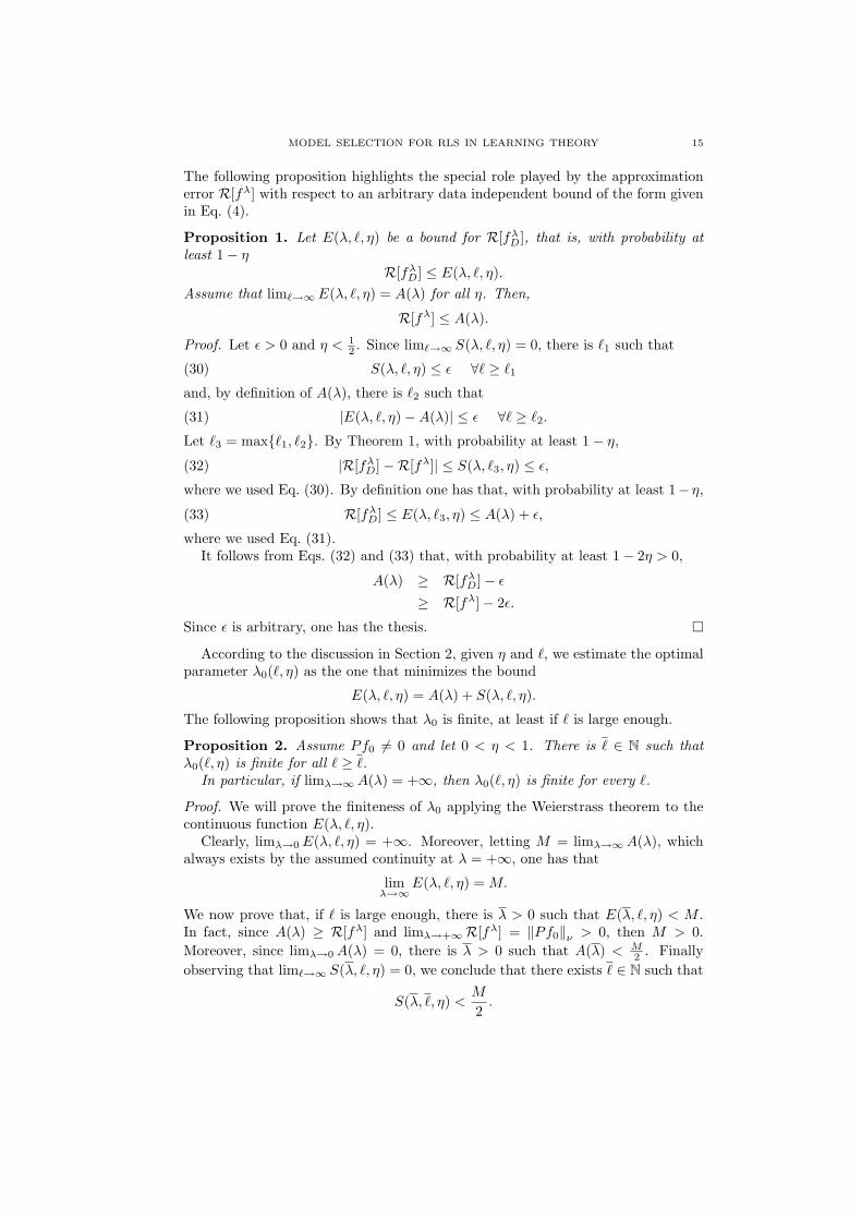
The following proposition highlights the special role played by the approximationerror R[fλ] with respect to an arbitrary data independent bound of the form givenin Eq. (4).

Proposition 1. Let E(λ, `, η) be a bound for R[fλD], that is, with probability at

least 1− ηR[fλ

D] ≤ E(λ, `, η).Assume that lim`→∞E(λ, `, η) = A(λ) for all η. Then,

R[fλ] ≤ A(λ).

Proof. Let ε > 0 and η < 12 . Since lim`→∞ S(λ, `, η) = 0, there is `1 such that

(30) S(λ, `, η) ≤ ε ∀` ≥ `1

and, by definition of A(λ), there is `2 such that

(31) |E(λ, `, η)−A(λ)| ≤ ε ∀` ≥ `2.

Let `3 = max{`1, `2}. By Theorem 1, with probability at least 1− η,

(32) |R[fλD]−R[fλ]| ≤ S(λ, `3, η) ≤ ε,

where we used Eq. (30). By definition one has that, with probability at least 1− η,

(33) R[fλD] ≤ E(λ, `3, η) ≤ A(λ) + ε,

where we used Eq. (31).It follows from Eqs. (32) and (33) that, with probability at least 1− 2η > 0,

A(λ) ≥ R[fλD]− ε

≥ R[fλ]− 2ε.

Since ε is arbitrary, one has the thesis. �

According to the discussion in Section 2, given η and `, we estimate the optimalparameter λ0(`, η) as the one that minimizes the bound

E(λ, `, η) = A(λ) + S(λ, `, η).

The following proposition shows that λ0 is finite, at least if ` is large enough.

Proposition 2. Assume Pf0 6= 0 and let 0 < η < 1. There is ` ∈ N such thatλ0(`, η) is finite for all ` ≥ `.

In particular, if limλ→∞A(λ) = +∞, then λ0(`, η) is finite for every `.

Proof. We will prove the finiteness of λ0 applying the Weierstrass theorem to thecontinuous function E(λ, `, η).

Clearly, limλ→0 E(λ, `, η) = +∞. Moreover, letting M = limλ→∞A(λ), whichalways exists by the assumed continuity at λ = +∞, one has that

limλ→∞

E(λ, `, η) = M.

We now prove that, if ` is large enough, there is λ > 0 such that E(λ, `, η) < M .In fact, since A(λ) ≥ R[fλ] and limλ→+∞R[fλ] = ‖Pf0‖ν > 0, then M > 0.Moreover, since limλ→0 A(λ) = 0, there is λ > 0 such that A(λ) < M

2 . Finallyobserving that lim`→∞ S(λ, `, η) = 0, we conclude that there exists ` ∈ N such that

S(λ, `, η) <M

2.

16 E. DE VITO, A. CAPONNETTO, AND L. ROSASCO

It follows that, since S is a decreasing function of `, for all ` ≥ `,

E(λ, `, η) ≤ E(λ, `, η) < M.

Hence, by means of Weierstrass theorem E(λ, `, η) attains its minimum. Moreover,minE ≤ E(λ, `, η) < M so that all the minimizers are finite.

Assume now that limλ→∞A(λ) = +∞, then M = +∞ and, clearly, minE <+∞, so that the minimizers are finite for all `. �

Remark 1. The assumption that Pf0 6= 0 is natural. If Pf0 = 0, the problem ofmodel selection is trivial since H is too poor to give a reasonable approximation off0 still with infinite data.

In order to actually use the estimate λ0, we have to explicitly compute theminimizer of the bound E. Hence, the function E has to be computable. Thoughthe sample error S(λ, `, η) is a simple function of the parameters λ, `, η, κ and δ,the approximation error R[fλ] is not directly computable and we need a suitablebound.

We do not discuss the problem of the estimate of the approximation error sincethere is a large literature on the topic, see [15], [19] and references therein. Weonly notice that a common features of these bounds is that one has to make someassumptions on the probability distribution ρ, that is, on the regression functionf0. Clearly, with these hypotheses we lose in generality. However if we want tosolve the bias-variance problem in this framework, it seems to be an unavoidablestep (compare with [6], [7], [15]).

Using an estimate on the approximation error A(λ) given in Theorem 3, Chap-ter II of [7], one easily obtains the following result1.

Corollary 1. Let r ∈ (0, 1] and Cr > 0 such that ‖L−rν Pf0‖ν ≤ Cr, where f0 is

given by Eq. (9), Lν and P by Eq. (14), then

R[fλD] ≤ λrCr + S(λ, `, η) =: Er(λ, `, η),

with probability at least 1− η.In particular, for all ` and η, the bound Er gives rise to a finite estimate λr

0(`, η)of the optimal parameter, which is the unique solution of the following equation

rCrλr+1 =

δ κ2

√`

(1 +

3 κ

2√

λ

)(1 +

√2 log

2η).

To compare our results with the bounds obtained in the literature we assume thatf0 belongs to the hypothesis space so we can choose r = 1

2 in the above corollary.Since IH = I[f0], I[f ] = R[f ]2 + I[f0] so that

I[fλD] = I[f0] + O(λ) + O

(1

`λ3

)with probability greater than 1 − η. The best rate convergence is obtained bychoosing λ` = 1

4√`

so that

I[fλD] = I[f0] + O

(14√

`

).

1In Appendix A we provide a direct proof of such an estimate.

MODEL SELECTION FOR RLS IN LEARNING THEORY 17

The rate is comparable with the rate we can deduce from the bounds of [4] where,however, the dependence of λ from ` is not considered2. In [23] a bound of the order0( 1√

n) is obtained using a leave-one-out technique, but with a worse confidence

level3.Finally, we notice that our model selection rule, based on a-priori assumption on

the target function, is only of theoretical use since the condition that the approx-imation error is of the order O(λr) is unstable with respect to the choice of f0 (ifthe kernel is infinite dimensional, as the Gaussian kernel), see [19].

4.1. Asymptotic properties and consistency. The aim of the present subsec-tion is stating some asymptotic properties, for increasing number of examples `,of the regularized least-squares algorithm provided with the parameter choice de-scribed at the beginning of this Section. In particular we consider properties of theselected parameter λ0 = λ0(`, η) with respect to the notion of consistency alreadyintroduced by Definition 1 of Section 2. For clarity we restate here that definitionin terms of the modified expected risk R[fλ

D] defined in Section 3.

Definition 2. The one parameter family of estimators fλD provided with a model

selection rule λ0(`) is said to be (weakly universally) consistent if, for every ε > 0,it holds

lim`→∞

supρ

Prob{D ∈ Z` |R[fλ0(`)D ] > ε} = 0,

where the sup is over the set of all probability measures on X × Y .

From a general point of view consistency can be considered as a property of thealgorithm according to which for large data amount the algorithm provides the bestpossible estimator.

In order to apply this definition to our selection rule we need to specify the ex-plicit dependence of the confidence η on the number of examples `, i.e. to transformthe two-parameter family of real positive numbers λ0(`, η) to the one-parameterfamily λ0(`) = λ0(`, η(`)) corresponding to a specific choice η(`) of the confidencelevel. We assume the following power law behavior:

(34) η(`) = `−p p > 0.

The main result of this section is contained in the following theorem where weprove that the regularized least-squares algorithm algorithm provided by our modelselection rule is consistent.

Theorem 2. Given λ0(`) = λ0(`, η(`)) where η(`) as in Eq. (34), then the followingthree properties hold:

(1) if `′ > ` > 2, then λ0(`′) ≤ λ0(`);(2) lim`→∞ λ0(`) = 0;(3) the sequence (λ0(`))∞`=1 provides consistency.

Proof. First of all let us notice that the dependence of E(λ, `, η) on ` and η can befactorized as follows

E(λ, `, η) = A(λ) + C(`, η)s(λ),(35)

2see Theorem 12 and 22 of [4], in particular the proof of the latter theorem gives an upper

bound of the sample error of the order O( 1√

`λ32

).

3see discussions at the end of Sections 4 and 5 of [23].

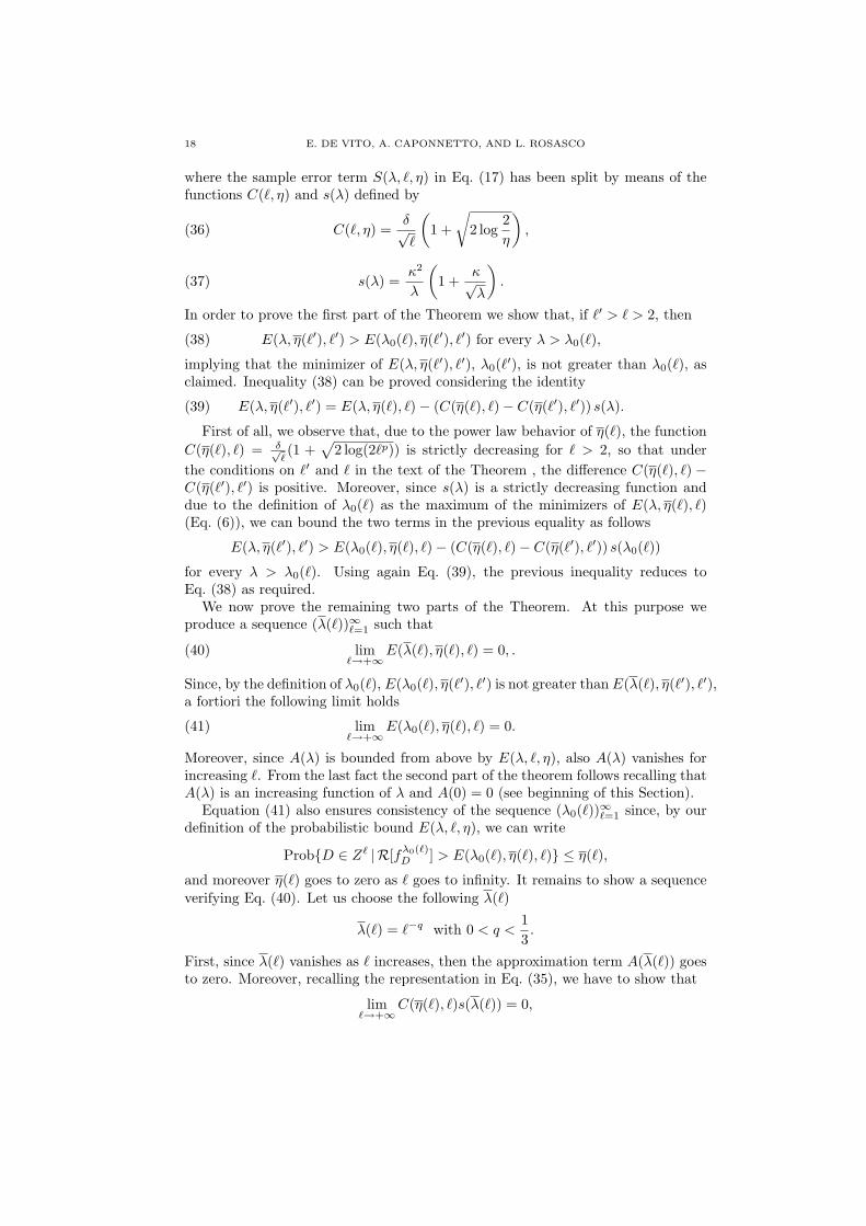
18 E. DE VITO, A. CAPONNETTO, AND L. ROSASCO

where the sample error term S(λ, `, η) in Eq. (17) has been split by means of thefunctions C(`, η) and s(λ) defined by

C(`, η) =δ√`

(1 +

√2 log

2η

),(36)

s(λ) =κ2

λ

(1 +

κ√λ

).(37)

In order to prove the first part of the Theorem we show that, if `′ > ` > 2, then

E(λ, η(`′), `′) > E(λ0(`), η(`′), `′) for every λ > λ0(`),(38)

implying that the minimizer of E(λ, η(`′), `′), λ0(`′), is not greater than λ0(`), asclaimed. Inequality (38) can be proved considering the identity

E(λ, η(`′), `′) = E(λ, η(`), `)− (C(η(`), `)− C(η(`′), `′)) s(λ).(39)

First of all, we observe that, due to the power law behavior of η(`), the functionC(η(`), `) = δ√

`(1 +

√2 log(2`p)) is strictly decreasing for ` > 2, so that under

the conditions on `′ and ` in the text of the Theorem , the difference C(η(`), `) −C(η(`′), `′) is positive. Moreover, since s(λ) is a strictly decreasing function anddue to the definition of λ0(`) as the maximum of the minimizers of E(λ, η(`), `)(Eq. (6)), we can bound the two terms in the previous equality as follows

E(λ, η(`′), `′) > E(λ0(`), η(`), `)− (C(η(`), `)− C(η(`′), `′)) s(λ0(`))

for every λ > λ0(`). Using again Eq. (39), the previous inequality reduces toEq. (38) as required.

We now prove the remaining two parts of the Theorem. At this purpose weproduce a sequence (λ(`))∞`=1 such that

lim`→+∞

E(λ(`), η(`), `) = 0, .(40)

Since, by the definition of λ0(`), E(λ0(`), η(`′), `′) is not greater than E(λ(`), η(`′), `′),a fortiori the following limit holds

lim`→+∞

E(λ0(`), η(`), `) = 0.(41)

Moreover, since A(λ) is bounded from above by E(λ, `, η), also A(λ) vanishes forincreasing `. From the last fact the second part of the theorem follows recalling thatA(λ) is an increasing function of λ and A(0) = 0 (see beginning of this Section).

Equation (41) also ensures consistency of the sequence (λ0(`))∞`=1 since, by ourdefinition of the probabilistic bound E(λ, `, η), we can write

Prob{D ∈ Z` |R[fλ0(`)D ] > E(λ0(`), η(`), `)} ≤ η(`),

and moreover η(`) goes to zero as ` goes to infinity. It remains to show a sequenceverifying Eq. (40). Let us choose the following λ(`)

λ(`) = `−q with 0 < q <13.

First, since λ(`) vanishes as ` increases, then the approximation term A(λ(`)) goesto zero. Moreover, recalling the representation in Eq. (35), we have to show that

lim`→+∞

C(η(`), `)s(λ(`)) = 0,

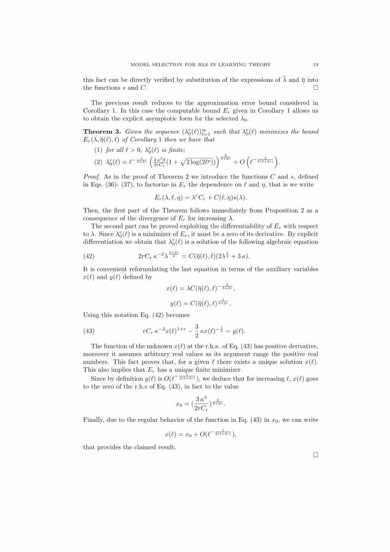
MODEL SELECTION FOR RLS IN LEARNING THEORY 19

this fact can be directly verified by substitution of the expressions of λ and η intothe functions s and C. �

The previous result reduces to the approximation error bound considered inCorollary 1. In this case the computable bound Er given in Corollary 1 allows usto obtain the explicit asymptotic form for the selected λ0.

Theorem 3. Given the sequence (λr0(`))

∞`=1 such that λr

0(`) minimizes the boundEr(λ, η(`), `) of Corollary 1 then we have that

(1) for all ` > 0, λr0(`) is finite;

(2) λr0(`) = `−

13+2r

(3 κ3δ2rCr

(1 +√

2 log(2`p))) 2

3+2r

+ O(`−

32(3+2r)

).

Proof. As in the proof of Theorem 2 we introduce the functions C and s, definedin Eqs. (36)- (37), to factorize in Er the dependence on ` and η, that is we write

Er(λ, `, η) = λrCr + C(`, η)s(λ).

Then, the first part of the Theorem follows immediately from Proposition 2 as aconsequence of the divergence of Er for increasing λ.

The second part can be proved exploiting the differentiability of Er with respectto λ. Since λr

0(`) is a minimizer of Er, it must be a zero of its derivative. By explicitdifferentiation we obtain that λr

0(`) is a solution of the following algebraic equation

2rCr κ−2λ3+2r

2 = C(η(`), `)(2λ12 + 3 κ).(42)

It is convenient reformulating the last equation in terms of the auxiliary variablesx(`) and y(`) defined by

x(`) = λC(η(`), `)−2

3+2r ,

y(`) = C(η(`), `)1

3+2r .

Using this notation Eq. (42) becomes

rCr κ−2x(`)1+r − 32

κx(`)−12 = y(`).(43)

The function of the unknown x(`) at the r.h.s. of Eq. (43) has positive derivative,moreover it assumes arbitrary real values as its argument range the positive realnumbers. This fact proves that, for a given ` there exists a unique solution x(`).This also implies that Er has a unique finite minimizer.

Since by definition y(`) is O(`−1

2(3+2r) ), we deduce that for increasing `, x(`) goesto the zero of the r.h.s of Eq. (43), in fact to the value

x0 = (3 κ3

2rCr)

23+2r .

Finally, due to the regular behavior of the function in Eq. (43) in x0, we can write

x(`) = x0 + O(`−1

2(3+2r) ),

that provides the claimed result.�

20 E. DE VITO, A. CAPONNETTO, AND L. ROSASCO

5. Conclusions

In this paper we focus on a functional analytical approach to learning theory,in the same spirit of [7]. Unlike other studies we do not examine the deviation ofthe empirical error from the expected error, but we analyze directly the expectedrisk of the solution. As a consequence the splitting of the expected error in anestimation error term and an approximation error follows naturally giving rise to abias-variance problem.

In this paper we show a possible way to solve this problem by proposing a modelselection criterion that relies on the stability properties of the regularized least-squares algorithm and does not make direct use of any complexity measures. Inparticular our estimates depend only on a boundedness assumption on the outputspace and the kernel.

Our analysis uses extensively the special properties of the square loss function,henceforth it would be interesting to extend our approach to other loss functions.We think that our results may be improved by taking into account more informationabout the structure of the hypothesis space.

Acknowledgment 1. We thank for many useful discussions and suggestions MichelePiana, Alessandro Verri and the referees. L. Rosasco is supported by an INFMfellowship. A. Caponnetto is supported by a PRIN fellowship within the project“Inverse problems in medical imaging”, n. 2002013422. This research has beenpartially funded by the INFM Project MAIA, the FIRB Project ASTA, and by theEU Project KerMIT.

Appendix A. Bounding the approximation error

In this appendix we report an elementary proof of the following result fromapproximation theory.

Theorem 4. Assume that there is r ∈ (0, 1] such that Pf0 is in the domain of L−rν

and let Cr be a constant such that ‖L−rν Pf0‖ν ≤ Cr. Then,

R[fλ] ≤ λrCr.

Proof. Starting from Eq. (21) in section 3.3 and the definition of Cr we just haveto show that ∥∥fλ − Pf0

∥∥ν≤ λr

∥∥L−rν Pf0

∥∥ν.

Due to the fact that K is a Mercer kernel, Lν is a compact positive operator and,by spectral decomposition of Lν , there is a sequence (φn)N

n=1 in L2(X, ν) (possiblyN = +∞) such that

〈φn, φm〉ν = δnm

Lνf =N∑

n=1

σ2n 〈f, φn〉ν φn,

where σn ≥ σn+1 > 0. In particular, (φn)Ni=1 is a orthonormal basis of the range of

P .Moreover, since the function g(x) = xr is a concave function on (0,+∞) and

g′(1) = r, then

(44) xr ≤ r(x− 1) + 1 ≤ x + 1.

MODEL SELECTION FOR RLS IN LEARNING THEORY 21

Recalling thatfλ = (Lν + λ)−1Lνf0,

∥∥fλ − Pf0

∥∥2

ν=

N∑n=1

⟨((Lν + λ)−1

Lν − I)

Pf0, φn

⟩2

ν

=N∑

n=1

(σ2

n

σ2n + λ

− 1)2

〈Pf0, φn〉2ν

(xn =σ2

n

λ) =

N∑n=1

(1

xn + 1

)2

〈Pf0, φn〉2ν

(Eq. (44)) ≤N∑

n=1

(1xr

n

)2

〈Pf0, φn〉2ν

= λ2rN∑

n=1

(1

(σ2n)r

)2

〈Pf0, φn〉2ν

= λ2r∥∥L−r

ν Pf0

∥∥2

ν.

�

References

[1] N. Alon, S. Ben-David, N. Cesa-Bianchi, and D. Haussler, Scale-sensitive dimensions, uniformconvergence, and learnability, J. ACM 44 (1997), 615–631.

[2] N. Aronszajn, Theory of reproducing kernels, Trans. Amer. Math. Soc. 68 (1950), 337–404.[3] P. Bartlett, S. Boucheron, and G. Lugosi, Model selection and error estimation, Machine

Learning 48 (2002), 85–113.

[4] O. Bousquet and A. Elisseeff, Stability and generalization, J. Mach. Learn. Res. 2 (2002),499–526.

[5] N. Cristianini and J. Shawe Taylor, An Introduction to Support Vector Machines, CambridgeUniversity Press, Cambridge, UK, 2000.

[6] F. Cucker and S. Smale, Best choices for regularization parameters in learning theory: on the

bias-variance problem, Found. Comput. Math. 2 (2002), 413–428.[7] F. Cucker and S. Smale, On the mathematical foundations of learning, Bull. Amer. Math.

Soc. (N.S.) 39 (2002), 1–49 (electronic).

[8] L. Devroye, L. Gyorfi, and G. Lugosi, A probabilistic theory of pattern recognition, Springer-Verlag, New York, 1996.

[9] R. Dudley, Real analysis and probability, Cambridge University Press, Cambridge, 2002.

[10] T. Evgeniou, M. Pontil, and T. Poggio, Regularization networks and support vector machines,Adv. Comput. Math. 13 (2000), 1–50.

[11] F. Girosi, M. Jones, and T. Poggio, Regularization theory and neural networks architectures,

Neural Computation 7 (1995), 219–269.[12] T. Hastie, R. Tibshirani, and J. Friedman, The elements of statistical learning, Springer-

Verlag, New York, 2001.[13] C. McDiarmid, On the method of bounded differences, In Surveys in combinatorics, 1989

(Norwich, 1989), Cambridge Univ. Press, Cambridge, 1989, pp. 148–188.

[14] S. Mendelson, A few notes on statistical learning theory, In S. Mendelson and A. Smola,editors, Advanced Lectures in Machine Learning, Springer-Verlag, 2003, pp. 1–40.

[15] P. Niyogi and F. Girosi, Generalization bounds for function approximation from scattered

noisy data, Adv. Comput. Math. 10 (1999), 51–80.[16] T. Poggio and F. Girosi, Networks for approximation and learning, In Proceedings of the

IEEE, volume 78, 1990, pp. 1481–1497.

[17] T. Poggio, R. Rifkin, S. Mukherjee, and P. Niyogi, General conditions for predictivity inlearning theory, Nature 428 (2004), 419–422.

22 E. DE VITO, A. CAPONNETTO, AND L. ROSASCO

[18] L. Rosasco, E. De Vito, A. Caponnetto, M. Piana, and A. Verri, Are loss functions all thesame?, Neural Computation 16 (2004), 1063–1076.

[19] S. Smale and D.-X. Zhou, Estimating the approximation error in learning theory, Anal. Appl.

(Singap.) 1 (2003), 17–41.[20] I. Steinwart, Consistency of support vector machines and other regularized kernel machines,

Technical Report 02-03, University of Jena, Department of Mathematics and Computer Sci-ence, 2002.

[21] V. Vapnik, Statistical learning theory, John Wiley & Sons Inc., New York, 1998.

[22] G. Wahba, Spline models for observational data, Society for Industrial and Applied Mathe-matics (SIAM), Philadelphia, PA, 1990.

[23] T. Zhang, Leave-one-out bounds for kenrel methods, Neural Computation 15 (2003), 1397–

1437.[24] D.-X. Zhou, The covering number in learning theory, J. Complexity 18 (2002), 739–767.

Ernesto De Vito, Dipartimento di Matematica, Universita di Modena, Via Campi213/B, 41100 Modena, Italy and I.N.F.N., Sezione di Genova, Via Dodecaneso 33, 16146Genova, Italy,

E-mail address: devito@unimo.it

Andrea Caponnetto, D.I.S.I., Universita di Genova, Via Dodecaneso 35, 16146 Gen-ova, Italy, and I.N.F.M., Sezione di Genova, Via Dodecaneso 33, 16146 Genova, Italy

E-mail address: caponnetto@disi.unige.it

Lorenzo Rosasco, D.I.S.I., Universita di Genova, Via Dodecaneso 35, 16146 Genova,

Italy, and I.N.F.M., Sezione di Genova, Via Dodecaneso 33, 16146 Genova, ItalyE-mail address: rosasco@disi.unige.it