Model for fitting longitudinal traits subject to threshold response applied to genetic evaluation...
9
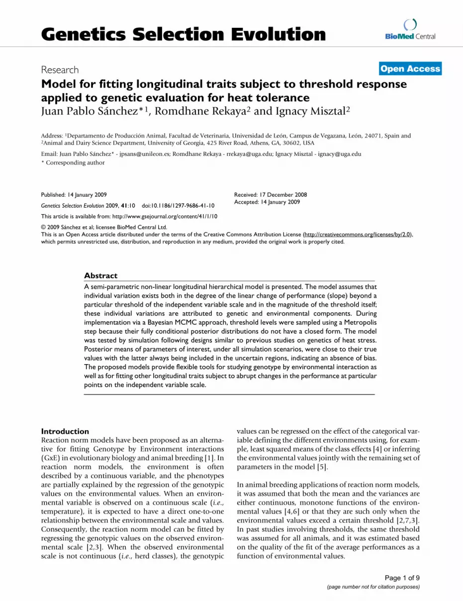
BioMed Central Page 1 of 9 (page number not for citation purposes) Genetics Selection Evolution Open Access Research Model for fitting longitudinal traits subject to threshold response applied to genetic evaluation for heat tolerance Juan Pablo Sánchez* 1 , Romdhane Rekaya 2 and Ignacy Misztal 2 Address: 1 Departamento de Producción Animal, Facultad de Veterinaria, Universidad de León, Campus de Vegazana, León, 24071, Spain and 2 Animal and Dairy Science Department, University of Georgia, 425 River Road, Athens, GA, 30602, USA Email: Juan Pablo Sánchez* - [email protected]; Romdhane Rekaya - [email protected]; Ignacy Misztal - [email protected] * Corresponding author Abstract A semi-parametric non-linear longitudinal hierarchical model is presented. The model assumes that individual variation exists both in the degree of the linear change of performance (slope) beyond a particular threshold of the independent variable scale and in the magnitude of the threshold itself; these individual variations are attributed to genetic and environmental components. During implementation via a Bayesian MCMC approach, threshold levels were sampled using a Metropolis step because their fully conditional posterior distributions do not have a closed form. The model was tested by simulation following designs similar to previous studies on genetics of heat stress. Posterior means of parameters of interest, under all simulation scenarios, were close to their true values with the latter always being included in the uncertain regions, indicating an absence of bias. The proposed models provide flexible tools for studying genotype by environmental interaction as well as for fitting other longitudinal traits subject to abrupt changes in the performance at particular points on the independent variable scale. Introduction Reaction norm models have been proposed as an alterna- tive for fitting Genotype by Environment interactions (GxE) in evolutionary biology and animal breeding [1]. In reaction norm models, the environment is often described by a continuous variable, and the phenotypes are partially explained by the regression of the genotypic values on the environmental values. When an environ- mental variable is observed on a continuous scale (i.e., temperature), it is expected to have a direct one-to-one relationship between the environmental scale and values. Consequently, the reaction norm model can be fitted by regressing the genotypic values on the observed environ- mental scale [2,3]. When the observed environmental scale is not continuous (i.e., herd classes), the genotypic values can be regressed on the effect of the categorical var- iable defining the different environments using, for exam- ple, least squared means of the class effects [4] or inferring the environmental values jointly with the remaining set of parameters in the model [5]. In animal breeding applications of reaction norm models, it was assumed that both the mean and the variances are either continuous, monotone functions of the environ- mental values [4,6] or that they are such only when the environmental values exceed a certain threshold [2,7,3]. In past studies involving thresholds, the same threshold was assumed for all animals, and it was estimated based on the quality of the fit of the average performances as a function of environmental values. Published: 14 January 2009 Genetics Selection Evolution 2009, 41:10 doi:10.1186/1297-9686-41-10 Received: 17 December 2008 Accepted: 14 January 2009 This article is available from: http://www.gsejournal.org/content/41/1/10 © 2009 Sánchez et al; licensee BioMed Central Ltd. This is an Open Access article distributed under the terms of the Creative Commons Attribution License (http://creativecommons.org/licenses/by/2.0 ), which permits unrestricted use, distribution, and reproduction in any medium, provided the original work is properly cited.
-
Upload
juan-pablo-sanchez -
Category
Documents
-
view
213 -
download
1
Transcript of Model for fitting longitudinal traits subject to threshold response applied to genetic evaluation...
BioMed CentralGenetics Selection Evolution
ss
Open AcceResearchModel for fitting longitudinal traits subject to threshold response applied to genetic evaluation for heat toleranceJuan Pablo Sánchez*1, Romdhane Rekaya2 and Ignacy Misztal2Address: 1Departamento de Producción Animal, Facultad de Veterinaria, Universidad de León, Campus de Vegazana, León, 24071, Spain and 2Animal and Dairy Science Department, University of Georgia, 425 River Road, Athens, GA, 30602, USA
Email: Juan Pablo Sánchez* - [email protected]; Romdhane Rekaya - [email protected]; Ignacy Misztal - [email protected]
* Corresponding author
AbstractA semi-parametric non-linear longitudinal hierarchical model is presented. The model assumes thatindividual variation exists both in the degree of the linear change of performance (slope) beyond aparticular threshold of the independent variable scale and in the magnitude of the threshold itself;these individual variations are attributed to genetic and environmental components. Duringimplementation via a Bayesian MCMC approach, threshold levels were sampled using a Metropolisstep because their fully conditional posterior distributions do not have a closed form. The modelwas tested by simulation following designs similar to previous studies on genetics of heat stress.Posterior means of parameters of interest, under all simulation scenarios, were close to their truevalues with the latter always being included in the uncertain regions, indicating an absence of bias.The proposed models provide flexible tools for studying genotype by environmental interaction aswell as for fitting other longitudinal traits subject to abrupt changes in the performance at particularpoints on the independent variable scale.
IntroductionReaction norm models have been proposed as an alterna-tive for fitting Genotype by Environment interactions(GxE) in evolutionary biology and animal breeding [1]. Inreaction norm models, the environment is oftendescribed by a continuous variable, and the phenotypesare partially explained by the regression of the genotypicvalues on the environmental values. When an environ-mental variable is observed on a continuous scale (i.e.,temperature), it is expected to have a direct one-to-onerelationship between the environmental scale and values.Consequently, the reaction norm model can be fitted byregressing the genotypic values on the observed environ-mental scale [2,3]. When the observed environmentalscale is not continuous (i.e., herd classes), the genotypic
values can be regressed on the effect of the categorical var-iable defining the different environments using, for exam-ple, least squared means of the class effects [4] or inferringthe environmental values jointly with the remaining set ofparameters in the model [5].
In animal breeding applications of reaction norm models,it was assumed that both the mean and the variances areeither continuous, monotone functions of the environ-mental values [4,6] or that they are such only when theenvironmental values exceed a certain threshold [2,7,3].In past studies involving thresholds, the same thresholdwas assumed for all animals, and it was estimated basedon the quality of the fit of the average performances as afunction of environmental values.
Published: 14 January 2009
Genetics Selection Evolution 2009, 41:10 doi:10.1186/1297-9686-41-10
Received: 17 December 2008Accepted: 14 January 2009
This article is available from: http://www.gsejournal.org/content/41/1/10
© 2009 Sánchez et al; licensee BioMed Central Ltd. This is an Open Access article distributed under the terms of the Creative Commons Attribution License (http://creativecommons.org/licenses/by/2.0), which permits unrestricted use, distribution, and reproduction in any medium, provided the original work is properly cited.
Page 1 of 9(page number not for citation purposes)
Genetics Selection Evolution 2009, 41:10 http://www.gsejournal.org/content/41/1/10
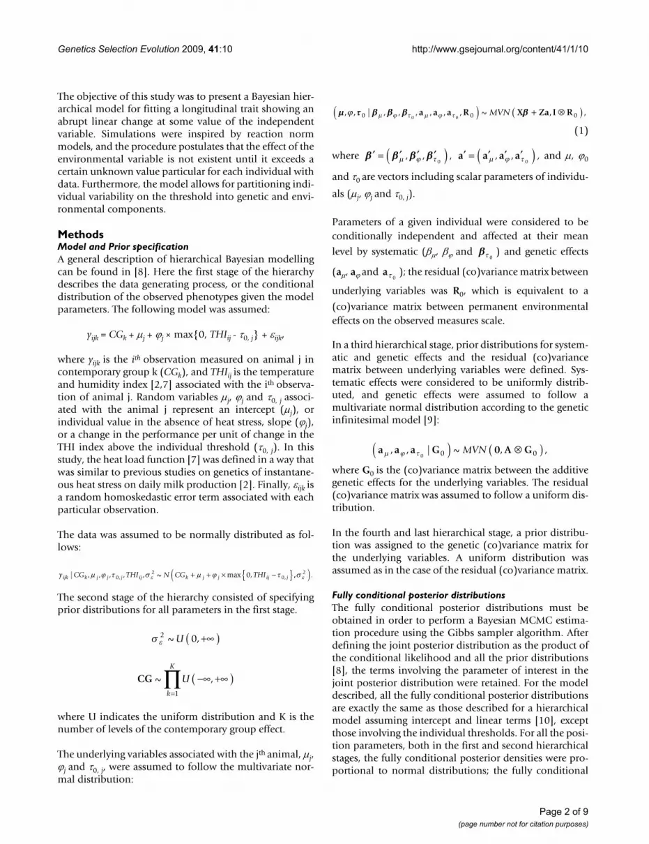
The objective of this study was to present a Bayesian hier-archical model for fitting a longitudinal trait showing anabrupt linear change at some value of the independentvariable. Simulations were inspired by reaction normmodels, and the procedure postulates that the effect of theenvironmental variable is not existent until it exceeds acertain unknown value particular for each individual withdata. Furthermore, the model allows for partitioning indi-vidual variability on the threshold into genetic and envi-ronmental components.
MethodsModel and Prior specificationA general description of hierarchical Bayesian modellingcan be found in [8]. Here the first stage of the hierarchydescribes the data generating process, or the conditionaldistribution of the observed phenotypes given the modelparameters. The following model was assumed:
yijk = CGk + j + j × max{0, THIij - 0, j} + ijk,
where yijk is the ith observation measured on animal j incontemporary group k (CGk), and THIij is the temperatureand humidity index [2,7] associated with the ith observa-tion of animal j. Random variables j, j and 0, j associ-ated with the animal j represent an intercept (j), orindividual value in the absence of heat stress, slope (j),or a change in the performance per unit of change in theTHI index above the individual threshold (0, j). In thisstudy, the heat load function [7] was defined in a way thatwas similar to previous studies on genetics of instantane-ous heat stress on daily milk production [2]. Finally, ijk isa random homoskedastic error term associated with eachparticular observation.
The data was assumed to be normally distributed as fol-lows:
The second stage of the hierarchy consisted of specifyingprior distributions for all parameters in the first stage.
where U indicates the uniform distribution and K is thenumber of levels of the contemporary group effect.
The underlying variables associated with the jth animal, j,j and 0, j, were assumed to follow the multivariate nor-mal distribution:
where , , and , 0
and 0 are vectors including scalar parameters of individu-
als (j, j and 0, j).
Parameters of a given individual were considered to beconditionally independent and affected at their mean
level by systematic (, and ) and genetic effects
(a, a and ); the residual (co)variance matrix between
underlying variables was R0, which is equivalent to a
(co)variance matrix between permanent environmentaleffects on the observed measures scale.
In a third hierarchical stage, prior distributions for system-atic and genetic effects and the residual (co)variancematrix between underlying variables were defined. Sys-tematic effects were considered to be uniformly distrib-uted, and genetic effects were assumed to follow amultivariate normal distribution according to the geneticinfinitesimal model [9]:
where G0 is the (co)variance matrix between the additivegenetic effects for the underlying variables. The residual(co)variance matrix was assumed to follow a uniform dis-tribution.
In the fourth and last hierarchical stage, a prior distribu-tion was assigned to the genetic (co)variance matrix forthe underlying variables. A uniform distribution wasassumed as in the case of the residual (co)variance matrix.
Fully conditional posterior distributionsThe fully conditional posterior distributions must beobtained in order to perform a Bayesian MCMC estima-tion procedure using the Gibbs sampler algorithm. Afterdefining the joint posterior distribution as the product ofthe conditional likelihood and all the prior distributions[8], the terms involving the parameter of interest in thejoint posterior distribution were retained. For the modeldescribed, all the fully conditional posterior distributionsare exactly the same as those described for a hierarchicalmodel assuming intercept and linear terms [10], exceptthose involving the individual thresholds. For all the posi-tion parameters, both in the first and second hierarchicalstages, the fully conditional posterior densities were pro-portional to normal distributions; the fully conditional
y CG THI N CG THIijk k j j j ij k j j ij j| , , , , , ~ max ,, , 02
00+ + × −{ } ,, . 2( )
2 0~ ,U +∞( )
CG ~ ,Uk
K
−∞ +∞( )=
∏1
, , | , , , , , , ~ , , 0 0 00 0a a a R X Za I R( ) + ⊗( )MVN
(1)
′ = ′ ′ ′( ) , ,0
′ = ′ ′ ′( )a a a a , ,0
0
a 0
a a a G 0 A G , , | ~ , ,0 0 0( ) ⊗( )MVN
Page 2 of 9(page number not for citation purposes)
Genetics Selection Evolution 2009, 41:10 http://www.gsejournal.org/content/41/1/10
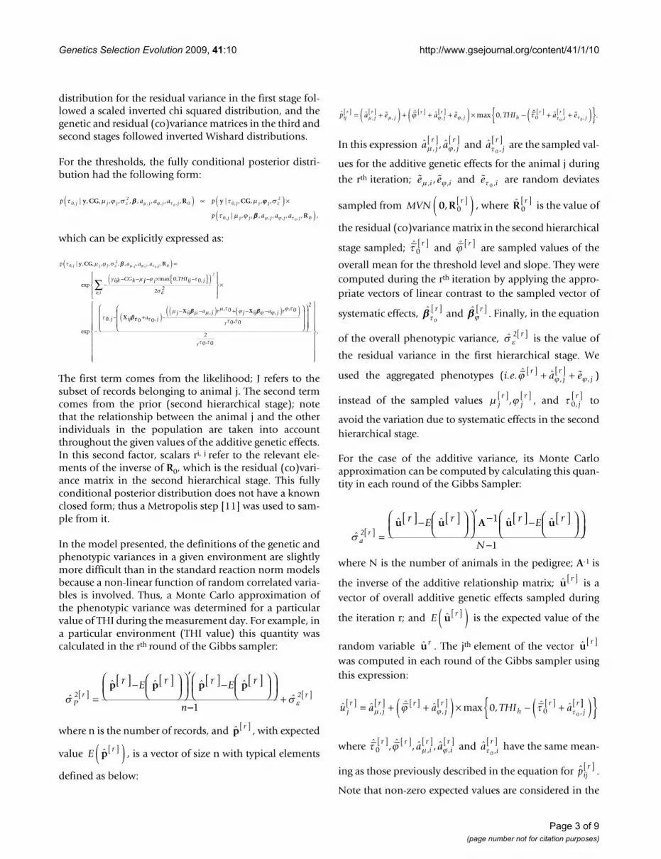
distribution for the residual variance in the first stage fol-lowed a scaled inverted chi squared distribution, and thegenetic and residual (co)variance matrices in the third andsecond stages followed inverted Wishard distributions.
For the thresholds, the fully conditional posterior distri-bution had the following form:
which can be explicitly expressed as:
The first term comes from the likelihood; J refers to thesubset of records belonging to animal j. The second termcomes from the prior (second hierarchical stage); notethat the relationship between the animal j and the otherindividuals in the population are taken into accountthroughout the given values of the additive genetic effects.In this second factor, scalars ri, j refer to the relevant ele-ments of the inverse of R0, which is the residual (co)vari-ance matrix in the second hierarchical stage. This fullyconditional posterior distribution does not have a knownclosed form; thus a Metropolis step [11] was used to sam-ple from it.
In the model presented, the definitions of the genetic andphenotypic variances in a given environment are slightlymore difficult than in the standard reaction norm modelsbecause a non-linear function of random correlated varia-bles is involved. Thus, a Monte Carlo approximation ofthe phenotypic variance was determined for a particularvalue of THI during the measurement day. For example, ina particular environment (THI value) this quantity wascalculated in the rth round of the Gibbs sampler:
where n is the number of records, and , with expected
value , is a vector of size n with typical elements
defined as below:
In this expression and are the sampled val-
ues for the additive genetic effects for the animal j during
the rth iteration; and are random deviates
sampled from , where is the value of
the residual (co)variance matrix in the second hierarchical
stage sampled; and are sampled values of the
overall mean for the threshold level and slope. They werecomputed during the rth iteration by applying the appro-priate vectors of linear contrast to the sampled vector of
systematic effects, and . Finally, in the equation
of the overall phenotypic variance, is the value of
the residual variance in the first hierarchical stage. We
used the aggregated phenotypes (i.e. )
instead of the sampled values , and to
avoid the variation due to systematic effects in the secondhierarchical stage.
For the case of the additive variance, its Monte Carloapproximation can be computed by calculating this quan-tity in each round of the Gibbs Sampler:
where N is the number of animals in the pedigree; A-1 is
the inverse of the additive relationship matrix; is avector of overall additive genetic effects sampled during
the iteration r; and is the expected value of the
random variable . The jth element of the vector was computed in each round of the Gibbs sampler usingthis expression:
where and have the same mean-
ing as those previously described in the equation for .
Note that non-zero expected values are considered in the
p a a a pj j j j j j j j 02
0 00, , , , ,| , , , , , , , , , | , , ,y CG R y CG( ) ∝
j
j j j j j jp a a a
,
| , , , , , , ,, , , ,
2
0 00
( ) ×
( ) R
p a a a
yijk CGk
j j j j j j
02
00, , , ,| , , , , , , , , ,
exp
y CG R( ) ∝
−− − jj j THIij j
j ij
i J
− × −{ }( )⎧
⎨⎪
⎩⎪
⎫
⎬⎪
⎭⎪
×
−
−
∈∑
max , ,
exp
,
0 0
2 2
0
2
X
0 0
0 0
0+( )−
− −( ) + − −( )( )a j
j ij a j r j ij a j r
r,
,,
,,X X
,,
,
0
2
2
0 0
⎛
⎝
⎜⎜⎜
⎞
⎠
⎟⎟⎟
⎛
⎝
⎜⎜⎜⎜
⎞
⎠
⎟⎟⎟⎟
⎧
⎨
⎪⎪⎪⎪⎪
⎩
⎪⎪⎪⎪⎪
⎫
⎬
⎪⎪⎪⎪⎪
⎭
⎪⎪⎪
r
⎪⎪⎪
,
ˆˆ ˆ ˆ ˆ
Pr
r E r r E r
n2[ ] =
[ ]− [ ]⎛⎝⎜
⎞⎠⎟
⎛⎝⎜
⎞⎠⎟′ [ ]− [ ]⎛
⎝⎜⎞⎠⎟
⎛⎝⎜
⎞⎠⎟
p p p p
−−+ [ ]
12
r
p r[ ]
E rp[ ]( )
ˆ ˆ ˆ ˆ max ,, , , ,p a e a e THIijr
jr
jr
jr
j h[ ] [ ] [ ] [ ]= +( ) + + +( ) × − 0 ˆ ˆ ., , 0 0 0
ri
rja e[ ] [ ]+ +( ){ }
ˆ , ˆ, ,a ajr
jr
[ ] [ ] ˆ
,a jr
0
[ ]
e ei i , ,, e i 0 ,
MVN r0 R, 0[ ]( ) R 0
r[ ]
0r[ ] r[ ]
0
r[ ] r[ ]
2 r[ ]
ˆ ˆ , , r
jr
ja e[ ] [ ]+ +
jr
jr[ ] [ ], 0, j
r[ ]
ˆˆ ˆ ˆ ˆ
ar
r E r r E r2
1[ ] =
[ ]− [ ]⎛⎝⎜
⎞⎠⎟
⎛⎝⎜
⎞⎠⎟′ − [ ]− [ ]⎛
⎝⎜⎞⎠⎟
⎛⎝⎜
⎞u u A u u
⎠⎠⎟
−N 1
u r[ ]
E ru[ ]( )u r u r[ ]
ˆ ˆ ˆ ˆ max , ˆ ˆ, , ,u a a THI ajr
jr r
jr
hr
jr[ ] [ ] [ ] [ ] [ ] [= + +( ) × − + 0 0 0
]]( ){ }ˆ , ˆ , ˆ , ˆ, , 0
r ri
ri
ra a[ ] [ ] [ ] [ ] ˆ,a i
r 0
[ ]
pijr[ ]
Page 3 of 9(page number not for citation purposes)
Genetics Selection Evolution 2009, 41:10 http://www.gsejournal.org/content/41/1/10
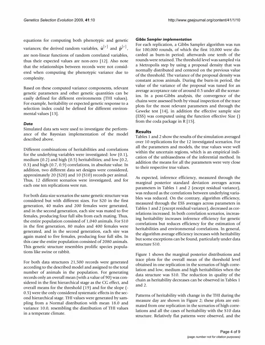
equations for computing both phenotypic and genetic
variances; the derived random variables, and ,
are non-linear functions of random correlated variables,thus their expected values are non-zero [12]. Also notethat the relationships between records were not consid-ered when computing the phenotypic variance due tocomplexity.
Based on these computed variance components, relevantgenetic parameters and other genetic quantities can beeasily defined for different environments (THI values).For example, heritability or expected genetic response to aselection index could be defined for different environ-mental values [13].
DataSimulated data sets were used to investigate the perform-ance of the Bayesian implementation of the modeldescribed above.
Different combinations of heritabilities and correlationsfor the underlying variables were investigated: low (0.1),medium (0.2) and high (0.5) heritabilities; and low (0.2,0.3) and high (0.7, 0.9) correlations, in absolute value. Inaddition, two different data set designs were considered,approximately 20 (S20) and 10 (S10) records per animal.Thus, 12 different scenarios were investigated, and foreach one ten replications were run.
For both data size scenarios the same genetic structure wasconsidered but with different sizes. For S20 in the firstgeneration, 40 males and 200 females were generated,and in the second generation, each sire was mated to fivefemales, producing four full sibs from each mating. Thus,the entire population consisted of 1,040 animals. For S10in the first generation, 80 males and 400 females weregenerated, and in the second generation, each sire wasagain mated to five females, producing four full sibs. Inthis case the entire population consisted of 2080 animals.This genetic structure resembles prolific species popula-tions like swine or rabbit.
For both data structures 21,500 records were generatedaccording to the described model and assigned to the totalnumber of animals in the population. For generatingrecords only an overall mean (with a value of 90) was con-sidered in the first hierarchical stage as the CG effect, andoverall means for the threshold (19) and for the slope (-0.5) were the only considered systematic effects in the sec-ond hierarchical stage. THI values were generated by sam-pling from a Normal distribution with mean 18.0 andvariance 10.0, resembling the distribution of THI valuesin a temperate climate.
Gibbs Sampler implementationFor each replication, a Gibbs Sampler algorithm was runfor 100,000 rounds, of which the first 10,000 were dis-carded as burn-in period; afterwards one tenth of therounds were retained. The threshold level was sampled viaa Metropolis step by using a proposal density that wasnormally distributed and centered on the previous valueof the threshold. The variance of the proposal density wasconstant across animals. During the burn-in period, thevalue of the variance of the proposal was tuned for anaverage acceptance rate of around 0.5 under all the scenar-ios. In a post-Gibbs analysis, the convergence of thechains were assessed both by visual inspection of the traceplots for the most relevant parameters and through theGeweke test [14], in addition the effective sample size(ESS) was computed using the function effective Size ()from the coda package in R [15].
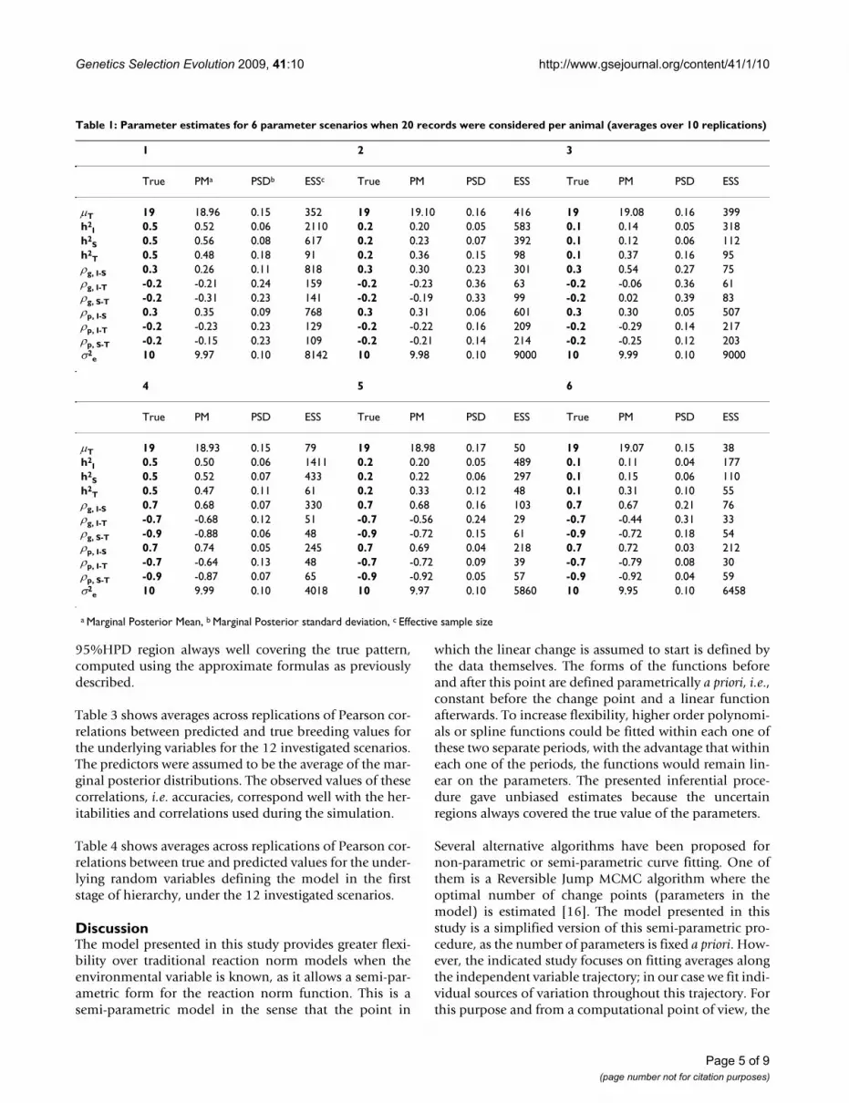
ResultsTables 1 and 2 show the results of the simulation averagedover 10 replications for the 12 investigated scenarios. Forall the parameters and models, the true values were wellwithin the uncertain regions, which is an empirical indi-cation of the unbiasedness of the inferential method. Inaddition the means for all the parameters were very closeto their respective true values.
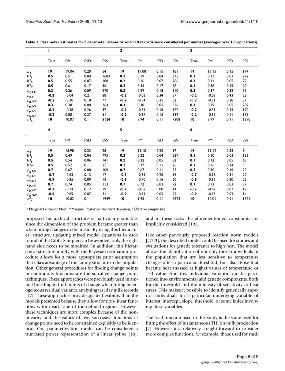
As expected, inference efficiency, measured through themarginal posterior standard deviation averages acrossparameters in Tables 1 and 2 (except residual variance),was reduced as the correlations between underlying varia-bles was reduced. On the contrary, algorithm efficiency,measured through the ESS averages across parameters inTables 1 and 2 (except residual variance), decreased as cor-relations increased. In both correlation scenarios, increas-ing heritability increases inference efficiency for geneticcorrelations but reduces efficiency for the estimation ofheritabilities and environmental correlations. In general,the algorithm average efficiency increases with heritabilitybut some exceptions can be found, particularly under datastructure S10.
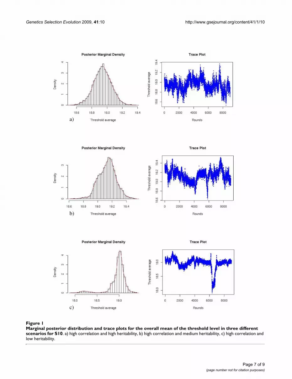
Figure 1 shows the marginal posterior distributions andtrace plots for the overall mean of the threshold levelobtained in one replication in the scenarios of high corre-lation and low, medium and high heritabilities when thedata structure was S10. The reduction in quality of thechain as heritability decreases can be observed in Tables 1and 2.
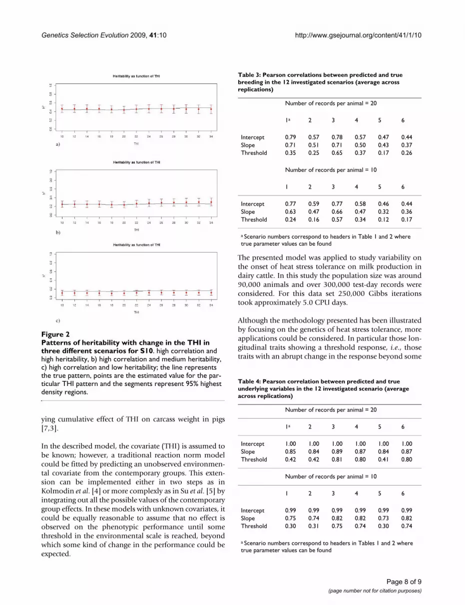
Patterns of heritability with change in the THI during themeasure day are shown in Figure 2; these plots are esti-mated from one replication in the scenarios of high corre-lations and all the cases of heritability with the S10 datastructure. Relatively flat patterns were observed, and the
u r[ ] p r[ ]
Page 4 of 9(page number not for citation purposes)
Genetics Selection Evolution 2009, 41:10 http://www.gsejournal.org/content/41/1/10
95%HPD region always well covering the true pattern,computed using the approximate formulas as previouslydescribed.
Table 3 shows averages across replications of Pearson cor-relations between predicted and true breeding values forthe underlying variables for the 12 investigated scenarios.The predictors were assumed to be the average of the mar-ginal posterior distributions. The observed values of thesecorrelations, i.e. accuracies, correspond well with the her-itabilities and correlations used during the simulation.
Table 4 shows averages across replications of Pearson cor-relations between true and predicted values for the under-lying random variables defining the model in the firststage of hierarchy, under the 12 investigated scenarios.
DiscussionThe model presented in this study provides greater flexi-bility over traditional reaction norm models when theenvironmental variable is known, as it allows a semi-par-ametric form for the reaction norm function. This is asemi-parametric model in the sense that the point in
which the linear change is assumed to start is defined bythe data themselves. The forms of the functions beforeand after this point are defined parametrically a priori, i.e.,constant before the change point and a linear functionafterwards. To increase flexibility, higher order polynomi-als or spline functions could be fitted within each one ofthese two separate periods, with the advantage that withineach one of the periods, the functions would remain lin-ear on the parameters. The presented inferential proce-dure gave unbiased estimates because the uncertainregions always covered the true value of the parameters.
Several alternative algorithms have been proposed fornon-parametric or semi-parametric curve fitting. One ofthem is a Reversible Jump MCMC algorithm where theoptimal number of change points (parameters in themodel) is estimated [16]. The model presented in thisstudy is a simplified version of this semi-parametric pro-cedure, as the number of parameters is fixed a priori. How-ever, the indicated study focuses on fitting averages alongthe independent variable trajectory; in our case we fit indi-vidual sources of variation throughout this trajectory. Forthis purpose and from a computational point of view, the
Table 1: Parameter estimates for 6 parameter scenarios when 20 records were considered per animal (averages over 10 replications)
1 2 3
True PMa PSDb ESSc True PM PSD ESS True PM PSD ESS
T 19 18.96 0.15 352 19 19.10 0.16 416 19 19.08 0.16 399h2
I 0.5 0.52 0.06 2110 0.2 0.20 0.05 583 0.1 0.14 0.05 318h2
S 0.5 0.56 0.08 617 0.2 0.23 0.07 392 0.1 0.12 0.06 112h2
T 0.5 0.48 0.18 91 0.2 0.36 0.15 98 0.1 0.37 0.16 95g, I-S 0.3 0.26 0.11 818 0.3 0.30 0.23 301 0.3 0.54 0.27 75g, I-T -0.2 -0.21 0.24 159 -0.2 -0.23 0.36 63 -0.2 -0.06 0.36 61g, S-T -0.2 -0.31 0.23 141 -0.2 -0.19 0.33 99 -0.2 0.02 0.39 83p, I-S 0.3 0.35 0.09 768 0.3 0.31 0.06 601 0.3 0.30 0.05 507p, I-T -0.2 -0.23 0.23 129 -0.2 -0.22 0.16 209 -0.2 -0.29 0.14 217p, S-T -0.2 -0.15 0.23 109 -0.2 -0.21 0.14 214 -0.2 -0.25 0.12 2032
e 10 9.97 0.10 8142 10 9.98 0.10 9000 10 9.99 0.10 9000
4 5 6
True PM PSD ESS True PM PSD ESS True PM PSD ESS
T 19 18.93 0.15 79 19 18.98 0.17 50 19 19.07 0.15 38h2
I 0.5 0.50 0.06 1411 0.2 0.20 0.05 489 0.1 0.11 0.04 177h2
S 0.5 0.52 0.07 433 0.2 0.22 0.06 297 0.1 0.15 0.06 110h2
T 0.5 0.47 0.11 61 0.2 0.33 0.12 48 0.1 0.31 0.10 55g, I-S 0.7 0.68 0.07 330 0.7 0.68 0.16 103 0.7 0.67 0.21 76g, I-T -0.7 -0.68 0.12 51 -0.7 -0.56 0.24 29 -0.7 -0.44 0.31 33g, S-T -0.9 -0.88 0.06 48 -0.9 -0.72 0.15 61 -0.9 -0.72 0.18 54p, I-S 0.7 0.74 0.05 245 0.7 0.69 0.04 218 0.7 0.72 0.03 212p, I-T -0.7 -0.64 0.13 48 -0.7 -0.72 0.09 39 -0.7 -0.79 0.08 30p, S-T -0.9 -0.87 0.07 65 -0.9 -0.92 0.05 57 -0.9 -0.92 0.04 592
e 10 9.99 0.10 4018 10 9.97 0.10 5860 10 9.95 0.10 6458
a Marginal Posterior Mean, b Marginal Posterior standard deviation, c Effective sample size
Page 5 of 9(page number not for citation purposes)
Genetics Selection Evolution 2009, 41:10 http://www.gsejournal.org/content/41/1/10
proposed hierarchical structure is particularly suitable,since the dimension of the problem became greater thanwhen fitting changes in the mean. By using this hierarchi-cal structure, updating mixed model equations in eachround of the Gibbs Sampler can be avoided; only the righthand side needs to be modified. In addition, this hierar-chical structure jointly with the Bayesian estimation pro-cedure allows for a more appropriate prior assumptionthat takes advantage of the family structure in the popula-tion. Other general procedures for finding change pointsin continuous functions are the so-called change pointtechniques. These approaches were previously used in ani-mal breeding to find points of change when fitting heter-ogeneous residual variance analysing test day milk records[17]. These approaches provide greater flexibility than themodels presented because they allow for non-linear func-tions within each one of the defined regions. Howeverthese techniques are more complex because of the non-linearity and the values of two successive functions atchange points need to be constrained explicitly to be iden-tical. Our parametrization model can be considered atruncated power representation of a linear spline [18],
and in these cases the aforementioned constraints areimplicitly considered [19].
Like other previously proposed reaction norm models[2,7,3], the described model could be used for studies andevaluations for genetic tolerance to high heat. The modelallows the identification of not only those individuals inthe population that are less sensitive to temperaturechanges after a particular threshold, but also those thatbecame heat stressed at higher values of temperature orTHI value. And this individual variation can be parti-tioned into environmental and genetic components, bothfor the threshold and the intensity of sensitivity to heatstress. This makes it possible to identify genetically supe-rior individuals for a particular underlying variable ofinterest: intercept, slope, threshold, or some index involv-ing these variables.
The load function used in this study is the same used forfitting the effect of instantaneous THI on milk production[2]. However it is relatively straight forward to considermore complex functions, for example, those used for stud-
Table 2: Parameter estimates for 6 parameter scenarios when 10 records were considered per animal (averages over 10 replications)
1 2 3
True PMa PSDb ESSc True PM PSD ESS True PM PSD ESS
T 19 19.04 0.20 54 19 19.08 0.15 181 19 19.15 0.15 174h2
I 0.5 0.51 0.04 1683 0.2 0.19 0.04 675 0.1 0.11 0.03 272h2
S 0.5 0.55 0.07 188 0.2 0.26 0.07 286 0.1 0.11 0.05 79h2
T 0.5 0.61 0.17 36 0.2 0.43 0.17 58 0.1 0.38 0.15 60g, I-S 0.3 0.26 0.09 270 0.3 0.29 0.18 310 0.3 0.37 0.32 51g, I-T -0.2 -0.04 0.21 68 -0.2 -0.03 0.34 57 -0.2 -0.03 0.43 28g, S-T -0.2 -0.30 0.18 77 -0.2 -0.34 0.25 82 -0.2 -0.51 0.28 57p, I-S 0.3 0.38 0.08 264 0.3 0.30 0.05 526 0.3 0.29 0.05 289p, I-T -0.2 -0.38 0.26 37 -0.2 -0.31 0.18 122 -0.2 -0.31 0.15 120p, S-T -0.2 0.00 0.27 51 -0.2 -0.17 0.15 139 -0.2 -0.15 0.11 1752
e 10 10.07 0.11 3124 10 9.94 0.11 7308 10 9.99 0.11 6390
4 5 6
True PM PSD ESS True PM PSD ESS True PM PSD ESS
T 19 18.98 0.22 28 19 19.10 0.25 17 19 19.12 0.53 8h2
I 0.5 0.49 0.04 795 0.2 0.22 0.04 337 0.1 0.10 0.03 136h2
S 0.5 0.54 0.06 141 0.2 0.22 0.05 82 0.1 0.12 0.05 63h2
T 0.5 0.52 0.11 25 0.2 0.37 0.11 26 0.1 0.36 0.14 9g, I-S 0.7 0.67 0.08 109 0.7 0.67 0.11 55 0.7 0.70 0.19 23g, I-T -0.7 -0.63 0.13 17 -0.7 -0.39 0.25 16 -0.7 -0.18 0.31 20g, S-T -0.9 -0.85 0.09 12 -0.9 -0.70 0.16 20 -0.9 -0.65 0.20 25p, I-S 0.7 0.74 0.05 113 0.7 0.72 0.03 72 0.7 0.72 0.03 57p, I-T -0.7 -0.74 0.12 19 -0.7 -0.82 0.08 14 -0.7 -0.82 0.07 12p, S-T -0.9 -0.89 0.07 31 -0.9 -0.91 0.05 25 -0.9 -0.95 0.03 142
e 10 10.02 0.11 1949 10 9.95 0.11 2623 10 10.01 0.11 1624
a Marginal Posterior Mean, b Marginal Posterior standard deviation, c Effective sample size
Page 6 of 9(page number not for citation purposes)
Genetics Selection Evolution 2009, 41:10 http://www.gsejournal.org/content/41/1/10
Page 7 of 9(page number not for citation purposes)
Marginal posterior distribution and trace plots for the overall mean of the threshold level in three different scenarios for S10Figure 1Marginal posterior distribution and trace plots for the overall mean of the threshold level in three different scenarios for S10. a) high correlation and high heritability, b) high correlation and medium heritability, c) high correlation and low heritability.
a)
b)
c)
Genetics Selection Evolution 2009, 41:10 http://www.gsejournal.org/content/41/1/10
ying cumulative effect of THI on carcass weight in pigs[7,3].
In the described model, the covariate (THI) is assumed tobe known; however, a traditional reaction norm modelcould be fitted by predicting an unobserved environmen-tal covariate from the contemporary groups. This exten-sion can be implemented either in two steps as inKolmodin et al. [4] or more complexly as in Su et al. [5] byintegrating out all the possible values of the contemporarygroup effects. In these models with unknown covariates, itcould be equally reasonable to assume that no effect isobserved on the phenotypic performance until somethreshold in the environmental scale is reached, beyondwhich some kind of change in the performance could beexpected.
The presented model was applied to study variability onthe onset of heat stress tolerance on milk production indairy cattle. In this study the population size was around90,000 animals and over 300,000 test-day records wereconsidered. For this data set 250,000 Gibbs iterationstook approximately 5.0 CPU days.
Although the methodology presented has been illustratedby focusing on the genetics of heat stress tolerance, moreapplications could be considered. In particular those lon-gitudinal traits showing a threshold response, i.e., thosetraits with an abrupt change in the response beyond some
Patterns of heritability with change in the THI in three differ-ent scenarios for S10Figure 2Patterns of heritability with change in the THI in three different scenarios for S10. high correlation and high heritability, b) high correlation and medium heritability, c) high correlation and low heritability; the line represents the true pattern, points are the estimated value for the par-ticular THI pattern and the segments represent 95% highest density regions.
a)
b)
c)
Table 3: Pearson correlations between predicted and true breeding in the 12 investigated scenarios (average across replications)
Number of records per animal = 20
1a 2 3 4 5 6
Intercept 0.79 0.57 0.78 0.57 0.47 0.44Slope 0.71 0.51 0.71 0.50 0.43 0.37Threshold 0.35 0.25 0.65 0.37 0.17 0.26
Number of records per animal = 10
1 2 3 4 5 6
Intercept 0.77 0.59 0.77 0.58 0.46 0.44Slope 0.63 0.47 0.66 0.47 0.32 0.36Threshold 0.24 0.16 0.57 0.34 0.12 0.17
a Scenario numbers correspond to headers in Table 1 and 2 where true parameter values can be found
Table 4: Pearson correlation between predicted and true underlying variables in the 12 investigated scenario (average across replications)
Number of records per animal = 20
1a 2 3 4 5 6
Intercept 1.00 1.00 1.00 1.00 1.00 1.00Slope 0.85 0.84 0.89 0.87 0.84 0.87Threshold 0.42 0.42 0.81 0.80 0.41 0.80
Number of records per animal = 10
1 2 3 4 5 6
Intercept 0.99 0.99 0.99 0.99 0.99 0.99Slope 0.75 0.74 0.82 0.82 0.73 0.82Threshold 0.30 0.31 0.75 0.74 0.30 0.74
a Scenario numbers correspond to headers in Tables 1 and 2 where true parameter values can be found
Page 8 of 9(page number not for citation purposes)
Genetics Selection Evolution 2009, 41:10 http://www.gsejournal.org/content/41/1/10
Publish with BioMed Central and every scientist can read your work free of charge
"BioMed Central will be the most significant development for disseminating the results of biomedical research in our lifetime."
Sir Paul Nurse, Cancer Research UK
Your research papers will be:
available free of charge to the entire biomedical community
peer reviewed and published immediately upon acceptance
cited in PubMed and archived on PubMed Central
yours — you keep the copyright
Submit your manuscript here:http://www.biomedcentral.com/info/publishing_adv.asp
BioMedcentral
point on the explanatory variable scale could be fittedusing the model presented.
ConclusionA model for fitting traits in which the response to an envi-ronmental variable is subject to an abrupt linear changewas presented. The described statistical procedure per-formed satisfactorily under the simulated scenarios inestimating the model parameters. As an application exam-ple, the model could be useful for identifying animalswith higher adaptation to environmental changes, to heatin particular. These animals will be characterized by asmaller phenotypic decline in the performance as well asa later onset of environmental stress. In addition, the pro-posed methodology can attribute the individual variationon these two expressions of tolerance to environmentalstress to genetic and systematic components, which wouldbe useful for the detection of genetically superior breedinganimals to be used in selection.
Competing interestsThe authors declare that they have no competing interests.
Authors' contributionsJPS developed the statistical model, carried out the soft-ware implementation, made the simulation design anddrafted the manuscript. IM helped with discussion both intheoretical developments and software implementations,as well as in drafting the manuscript. RR contributed withdiscussion on theoretical aspects and drafting the manu-script.
AcknowledgementsThe authors thank Dr Andrés Legarra, Dr Kelly Robbins and Prof Manuel Baselga for their useful comments and suggestions on the early versions of the manuscript. Also suggestions from two referees are greatly appreci-ated; their comments improved the study design and manuscript. Study par-tially carried out during a postdoctoral stay of Juan Pablo Sánchez in the Animal and Dairy Science Department of the University of Georgia, US
References1. De Jong G: Phenotypic plasticity as a product of selection in a
variable environment. Am Nat 1995, 145:493-512.2. Ravagnolo O, Misztal I: Genetic component of heat stress in
dairy cattle, parameter estimation. J Dairy Sci 2000,83:2126-2130.
3. Zumbach B, Misztal I, Tsuruta S, Sanchez JP, Azain M, Herring W, HollJ, Long T, Culbertson M: Genetic component of heat stress infinishing pigs, Parameter estimation. J Anim Sci 2008,86:2076-2081.
4. Kolmodin R, Strandberg E, Madsen P, Jensen J, Jorjani H: Genotypeby environmental interaction in nordic dairy cattle studiedusing reaction norms. Acta Agric Scand 2002, 52:11-24.
5. Su G, Madsen P, Lund MS, Sorensen D, Korsgaard IR, Jensen J: Baye-sian analysis of the linear reaction norm model withunknown covariates. J Anim Sci 2006, 84:1651-1657.
6. Kolmodin R, Strandberg E, Jorjani H, Danell B: Selection in thepresence of genotype by enviromental interaction: responsein environmental sensitivity. Anim Sci 2003, 76:375-385.
7. Zumbach B, Misztal I, Tsuruta S, Sanchez JP, Azain M, Herring W, HollJ, Long T, Culbertson M: Genetic component of heat stress in
finishing pigs, development of a heat load function. J Anim Sci2008, 86:2082-2088.
8. Sorensen D, Gianola D: Likelihood, Bayesian and MCMC Methods inQuantitative Genetics New York USA: Springer-Verlag; 2002.
9. Bulmer MG: The mathematical theory of quantitative genetics Oxford:Claredon Press; 1980.
10. Varona L, Moreno C, García Cortés LA, Altarriba J: Multiple traitgenetic analysis of underlying biological variables of produc-tion functions. Livest Prod Sci 1997, 47:201-209.
11. Metropolis N, Rosenbluth AW, Rosenbluth MN, Teller AH, Teller E:Equations of state calculations by fast computing machines.J Chem Phys 1953, 21:1087-1092.
12. Lynch M, Walsh B: Genetics and analysis of quantitative traits first edi-tion. Sunderland, MA, USA: Sinauer Associated; 1998.
13. Kolmodin R, Bijma P: Response to mass selection when the gen-otype by environment interaction is modelled as a linearreaction norm. Genet Sel Evol 2004, 36:435-454.
14. Geweke J: Evaluating the accuracy of sampling-basedapproaches to calculating posterior moments. In Bayesian Sta-tistics 4 Edited by: Bernardo JM, Berger JO, Dawid AP, Smith AFM.Oxford: Oxford University Press; 1992.
15. Plummer M, Best N, Cowles K, Vines K: CODA: Output analysisand diagnostics for MCMC. R package version 0.13–2 2008.
16. Denison DGT, Mallick BK, Smith AFM: Automatic Bayesian curvefitting. J R Statist Soc B 60 1998, Part 2:333-350.
17. Rekaya R, Carabaño MJ, Toro MA: Assessment of heterogeneityof residual variances using changepoint techniques. Genet SelEvol 2000, 32:383-394.
18. Meyer K: Random Regression analyses using B-splines tomodel growth of Australian Angus cattle. Genet Sel Evol 2005,37:437-500.
19. Gallant AR, Fuller WA: Fitting segmented polynomial regres-sion models whose joint points have to be estimated. J AmStat Assoc 1973, 68:144-147.
Page 9 of 9(page number not for citation purposes)