Model Checking - TUM - Chair VII - Foundations of …esparza/Talks/slides-maratea.pdf · Model...

Model Checking

Javier Esparza and Stephan Merz

Lab. for Foundations of Computer Science, University of Edinburgh

Institut fur Informatik, Universitat Munchen

Program

Basics

A bit of history

A case study: the Needham-Schroeder protocol

Linear and branching time temporal logics

Model-checking LTL

The automata-theoretic approach

On-the-fly model checking

Partial-order techniques

Model-checking CTL

Basic algorithms

Binary Decision Diagrams

Model-checking infinite state spaces

Sources of infinity

Symbolic search

Accelerations and widenings

Abstraction

Basics

Predicate abstraction

Extensions for liveness

2

Basic reading

Clarke, Grumberg, Peled: Model Checking, MIT Press, 1999

Emerson: Temporal and Modal Logic, Handbook of Theoretical ComputerScience, vol. B, Elsevier, 1991

Stirling: Modal and Temporal Properties of Processes, Springer, 2001

Vardi: An Automata-Theoretic Approach to Linear Temporal Logic, LNCS 1043,1996

3

Basics

A bit of history

A case study: the Needham-Schroeder protocol

Linear and branching time temporal logics

4

A bit of history

Goal: automatic verification of systems

Prerequisites: formal semantics and specification language

• In the beginning there were Input-Output Systems . . .

Total correctness = partial correctness + termination

Formal semantics: input-output relation

Specification language: first-order logic.

• Late 60s: Reactive systems emerge . . .

Reactive systems do not “compute anything”

Termination may not be desirable (deadlock!)

Total correctness: safety + progress + fairness . . .

Formal semantics: Kripke structures, transition systems (∼ automata)

Specification language: Temporal logic

5

Temporal logic

• Middle Ages: analysis of modal and temporal inferences in natural language.

Since yesterday she said she’d come tomorrow, she’ll come today.

• Beginning of the 20th century: Temporal logic is formalised

Primitives: always, sometime, until, since . . .

Prior: Past, present, and future. Oxford University Press, 1967

• 1977: Pnueli suggests to use temporal logic as specification language

Temporal formulas are interpreted on Kripke structures

A. Pnueli: The Temporal Logic of Programs. FOCS ’77

“System satisfies property”

formalised as

Kripke structure is model of temporal formula

6

Automatising the verification problem

Given a reactive system S and a temporal formula φ, give an algorithm to decideif the system satisfies the formula.

• Late 70s, early 80s: reduction to the validity problem

1. Give a proof system for checking validity in the logic (e.g. axiomatization)

2. Extract from S a set of formulas F

3. Prove that F → φ is valid using the proof system

Did not work: step 3 too expensive

• Early 80s: reduction to the model checking problem

1. Construct and store the Kripke structure K of S → restriction to finite-state systems

2. Check if K is a model of φ directly through the definition

Clarke and Emerson: Design and synthesis of synchronisation skeletons using branchingtime temporal logic. LNCS 131, 1981Quielle and Sifakis: Specification and verification of concurrent systems in CESAR. 5thInternational Symposium on Programming, 1981

7

Making the approach work

State explosion problem: the number of reachable states grows exponentiallywith the size of the system

• Late 80s, 90s: Attacks on the problem

Compress. Represent sets of states succinctly: Binary decision diagrams, unfoldings.

Reduce. Do not generate irrelevant states: Stubborn sets, sleep sets, ample sets.

Abstract. Aggregate equivalent states: Verification diagrams, process equivalences.

• 90s, 00s: Industrial applications

Considerable success in hardware verification (e.g. Pentium arithmetic verified)

Groups in all big companies: IBM, Intel, Lucent, Microsoft, Motorola, Siemens . . .

Many commercial and non-commercial tools: FormalCheck, PEP, SMV, SPIN . . .

Exciting industrial and academic jobs!

• 90s, 00s: Extensions: Infinite state systems, software model-checking

8

Case study: Needham-Schroeder protocol

Establish joint secret (e.g. pair of keys) over insecure medium

��AAA

��

Alice��AAA

��

Bob

j

1 : 〈A,NA〉B

�2 : 〈NA,NB〉A

*

3 : 〈NB〉B

• secret represented by pair 〈NA,NB〉 of“nonces”

• messages can be intercepted

• assume secure encryption anduncompromised keys

Is the protocol secure?

9

Protocol analysis by model checking

Representation as finite transition system

finite number of agents Alice, Bob, Intruder

finite-state model of agents – limit honest agents to single protocol run

– one (pre-computed) nonce per agent

– describe capabilities of intruder with limited memory

simple network model – shared communication channel

– messages represented as 〈destination, data〉

simulate encryption pattern matching instead of computation

Protocol description in Promela protocol meta language

input language for Spin (G. Holzmann, Bell Labs)

http://netlib.bell-labs.com/netlib/spin/whatispin.html

10

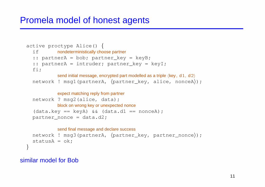
Promela model of honest agents

active proctype Alice() {if nondeterministically choose partner:: partnerA = bob; partner_key = keyB;:: partnerA = intruder; partner_key = keyI;fi;

send initial message, encrypted part modelled as a triple 〈key , d1, d2〉network ! msg1(partnerA, 〈partner_key, alice, nonceA 〉);

expect matching reply from partnernetwork ? msg2(alice, data);

block on wrong key or unexpected nonce(data.key == keyA) && (data.d1 == nonceA);partner_nonce = data.d2;

send final message and declare successnetwork ! msg3(partnerA, 〈partner_key, partner_nonce 〉);statusA = ok;

}

similar model for Bob

11

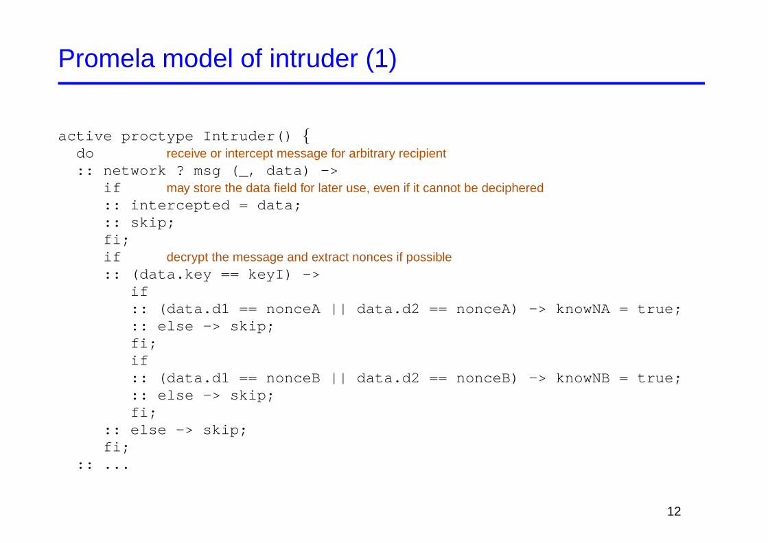
Promela model of intruder (1)

active proctype Intruder() {do receive or intercept message for arbitrary recipient:: network ? msg (_, data) ->

if may store the data field for later use, even if it cannot be deciphered:: intercepted = data;:: skip;fi;if decrypt the message and extract nonces if possible:: (data.key == keyI) ->

if:: (data.d1 == nonceA || data.d2 == nonceA) -> knowNA = true;:: else -> skip;fi;if:: (data.d1 == nonceB || data.d2 == nonceB) -> knowNB = true;:: else -> skip;fi;

:: else -> skip;fi;

:: ...

12

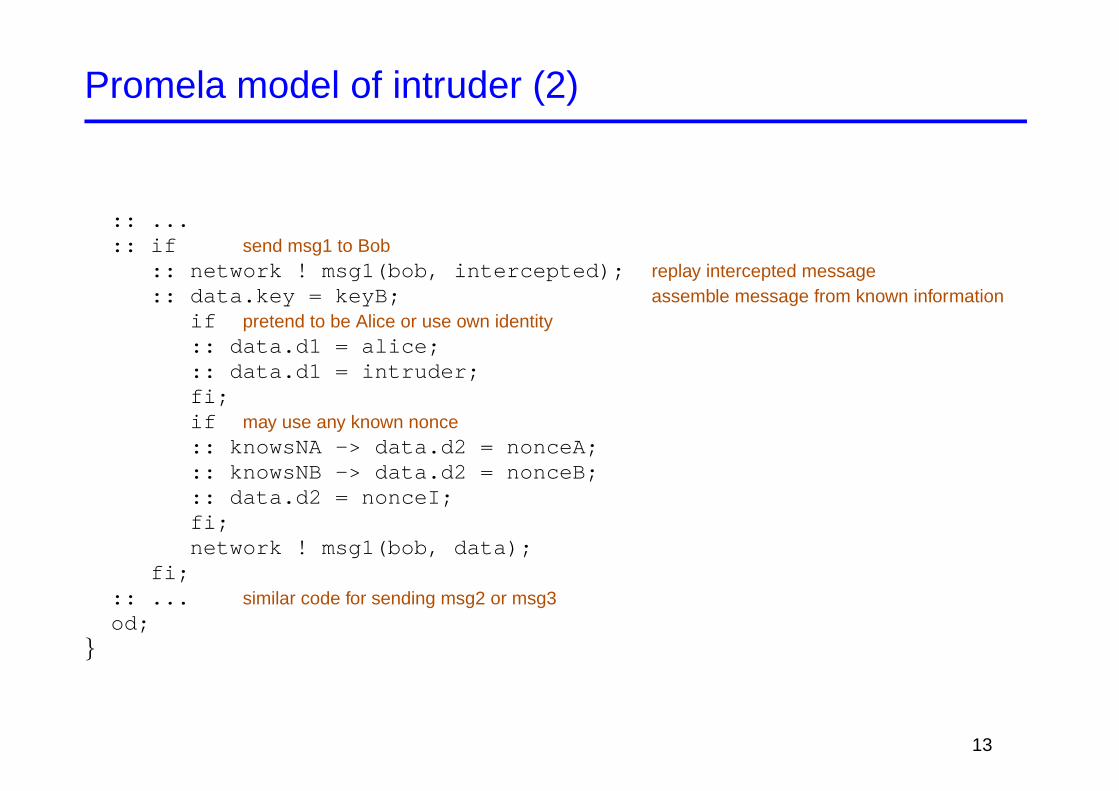
Promela model of intruder (2)

:: ...:: if send msg1 to Bob

:: network ! msg1(bob, intercepted); replay intercepted message:: data.key = keyB; assemble message from known information

if pretend to be Alice or use own identity:: data.d1 = alice;:: data.d1 = intruder;fi;if may use any known nonce:: knowsNA -> data.d2 = nonceA;:: knowsNB -> data.d2 = nonceB;:: data.d2 = nonceI;fi;network ! msg1(bob, data);

fi;:: ... similar code for sending msg2 or msg3od;

}

13

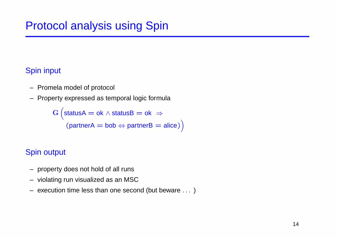
Protocol analysis using Spin

Spin input

– Promela model of protocol

– Property expressed as temporal logic formula

G(

statusA = ok ∧ statusB = ok ⇒

(partnerA = bob ⇔ partnerB = alice))

Spin output

– property does not hold of all runs

– violating run visualized as an MSC

– execution time less than one second (but beware . . . )

14

Protocol bug

Alice (correctly) believes to talk with Intruder

Bob (incorrectly) believes to talk with Alice

��AAA

��

Alice��AAA

��

Intruder��AAA

��

Bob

j

1 : 〈A,NA〉I

�4 : 〈NA,NB〉A

*

5 : 〈NB〉I

j

2 : 〈A,NA〉B

�3 : 〈NA,NB〉A

*

6 : 〈NB〉B

Bug went undetected for 17 years [Lowe, TACAS’96, LNCS 1055]

15

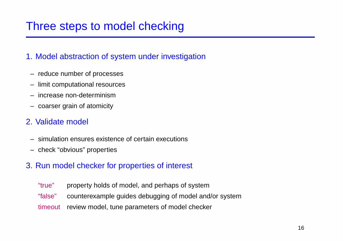
Three steps to model checking

1. Model abstraction of system under investigation

– reduce number of processes

– limit computational resources

– increase non-determinism

– coarser grain of atomicity

2. Validate model

– simulation ensures existence of certain executions

– check “obvious” properties

3. Run model checker for properties of interest

“true” property holds of model, and perhaps of system

“false” counterexample guides debugging of model and/or system

timeout review model, tune parameters of model checker

16

Kripke structures

Basic model of computation K = (S, I, δ,AP, L)

S system states (control, variables, channels)

I ⊆ S initial states

δ ⊆ S × S transition relation

AP atomic propositions over states

L : S → 2AP (labels) labelling function

All states assumed to have at least one successor

K described in modelling language (PROMELA, comm. automata, . . . )

Size of K usually exponential in size of description

Petri net view

S reachable markings

AP set of places

L(M) set of places marked at M

17

Example: Petri net

p1 p2

p3 p4 p5

p6

t1 t2 t3

t4 t5

t6

p7

t7

18

Example: Kripke structures

{p1,p2}

{p3,p2} {p1,p5} {p2,p4}

{p3,p5} {p4,p5}

{p6,p7}

{p1,p7} {p2,p6}

{p3,p7} {p4,p7} {p5,p6}

{I1,I2}

{N1,I2} {I1,N2} {N1,I2}

{N1,N2} {N1,N2}

{N1,N2}

{I1,N2} {N1,I2}

{N1,N2} {N1,N2} {N1,N2}

19

Computations of Kripke structures

Computations of K = (S, I, δ,AP, L)

infinite sequences L(s0)L(s1) . . . ∈ Sω satisfying s0 ∈ I and (si , si+1) ∈ δ

Petri net view

infinite sequences of markings M0M1 . . . starting at an initial marking and obeying the firingrule

Computation tree represents all computations of K

t

0

2

3

4

1 nodes system states

edges transitions

paths computations

branching non-determinism

(e.g., interleaving)

20

LTL: examples

Invariants G P

G¬(crit1 ∧ crit2) mutual exclusion

G(preset1 ∨ . . . ∨ presetn) deadlock freedom

Response, recurrence G(P ⇒ F Q)

G(try1 ⇒ F crit1) eventual access to critical section

G F¬crit1 no starvation in critical section

Reactivity, Streett G F P ⇒ G F Q

G F(try1 ∧ ¬crit2)⇒ G F crit1 strong fairness

Precedence G(P1 unless . . . unless Pn)

G(try1 ∧ try2 ⇒ ¬crit2 W crit2 W ¬crit2 W crit1) 1-bounded overtaking

22

Branching-time temporal logic

Include assertions about branching behavior

combine temporal modalities and quantification over paths

Example: CTL Computation Tree Logic

Q TXFGU, W

EA

for some pathsuccessor (next)

until, unlessfor all paths

sometime in the future (eventually)always in the future (globally)

evaluated at subtree K, s |= ϕ

system validity K |= ϕ iff K, s |= ϕ for all s ∈ I

Possibility properties

AG EF init home state, resettability

23

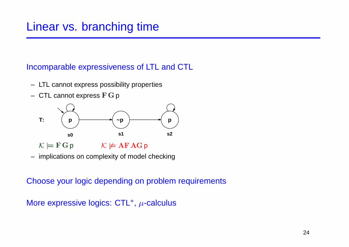
Linear vs. branching time

Incomparable expressiveness of LTL and CTL

– LTL cannot express possibility properties

– CTL cannot express F G p

p ~p p

s0 s1 s2

T:

K |= F G p K 6|= AF AG p

– implications on complexity of model checking

Choose your logic depending on problem requirements

More expressive logics: CTL∗, µ-calculus

24

Model-checking LTL I


25

Buchi automata

Finite automata operating on ω-words B = (Q, I, δ,F)

Q finite set of states

I ⊆ Q initial states

δ ⊆ Q ×Σ× Q transition relation

F ⊆ Q accepting states

same structure as finite automaton

Run of B on ω-word a0a1 . . . ∈ Σω

sequence q0a0−→ q1

a1−→ q2 · · ·

initialization q0 ∈ I

consecution (qi , ai , qi+1) ∈ δ for all i ∈ Naccepting qi ∈ F for infinitely many i ∈ N

ω-language defined by B

L(B) = {w ∈ Σω : B has some accepting run on w}ω-regular languages class of (ω-)languages definable by Buchi automata

26

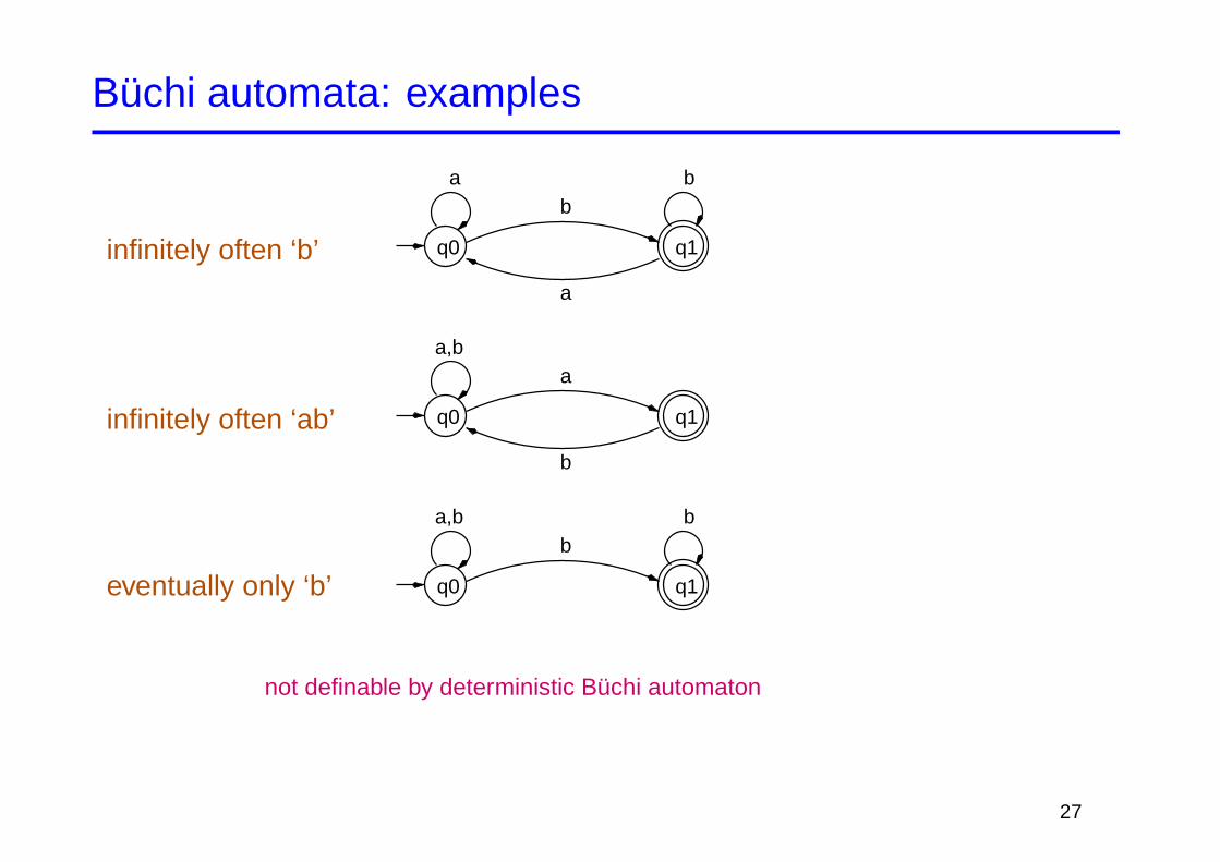
Buchi automata: examples

infinitely often ‘b’ q0 q1

ab

b

a

infinitely often ‘ab’ q0 q1

a,ba

b

eventually only ‘b’ q0 q1

bba,b

not definable by deterministic Buchi automaton

27

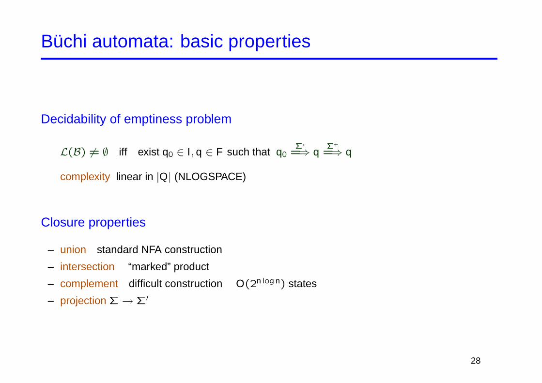
Buchi automata: basic properties

Decidability of emptiness problem

L(B) 6= ∅ iff exist q0 ∈ I, q ∈ F such that q0Σ∗

=⇒ qΣ+

=⇒ q

complexity linear in |Q| (NLOGSPACE)

Closure properties

– union standard NFA construction

– intersection “marked” product

– complement difficult construction O(2n log n) states

– projection Σ→ Σ′

28

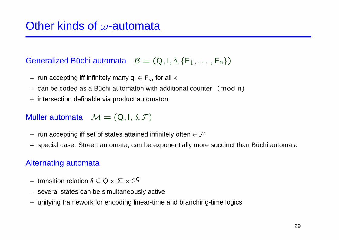
Other kinds of ω-automata

Generalized Buchi automata B = (Q, I, δ, {F1, . . . ,Fn})

– run accepting iff infinitely many qi ∈ Fk , for all k

– can be coded as a Buchi automaton with additional counter (mod n)

– intersection definable via product automaton

Muller automata M = (Q, I, δ,F)

– run accepting iff set of states attained infinitely often ∈ F– special case: Streett automata, can be exponentially more succinct than Buchi automata

Alternating automata

– transition relation δ ⊆ Q ×Σ× 2Q

– several states can be simultaneously active

– unifying framework for encoding linear-time and branching-time logics

29

From LTL to (generalized) Buchi automata

Basic insight

– Let L(ϕ) be the set of sequences of labels satisfying φ

– Construct automaton Bϕ recognizing L(ϕ) (alphabet of Bϕ is 2AP)

Idea of construction

states sets of subformulas of ϕ intended to be true at the next position

in the sequence of labels

initial states states containing ϕ

transition relation ensures satisfaction of non-temporal formulas in source state

replaces temporal formulas in source by others in target

temporal formulas decomposed according to recursion laws

Gϕ ≡ ϕ ∧X Gϕ

Fϕ ≡ ϕ ∨X Fϕ

ϕ until ψ ≡ ψ ∨ (ϕ ∧X(ϕ until ψ))

accepting states defined from “eventualities” Fϕ or ϕ until ψ

30

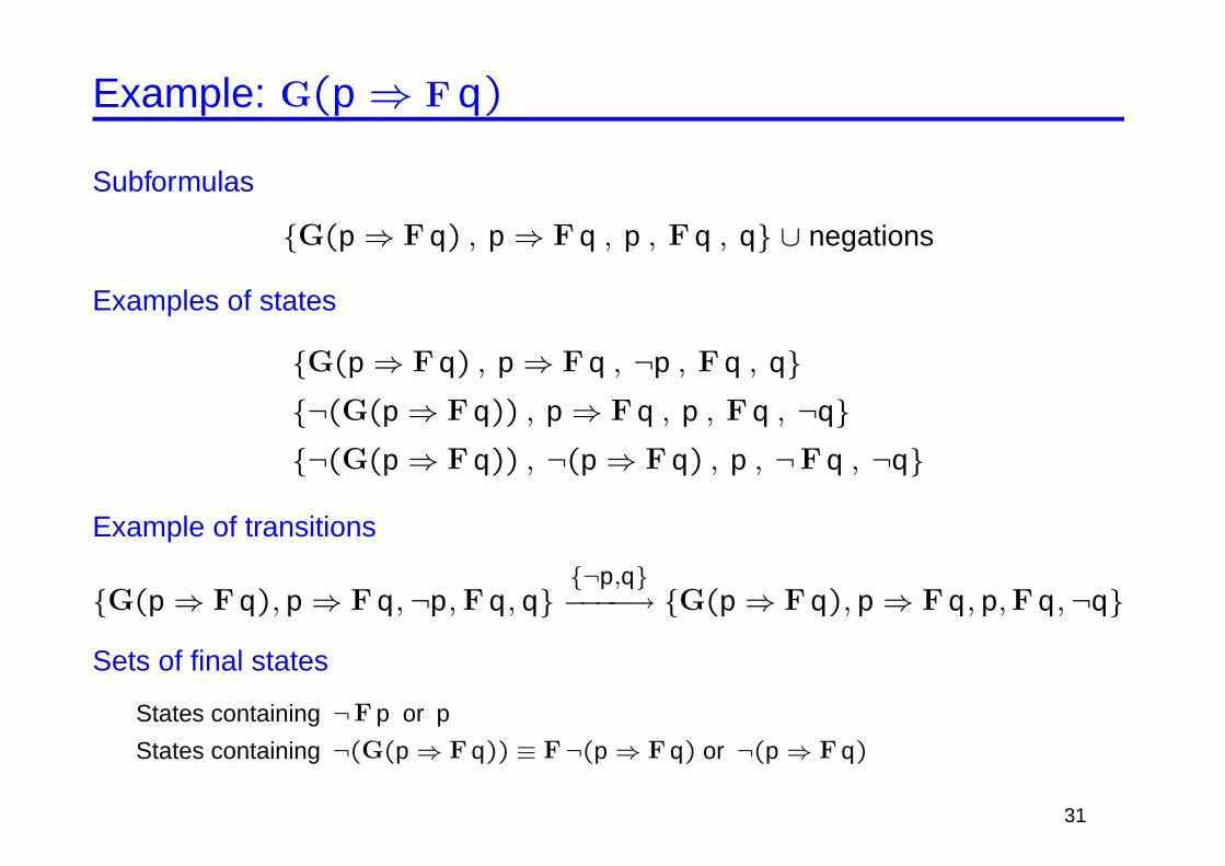
Example: G(p ⇒ F q)

Subformulas

{G(p ⇒ F q) , p ⇒ F q , p , F q , q} ∪ negations

Examples of states

{G(p ⇒ F q) , p ⇒ F q , ¬p , F q , q}{¬(G(p ⇒ F q)) , p ⇒ F q , p , F q , ¬q}{¬(G(p ⇒ F q)) , ¬(p ⇒ F q) , p , ¬F q , ¬q}

Example of transitions

{G(p ⇒ F q), p ⇒ F q,¬p,F q, q}{¬p,q}−−−−→ {G(p ⇒ F q), p ⇒ F q, p,F q,¬q}

Sets of final states

States containing ¬F p or p

States containing ¬(G(p ⇒ F q)) ≡ F¬(p ⇒ F q) or ¬(p ⇒ F q)

31

Result for the example (improved construction)

��&%'$

s0- &%'$

s1

R

p∧¬q

I

q

Y

¬q

¬p∨q

Complexity

– worst case: Bϕ exponential in length of ϕ

– improved constructions try to avoid exponential blow-up

Application LTL decision procedure

– ϕ satisfiable iff L(Bϕ) 6= ∅– exponential complexity (PSPACE)

32

Model Checking

Problem Given K and ϕ, decide whether K |= ϕ

Automata-theoretic solution

Consider K as ω-automaton with all states final

Define L(K) = set of computations of K

K |= ϕ

iff

L(K) ⊆ L(ϕ)

iff

L(K) ∩ L(¬ϕ) = ∅iff

L(K× B¬ϕ) = ∅

Complexity O(|K| · |B¬ϕ|) = O(|K| · 2|ϕ|)

33

State explosion

K× B¬ϕ is too big to be computed effectively

Problems start around 106 states

Solutions

– Reduce: ignore irrelevant portions of K× B¬ϕ– Compress: construct compact representation of K× B¬ϕ– Abstract: see section on abstraction

34

Model-checking LTL II

On-the-fly model checking

Partial-order techniques

35

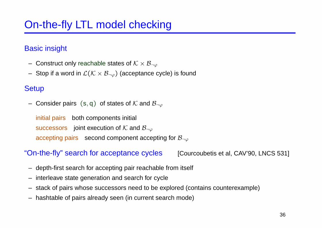
On-the-fly LTL model checking

Basic insight

– Construct only reachable states of K× B¬ϕ– Stop if a word in L(K× B¬ϕ) (acceptance cycle) is found

Setup

– Consider pairs (s, q) of states of K and B¬ϕ

initial pairs both components initial

successors joint execution of K and B¬ϕaccepting pairs second component accepting for B¬ϕ

“On-the-fly” search for acceptance cycles [Courcoubetis et al, CAV’90, LNCS 531]

– depth-first search for accepting pair reachable from itself

– interleave state generation and search for cycle

– stack of pairs whose successors need to be explored (contains counterexample)

– hashtable of pairs already seen (in current search mode)

36

On-the-fly LTL model checking

dfs(boolean search_cycle) {p = top(stack);foreach (q in successors(p)) {

if (search_cycle and (q == seed))report acceptance cycle and exit;

if ((q, search_cycle) not in visited) {enter (q, search_cycle) into visited;push q onto stack;dfs(search_cycle);if (not search_cycle and (q is accepting)) {

seed = q; dfs(true);} } }pop(stack);

}// initializationvisited = emptyset(); stack = emptystack(); seed = null;foreach initial pair p {

push p onto stack;enter (q, false) into visited;dfs(false)

}

37

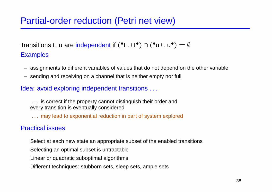
Partial-order reduction (Petri net view)

Transitions t , u are independent if (•t ∪ t•) ∩ (•u ∪ u•) = ∅Examples

– assignments to different variables of values that do not depend on the other variable

– sending and receiving on a channel that is neither empty nor full

Idea: avoid exploring independent transitions . . .

. . . is correct if the property cannot distinguish their order andevery transition is eventually considered

. . . may lead to exponential reduction in part of system explored

Practical issues

Select at each new state an appropriate subset of the enabled transitions

Selecting an optimal subset is untractable

Linear or quadratic suboptimal algorithms

Different techniques: stubborn sets, sleep sets, ample sets

38

Stubborn sets [Valmari, FMSD, 92]

A set U of transitions is stubborn at a marking M if

– for every t ∈ U, and every σ ∈ (T \ U)∗

Mσt−→ M ′ implies M

tσ−→ M ′

– either no transition is enabled at M, or there is t ∈ U such that for every σ ∈ (T \ U)∗

Mσ−→ implies M

σt−→ M ′

Reduced transition systems constructed using stubborn sets containall deadlock states and preserve existence of infinite paths

Efficiently constructing a stubborn set at a marking M:

– start with U = {t} for some t enabled at M

– if t ∈ U and t enabled, then add (•t)• (or •(•t)) to U

– if t ∈ U and t not enabled, then take p ∈ •t such that M(p) = 0 and add •p to U

More complicated definitions for preservation of LTL properties

39

Examples

p1 p2

p3 p4 p5

p6

t1 t2 t3

t4 t5

t6

p7

t7

{p1,p2}

{p1,p5}

{p3,p5} {p4,p5}

{p6,p7}

{p1,p7}

t3

t1 t2

t5t4

t6

t7

Deadlock freedom can be decided by exploring only six states

Needham-Schroeder: property checked by PROD after examining 942 states(out of 8279)

40

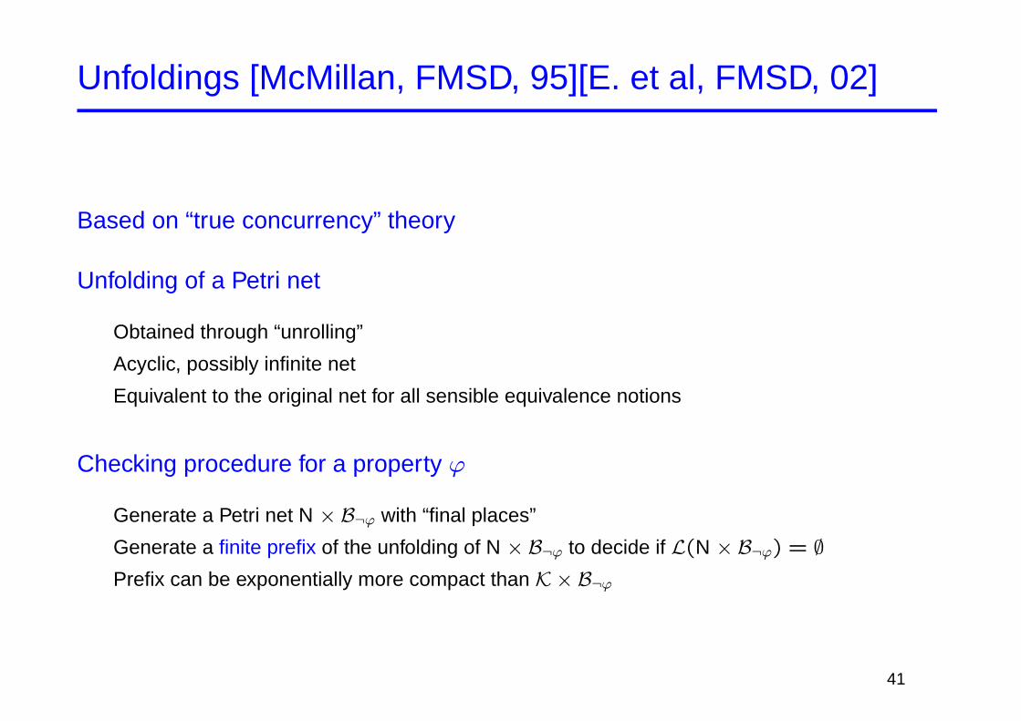
Unfoldings [McMillan, FMSD, 95][E. et al, FMSD, 02]

Based on “true concurrency” theory

Unfolding of a Petri net

Obtained through “unrolling”

Acyclic, possibly infinite net

Equivalent to the original net for all sensible equivalence notions

Checking procedure for a property ϕ

Generate a Petri net N × B¬ϕ with “final places”

Generate a finite prefix of the unfolding of N × B¬ϕ to decide if L(N × B¬ϕ) = ∅Prefix can be exponentially more compact than K× B¬ϕ

41

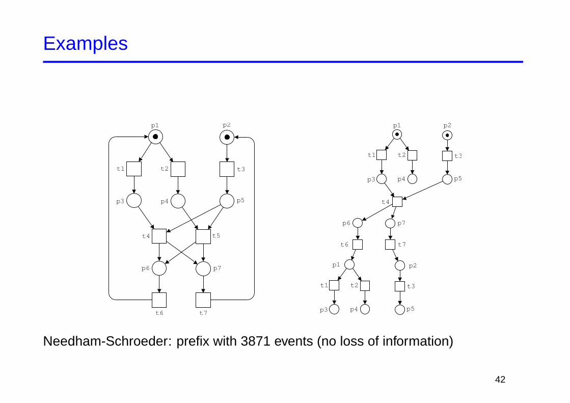
Examples

p1 p2

p3 p4 p5

p6

t1 t2 t3

t4 t5

t6

p7

t7

p1

p1

p2

p2

p3

p3

p4

p4

p5

p5

p6

t1

t1

t2

t2

t3

t3

t4

t6

p7

t7

Needham-Schroeder: prefix with 3871 events (no loss of information)

42

Model Checking CTL

Basic Algorithms

Binary Decision Diagrams

43

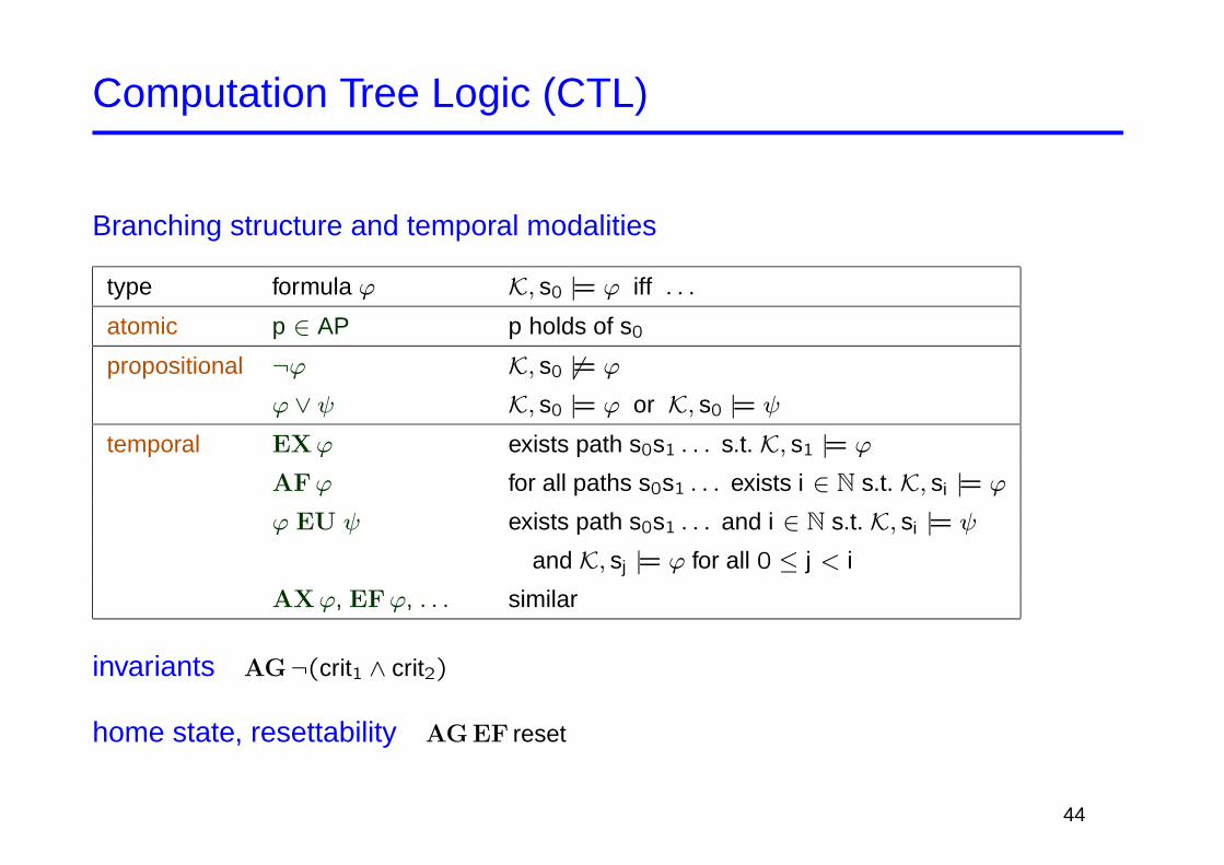
Computation Tree Logic (CTL)

Branching structure and temporal modalities

type formula ϕ K, s0 |= ϕ iff . . .

atomic p ∈ AP p holds of s0

propositional ¬ϕ K, s0 6|= ϕ

ϕ ∨ ψ K, s0 |= ϕ or K, s0 |= ψ

temporal EXϕ exists path s0s1 . . . s.t. K, s1 |= ϕ

AFϕ for all paths s0s1 . . . exists i ∈ N s.t. K, si |= ϕ

ϕ EU ψ exists path s0s1 . . . and i ∈ N s.t. K, si |= ψ

and K, sj |= ϕ for all 0 ≤ j < i

AXϕ, EFϕ, . . . similar

invariants AG¬(crit1 ∧ crit2)

home state, resettability AG EF reset

44

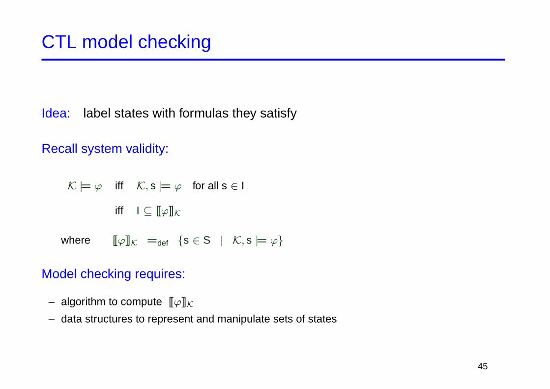
CTL model checking

Idea: label states with formulas they satisfy

Recall system validity:

K |= ϕ iff K, s |= ϕ for all s ∈ I

iff I ⊆ [[ϕ]]K

where [[ϕ]]K =def {s ∈ S | K, s |= ϕ}

Model checking requires:

– algorithm to compute [[ϕ]]K

– data structures to represent and manipulate sets of states

45

Bottom-up calculation of [[ϕ]]K

Observation: all CTL formulas definable from EX, EG, and EU, e.g.

AXϕ ≡ ¬EX¬ϕ EFϕ ≡ true EU ϕ

AGϕ ≡ ¬EF¬ϕ AFϕ ≡ ¬EG¬ϕ

simple cases: reformulation of CTL semantics

[[p]]K = {s ∈ S | p ∈ L(s)} for p ∈ AP

[[¬ψ]]K = S \ [[ψ]]K

[[ψ1 ∨ ψ2]]K = [[ψ1]]K ∪ [[ψ2]]K

[[EXψ]]K = δ−1([[ψ]]K) =def { s ∈ S | t ∈ [[ψ]]K for some t s.t. (s, t) ∈ δ }

missing cases: [[EGϕ]]K, [[ϕ EU ψ]]K

46

Calculation of [[EGϕ]]K

Observe recursion law

EGϕ ≡ ϕ ∧ EX EGϕ

In fact:

[[EGϕ]]K is the greatest “solution” of X = [[ϕ]]K ∩ δ−1(X) in (2S,⊆)

Proof.

– Recursion law implies that [[EGϕ]]K is a solution.

– Assume M = [[ϕ]]K ∩ δ−1(M) for M ⊆ S, show M ⊆ [[EGϕ]]K. Assume s0 ∈ M.

1. s0 ∈ [[ϕ]]K implies K, s0 |= ϕ.

2. s0 ∈ δ−1(M) implies there is s1 ∈ M s.t. (s0, s1) ∈ δ.Inductively obtain path s0, s1, . . . of states satisfying ϕ.

This proves K, s0 |= EGϕ and thus s0 ∈ [[EGϕ]]K.

47

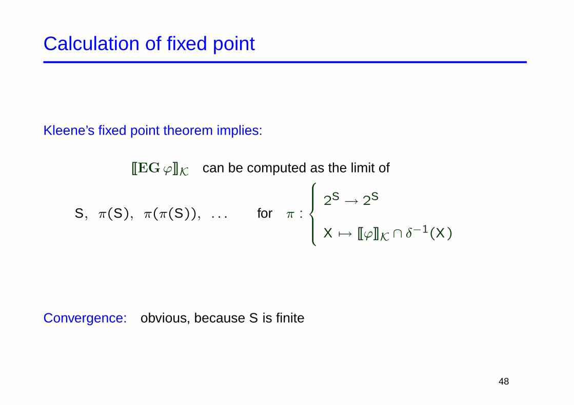
Calculation of fixed point

Kleene’s fixed point theorem implies:

[[EGϕ]]K can be computed as the limit of

S, π(S), π(π(S)), . . . for π :

2S → 2S

X 7→ [[ϕ]]K ∩ δ−1(X)

Convergence: obvious, because S is finite

48

Computation of greatest fixed point (1)

Compute [[EG y]]

x, y, z

s0

~x, y, ~z

~x, ~y, z

s6

x, ~y, ~z

s3

~x, ~y, ~z

s7

x, ~y, z

s5

x, y, ~z

s1s2

~x, y, z

s4

π0(S) = S

49


Compute [[EG y]]

x, y, z

s0

~x, y, ~z

s6

x, ~y, ~z

s3

~x, ~y, ~z

s7

x, ~y, z

s5

x, y, ~z

s1s2

~x, y, z

s4

~x, ~y, z

π1(S) = [[y]]K ∩ δ−1(S)

50


Compute [[EG y]]

x, y, z

s0

~x, y, ~z

s6

x, ~y, ~z

s3

~x, ~y, ~z

s7

x, ~y, z

s5

x, y, ~z

s1s2

~x, y, z

s4

~x, ~y, z

π2(S) = [[y]]K ∩ δ−1(π1(S))

51


Compute [[EG y]]

x, y, z

s0

~x, y, ~z

s6

x, ~y, ~z

s3

~x, ~y, ~z

s7

x, ~y, z

s5

x, y, ~z

s1s2

~x, y, z

s4

~x, ~y, z

π3(S) = [[y]]K ∩ δ−1(π2(S)) = π2(S): [[EG y]]K = {s0, s2, s4}

52

Calculation of [[ϕ EU ψ]]K

Similarly:

ϕ EU ψ ≡ ψ ∨ (ϕ ∧ EX(ϕ EU ψ))

[[ϕ EU ψ]]K is the smallest solution of X = [[ψ]]K ∪ ([[ϕ]]K ∩ δ−1(X))

Computation: calculate the limit of

∅, π(∅), π(π(∅)), . . . for π :

2S → 2S

X 7→ [[ψ]]K ∪ ([[ϕ]]K ∩ δ−1(X))

53

Computation of least fixed point (1)

Compute [[EF((x = z) ∧ (x 6= y))]]K

x, y, z

s0

~x, y, ~z

~x, ~y, z

s6

x, ~y, ~z

s3

~x, ~y, ~z

s7

x, ~y, z

s5

x, y, ~z

s1s2

~x, y, z

s4

π0(∅) = ∅

54


Compute [[EF((x = z) ∧ (x 6= y))]]

x, y, z

s0

~x, y, ~z

~x, ~y, z

s6

x, ~y, ~z

s3

~x, ~y, ~z

s7

x, ~y, z

s5

x, y, ~z

s1s2

~x, y, z

s4

π1(∅) = [[(x = z) ∧ (x 6= y)]]K ∪ δ−1(∅)

55



x, y, z

s0

~x, y, ~z

~x, ~y, z

s6

x, ~y, ~z

s3

~x, ~y, ~z

s7

x, ~y, z

s5

x, y, ~z

s1s2

~x, y, z

s4

π2(∅) = [[(x = z) ∧ (x 6= y)]]K ∪ δ−1(π1(∅))

56



x, y, z

s0

~x, y, ~z

~x, ~y, z

s6

x, ~y, ~z

s3

~x, ~y, ~z

s7

x, ~y, z

s5

x, y, ~z

s1s2

~x, y, z

s4

π3(∅) = [[(x = z) ∧ (x 6= y)]]K ∪ δ−1(π2(∅))

57



x, y, z

s0

~x, y, ~z

~x, ~y, z

s6

x, ~y, ~z

s3

~x, ~y, ~z

s7

x, ~y, z

s5

x, y, ~z

s1s2

~x, y, z

s4

π4(∅) = [[(x = z) ∧ (x 6= y)]]K ∪ δ−1(π3(∅)) = π3(∅):

[[EF((x = z) ∧ (x 6= y))]]K = {s4, s5, s6, s7}

58

Complexity issues

Complexity of fixed point algorithm: O(|ϕ| · |S| · (|S|+ |δ|))

Improved algorithm [Clarke et al, TOPLAS 8(2), 1986]

– Computation of [[EGϕ]]K

1. restrict K to states satisfying ϕ

2. compute SCCs of restricted graph

3. find states from which some SCC isreachable, using backward search

states satisfying ϕ

s |= EG ϕ

– Computation of [[ϕ EU ψ]]K can similarly be reduced to backward search

Complexity: O(|ϕ| · (|S|+ |δ|)) linear in size of model and formula

59

Fairness constraints

Recall limited expressiveness of CTL: fairness conditions not expressible

Instead: modify semantics and model checking algorithm

FairCTL: exclude “unfair” paths, e.g.

K, s0 |= EGfϕ iff there exists fair path s0, s1, . . . s.t. K, si |= ϕ for all i

K, s0 |= AGfϕ iff K, si |= ϕ holds for all fair paths s0, s1, . . . and all i

Fairness conditions specified by additional constraints

SMV: indicate CTL formulas that must hold infinitely often along a fair path

Key property: suffix closure

path s0, s1, s2, . . . is fair iff sn, sn+1, sn+2, . . . is fair (for all n)

60

Model checking FairCTL

Observe: EGf true holds at s iff there is some fair path from s

Suffix closure ensures

EXfϕ ≡ EX(ϕ ∧ EGf true )

ϕ EUf ψ ≡ ϕ EU (ψ ∧ EGf true )

Therefore: need only modify algorithm to compute [[EGfϕ]]K

assume k SMV-style fairness constraints: ψ1 ∧ . . . ∧ ψk

1. restrict K to states satisfying ϕ

2. compute SCCs of restricted graph

3. remove SCCs that do not contain a state satisfying ψj , for some j

4. [[EGfϕ]]K consists of states from which some (fair) SCC is reachable

Complexity: O(|ϕ| · (|S|+ |δ|) · k) still linear in the size of the model

61

Symbolic CTL model checking

Compress: data structures for model checking algorithm

compact representation of sets [[ϕ]]K ⊆ S and relation δ ⊆ S × S

Operations required

– Boolean operations on sets union, intersection, complement

– inverse image operation δ−1(M)

– comparison detect termination of fixed point computation

BDDs (binary decision diagrams) [Bryant, IEEE Trans. on Computers 33(2), 1986]

– widely used data structure for boolean functions

– compact, canonical dag representation of binary decision trees

– can represent large sets of regular structure

62

Compact set representations

Assume states are valuations of Boolean variables x0, x1, y0, y1

Example: set of states such that sum x1x0 ⊕ y1y0 produces carry

– explicit enumeration {x0x1y0y1, x0x1y0y1, x0x1y0y1, x0x1y0y1, x0x1y0y1, x0x1y0y1}– decision tree set elements correspond to paths leading to 1

– BDD dag obtained by removing redundant nodes and sharing equal subtrees

y1 y1 y1 y1 y1 y1 y1 y1

x0

x1

y0 y0 y0

x1

y0

0 0 0 0 0 1 0 1 0 0 0 1 0 1 1 1

0 1

0 1

0 1

0 1 0 1 0 1 0 1 0 1 0 1 0 1 0 1

0 1

0 1 0 01 1

;

x0

x1 x1

y0 y0

y1

1

0 1

1 0 1

01

1

1

63

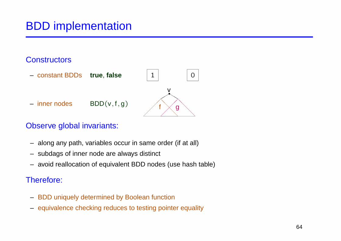
BDD implementation

Constructors

– constant BDDs true , false 1 0

– inner nodes BDD(v , f , g)

��

@@

@@@

f��

@@@@@

g

s"""bbb

v

Observe global invariants:

– along any path, variables occur in same order (if at all)

– subdags of inner node are always distinct

– avoid reallocation of equivalent BDD nodes (use hash table)

Therefore:

– BDD uniquely determined by Boolean function

– equivalence checking reduces to testing pointer equality

64

Boolean operations for BDDs

basic operation ite(f , g, h) = (f ∧ g) ∨ (¬f ∧ h) “if then else ”

all Boolean connectives definable from ite and constants

recursive computation

ite(true , g, h) = g ite(false , g, h) = h

Else: let v be “smallest” variable in f , g, h

ite(f , g, h) = v ∧ ite(f |v=true , g|v=true , h|v=true )

∨¬v ∧ ite(f |v=false , g|v=false , h|v=false )

=

{ite(f |v=true , . . . ) if ite(f |v=true , . . . ) = ite(f |v=false , . . . )

BDD(v , ite(f |v=true , . . . ), ite(f |v=false , . . . )) otherwise

Cofactor f |v=true , f |v=false for v at most head variable of f

equals left or right sub-dag of f if v is head variable, otherwise equals f

Complexity: O(|f | · |g| · |h|) if recomputation is avoided by hashing

65

BDD implementation: quantifiers

projection (∃x : ϕ) = (ϕ|x=true ∨ ϕ|x=false )

quantification over head variable

∃x : BDD(x , f , g)

= ∃x : (x ∧ f) ∨ (¬x ∧ g) [Def. BDD]

= (true ∧ f) ∨ (¬true ∧ g) ∨ (false ∧ f) ∨ (¬false ∧ g) [note: x does not occur in f ,g]

= f ∨ g

general case: quantification over several variables

∃x : BDD(y , f , g) =

{BDD(y , ∃x : f , ∃x : g) if y /∈ x

(∃x : f) ∨ (∃x : g) otherwise

universal quantification: similar

Complexity: worst case exponential, but usually works well in practice

66

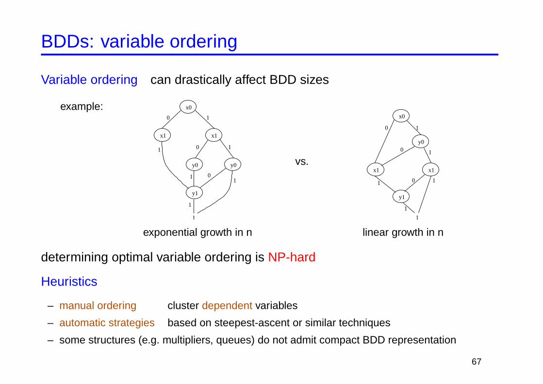
BDDs: variable ordering

Variable ordering can drastically affect BDD sizes

example: x0

x1 x1

y0 y0

y1

1

0 1

1 0 1

01

1

1

exponential growth in n

vs.

x0

y0

x1 x1

y1

1

0 1

0 1

1

1

0 1

linear growth in n

determining optimal variable ordering is NP-hard

Heuristics

– manual ordering cluster dependent variables

– automatic strategies based on steepest-ascent or similar techniques

– some structures (e.g. multipliers, queues) do not admit compact BDD representation

67

Symbolic CTL model checking: implementation

Symbolic representation

– state space S vector of (Boolean) state variables x

– initial states I BDD over x

– transition relation δ BDD over x,x′, perhaps split conjunctively

– sets [[ϕ]]K BDDs over x

Operations

– set operations Boolean operations on BDDs

– pre-image δ−1(M) = ∃x′ : δ ∧M ′

– set comparison pointer comparison

Complexity can be exponential in size of BDD representing δ

Results

– systems with huge potential state spaces (10many states) have been analysed

– particularly successful for synchronous hardware with short data paths

68

Infinite State Spaces

Sources of infinity

Symbolic search: forward and backward


69

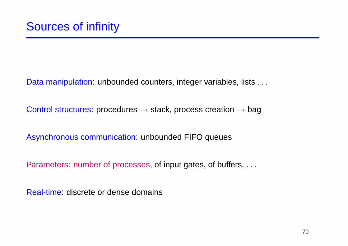
Sources of infinity

Data manipulation: unbounded counters, integer variables, lists . . .

Control structures: procedures→ stack, process creation→ bag

Asynchronous communication: unbounded FIFO queues

Parameters: number of processes, of input gates, of buffers, . . .

Real-time: discrete or dense domains

70

A bit of history

• Late 80s, early 90s: First theoretical papers

Decidability/Undecidability results for Place/Transition Petri nets

Efficient model-checking algorithms for context-free processes

Region construction for timed automata

• 90s: Research program

1. Decidability analysis

2. Design of algorithms or semi-algorithms

3. Design of implementations

4. Tools

5. Applications

• Late 90s, 00s: General techniques emerge

Automata-theoretic approach to model-checking

Symbolic reachability


71

Parametrized protocols

Defined for n processes.

Correctness: the desired properties hold for every n

Processes modelled as communicating finite automata

For each value of n the system has a finite state space (only one source ofinfinity)

Turing powerful, and so further restrictions sensible:

Broadcast Protocols

72

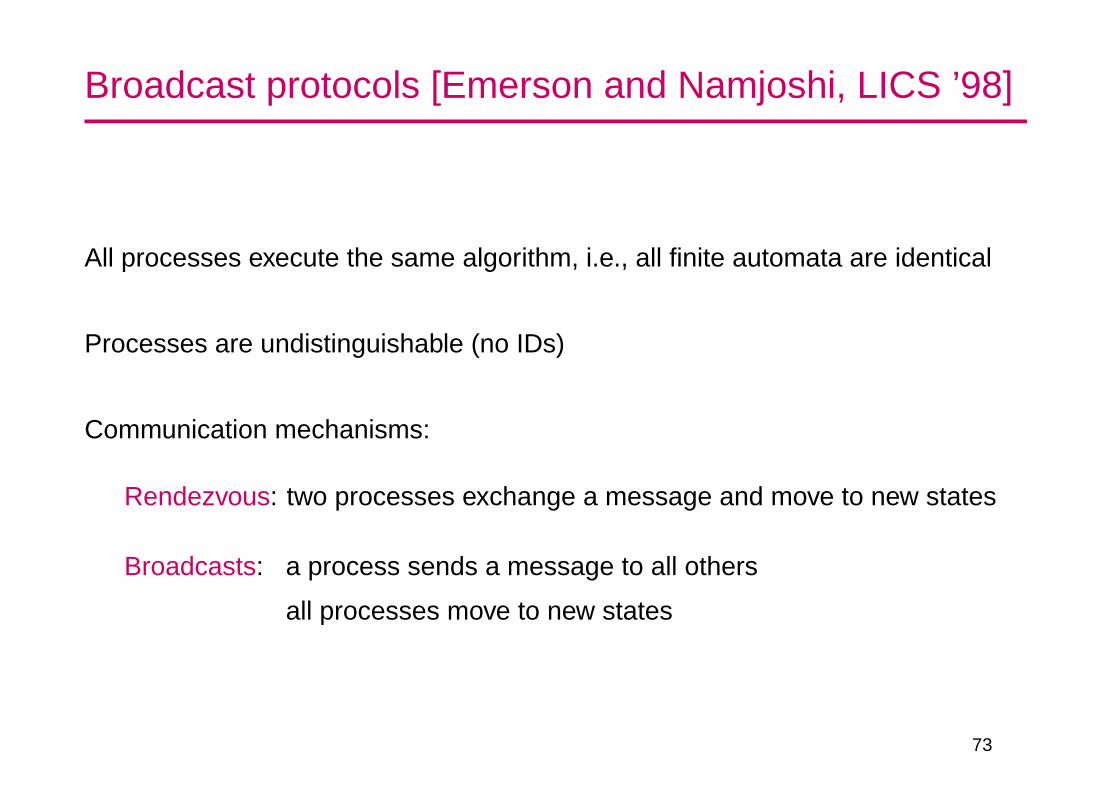
Broadcast protocols [Emerson and Namjoshi, LICS ’98]

All processes execute the same algorithm, i.e., all finite automata are identical

Processes are undistinguishable (no IDs)

Communication mechanisms:

Rendezvous: two processes exchange a message and move to new states

Broadcasts: a process sends a message to all others

all processes move to new states

73

Syntax

q3 q2

q1

a!!

a??

a??

a??

b!

b?

c

a!! : broadcast a message along (channel) aa??: receive a broadcasted message along ab! : send a message to one process along bb? : receive a message from one process along bc : change state without communicating with anybody

74

Semantics

The global state of a broadcast protocol is completelydetermined by the number of processes in each state.

Configuration: mapping : S → IN, seen as element of INn, where n = |S|Semantics for each n: finite transition system

– configurations as nodes

– channel names as transition labels

In our example:

(3,1,2)c−→ (4,0,2) (silent move)

(3,1,2)b−→ (3,2,1) (rendezvous)

(3,1,2)a−→ (2,1,3) (broadcast)

75

Semantics (continued)

Parametrized configuration: partial mapping p : Q → IN

– Intuition: “configuration with holes”

– Formally: set of configurations (total mappings matching p)

(Infinite) transition system of the broadcast protocol:

– Fix an initial parametrized configuration p0.

– Take the union of all finite transition systems Kc for each configuration c ∈ p0.

76

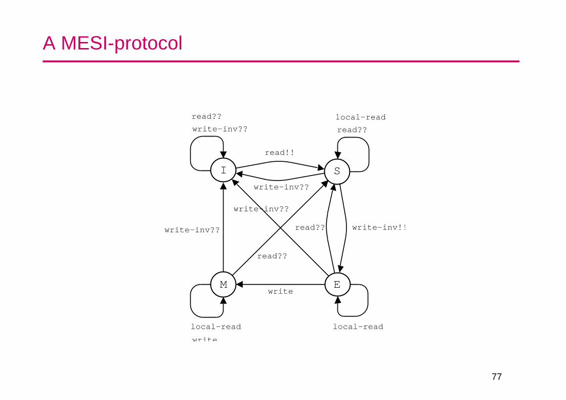
A MESI-protocol

read!!

write-inv!!

local-read

local-read

read??

read??

write

write

local-read

write-inv??

write-inv??

read??

write-inv??

write-inv??

read??

M E

SI

77


System S =⇒ Kripke structure K=⇒Languages L(K), Lω(K)

of finite and infinite computations

If systems closed under product with automata then B¬φ ×K=⇒S¬φ

Safety and liveness problems reducible to

– Reachability

Given: system S, sets I and F of initial and final configurations of KTo decide: if F can be reached from I, i.e., if there exist i ∈ I and f ∈ F such that i → f

– Repeated reachability

Given: System S, sets I and F of initial and final configurations of STo decide: if F can be repeatedly reached from I, i.e. if there exist i ∈ I and f1, f2, . . . ∈ Fsuch that i → f1 → f2 · · ·

Shape of I and F depend on the class of atomic propositions

78

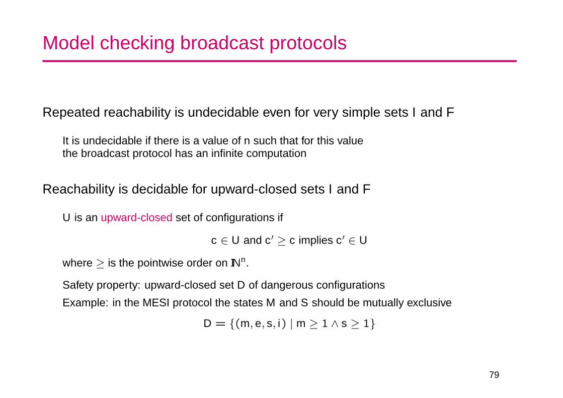
Model checking broadcast protocols

Repeated reachability is undecidable even for very simple sets I and F

It is undecidable if there is a value of n such that for this valuethe broadcast protocol has an infinite computation

Reachability is decidable for upward-closed sets I and F

U is an upward-closed set of configurations if

c ∈ U and c′ ≥ c implies c′ ∈ U

where ≥ is the pointwise order on INn.

Safety property: upward-closed set D of dangerous configurations

Example: in the MESI protocol the states M and S should be mutually exclusive

D = {(m, e, s, i) | m ≥ 1 ∧ s ≥ 1}

79

Symbolic search: forward and backward

Let C denote a (possibly infinite) set of configurations

Forward search

post(C) = immediate successors of C

Initialize C := I

Iterate C := C ∪ post(C) until

C ∩ F 6= ∅; return “reachable”, or

a fixpoint is reached; return “non-reachable”

Backward search

pre(C) = immediate predecessors of C

Initialize C := F

Iterate C := C ∪ pre(C) until

C ∩ I 6= ∅; return “reachable”, or

a fixpoint is reached; return “non-reachable”

Problem: when are the procedures effective?

80

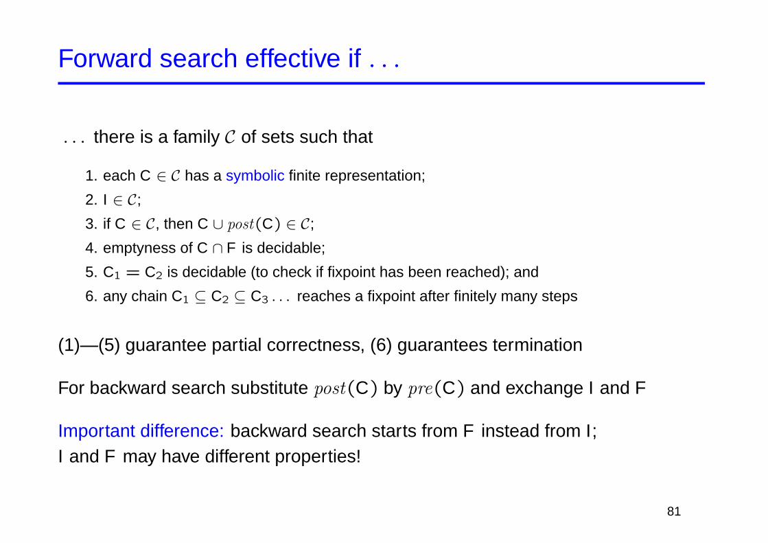
Forward search effective if . . .

. . . there is a family C of sets such that

1. each C ∈ C has a symbolic finite representation;

2. I ∈ C;

3. if C ∈ C, then C ∪ post(C) ∈ C;

4. emptyness of C ∩ F is decidable;

5. C1 = C2 is decidable (to check if fixpoint has been reached); and

6. any chain C1 ⊆ C2 ⊆ C3 . . . reaches a fixpoint after finitely many steps

(1)—(5) guarantee partial correctness, (6) guarantees termination

For backward search substitute post(C) by pre(C) and exchange I and F

Important difference: backward search starts from F instead from I;I and F may have different properties!

81

Forward search in broadcast protocols

C must contain all parametrized configurations.

Satisfies (1)—(5) but not (6). Termination fails in very simple cases.

q1 q2

a?? a??

a!!

(t,0)a−→ (t,1)

a−→ (t,2)a−→ . . .

82

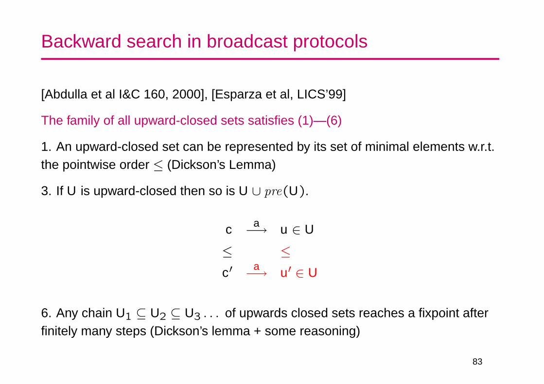
Backward search in broadcast protocols

[Abdulla et al I&C 160, 2000], [Esparza et al, LICS’99]

The family of all upward-closed sets satisfies (1)—(6)

1. An upward-closed set can be represented by its set of minimal elements w.r.t.the pointwise order ≤ (Dickson’s Lemma)

3. If U is upward-closed then so is U ∪ pre(U).

c a−→ u ∈ U

≤ ≤c′ a−→ u′ ∈ U

6. Any chain U1 ⊆ U2 ⊆ U3 . . . of upwards closed sets reaches a fixpoint afterfinitely many steps (Dickson’s lemma + some reasoning)

83

Application to the MESI-protocol

Are the states M and S mutually exclusive?

Check if the upward-closed set with minimal element

m = 1, e = 0, s = 1, i = 0

can be reached from the initial p-configuration

m = 0, e = 0, s = 0, i = t .

Proceed as follows:

U: m ≥ 1 ∧ s ≥ 1

U ∪ pre(U): (m ≥ 1 ∧ s ≥ 1) ∨(m = 0 ∧ e = 1 ∧ s ≥ 1)

U ∪ pre(U) ∪ pre2(U): U ∪ pre(U)

84

Other models

FIFO-automata with lossy channels

[Abdulla and Jonsson, I&C 127, 1993], [Abdulla et al, CAV’98, LNCS 1427]

Configuration: pair (q,w), where q state and w vector of words representing the queuecontents

Class C: upward-closed sets with the subsequence order

Backward search satisfies (1)—(6)

Timed automata

[Alur and Dill, TCS 126, 1994]

Configuration: pair (q,x), where q state and x vector of real numbers

Class C: regions

Forward search satisfies (1)—(6)

85

Implementing backwards reachability

Linear constraints as finite representation of sets of configurations.

The variable xi represents the number of processes in state qi

Set of configurations→ set of constraints over x = 〈x1, . . . , xn〉(interpreted disjunctively)

Immediate predecessors computed symbolically

Union and intersection −→ disjunction and conjunction

Containment test −→ entailment

86

Label a −→ linear transformation with guard.

In our example

• Guard Ga: x1 ≥ 1

• Linear transformation Max + ba:

Ma =

0 0 1

0 0 0

1 1 0

ba =

0

1

−1

Symbolic computation of pre must satisfy

pre(Φ) ≡∨

a∈Σ,φ∈Φ

Ga ∧ φ[x /Max + ba]

87

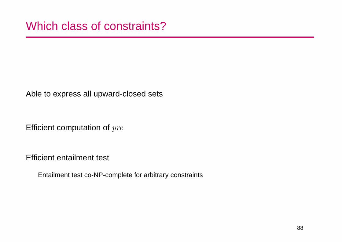
Which class of constraints?

Able to express all upward-closed sets

Efficient computation of pre

Efficient entailment test

Entailment test co-NP-complete for arbitrary constraints

88

Natural candidates

L-constraints

Conjunction of inequations of shape x1 + . . .+ xn ≥ c

Closed under broadcast transformations.

Entailment co-Np-complete even for single constraints

WA-constraints

Conjunction of inequations of shape xi ≥ c

Entailment is polynomial (quadratic)

Not closed under broadcast transformations.L-constraints equivalent to sets of WA-constraints, but with exponential blow-up:

xi1 + . . .+ xim ≥ c ≡∨

c1+...+cm=c

xi1 ≥ c1 ∧ xi2 ≥ c2 ∧ . . . ∧ xim ≥ cm

89

Using WA-constraints

[Delzanno and Raskin ’00]

Represent the constraint x1 ≥ c1 ∧ . . . ∧ xn ≥ cn by (c1, . . . cn)

Use sharing trees to represent sets of constraints

A sharing tree is an acyclic graph with one root and one terminal node such that

all nodes of layer i have successors in the layer i + 1

a node cannot have two successors with the same label

two nodes with the same label in the same layer do not have the same set of successors

90

A small Petri net experiment [Teruel ’98]

p1

p2

p3

p4

p5

p6

t1

t2

t3t6

p7

t5

t4

2 23

2

4

91

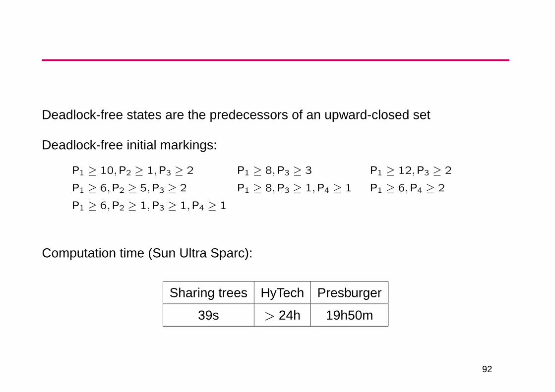
Deadlock-free states are the predecessors of an upward-closed set

Deadlock-free initial markings:

P1 ≥ 10,P2 ≥ 1,P3 ≥ 2 P1 ≥ 8,P3 ≥ 3 P1 ≥ 12,P3 ≥ 2

P1 ≥ 6,P2 ≥ 5,P3 ≥ 2 P1 ≥ 8,P3 ≥ 1,P4 ≥ 1 P1 ≥ 6,P4 ≥ 2

P1 ≥ 6,P2 ≥ 1,P3 ≥ 1,P4 ≥ 1

Computation time (Sun Ultra Sparc):

Sharing trees HyTech Presburger

39s > 24h 19h50m

92

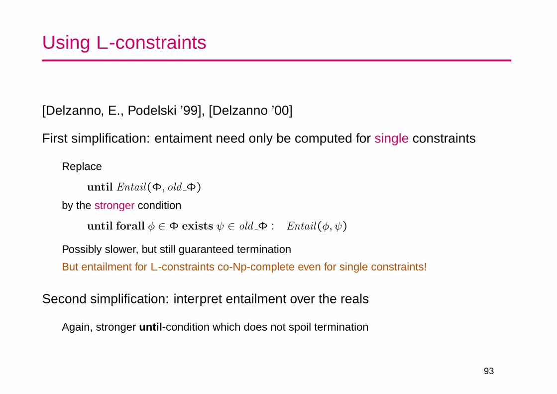
Using L-constraints

[Delzanno, E., Podelski ’99], [Delzanno ’00]

First simplification: entaiment need only be computed for single constraints

Replace

until Entail(Φ, old Φ)

by the stronger condition

until forall φ ∈ Φ exists ψ ∈ old Φ : Entail(φ, ψ)

Possibly slower, but still guaranteed termination

But entailment for L-constraints co-Np-complete even for single constraints!

Second simplification: interpret entailment over the reals

Again, stronger until -condition which does not spoil termination

93

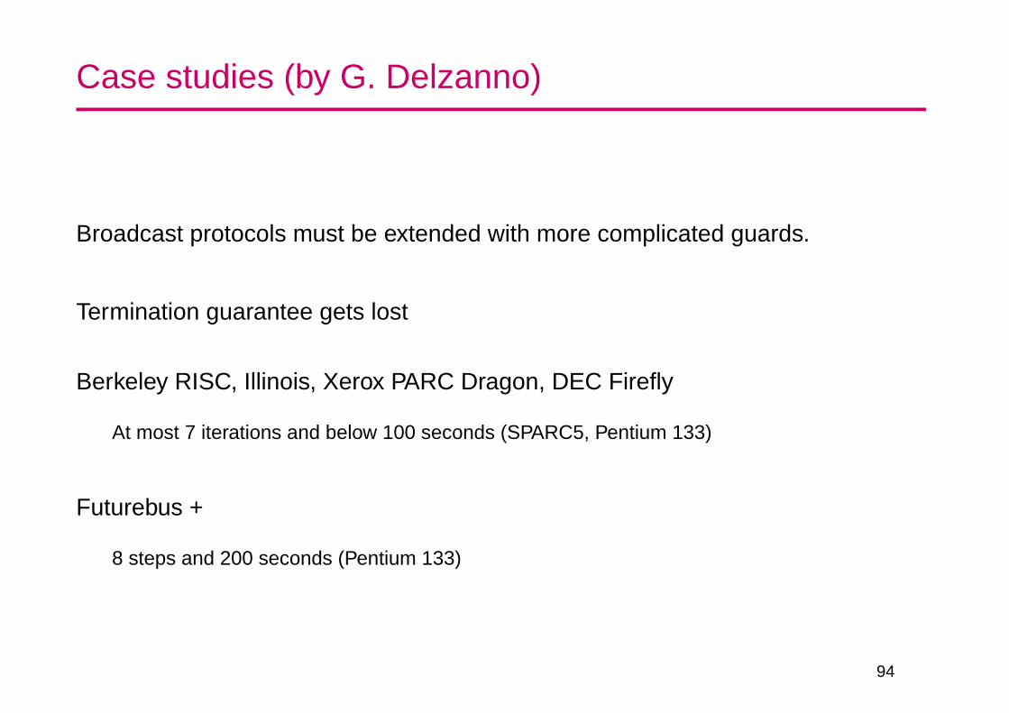
Case studies (by G. Delzanno)

Broadcast protocols must be extended with more complicated guards.

Termination guarantee gets lost

Berkeley RISC, Illinois, Xerox PARC Dragon, DEC Firefly

At most 7 iterations and below 100 seconds (SPARC5, Pentium 133)

Futurebus +

8 steps and 200 seconds (Pentium 133)

94

Accelerations and widenings: setup

post[σ](C) = set of configurations reached from C by the sequence σ

Compute a symbolic reachability graph with elements of C as nodes:

Add I as first node

For each node C and each label a, add an edge C a−→ post[a](C)

95

Accelerations

Replace C σ−→ post[σ](C) by C σ−→ X , where X satisfies

(1) post[σ](C) ⊆ X , and

(2) X contains only reachable configurations

Condition (1) guarantees the acceleration

Condition (2) guarantees that only reachable configurations are computed

96

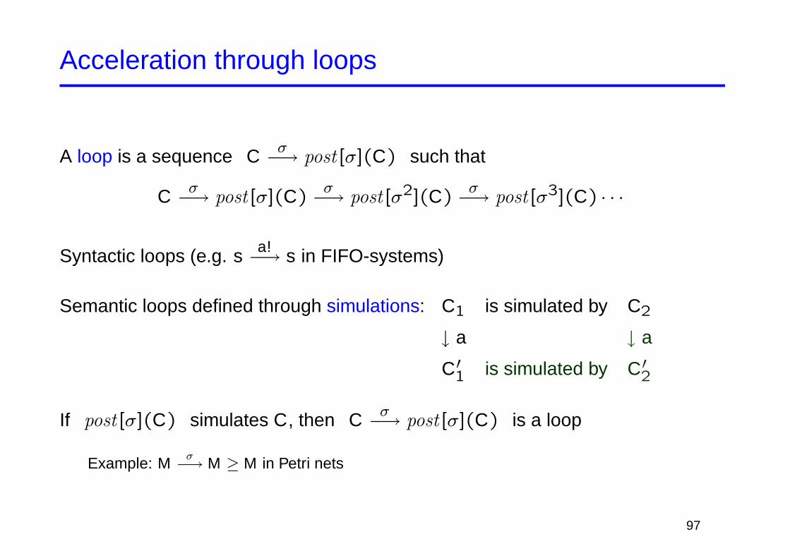
Acceleration through loops

A loop is a sequence C σ−→ post[σ](C) such that

C σ−→ post[σ](C)σ−→ post[σ2](C)

σ−→ post[σ3](C) · · ·

Syntactic loops (e.g. s a!−→ s in FIFO-systems)

Semantic loops defined through simulations: C1 is simulated by C2

↓ a ↓ a

C′1 is simulated by C′2

If post[σ](C) simulates C, then C σ−→ post[σ](C) is a loop

Example: Mσ−→ M ≥ M in Petri nets

97

Acceleration: given a loop C σ−→ post[σ](C) , replace post[σ](C) by

X = post[σ∗](C) = C ∪ post[σ](C) ∪ post[σ2](C) ∪ . . .

Problem: find a class of loops such that post[σ∗](C) belongs to C

98

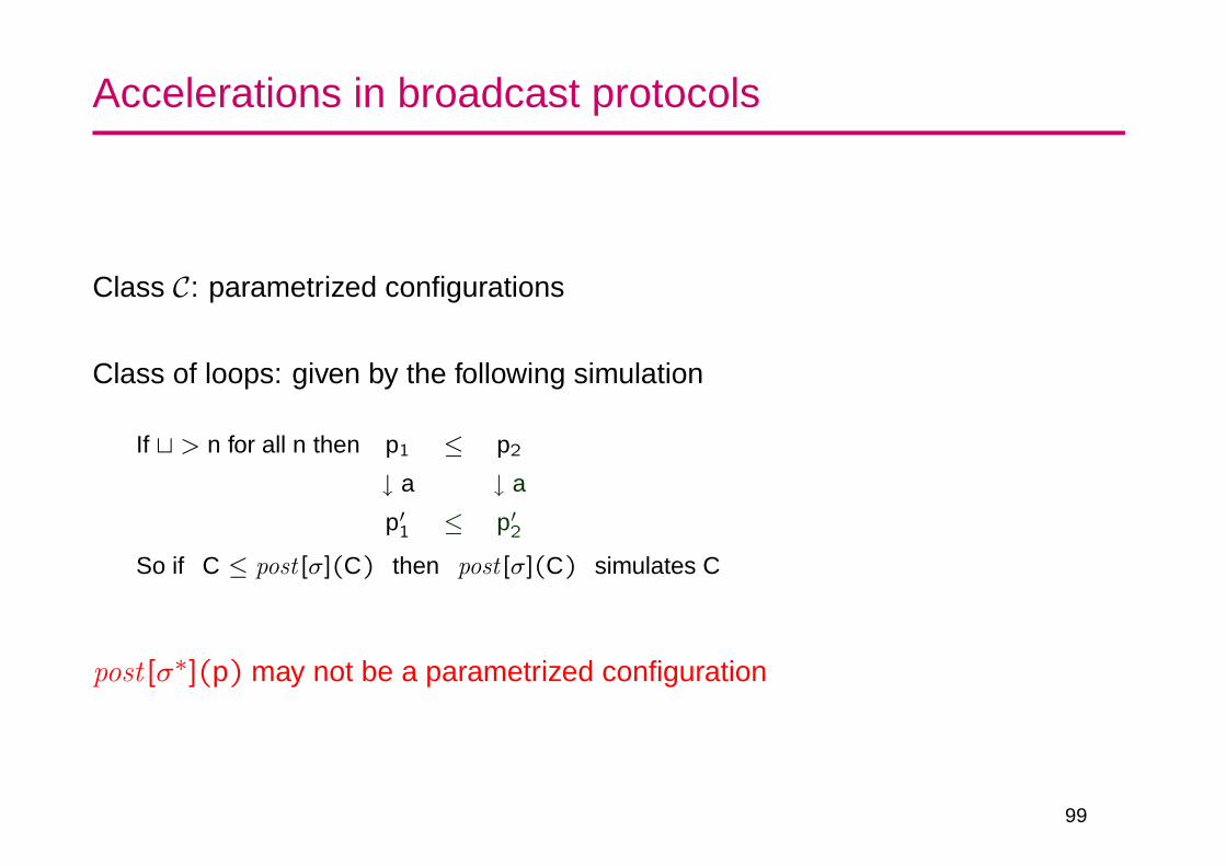
Accelerations in broadcast protocols

Class C: parametrized configurations

Class of loops: given by the following simulation

If t > n for all n then p1 ≤ p2

↓ a ↓ a

p′1 ≤ p′2

So if C ≤ post[σ](C) then post[σ](C) simulates C

post[σ∗](p) may not be a parametrized configuration

99

Other models I

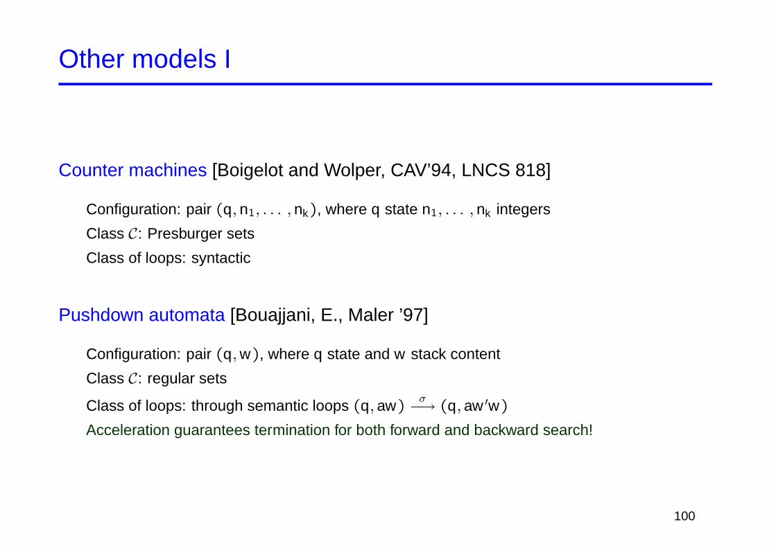
Counter machines [Boigelot and Wolper, CAV’94, LNCS 818]

Configuration: pair (q, n1, . . . , nk), where q state n1, . . . , nk integers

Class C: Presburger sets

Class of loops: syntactic

Pushdown automata [Bouajjani, E., Maler ’97]

Configuration: pair (q,w), where q state and w stack content

Class C: regular sets

Class of loops: through semantic loops (q, aw)σ−→ (q, aw ′w)

Acceleration guarantees termination for both forward and backward search!

100

Other models II

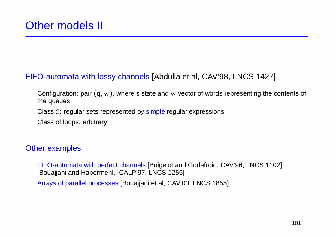
FIFO-automata with lossy channels [Abdulla et al, CAV’98, LNCS 1427]

Configuration: pair (q,w), where s state and w vector of words representing the contents ofthe queues

Class C: regular sets represented by simple regular expressions

Class of loops: arbitrary

Other examples

FIFO-automata with perfect channels [Boigelot and Godefroid, CAV’96, LNCS 1102],[Bouajjani and Habermehl, ICALP’97, LNCS 1256]

Arrays of parallel processes [Bouajjani et al, CAV’00, LNCS 1855]

101

Widenings

Accurate widenings

Replace Cσ−→ post[a](C) by C

σ−→ X , where X satisfies

(1) post[a](C) ⊆ X , and

(2’) X contains only reachable final configurations

Notice that X may contain unreachable non-final configurations!

Inaccurate widenings

Replace Cσ−→ post[a](C) by C

σ−→ X , where X satisfies

(1) post[a](C) ⊆ X

If no configuration of the graph belongs to F , then no reachable configuration belongs to F

If some configuration of the graph belongs to F , no information is gained

102

Accurate widenings in broadcast protocols

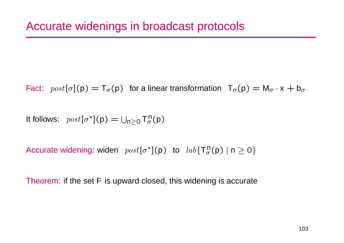
Fact: post[σ](p) = Tσ(p) for a linear transformation Tσ(p) = Mσ · x + bσ

It follows: post[σ∗](p) =⋃

n≥0 T nσ(p)

Accurate widening: widen post[σ∗](p) to lub{T nσ(p) | n ≥ 0}

Theorem: if the set F is upward closed, this widening is accurate

103

Does widening lead to termination?

For arbitrary broadcast protocols: NO [Esparza et al, LICS’99]

Example in which the acceleration doesn’t have any effect:

q1 q2 q3

a!!

a??

c

a??

p0 = (t,0,0)

For rendezvous communication only: YES[Karp and Miller ’69], [German and Sistla, JACM 39(3), 1992]

104

Conclusions

Decidability analysis very advanced

Many algorithms useful in practice

In the next years: improve implementations, integrate in tools.

Challenge: several sources of infinity.

105

Abstraction techniques

Basics

Predicate Abstraction

Extensions for liveness

106

State explosion problem

Exponential increase of reachable states with system size

Partial solutions

– reduce partial-order, symmetry: explore only relevant part of state space

– compress unfoldings, BDDs: efficient data structures

But: 10100 potential states are generated by just 300 bits

What about larger systems?

– hardware register files, execution pipelines

– software usually unbounded state size

Ad hoc approach

analyse small instances 2 cache lines, 3 potential data values, etc.

How do you make sure that you’ll catch the bug?

107

Abstraction

Idea

• compute “abstract system” K(finite, small)

• infer properties of Kfrom properties of K

Kj

s s

s K

��

AAAAAAA

K |= ϕ ⇐= K |= ϕ

Issues

– how to obtain and present abstract model?

– full automation or user interaction?

– what if K 6|= ϕ (“false negatives”) ?

Predicate abstraction: abstraction determined by predicates over concrete state space

– predicates of interest indicated by the user

– subsumes other abstraction techniques

– intuitive presentation of abstract model

108

Example: dining mathematicians

mutual exclusion for two processes (synchronization via integer variable n)

int n > 0loop

t0 : await even(n);

e0 : n := n div 2endloop

‖

loopt1 : await ¬even(n);

e1 : n := 3 ∗ n + 1endloop

abstract representation: control state, parity

'

&

$

%at e0, at t1

n > 0, even(n)

'

&

$

%at t0, at e1

n > 0, ¬even(n)

'

&

$

%at t0, at t1

n > 0, even(n)

'

&

$

%at t0, at t1

n > 0, ¬even(n)

? ?

?

6

?��*

HHHH

HHHH

HHH

HHH

HY

G(n > 0)

G¬(at e0 ∧ at e1)

G F at e0

G F at e1 can not be verified

109

Predicate diagrams [Bjorner et al, FMSD 16(3), 2000]

Fix set AP of atomic propositions

AP denotes set of propositions in AP and their negations

Presentation of abstraction as transition system A = (S, I, δ)

finite set S ⊆ 2AP of nodes (let s ∈ S also denote conjunction of literals)

Verification conditions for correctness of abstraction

– initialization: initial nodes of A cover initial states of K∨s∈I

s ⇒∨s∈I

L(s)

– consecution: transitions of A cover possible transitions of K

(s, t) ∈ δ if L(s)⇒ s and L(t)⇒ t for some (s, t) ∈ δ

Note: extra initial states or transitions preserves correctness

110

Preservation of properties

Correctness of abstraction implies:

– all computations of K represented as computations of A– properties of K can be inferred from those of A

A |= ϕ =⇒ K |= ϕ for all LTL (actually, ACTL∗) formulas ϕ over AP

– A |= ϕ established by model checking: consider atomic propositions as Boolean variables

A may contain additional computations

– A 6|= ϕ need not imply K 6|= ϕ

– counter example often suggests how to improve the abstraction

– spurious loops invalidate liveness properties (cf. “dining mathematicians”)

Strengthening abstractions

– split nodes extend set AP of atomic propositions

– break cycles represent information for liveness properties

111

Generating predicate diagrams (1)

Correct abstraction by elimination

– assume K being given by initial condition Init and transition relation Next

– start with full graph over 2AP

– remove node s from I if |= Init ⇒ ¬s

– remove edge (s, t) from δ if |= s ∧ Next ⇒ ¬t′

Implementation: use theorem prover

– try to prove implications using automatic tactic with limited resources

– many “local” goals instead of “global” property

– unproven implications: approximation, perhaps good enough

– drawback: 2|AP| states, 22|AP| proof attempts

Optimized implementation in PVS

Saıdi and Shankar, CAV’99, LNCS 1633

112

Generating predicate diagrams (2)

Compute abstraction by symbolic evaluation

– reduce: generate only reachable abstract states

– compilation approach: borrow from abstract interpretation

Formally: Galois connection

sets of states

α

zy

γ

Boolean algebra of predicates

Implementation

– rewrite s ∧ Next into disjunction t1′ ∨ . . . ∨ tn

′of successor states

– sample rules for “dining mathematicians”

even(x), even(y)⇒ even(x + y) even(x),¬even(y)⇒ ¬even(x + y)

x ∈ Nat , x > 0, even(x)⇒ x div 2 > 0 even(0) ¬even(1)

113

Example: bakery algorithm

Lamport’s mutual-exclusion protocol (2 processes, “atomic” version)

int t1 = 0, t2 = 0 (* “queueing tickets” *)loop

l1 : “noncritical section”;

l2 : t1 := t2 + 1;

l3 : await t2 = 0 ∨ t1 ≤ t2;

l4 : “critical section”;

l5 : t1 := 0endloop

‖

loopm1 : “noncritical section”;

m2 : t2 := t1 + 1;

m3 : await t1 = 0 ∨ ¬(t1 ≤ t2);

m4 : “critical section”;

m5 : t2 := 0endloop

Note: ticket values can grow arbitrarily large

Predicates of interest

– control state

– t1 = 0, t2 = 0, t1 ≤ t2

114

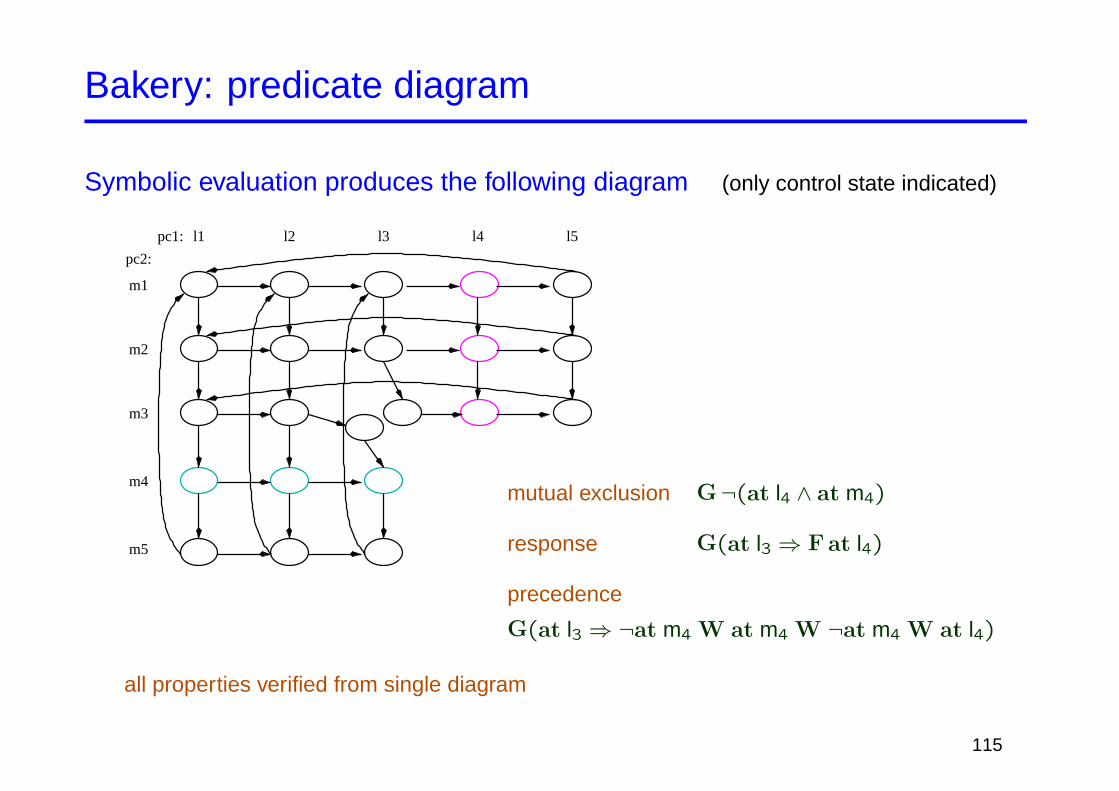
Bakery: predicate diagram

Symbolic evaluation produces the following diagram (only control state indicated)

l1 l3l2 l4 l5pc1:

pc2:

m1

m2

m3

m4

m5

mutual exclusion G¬(at l4 ∧ at m4)

response G(at l3 ⇒ F at l4)

precedence

G(at l3 ⇒ ¬at m4 W at m4 W ¬at m4 W at l4)

all properties verified from single diagram

115

Predicates on-the-fly

Symbolic evaluation can fail due to insufficient information

Bakery example: computing successors of

n =def {at l3, at m3, t1 6= 0, t2 6= 0}fails because guard g ≡ t1 ≤ t2 cannot be evaluated

Solution: reconsider predecessors of n

– for every predecessor m in the diagram, try to establish

m ∧ Next ∧ n′ ⇒

{g

¬g

}

– add (¬)g to the node label of n as appropriate

– possibly split node n

116

Predicates on-the-fly: Bakery example

'

&

$

%at l2, t1 = 0at m3, t2 6= 0

-

'

&

$

%at l3, t1 6= 0at m3, t2 6= 0

?

'

&

$

%at l3, t1 6= 0at m2, t2 = 0

;'

&

$

%at l2, t1 = 0at m3, t2 6= 0

?'

&

$

%

at l3, t1 6= 0at m3, t2 6= 0¬(t1 ≤ t2)

'

&

$

%at l3, t1 6= 0at m3, t2 6= 0

t1 ≤ t2

-

'

&

$

%at l3, t1 6= 0at m2, t2 = 0

Predicate t1 ≤ t2 need not be supplied by the user

inferred predicates added precisely where necessary

117

Strengthening for liveness

Boolean abstractions often cannot prove liveness properties

– predicate diagram usually contains cycles that do not correspond to “concrete” computations

– “dining mathematicians” example: liveness for process 1 could not be verified

Standard techniques to establish liveness properties

– fairness conditions action taken infinitely often if sufficiently often enabled

– well-founded orderings exclude cycles that correspond to infinite descent

These need to be represented in the abstraction!

118

Representing fairness conditions

Annotate (some) transitions in δ with actions A ∈ Act

– formally, transitions are now triples δ ⊆ S × Act × S

– assume actions are described by characteristic predicate over (x,x′)

Correctness conditions (s,A, t) ∈ δ implies:

– enabledness: action A is enabled at s

s ⇒ ∃x′ : A

– effect: represent all possible A-successors

s ∧ A⇒∨

(s,A,t)∈δ

t′

119

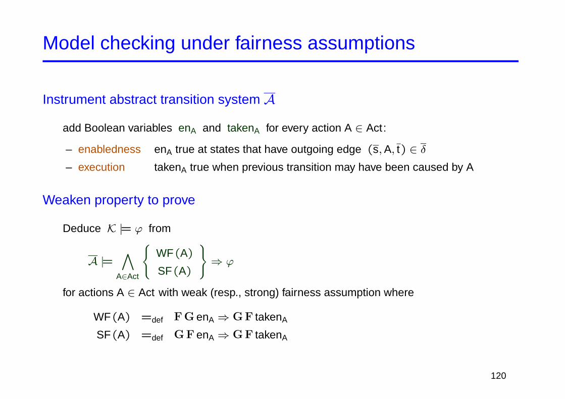
Model checking under fairness assumptions

Instrument abstract transition system A

add Boolean variables enA and takenA for every action A ∈ Act :

– enabledness enA true at states that have outgoing edge (s,A, t) ∈ δ– execution takenA true when previous transition may have been caused by A

Weaken property to prove

Deduce K |= ϕ from

A |=∧

A∈Act

{WF(A)

SF(A)

}⇒ ϕ

for actions A ∈ Act with weak (resp., strong) fairness assumption where

WF(A) =def F G enA ⇒ G F takenA

SF(A) =def G F enA ⇒ G F takenA

120

Representing well-founded orderings

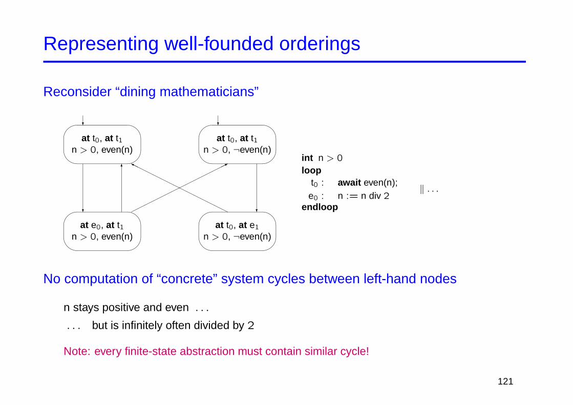
Reconsider “dining mathematicians”

'

&

$

%at e0, at t1

n > 0, even(n)

'

&

$

%at t0, at e1

n > 0, ¬even(n)

'

&

$

%at t0, at t1

n > 0, even(n)

'

&

$

%at t0, at t1

n > 0, ¬even(n)

? ?

?

6

?��*

HHHHH

HHH

HHH

HHHHY

int n > 0

loopt0 : await even(n);

e0 : n := n div 2endloop

‖ . . .

No computation of “concrete” system cycles between left-hand nodes

n stays positive and even . . .

. . . but is infinitely often divided by 2

Note: every finite-state abstraction must contain similar cycle!

121

Ordering annotations

Represent descent w.r.t. well-founded ordering in A

– let t be (concrete-level) term and ≺ be well-founded ordering on domain of t

– label edge (m,A, n) ∈ δ by (t ,≺) (resp., (t ,�)) if

m ∧ A ∧ n′ ⇒

{t ′ ≺ t

t ′ � t

}

Use edge annotations in model checking

– exclude computations of A that correspond to infinite descent of t in K:

Deduce K |= ϕ from A |= (G F “t ′ ≺ t”⇒ G F¬“t ′ � t”) ⇒ ϕ

– “t ′ ≺ t” represented by auxiliary Boolean variables

122

Dining mathematicians completed

Diagram annotated with ordering information

'

&

$

%at e0, at t1

n > 0, even(n)

'

&

$

%at t0, at e1

n > 0, ¬even(n)

'

&

$

%at t0, at t1

n > 0, even(n)

'

&

$

%at t0, at t1

n > 0, ¬even(n)

? ?

?

(n,≤)

6

(n, <)

?��*

HHHHH

HHH

HHHH

HHHY

G(n > 0)

G¬(at e0 ∧ at e1)

G F at e0

G F at e1 can not be verified��HHH

G F at e1 can also

Justification

– at t0 ∧ even(n) ∧ Next ⇒ n′ = n

– at e0 ∧ even(n) ∧ n > 0 ∧ Next ⇒ n′ = n div 2

123

Summary

Semi-automatic construction of abstraction followed by model checking

Combination of model checking, theorem proving, and abstract interpretation

Challenge: integrate tools (SAL project at SRI, Stanford, Berkeley, Grenoble)

Identify useful abstractions that can be generated automatically

Parameterized systems [Manna and Sipma, CAV’99, LNCS 1663];[Baukus et al,TACAS’00, LNCS 1785]

124

Model Checking - TUM - Chair VII - Foundations of …esparza/Talks/slides-maratea.pdf · Model...

Documents

Transcript of Model Checking - TUM - Chair VII - Foundations of …esparza/Talks/slides-maratea.pdf · Model...