Model calibration of a vehicle tailgate using...
100
Department of Applied Mechanics Division of Dynamics CHALMERS UNIVERSITY OF TECHNOLOGY Gothenburg, Sweden 2015 Master’s Thesis 2015:26 Model calibration of a vehicle tailgate using frequency response functions Master’s thesis in Applied Mechanics IÑIGO ECHANIZ GRANADO
Transcript of Model calibration of a vehicle tailgate using...
Department of Applied Mechanics
Division of Dynamics
CHALMERS UNIVERSITY OF TECHNOLOGY
Gothenburg, Sweden 2015
Master’s Thesis 2015:26
Model calibration of a vehicle tailgate using frequency response functions
Master’s thesis in Applied Mechanics
IÑIGO ECHANIZ GRANADO


MASTER’S THESIS IN APPLIED MECHANICS
Model calibration of a vehicle tailgate using frequency
response functions
IÑIGO ECHANIZ GRANADO
Department of Applied Mechanics
Division of Dynamics
CHALMERS UNIVERSITY OF TECHNOLOGY
Göteborg, Sweden 2015

Model calibration of a vehicle tailgate using frequency response functions
IÑIGO ECHANIZ GRANADO
© IÑIGO ECHANIZ GRANADO, 2015-01-01
Master’s Thesis 2015:26
ISSN 1652-8557
Department of Applied Mechanics
Division of Dynamics
Chalmers University of Technology
SE-412 96 Göteborg
Sweden
Telephone: + 46 (0)31-772 1000
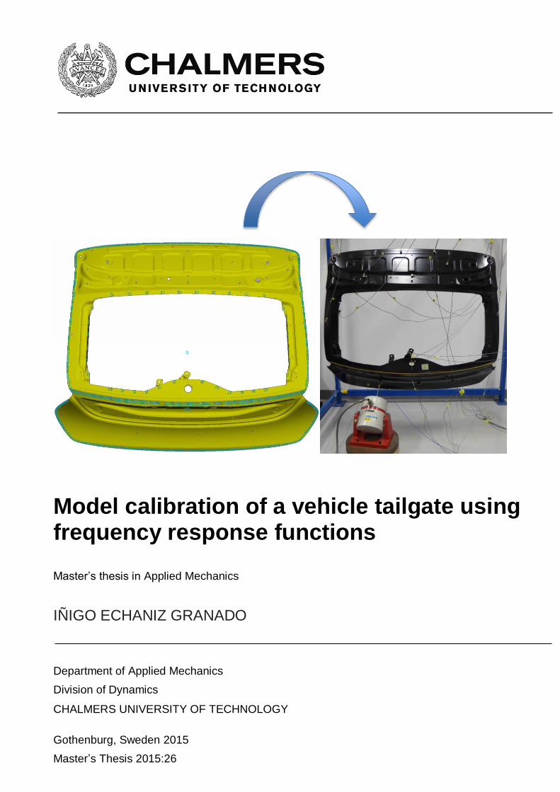
Cover:
The finite element model of the tailgate shown in the left part of the figure is
calibrated employing test data obtained from measuring the real tailgate in the right
part of the figure.
Chalmers Reproservice / Department of Applied Mechanics
Göteborg, Sweden 2015-01-01


I
Model calibration of a vehicle tailgate using frequency response functions
Master’s thesis in Applied Mechanics
IÑIGO ECHANIZ GRANADO
Department of Applied Mechanics
Division of Dynamics
Chalmers University of Technology
Abstract
This thesis is dedicated to calibrate the FE-model of the Volvo V40 vehicle tailgate in
order to derive modelling guidelines for future applications. The calibration is
conducted against data obtained from vibration testing employing an optimisation
algorithm based on the minimisation of the deviation metric between the frequency
response functions. A pre-test planning is conducted to ensure the observability and
controllability of the target modes during the experiments. Three different tailgates
are measured utilising two types of signals to excite the system: stepped-sine
excitation and burst-random excitation. Small differences are observed comparing the
results according to the excitation strategies. Stepped-sine testing is believed to be
more accurate, as the steady state condition of the system is ensured. Even if the
measured objects are simple, dispersion is found between the tailgates, mainly at high
frequencies. A state-space model is established using system identification on one of
the tested objects. Model calibration is performed on the FE-model based on the
identified model. The calibrated model is found to predict the dynamics of the system
in great correlation with the test data, thus the nominal model is significantly
improved. Conclusions in modelling guidelines are drawn from the calibrated model;
mapping the thickness corresponding to simulations on metal forming into the parts of
the numerical model, together with modifying the properties of the adhesive such that
the stiffness corresponds to steel and the Poisson’s ratio corresponds to
incompressible material, substantially increases the prediction capability of the model.
Slightly lowering the stiffness and density of the metal parts while slightly reducing
the stiffness of the shell elements around the welded parts, employed to represent the
spot weld connections, improves the curve fitting between the numerical model and
the test data. In conclusion, the metal parts composing the model are improved with
mapping of the thickness and modification of their properties. The connections
between the parts of the model are also improved by changing the properties of the
adhesive to mimic the real seaming effect and with the stiffness adjustment of the
shell elements around welds.
Key words: Frequency response function, vibration testing, stepped-sine excitation,
burst-random excitation, tailgate, system identification, calibration, seaming
modelling guidelines.

II
III
Contents
Abstract .................................................................................................................. I
Contents .............................................................................................................. III
Preface ............................................................................................................... VII
Acknowledgements ............................................................................................ VII
Acronyms .......................................................................................................... VIII
1 Introduction ....................................................................................................... 1
1.1 Background ................................................................................................. 1
1.2 Goal ............................................................................................................ 1
1.3 Problem description ..................................................................................... 1
1.4 Method ........................................................................................................ 1
1.5 Limitations .................................................................................................. 2
2 Theory ............................................................................................................... 3
2.1 Important definitions ................................................................................... 3
2.1.1 Model verification ................................................................................ 3
2.1.2 Model validation .................................................................................. 3
2.1.3 Model calibration ................................................................................. 3
2.2 Basics of structural dynamics ...................................................................... 4
2.2.1 Linear model ........................................................................................ 4
2.2.2 State-space model................................................................................. 4
2.2.3 Model reduction ................................................................................... 4
2.2.4 Frequency response function ................................................................ 5
2.3 FE-modelling of connections in VCC .......................................................... 5
2.3.1 Modelling of spot welds ....................................................................... 5
2.3.2 Modelling of adhesive .......................................................................... 6
2.3.3 Modelling of screws ............................................................................. 6
2.3.4 Rbe2 and rbe3 connections ................................................................... 7
2.4 Pre-test planning.......................................................................................... 7
2.4.1 Method of effective independence ........................................................ 7
2.4.2 Observability and controllability .......................................................... 8
2.5 Testing ........................................................................................................ 9
2.5.1 Vibration testing hardware ................................................................... 9
2.5.2 Set-up of the experiments ................................................................... 11

IV
2.5.3 System excitation ............................................................................... 12
2.5.4 Signal processing ............................................................................... 13
2.6 System identification ................................................................................. 13
2.7 Correlation indicators ................................................................................ 13
2.7.1 Modal Assurance Criterion ................................................................. 14
2.7.2 Deviation metric ................................................................................. 14
2.8 Model calibration using FEMcali............................................................... 15
2.8.1 FEMcali working procedure ............................................................... 16
3 FE-model of the tailgate ................................................................................... 18
3.1 Parameters in the FE-model ....................................................................... 20
4 Testing process ................................................................................................ 21
4.1 Pre-test planning........................................................................................ 21
4.1.1 Observability and controllability ........................................................ 22
4.2 Testing the tailgates ................................................................................... 24
4.2.1 Testing software ................................................................................. 24
4.2.2 Testing hardware ................................................................................ 24
4.2.3 Set-up of testing ................................................................................. 27
4.2.4 Optimising data acquisition ................................................................ 30
4.2.5 System excitation ............................................................................... 34
4.3 Results from measurements ....................................................................... 38
4.3.1 Mass of tested tailgates ....................................................................... 38
4.3.2 Dispersion between testing objects ..................................................... 38
4.3.3 Differences between excitation strategies ........................................... 41
5 FE-model vs test data ....................................................................................... 44
5.1 System identification on test data .............................................................. 44
5.1.1 Remove influence from bungee-cords ................................................ 44
5.1.2 Mobility data ...................................................................................... 44
5.1.3 Frequency response data object .......................................................... 45
5.1.4 Model order estimation....................................................................... 45
5.1.5 State-space model inflation................................................................. 47
5.1.6 State-space model vs raw test data ...................................................... 48
5.2 Evaluation of testing results ....................................................................... 49
5.3 FE-model updating .................................................................................... 50
5.3.1 Mapping of thickness ......................................................................... 50
V
5.3.2 Seaming effect ................................................................................... 53
5.4 Calibration using FEMcali ......................................................................... 57
6 Results and Discussion .................................................................................... 62
6.1 Nominal vs calibrated FE-model ............................................................... 62
6.2 Derived modelling guidelines .................................................................... 66
7 Conclusions ..................................................................................................... 68
8 Future Work .................................................................................................... 71
9 References ....................................................................................................... 72
Appendix A Testing............................................................................................... i
Appendix B Test Results ..................................................................................... iii
Appendix C Mapped thickness .......................................................................... viii
Appendix D FE-model vs test data ....................................................................... ix

VI
VII
Preface
In this thesis, model calibration of a vehicle tailgate has been accomplished in order to
derive modelling guidelines for future applications. The calibration of the finite
element model has been conducted against test data. The experiments were performed
in the labs at Volvo Car Corporation. The project has been conducted during 20
weeks, from January to June 2015.
The work is part of a method development project to derive guidelines seeking for
modelling techniques that will improve the prediction capabilities of the finite
element models. With this project Volvo Car Corporation is interested in having
validated models of all the parts of the vehicles with a significant level of credibility
on their numerical results. By ensuring the prediction capacity of the individual
components, a completely validated vehicle can be reached and therefore the results
from simulations can be trusted. In this way, the necessity of testing on vehicles is
desired to be diminished.
Acknowledgements
First of all, I would like to express my profound gratitude to Volvo Car Corporation
for providing me the opportunity to conduct this thesis which brought me the
possibility to gain deep knowledge in structural dynamics and modal analysis.
Thank you very much to my supervisor, Magnus Olsson, for his support and advice
during the whole project, which lead me to perform the thesis in the right direction.
My most sincere appreciation to my examiner, Professor Thomas Abrahamsson, for
supporting me through the work performed in this thesis and also for providing me
with many MATLAB scripts and the application that was employed for the calibration
process.
I am grateful to Björn Ratama, who helped me with the project at the beginning of the
thesis. Moreover, special thanks to Rikard Karlsson for his support and
encouragement along the way and for the scripts he provided, and also to Mladen
Gibanica for the profitable discussions and for his help.
I am indebted to Andrzej Pietrzyk for the support and ideas all along the thesis work
which were highly appreciated and contributed to the successful completion of the
project. Last but not least, I would like to thank Gösta Emelius and Parinaz Sedarati
for their unconditional support during the experiments.
Göteborg March 2015-01-01
IÑIGO ECHANIZ GRANADO

VIII
Acronyms
CAE Computer Aided Engineering
COMAC Coordinate Modal Assurance Criterion
DAQ Data Acquisition
EFI Effective Independence
FE Finite Element
FRD Frequency Response Data
FRF Frequency Response Function
MAC Modal Assurance Criterion
VCC Volvo Car Corporation

CHALMERS, Applied Mechanics, Master’s Thesis 2015:26 1
1 Introduction
Nowadays the industry is experiencing a significant change in product development:
while in the past confidence on a product was based on the output of testing of
prototypes, present day’s development relies on analysis and simulation of virtual
models. Computational solid mechanics is therefore playing an increasingly important
role in the credibility of engineering systems. As a result, virtual models have to be
validated against experimental data obtained from testing of the physical products the
models are representing.
Due to lack of modelling guidelines that lead to uncertainties in the modelling
techniques, model validation is performed together with model calibration in order to
adjust the model parameters to obtain a numerical model that accurately resembles the
physical product.
1.1 Background
In order to shorten time and reduce costs for development of new vehicles, Volvo Car
Corporation (VCC) is interested in having calibrated and validated models of all the
components of the vehicle to be used for predicting their behaviour based on
Computer Aided Engineering (CAE) rather than conducting tests on prototype cars. If
correlated and validated models based on production parts are available, credibility on
results from numerical models is ensured, providing the opportunity to make
decisions based on these results.
1.2 Goal
The goal is to calibrate a Volvo V40 vehicle tailgate model (only considering the
metal parts) using frequency response functions and to develop modelling guidelines
for similar applications in the future.
1.3 Problem description
In the process of seeking for validated models of all the vehicles with a significant
level of credibility on their numerical results, VCC is interested in calibrating the FE-
model of the Volvo V40 tailgate. In this way, by ensuring the prediction capability of
the vehicle components individually, a completely validated vehicle can be reached.
VCC is particularly interested in calibrating the parameters influencing the joints
between different parts due to lack of knowledge in an accurate modelling technique
of these components.
Besides, VCC wishes to derive modelling guidelines and calibrated properties to be
used as input to the numerical models in the new vehicle development projects for
similar applications.
Finally, in the process of obtaining experimental data to calibrate the numerical model
with, VCC wants to evaluate the accuracy of the measurements according to two
testing strategies regarding the system excitation: stepped-sine excitation and burst-
random excitation.
1.4 Method
In the calibration and validation of the finite element (FE) model of the V40 tailgate
based on experimental data several steps need to be followed.

2 CHALMERS, Applied Mechanics, Master’s Thesis 2015:26
Firstly, a pre-test planning has to be conducted to define the testing procedure. Having
a verified FE-model based on the real tailgate to be tested, an analysis of its modes is
required to decide how many modes are of interest. The optimal number and location
of sensors and actuators have to be established based on the Effective Independence
(EFI) method. In order to ensure that all interesting modes are observable and
controllable with the selected sensor and actuator positions, a study of the
observability and controllability gramians is required, making use of the gramian
based balanced realization.
Three tailgate specimens are planned to be tested to check the dispersion of the
Frequency Response Functions (FRFs) between different parts. Furthermore, the
difference between using stepped-sine excitation and burst-random excitation as
testing strategies has to be evaluated.
A post-screening of the measured experimental data has to be accomplished to
evaluate possible test outliers and cure the test data such that only appropriate data is
used for the calibration and validation process.
System identification on the FRFs is required to establish an accurate state-space
model of the experimental data.
The identified system from the experimental data is then compared to the data of the
FRFs obtained numerically from the FE-model according to the sensor locations used
during the testing. As a result, this makes it possible to calibrate the parameters in the
FE-model of the tailgate using physical understanding and engineering judgement to
define the model parameters to be calibrated. Special focus has to be put on the
calibration of the parameters defining the joints between the parts in the tailgate.
Based on the calibration process, guidelines on modelling techniques are expected to
be established for future purpose on similar applications.
1.5 Limitations
The targeted model to be calibrated consists in the framework of the tailgate,
without considering its trim and glass. The verified FE-model is provided by
VCC.
The finite element pre-processing software is ANSA.
The finite element processing software is MSC Nastran.
The finite element post-processing software is μETA.
The specimens for the testing are to be obtained from the production line.
The testing is performed in the workshop in VCC.
The measuring equipment used for the testing is LMS Test.Lab.
The tailgate FE-model is calibrated using the FEMcali toolbox in MATLAB.

CHALMERS, Applied Mechanics, Master’s Thesis 2015:26 3
2 Theory
Basic theory on how the calibration and validation process of an FE-model is
conducted based on testing of a real component is presented in this chapter.
2.1 Important definitions
It is relevant to have a clear idea of the specific meaning of the terms before starting
with the explanation of the procedure to make sure the required knowledge to
understand the procedure itself is determined. Therefore, the most essential definitions
are presented here; see Abrahamsson (2012) for further explanations.
2.1.1 Model verification
A computational model is said to be verified if the model and the code that runs it
have no errors such that it accurately represents the underlying mathematical model
and its perfect solution, regardless of the physics that are modelled.
2.1.2 Model validation
Model validation is the process that demonstrates that a computational model
possesses a sufficiently accurate consistency with the intended use of the model and
provides an accurate representation of the physics being modelled, thus its predictions
are credible. This credibility is assessed by comparing results from simulations with
experimental results from testing, based on a deviation metric for the evaluation.
2.1.3 Model calibration
Model calibration is the process of varying the parameters of a model from their
nominal values such that the results from simulations are closer to experimental
results. Due to parameter variation sensitivity and test data variability because of
noise, the parameters can be estimated with a large variance. It is therefore crucial to
check the parameter identifiability such that a model parameterization with a small set
of the most important parameters is satisfactorily identified.
2.1.3.1 Parameter identifiablity
Parameter identifiability deals with the sensitiveness of the output of the FE-model to
a variation of a parameter defining the structure and properties of the model. It is
often manifested that the deviation metric to evaluate the difference between the test
data and the numerical model is practically independent to variation of one or more
model parameters or along a modification of a combination of parameters.
Employing such parameters for model calibration has to be avoided; if the criterion
function is greatly insensitive to parameter variation of one or more parameters, and
besides the test data has variability because of noise, the parameters will probably be
estimated with a large variance.
An important characteristic of the calibration process is therefore to determine the
most relevant model parameterization; i.e. to find the most crucial parameters that are
affecting the FE-model and that these are properly identified with small variance from
test data.
4 CHALMERS, Applied Mechanics, Master’s Thesis 2015:26
2.2 Basics of structural dynamics
The basics of structural dynamics are stated in order to have a background in the topic
that is developed in this project.
2.2.1 Linear model
Linear and viscously damped finite element based second order structural dynamics
models are represented by the ordinary differential equation;
𝐊𝒒 + 𝐕�̇� + 𝐌�̈� = 𝒇 (1)
Where 𝐊, 𝐕 and 𝐌 are the symmetric stiffness, viscous damping and mass matrices, 𝒒
is the nodal displacement vector of size 𝑛𝑞 × 1 and 𝒇 is the external nodal load vector,
see Abrahamsson (2012) and Berbyuk (2014) for further explanations.
2.2.2 State-space model
Another way of expressing the governing linear differential equations of the model is
in the first order form, namely state-space formulation. It is convenient to use this
formulation in model validation due to its bridging link to modelling using
experimental data.
According to this formulation, the dynamic equation reads;
�̇�(𝑡) = 𝐀𝒙(𝑡) + 𝐁𝒖(𝑡) + 𝒘(𝑡) (2)
While the output equation is;
𝒚(𝑡) = 𝐂𝒙(𝑡) + 𝐃𝒖(𝑡) + 𝒗(𝑡) (3)
Where 𝒙(𝑡) is the state-space vector, 𝒖(𝑡) is the excitation, 𝒚(𝑡) is the output and
𝐀, 𝐁, 𝐂 and 𝐃 matrices are state-space coefficient matrices that are constant for linear
systems with properties that do not vary with time. 𝒘(𝑡) and 𝒗(𝑡) are the process and
output noise respectively. For further information, see Abrahamsson (2012) and
Berbyuk (2014).
2.2.3 Model reduction
In order to have a computational FE-model that accurately represents the real object,
the models are usually computationally heavy. Therefore, model reduction techniques
are used to lower the calculation time for the calibration process, as explained in
Craig and Kurdila (2006).
2.2.3.1 Modal decomposition
One of the ways of reducing the complexity of the model is by using modal
decomposition, which consists in a transformation to the modal domain and leads to a
state-space model with diagonal matrices, as explained in Abrahamsson (2012). This
reduction is based on the modes of the system and the reduced model will contain all
the information about the modes chosen to be used for the reduction process.
CHALMERS, Applied Mechanics, Master’s Thesis 2015:26 5
2.2.4 Frequency response function
A frequency response function is a transfer function showing the dynamics of a
system expressed in the frequency-domain. These functions are complex-valued, i.e.
with real and imaginary components. They may also be represented in terms of
magnitude and phase.
These functions express the structural response of a system to an applied force as a
function of frequency. The response of the system may be given employing various
units associated to it: the functions can show accelerance data, i.e. acceleration per
unit force; they can show mobility data, i.e. velocity per unit force; they can show
receptance data, i.e. displacement per unit force. It is also possible for the response
parameter to be in the denominator of the transfer function. More information can be
found in Irvine (2000).
2.3 FE-modelling of connections in VCC
In order to model the physical behaviour of the connections between components
VCC uses certain strategies. It is believed that these modelling techniques for the
connections resemble reality in a substantially accurate way and at the same time
reduce the complexity of modelling issues.
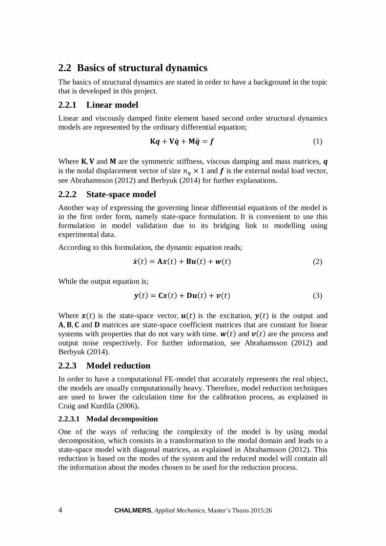
2.3.1 Modelling of spot welds
Spot welds in between two parts add significant stiffness to the welded area in real
components, as it constrains their relative movement. This kind of connection is
modelled using solid elements and a connection called rbe3 element in the finite
element software, as shown in Figure 1.
Upper part removed
Figure 1: Modelling of spot welds in the finite element software
A solid element is used between the two components that have been welded, with
approximately the same size as the area that the spot weld occupies in reality. The
rbe3 elements are then used to connect the edges of the solid element with the
corresponding part. Each face of the solid element contains four vertices and each of
these vertices is connected to the four nodes of the closest shell element, as it is
possible to see in the lower part of Figure 1.
Welded parts
(shell elements)
rbe3 elements
Solid element

6 CHALMERS, Applied Mechanics, Master’s Thesis 2015:26
2.3.2 Modelling of adhesive
Adhesive is used in physical components to attach different parts to each other. The
adhesive also adds stiffness into the system, as the degrees of freedom of the attached
areas are significantly prevented from moving, even if the degree of constraint is
considerably lower than when using spot welds. Figure 2 shows the way of modelling
the adhesive.
Figure 2: Modelling of adhesive in the finite element software
As it is possible to observe, the adhesive is modelled in the finite element software
employing solid elements forming a string. These solid elements, as in the case of
modelling welding, are connected to the attached parts using rbe3 elements. The
vertices at each face of the solid elements are connected to the closest nodes of the
shell elements.
2.3.3 Modelling of screws
Using screws is another way of connecting different parts of a component through
thread holes. The screw connects the areas of the parts around the hole constraining
their degrees of freedom. The way to model this numerically consists in using beam
elements, named cbar, in between two points of the grid; see BETA CAE Systems
S.A. (2014) for further explanations. The cbar element connecting the parts is shown
in Figure 3.
Attached parts
using adhesive
(shell elements)
Upper part removed
Solid elements
representing
adhesive string
rbe3 elements

CHALMERS, Applied Mechanics, Master’s Thesis 2015:26 7
Screwed parts
(shell elements)
Figure 3: Modelling of screws in the finite element software
The ends of the beam element are then connected with the holes of the two parts being
attached using rbe2 rigid elements.
2.3.4 Rbe2 and rbe3 connections
These connections are used to define a rigid body element between grid points in the
FE-model. In the case of the rbe2 connection, this element is a rigid body with
independent degrees of freedom specified at a single grid point, named the master
point, and with dependent degrees of freedom at an arbitrary number of grid points,
called slaves, surrounding the master grid point. It is employed to model the screws
and it can be seen in Figure 3.
On the other hand, the rbe3 connection defines an interpolation constraint element
between grid points. The element defines the motion at a reference grid point as the
weighted average of the motions at a set of other points. This is used to model the
adhesive and the spot welds, shown in Figure 1 and Figure 2. Further explanations can
be found in the BETA CAE Systems S.A. (2014) manual.
The rbe2 element creates a stiffer connection compared to the rbe3 element, since all
the slave points have the same motion as the master point, while in the case of the
rbe3 connection the motion of the reference grid point is defined by all the other
points that it is connected to.
2.4 Pre-test planning
Experiments are required in order to conduct the calibration and validation process of
a model. A thorough planning of the testing ensures high quality test data, which
facilitates and increases the possibilities of success of this process.
2.4.1 Method of effective independence
The method of Effective Independence (EFI) is used for modal test planning, as
explained in Abrahamsson (2012). According to this method, a set of candidate nodes
for the optimal sensor locations is defined. When defining these nodes, physical
feasibility to place the accelerometers at these positions has to be taken into account;
i.e. the nodes have to be at locations where it is possible to attach accelerometers at
the tailgate, so the surface has to be accessible and flat.
rbe2 elements Upper part removed
cbar element

8 CHALMERS, Applied Mechanics, Master’s Thesis 2015:26
This method will then select the most optimal sensor locations to observe the
dynamics of the system for the desired number of eigenmodes, based on the
eigenvectors of the modes obtained from the FE-model. The method calculates the
contribution of the candidate sensor locations to the Fisher information matrix and
iteratively removes the candidates which make the least contribution to this matrix,
keeping the determinant of the Fisher information matrix as large as possible, see
Kammer, D. (1991). Therefore, the number of candidates is reduced to the desired or
available number of accelerometers.
2.4.1.1 Fisher information matrix
The Fisher information matrix measures the amount of information that an observable
variable carries. It is the inverse of the variable covariance matrix, and its determinant
is used to scale the contribution of the candidates regarding the dynamics of the
system, as stated in Abrahamsson (2012). Then, removing one candidate at a time, the
determinant of the Fisher information matrix is calculated; the removed candidate that
results in the highest determinant is providing the least information about the system,
so that is the one to disregard. Further explanations are provided in Kammer and
Tinker (2004).
The Fisher information matrix becomes singular when the number of candidate
sensors is less than the number of aimed modes to be observed. Therefore, the
minimum number of sensors to be used cannot be lower than the number of target
eigenmodes.
2.4.2 Observability and controllability
State observability and state controllability are important conditions to be considered
in vibration testing. State observability tells whether the states of the system are
observable and it is used to determine if the target eigenmodes can be captured with
the chosen sensor locations. On the other hand, state controllability clarifies whether
those target eigenmodes are excited with the chosen actuator locations and therefore
can be measured in the testing, as explained in Abrahamsson (2012).
2.4.2.1 Gramians
The controllability and observability gramians are used to evaluate whether a system
is controllable/observable for a certain time interval. This is fulfilled if the gramian
matrix is non-singular and therefore invertible; see Abrahamsson (2012) and Berbyuk
(2014).
2.4.2.2 Balanced realization
The mentioned gramians are control time dependant and consequently not unique.
Besides, as they are not invariant to similarity transformation, if such a transformation
of the state-space system is performed and an equivalent realization is calculated,
different gramians are obtained.
As a result, a similarity transformation that leads to a balanced realization has to be
accomplished. This realization makes the observability and controllability gramians to
become diagonal and equal and thus they are balanced for all control and observation
ranges, see Moore (1981) for further explanations.
CHALMERS, Applied Mechanics, Master’s Thesis 2015:26 9
2.5 Testing
In order to obtain as accurate as possible test data required to calibrate the FE-model,
the vibration testing to collect this data has to be carefully performed, thus the data is
an exact representation of the real test objects.
Therefore, specific hardware and excitation method are used in vibration testing to
guarantee the success of the measurements. Besides, special care has to be taken with
the set-up of the experiment in order for non-desirable factors not to affect the results
of the measurements.
2.5.1 Vibration testing hardware
The hardware used for vibration testing consists of different parts, as explained in
Abrahamsson (2012). The main component that the tests are based on is the
transducer, which converts a signal in one form of energy into another energy form.
The data acquisition of the measurements is achieved using sensors, a type of
transducer whose aim is to sense or detect some characteristics of its environment and
convert these events generally into electric signals.
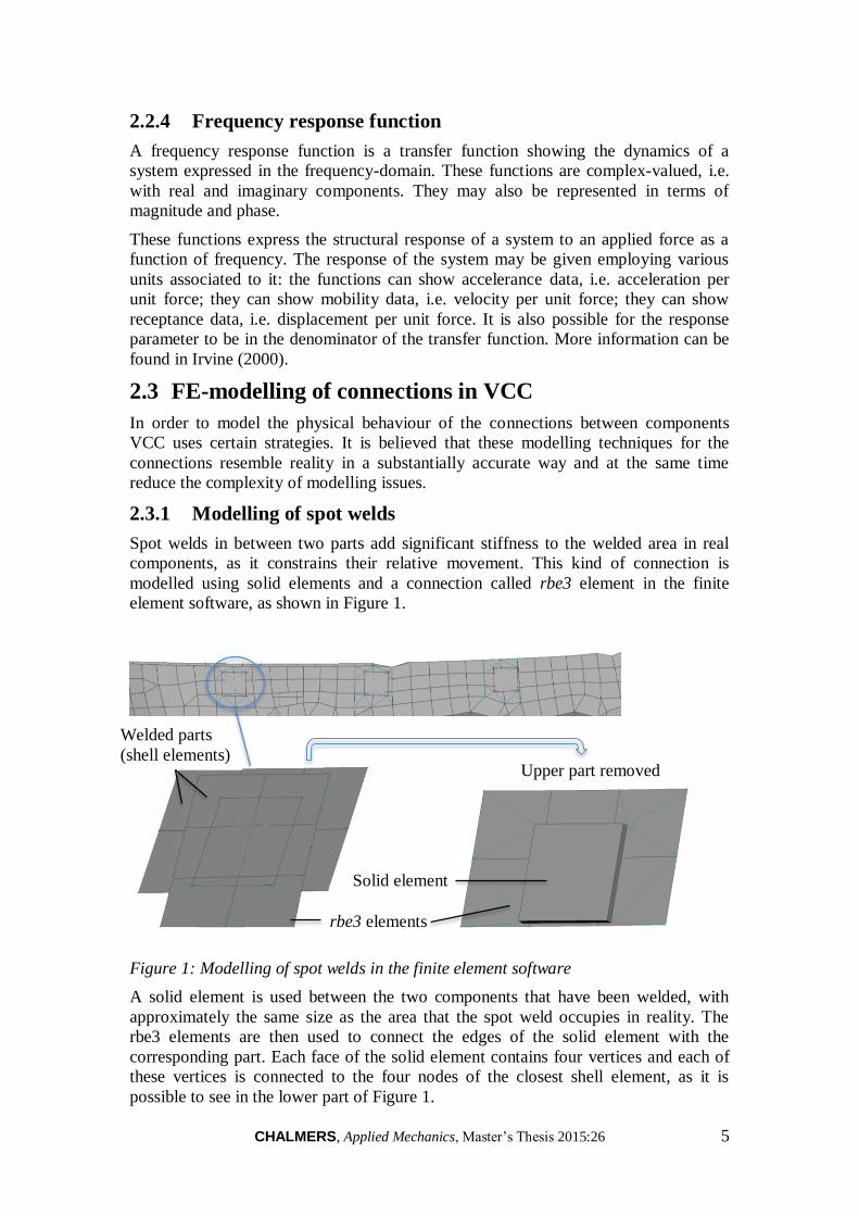
The electric signals that the sensors produce are transferred into the Data Acquisition
(DAQ) system. DAQ is responsible for sampling this signal to get the data of the
sensor on a digital form in order for the computer to process this data. A schematic
arrangement of the hardware required for vibration testing can be seen in Figure 4.
Figure 4: Instruments required for vibration testing. Retrieved from Abrahamsson
(2012).
As it is possible to observe, the signals are sent to and received from the DAQ system,
which is connected to the computer. The testing parameters are usually defined by the
engineer in the testing software. Hence, the profile of the system excitation is
transferred to the DAQ, which converts the digital current into analogue current. This
signal is then amplified using a power amplifier and transferred into an
electromagnetic shaker, which converts the electric current into force excitation. This
actuator drives a rod called stinger that is attached to the test article and therefore the
excitation is only transmitted in the longitudinal direction without loading the test
article in its transversal direction.
As a result, the test article starts vibrating under the conditions defined by the
engineer. This vibration is measured by sensors to obtain the dynamics of the object:
the response sensing is usually captured in terms of acceleration by the use of
accelerometers. On the other hand, a reference is required to calculate the aimed FRFs

10 CHALMERS, Applied Mechanics, Master’s Thesis 2015:26
of the system: the input loading into the system. This load is measured by the use of
force transducers.
These sensors convert the sensed acceleration and the force applied into the system
into an electric signal that is sent to the DAQ. After converting these signals from
analogue to digital current and processing them in the DAQ system, the processed
data is transformed from time domain to frequency domain data and the FRFs of the
locations where the accelerations were measured are calculated and showed in the
testing software.
2.5.1.1 Accelerometers
An accelerometer is a type of sensor that senses the acceleration motion and converts
this energy into an electric signal. Accelerometers are usually based on the
piezoelectric phenomenon: piezoelectric materials induce an electric charge when
strain is applied into them, and vice versa. Therefore, piezoelectric accelerometers
contain an inertial mass that presses a piezoelectric crystal when it senses
acceleration. Consequently, the crystal experiences a force which leads to a
proportional strain, inducing an electric charge.
Special care has to be taken when mounting the accelerometers onto the object to be
tested. It could happen that the surface where the accelerometer is attached does not
experience exactly the same motion as the accelerometer’s reacting piezoelectric
material, mainly at high frequencies. Hence, the surface where the accelerometer is
mounted has to be smooth and flat in order to avoid any dissimilarities. A thin layer of
silicone grease is used to ensure identical motion in the surface and in the attached
accelerometer.
Moreover, the fundamental eigenfrequency of the accelerometer has to be taken into
account. Results measured by the accelerometer in a frequency range approaching or
exceeding this frequency should not be considered.
Apart from that, each accelerometer has to be calibrated before and after the test are
performed in order to ensure that non optimal test data is processed. This calibration
is conducted using a calibrator; see Abrahamsson (2012) for further explanations.
2.5.1.2 Force transducers
A force transducer is a sensor that induces an electric charge when it is stressed by a
load. This sensor is also based on the piezoelectric effect, so when the force is applied
to it and therefore the piezoelectric crystal experiences a change in the strain, the
crystal generates an electrostatic charge proportional to the input force. The generated
electric signal is then collected on the electrodes between the crystals.
Ideally, the force transducers should only be subjected to uniaxial loading in the
aimed direction. However, loads in other directions are also applied in reality; special
care should be taken to lower these loads as much as possible so only load in the
desired axis is transmitted to the sensor. Hence, the stinger transmitting the load from
the shaker to the structure has to be as perpendicular as possible with respect to the
surface where the force transducer is attached.
The measured force in the transducer can slightly vary from the force applied by the
actuator and also from the load transmitted to the test article. This is caused due to
inertia loading induced by acceleration of the mass distributed over the sensor. In
CHALMERS, Applied Mechanics, Master’s Thesis 2015:26 11
order to minimise the variation between the load transmitted from the shaker to the
test object and captured by the force transducer, a proper mounting of the force
transducer to the article is necessary. If the sensor is correctly attached onto a flat
surface of the structure, this inertia is minimised. Moreover, if the contact surfaces
between the force transducer and the test object are totally parallel, bending moment
and edge loading will be reduced. Using a thin layer of lubricant between the contact
surfaces will also improve the quality of the measurements and avoid short duration
overloads due to the direct impact between metals, as mentioned in Abrahamsson
(2012).
2.5.2 Set-up of the experiments
The purpose of the measurements is to obtain the FRFs containing the information
about the flexible modes of the test object to be compared with the information
extracted from the FE-model. Hence, the testing has to be conducted in free support
conditions, mimicking that it is freely suspended in space, as mentioned in
Abrahamsson (2012). The structure is then hanged in such a way that the free
condition is obtained and no unnecessary constraints are added into the system.
Particular attention has to be paid to the rigid body modes of the structure; as the
article is supported by some means, the rigid body modes are no longer of 0 Hz, and
the support can therefore affect the flexible modes.
The best way to approach this situation is by providing a suspension system: the test
article is supported on very flexible spring-like elements which could be light elastic
bands, called bungee cords. Consequently, the six rigid body modes that the structure
possesses will be very low in relation to the flexible modes. The rigid body modes are
assumed not to have influence on the flexible modes when the highest rigid body
mode frequency is less than 10 − 20% of the first natural mode frequency, according
to Abrahamsson (2012).
These bungee cords should ideally be placed as close as possible to nodal points of
the first flexible modes and normal to the main direction of vibration in order not to
encounter problems with resonances of the bungee cords affecting the dynamics of the
test object. It is also important to note that the suspension system can add significant
damping to lightly damped test articles, affecting the response of the system.
When mounting the accelerometers into the test article, the possibility of adding
damping into the system has to be avoided. Hence, accelerometers have to be properly
attached into the system and having cables in contact with the object has to be
avoided to the extent possible. If necessary, these cables have to be fixed into the
system, using tape for instance, to prevent relative motion between the cable and the
object.
As regards to the input excitation, the actuator is connected to the stinger, which is in
turn connected to the force transducer that is attached onto the surface of the test
article. The force is transmitted through these components exciting the structure;
hence, these connections have to be properly mounted to ensure the correct
transmission of the excitation. The stinger has to be long enough to ensure only
uniaxial load in the direction of the rod is transmitted from the shaker; however, no
low-frequency resonances should be present locally in the stinger to prevent the
transmission of them into the structure. As a result, the stinger has to be totally normal
to the force transducer, and in turn the contact surface between the sensor and the test
object has to be completely parallel.
12 CHALMERS, Applied Mechanics, Master’s Thesis 2015:26
2.5.3 System excitation
Due to the accuracy in the results and the suitability of the method, periodic excitation
is usually used for model calibration rather than aperiodic excitation. This type of
excitation is characterised for being repeated every time interval, called the cycle.
Periodic excitation is more suitable for this purpose because it leads to a steady-state
condition after the vibration is applied during a number of cycles, when the system
becomes asymptotically stationary: the initial transient diminishes and the response
becomes steady-state with very good period-to-period repeatability. This is fulfilled
when the test object is damped, a requirement that all practical structures conform,
and when the system is linear.
There are a number of periodic excitation types; the classical method for vibration is
the mono-frequency or stepped-sine testing, which excites the system with one
frequency at a time. However, new excitation types have been developed, which use a
more complex periodic input signal that contains all the frequencies in the range of
interest at the same time. Such examples are random or chirp signals, as further
explained in Abrahamsson (2012).
2.5.3.1 Stepped-sine excitation
This type of testing sends a discrete sinusoid signal to the actuator with fixed
amplitude and frequency; see Ewins (2000) for further explanations. In order to cover
the frequency range of interest, the source signal frequency is stepped from one
discrete frequency to the next according to the established resolution.
Nevertheless, before measuring the response and moving to the next frequency step, it
is necessary to ensure that the steady-state conditions are achieved. This is conducted
by delaying the start of the measurement when stepping into a new frequency. The
number of cycles before the transient response is diminished depends on various facts:
how close the excitation frequency is from an eigenfrequency or an anti-resonance of
the system, the damping lightness of a mode close in frequency and the abruptness of
the signal when moving to a new frequency step. These characteristics cause the
transient effect to last longer and therefore the delay before the response is measured
has to be greater.
The test data acquired with stepped-sine vibration is more precise due to the accuracy
of signal and noise control compared to other periodic excitations, which employ
different signal processing. This signal provides the opportunity of monitoring the
harmonic distortion and the signal-to-noise ratio, ensuring for instance that non-linear
responses are avoided in the system. On the other hand, the main disadvantage of the
stepped-sine testing strategy consists in the long testing time.
2.5.3.2 Burst-random excitation
All the frequencies in the range of interest are sent to the actuator in the input signal
simultaneously when using burst-random excitation. This is achieved by using
superposition of several sinusoids at the same time and extracting the response of
each component with discrete Fourier transformation, as explained in Ewins (2000).
Random excitation can be of two types: full cycle excitation, when excitation signal
energy is sent during the whole cycle, or burst excitation, when the signal source is
silent at the end of the period. The advantage using burst-random excitation signal is

CHALMERS, Applied Mechanics, Master’s Thesis 2015:26 13
that when signal energy is sent the response shows a transient behaviour while the
response diminishes during the silent interval. Therefore, it is ensured that at the
beginning of the next cycle little influence from the previous one is measured.
A number of cycles are measured when this strategy is used and the average is taken
in order to remove the possible signal noise and ensure accuracy of the test data. The
advantage when using this method consists in the rapidness of the measurement time;
nevertheless, it does not provide the opportunity to monitor the distortion to evaluate
whether the system behaves linearly or not.
2.5.4 Signal processing
Signal processing in vibration testing is usually performed using discrete Fourier
transformation. It is based on the spectra of the test stimuli and the response of the
system under this excitation. The DAQ system is the instrument responsible for
performing the spectral analysis, by discretising the time signals sampled over the
period, as explained in Ewins (2000).
However, several features can arise in the process of digital Fourier analysis which
might lead to erroneous results; the discretisation approximation and the necessity to
limit the length of time history can cause the test data to be altered. Signal aliasing
and frequency leakage are the most relevant features that can emerge while doing
measurements. Consequently, a number of measures exist in order to prevent these
problems from happening, such as windowing, filtering, zooming or averaging, which
are processed by the DAQ system. Detailed explanations of the features that can arise
and how to take care of them can be found in Ewins (2000).
2.6 System identification
In order for test data to be used for calibration and validation process, a state-space
model of the measured data has to be estimated. System identification is used to
calculate the state-space system matrices, which are previously mentioned in Section
2.2.2. System identification is a non-iterative convergent process that relies heavily on
numerical linear algebra, but the theory behind is not going to be treated in this thesis.
To understand the theory, the reader is referred to Ljung (1987).
The N4SID algorithm was developed by Van Overschee and De Moor (1994) and
(1996) to identify mixed deterministic-stochastic systems by determining state
sequences through the projection of input and output data. Even if it was intended for
time domain test data, the algorithm was adjusted to work for discrete frequency data
by McKelvey et al. (1996). A short description of the N4SID algorithm together with
its restrictions is provided in Abrahamsson (2012).
This method gives the possibility to use non-uniform frequency data, providing the
user more flexibility. Besides, the main advantage of this method consists in only
requiring the model order estimation of the significant states of the measured
frequency range, i.e. the appropriate model order, to calculate the corresponding state-
space model.
2.7 Correlation indicators
There are several available methods to compare the correlation between the FE-model
and the measured data. The most straightforward way of comparing how well the
results from simulations match with the physical articles is by contrasting the
resonance frequencies from test data with the eigenvalues extracted from the FE-

14 CHALMERS, Applied Mechanics, Master’s Thesis 2015:26
model. A more advanced strategy consists in evaluating the eigenmodes of both
systems and thus comparing their geometrical shape at the flexible modes. Another
way of comparing them consists in calculating the deviation metrics of both systems’
frequency response function.
2.7.1 Modal Assurance Criterion
The Modal Assurance Criterion (MAC) is used to compare the co-linearity of the
eigenvectors measured in the experiments with the eigenvectors extracted from the
FE-model. Since the test is conducted only at a certain amount of locations of the test
object, the corresponding eigenvectors for these positions are calculated from the
simulations. Detailed explanations on how to perform the MAC correlation and
important features about it can be found in Allemang (2003).
Practically, when computing the MAC correlation the angle between the eigenvectors
is being calculated; see equation (5.11) in Abrahamsson (2012). Therefore, if the
modes have approximately the same angle, meaning that the MAC number is unity or
close to it, these modes are highly correlated. Otherwise, if the modes are orthogonal,
the MAC number approaches zero.
If the FE-model and the test article are very similar, then the MAC matrix should
ideally contain ones along its diagonal. This occurs as long as no modes are missing
in both systems and assuming the eigenmodes have been ordered in increasing
frequency order. However, this is not usually the case: even for FE-models that
closely resemble reality, it is often the case that two eigenmodes are close in
frequency and the corresponding eigenvectors change significantly for small
perturbations in model parameters.
In case two modes are shifted in eigenfrequencies, a simple re-arrangement of the
modes in either the test data or the FE-model data would give a MAC matrix with
diagonal elements much closer to the unity.
2.7.1.1 Coordinate Modal Assurance Criterion
A modified version of the MAC indicator is the CO-ordinate Modal Assurance
Criterion (COMAC). This method allows checking whether any of the measured
channels lead to erroneous data by considering individually a channel from the
measurements with its corresponding degree of freedom in the FE-model; see
Allemang (2003) for further explanations.
This strategy calculates a COMAC number for each sensor used in the measurements
that can vary between zero and one; see equation (5.12) in Abrahamsson (2012). If a
set of eigenvectors give good correlation according to MAC and any of the locations
used for this calculation gives a COMAC number far from zero, this is an indication
that an error occurred most likely with this channel in the experiments (or with this
degree of freedom in the FE-model). An experimental error could mean loose
accelerometers during measurements, sensor wires incorrectly mounted or erroneous
sensor calibration.
2.7.2 Deviation metric
A simple and optimal way of calculating whether the FE-model approaches the
physical object is achieved using deviation metrics. The question arises whether to
compute this metric using time domain, frequency domain or modal domain data.
CHALMERS, Applied Mechanics, Master’s Thesis 2015:26 15
Computing the deviation metric using time domain data is not feasible due to the high
amount of data which will require heavy computational cost and the presence of noise
in the test data which will blur the metric.
On the other hand, even if the modal domain deviation metric would in advance look
promising due to the compact description of the dynamics of the system, some
problems can be encountered when using it. In order to relate FE data with
experimental data, the modes have to be correctly paired: it is not sufficient with
ordering the eigenfrequencies in ascending order, as the mode shapes can be shifted in
frequency in the FE-model compared to the test data. The modes are required to be
paired using MAC correlation analysis. Besides, it is probable that all the modes are
not accurately captured in the measurements due to some modes not being
controllable from the shaker position or not being observable at any sensor location.
Consequently, frequency domain based metric seems to be the optimal strategy to
calculate the deviation metric between analytical and experimental results, as
mentioned in Abrahamsson (2012).
2.7.2.1 Frequency domain deviation metric
The deviation metric 𝑄 in frequency domain is calculated based on the frequency
response functions. Therefore, the amplitudes of vibration at all frequencies included
in the frequency range of interest are captured in the deviation, including the
resonances and anti-resonances. In order not to discriminate the deviation at
frequencies where the structural response is small, the deviation is calculated in
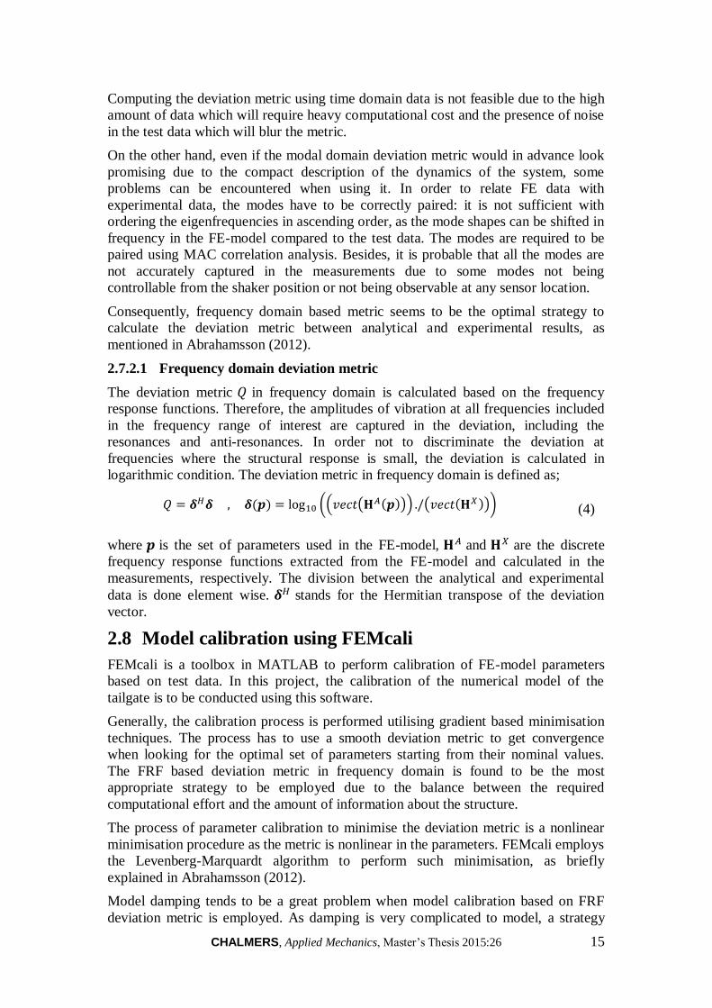
logarithmic condition. The deviation metric in frequency domain is defined as;
𝑄 = 𝜹𝐻𝜹 , 𝜹(𝒑) = log10 ((𝑣𝑒𝑐𝑡(𝐇𝐴(𝒑))) ./(𝑣𝑒𝑐𝑡(𝐇𝑋))) (4)
where 𝒑 is the set of parameters used in the FE-model, 𝐇𝐴 and 𝐇𝑋 are the discrete
frequency response functions extracted from the FE-model and calculated in the
measurements, respectively. The division between the analytical and experimental
data is done element wise. 𝜹𝐻 stands for the Hermitian transpose of the deviation
vector.
2.8 Model calibration using FEMcali
FEMcali is a toolbox in MATLAB to perform calibration of FE-model parameters
based on test data. In this project, the calibration of the numerical model of the
tailgate is to be conducted using this software.
Generally, the calibration process is performed utilising gradient based minimisation
techniques. The process has to use a smooth deviation metric to get convergence
when looking for the optimal set of parameters starting from their nominal values.
The FRF based deviation metric in frequency domain is found to be the most
appropriate strategy to be employed due to the balance between the required
computational effort and the amount of information about the structure.
The process of parameter calibration to minimise the deviation metric is a nonlinear
minimisation procedure as the metric is nonlinear in the parameters. FEMcali employs
the Levenberg-Marquardt algorithm to perform such minimisation, as briefly
explained in Abrahamsson (2012).
Model damping tends to be a great problem when model calibration based on FRF
deviation metric is employed. As damping is very complicated to model, a strategy
16 CHALMERS, Applied Mechanics, Master’s Thesis 2015:26
consisting in assigning a simple representation for modelling convenience is usually
employed. This representation for the energy dissipation effects in the structure is
generally accurate enough for the calibration process. Such strategy is modal
damping, when the damping found in the experiments is applied to the FE-model.
However, mapping the experimental modes to the numerical model is a difficult task.
As a result, the damping equalization method is employed instead in the FEMcali
toolbox as explained in Abrahamsson and Kammer (2015), which consists in using
the same amount of damping for all the modes, avoiding any problems with mode
paring. According to this method, a value of modal damping is imposed to both the
FE-model and the mathematical model obtained from the experimental data. Hence,
the damping level of the system identified from raw measurements can be modified
maintaining the stiffness and inertia properties intact. It is then possible to conduct
model calibration of the numerical model towards this fictitious experimental model
to calibrate the parameters that are in relation with the mass and stiffness properties of
the structure.
Model calibration has to be based on really fast computations to obtain the FRFs of
the system with each new parameter setting in the iterative process to look for the
minimum deviation metric. In order for this procedure to be conducted in a practically
useful time period, model reduction of the FE-model is required: the reduced model is
then used as a surrogate model. The eigenmodes of the structure at its nominal
parameter setting is employed for the reduction, including all the modes in a
frequency range that significantly overlaps the frequency range of interest. The same
surrogate model is utilised during the whole calibration cycle without recalculating it
as the parameter setting is modified iteratively.
The gradients of the structural matrices are calculated based on finite difference
approximation scheme in the FE-model, i.e. the response of the system under a tiny
difference in one of the parameters to be calibrated in the model is calculated at a time
and therefore the gradient is computed employing this and the nominal response.
The first order expansion of the Taylor series of the reduced order model is used as
the surrogate model, thus it is linear in the parameters. This surrogate model has been
found to be an accurate representation of the complete FE-model for the interested
frequency range, as mentioned in Abrahamsson (2012). As a result, the reduced order
model and its gradients are established from the full size FE-model at the beginning of
the calibration procedure, and no further evaluation of the FE-model is required;
hence, the computational effort is generally low.
2.8.1 FEMcali working procedure
The input FEMcali requires consists in the frequency response functions obtained
from measurements and the corresponding identified state-space model as regards to
test data to calibrate against. On the other hand, regarding the analytical data, it
requires the input file defining the FE-model and connecting the FE software apart
from the degree of freedom number corresponding to the accelerometer location and
direction.
At the beginning of the calibration process, the mass and stiffness matrices are
extracted from the FE-model and the surrogate model is established by estimating the
modal damping matrix according to the damping equalization method mentioned

CHALMERS, Applied Mechanics, Master’s Thesis 2015:26 17
above. The gradients of the structural matrices corresponding to the parameters to be
calibrated are also calculated by adding a small variation of each of these parameters
into the FE-model and extracting the mentioned structural matrices showing the
response of the system to the infinitesimal parameter variations; the gradient to each
parameter variation is then computed utilising this and the nominal matrices.
The state-space model representing raw test data is then adjusted according to
damping equalization.
At this point, the calibration procedure starts on the surrogate model comparing it
with the modified state-space model. This process is conducted employing the
Lavenberg-Marquardt minimiser searching for the minimum deviation metric.
Randomised starts are utilised to achieve the calibration solution resulting in the
minimum deviation metric when comparing the numerical model to the identified
model out of the experimental data. For further explanations, the reader is referred to
Abrahamsson and Kammer (2015).
Finally, FEMcali reports the calibrated parameters together with the results of the
calibration optimisation.
18 CHALMERS, Applied Mechanics, Master’s Thesis 2015:26
3 FE-model of the tailgate
An FE-model of the V40 vehicle tailgate to be calibrated and validated was provided
by VCC for this thesis in the pre-processor ANSA, which belongs to BETA CAE
Systems S.A. This model was assumed to be verified (see Section 2.1.1), thus the
outputs from the model are supposed to be in substantially great accordance with the
underlying partial differential equation it is supposed to mimic. The real tailgate can
be seen in the figure in the cover.
As the process of calibration and validation was defined to be conducted only on the
metal parts, the trim components and the glass were removed from the FE-model.
Furthermore, the model was dependent on the objects to be tested. These were
ordered from the production line and it was uncertain at which stage of the production
they were retrieved from. Once the test articles were available, it was possible to
check which parts the tailgate was composed of. Therefore, the FE-model was
adapted so only the components of the physical tailgate to be tested were included in
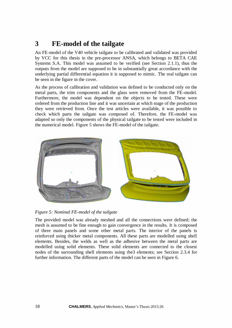
the numerical model. Figure 5 shows the FE-model of the tailgate.
Figure 5: Nominal FE-model of the tailgate
The provided model was already meshed and all the connections were defined; the
mesh is assumed to be fine enough to gain convergence in the results. It is composed
of three main panels and some other metal parts. The interior of the panels is
reinforced using thicker metal components. All these parts are modelled using shell
elements. Besides, the welds as well as the adhesive between the metal parts are
modelled using solid elements. These solid elements are connected to the closest
nodes of the surrounding shell elements using rbe3 elements; see Section 2.3.4 for
further information. The different parts of the model can be seen in Figure 6.

CHALMERS, Applied Mechanics, Master’s Thesis 2015:26 19
Figure 6: Parts composing tailgate in the FE-model
All the reinforcements and the wiper component are attached to the main panels using
spot welds. The metal panels are also attached to each other using spot welds in the
inner areas, while in the outer areas these panels are connected using the seaming
technique.
This technique consists in a metalworking process where the edge of a metal sheet is
rolled flush to itself, containing the edge of the other metal panel in the middle; see
Benson (1997) for further explanations. The edge of the outer panel then ends up with
a U-shape, containing the edge of the inner metal sheet inserted in the U-shape.
Seaming is used in the outer area of the tailgate to reinforce the edge and improve the
appearance, apart from hiding possible burrs and rough edges.
In reality, the seaming contains a sealing adhesive in between the two metal sheets
that are connected all over the U-shaped edge. This adhesive, which is rather soft, is
used to avoid any external dirt penetrating the connection, so it acts as a sealing.
On the other hand, due to the complexity of modelling the adhesive all over the U-
shaped edge, the adhesive is only added on one side of the U-shape in a rather simple
way in the analytical model in order to make the connection between the two metal
sheets, so the physical behaviour is mimicked and the real dynamics of the system are
captured.
Figure 7 shows an extract of the FE-model containing the modelling of the seaming.
Outer lower part
Inner part Outer upper part
Upper reinforcements
Wiper motor bracket
Lower reinforcements
Latch reinforcement
Upper adhesive
Spot welds
Lower adhesive

20 CHALMERS, Applied Mechanics, Master’s Thesis 2015:26
Figure 7: Modelling of the seaming in the FE-model
In this way, a constraint on the inner and outer metal sheets is imposed, so the
stiffness of the sealing in the real component is transferred to the FE-model.
Apart from the parts shown in Figure 6, the FE-model contains some screws
connecting the metal panels, using beam elements and rbe2 elements to connect the
beam to the panels, as previously mentioned in Section 2.3.3.
3.1 Parameters in the FE-model
Each part in the FE-model is given a property, and each property in turn is given a
material. Looking at the parts shown in Figure 6, the parameters that define the FE-
model are stated in Table 1.
Table 1: Parameters defining the FE-model
Name Element
type
Stiffness
𝐸 [GPa] Poisson’s
ratio 𝜈 [−] Density
𝜌 [kg
m3]
Thickness
𝑡 [mm]
Inner part Shell 210 0.3 7850 0.7
Outer upper
part Shell 210 0.3 7850 0.7
Outer lower
part Shell 210 0.3 7850 0.8
Upper
reinforcements Shell 210 0.3 7850 1.2
Lower
reinforcements Shell 210 0.3 7850 2
Latch
reinforcement Shell 210 0.3 7850 1.5
Wiper motor
bracket Shell 210 0.3 7850 1.5
Adhesive Solid 0.006 0.4 1000 −
Spot welds Solid 210 0.3 − −
Screws Bar (rod) 210 0.3 7850 −
Apart from these parameters, the FE-model is defined by the geometry of each
component and the rbe2 and rbe3 elements connecting the different parts.
Outer metal sheet (shell elements)
Inner metal sheet (shell elements)
Adhesive (solid elements)
Rbe3 elements

CHALMERS, Applied Mechanics, Master’s Thesis 2015:26 21
4 Testing process
Test data is required in order to perform the process of calibration and validation. The
calibration and validation is conducted in the FE-model with the nominal model
parameters, which are required to be calibrated. Therefore, a pre-test planning is
accomplished based on the nominal FE-model of the tailgate explained in Chapter 3
in order to ensure a successful test outcome, assuming that the model matches reality
at a certain grade of accuracy with its nominal parameter values.
4.1 Pre-test planning
It is assumed that an adequate FE-model of the test object is at hand which resembles
acceptably the physics of the real tailgate and that the dynamic characteristics of the
model are suitable for the planning of sensor layout.
The aim of this planning consists in looking for the optimal sensor and actuator
positions in the test, such that as much information about the dynamics of the system
as possible is obtained during the experiments.
Before starting to choose the mentioned positions, an evaluation of testing hardware
usability is conducted. According to VCC, most of the equipment is accessible at all
times, but there is significant risk for accelerometers not being constantly available. It
is decided to use uniaxial accelerometers for the testing due to less usage of these.
Besides, it is assumed that approximately 30 accelerometers are possible to be used
during the measurements.
VCC is interested in calibrating the model in the frequency range in which the vehicle
vibrates according to road noise; i.e. the frequency range approximately in between
0 − 300 Hz. Consequently, an investigation of the flexible modes of the system at this
frequency range is conducted. The nominal FE-model is exported from the pre-
processor Ansa and an eigenmode analysis of the system is accomplished using the
solver MSC Nastran. The analysis of the modes is performed using the post-processor
µETA. This frequency range contains 31 natural frequencies apart from the rigid body
modes and the dynamics of these modes are investigated.
A set of candidate nodes that are potential sensor locations in the test are chosen in the
FE-model. A couple of hundreds of candidates are chosen, covering all the surfaces of
the FE-model and mainly placing the points at the locations where the dynamics of
the system are more pronounced according to the mentioned analysis. This process is
conducted taking into account the reachability and flatness of the surfaces where the
nodes are located, thus it is feasible to attach an accelerometer physically at those
locations. A local coordinate system is created at each of these candidate nodes with
the z-direction normal to the surface; the uniaxial accelerometers sense in the normal
direction to the attached surface, then the response from the FE-model is desired to be
obtained in this direction as well.
Out of the selected candidate nodes, the actual sensor locations are calculated using
the EFI method, see Section 2.4.1. This process is conducted in MATLAB with an
available script that accomplishes the method. The method requires the eigenmodes of
the candidate nodes: an analysis of the FE-model is conducted using the solver to
obtain the z-displacement of the set of candidates at their eigenfrequencies, which
corresponds to the eigenvectors of the modes of the system for these locations.
22 CHALMERS, Applied Mechanics, Master’s Thesis 2015:26
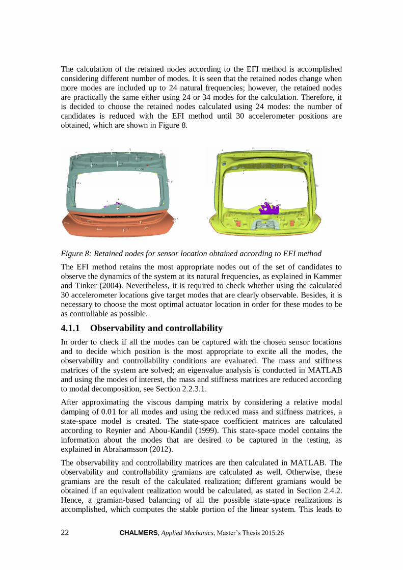
The calculation of the retained nodes according to the EFI method is accomplished
considering different number of modes. It is seen that the retained nodes change when
more modes are included up to 24 natural frequencies; however, the retained nodes
are practically the same either using 24 or 34 modes for the calculation. Therefore, it
is decided to choose the retained nodes calculated using 24 modes: the number of
candidates is reduced with the EFI method until 30 accelerometer positions are
obtained, which are shown in Figure 8.
Figure 8: Retained nodes for sensor location obtained according to EFI method
The EFI method retains the most appropriate nodes out of the set of candidates to
observe the dynamics of the system at its natural frequencies, as explained in Kammer
and Tinker (2004). Nevertheless, it is required to check whether using the calculated
30 accelerometer locations give target modes that are clearly observable. Besides, it is
necessary to choose the most optimal actuator location in order for these modes to be
as controllable as possible.
4.1.1 Observability and controllability
In order to check if all the modes can be captured with the chosen sensor locations
and to decide which position is the most appropriate to excite all the modes, the
observability and controllability conditions are evaluated. The mass and stiffness
matrices of the system are solved; an eigenvalue analysis is conducted in MATLAB
and using the modes of interest, the mass and stiffness matrices are reduced according
to modal decomposition, see Section 2.2.3.1.
After approximating the viscous damping matrix by considering a relative modal
damping of 0.01 for all modes and using the reduced mass and stiffness matrices, a
state-space model is created. The state-space coefficient matrices are calculated
according to Reynier and Abou-Kandil (1999). This state-space model contains the
information about the modes that are desired to be captured in the testing, as
explained in Abrahamsson (2012).
The observability and controllability matrices are then calculated in MATLAB. The
observability and controllability gramians are calculated as well. Otherwise, these
gramians are the result of the calculated realization; different gramians would be
obtained if an equivalent realization would be calculated, as stated in Section 2.4.2.
Hence, a gramian-based balancing of all the possible state-space realizations is
accomplished, which computes the stable portion of the linear system. This leads to
CHALMERS, Applied Mechanics, Master’s Thesis 2015:26 23
an equivalent realization for which the controllability and observability gramians are
equal and diagonal, considering that the system is stable.
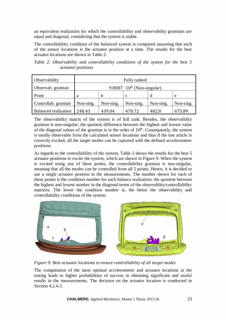
The controllability condition of the balanced system is computed assuming that each
of the sensor locations is the actuator position at a time. The results for the best
actuator locations are shown in Table 2.
Table 2: Observability and controllability conditions of the system for the best 5
actuator positions
Observability Fully ranked
Observab. gramian 9.8087 ∙ 106 (Non-singular)
Point a b c d e
Controllab. gramian Non-sing. Non-sing. Non-sing. Non-sing. Non-sing.
Balanced realization 248.43 439.04 470.72 482.8 675.89
The observability matrix of the system is of full rank. Besides, the observability
gramian is non-singular; the quotient difference between the highest and lowest value
of the diagonal values of the gramian is in the order of 106. Consequently, the system
is totally observable from the calculated sensor locations and thus if the test article is
correctly excited, all the target modes can be captured with the defined accelerometer
positions.
As regards to the controllability of the system, Table 2 shows the results for the best 5
actuator positions to excite the system, which are shown in Figure 9. When the system
is excited using any of these points, the controllability gramian is non-singular,
meaning that all the modes can be controlled from all 5 points. Hence, it is decided to
use a single actuator position in the measurements. The number shown for each of
these points is the condition number for each balance realization: the quotient between
the highest and lowest number in the diagonal terms of the observablity/controllability
matrices. The lower the condition number is, the better the observability and
controllability conditions of the system.
Figure 9: Best actuator locations to ensure controllability of all target modes
The computation of the most optimal accelerometer and actuator locations in the
testing leads to higher probabilities of success in obtaining significant and useful
results in the measurements. The decision on the actuator location is conducted in
Section 4.2.4.3.
a b
c d
e

24 CHALMERS, Applied Mechanics, Master’s Thesis 2015:26
4.2 Testing the tailgates
The measurements of the physical tailgates are performed in the modal lab in VCC.
The experiments are conducted in 3 different tailgates in order to check the dispersion
between the objects; named A, B and C.
Besides, the experiments are conducted using two different strategies: stepped-sine
excitation and burst-random excitation, as previously mentioned in Section 2.5.3.
4.2.1 Testing software
Regarding the equipment employed for the experiments, a software program
developed by Siemens PLM Software is used, called LMS Testing Solutions. This is a
complete platform for data acquisition and management applied in test-based
durability, noise and vibration engineering. Specifically, the employed software is
LMS Test.Lab REV 13A.
Two different applications of this software are used for the experiments: MIMO
Sweep & Stepped Sine Testing when the excitation is conducted with stepped-sine
signal and Spectral Testing when the type of excitation used is burst-random.
4.2.2 Testing hardware
Numerous hardware instruments are employed for vibration testing, as shown in
Figure 4. The laptop contains the software and sends the signal into the DAQ system,
i.e. the frontend. This transmits the signal into the amplifier, where the signal is
amplified and sent to the actuator. The shaker transmits the excitation into the system
through the stinger, which is attached into the force transducer; hence, the transducer
records the profile of the input excitation to the tailgate. The tailgate, which is hanged
from a test rig with the use of bungee cords, vibrates according to the excitation
signal. This vibration is sensed by the accelerometers, which transmit the response of
the system into the frontend. The frontend collects the signals received from the force
transducer and accelerometers and processes them. The processed data is collected in
the software in the laptop, allowing the engineer to evaluate the results.
4.2.2.1 Frontend and amplifier
The frontend, shown in Figure 10, is the instrument responsible for the data
acquisition.
Figure 10: Frontend used in the measurement for data acquisition. LMS SCADAS
Mobile SCR05. 40 channels, 2 outputs, 2 tachometers.

CHALMERS, Applied Mechanics, Master’s Thesis 2015:26 25
It contains 32 input channels to receive the signal from either the accelerometers or
the force transducers and 2 output channels to transmit the signal to the amplifier,
shown in Figure 11.
Figure 11: Amplifier of the excitation signal. Brüel & Kjær LDS Ling Dynamic
Systems Ltd. PAE Series PA100E - Power Amplifier.
The amplifier is the instrument responsible for receiving the low energy excitation
signal from the frontend, amplify it and transmit it to high power input to the shaker.
The amplification of the signal is adjustable by the volume control know at the right
part of Figure 11.
4.2.2.2 Actuator and stinger
The actuator is the instruments that receives the input excitation signal in electrical
current form and converts it into movement, which is applied into the tailgate. The
shaker used for the experiments is shown in Figure 12.
Figure 12: Shaker exciting the system. Brüel & Kjær LDS Ling Dynamic Systems Ltd.
Model V406 – Permanent Magnet Shaker.
The actuator has to be perfectly oriented thus the excitation signal is correctly
transmitted into the system, i.e. the excitation has to be applied normal to the surface
of the tailgate, so the height and orientation of the exciter has to be accurately
positioned. Besides, it is placed on top of a heavy structure in order to avoid
movement when exciting the system.
The excitation is transmitted into the system using the stinger, a rod composed of
plastic material shown in Figure 13.

26 CHALMERS, Applied Mechanics, Master’s Thesis 2015:26
Figure 13: Stinger transmitting the excitation into the tailgate. Stinger is attached to
force transducer.
The stinger is screwed into the actuator in one end and into the force transducer in the
other end. Plastic nuts are used to strictly tighten the stinger into these components to
make sure the stinger is not loosed from any of the parts while transmitting the
excitation.
The functionality of the stinger consists in ensuring that only excitation in the stiff
axial direction, i.e. normal to the surface of the tailgate, is transmitted into the system.
Therefore, the stinger has to be long enough to bend laterally and reduce input side
loads to the structure. In this way, the structure will be decoupled from the excitation
system avoiding dynamic effects of the shaker affecting the system. Apart from that,
the stinger also helps to isolate the exciter armature from the structure, lessening
inadvertent shocks and preventing damage to the exciter.
Nevertheless, this rod cannot be too long because this would cause resonances
possibly being created in the rod and transmitted into the system, which has to be
prevented. Besides, a long stinger might cause dynamic buckling, thus insufficient
force will be transmitted to the structure. A balance in the length of the stinger is then
required to accomplish to be as long as possible to maintain lateral flexibility but still
short enough to transmit axial force without buckling.
4.2.2.3 Sensors and calibrator
The sensors used in the tailgate testing are a force transducer to measure the input
excitation into the system and accelerometers to sense the motion of the system under
excitation, see Section 2.5.1. The employed force transducer is manufactured by to
PCB Piezoelectronics and is shown in Figure 14.
Figure 14: Force transducer to measure the input excitation. PCB Piezotronics Model
208C02 - IC𝑃® Force Sensor.
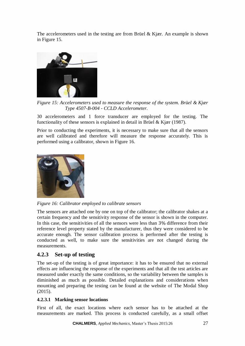
CHALMERS, Applied Mechanics, Master’s Thesis 2015:26 27
The accelerometers used in the testing are from Brüel & Kjær. An example is shown
in Figure 15.
Figure 15: Accelerometers used to measure the response of the system. Brüel & Kjær
Type 4507-B-004 - CCLD Accelerometer.
30 accelerometers and 1 force transducer are employed for the testing. The
functionality of these sensors is explained in detail in Brüel & Kjær (1987).
Prior to conducting the experiments, it is necessary to make sure that all the sensors
are well calibrated and therefore will measure the response accurately. This is
performed using a calibrator, shown in Figure 16.
Figure 16: Calibrator employed to calibrate sensors
The sensors are attached one by one on top of the calibrator; the calibrator shakes at a
certain frequency and the sensitivity response of the sensor is shown in the computer.
In this case, the sensitivities of all the sensors were less than 3% difference from their
reference level property stated by the manufacturer, thus they were considered to be
accurate enough. The sensor calibration process is performed after the testing is
conducted as well, to make sure the sensitivities are not changed during the
measurements.
4.2.3 Set-up of testing
The set-up of the testing is of great importance: it has to be ensured that no external
effects are influencing the response of the experiments and that all the test articles are
measured under exactly the same conditions, so the variability between the samples is
diminished as much as possible. Detailed explanations and considerations when
mounting and preparing the testing can be found at the website of The Modal Shop
(2015).
4.2.3.1 Marking sensor locations
First of all, the exact locations where each sensor has to be attached at the
measurements are marked. This process is conducted carefully, as a small offset

28 CHALMERS, Applied Mechanics, Master’s Thesis 2015:26
between the test articles can lead to significant differences in their responses.
Distances of the locations of the retained nodes with the EFI method in the FE-model
are taken to reference points that are easy to identify. These points are then marked in
the 3 tailgate objects as accurate as possible and the locations are numbered in the
same way as in the numerical model.
4.2.3.2 Set-up of test rig
A test rig located in the modal lab of VCC, as shown in Figure 17, is employed to
hang the tailgates to mimic the free support condition, see Section 2.5.2.
Figure 17: Set-up of the tailgate in the test rig
It is decided to hang the tailgate from the two upper holes shown in Figure 17. The
bars in the test rig are placed at the exact distance to cause the cords to lie completely
vertical when the tailgate is hanged; in this way, the rigid body modes of the system
will have as low frequency as possible. The cross-bars of the rig are strongly
tightened to avoid any motion during all the measurements.
Bungee cords are employed to hang the tailgate from the test rig: they are also
correctly tightened to ensure they will not move or loose. These cords are flexible to
reduce the eigenfrequencies of the rigid body modes. A thinner cord that is not as
flexible as the bungee cord is used to tie the bungee cords to the holes in the upper
part of the tailgate. These thinner cords are used to prevent resonances and damping
in the bungee cords to influence the response of the tailgate.
When the set-up of the test rig is accomplished, it is made sure that no loosing of the
employed cords will happen during the tests.
4.2.3.3 Attaching sensors and actuator
The sensors are connected to the cables, which in turn are connected to the frontend at
their other end. Special care is focused on connecting the sensors to the correct

CHALMERS, Applied Mechanics, Master’s Thesis 2015:26 29
channels in the frontend and numbering them accordingly thus they are attached to the
same locations as in the FE-model.
The accelerometers are attached into the tailgate utilising a silicone pistol: a thin layer
of warm glue is applied at the surface of the accelerometer and this is attached into the
marked location as fast as possible, before the glue cools down. The attachment is
conducted precisely so the accelerometer is placed exactly at the correct position and
the surface of the accelerometer is completely parallel to the surface of the tailgate.
Consequently, it is ensured that the response from the experiments will correspond to
the response of the FE-model at that point and exactly at the same direction. Each
time the accelerometers are placed into the system, it is ensured that the
accelerometers are securely fixed to the tailgate.
In order to prevent the cables of the accelerometers from influencing the damping of
the system during the experiments, the cables are attached into the test rig utilising
tape when possible. Consequently, when the accelerometers are attached to the
tailgate, the cables do not touch the tailgate. Besides, mounting the cables into the test
rig this way ensures that the set-up will be the same when measuring all the samples.
In the cases when it is not possible to prevent the cables from touching the system,
these are attached to the tailgate using tape to diminish damping.
The force transducer is attached into the tailgate employing a metal stud with a
threaded hole. A special glue type is utilised to attach the stud into the tailgate, i.e.
glue x60. This glue is obtained by mixing a powder with a liquid: the glue is applied
into one surface of the stud and this is pressed onto the desired excitation point of the
tailgate until the glue becomes stiff. This glue is much stiffer than the silicone
employed for the accelerometers, thus it is ensured that the connection will be strong
enough to prevent any movement when the excitation is applied.
The force transducer is then connected to the stud using a threaded metal rod: the rod
is screwed into the stud and then the transducer is screwed into the rod. In this way,
the force transducer is well tightened into the system.
Once all the sensors are attached to the system, the shaker is connected to the force
transducer. As previously mentioned in Section 4.2.2.2, this is conducted through the
stinger. If a stinger is not employed, any transversal load transmitted to the structure
from the exciter through the force transducer will be unmeasured but will still
contribute to vibration, resulting in an altered frequency response function. To
minimise this influence, the stinger is screwed into the actuator and is accurately
aligned to the threaded hole in the force transducer by varying the angle and the
height of the shaker. When everything is perfectly aligned, the exciter is fixed
strongly at that position and the stinger is partially screwed out of actuator,
introducing the other end into the force transducer. The plastic nuts are then used to
tighten the stinger with both the actuator and the force transducer.
During measurements, the driving point is always advisable to be measured, as
explained in The Modal Shop (2015). Hence, an accelerometer measuring the direct
accelerance of the system, i.e. the response of the vibration in the same point where
the input excitation is located, is used in the experiments, as shown in Figure 18.
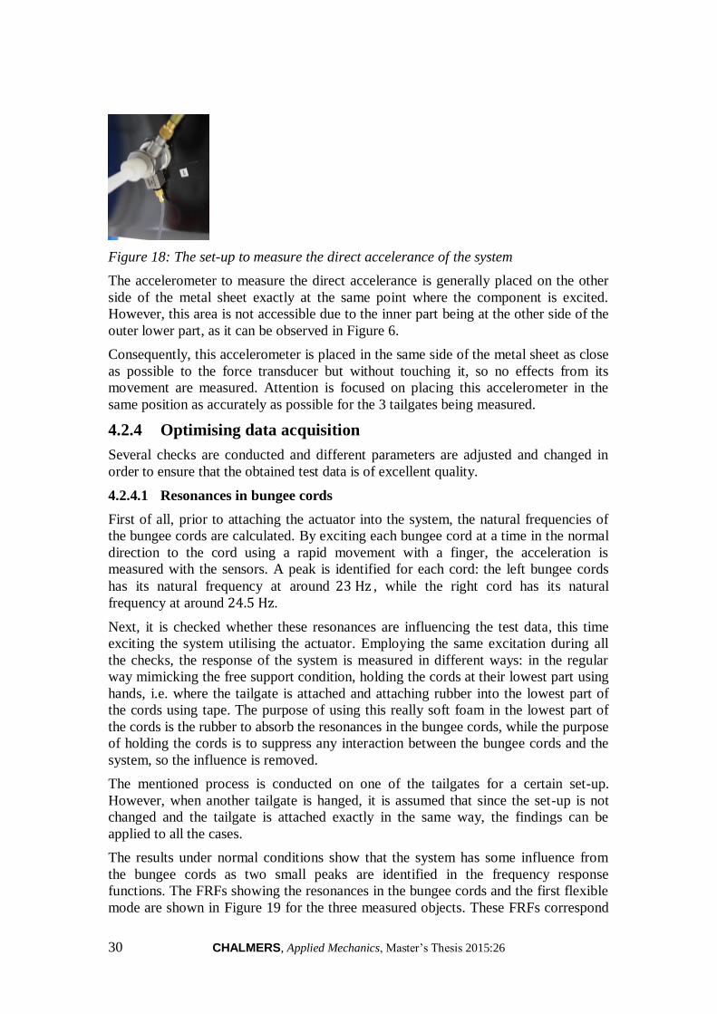
30 CHALMERS, Applied Mechanics, Master’s Thesis 2015:26
Figure 18: The set-up to measure the direct accelerance of the system
The accelerometer to measure the direct accelerance is generally placed on the other
side of the metal sheet exactly at the same point where the component is excited.
However, this area is not accessible due to the inner part being at the other side of the
outer lower part, as it can be observed in Figure 6.
Consequently, this accelerometer is placed in the same side of the metal sheet as close
as possible to the force transducer but without touching it, so no effects from its
movement are measured. Attention is focused on placing this accelerometer in the
same position as accurately as possible for the 3 tailgates being measured.
4.2.4 Optimising data acquisition
Several checks are conducted and different parameters are adjusted and changed in
order to ensure that the obtained test data is of excellent quality.
4.2.4.1 Resonances in bungee cords
First of all, prior to attaching the actuator into the system, the natural frequencies of
the bungee cords are calculated. By exciting each bungee cord at a time in the normal
direction to the cord using a rapid movement with a finger, the acceleration is
measured with the sensors. A peak is identified for each cord: the left bungee cords
has its natural frequency at around 23 Hz , while the right cord has its natural
frequency at around 24.5 Hz.
Next, it is checked whether these resonances are influencing the test data, this time
exciting the system utilising the actuator. Employing the same excitation during all
the checks, the response of the system is measured in different ways: in the regular
way mimicking the free support condition, holding the cords at their lowest part using
hands, i.e. where the tailgate is attached and attaching rubber into the lowest part of
the cords using tape. The purpose of using this really soft foam in the lowest part of
the cords is the rubber to absorb the resonances in the bungee cords, while the purpose
of holding the cords is to suppress any interaction between the bungee cords and the
system, so the influence is removed.
The mentioned process is conducted on one of the tailgates for a certain set-up.
However, when another tailgate is hanged, it is assumed that since the set-up is not
changed and the tailgate is attached exactly in the same way, the findings can be
applied to all the cases.
The results under normal conditions show that the system has some influence from
the bungee cords as two small peaks are identified in the frequency response
functions. The FRFs showing the resonances in the bungee cords and the first flexible
mode are shown in Figure 19 for the three measured objects. These FRFs correspond
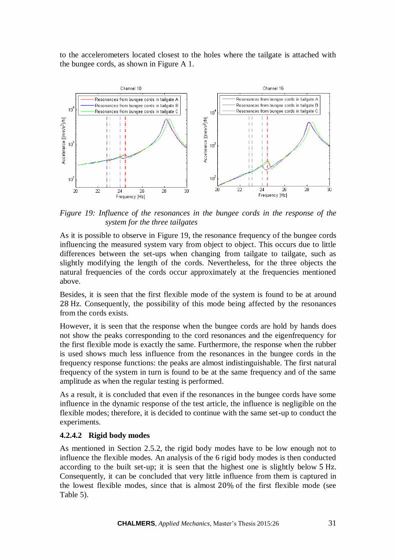
CHALMERS, Applied Mechanics, Master’s Thesis 2015:26 31
to the accelerometers located closest to the holes where the tailgate is attached with
the bungee cords, as shown in Figure A 1.
Figure 19: Influence of the resonances in the bungee cords in the response of the
system for the three tailgates
As it is possible to observe in Figure 19, the resonance frequency of the bungee cords
influencing the measured system vary from object to object. This occurs due to little
differences between the set-ups when changing from tailgate to tailgate, such as
slightly modifying the length of the cords. Nevertheless, for the three objects the
natural frequencies of the cords occur approximately at the frequencies mentioned
above.
Besides, it is seen that the first flexible mode of the system is found to be at around
28 Hz. Consequently, the possibility of this mode being affected by the resonances
from the cords exists.
However, it is seen that the response when the bungee cords are hold by hands does
not show the peaks corresponding to the cord resonances and the eigenfrequency for
the first flexible mode is exactly the same. Furthermore, the response when the rubber
is used shows much less influence from the resonances in the bungee cords in the
frequency response functions: the peaks are almost indistinguishable. The first natural
frequency of the system in turn is found to be at the same frequency and of the same
amplitude as when the regular testing is performed.
As a result, it is concluded that even if the resonances in the bungee cords have some
influence in the dynamic response of the test article, the influence is negligible on the
flexible modes; therefore, it is decided to continue with the same set-up to conduct the
experiments.
4.2.4.2 Rigid body modes
As mentioned in Section 2.5.2, the rigid body modes have to be low enough not to
influence the flexible modes. An analysis of the 6 rigid body modes is then conducted
according to the built set-up; it is seen that the highest one is slightly below 5 Hz.
Consequently, it can be concluded that very little influence from them is captured in
the lowest flexible modes, since that is almost 20% of the first flexible mode (see
Table 5).
32 CHALMERS, Applied Mechanics, Master’s Thesis 2015:26
4.2.4.3 Best actuator location
The actuator is first tried to be placed at the optimal location according to the
balanced realization accomplished in Section 4.1.1, as shown in Table 2. However,
when the shaker is attached in point a shown in Figure 9 and the response of the
system is measured, it is seen that the system is rattling a lot, i.e. metal panels
composing the tailgate are touching each other during the vibration. Rattling leads to
non-linear response of the system. This has to be prevented as it is not possible to
calibrate the FE-model based on non-linear response of the structure.
The reason for rattling when the actuator is attached at this location is considered. It is
seen that the inner part and outer upper part of the tailgate are really close to each
other in this actuator location, as it is possible to understand from Figure 6. Hence, it
is assumed that when the excitation if applied at this point in the outer upper part and
the panel starts to vibrate, this panel touches the inner one.
Consequently, it is determined to change the actuator position. Considering the
second best option, it is seen that the actuator is located at the wiper motor bracket;
see point b in Figure 9.
During the previous tests, it was possible to realise that this is a critical part in the
vibration testing. It can be observed in Figure 6 that the inner part, the outer upper
part and the wiper motor bracket are connected in one area which is not totally well
aligned, i.e. a welded surface of the wiper motor bracket is not completely parallel to
the connected inner part. It is believed that this fact leads to rattling also in this area of
the system. Apart from that, the wiper motor bracket is a rather small part compared
to the other components, which is attached using spot welds. Some variability can
then be expected in between the test articles, or at least potential for variability is
higher than in other areas of the structure.
As a result, it is determined not to use this second best actuator location. The shaker is
therefore placed at the third most optimal option, i.e. at the middle of the outer lower
part, named point c in Figure 9. The response is found to be linear when this actuator
location is utilised.
4.2.4.4 Length of stinger
Different lengths of the stinger are considered when the shaker is attached to the
tailgate. This is done in order to avoid the problems mentioned in Section 2.5.2. It is
decided to test using a stinger long enough to observe a slight bending when just
pressing it with a fingertip. However, it cannot be too long so buckling occurs during
the excitation. A balance needs to be struck by lengthening and shortening the stinger
and making sure the obtained response is exactly the same for varying lengths. From
this study a stinger length is decided and the resulting configuration can be seen in
Figure 13.
4.2.4.5 Avoid rattling in the system
As previously mentioned, there are some areas of the system where there is potential
for rattling. This is mainly expected in the area where the wiper motor bracket is
connected into the panels and in the upper reinforced part, i.e. where the upper
reinforcements, the inner part and the outer upper part are connected.

CHALMERS, Applied Mechanics, Master’s Thesis 2015:26 33
Consequently, it is determined to prevent rattling from occurring by adding
instruments such that the parts are more tightly connected to or better separated from
each other. In the first case, a tiny stick of wood is inserted in the groove between the
inner part and the wiper motor bracket mentioned in Section 4.2.4.3, as shown in
Figure 20.
Figure 20: Wiper motor bracket with a wooden stick inserted in the groove
This stick is not influencing the response, as only negligible mass or stiffness is
added, but just prevents rattling occurring between the parts.
To prevent rattling in the upper reinforced part, 4 screws are added to tighten the
connection between the inner part and the upper reinforcements, as shown in Figure
21.
Figure 21: Side of the tailgate set-up showing the added screws
To compensate for the added mass and stiffness in the simulations, the screws also
have to be included in the FE-model.
4.2.4.6 Capture mode 4
In the pre-test planning, when the eigenmodes of the FE-model are investigated, it is
observed that the motion of mode number four occur mainly in the same plane as the
tailgate, as it is mainly a shearing mode. The shape of this mode can be observed in
Figure 22.
Added screws
Wooden stick

34 CHALMERS, Applied Mechanics, Master’s Thesis 2015:26
Figure 22: Shape of mode 4 according to nominal FE-model. Shape of mesh when the
tailgate is not deformed shown in yellow.
On the other hand, all the accelerometers are approximately located perpendicular to
this plane, i.e. in the out-of-plane direction of the tailgate. Hence, it is observed that
this mode is not well captured by the accelerometers in the testing.
Consequently, it is decided to change the location of one accelerometer and place it at
an area where the motion of mode four is strong, as shown in Figure 22. The changed
accelerometer is number 29 according to the EFI method, so it is one of the points
adding less information to the Fisher information matrix, thus it is thought that not
much information about the dynamics of the system will be lost by this modification.
The location of the accelerometer is also shown in Figure A 1.
4.2.5 System excitation
As previously mentioned, two types of excitation strategies are used in the
measurements; burst-random testing and stepped-sine testing, see Section 2.5.3. With
both strategies the tailgates are measured in the frequency range between 10 to
400 Hz.
One thing to take into account when measuring is the sampling strategy for the
discrete frequencies that are selected for frequency response function evaluation. The
half-band width of a damped structural resonance depends of the frequency and the
relative modal damping, as explained in Abrahamsson (2012). Hence, the half-band
width increases linearly with increasing resonance frequency, thus it is advisable to
use frequency steps that increase linearly with frequency; in this way, it is possible to
have a constant number of samples over the half-band width of all the measured
resonances.
An effective way to evaluate the sampling strategy employed in vibration testing
consists in looking at the Nyquist plot, as explained in McConnell (1995). This plot
shows the real part of the measured transfer function versus the imaginary part. The
number of measured samples should be high enough so each mode represented by a
circle in the Nyquist plot is correctly defined, but not too high because the testing time
is then too long. The Nyquist plot is therefore checked with both strategies to ensure
that a balance in the number of samples is obtained.
Attention is also focused in the maximum voltage that the sensors can measure. It is
known that the accelerometers do not work properly when converting the sensed
New accelerometer location
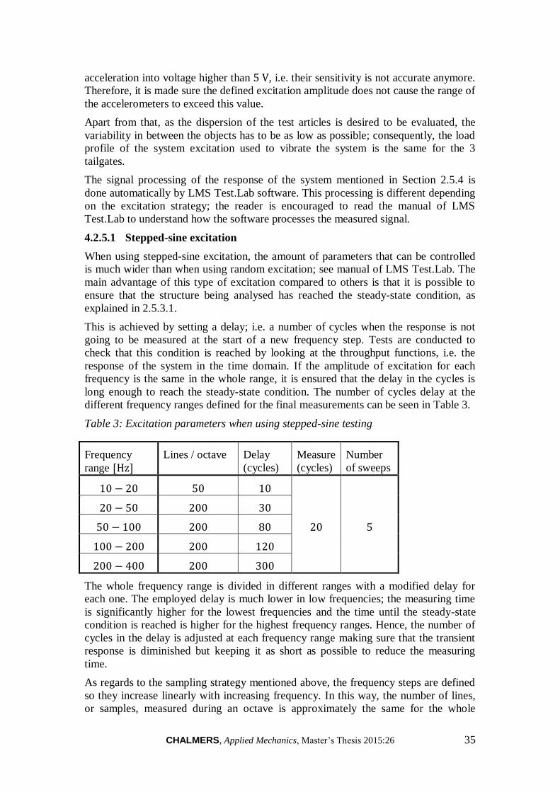
CHALMERS, Applied Mechanics, Master’s Thesis 2015:26 35
acceleration into voltage higher than 5 V, i.e. their sensitivity is not accurate anymore.
Therefore, it is made sure the defined excitation amplitude does not cause the range of
the accelerometers to exceed this value.
Apart from that, as the dispersion of the test articles is desired to be evaluated, the
variability in between the objects has to be as low as possible; consequently, the load
profile of the system excitation used to vibrate the system is the same for the 3
tailgates.
The signal processing of the response of the system mentioned in Section 2.5.4 is
done automatically by LMS Test.Lab software. This processing is different depending
on the excitation strategy; the reader is encouraged to read the manual of LMS
Test.Lab to understand how the software processes the measured signal.
4.2.5.1 Stepped-sine excitation
When using stepped-sine excitation, the amount of parameters that can be controlled
is much wider than when using random excitation; see manual of LMS Test.Lab. The
main advantage of this type of excitation compared to others is that it is possible to
ensure that the structure being analysed has reached the steady-state condition, as
explained in 2.5.3.1.
This is achieved by setting a delay; i.e. a number of cycles when the response is not
going to be measured at the start of a new frequency step. Tests are conducted to
check that this condition is reached by looking at the throughput functions, i.e. the
response of the system in the time domain. If the amplitude of excitation for each
frequency is the same in the whole range, it is ensured that the delay in the cycles is
long enough to reach the steady-state condition. The number of cycles delay at the
different frequency ranges defined for the final measurements can be seen in Table 3.
Table 3: Excitation parameters when using stepped-sine testing
Frequency
range [Hz] Lines / octave Delay
(cycles)
Measure
(cycles)
Number
of sweeps
10 − 20 50 10
20 5
20 − 50 200 30
50 − 100 200 80
100 − 200 200 120
200 − 400 200 300
The whole frequency range is divided in different ranges with a modified delay for
each one. The employed delay is much lower in low frequencies; the measuring time
is significantly higher for the lowest frequencies and the time until the steady-state
condition is reached is higher for the highest frequency ranges. Hence, the number of
cycles in the delay is adjusted at each frequency range making sure that the transient
response is diminished but keeping it as short as possible to reduce the measuring
time.
As regards to the sampling strategy mentioned above, the frequency steps are defined
so they increase linearly with increasing frequency. In this way, the number of lines,
or samples, measured during an octave is approximately the same for the whole
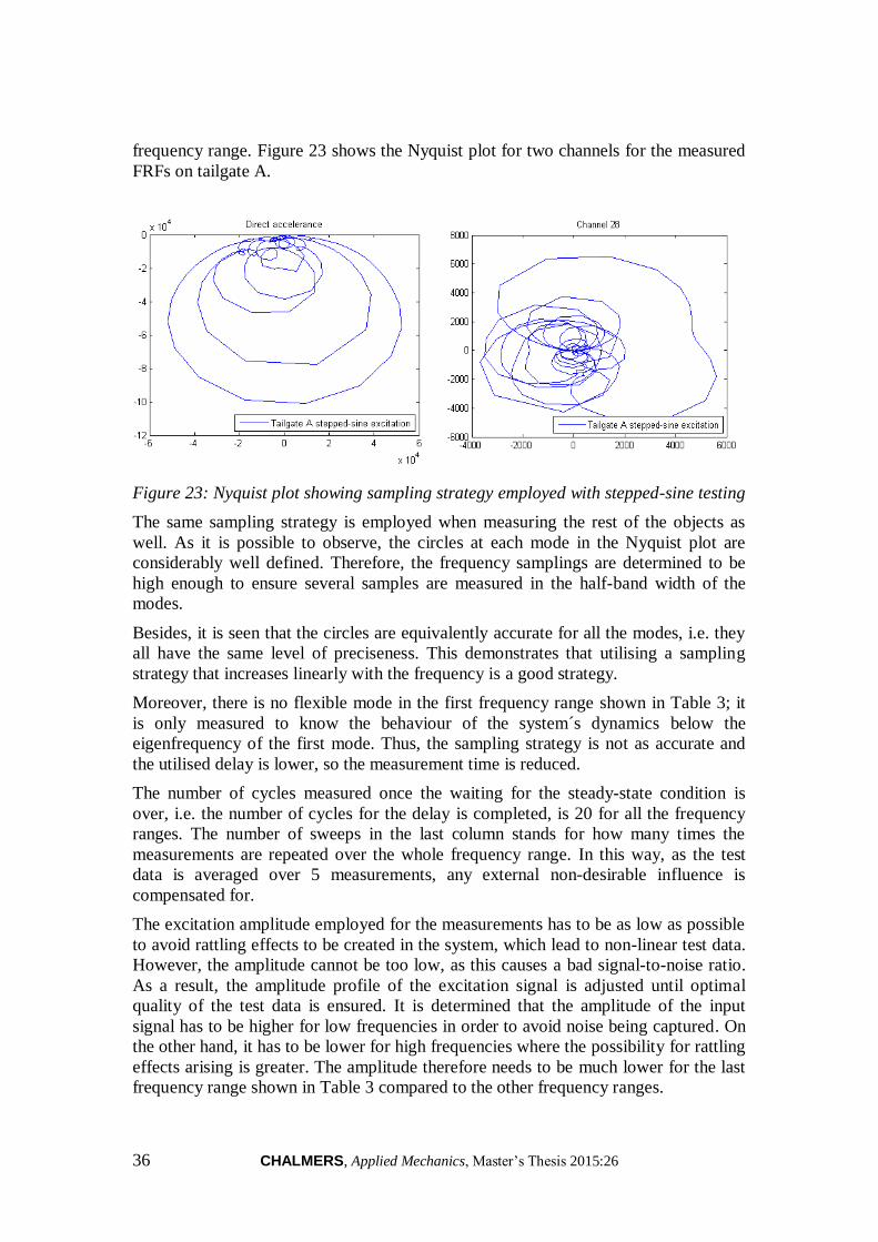
36 CHALMERS, Applied Mechanics, Master’s Thesis 2015:26
frequency range. Figure 23 shows the Nyquist plot for two channels for the measured
FRFs on tailgate A.
Figure 23: Nyquist plot showing sampling strategy employed with stepped-sine testing
The same sampling strategy is employed when measuring the rest of the objects as
well. As it is possible to observe, the circles at each mode in the Nyquist plot are
considerably well defined. Therefore, the frequency samplings are determined to be
high enough to ensure several samples are measured in the half-band width of the
modes.
Besides, it is seen that the circles are equivalently accurate for all the modes, i.e. they
all have the same level of preciseness. This demonstrates that utilising a sampling
strategy that increases linearly with the frequency is a good strategy.
Moreover, there is no flexible mode in the first frequency range shown in Table 3; it
is only measured to know the behaviour of the system´s dynamics below the
eigenfrequency of the first mode. Thus, the sampling strategy is not as accurate and
the utilised delay is lower, so the measurement time is reduced.
The number of cycles measured once the waiting for the steady-state condition is
over, i.e. the number of cycles for the delay is completed, is 20 for all the frequency
ranges. The number of sweeps in the last column stands for how many times the
measurements are repeated over the whole frequency range. In this way, as the test
data is averaged over 5 measurements, any external non-desirable influence is
compensated for.
The excitation amplitude employed for the measurements has to be as low as possible
to avoid rattling effects to be created in the system, which lead to non-linear test data.
However, the amplitude cannot be too low, as this causes a bad signal-to-noise ratio.
As a result, the amplitude profile of the excitation signal is adjusted until optimal
quality of the test data is ensured. It is determined that the amplitude of the input
signal has to be higher for low frequencies in order to avoid noise being captured. On
the other hand, it has to be lower for high frequencies where the possibility for rattling
effects arising is greater. The amplitude therefore needs to be much lower for the last
frequency range shown in Table 3 compared to the other frequency ranges.

CHALMERS, Applied Mechanics, Master’s Thesis 2015:26 37
Besides, the LMS Test.Lab software provides the opportunity of adjusting the
amplitude of the input signal depending on the energy the system requires at each
frequency step. This option is used and therefore the energy input is increased in the
range of anti-resonances and decreased in the range of resonances.
Finally, the measurements are repeated varying the profile of the reference amplitude.
The result of varying the stimuli strengths is shown in Figure 24.
Figure 24: FRFs measured on tailgate A with varying amplitude to evaluate the
linearity of the response of the object
The figure shows the FRFs obtained from measurements on tailgate A utilising the
optimised amplitude profile mentioned above. The measurements are repeated on the
same object doubling and halving the profile of the amplitude, also shown in Figure
24. It is possible to observe that the FRFs obtained for different amplitudes show no
significant differences.
The amplitude variation is also performed on the other two objects, obtaining exactly
the same results for different magnitudes of the signal. Consequently, it is ensured
that the system behaves sufficiently linearly under the defined system excitation
profile for the three tested articles.
4.2.5.2 Burst-random excitation
When this excitation signal is employed the parameters to be controlled are more
restricted. Due to this excitation type being substantially much faster, the used
sampling strategy is the same for all the frequency ranges: a resolution of 0.05 Hz is
utilised.
As mentioned above, the amplitude of excitation has to be decreasing for increasing
frequency. Consequently, pink noise is employed; i.e. the power spectral density or
energy utilised is inversely proportional to the frequency of the signal, thus each
octave in the frequency range contains the same amount of input energy.
The amplitude of excitation is also lowered as much as possible when measuring the
system using burst-random signal, but making sure that noise influence the test data as
little as possible. Different amplitudes are used as well to ensure the system is
sufficiently linear at all frequencies.
20 averages are utilised during the measurements, meaning that the period with
random excitation is repeated and averages of the results are taken. The shaker is
sending signal into the system 60% of the time during each period, while it is silent
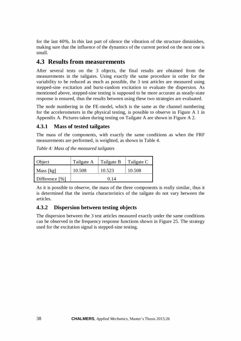
38 CHALMERS, Applied Mechanics, Master’s Thesis 2015:26
for the last 40%. In this last part of silence the vibration of the structure diminishes,
making sure that the influence of the dynamics of the current period on the next one is
small.
4.3 Results from measurements
After several tests on the 3 objects, the final results are obtained from the
measurements in the tailgates. Using exactly the same procedure in order for the
variability to be reduced as much as possible, the 3 test articles are measured using
stepped-sine excitation and burst-random excitation to evaluate the dispersion. As
mentioned above, stepped-sine testing is supposed to be more accurate as steady-state
response is ensured, thus the results between using these two strategies are evaluated.
The node numbering in the FE-model, which is the same as the channel numbering
for the accelerometers in the physical testing, is possible to observe in Figure A 1 in
Appendix A. Pictures taken during testing on Tailgate A are shown in Figure A 2.
4.3.1 Mass of tested tailgates
The mass of the components, with exactly the same conditions as when the FRF
measurements are performed, is weighted, as shown in Table 4.
Table 4: Mass of the measured tailgates
Object Tailgate A Tailgate B Tailgate C
Mass [kg] 10.508 10.523 10.508
Difference [%] 0.14
As it is possible to observe, the mass of the three components is really similar, thus it
is determined that the inertia characteristics of the tailgate do not vary between the
articles.
4.3.2 Dispersion between testing objects
The dispersion between the 3 test articles measured exactly under the same conditions
can be observed in the frequency response functions shown in Figure 25. The strategy
used for the excitation signal is stepped-sine testing.

CHALMERS, Applied Mechanics, Master’s Thesis 2015:26 39
Figure 25: Dispersion between 3 test articles measured employing stepped-sine
excitation
The FRFs for the rest of the points measured during the experiments are shown in
Figure B 1 in Appendix B.
As it is possible to observe in Figure 25, the dispersion between the articles is very
low in the frequency range up to approximately 200 Hz, whereas the curves are
extremely similar for the first 5 flexible modes. In this range it is seen that tailgate C
is a little bit less stiff than the other two components in the area around 150 Hz that
contains a significant mode, and there is some dispersion between them in the range
close to 200 Hz.
The dispersion is significant in the frequency range between 220 − 280 Hz , the
variability between the objects diminishes in the range close to 300 Hz and it
becomes obvious again in frequencies higher than 340 Hz.
Summarising, it is concluded that some dispersion exists between the tested articles
even if the complexity of the components is not high. Nevertheless, for the first
flexible modes lower than 200 Hz in eigenfrequencies, the FRFs show good
correlation.
In this frequency range, an evaluation of the eigenfrequencies is conducted, as it is
possible to observe in Table 5.

40 CHALMERS, Applied Mechanics, Master’s Thesis 2015:26
Table 5: Dispersion in identified eigenfrequencies in between 3 measured tailgates
Frequency
range [Hz] Mode
number
Eigenfreq.
tailgate A
[Hz]
Eigenfreq.
tailgate B
[Hz]
Eigenfreq.
tailgate C
[Hz]
Highest
deviation
[Hz]
Highest
difference
[%]
10-60 1 28.2 28.2 28.2 0.0
0.7 2 56.1 56.4 56.5 0.4
60-100
3 77.9 78.5 79.4 1.5
1.9 4 91.3 91.7 92.5 1.2
5 97.3 98.3 98.6 1.3
100-156
6 118.1 119.5 120.7 2.6
2.3 7 135.5 136.5 138.7 3.2
8 142.1 139.7 142.8 3.1
9 155.7 153.5 155.9 2.4
156-200
10 159.4 159.4 157.9 1.5
1.0
11 171.7 172.1 173.4 1.7
12 181.1 184.1 181.5 3.0
13 186.3 186.8 185.8 1.0
14 191.6 192.4 192.3 0.8
As it is possible to see, the eigenfrequencies of the system in the frequency range 0 −200 Hz show very good correlation when comparing the 3 tested articles; especially
the first 2 modes are extremely well correlated.
If attention is focused on frequency ranges higher than 200 Hz, it is seen that the
dispersion between the objects is large at these frequencies and therefore it is not
meaningful to identify and compare the eigenfrequencies of the modes.
An analysis of the dissipative energy in the system, i.e. damping effect, is also
accomplished, shown in Table 6.
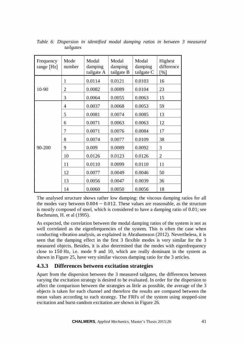
CHALMERS, Applied Mechanics, Master’s Thesis 2015:26 41
Table 6: Dispersion in identified modal damping ratios in between 3 measured
tailgates
Frequency
range [Hz] Mode
number
Modal
damping
tailgate A
Modal
damping
tailgate B
Modal
damping
tailgate C
Highest
difference
[%]
10-90
1 0.0114 0.0121 0.0103 16
2 0.0082 0.0089 0.0104 23
3 0.0064 0.0055 0.0063 15
90-200
4 0.0037 0.0068 0.0053 59
5 0.0081 0.0074 0.0085 13
6 0.0071 0.0063 0.0063 12
7 0.0071 0.0076 0.0084 17
8 0.0074 0.0077 0.0109 38
9 0.009 0.0089 0.0092 3
10 0.0126 0.0123 0.0126 2
11 0.0110 0.0099 0.0110 11
12 0.0077 0.0049 0.0046 50
13 0.0056 0.0047 0.0039 36
14 0.0060 0.0050 0.0056 18
The analysed structure shows rather low damping: the viscous damping ratios for all
the modes vary between 0.004 − 0.012. These values are reasonable, as the structure
is mostly composed of steel, which is considered to have a damping ratio of 0.01; see
Bachmann, H. et al (1995).
As expected, the correlation between the modal damping ratios of the system is not as
well correlated as the eigenfrequencies of the system. This is often the case when
conducting vibration analysis, as explained in Abrahamsson (2012). Nevertheless, it is
seen that the damping effect in the first 3 flexible modes is very similar for the 3
measured objects. Besides, it is also determined that the modes with eigenfrequency
close to 150 Hz, i.e. mode 9 and 10, which are really dominant in the system as
shown in Figure 25, have very similar viscous damping ratio for the 3 articles.
4.3.3 Differences between excitation strategies
Apart from the dispersion between the 3 measured tailgates, the differences between
varying the excitation strategy is desired to be evaluated. In order for the dispersion to
affect the comparison between the strategies as little as possible, the average of the 3
objects is taken for each channel and therefore the results are compared between the
mean values according to each strategy. The FRFs of the system using stepped-sine
excitation and burst-random excitation are shown in Figure 26.

42 CHALMERS, Applied Mechanics, Master’s Thesis 2015:26
Figure 26: Differences between FRFs showing mean of 3 test articles measured using
two excitation strategies
More FRFs showing the influence between using stepped-sine or burst-random
excitation are shown in Figure B 2 in Appendix B.
As it is possible to observe, even if tiny differences are observed between the two
excitation strategies, the measured FRFs are very similar. In the FRFs in the upper
plots of Figure 26 corresponding to direct accelerance and to the average over all the
measured channels, it is almost not possible to perceive the difference between the
strategies.
On the other hand, if attention is focused on the FRFs shown in the lower plots of
Figure 26, it is seen that in the highlighted areas the response of the system is
different depending on the excitation signal.
The main differences between the excitation types are seen in the anti-resonances.
However, some variation can also be observed in the resonances; i.e. peaks for some
of the modes do not show the same amplitude when the signal corresponds to stepped-
sine compared to when burst-random excitation is employed. The reason for this
could be that whereas the response is ensured to be steady-state when stepped-sine
excitation is utilised, it is possible that the response is still not fully periodic for some
of the modes when the vibration is recorded using random noise. Therefore, it is

CHALMERS, Applied Mechanics, Master’s Thesis 2015:26 43
concluded that stepped-sine testing provides higher accuracy in the vibrational
response of the system.
On the other hand, if the difference between employing these two strategies is
compared to the dispersion in the response of the different articles, it is seen that the
variation between the measured tailgates is more significant than the dissimilarities
obtained with the two signals.
44 CHALMERS, Applied Mechanics, Master’s Thesis 2015:26
5 FE-model vs test data
Once accurate test data is available describing the vibrations of the physical tailgate, it
is possible to compare the dynamics of the real system with the response obtained
from the FE-model. Calibration of the numerical model is then possible to conduct so
the model resembles reality as exactly as possible.
Due to the reasons explained in Section 4.3.2, it is decided to conduct the calibration
process in the frequency range between 10 − 200 Hz. It is concluded that there is no
point in employing higher frequencies. The calibration process with FEMcali is to be
conducted against one of the measured objects; hence, considering the dispersion
between the tailgates at high frequencies shown in Figure 25, the FE-model would be
calibrated against one of the objects, as the other objects are not similar at these
frequencies. This would cause that the simulations would not be a representation of
the physical tailgate, but just would represent one of the measured objects in case the
calibration is performed in high frequencies.
5.1 System identification on test data
As mentioned in Section 2.6, system identification is performed in the test data in
order to obtain a state-space model representing the physical tailgates. The identified
system has to be as similar as possible to the raw test data to perform the calibration
of the FE-model with respect to an accurate representation of reality.
It is determined to utilise test data obtained from tailgate A to conduct this process,
since the response of this object is the one that best describes the mean of the
dynamics of the 3 measured components; i.e. looking at the FRFs in Figure 25, it is
seen that the curve for this object is the closest one to the other two. Hence, the
system identification is accomplished on the experiments obtained from tailgate A in
the frequency range 10 − 195 Hz. The last 5 Hz range is removed in order not to
identify non-existent modes at these frequencies.
The system identification procedure is performed using the n4sid function from the
System Identification toolbox of MATLAB. In order to optimise the identified state-
space model, different features have to be taken into account.
5.1.1 Remove influence from bungee-cords
When the process of system identification is started, it is seen that the little peaks
corresponding to the natural frequencies of the bungee cords measured in the response
of the object have to be removed. Even if the influence of these resonances affecting
the structure is considerably low, these peaks are captured in all the accelerometers;
therefore, they could by mistake be identified as flexible modes of the system. As a
result, the test data in the frequency range 23 − 27.5 Hz is removed to conduct the
system identification.
5.1.2 Mobility data
It is known that depending on the type of data used for the system identification
procedure, more attention is focused on different areas in the frequency range; while
accelerance data tends to identify more modes in high frequencies, low frequencies
would be considered more significant if receptance data is used, as explained in
Abrahamsson (2012).
CHALMERS, Applied Mechanics, Master’s Thesis 2015:26 45
After checking the results varying the type of test data, it is determined that mobility
data leads to the most accurate representation of the measured data. This raw data
consists in frequency response functions of accelerance type, thus represents the
acceleration sensed in the system per unit force. Hence, mobility transfer functions are
obtained from the measured accelerance transfer functions as;
Accelerance: �̂� = 𝐇 �̂�
Mobility: �̂� = 𝐘 �̂�
�̂� = 𝑖𝝎 �̂� → �̂� =�̂�
𝑖𝝎=
𝐇
𝑖𝝎 �̂� → 𝐘 =
𝐇
𝑖𝝎
(5)
System identification is then performed utilising mobility data, i.e. data relating
velocity per unit force, rather than using accelerance data.
5.1.3 Frequency response data object
In order for the n4sid function to process the measured data, this has to be prepared.
The data obtained from the LMS Test.Lab software consists in one vector per channel
containing the response of the system for each measured frequency step in a complex
number format. This data is converted in MATLAB into a multidimensional array
response.
A Frequency Response Data (FRD) model object is then created in MATLAB
employing the response and the vector containing the measured frequency steps. The
idfrd function is employed for that.
5.1.4 Model order estimation
The only variable the N4SID algorithm requires to be given is the model order to
identify a state-space model. As mentioned in Section 2.6, this order represents the
number of state variables the frequency range of interest contains. The state-space
representation, which is a representation of the second order equation of motion as
stated in 2.2, consists in two first order equations. Therefore, the state-space
representation is of second order, i.e. its model order is two for each state variable that
it contains. Consequently, the state-space model order is defined by the number of
modes that are captured in the interested frequency range times two.
The FE-model contains 15 eigenmodes in the frequency interval mentioned above and
approximately 15 peaks are also counted in the test data; hence, a model order of 30 is
employed as a starting point.
An eigenvalue analysis of the identified state-space model is made and the
eigenvalues 𝜆𝑛 and eigenvectors corresponding to the measured data are obtained
from this analysis, as explained in Abrahamsson (2012). This is accomplished by
solving the state-space coefficient matrix 𝐀, shown in Section 2.2.2.
Hence, the eigenfrequencies and the modal damping ratios of the eigenmodes, shown
in Table 5 and Table 6, respectively, are calculated according to;
𝑓𝑛 =𝐼𝑚(𝜆𝑛)
2𝜋 [Hz]
𝜉𝑛 = −𝑅𝑒(𝜆𝑛)
𝐼𝑚(𝜆𝑛)
(6)
46 CHALMERS, Applied Mechanics, Master’s Thesis 2015:26
Besides, as mentioned in Section 2.7.1, the MAC correlation can be utilised to
evaluate the identified model by comparing the eigenvector angles between the test
data and the FE-model as;
𝑀𝐴𝐶(𝜌𝑖𝑥 , 𝜌𝑗
𝐴) =((𝜌𝑖
𝑥)𝑇𝜌𝑗𝐴)
|𝜌𝑖𝑥|
2|𝜌𝑗
𝐴|2 (7)
The eigenvectors that correspond to the virtual accelerometer locations in the FE-
model 𝜌𝑗𝐴 are extracted from the FE software by an eigenvalue analysis. On the other
hand, the eigenvectors of the tested tailgate for the points where the accelerometers
are placed 𝜌𝑖𝑥 are obtained by a similarity transformation on the state-space model
according to 𝒙 = 𝐏𝒛 . The corresponding columns of the obtained state-space
coefficient matrix 𝐂 = 𝐂𝐏 , the columns of C̅.𝑖, belong to the decoupled state 𝑧𝑖; i.e.
each column is the eigenvector of the i:th state as seen by the sensors.
According to Abrahamsson (2012), mode pairs from test and FE data giving a MAC
number higher than 0.95 are considered to be closely correlated, whereas a number
lower than 0.8 should indicate that the modes are poorly correlated. In the system
identification process, the MAC correlation is calculated using the nominal FE-model.
This model is then calibrated in order to further improve its prediction capability;
hence, really high correlation numbers are not expected for the nominal model.
By comparing the eigenfrequencies and the MAC correlation numbers of each mode
from the test data with the FE-model, it is seen that when a model order of 30 is
employed, mode 4 in the FE-model is not captured in the identified state-space model
containing 15 state variables, i.e. eigenmodes. It is then determined that changing the
location of accelerometer 29 in the experiments in order to capture this mode, as
mentioned in Section 4.2.4.6, was not enough to get the influence of this mode, i.e.
peaks created by the influence of noise in the measurements are identified as modes
before the resonance corresponding to the 4th mode.
Otherwise, it is concluded that this mode exists in the real components, as a peak can
be observed for some of the measured channels in the frequency range where the
simulations pointed out that this mode should lie. An analysis of this mode shows
that, due to its eigenvector shape and the non-optimal accelerometer placement to
observe this mode mentioned in Section 4.2.4.6, a potential for not completely
capturing this mode by the present test set-up exists. Besides, the actuator is located
perpendicular to the direction of vibration of the system under this eigenmode,
restricting the free vibration of the system; i.e. as the shaker is fixed to the ground
during the experiments and strongly attached to the tailgate, vibration in the direction
of the stinger is freely allowed, but motion in the plane perpendicular to the rod is
possibly restricted. On the other hand, no such restrictions exist in the FE-model;
hence, it is thought that the 4th flexible mode may be as present as in the FE-model in
the physical object, but the set-up of the testing resulted in not being optimised to
control and observe this mode.
As a result, it is decided to increase the model order during the system identification.
It is required to increase it up to 40 in order to better identify mode 4. The MAC
correlation is repeated with the newly identified state-space model containing mode 4

CHALMERS, Applied Mechanics, Master’s Thesis 2015:26 47
and a MAC index of 0.773 is calculated for this mode. Then, it is determined that
even if the shapes of the eigenvectors have some similarities, this mode pair shows
poor correlation.
Nevertheless, if only the channels where a peak for mode 4 is observed are taken, the
correlation index increases; using the 10 channels where the peak is most obvious the
index results to be 0.96 , while employing 17 channels were the peaks can be
recognised gives an index of 0.94. The MAC index for this mode is also calculated
for the other two measured tailgates utilising all the channels: for tailgate B the index
is 0.84, while the index is 0.8 for tailgate C. Consequently, it is decided that mode 4
exists in the physical objects and has to some extent been captured in the
measurements.
Furthermore, it is necessary to take into account that, since the FE-model employed is
the nominal one, the somewhat small MAC indices could be caused by the FE-model
not representing the test data accurately enough rather than insisting that mode 4 does
not exist in the test objects.
Finally, using a high model order lead to spurious modes to be identified and included
in the created state-space model. A model order of 40 lead to 20 identified state
variables: while 14 eigenmodes are assumed to be real natural frequencies of the
system, the remaining 6 are determined to be fictitious modes. These eigenmodes are
shown in Table 5 and Table 6, where the spurious modes are omitted.
Nevertheless, these spurious modes are just duplicating the real resonances, i.e. they
are identified really close to eigenfrequencies of other physical modes. For instance,
mode 1 with an eigenfrequency of 28.2 Hz is mirrored by a spurious mode with an
eigenfrequency of 28 Hz. The same behaviour is repeated for mode 2, 5, 7, 12 and 13.
It is then seen that these spurious modes are not affecting either the results of the
eigenvalue analysis or the FRD object created from the identified state-space model.
Besides, as the calibration procedure is based on the deviation metric, which is
calculated employing the frequency response functions, and since the fictitious modes
are not influencing the FRFs, it is assumed that the calibration is not affected by them.
Due to all the reasons mentioned above, it is decided to conduct the system
identification process with the somewhat excessive model order of 40.
5.1.5 State-space model inflation
The N4SID algorithm creates a state-space model based on the peaks that it identifies
as eigenmodes of the system in the frequency range of the FRD object employed as
input. However, this model contains no information about how the system behaves in
frequencies out of the range of interest; the lower and upper frequency range bounds
of the identified system are therefore generally not accurate representation of the raw
test data.
As a result, the state-space model is inflated utilising poles: one pseudo rigid body
mode and one high frequency mode are included in the identified system. This
process is conducted employing ssinflate function in MATLAB, developed for
FEMcali toolbox by Abrahamsson and Kammer (2015). The function requires the
FRD object from test data and the identified model out of this data, apart from the
poles desired to be added.
In order for the model to have a better fit to the measured data, poles at different
frequencies are considered. The best option is calculated using the deviation metric
48 CHALMERS, Applied Mechanics, Master’s Thesis 2015:26
between the inflated model and the raw test data to evaluate the considered poles.
Employing a pseudo rigid body mode at 0.1 Hz and a high frequency residual mode at
220 Hz resulted in the minimisation of the deviation metric.
Furthermore, the state-space coefficient matrices 𝐁 and 𝐂 are re-estimated to optimise
the identified state-space model by least-square fitting to raw test data. This is also
done employing functions developed for FEMcali: ff2best for the 𝐁 matrix and ff2cest
for the 𝐂 matrix, respectively. The least-square fitting procedure requires the
identified and inflated state-space model and the FRD object of this model.
5.1.6 State-space model vs raw test data
After the whole process is conducted, a state-space model that is an extremely
accurate representation of the measured data in the experiments on tailgate A is
obtained.
Nevertheless, this state-space model represents mobility data; since the FEMcali
toolbox is prepared to work with accelerance data, the state-space model is
transformed to mobility data.
If attention is focused on Section 2.2.2, looking at equation (3) it is seen that the
output equation gives velocity 𝒚(𝒕) = �̇�(𝒕) . Hence, the state-space model
representing accelerance data is calculated as;
Current model: {�̇�(𝒕) = 𝐀𝒙(𝒕) + 𝐁𝒖(𝒕)
𝒚(𝒕) = 𝐂𝒙(𝒕) + 𝐃𝒖(𝒕) = �̇�(𝒕) = 𝐏𝒙(𝒕)
with 𝐏 = 𝐂 = [𝟎𝐈
]
The desired model output: 𝒚(𝒕) = �̈�(𝒕) = 𝐏�̇�(𝒕) = 𝐏(𝐀𝒙(𝒕) + 𝐁𝒖(𝒕))
New 𝐂 and 𝐃 state-space matrices are thus →
𝐂 = 𝐏𝐀 / 𝐃 = 𝐏𝐁
(8)
The FRFs and the phase between the identified and inflated state-space representation
of the test data together with the raw measured data can be seen in Figure 27.

CHALMERS, Applied Mechanics, Master’s Thesis 2015:26 49
Figure 27: Comparison of FRF and phase between identified state-space model and
raw test data on tailgate A
The eigenfrequencies of that frequency range can be observed in Figure 27 as well.
The eigenfrequencies corresponding to the spurious modes mentioned in Section 5.1.4
have been removed.
The state-space model created from the measured data is concluded to be a very
accurate representation of the raw data and therefore adequate to use for the
calibration.
5.2 Evaluation of testing results
One check that is performed to ensure that the tests were performed correctly is the
COMAC evaluation, explained in Section 2.7.1.1. This method considers each
measured channel and compares its eigenvector components for the modes in the
measured frequency range with the corresponding degree of freedom in the numerical
model. In this way, it is possible to check if any error occurred during the
measurements with any of the accelerometers. In turn, the error can be caused by an
incorrectly chosen degree of freedom in the FE-model.
According to this criterion, all the channels measured in the FE-model are correlated
with the results of the simulations for their corresponding location. For measurements
on tailgate A, the minimum and maximum values of the COMAC index are
0.0345 and 0.0555 , respectively. Since these values are low and similar, it is
determined that the outputs of the experiments are correct; see Abrahamsson (2012).
Similar indices are obtained when checking tailgate B and C, with no high differences
between maximum and minimum values of the COMAC number. The success of the
measurements can then be ensured.
Apart from that, the samples at each half-band width of the identified modes in the
test data are considered, as mentioned in Section 4.2.5. The chosen discrete
frequencies to be measured were defined increasing linearly with frequency in order
to have a constant number of samples over all the half-band width of the modes. For
50 CHALMERS, Applied Mechanics, Master’s Thesis 2015:26
tailgate A, 7 of the modes in the measured frequency range contain 3-4 samples over
their half band width. For other modes 5, 6 or 7 samples were taken. Finally, there is
one mode with 8 samples in the half-band width.
It is therefore concluded that, even if linearly increasing sampling strategy was
employed, different number of discrete frequencies are measuring the resonances.
This occurs due to varying damping over the modes; as the energy dissipation is
different at each resonance, the samples covering the resonance also differs.
However, it is judged sufficient to have a minimum of 3 samples per half-band width
to precisely collect the characteristics of the eigenmodes.
5.3 FE-model updating
In order to compare the results from simulations with the results from the
experiments, it is required to make sure that the comparison is conducted under
exactly the same conditions. Consequently, modifications in the FE-model are
performed such that all the characteristics of the measured tailgates are included in the
model.
First of all, the mass of the accelerometers is included in the FE-model. When the
accelerometers are attached into the test objects, the inertia of the system can be
affected. The weight of these accelerometers is of 0.005 kg each. As a result, this
weight is added in the nodes of the model corresponding to the accelerometers
location in reality. The weight is represented in the model by the purple sphere shown
in Figure A 1 in Appendix A.
Besides, the added screws into the test objects are modelled utilising cbar elements.
These are connected to the holes of the parts being attached using rbe2 elements, as
explained in Section 2.3. The real screw masses are 0.012 kg, so these masses are
added to the cbar elements.
The model contains several parts with blot holes and bolt constraints. On the other
hand, the real tailgates do not contain screws in most of these holes, thus no physical
constraints are present at these locations. As a result, the rbe2 elements connecting the
holes of the parts are removed from the nominal FE-model, since these elements are
adding constraints to the system which do not resemble reality.
5.3.1 Mapping of thickness
As it is possible to observe in Figure 6, the metal parts of the tailgate are formed
through mechanical deformation. In this process, the total mass of the parts do not
change, but the material is redistributed and permanently deformed under the
condition of plastic deformation. Hence, the thickness of the parts is modified from
the nominal metal sheet thickness present at the beginning of the process.
The possibility of mapping the thickness of the parts composing the FE-model of the
tailgate arises; i.e. instead of applying the nominal thickness to each part, employing
the corresponding thickness at each area due to the deformation in the metal forming
process. VCC runs simulations to resemble metal forming, thus the information about
the thickness variation of the parts after the process is conducted is provided.
This data is provided as the thickness of the nodes of each part of the tailgate in an
LS-DYNA model, so the information is transferred into the Nastran FE-model by use

CHALMERS, Applied Mechanics, Master’s Thesis 2015:26 51
of Ansa and thus the thickness is mapped into the different parts. The thickness of the
inner part according to the metal forming simulations can be observed in Figure 28.
Figure 28: Mapped thickness of inner part (thickness in [𝑚𝑚] ). Nominal value
0.7 𝑚𝑚.
The rest of the metal parts with mapped thickness can be seen in Figure C 1 in
Appendix C. As can be noted, the thickness of the different parts are considerably
lowered from their nominal values after the metal forming; see nominal values of the
parts in Table 1. As expected, this reduction is more pronounced in the areas with
high curvature.
The mass of the FE-model is reduced when mapping of the thickness is conducted.
The analytical model with nominal thickness weights 10.8654 kg, which becomes
10.2223 kg after the thickness is updated.
The comparison of the FRFs extracted from the analytical model with and without
mapping the thickness together with the raw measured data on tailgate A can be
observed in Figure 29.
Figure 29: Comparison of FRFs of the FE-model with nominal and mapped thickness
with test data
No obvious improvement is observed in the FRFs when the thickness is mapped in the
FE-model to the values obtained from simulations of metal forming. Conversely, as
the thickness is reduced in most of the areas, the stiffness of the system is reduced.

52 CHALMERS, Applied Mechanics, Master’s Thesis 2015:26
This leads to lowering of the eigenfrequencies of the modes, causing that the FRFs
obtained after the thickness is updated seem to separate more from the test data
compared to the nominal analytical model.
If attention is focused on the deviation metric of the FRFs for the frequency range of
interest, i.e. in the range 10 − 195 Hz, it is seen that the metric is worsened after the
mapping of the thickness is included in the FE-model, as shown in Table 7. The
deviation metric is calculated between the FE-model before and after the thickness is
mapped and the state-space model identified on test data on tailgate A, according to
equation (4).
Table 7: Deviation metric between state-space model of test data and FE-model with
and without mapping of the thickness
Variable Nominal FE-
model [−] FE-model with
mapped thickness [−] Worsening
[%]
Deviation metric 2.286 2.428 6.3
The deviation metric between test data and numerical model increases when the
thickness is mapped to the parts in the model, as it is possible to conclude from the
FRFs in Figure 29. According to this evaluation, the FE-model is worsened by 6%.
On the other hand, as shown in Table 8, if the MAC correlation number is employed
to evaluate the correlation between the eigenvectors of the test data with both the
nominal and mapped thickness of the FE-model, the results are slightly improved for
the analytical model containing the mapped thickness.
Table 8: MAC index for comparison between test data and FE-model with and
without mapping the thickness
Mode
number
FE with nominal
thickness
FE with mapped
thickness
1 0.9975 0.9974
2 0.9892 0.9911
3 0.9886 0.9906
4 0.7728 0.7734
5 0.9509 0.9522
6 0.6778 0.8591
7 0.0652 0.2724
8 0.8120 0.8189
As can be noted, the MAC number increases when the FE-model with mapped
thickness is utilised, thus the correlation between the eigenvectors for the first few
flexible modes is better.
Even if the data obtained by the simulations on metal folding may not be completely
resembling the thickness in the real component, it still gives a more accurate geometry
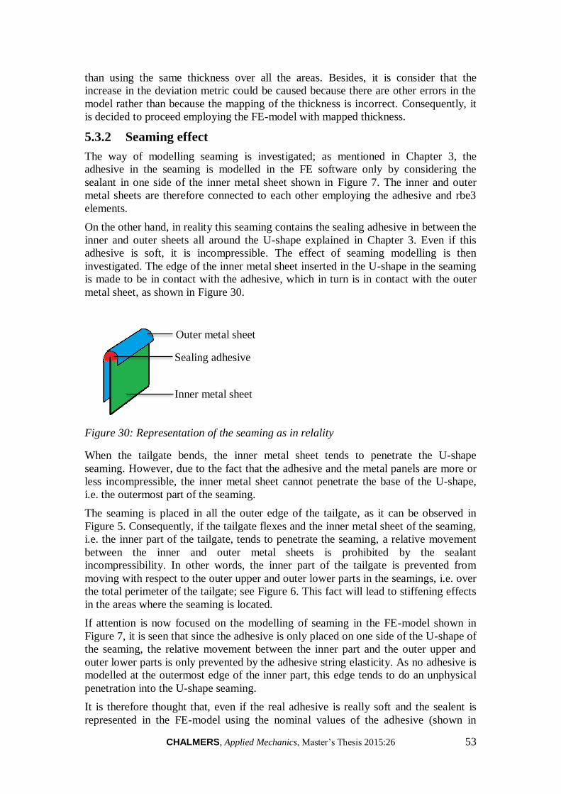
CHALMERS, Applied Mechanics, Master’s Thesis 2015:26 53
than using the same thickness over all the areas. Besides, it is consider that the
increase in the deviation metric could be caused because there are other errors in the
model rather than because the mapping of the thickness is incorrect. Consequently, it
is decided to proceed employing the FE-model with mapped thickness.
5.3.2 Seaming effect
The way of modelling seaming is investigated; as mentioned in Chapter 3, the
adhesive in the seaming is modelled in the FE software only by considering the
sealant in one side of the inner metal sheet shown in Figure 7. The inner and outer
metal sheets are therefore connected to each other employing the adhesive and rbe3
elements.
On the other hand, in reality this seaming contains the sealing adhesive in between the
inner and outer sheets all around the U-shape explained in Chapter 3. Even if this
adhesive is soft, it is incompressible. The effect of seaming modelling is then
investigated. The edge of the inner metal sheet inserted in the U-shape in the seaming
is made to be in contact with the adhesive, which in turn is in contact with the outer
metal sheet, as shown in Figure 30.
Figure 30: Representation of the seaming as in relality
When the tailgate bends, the inner metal sheet tends to penetrate the U-shape
seaming. However, due to the fact that the adhesive and the metal panels are more or
less incompressible, the inner metal sheet cannot penetrate the base of the U-shape,
i.e. the outermost part of the seaming.
The seaming is placed in all the outer edge of the tailgate, as it can be observed in
Figure 5. Consequently, if the tailgate flexes and the inner metal sheet of the seaming,
i.e. the inner part of the tailgate, tends to penetrate the seaming, a relative movement
between the inner and outer metal sheets is prohibited by the sealant
incompressibility. In other words, the inner part of the tailgate is prevented from
moving with respect to the outer upper and outer lower parts in the seamings, i.e. over
the total perimeter of the tailgate; see Figure 6. This fact will lead to stiffening effects
in the areas where the seaming is located.
If attention is now focused on the modelling of seaming in the FE-model shown in
Figure 7, it is seen that since the adhesive is only placed on one side of the U-shape of
the seaming, the relative movement between the inner part and the outer upper and
outer lower parts is only prevented by the adhesive string elasticity. As no adhesive is
modelled at the outermost edge of the inner part, this edge tends to do an unphysical
penetration into the U-shape seaming.
It is therefore thought that, even if the real adhesive is really soft and the sealent is
represented in the FE-model using the nominal values of the adhesive (shown in
Inner metal sheet
Outer metal sheet
Sealing adhesive

54 CHALMERS, Applied Mechanics, Master’s Thesis 2015:26
Table 1), the adhesive string connection is the only contact preventing the mentioned
effect, and thus has to be stiffer. In other words; as there is no adhesive modelled
preventing the penetration of the inner metal sheet, this connection has to be strong
enough to ensure that the inner part does not penetrate into the outer parts.
In consequence, it is decided to use stiffer properties of the adhesive material. The
considered properties are the stiffness and Poisson’s ratio of the solid elements
representing the adhesive shown in Table 1. These properties are employed because
the explained effect that occurs in the seaming is shearing. The inner part tends to
move relative to the outer parts, i.e. parallel to the outer parts, trying to penetrate the
seaming; thus shear stresses are created in the solid elements representing the
adhesive.
It is then necessary to ensure that these solid elements can take high shear stresses
without volume contraction. High stiffness and Poisson’s ratio close to
incompressibility are therefore considered. The values of the material properties
assigned to the adhesive are varied and the outputs from simulations are evaluated for
each modification. The combination of these parameters in the FE-model that resulted
to match closest with test data is the one in which the stiffness of the adhesive
corresponds to steel and Poisson’s ratio represents the incompressibility condition.
The MAC correlation between test data and FE results according to the mentioned
properties is shown in Table 9. The FE-model used includes the mapping of thickness
after metal forming simulations.
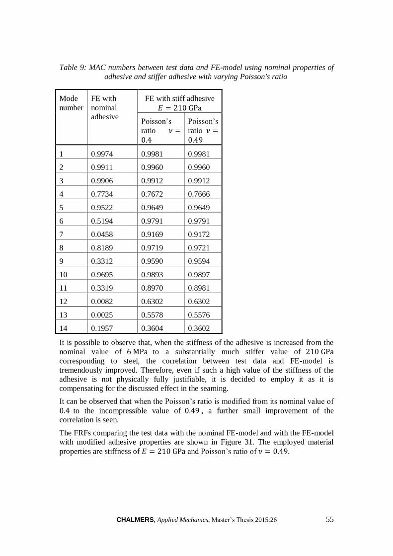
CHALMERS, Applied Mechanics, Master’s Thesis 2015:26 55
Table 9: MAC numbers between test data and FE-model using nominal properties of
adhesive and stiffer adhesive with varying Poisson's ratio
Mode
number
FE with
nominal
adhesive
FE with stiff adhesive
𝐸 = 210 GPa
Poisson’s
ratio 𝜈 =0.4
Poisson’s
ratio 𝜈 =0.49
1 0.9974 0.9981 0.9981
2 0.9911 0.9960 0.9960
3 0.9906 0.9912 0.9912
4 0.7734 0.7672 0.7666
5 0.9522 0.9649 0.9649
6 0.5194 0.9791 0.9791
7 0.0458 0.9169 0.9172
8 0.8189 0.9719 0.9721
9 0.3312 0.9590 0.9594
10 0.9695 0.9893 0.9897
11 0.3319 0.8970 0.8981
12 0.0082 0.6302 0.6302
13 0.0025 0.5578 0.5576
14 0.1957 0.3604 0.3602
It is possible to observe that, when the stiffness of the adhesive is increased from the
nominal value of 6 MPa to a substantially much stiffer value of 210 GPa
corresponding to steel, the correlation between test data and FE-model is
tremendously improved. Therefore, even if such a high value of the stiffness of the
adhesive is not physically fully justifiable, it is decided to employ it as it is
compensating for the discussed effect in the seaming.
It can be observed that when the Poisson’s ratio is modified from its nominal value of
0.4 to the incompressible value of 0.49 , a further small improvement of the
correlation is seen.
The FRFs comparing the test data with the nominal FE-model and with the FE-model
with modified adhesive properties are shown in Figure 31. The employed material
properties are stiffness of 𝐸 = 210 GPa and Poisson’s ratio of 𝜈 = 0.49.

56 CHALMERS, Applied Mechanics, Master’s Thesis 2015:26
Figure 31: Comparison of FRFs of test data and FE-model using nominal and
modified adhesive properties
It is seen that when the modified properties of the solid elements representing the
adhesive in the FE-model are utilised, the FRFs extracted from the FE software result
to substantially improve the curve fit with the test data.
The deviation metric between test data and FE-model is shown in Table 10. The
metric is calculated with the FE-model before and after the mentioned modifications
on the seam stiffness and Poisson’s ratio are performed in the frequency range 10 −195 Hz.
Table 10: Deviation metric between state-space model of test data and FE-model
before and after changing the parameters in the adhesive
Variable FE-model with
nominal adhesive
prop. [−]
FE-model with
modified adhesive
prop. [−]
Improvement
[%]
Deviation metric 2.428 1.321 45.6
According to the deviation metric, the FE-model with the modified properties of the
solid elements representing the adhesive is a much closer representation of reality.
The metric almost halves with respect to the model where only the thickness is
mapped.
An additional investigation revealed that the adhesive string crossing the middle of
the tailgate shown in Figure 6 is not affecting the results, i.e. if the nominal value of
the adhesive is employed in this string instead of the calculated stiffer one, the FRFs
are not influenced. It is then concluded that the stiffness of this string is not
identifiable from the measured test data. This proves that the improvement of the FE-
model when utilising stiffer adhesive is accounting for the seaming effect and not the
gluing itself, as no seaming is done in this middle glued joint of the model.
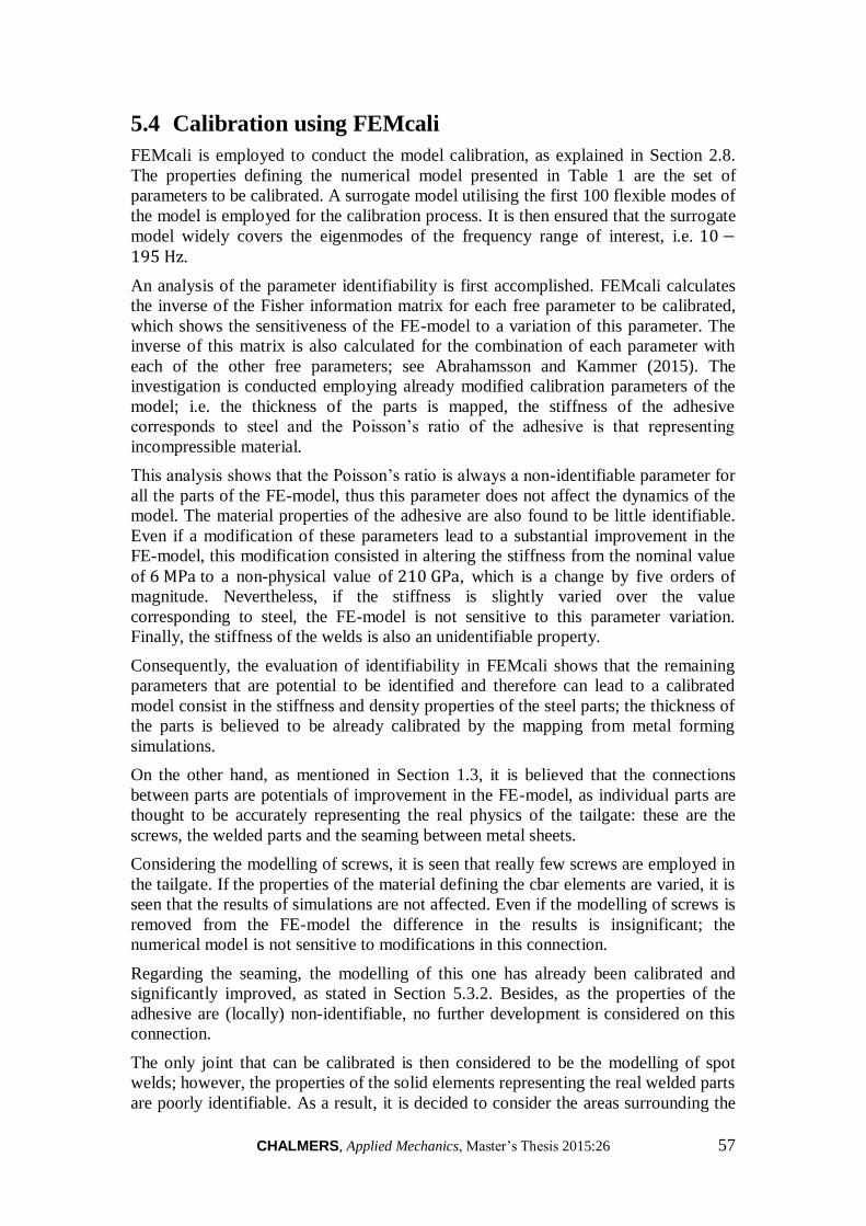
CHALMERS, Applied Mechanics, Master’s Thesis 2015:26 57
5.4 Calibration using FEMcali
FEMcali is employed to conduct the model calibration, as explained in Section 2.8.
The properties defining the numerical model presented in Table 1 are the set of
parameters to be calibrated. A surrogate model utilising the first 100 flexible modes of
the model is employed for the calibration process. It is then ensured that the surrogate
model widely covers the eigenmodes of the frequency range of interest, i.e. 10 −195 Hz.
An analysis of the parameter identifiability is first accomplished. FEMcali calculates
the inverse of the Fisher information matrix for each free parameter to be calibrated,
which shows the sensitiveness of the FE-model to a variation of this parameter. The
inverse of this matrix is also calculated for the combination of each parameter with
each of the other free parameters; see Abrahamsson and Kammer (2015). The
investigation is conducted employing already modified calibration parameters of the
model; i.e. the thickness of the parts is mapped, the stiffness of the adhesive
corresponds to steel and the Poisson’s ratio of the adhesive is that representing
incompressible material.
This analysis shows that the Poisson’s ratio is always a non-identifiable parameter for
all the parts of the FE-model, thus this parameter does not affect the dynamics of the
model. The material properties of the adhesive are also found to be little identifiable.
Even if a modification of these parameters lead to a substantial improvement in the
FE-model, this modification consisted in altering the stiffness from the nominal value
of 6 MPa to a non-physical value of 210 GPa, which is a change by five orders of
magnitude. Nevertheless, if the stiffness is slightly varied over the value
corresponding to steel, the FE-model is not sensitive to this parameter variation.
Finally, the stiffness of the welds is also an unidentifiable property.
Consequently, the evaluation of identifiability in FEMcali shows that the remaining
parameters that are potential to be identified and therefore can lead to a calibrated
model consist in the stiffness and density properties of the steel parts; the thickness of
the parts is believed to be already calibrated by the mapping from metal forming
simulations.
On the other hand, as mentioned in Section 1.3, it is believed that the connections
between parts are potentials of improvement in the FE-model, as individual parts are
thought to be accurately representing the real physics of the tailgate: these are the
screws, the welded parts and the seaming between metal sheets.
Considering the modelling of screws, it is seen that really few screws are employed in
the tailgate. If the properties of the material defining the cbar elements are varied, it is
seen that the results of simulations are not affected. Even if the modelling of screws is
removed from the FE-model the difference in the results is insignificant; the
numerical model is not sensitive to modifications in this connection.
Regarding the seaming, the modelling of this one has already been calibrated and
significantly improved, as stated in Section 5.3.2. Besides, as the properties of the
adhesive are (locally) non-identifiable, no further development is considered on this
connection.
The only joint that can be calibrated is then considered to be the modelling of spot
welds; however, the properties of the solid elements representing the real welded parts
are poorly identifiable. As a result, it is decided to consider the areas surrounding the
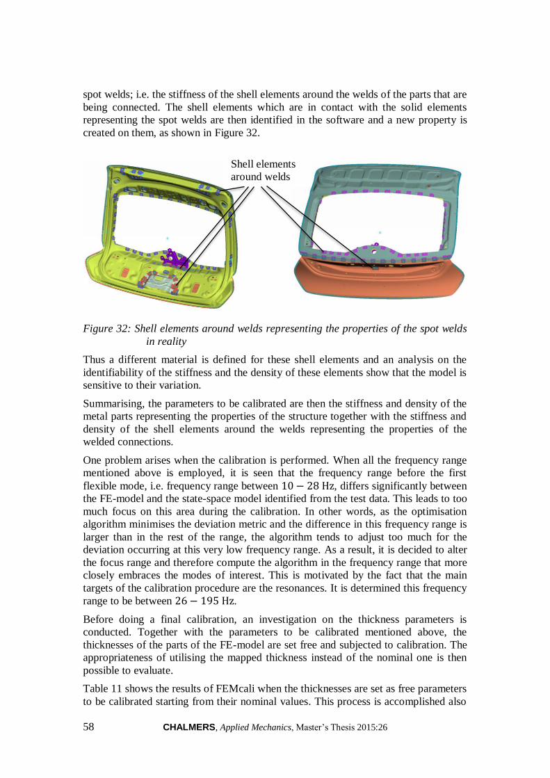
58 CHALMERS, Applied Mechanics, Master’s Thesis 2015:26
spot welds; i.e. the stiffness of the shell elements around the welds of the parts that are
being connected. The shell elements which are in contact with the solid elements
representing the spot welds are then identified in the software and a new property is
created on them, as shown in Figure 32.
Figure 32: Shell elements around welds representing the properties of the spot welds
in reality
Thus a different material is defined for these shell elements and an analysis on the
identifiability of the stiffness and the density of these elements show that the model is
sensitive to their variation.
Summarising, the parameters to be calibrated are then the stiffness and density of the
metal parts representing the properties of the structure together with the stiffness and
density of the shell elements around the welds representing the properties of the
welded connections.
One problem arises when the calibration is performed. When all the frequency range
mentioned above is employed, it is seen that the frequency range before the first
flexible mode, i.e. frequency range between 10 − 28 Hz, differs significantly between
the FE-model and the state-space model identified from the test data. This leads to too
much focus on this area during the calibration. In other words, as the optimisation
algorithm minimises the deviation metric and the difference in this frequency range is
larger than in the rest of the range, the algorithm tends to adjust too much for the
deviation occurring at this very low frequency range. As a result, it is decided to alter
the focus range and therefore compute the algorithm in the frequency range that more
closely embraces the modes of interest. This is motivated by the fact that the main
targets of the calibration procedure are the resonances. It is determined this frequency
range to be between 26 − 195 Hz.
Before doing a final calibration, an investigation on the thickness parameters is
conducted. Together with the parameters to be calibrated mentioned above, the
thicknesses of the parts of the FE-model are set free and subjected to calibration. The
appropriateness of utilising the mapped thickness instead of the nominal one is then
possible to evaluate.
Table 11 shows the results of FEMcali when the thicknesses are set as free parameters
to be calibrated starting from their nominal values. This process is accomplished also
Shell elements
around welds

CHALMERS, Applied Mechanics, Master’s Thesis 2015:26 59
calibrating on the other parameters of the model, so it is ensured that the calibrated
thickness values are not compensating for another source of error. It also shows the
thicknesses of the different parts in the model according to their nominal values.
Finally, the mean value of the thickness at each part of the tailgate according to the
mapped thicknesses is presented in the last column.
Table 11: Comparison of calibrated thickness with nominal and mean of mapped
thickness in the FE-model
Part of the tailgate
Calibrated
thickness [mm] Nominal
thickness [mm] Mean of mapped
thickness [mm]
Inner part 0.641 0.7 0.5901
Outer upper part 0.6481 0.7 0.6546
Outer lower part 0.7129 0.8 0.7485
Wiper motor bracket 1.4399 1.5 1.488
Latch reinforcement 1.4134 1.5 1.466
Upper reinforcements 1.152 1.2 1.1518
Lower reinforcements 1.9535 2 -
One notes that the calibrated thicknesses converge to numbers closer to the mean
value of the mapped thicknesses rather than to the nominal thicknesses of the parts.
Therefore, it is strongly believed that mapping the thicknesses to the FE-model
according to the metal forming simulations is an improvement in the numerical
model. It represents reality more accurately as the deviation metric between test data
and the analytical model is lower.
Furthermore, proceeding with the calibration of the stiffness and density of the
different parts, a reflection on this purpose is conducted. The aim of the calibration is
to find general modelling guidelines that can be employed in similar FE-models in
future applications rather than obtaining an extremely good fitness between the FRFs
of this individual FE-model with respect to test data. In other words, it is desired to
determine findings that are in correspondence to physical representation, thus
parameter values converging to non-physical results in reality are avoided. Apart from
that, the calibrated parameters have to correspond to practical guidelines to be used in
the future; the idea of employing a different parameter for each part is therefore
discarded.
In consequence, it is concluded to employ parameters that encompass the whole
model: two parameters for the metal parts, i.e. stiffness and density, and two
parameters for the shell elements around all the welds, i.e. stiffness and density.
The optimisation algorithm to search for the minimum deviation metric is then
computed. This time, the FE-model is utilised including the mapped thicknesses.
Nevertheless, the results converge to extremely low values for the density of the shell
elements around the welds, which are not physically reasonable. In addition, it is seen
that the curve fit to the test data is only slightly improved when this parameter is
included compared to when only the other three are employed; it is therefore

60 CHALMERS, Applied Mechanics, Master’s Thesis 2015:26
concluded to remove the parameter representing the density of the connection in the
spot welds.
Finally, the process is conducted using only three parameters: the stiffness and density
of all the metal parts and the parameter representing the stiffness of the spot welds,
i.e. stiffness of the shell elements around all the welded points. The results that
converged to the minimum deviation metric are shown in Table 12.
Table 12: Results from calibration on stiffness and density of metal parts
Parameter Nominal value Calibrated value Difference [%]
Stiffness of metal
parts 𝐸 [GPa] 210.0 206.26 1.8
Density of metal
parts 𝜌 [kg
m3]
7850.0 7467.2 5
Stiffness of shell
elements around
welds 𝐸 [MPa] 210.0 200.11 4.8
Deviation metric Nominal FE Calibrated FE Improvement [%]
1.321 1.146 13.8
As it is possible to observe, all the values tend to decrease from their nominal values.
The stiffness of the metal parts decreases 2%, while the density of the metal parts and
the parameter representing the stiffness in welds reduces by 5%.
The numerical model is improved when the calibrated values are employed with
respect to fitting to the FRFs of the identified state-space model. The deviation metric
for the calibrated FE-model is reduced to 86.8% of the deviation for the FE-model
employed at the start of calibration. It is necessary to consider that this starting set of
parameters does not correspond to the nominal model; it contains the mapped
thicknesses of the parts and the properties of the adhesive have been modified.
The FRFs showing the FE-model before and after the calibration can be seen in
Figure 33. The FE-model is compared with the raw test data measured on tailgata A,
i.e. data with which the calibration process in FEMcali is performed. The FRFs are
shown in the frequency range lower than 200 Hz . Higher frequencies are not
employed for the calibration process, as mentioned above.
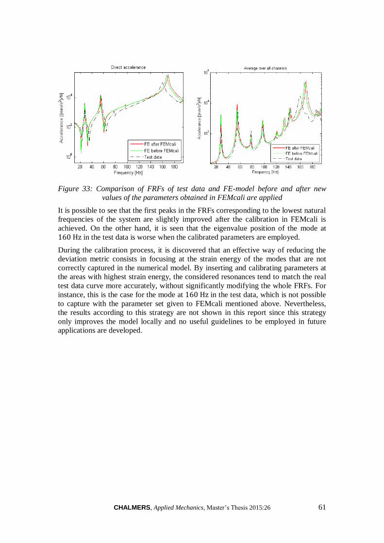
CHALMERS, Applied Mechanics, Master’s Thesis 2015:26 61
Figure 33: Comparison of FRFs of test data and FE-model before and after new
values of the parameters obtained in FEMcali are applied
It is possible to see that the first peaks in the FRFs corresponding to the lowest natural
frequencies of the system are slightly improved after the calibration in FEMcali is
achieved. On the other hand, it is seen that the eigenvalue position of the mode at
160 Hz in the test data is worse when the calibrated parameters are employed.
During the calibration process, it is discovered that an effective way of reducing the
deviation metric consists in focusing at the strain energy of the modes that are not
correctly captured in the numerical model. By inserting and calibrating parameters at
the areas with highest strain energy, the considered resonances tend to match the real
test data curve more accurately, without significantly modifying the whole FRFs. For
instance, this is the case for the mode at 160 Hz in the test data, which is not possible
to capture with the parameter set given to FEMcali mentioned above. Nevertheless,
the results according to this strategy are not shown in this report since this strategy
only improves the model locally and no useful guidelines to be employed in future
applications are developed.

62 CHALMERS, Applied Mechanics, Master’s Thesis 2015:26
6 Results and Discussion
The results obtained after the whole calibration process is summarized and the
calibrated FE-model is presented and compared to the nominal model. It is necessary
to take into account that the numerical model has been calibrated against one of the
measured objects, i.e. tailgate A. The results are therefore compared to test data
corresponding to this object. Moreover, the calibration has been accomplished
employing the frequency range between 26 − 195 Hz.
6.1 Nominal vs calibrated FE-model
First of all, the mass of the numerical model is evaluated and compared to the mass of
the real measured objects both before and after calibration. The weight of the
components is shown in Table 13.
Table 13: Comparison of mass of nominal and calibrated FE-model with test objects
Object Parameter Value
3 physical
objects
Mean of mass [kg] 10.513
Dispersion [%] 0.14
Nominal
FE-model Mass [kg] 10.82
Difference with test [%] 2.9
Calibrated
FE-model Mass [kg] 9.738
Difference with test [%] 7.6
It is seen that the mass of the tested tailgates is really similar and therefore the
dispersion between the objects is very small; there is only a 0.14% difference
between the three of them.
On the other hand, the mass of the real components differs from the FE-model, both
before and after calibration. The nominal FE-model of the tailgate is almost
3% heavier than the real objects.
Moreover, the calibrated FE-model is lighter than the real tailgates. The weight of the
numerical model is reduced by slightly more than 10% in the calibration process.
Mapping of the thicknesses reduced it considerably, while the output from FEMcali
states that the density of the metal parts has to be decreased by 5% more. As a result,
the mass of the calibrated analytical model is more than 7% off compared to the
tested articles.
According to the analysis of the mass, the FE-model seems to get worse rather than
improved after calibration. However, if an investigation of the eigenfrequencies of the
system is accomplished as shown in Table 14, a very different behaviour is observed.
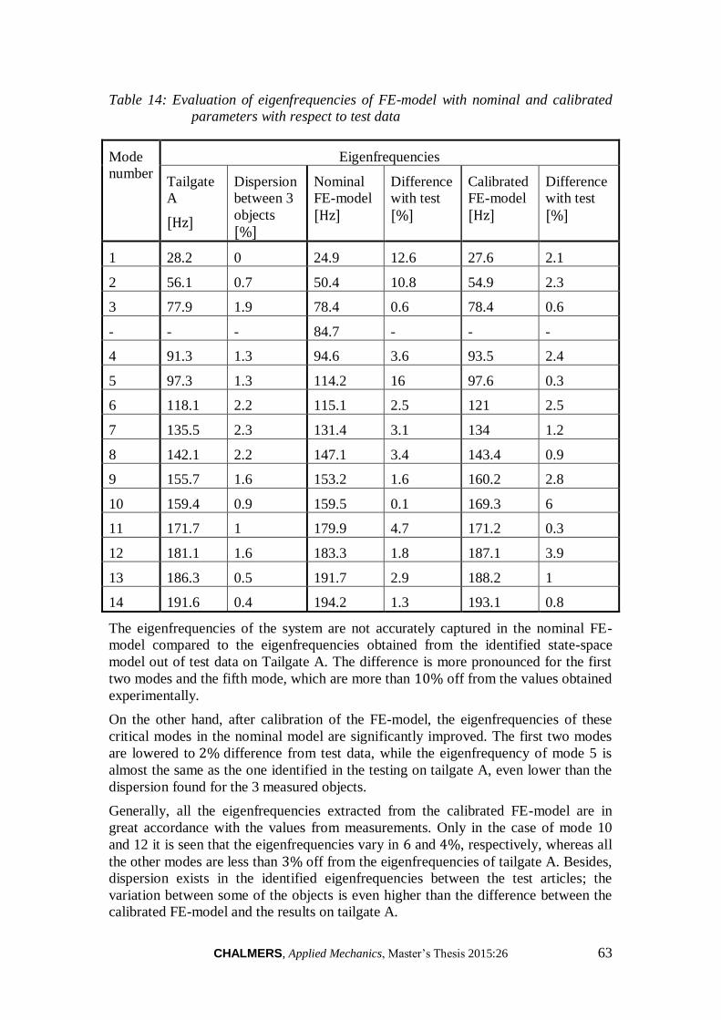
CHALMERS, Applied Mechanics, Master’s Thesis 2015:26 63
Table 14: Evaluation of eigenfrequencies of FE-model with nominal and calibrated
parameters with respect to test data
Mode
number
Eigenfrequencies
Tailgate
A
[Hz]
Dispersion
between 3
objects
[%]
Nominal
FE-model [Hz]
Difference
with test
[%]
Calibrated
FE-model [Hz]
Difference
with test
[%]
1 28.2 0 24.9 12.6 27.6 2.1
2 56.1 0.7 50.4 10.8 54.9 2.3
3 77.9 1.9 78.4 0.6 78.4 0.6
- - - 84.7 - - -
4 91.3 1.3 94.6 3.6 93.5 2.4
5 97.3 1.3 114.2 16 97.6 0.3
6 118.1 2.2 115.1 2.5 121 2.5
7 135.5 2.3 131.4 3.1 134 1.2
8 142.1 2.2 147.1 3.4 143.4 0.9
9 155.7 1.6 153.2 1.6 160.2 2.8
10 159.4 0.9 159.5 0.1 169.3 6
11 171.7 1 179.9 4.7 171.2 0.3
12 181.1 1.6 183.3 1.8 187.1 3.9
13 186.3 0.5 191.7 2.9 188.2 1
14 191.6 0.4 194.2 1.3 193.1 0.8
The eigenfrequencies of the system are not accurately captured in the nominal FE-
model compared to the eigenfrequencies obtained from the identified state-space
model out of test data on Tailgate A. The difference is more pronounced for the first
two modes and the fifth mode, which are more than 10% off from the values obtained
experimentally.
On the other hand, after calibration of the FE-model, the eigenfrequencies of these
critical modes in the nominal model are significantly improved. The first two modes
are lowered to 2% difference from test data, while the eigenfrequency of mode 5 is
almost the same as the one identified in the testing on tailgate A, even lower than the
dispersion found for the 3 measured objects.
Generally, all the eigenfrequencies extracted from the calibrated FE-model are in
great accordance with the values from measurements. Only in the case of mode 10
and 12 it is seen that the eigenfrequencies vary in 6 and 4%, respectively, whereas all
the other modes are less than 3% off from the eigenfrequencies of tailgate A. Besides,
dispersion exists in the identified eigenfrequencies between the test articles; the
variation between some of the objects is even higher than the difference between the
calibrated FE-model and the results on tailgate A.

64 CHALMERS, Applied Mechanics, Master’s Thesis 2015:26
Consequently, it is determined that the calibrated FE-model significantly improves the
capacity of prediction of the eigenfrequencies of the system and gives really good
correlation with the eigenfrequencies identified in the measured data. Finally, it is
seen that in the investigated frequency range mentioned above, the calibrated FE-
model does not predict a mode in an eigenfrequency where the nominal FE-model
does. As a result, according to the calibrated FE-model as well as the test data 14
modes are located in the frequency range of interest, while the nominal numerical
model captures 15 modes.
The same behaviour can be observed if the investigation is performed between the
MAC indices of the FE-model with the test data, as shown in Figure 34.
Figure 34: MAC indices between FE-model and test data. Left: nominal model. Right:
calibrated model.
It is important to note that both in case of the eigenfrequencies and the MAC indices
the spurious modes have been removed.
One observes in the left side of Figure 34 that the nominal FE-model does not
correlate well with the measured data. Only the first flexible modes of the system
have highly correlated eigenvectors, i.e. the nominal model and tailgate A measured
in the experiments have the same dynamic characteristics only at those resonances.
On the other hand, if attention is focused on MAC indices comparing the eigenvectors
of the calibrated FE-model with the eigenvectors of the state-space model identified
from test data on tailgate A, it is seen that the correlation has been substantially
improved. Almost all the resonances in the investigated frequency range have a MAC
index close to one: 8 out of 14 modes are closely correlated, whereas only the last 3
modes in the investigated frequency range are poorly correlated.
In case of mode 4, as previously mentioned, the MAC correlation not being high is
expected due to test conditions rather than because the FE-model is not representative
for this mode.
Additionally, the FRFs extracted from the nominal and calibrated FE-model are
compared to the FRFs obtained in the measurements on tailgate A and presented in
Figure 35.
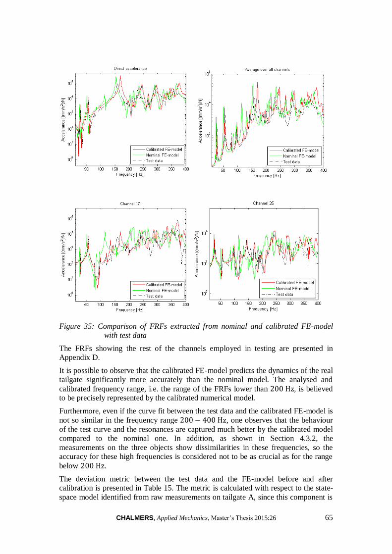
CHALMERS, Applied Mechanics, Master’s Thesis 2015:26 65
Figure 35: Comparison of FRFs extracted from nominal and calibrated FE-model
with test data
The FRFs showing the rest of the channels employed in testing are presented in
Appendix D.
It is possible to observe that the calibrated FE-model predicts the dynamics of the real
tailgate significantly more accurately than the nominal model. The analysed and
calibrated frequency range, i.e. the range of the FRFs lower than 200 Hz, is believed
to be precisely represented by the calibrated numerical model.
Furthermore, even if the curve fit between the test data and the calibrated FE-model is
not so similar in the frequency range 200 − 400 Hz, one observes that the behaviour
of the test curve and the resonances are captured much better by the calibrated model
compared to the nominal one. In addition, as shown in Section 4.3.2, the
measurements on the three objects show dissimilarities in these frequencies, so the
accuracy for these high frequencies is considered not to be as crucial as for the range
below 200 Hz.
The deviation metric between the test data and the FE-model before and after
calibration is presented in Table 15. The metric is calculated with respect to the state-
space model identified from raw measurements on tailgate A, since this component is
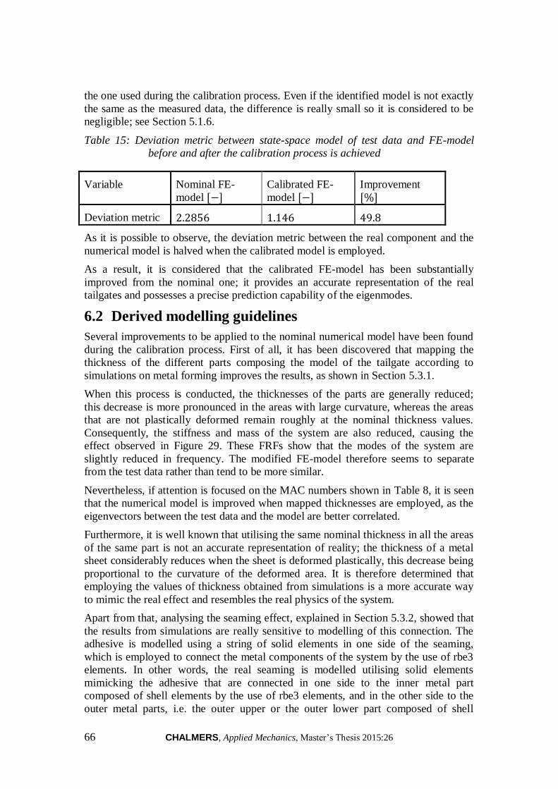
66 CHALMERS, Applied Mechanics, Master’s Thesis 2015:26
the one used during the calibration process. Even if the identified model is not exactly
the same as the measured data, the difference is really small so it is considered to be
negligible; see Section 5.1.6.
Table 15: Deviation metric between state-space model of test data and FE-model
before and after the calibration process is achieved
Variable Nominal FE-
model [−] Calibrated FE-
model [−] Improvement
[%]
Deviation metric 2.2856 1.146 49.8
As it is possible to observe, the deviation metric between the real component and the
numerical model is halved when the calibrated model is employed.
As a result, it is considered that the calibrated FE-model has been substantially
improved from the nominal one; it provides an accurate representation of the real
tailgates and possesses a precise prediction capability of the eigenmodes.
6.2 Derived modelling guidelines
Several improvements to be applied to the nominal numerical model have been found
during the calibration process. First of all, it has been discovered that mapping the
thickness of the different parts composing the model of the tailgate according to
simulations on metal forming improves the results, as shown in Section 5.3.1.
When this process is conducted, the thicknesses of the parts are generally reduced;
this decrease is more pronounced in the areas with large curvature, whereas the areas
that are not plastically deformed remain roughly at the nominal thickness values.
Consequently, the stiffness and mass of the system are also reduced, causing the
effect observed in Figure 29. These FRFs show that the modes of the system are
slightly reduced in frequency. The modified FE-model therefore seems to separate
from the test data rather than tend to be more similar.
Nevertheless, if attention is focused on the MAC numbers shown in Table 8, it is seen
that the numerical model is improved when mapped thicknesses are employed, as the
eigenvectors between the test data and the model are better correlated.
Furthermore, it is well known that utilising the same nominal thickness in all the areas
of the same part is not an accurate representation of reality; the thickness of a metal
sheet considerably reduces when the sheet is deformed plastically, this decrease being
proportional to the curvature of the deformed area. It is therefore determined that
employing the values of thickness obtained from simulations is a more accurate way
to mimic the real effect and resembles the real physics of the system.
Apart from that, analysing the seaming effect, explained in Section 5.3.2, showed that
the results from simulations are really sensitive to modelling of this connection. The
adhesive is modelled using a string of solid elements in one side of the seaming,
which is employed to connect the metal components of the system by the use of rbe3
elements. In other words, the real seaming is modelled utilising solid elements
mimicking the adhesive that are connected in one side to the inner metal part
composed of shell elements by the use of rbe3 elements, and in the other side to the
outer metal parts, i.e. the outer upper or the outer lower part composed of shell
CHALMERS, Applied Mechanics, Master’s Thesis 2015:26 67
elements, utilising rbe3 elements as well. The findings showed that, even if the real
adhesive is really soft, if the stiffness of the solid elements is modified to 210 GPa the
results from the FE-model are substantially improved. Although having the stiffness
of the solid elements corresponding to steel is not physically correct, this value of the
stiffness is compensating for the modelling error due to the effect that the seaming
causes in reality, as explained in Section 5.3.2. The inner metal sheet is in contact
with the adhesive, and the adhesive is in turn in contact with the outer metal sheet. As
these three components are incompressible, the relative movement of the inner sheet
with respect to the outer sheet is prevented by the seam. A modification in the
Poisson’s ratio from the nominal value of 0.4 to the incompressible condition of 0.49
also revealed small improvements in the prediction capability of the numerical model.
The modified properties of the solid elements mimicking the adhesive in the FE-
model are accounting for this behaviour. When the tailgate is bended, the inner metal
sheet in the seaming tends to move relative to the outer metal sheet. As the only
connection between these metals in the seaming occurs through the adhesive, this
connection has to be really stiff to avoid such motion from happening. Hence, even if
the properties of the solid elements do not resemble the real adhesive, it is obvious
that employing these values lead to a more accurate representation of the real physics:
the dynamics of the system are much better predicted in the numerical model.
Moreover, it is believed that the modelling of the seams need to be reconsidered in
order for it representing the real behaviour. The current strategy is too simple and
employing the modified properties has shown that the prediction capability of the
model is substantially in better accordance with reality.
Nevertheless, even if this means complicating the modelling technique, it is suggested
to model the solid elements around the U-shape of the seaming mentioned in Section
5.3.2 and shown in Figure 30. Thus the adhesive in the FE-model mimics the area at
which the inner and outer metal sheets in the seaming are in contact to the adhesive in
real life. If this is accomplished, the results may resemble the reality even better.
Finally, the results when the deviation metric minimisation algorithm was conducted
in FEMcali show that some of the properties in the FE-model should be modified. If
the stiffness and the density of all the metal parts in the analytical model are lowered
2% and 5%, respectively, and at the same time the stiffness of the shell elements
around the welds are decreased in 5%, the deviation metric between the simulations
and the test data is improved in almost 15%. It is therefore advisable to perform this
modification.
It is important to understand that the increase in FE-model prediction accuracy is
caused by the combination of all the calibrated parameters rather than only employing
one modification. In other words, mapping of the thickness has shown to improve the
results and is therefore recommended. In the case of changing the values of the solid
elements modelling the adhesive of seams, it is also strongly believe that this
modification will lead to a more accurate FE-model.
On the other hand, the findings in FEMcali, i.e. correcting the stiffness and density of
the metal parts and the stiffness of the shell elements around the welded areas, have
been found to improve the model only if previously the mapping of the thickness is
accomplished and the altering of the seam properties is conducted. Consequently, if
these two modifications are not performed, it is not possible to conclude whether the
FE-model will improve or not when the properties are changed according to FEMcali.
68 CHALMERS, Applied Mechanics, Master’s Thesis 2015:26
7 Conclusions
Model calibration is based on data obtained from vibration testing; it is therefore
extremely crucial to conduct the experiments with great accuracy and care, as the
success of the calibration cannot be achieved if the measurements are not precise or
contain errors.
With present calibration methods it is necessary to ensure that the measured response
is linear. Hence, the objects have to be measured employing as low amplitude of
excitation as possible in order to avoid rattling effects that lead to non-linear
behaviour of the response.
However, if the system is excited utilising a signal that is too low, noise will most
likely be captured by the accelerometers, destroying test data. As a result, the
amplitude of excitation has to be adjusted to ensure a linear response of the system
that is not buried in noise.
During the measurements, it is discovered that non-linear response due to rattling of
the system sometimes occurs at high frequencies, while the excitation amplitude has
to be higher in low frequencies to capture the response correctly and avoid noise
affecting the results. It is therefore concluded that in vibration testing the amplitude of
excitation should be relatively strong in low frequencies, whereas the magnitude of
the excitation has to be decreased as the frequency increases.
It is determined that a proper sampling strategy for the discrete frequencies employed
in the measurements to evaluate the frequency response functions optimises the
vibration testing in terms of time and required information about the model. As the
half-band width of a damped structural resonance increases linearly with respect to
the frequency at which the mode occurs, the best sampling strategy consists in
employing frequency steps that increase linearly with frequency, thus the number of
frequency samples at each resonance will be approximately constant during the
measured frequency range.
Three different tailgates are measured in this work with the aim of evaluating the
dispersion in the response between the objects. In order for the observed dispersion
only to be influenced by differences in the manufacturing process, the measurements
on the three tailgates have to be performed under exactly the same conditions. The
dispersion due to varying testing conditions can be minimised by using the same
profile and magnitude of excitation for all the objects. Moreover, a great deal of care
has to be taken when doing the set-up of the different objects, thus all the articles are
carefully tested under the same conditions, i.e. the same accelerometer locations, the
same shaker position and direction, the same stinger length, the same external
instruments added, etc.
When doing the set-up of the experiments, it is concluded that employing bungee
cords lead to the response being slightly influenced by the natural frequencies of the
bungee cords. In order to avoid this, the use of ultra-light weight and ultra-strong
fishing lines is suggested. If bungee cords are employed at the top of the set-up and
this are connected to fishing lines, which in turn are connected to the structure to be
tested, the results of the measurements are expected to be of better quality. The
influence from the dynamics of the supporting structure will be minimal and the rigid
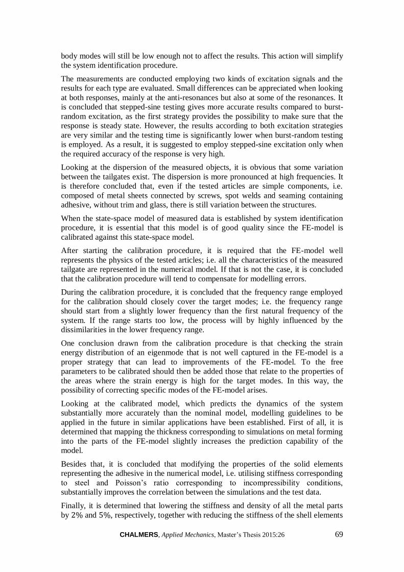
CHALMERS, Applied Mechanics, Master’s Thesis 2015:26 69
body modes will still be low enough not to affect the results. This action will simplify
the system identification procedure.
The measurements are conducted employing two kinds of excitation signals and the
results for each type are evaluated. Small differences can be appreciated when looking
at both responses, mainly at the anti-resonances but also at some of the resonances. It
is concluded that stepped-sine testing gives more accurate results compared to burst-
random excitation, as the first strategy provides the possibility to make sure that the
response is steady state. However, the results according to both excitation strategies
are very similar and the testing time is significantly lower when burst-random testing
is employed. As a result, it is suggested to employ stepped-sine excitation only when
the required accuracy of the response is very high.
Looking at the dispersion of the measured objects, it is obvious that some variation
between the tailgates exist. The dispersion is more pronounced at high frequencies. It
is therefore concluded that, even if the tested articles are simple components, i.e.
composed of metal sheets connected by screws, spot welds and seaming containing
adhesive, without trim and glass, there is still variation between the structures.
When the state-space model of measured data is established by system identification
procedure, it is essential that this model is of good quality since the FE-model is
calibrated against this state-space model.
After starting the calibration procedure, it is required that the FE-model well
represents the physics of the tested articles; i.e. all the characteristics of the measured
tailgate are represented in the numerical model. If that is not the case, it is concluded
that the calibration procedure will tend to compensate for modelling errors.
During the calibration procedure, it is concluded that the frequency range employed
for the calibration should closely cover the target modes; i.e. the frequency range
should start from a slightly lower frequency than the first natural frequency of the
system. If the range starts too low, the process will by highly influenced by the
dissimilarities in the lower frequency range.
One conclusion drawn from the calibration procedure is that checking the strain
energy distribution of an eigenmode that is not well captured in the FE-model is a
proper strategy that can lead to improvements of the FE-model. To the free
parameters to be calibrated should then be added those that relate to the properties of
the areas where the strain energy is high for the target modes. In this way, the
possibility of correcting specific modes of the FE-model arises.
Looking at the calibrated model, which predicts the dynamics of the system
substantially more accurately than the nominal model, modelling guidelines to be
applied in the future in similar applications have been established. First of all, it is
determined that mapping the thickness corresponding to simulations on metal forming
into the parts of the FE-model slightly increases the prediction capability of the
model.
Besides that, it is concluded that modifying the properties of the solid elements
representing the adhesive in the numerical model, i.e. utilising stiffness corresponding
to steel and Poisson’s ratio corresponding to incompressibility conditions,
substantially improves the correlation between the simulations and the test data.
Finally, it is determined that lowering the stiffness and density of all the metal parts
by 2% and 5%, respectively, together with reducing the stiffness of the shell elements

70 CHALMERS, Applied Mechanics, Master’s Thesis 2015:26
around the welded parts by 5% decreases the deviation metric between the numerical
model and the model identified from test data, i.e. improves the fit to test data.
In conclusion, the model is improved both in terms of the individual metal parts
composing the tailgate and in terms of the connections between these parts. While the
mapping of the thickness and the modification of the stiffness and density of the metal
parts is an improvement of the structural behaviour of the system, the correction of
the adhesive to account for the seaming effect and the adjustment of the stiffness in
the shell elements around the spot welds improves the connection of the different
parts of the model.

CHALMERS, Applied Mechanics, Master’s Thesis 2015:26 71
8 Future Work
Further work on the calibration of the FE-model of the tailgate is suggested. FEMcali
has been employed to calibrate the parameters in the FE-model and with the current
set of parameters the deviation metric cannot be further lowered, i.e. the model cannot
be improved.
However, several modifications in the modelling of the parts and connections can be
performed, which will lead to new parameter settings to be calibrated with FEMcali.
One of the parts that is suggested to be further investigated and developed is the
modelling of the seaming. The current modelling strategy is very simplistic and does
not result in a good representation of reality. Hence, it is suggested to model the solid
elements representing the real adhesive all around the U-shape of the seaming even if
this requires more skilful modelling knowledge. In this way, the seaming would be
more accurately represented in the FE-model, and probably the seaming effect
mentioned in the report would also be better captured in the model. Thus defining the
properties of the solid elements with no clear physical connection would not be
necessary.
Besides, parameters in the FE-model that were not considered in this thesis consisted
in parameters of the rbe2 and rbe3 elements. They were not considered because these
are not real parameters, as they cannot be varied from the input file as continuous
variables. The only thing that can be modified is the radius associated to these
elements, i.e. how much the shell elements around the connection contribute to this
connection. This radius defining the influence on the shell elements can only be
modified in the FE software Ansa.
Nevertheless, if a script is developed that enters Ansa and varies the radius of the rbe2
and rbe3 elements automatically, it would be possible to use this parameter as a free
parameter to be calibrated in FEMcali. Therefore, it would be possible to obtain to
which extent the connections defined by these elements are affecting the FE-model.
This can lead to improvements of the modelling of connections.
In this way, it would be possible to calibrate the radius of the rbe2 elements employed
in the modelling of screws using cbar elements together with the radius of the rbe3
elements utilised in the modelling of spot welds and in the modelling of the adhesive,
both corresponding to solid elements.
Finally, it is known that VCC does not have available mapped thickness data from
simulations on metal forming for all the parts of the car. It is therefore suggested to
create a script that automatically captures the curvature of each node and depending
on previously processed data interpolates the value and calculates an approximate
thickness for that node. The mentioned data employed for the interpolation can be
derived by observing the current models with mapped thickness; i.e. by looking at the
thickness at each node and evaluating what has caused the thickness to be reduced
from its nominal value to the current value. Even if the approximation of the thickness
is probably not extremely accurate, it would still be a better representation of reality
than using the same nominal thickness over all the areas of the part, i.e. employ the
same thickness in flat areas as in areas with large curvature.

72 CHALMERS, Applied Mechanics, Master’s Thesis 2015:26
9 References
Abrahamsson, T. (2012). Calibration and validation of structural dynamics models.
Chalmers – Applied Mechanics, Gothenburg.
Abrahamsson T. and Kammer D. (2015). Finite element model calibration using
frequency responses with damping equalization. Mechanical Systems and Signal
Processing, vol. 62-63, pp 218-234.
Allemang, R. J. (2003). The Modal Assurance Criterion – Twenty Years of Use and
Abuse. Sound and Vibration, pp 14-21.
Bachmann, H. et al. (1995). Vibration Problems in Structures. Birkhauser Verlag,
Berlin.
Benson, S. (1997). Press brake technology: a guide to precision sheet metal bending.
Society of Manufacturing Engineers, Dearborn, Michigan, USA, pp. 137-140.
Berbyuk, V. (2014). Structural dynamics control. Chalmers – Applied Mechanics,
Gothenburg. 2nd ed.
BETA CAE Systems S.A. (2014). ANSA v15.1.3 documentation index.
Brüel & Kjær. (1987). Piezoelectric Accelerometers and Vibration Preamplifiers. K.
Larsen & Søn A/S, Glostrup, Denmark.
Craig, R. R. and Kurdila, A. J. (2006). Fundamentals of Structural Dynamics. Wiley,
2nd edition, Hoboken, New Jersey.
Ewins, D. J. (2000). Modal testing: Theory, Practice and Application. Research
Studies Press Ltd, Baldock, England.
Irvine, T. (2000). An introduction to frequency response functions. Retrieved from
publications in vibrationdata.com.
Kammer, D. (1991). Sensor placement for on-orbit modal identification and
correlation of large space structures. Journal of Guidance, Control and Dynamics.
Vol. 14, No. 2, pp. 251-259.
Kammer, D. and Tinker, M. (2004). Optimal placement of triaxial accelerometers for
modal vibration tests.Mechanical Systems and Signal Processing, Vol. 18, No. 1,
pp 29-41.
LMS Test.Lab. The LMS Test.Lab Manual.
Ljung, L. (1987). System Identification: Theory for the user. Prentice Hall,
Englewood Cliffs, USA.
McConnell, K. (1995). Vibration Testing: Theory and Practice. John Wiley & Sons,
New York, USA, pp. 84-91.
McKelvey, T., Akcay H. and Ljung, L. (1996). Subspace-Based Multivariable System
Identification from Frequency Response Data. IEEE Transactions on Automatic
Control, Vol. 41, No.7, pp 960-979.
Moore, B. (1981). Principal component analysis in linear systems: Controllability,
observability, and model reduction. IEEE Transactions on Automatic Control, Vol.
26, No. 1, pp. 17-32.

CHALMERS, Applied Mechanics, Master’s Thesis 2015:26 73
Reynier, M. and Abou-Kandil, H. (1999). Sensors location for updating problems.
Mechanical Systems and Signal Processing, Vol. 13, No. 2, pp. 297-314.
The Modal Shop, Inc. (2015). Frequently Asked Questions: Modal Shakers and
Related Topics. Retrieved 15th of May, 2015 from
http://www.modalshop.com/filelibrary/Modal%20Shaker%20FAQ%20revA.pdf
Van Overschee P. and De Moor B. (1994). N4SID: Subspace Algorithms for the
Identification of Combined Deterministic-Stochastic Systems. Automatica, Vol. 30,
No. 1, pp 75-93.
Van Overschee P. and De Moor B. (1996). Subspace Identification for Linear
Systems, Theory-Implementation-Applications. Kluwer Academic Publishers,
Dordrecht, Netherlands.


CHALMERS, Applied Mechanics, Master’s Thesis 2015:26 i
Appendix A Testing
The point numbering used in the FE-model and to conduct the testing is shown in
Figure A 1.
Figure A 1: Accelerometer numbering for both FE and testing
1
2
3 4 5 6
7
8
9
10
11 13
12 14
15
16
17
19 18
20
21
22 23
24
29
25 26 27 28
30
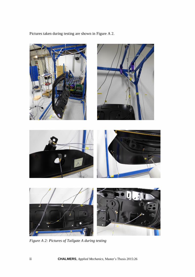
ii CHALMERS, Applied Mechanics, Master’s Thesis 2015:26
Pictures taken during testing are shown in Figure A 2.
Figure A 2: Pictures of Tailgate A during testing
CHALMERS, Applied Mechanics, Master’s Thesis 2015:26 iii
Appendix B Test Results
The dispersion between the test articles for the remaining channels is shown in Figure
B 1.
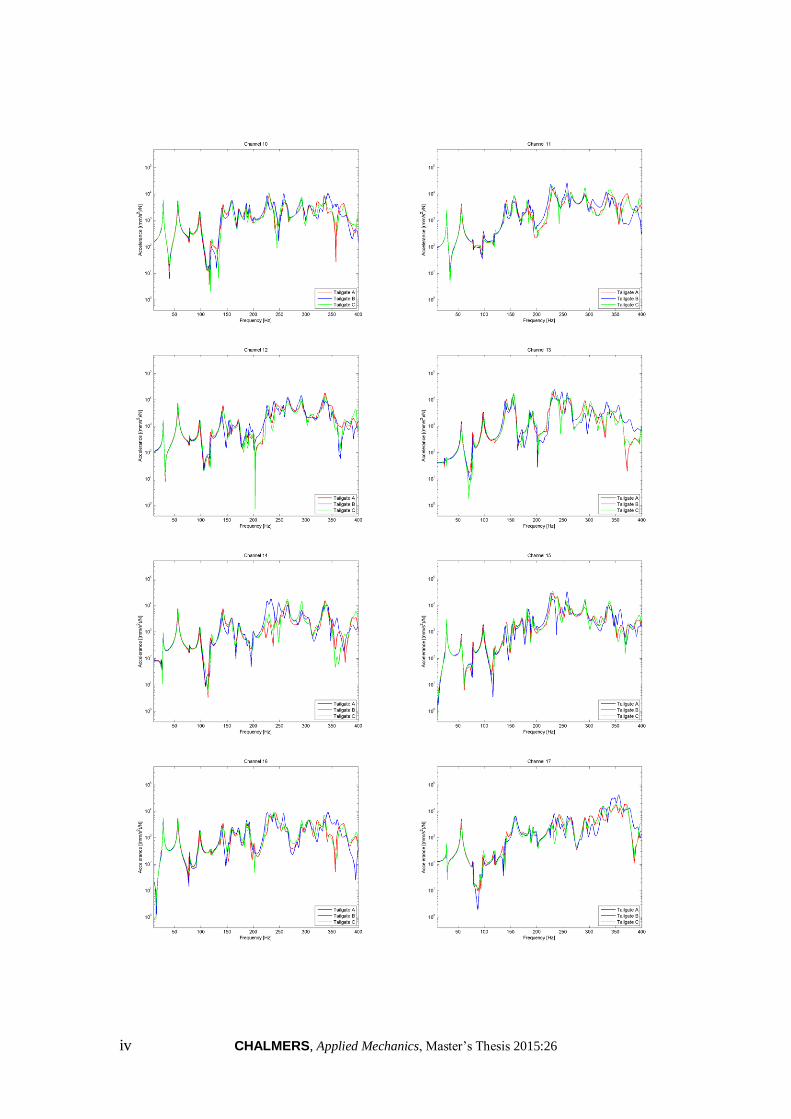
iv CHALMERS, Applied Mechanics, Master’s Thesis 2015:26

CHALMERS, Applied Mechanics, Master’s Thesis 2015:26 v

vi CHALMERS, Applied Mechanics, Master’s Thesis 2015:26
Figure B 1: Dispersion between the 3 tailgates according to stepped-sine excitation
The most significant channels showing differences between measurements performed
employing stepped-sine excitation and burst-random excitation are shown in Figure B
2. The FRFs are represented by the mean of the 3 test objects in order for the
dispersion between the articles to influence the results as little as possible.

CHALMERS, Applied Mechanics, Master’s Thesis 2015:26 vii
Figure B 2: Most significant FRFs showing differences between mean of 3 test
articles measured using two excitation strategies

viii CHALMERS, Applied Mechanics, Master’s Thesis 2015:26
Appendix C Mapped thickness
The metal parts composing the tailgate with mapped thickness according to
simulations of metal forming are shown in Figure C 1.
Figure C 1: Part of the tailgate with mapped thickness from metal forming
simulations (thickness in mm). Upper left: outer upper part, nominal
value 0.7 𝑚𝑚. Upper right: outer lower part, nominal value 0.8 𝑚𝑚.
Middle left: upper reinforcement (the other one is symmetrical),
nominal value 1.2 𝑚𝑚 . Middle right: latch reinforcement, nominal
value 1.5 𝑚𝑚. Lower left: wiper motor bracket, nominal value 1.5 𝑚𝑚.

CHALMERS, Applied Mechanics, Master’s Thesis 2015:26 ix
Appendix D FE-model vs test data
The remaining channels showing the comparison between FRFs extracted from the
FE-model employing the nominal model and the calibrated model with the test data
can be observed in Figure D 1.

x CHALMERS, Applied Mechanics, Master’s Thesis 2015:26
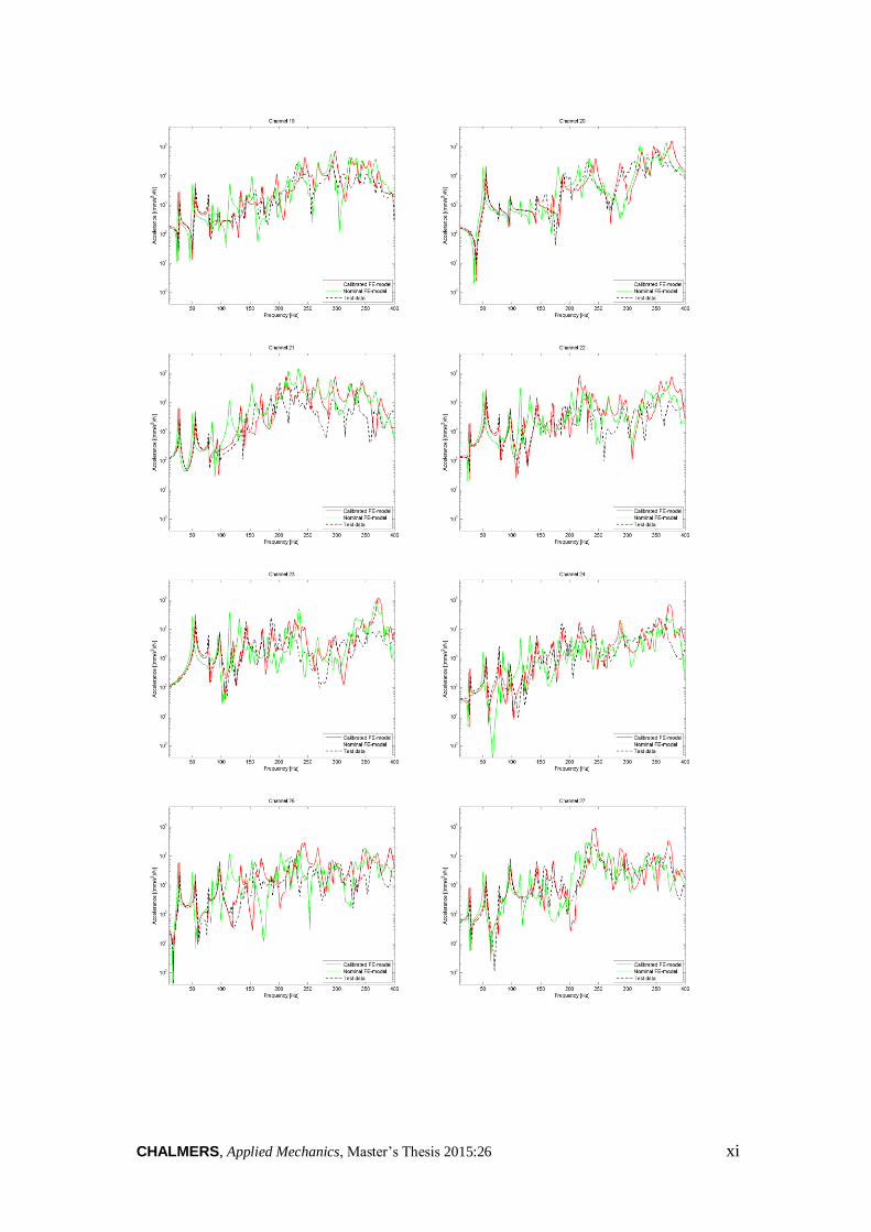
CHALMERS, Applied Mechanics, Master’s Thesis 2015:26 xi
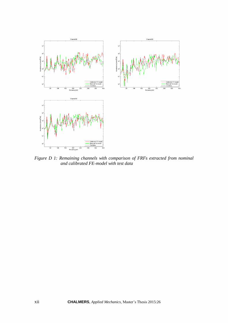
xii CHALMERS, Applied Mechanics, Master’s Thesis 2015:26
Figure D 1: Remaining channels with comparison of FRFs extracted from nominal
and calibrated FE-model with test data