Modal analysis of non-classically damped linear...

EARTHQUAKE ENGINEERING AND STRUCTURAL DYNAMICS, VOL. 14, 217-243 (1986)

MODAL ANALYSIS OF NON-CLASSICALLY DAMPED LINEAR SYSTEMS

ANESTIS S. VELETSOS. A N D CARLOS E. VENTURAS Department of Civil Engineering, Rice University, Houston, Texas 77251, U S A .

SUMMARY A critical, textbook-like review of the generalized modal superposition method of evaluating the dynamic response of non- classically damped linear systems is presented, which it is hoped will increase the attractiveness of the method to structural engineers and its application in structural engineering practice and research. Special attention is given to identifying the physical significance of the various elements of the solution and to simplifying its implementation. It is shown that the displacements of a nonclassically damped n-degree-of-freedom system may be expressed as a linear combination of the displacements and velocities of n similarly excited single-degree-of-freedom systems, and that once the natural frequencies of vibration of the system have been determined, its response to an arbitrary excitation may be computed with only minimal computational effort beyond that required for the analysis of a classically damped system of the same size. The concepts involved are illustrated by a series of exqmples, and comprehensive numerical data for a three-degree-of- freedom system are presented which elucidate the effects of several important parameters. The exact solutions for the system are also compared over a wide range of conditions with those computed approximately considering the system to be classically damped, and the interrelationship of two sets of solutions is discussed.

INTRODUCTION

The modal superposition method is generally recognized as a powerful method for evaluating the dynamic response of viscously damped linear structural systems. The method enables one to express the response of a multi-degree-of-freedom system as a linear combination of its corresponding modal responses. Two versions of the procedure are in use: (1) the time history version, in which the modal responses are evaluated as a function of time and then combined to yield the response history of the system; and (2) the response spectrum version, in which first the maximum values of the modal responses are determined, usually from the response spectrum applicable to the particular excitation and damping under consideration, and the maximum response of the system is then computed by an appropriate combination of the modal maxima.

When damping is of the form specified by Caughey and OKelly,' the natural modes of vibration of the system are real-valued and identical to those of the associated undamped system. Systems satisfying this condition are said to be classically damped, and the modal superposition method for such systems is referred to as the classical modal method.

The classical modal method has found widespread application in civil engineering practice because of its conceptual simplicity, ease of application and the insight it provides into the action of the system. The response spectrum variant of the method, which makes it possible to identify and consider only the dominant terms in the solution, is particularly useful for making rapid estimates of maximum response values.

Viscously damped systems that do not satisfy the Caughey-OKelly condition generally have complex- valued natural modes. Such systems are said to be non-classically damped, and their response may be evaluated by a generalization of the modal superposition method due to Foss.'

Although well e~tablished,'-~ the generalized modal method has found only limited application in structural engineering practice. Several factors appear to have contributed to this: (a) the generalized method is

Brown and Root Professor. t Graduate Student.

0098-8847/86/020217-27$13.50 0 1986 by John Wiley & Sons, Ltd

Received 4 January 1985 Revised 21 June 1985

218 A. S. VELETSOS AND C. E. VENTURA

inherently more involved than the classical; (b) when used in conjunction with the response spectrum concept, it has had to rely on approximations of questionable accuracy; and (c) perhaps most important, the physical meanings of the elements of the solution for this method have not yet been identified as well as those for the classical modal method.

Considering that the specification of the nature and magnitude of damping in structures is subject to considerable uncertainty, the assumption of classical damping may be a justifiable approximation in many practical applications. There are instances, however, in which a more refined analysis is definitely warranted, and it is important that the attractiveness and reliability of the generalized procedure be improved. This paper is intended to be responsive to this need.

Its broad objectives are: (1) to simplify the implementation of the generalized modal method for evaluating the dynamic response of non-classically damped linear structures; and (2) by clarifying the physical significance of the elements of this method, to increase the attractiveness of the method to, and its use by, structural engineers.

The method is described by reference to cantilever structures excited at the base, and it is then applied to force-excited systems. Following an examination of the natural frequencies and modes of vibration of such systems, the free vibrational response is formulated in several alternative forms, and the more convenient form, in combination with the concepts employed in the development of Duhamel's integral for single-degree-of- freedom systems," is used to obtain the solution for forced vibration. Novel features of the present treatment are: the physical interpretation of the solutions represented by complex conjugate pairs of characteristic vectors, the use of these solutions as building blocks in the definition of the free vibrational and forced vibrational responses of the system, the identification of some useful relationships for the vectors in the expression for forced vibration, and the analysis of systems for which some of the natural modes are real- valued and the others are complex.

It is shown that the transient displacements of a non-classically damped multi-degree-of-freedom system may be expressed as a linear combination of the deformations and the true relative velocities of a series of similarly excited single-degree-of-freedom systems, and that the analysis may be implemented with only minor computational effort beyond that required for a classically damped system of the same size. The concepts involved are illustrated by a series of examples, and comprehensive numerical solutions are presented which elucidate the sensitivity of the response to variations in several important parameters. The exact solutions also are compared with those obtained by an approximate modal superposition involving the use of classical modes of vibration," and the interrelationship of the two sets of solutions is discussed.

Although use is made ofcomplex-valued algebra in the derivation of some of the equations presented herein, all final expressions are presented in terms of real-valued quantities.

Notation

summarized in Appendix 11. The symbols used in this paper are defined when first introduced in the text, and those used extensively are

STATEMENT OF PROBLEM

A viscously damped, linear cantilever system with n degrees of freedom is considered. The system is presumed to be excited by a base motion the acceleration of which is xg(t). The response of this system is governed by the equations

(1)

in which {x} is the column vector of the displacements of the nodes relative to the moving base; a dot superscript denotes differentiation with respect to time, t ; { l } is a column vector of ones; and [m], [c] and [k] are the mass matrix, damping matrix and stiffness matrix of the system, respectively. The latter matrices are real and symmetric; additionally, [c] and [k] are positive semi-definite, and [m] is positive definite. The objective is to elucidate the analysis of the response of the system when no further restriction is imposed on the form of the damping matrix.

[ml + [CI 1x1 + [kl I.) = - [m1{1 F&Z)

MODAL ANALYSIS OF NON-CLASSICALLY DAMPED LINEAR SYSTEMS 219

NATURAL FREQUENCIES AND MODES

For a system in free vibration, the right-hand member of equation (1) vanishes, and the equation admits a solution of the form

where r is a characteristic value and { $1 is the associated characteristic vector or natural mode. On substituting equation (2) into the homogeneous form of equation (l), one obtains the characteristic value problem

(3)

{XI = We' ' (2)

(r2[m1 + r [ c l + Ckl) {$I = (01 in which {0} is the null vector.

Rather than through the solution of the system of equations (3), the desired values of r and the associated { $} may be determined more conveniently by first reducing the system of n second order differential equations (1) to a system of 2n first order differential equations, as suggested in References 3 and 4. Summarized briefly in Appendix I, this approach leads to a characteristic value problem of the form

4 4 1 (21 + P I { Z > = (0) (4)

in which [ A ] and [ B ] are symmetric, real matrices of size 2n by 2n; and { Z } is a vector of 2n elements, of which the lower n elements represent the desired modal displacements, {$}, and the upper n elements represent the associated velocities, r { $}. Equation (4) may be solved by well established procedures.

Provided the amount of damping in the system is not very high, the characteristic values occur in complex conjugate pairs with either negative or zero real parts. For a system with n degrees of freedom, there are n pairs of characteristic values, and to each such pair there corresponds a complex conjugate pair of characteristic vectors.

Let rj and Ti be a pair of characteristic values defined by

} = -q jk ip j 'i

and

be the associated pair of characteristic vectors. In these expressions, i = J - 1; qj and pj are real positive scalars; and {dj} and {xi } are real-valued vectors of n elements each. Further, let pi be the modulus of r j , i.e.

Then the characteristic values may be expressed as

and the following relationship between pi and p j is determined from equation (7):

P j=p j J (1 -Cf ) (10)

The values of pi are numbered in ascending order, and the values of rj and the associated vectors, {$j}, are numbered in the order of the corresponding pi .

Equations (9) are the same as those governing the characteristic roots of a viscously damped single-degree- of-freedom (SDF) system with an undamped circular natural frequency pi and a damping factor Ci. Furthermore, equation (10) is the same as that relating the undamped and damped frequencies of such a system (see second section in Appendix I). In the following developments, pi will be referred to as the j th pseudo-


undamped circular natural frequency of the system; pj will be referred to as the corresponding damped frequency; and T j as the j th modal damping factor. It should be noted that p j is a function of the amount of system damping present and, hence, differs from the corresponding frequency of the associated undamped system. Where confusion may arise, the latter frequency will be denoted by the symbol pp.

Reduction for undamped and classically damped systems

valued. Accordingly, { x i } = {O}, { t j j } = Pj} = {$j}, and pi = p j = pi. For an undamped system, the characteristic values r j are purely imaginary and the natural modes are real-

Caughey and OKelly' have shown that if the damping matrix of the system satisfies the identity

0

[ C I [ M I - ' PI = Ckl Cml - ' CCI (11)

the natural modes are real-valued and equal to those of the associated undamped system. The exponent in this expression denotes the inverse of a matrix. The characteristic values in this case appear in complex conjugate pairs, and the modulus of each pair, p j , is the same as the circular natural frequency of the associated undamped system, p y . The Rayleigh form of damping," for which [c ] is proportional to either [m] or [ k ] or is a linear combination of the two, is a special case of equation (1 1).

Orthogonality of modes

conjugate pair of modes, satisfies the following orthogonality relations: Any pair of characteristic vectors corresponding to distinct characteristic values, including a complex

and

The derivation of these expressions is reviewed briefly in the third section of Appendix I.

Appendix I) that

On substituting this equation into equation (12) and making use of the fact that the real and imaginary parts of the resulting expression must be zero, one obtains the well-known relation

For a classically damped system for which { I c l j } = { $ j } and pi = pp, it can be shown (see fourth section of

{ $ j }'CC1 {$k} = 2Tj P j {$j }'[ml { $ k } (14)

{ $ j { $ k } = 0 for r k # rj (15)

{$j )'[kl {$k} = for rk # ' j (16)

Furthermore, on substituting the latter equation into equation (1 3), one obtains

It should be recalled that the quantities p j and {$j } in these expressionsare the same as those for the associated undamped system.

Examples The sensitivity of the free vibrational characteristics of a non-classically damped system to the magnitude

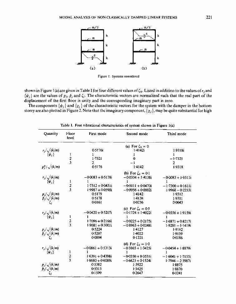
and distribution of the damping present are examined in this section for the three-storey building frame shown in Figure 1. The structure is presumed to be of the shear-beam type with uniform storey stiffnesses, k , and with floor masses m, m and 4 2 , as indicated. System damping is concentrated either in the bottom storey or the top storey. The damping coefficient, c, is expressed in the form

c = To Jh) (1 7) and several different values of the dimensionless constant, lo, are used. The damping matrices for these systems do not satisfy equation (1 1).

The characteristic values and vectors of these systems were evaluated by use of a standard computer program13 making use of the procedure reviewed in the first section of Appendix I. The results for the system

MODAL ANALYSIS OF NON-CLASSICALLY DAMPED LINEAR SYSTEMS 22 1

(a) (b)

Figure I . Systems considered

shown in Figure 1 (a) are given in Table 1 for four different values of T o . Listed in addition to the values of r j and { $ j ) are the values of p i , pi and c j . The characteristic vectors are normalized such that the real part of the displacement of the first floor is unity and the corresponding imaginary part is zero.

The components { 4 j } and { x j } of the characteristic vectors for the system with the damper in the bottom storey are also plotted in Figure 2. Note that the imaginary component, { x j }, may be quite substantial for high

Table I. Free vibrational characteristics of system shown in Figure l(a)

Quantity Floor First mode Second mode Third mode level

1 2 3

1 2 3

1 2 3

1 2 3

05176i 1 1.7321 2 05176

-00083 + 0.51 78i 1 1.7312 +00431i I .9987 + 0.0598i

0.5179 0.5178 0.0161

-00420 + 052073. 1 1.7096+0.2166i 1.9681 +03001i

0.5224 05207 0.0804

-00861 +05313i 1 1.6391 +04398i 1.8680 + 0.60891

0.5382 05313 0.1 599

(a) For To = 0 1.41 42i 1 0

-1 1.4142

(b) For lo = 0 1 -00334+ 1.413%

-00011+00470i -09956 + 0.0002i

1.4142 1.4138 0.0236

(c) For lo = 0 5 -01724+ 14022i

-00225 + 0.21751 -08963 + 002483

1.4127 1.4022 01221

(d) For lo = 1.0 -03865 + 1.3425

-00350 + 03531i -06623 + 01 524i

1.3922 1.3425 02647

1

1

1

1-931 8i 1

2 1.9318

- 1.7321

-00083 + 1.931 li 1

-1.7300+0.1611i 1.9968 -0.22331

1.9312 1.931 1 0.0043

-00356 + 1.91591 1

-1.6871 +@8217i 1.9281 - 1.1419i

1.9162 1.9159 00186

-00454 + 1.88703 1

-16041 + 1.71551 1.7944 - 2.3987i

1 %875 1.8870 0.024 1

222 A. S. VELETSOS A N D C. E. VENTURA

1x11

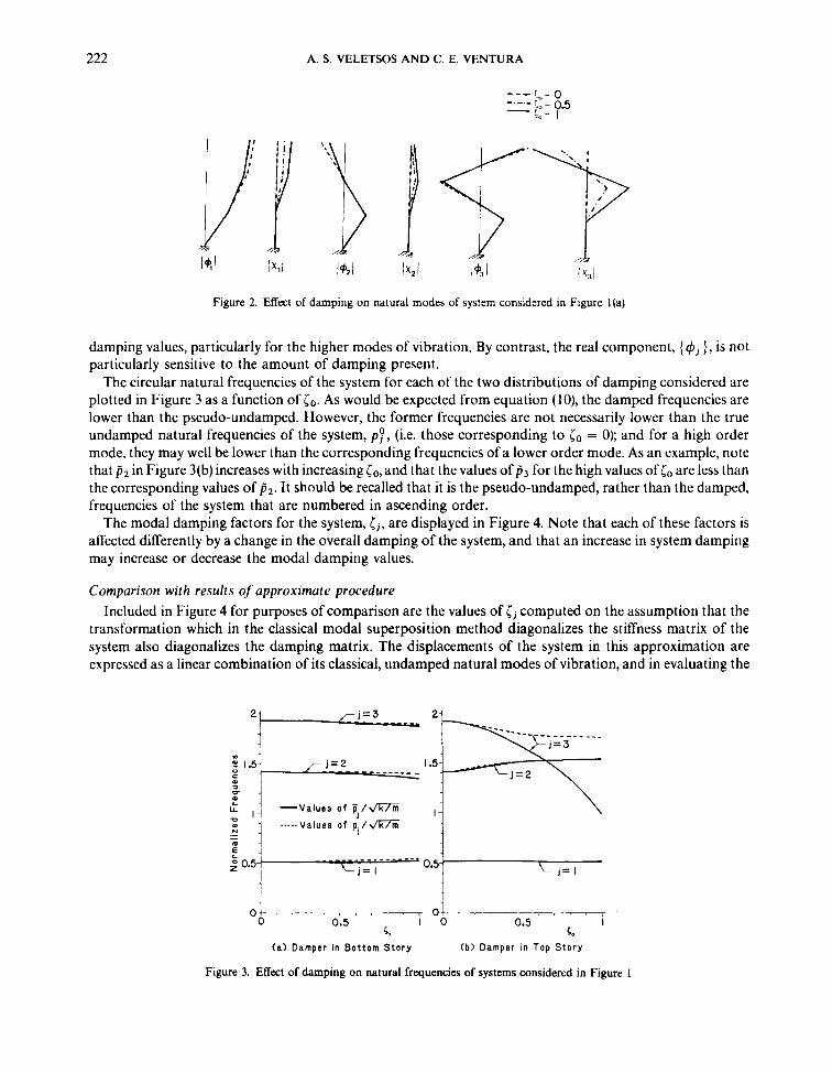
Figure 2. Effect of damping on natural modes of system considered in Figure l(a)

damping values, particularly for the higher modes of vibration. By contrast, the real component, {4 j }, is not particularly sensitive to the amount of damping present.

The circular natural frequencies of the system for each of the two distributions of damping considered are plotted in Figure 3 as a function of lo. As would be expected from equation (lo), the damped frequencies are lower than the pseudo-undamped. However, the former frequencies are not necessarily lower than the true undamped natural frequencies of the system, pj” , (i.e. those corresponding to lo = 0); and for a high order mode, they may well be lower than the corresponding frequencies of a lower order mode. As an example, note that pz in Figure 3(b) increases with increasing lo, and that the values of p3 for the high values of lo are less than the corresponding values of pz . It should be recalled that it is the pseudo-undamped, rather than the damped, frequencies of the system that are numbered in ascending order.

The modal damping factors for the system, l j , are displayed in Figure 4. Note that each of these factors is affected differently by a change in the overall damping of the system, and that an increase in system damping may increase or decrease the modal damping values.

Comparison with results of approximate procedure Included in Figure 4 for purposes of comparison are the values of l j computed on the assumption that the

transformation which in the classical modal superposition method diagonalizes the stiffness matrix of the system also diagonalizes the damping matrix. The displacements of the system in this approximation are expressed as a linear combination of its classical, undamped natural modes of vibration, and in evaluating the

\

O i , _ - - - 0 0.5 I 0 0.5 I

4. c* (a) Damper in Bottom Story (b) Damper in Top Story

Figure 3. Effect of damping on natural frequencies of systems considered in Figure 1


0.5.

E x a c t - ____._ A p p r o x i m a t e

-70.4-

L 0 c

: 0.3 LL

cn c

0 0.5 I 0 0.5 I 5. 5,

(a) D a m p e r in B o t t o m S t o r y (b) D a m p e r i n T o p S t o r y

Figure 4. Effect of damping on modal damping factors for systems considered in Figure I

triple matricial products {&}' [c] { 4 j } , the terms corresponding t o j # k are omitted. The superscript T in the latter expression denotes a transposed vector. This approach, which has been the subject of numerous previous studies,11-14-18 will be referred to herein as the approximate procedure. It may be seen that while the agreement between the two sets of results is generally reasonable, there are significant differences for the system considered in Figure 3(b), particularly for the larger values of lo.

Selected values of the exact and approximate modal damping factors for the system in Figure 1 (a) are listed in Table 11, along with the associated natural frequency values, pi and p j .

MODAL SOLUTION

The term modal solution will be used to identify a solution represented by a linear combination of a complex conjugate pair of characteristic values and their associated vectors. In particular, the j th modal solution for displacements is given by

{x} = C j { $ j ) e r ~ f +Cj{ijj)e5I (1 8) in which C j is a complex-valued constant and Cj is its complex conjugate.

Table 11. Comparison of exact and approximate natural frequencies and damping factors for system considered in Figure l(a)

~~ ~~

Quantity First mode Second mode Third mode Exact Approx. Exact Approx. Exact Approx.

p i / J ( k / r n ) 0.5179 p i / J ( k / m ) 05178

ei 0.0161

p j / J ( k / m ) 05224 p j / J ( k / m ) 05207

e j 00804

05176 05175 00161

05176 0.5 159 00805

05176 05108 01610

(a) eo = 0-1 1.4142 1.4142 1.4138 1.4138 00236 00236

(b) eo = 0.5 1.4127 1.4142 1.4022 1.4044 01221 01179

(c) l o = 1.0 1.3922 1-4142 1.3425 1.3744 02647 02357

1.9312 1.931 I 0.0043

1.9162 1.9159 0.0186

1.8876 1.8870 00241

1.9318 1.9318 00043

1.9318 1.9314 0.02 16

1.9318 1.9300 0.0431


Since the second term on the right-hand member of equation (18) is the complex conjugate of the first, the sum of the imaginary terms in this expression vanishes and equation (18) reduces to

{x} = 2 Re[Cj {t,bj}erj'] (19) in which Re stands for the real part of the quantity that follows.

are considered. If one expresses Cj in terms of its modulus and a phase angle as It is instructive to express equation (19) entirely in real-valued terms, and to this end two alternative forms

c. J = fa.e'O, (20)

and makes use of equations (6) and (9), and of the identity between exponential and trigonometric functions, equation (19) may be written as

{x} = aje-Opif [ { q j j } cos ( p j t + Bj ) - { x i } sin (p i t + O j ) ] (21)

2Cj{t,bj} = {Bj}+i{yj) (22)

Alternatively, if one first evaluates the product

in which i s j } and {yj} are real-valued vectors, then substitutes equation (22) into equation (19), and makes use of the identity between exponential and trigonometric functions, one obtains

{x} = e-~JpJr[{/3j}cospjt -{yj}sinpjt] (23)

Equations (19), (21) and (23) represent the superposition of two exponentially decaying harmonic motions with a circular frequency, pj2 and a damping factor, r j . The component motions lag one another by 90 degrees or one-quarter the period = 2n/p j , and they are in different configurations. As a result, each point of the system undergoes a simple harmonic motion, but the configuration-of the system does not remain constant but changes continuously, repeating itself at intervals 6. The quantity is known as the j th damped natural period of the system.

It should be clear from equation (21) that the { 4 j } configuration is attained when cos(pjt + B j ) = k 1 or sin(pj t + B j ) = 0, whereas the { x j } configuration is attained when sin(pjc + O j ) = k 1 or cos(pjt + O j ) = 0. It can further be seen from equation (23) that the {Bj } configuration is attained when cos p j t = k 1 or sin pjl = 0, whereas the { y j } configuration is attained when sin pit = k 1 or cospj t = 0.

It is important to realize that equations (2l)and (23)are only two ofan infinite number of forms in which the modal solution may be expressed. Other combinations of the basic modal components {qji} and { x j } can be used as the reference configurations, and this fact is used to advantage in a subsequent development.

Reduction for classically damped systems For undamped systems, for which { t , b j } = Gj} = { 4 j } and pj = pj = pj", equation (21) reduces to

{x} = aj{qjj}COS(p~c+8j) (24)

{x} = a j { q j i } e - ~ J p , 0 ~ c o s ( p ~ t + 8 j ) (25)

Such systems can execute simple harmonic motions in fixed, time-invariant configurations. For damped systems satisfying equation (1 l), equation (21) reduces to

in which j jy is related to pi" by the same expression as that relating pi to pj . Such systems can vibrate in time- invariant configurations, but with exponentially decaying amplitudes.

FREE VIBRATION

The response of the system to an arbitrary initial excitation is given by the superposition of the modal solutions presented in the preceding section. In particular, the displacements {XI may be expressed either in the form of equation (19) as

n

{x} = 2 Re[Cj{Jlj}erj'] j = 1


or in the form of equations (21) and (23) as n

{x} = C a j e-cjpj'[ { b j } cos(pjt + o j ) - { x i } sin(pjt + o j ) ] (27) j = 1

or n

{x} = C e-[ipjr [ {~ j}cosp j t -{~ j}s inp j~ ] j = 1

The complex-valued participation factors, C j , may be determined from

in which ( ~ ( 0 ) ) is the prescribed vector of initial displacements and {x(O)} is the corresponding vector of initial velocities. The derivation of this equation is given under the fifth heading in Appendix I. With the values of C j established, the constants a j and 0, in equation (27) are determined from equation (20), and the vectors { B j } and { y j } in equation (28) are determined from equation (22).

For a classically damped system, the following generalized version of equation (14) is valid (see fourth section in Appendix I):

and on making use of this result and of equations (9) and (14), equation (29) reduces to {+jlTE~1 ( ~ ( 0 ) ) = 2t;iPP{4j IT[ml ( ~ ( 0 ) ) (30)

in which

and

Similarly, the vectors { B j } and { y i } in equations (23) and (28) reduce to the well-known expressions:"

in which { 4 j } should be interpreted as the jth real-valued mode of the associated undamped system.

emphasized in the material that follows.

Initial conditions that excite a single mode

Equations (26) and (28) are the more convenient of the three forms used to express the response, and will be

If the initial displacements and velocities of the system are of the form

and

it can be shown (see sixth section in Appendix I) that all values of C j in equation (26), except for the kth, vanish, and that the response of the system is given by

{ X} = 2 Re [ck { $ k } erk']

2 Ck = b,, + id,

(36)

(37)

To clarify the meaning of equations (35), let


in which bk and dk are real-valued constants. On substituting this expression into equations (36)and making use of equation (9), one obtains

{x(o)} = b k { 4 k ) - d k { X k } (384 {x(o)} = b i ( 4 k } - d ; { x k ) (38b)

in which

and

It should now be clear that any initial displacement configuration which is a linear combination of {&.} and { x k ) , along with an initial velocity configuration defined by equations (38b) and (39), will excite only the kth mode of vibration of the system.

In particular, if {x(O)} = b k { & } , the initial velocities needed to excite only the kth mode of vibration are determined from equations (38b) and (39) to be

{%(O)} = - b k ( < k p k { 4 k } + p k { x k ) ) (40) Similarly, if { x(O)} = d { x k } , the corresponding initial displacements are determined from equations (38a) by first computing the values of bk and dk from the system equations (39). The result is

With the proportionality factors bk and dk specified, the values of 2 C k may be determined from equation (37), and the displacements of the system at any time may be determined from equation (36). Alternatively, the displacements may be expressed directly in terms of bk and dk as follows:

1.) = e-ikmf [ (b t { 4 k } - d k { x k } Ices P k t - f d k { + k ) + bk { X k } ) sin p k t ] (42)

Free vibration due to uniform set of initial velocity changes Before proceeding to the analysis of the forced response of the system, it is desirable to re-examine the

response of the system to a uniform set of initial velocity changes with no corresponding displacement changes, i.e. {x(O)} = {0} and {x(O)} = ( l } u o .

Let B j be the value of Cj for a unitary set of initial velocity changes. This value is determined from equation (29) to be

The value of C j for (i(0)) = { l}uo is then C j = Bj uo, and the displacements of the system may be determined from the following expression deduced from equation (26):

n

{x} = 2 C Re[Bj{+j}uoer~r] j = 1

If the product 2Bj{ILj} is now expressed in a form analogous to equation (22) as

in which { f i r ) and { y ) } are real-valued vectors with units of time per radian, equation (44) may also be written in the form


The significance of the superscripts v in the last two expressions is identified later. A simple but crucial final step will now be taken. Let hj ( t ) be the impulse response function for a SDF system,

defined as the response of the system to a unit initial velocity change with no corresponding displacement change. For a viscously damped system with damping factor C j and undamped circular natural frequency p j , this function is given by

and its first derivative is given by

from which, on making use of equation (lo), one obtains

e --W cos pjt = hj( t ) + Cjp jh j ( t ) (49)

The time functions multiplying the vectors { p ; } and { y j } in equation (46) are now replaced by the corresponding expressions defined by equations (47) and (49) to obtain

in which

Arrived at independently in the course of this study, this transformation has also been used recently by Igusa et a].'

Equation (50) is analogous to equation (46) but it differs from the latter in two respects: (a)instead of the sine and cosine functions, it is expressed in terms of the functions h j ( t ) and h j ( t ) which have clear physical meanings; and (b) the reference configurations are the vectors {a;} and {By} instead of the vectors { f i r } and {y;}. In a modal solution, the configuration {a;} is attained at the instant for which hj ( t ) is an extremum, i.e. hj( t ) = 0, whereas the configuration { p;} is attained when h j ( t ) is zero. Equation (50) is fundamental to the analysis of the transient response that follows.

FORCED VIBRATION

The response of the system to an arbitrary excitation of the base may be evaluated from the expressions for free vibration presented in the preceding section as follows. If X,(z) is the acceleration of the base at time t = z, the velocity change of the base in the short time interval between T and 7 +dz is given by Xg(z)d7, and the velocity change of each mass of the structure relative to the moving base is given by u(z) = -X,(t)d~.

The differential displacements ofthe system, {dx},at t > 7 due to these velocitychangesare then given by the following expression, obtained from equation (50) by replacing uo with u(z) and t with t -z:

n

{dx} = - 1 [ { a j } p j h j ( t -z)+ { & } h j ( c -z)]Xg(z)dz j = 1

The displacements of the system due to the prescribed base motion are finally obtained by integration as

in which

and r t


The quantity vj ( t ) in equations ( 5 3 ) and (54) represents the instantaneous pseudovelocity of a SDF system with circular frequency pi and damping factor c j subjected to the prescribed excitation; and Dj( t ) and D j ( t ) represent the corresponding deformation and relative velocity of the system, respectively. It follows that the response of a non-classically damped multi-degree-of-freedom system may be expressed as a linear combination of n pairs of terms. The first member of thejth such pair represents a motion in a configuration { a ; } the temporal variation of which is the same as that of D j ( t ) , whereas the second member represents a motion in a configuration {/I;} the temporal variation of which is the same as that of bj(t). The configurations {a ; } and {/31) are naturally functions of the natural modes of vibration of the system and are defined by equations (45) and (51).

In a stepwise numerical evaluation of the response of a SDF system, the relative velocity, D j ( t ) , is normally computed in the process of obtaining D j ( t ) or the associated pseudovelocity value, Vj(t) . Provided the natural frequencies and modes of a nontlassically damped multi-degree-of-freedom system have been evaluated, therefore, the analysis of such a system may be implemented with only minor computational effort beyond that required for a classically damped system of the same size.

Alternative forms of expressions for response

expressed in terms of D j ( t ) and Dj( t ) , as follows. Instead of the pseudovelocity and true relative velocity functions, Q(t) and bj(t), equation (53) may also be

Let {a?} and { @’} be dimensionless vectors defined by

{ B P I = pi(BT) (56b)

On making use of the relationship between h(t) and D j ( t ) defined by equation (54), equation (53) may then be rewritten as

Similarly, on introducing the vectors

1 1

P j Pi {a t } = - { a ] } = i{af’>

and

and the pseudo-acceleration function, Aj( t ) , defined by

equation (53) can also be written as n

{ X I = 2 [ { a t ) A j ( t ) + {/Ij”)pjDj(t)I (60) j = 1

Eflect of non-zero initial conditions Implicit in the foregoing development has been the assumption that the system is initially at rest. For a

system with non-zero initial conditions, equation (53), or its equivalent versions defined by equations (57) and (60), should be augmented by the addition of the free vibrational solution defined by equations (26), (27) or (28).

Reduction for classically damped systems

satisfy equations (1 5 ) and (16), equation (43) reduces to Bj = - ib;/[2 J( 1 - (3 )], in which For classically damped systems, for which the p j = p y and the natural modes of vibration are real-valued and


From equations (45) and (51) it then follows that { B ; } = {0} and that {a;} = b; {4 j } . Thus, equation (53) reduces to the well-known expression

The v-superscript on the symbol bj emphasizes the fact that the latter quantity is to be used along with the pseudovelocity function, Vj(t) .

Equation (62) can also be expressed in terms of the deformation function, Dj( t ) , as

or in terms of the pseudo-acceleration function, Aj(t), as

in which by and b; are participation factors defined by

and

Summary of procedure

summarized as follows. The steps involved in the analysis of the transient response of a non-classically damped system may be

1. Evaluate the characteristic values, r j , and the associated characteristic vectors, {I,!Ij }; and from equations (5), (7) and (8), determine the damped and pseudo-undamped natural frequencies of the system, pj and pj, and the modal damping factors, c j .

2. From equation (43), compute the participation factors, B j . 3. Evaluate the complex-valued products 2Bj{I,!Ij} = {BJ} +i{yJ}, and by application of equation (51),

compute the vectors {a ; } . Alternatively, one may compute the vectors { a f l and {j?3 from equations (56) or the vectors {a?} and {B?} from equations (58).

4. From analyses of the response of single-degree-of-freedom systems to the prescribed ground motion, determine the pseudovelocity functions, 4(t), and the true relative velocities, D j ( t ) .

5. Compute the displacements {x} from equation (53), and the corresponding storey deformations from

u. I = x. 1 - x . 1 - 1 (66) in which the subscript i refers to the ith floor level or storey. The displacements may also be computed from equation (57) or from equation (60).

Properties of modal response vectors

relations: The vectors { a j } and { B j } with the various superscripts in equations (53), (57) and (60) satisfy the following

i {BJ) = (0) (674 j = 1


and

"

in which {xst} represents the static displacements of the structure due to the inertia forces associated with a uniform structural acceleration of magnitude Zg. These expressions are of great value in checking the accuracy of the solution.

Equation (67a) is deduced from equations (44) and (45) on noting that, for the conditions considered, {x(O)} = (0). Similarly, equation (67b) is obtained from the first derivative of equation (44) by making use of the fact that {x(O)} = { l } . Finally, equation (67c) is obtained by examining the high-frequency limiting behaviour of equation (60). For very stiff systems, the maximum values of {x} tend to {X,~} ; the corresponding values of A j ( t ) and bj(t) tend to -x, and zero, respectively; and equation (60) leads to equation (67c).

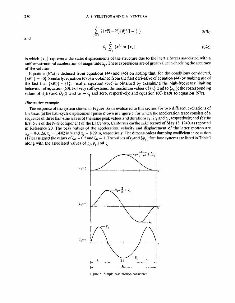
Illustrative example The response of the system shown in Figure l(a) is evaluated in this section for two different excitations of

the base: (a) the half-cycle displacement pulse shown in Figure 5, for which the acceleration trace consists of a sequence of three half-sine waves of the same peak values and durations t l , 2t1 and t,, respectively; and (b) the first 6.3 s of the N-S component of the El Centro, California earthquake record of May 18,1940, as reported in Reference 20. The peak values of the acceleration, velocity and displacement of the latter motion are x, = 0.3 129, xg = 14.02 in/s and x, = 8.29 in, respectively. The dimensionless damping coefficient in equation ( 1 7) is assigned the values of lo = 0.5 and lo = 1. The values of r j and { l(lj } for these systems are listed in Table I along with the associated values of p i , pj and cj .

I- t Figure 5. Simple base motion considered


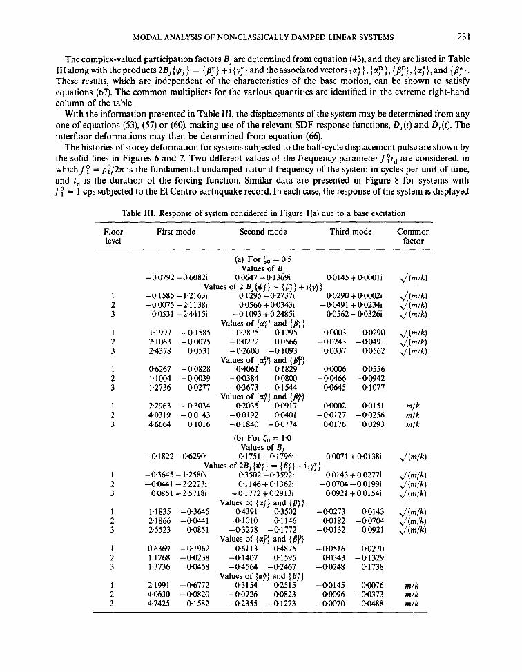
The complex-valued participation factors B j are determined from equation (43), and they are listed in Table I11 along with the products 2 8 , { $ j f = {&> +i{yj') and the associated vectors {a]), {a?}, {By}, {.?),and {B j " } . These results, which are independent of the characteristics of the base motion, can be shown to satisfy equations (67). The common multipliers for the various quantities are identified in the extreme right-hand column of the table.

With the information presented in Table 111, the displacements of the system may be determined from any one of equations (53), (57) or (60), making use of the relevant SDF response functions, D j ( t ) and bj(t). The interfloor deformations may then be determined from equation (66).

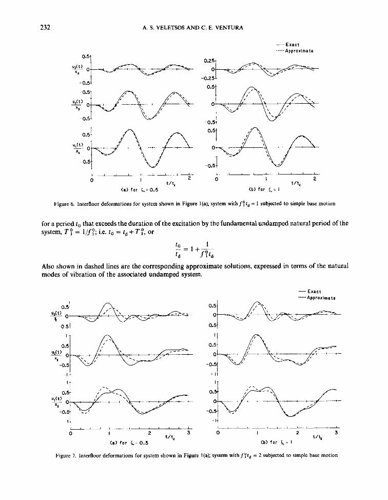
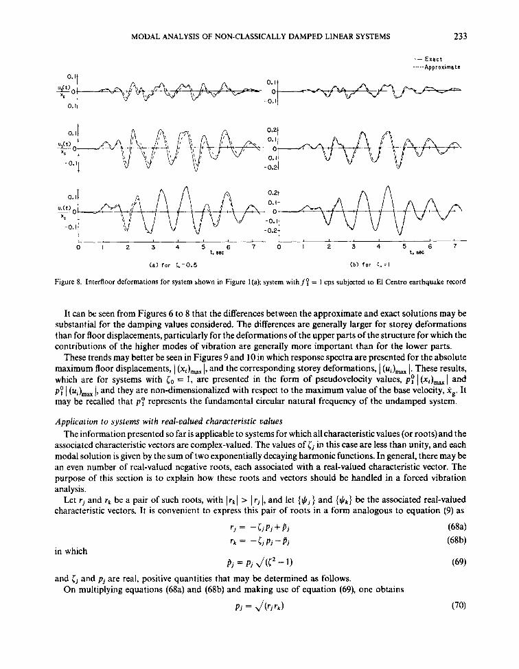
The histories of storey deformation for systems subjected to the half-cycle displacement pulse are shown by the solid lines in Figures 6 and 7. Two different values of the frequency parameter f y t d are considered, in whichf: = py/2n is the fundamental undamped natural frequency of the system in cycles per unit of time, and t d is the duration of the forcing function. Similar data are presented in Figure 8 for systems with f y = 1 cps subjected to the El Centro earthquake record. In each case, the response of the system is displayed

Table 111. Response of system considered in Figure 1 (a) due to a base excitation

Floor First mode Second mode Third mode Common level factor

1 2 3

1 2 3

1 2 3

1 2 3

1 2 3

1 2 3

1 2 3

1 2 3

(a) For c0 = 0 5 Values of Bj

- 0.0792 - 0.60821 0.0647 - 0.1 3691 0.0145 + 0-0001i Values of 2 B j { $ ; ) = (6) +i{yJ}

-0.1585 - 1.2163; 0.1295 -0.27371 0.0290 + 04002i -09075 - 2.1 138i 00566 + 0.0343i -0-0491 +00234i

00531 -2.44151 -01093 +02485i 00562 - 0.03261 Values of {a;' and (61

1.1997 -01585 0.2875 01295 0.0003 00290

2.4378 0.0531 -0.2600 -01093 0.0337 00562

06267 - 0.0828 0.4061 01829 O.oo06 00556

1.2736 00277 -03673 -01544 00645 01077

22963 -03034 0.2035 00917 00002 00151 4.0319 -00143 -00192 00401 -00127 -00256 4.6664 01016 -01840 -00774 00176 00293

2'1063 -0.0075 -0.0272 0.0566 -00243 -00491

Values of {a?} and {By}

1.1004 -00039 -00384 00800 -00466 -00942

Values of {a:) and {#}

(b) For lo = 1.0 Values of B j

- 0 1822 - 0629Oi 0.1751 -0.17961 0.0071 +00138i Values of 2Bj ($1) = {By} + i{yJ}

-0.3645 - 1'258Oi 03502 -0.3592i 00143 + 0.0277i -00441 -2.2223i 0.1 146 + 0 1 3621 -00704 -00199i

00851 -2.5718i -01 772 + 0291 3i 00921 +00154i Values of {a;} and { B; }

1.1835 -0.3645 04391 03502 -00273 00143 2.1866 -00441 -0.1010 0.1146 00182 -00704 25523 00851 -03278 -01772 -0.0132 0.0921

Values of {a?} and { Sf'} 06369 - 0 1962 06113 04875 -00516 00270 1.1768 -00238 -01407 01595 0.0343 - 0 1329 1.3736 00458 -04564 -02467 -00248 01738

Values of {a?} and { Sf} 2.1991 -06772 03154 02515 -00145 00076 4.0630 -00820 -00726 0-0823 0-0096 -00373 4'7425 0-1582 -02355 -01273 -00070 00488

232

-0 5- -0.5~

0.51

A. S. VELETSOS A N D C. E. VENTURA

- E x a c t - - - - - A p p r o x i m a t e

- 0.51

, I I L 1 i I . - 2

t/t, 0 I

<a) for 5.: 0.5

0 I 2

(b) for L o = I t/t,

Figure 6. Interfloor deformations for system shown in Figure I(a); system withfytd = 1 subjected to simple base motion

for a period t o that exceeds the duration of the excitation by the fundamental undamped natural period of the system, T y = l/f y ; i.e. to = t d + T y , or

to 1 - = 1 + 7 'd f l t d

Also shown in dashed lines are the corresponding approximate solutions, expressed in terms of the natural modes of vibration of the associated undamped system.

-I+ I J I J I I I I I I 1 1 ' --.--..--, , I I ' I 1

3 0 I 2 3 t/t, t/t,

0 I

(a) f o r C+,= 0.5 (b) for 6 - I

Figure 7. Interfloor deformations for system shown in Figure I(a); system withfyt, = 2 subjected to simple base motion


F0.. -0. I ,

- E x a c t - - - - -Approximate

0.1.. 0- I -

--0. 1.1

0.1.

~ 0-

-0.1.

U,(t)

XP

i

0.21 0.1

-- 0~

- 0.1.. - 0.21

,,

A 0.24

1 - L 0 I 2 3 4 5 6 7 0 I 2 3 4 5 6 7

t. see rsec (a ) fo r 5.=0.5 (b) t o r 3. = I

Figure 8. Interfloor deformations for system shown in Figure l(a); system withfy = 1 cps subjected to El Centro earthquake record

It can be seen from Figures 6 to 8 that the differences between the approximate and exact solutions may be substantial for the damping values considered. The differences are generally larger for storey deformations than for floor displacements, particularly for the deformations of the upper parts of the structure for which the contributions of the higher modes of vibration are generally more important than for the lower parts.

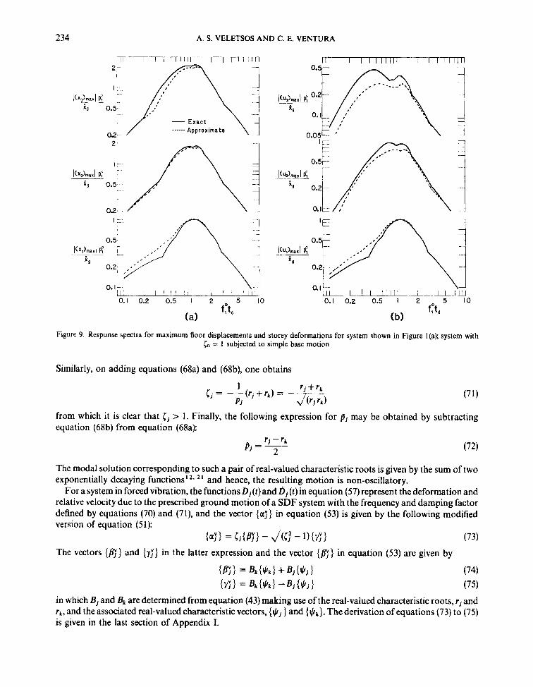
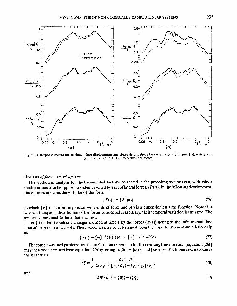
These trends may better be seen in Figures 9 and 10 in which response spectra are presented for the absolute maximum floor displacements, 1 (xi), 1, and the corresponding storey deformations, I 1. These results, which are for systems with co = 1, are presented in the form of pseudovelocity values, p y I (xi)- I and p y 1 ( u ~ ) ~ ~ 1, and they are non-dimensionalized with respect to the maximum value of the base velocity, 1,. It may be recalled that p y represents the fundamental circular natural frequency of the undamped system.

Application to systems with real-valued characteristic values The information presented so far is applicable to systems for which all characteristic values (or roots) and the

associated characteristic vectors are complex-valued. The values of C j in this case are less than unity, and each modal solution is given by the sum of two exponentially decaying harmonic functions. In general, there may be an even number of real-valued negative roots, each associated with a real-valued characteristic vector. The purpose of this section is to explain how these roots and vectors should be handled in a forced vibration analysis.

Let rj and rk be a pair of such roots, with Irk/ > 1 r j 1, and let { $ j 1 and { $ k ] be the associated real-valued characteristic vectors. It is convenient to express this pair of roots in a form analogous to equation (9) as

in which i j j = P j J ( r z - 1)

and Ti and pi are real, positive quantities that may be determined as follows. On multiplying equations (68a) and (68b) and making use of equation (69), one obtains


Figure 9. Response spectra for maximum floor displacements and storey deformations for system shown in Figure 1 (a); system with lo = 1 subjected to simple base motion

Similarly, on adding equations (68a) and (68b), one obtains

r j + rk 1

Pi m C.= J - - ( r j + r k ) = -

from which it is clear that C j > 1. Finally, the following expression for pi may be obtained by subtracting equation (68b) from equation (68a):

r j - rk 2 (72) pj = -

The modal solution corresponding to such a pair of real-valued characteristic roots is given by the sum of two exponentially decaying functions".

For a system in forced vibration, the functions Dj(t)and Dj (t) in equation (57) represent the deformation and relative velocity due to the prescribed ground motion of a SDF system with the frequency and damping factor defined by equations (70) and (71), and the vector {a ; } in equation (53) is given by the following modified version of equation (51):

The vectors { R } and {?I} in the latter expression and the vector {By} in equation (53) are given by

and hence, the resulting motion is non-oscillatory.

= C ~ { B ~ ~ } - J ( C ~ Z - ~ ) { Y ; } (73)

{@} = B k { $ k ) +Bj{$j} (74) {Yr} = B k { $ k / , J - B j { l ( l j } (75)

in which Bi and Bk are determined from equation (43) making use of the real-valued characteristic roots, r j and rk, and the associated real-valued characteristic vectors, {$ j } and { + k ) . The derivation of equations (73) to (75) is given in the last section of Appendix I.


-Exact -----Approximate

i

1

#if 0.05 '

0.2

0. I

1 I 1 1 , 1 I l ! ! I !

5

0. I i/, L U -1

0.05 0.1 0.2 0.5 1 2 f P , C P S (a)

Figure 10. Response spectra for maximum floor displacements and storey deformations for system shown in Figure l(a); system with lo = 1 subjected to El Centro earthquake record

Analysis of force-excited systems The method of analysis for the base-excited systems presented in the preceding sections can, with minor

modifications, also be applied to systems excited by a set of lateral forces, { P ( t ) } . In the following development, these forces are considered to be of the form

{ P ( t ) } = {Plg(t) (76)

in which { P} is an arbitrary vector with units of force and g(t ) is a dimensionless time function. Note that whereas the spatial distribution of the forces considered is arbitrary, their temporal variation is the same. The system is presumed to be initially at rest.

Let ( u ( z ) } be the velocity changes induced at time z by the forces { P ( t ) } acting in the infinitesimal time interval between z and T + dz. These velocities may be determined from the impulse-momentum relationship as

{ u ( z ) } = [m]-'{P(z)}dr = [m]-'{P}g(?)dz (77) The complex-valued participation factor C j in the expression for the resulting free vibration [equation (26)]

may then be determined fromequation (29) by setting {x(O)} = {u (z ) } and {x(O)} = (0). Ifone next introduces the quantities


and follows the steps taken previously in the development of the corresponding solution for base-excited systems, one obtains the following expression for the displacements:

in which

and A j ( t ) is the time derivative of A j ( t ) . The quantity Bj’ in equation (78) and the vectors {aj ’) , I/.?;} and {yj’} in equations (79), (80) and (81) have

units of displacement, whereas the function A j ( t ) is dimensionless. The latter function represents the normalized displacement of a SDF system, the natural frequency and damping factor of which are the same as those of thejth mode of vibration of the prescribed multi-degree-of-freedom system, and is excited by a force of the same temporal variation as g(t). The normalizing factor is the static displacement of the system induced by the peak value of the applied force. Thus

in which X j ( t ) is the displacement of the SDF system and x,, is its maximum static value. The vectors {a?} and { PJ’} in equation (80)are the counterparts of the vectors { a t } and { #’} in equation (60),

and the dimensionless amplification function A j ( t ) is the counterpart of the normalized pseudo-acceleration function, A j (t)/xg.

Application to harmonic response. The steady-state response of non-classically damped systems to a set of harmonic forces may generally be evaluated by direct solution of the governing equations of motion. However, the modal superposition method described in this paper may be preferable for systems having a large number of degrees of freedom, and its application is described briefly in this section.

For exciting forces of the form { P ( t ) } = { P} sin wt (84)

in which w is the circular frequency of excitation, the amplification function Aj ( t ) and its first derivative are given by

A,([) =Ajsin(wt - O j ) and

In the latter expressions, A,([) = ~ A ~ C O S ( C U ~ - O j )

and

0, = tan-’ (3) in which 0 < O j < II.

Let xi([) be the displacement of the ith floor of the system and a$ and B$ be the corresponding values of {aT} and (By) in equation (80). On substituting equations (85a), (85b) and (86b) into equation (go), one obtains

n

xi@) = C Aj[a&sin(ot -f?j)+pjfltcos(wt - O j ) ] (87) j = 1


Further, on expanding the sine and cosine functions and introducing the quantities

tij = ~ j J [ ( a c ) ~ + @jPt)’]

Eij = tan-’ (%) equation (87) may be rewritten as

in which cij is understood to lie in the range 0 to 2n. The maximum value of x i (t) may finally be determined from

Illustrative example. The steady-state response of the system shown in Figure l(a) is evaluated for a harmonic force applied to the first floor level considering T o = 1.

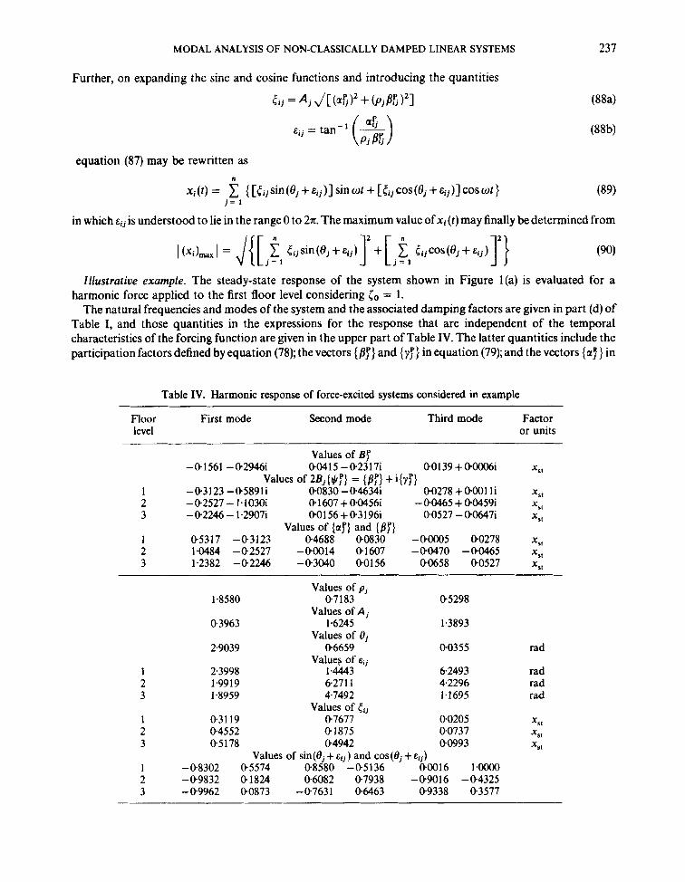
The natural frequencies and modes of the system and the associated damping factors are given in part (d) of Table I, and those quantities in the expressions for the response that are independent of the temporal characteristics of the forcing function are given in the upper part of Table IV. The latter quantities include the participation factors defined by equation (78); the vectors { and {$’) in equation (79); and the vectors {a?) in

Table IV. Harmonic response of force-excited systems considered in example

Floor First mode Second mode Third mode Factor level or units

Values of BIp

Values of 2Bj{$lp} = {BIp} + i{yy} -01561 -02946i 00415 -02317i 001 39 + 0OOO6i XSl

2 -02527 - 1.103Oi 0 1607 + 00456i -00465 + 00459i Xst

3 - 02246 - 1.2907i 0.01 56 + 031961 00527 - 006471 XZ.1

1 05317 -03123 04688 00830 -00005 00278 xst

2 1.0484 -02527 -00014 01607 -00470 -00465 XSt

3 1.2382 -@2246 -03040 00156 00658 00527 XSl

XSl 1 -03123 -05891i 00830 - 04634i 0.0278 + 0001 li

Values of {alp} and {By}

Values of pj 1.8580 07183 05298

Values of A j 0.3963 1.6245 1.3893

Values of 0, 2.9039 06659 00355 rad

Value? of eij 1 2.3998 1 4443 6.2493 rad 2 1.9919 6.27 1 1 4.2296 rad 3 1-8959 4.7492 1.1695 rad

Values of tij 1 03119 07677 00205 X S t

2 04552 0 1875 00737 XSt

3 05178 04942 00993 XSl

Values of sin(Oj+cij) and cos(Bj+cij) 1 -0.8302 05574 08580 -@5136 00016 1~oooO

3 -09962 00873 -07631 06463 09338 03577 2 -09832 01824 06082 07938 -09016 -04325


equation (81). The quantities that do depend on the temporal variation of the exciting force are given in the lower part of Table IV assuming that the value of the exciting frequency w = , /(k/m). The relevant quantities are the frequency ratios, p j ; the amplification factors and phase angles defined by equations (86a) and (86c); the displacement amplitudes and phase angles defined by equations (88); and the values of sin (0, + e i j ) and cos(ej + E i j 1.

The maximum displacements of the system, I (xi)- I, are then determined from equation (90) to be

1 (XI)- 1 = 04471 xSt I ( ~ 2 ) ~ ~ 1 = 04473 xSt 1 ( ~ 3 ) - I = 0*8948~,,

in which x,, = P/k is the static displacement of the first floor due to the peak value of the applied force.

quantities tij by

The results are

The maximum interfloor deformations, 1 (ui)max 1, are determined from equation (90) by replacing the

tij = t i j -ti- I , j (91)

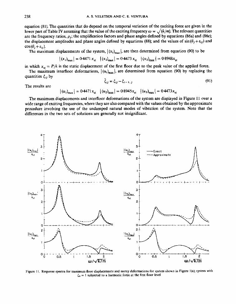
1 (uJ- 1 = 0 4 4 7 1 ~ ~ ~ I ( I ( ~ ) ~ ~ 1 = 0 8 9 4 5 ~ ~ ~ The maximum displacements and interfloor deformations of the system are displayed in Figure 11 over a

wide range of exciting frequencies, where they are also compared with the values obtained by the approximate procedure involving the use of the undamped natural modes of vibration of the system. Note that the differences in the two sets of solutions are generally not insignificant.

I (US)- 1 = 0 . 4 4 7 3 ~ ~ ~

- E x a c t ------ Approxirna t e

3- .. - E x a c t

------ Approxirna t e 2 --

I --

2 t

t

Figure 1 1 . Response spectra for maximum Boor displacements and storey deformations for system shown in Figure 1 (a); system with Co = 1 subjected to a harmonic force at the first floor level


CONCLUSION

With the information arid the physical insight contributed in this paper, the response of a non-classically damped linear system to an arbitrary excitation may be evaluated with only minor computational effort beyond that required for the analysis of a classically damped system of the same size. The response of the system has been expressed in terms of the deformations and true relative velocities of a series of similarly excited single-degree-of-freedom systems.

Comprehensive numerical solutions have been presented for the maximum response of a three-degree-of- freedom system over a range of excitation and system parameters, and the results compared with those obtained by an approximate solution involving the use of classical modes of vibration. It has been shown that, depending on the characteristics of the excitation and of the system itself, the approximate solution may be substantially in error.

ACKNOWLEDGEMENT

This study was supported in part by a research project on the dynamics of offshore structures sponsored at Rice University by Brown and Root, Inc. The project has been under the administrative oversight of Dr. Damodaran Nair, whose cooperation is acknowledged with thanks.

APPENDIX I

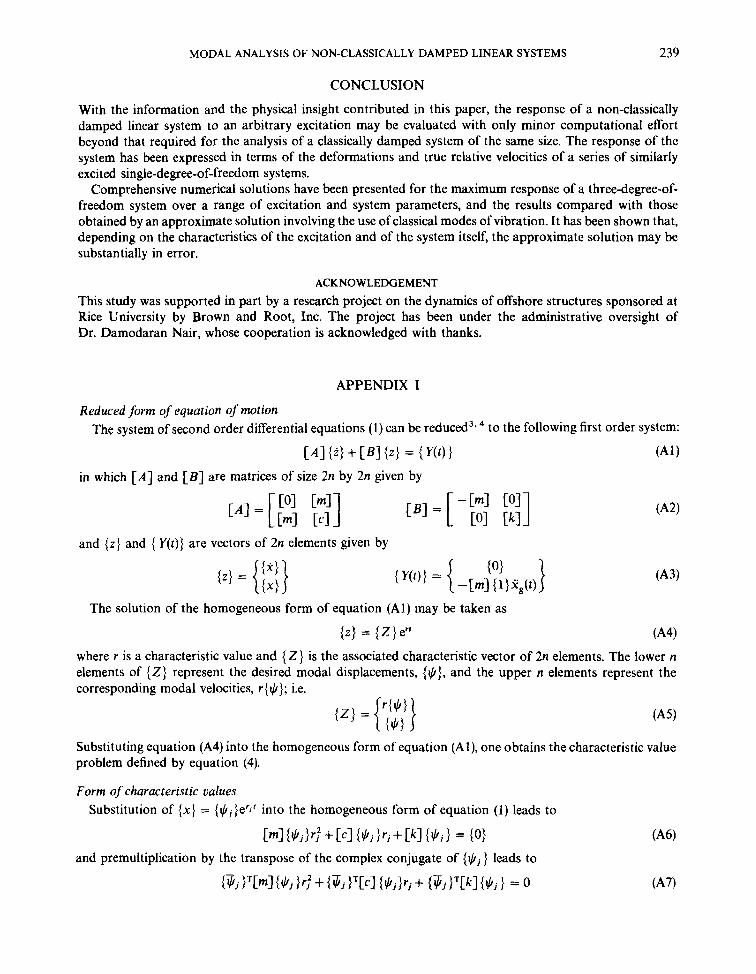
Reduced form of equation of motion The system of second order differential equations (1) can be reduced3. to the following first order system:

[A1 (2) + [BI ( 2 ) = { yo) 1 ('41)

in which [A] and [I?] are matrices of size 2n by 2n given by

and {z) and { Y ( t ) ) are vectors of 2n elements given by

cB1 = [ -Cml [O] [ k ] loll

The solution of the homogeneous form of equation (Al) may be taken as

where r is a characteristic value and { Z} is the associated characteristic vector of 2n elements. The lower n elements of { Z } represent the desired modal displacements, {$}, and the upper n elements represent the corresponding modal velocities, r { $}; i.e.

Substituting equation (A4) into the homogeneous form of equation (Al), one obtains the characteristic value problem defined by equation (4).

Form of characteristic values Substitution of {x} = {$j}erJr into the homogeneous form of equation ( I ) leads to

Cml I$jfri' + C.1 {$j > r j + [kl ($i 1 = { O } and premultiplication by the transpose of the complex conjugate of { $ j f leads to

@ j >"mI {$j >ri' + {7i >'[c] {$j)rj + ( 3 j >'[k] {$j } = 0


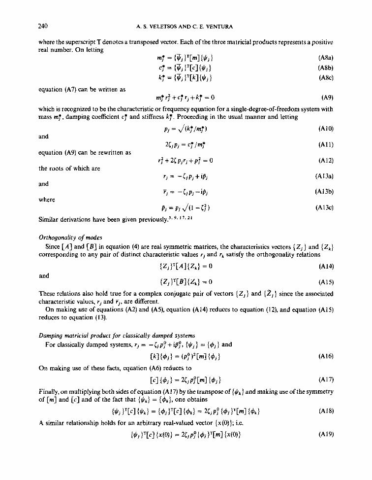
where the superscript T denotes a transposed vector. Each of the three matricial products represents a positive real number. On letting

mf = {7j I'CmI { J l j 1 cf = {7j I'Ccl {$j 1 kf = {7j f'[kl { $ j }

( A W (AW ( A W

equation (A7) can be written as m f r f + c f r j + k f = O

which is recognized to be the characteristic or frequency equation for a single-degree-of-freedom system with mass my, damping coefficient cf and stiffness kf. Proceeding in the usual manner and letting

Pj = J (k f /m~) and

equation (A9) can be rewritten as

the roots of which are

and

where

Similar derivations have been given previou~ly .~~ 9* ''*

2Ljpj = cf /mf

rf+2Lpjrj+pjZ = 0

r j = - l jpj+ipj

Tj = -ijpj-ipj

P j = pj J(1

Orthogonality of modes

corresponding to any pair of distinct characteristic values rj and rk satisfy the orthogonality relations Since [A] and [ B ] in equation (4) are real symmetric matrices, the characteristics vectors { Z j } and {zk}

iZj >'[A] i Z k > = 0 (A 14) and

These relations also hold true for a complex conjugate pair of vectors { Z j } and {z,} since the associated characteristic values, r j and Ti, are different.

On making use of equations (A2) and (A5), equation (A14) reduces to equation (12), and equation (A15) reduces to equation (13).

Damping matricial product for classically damped systems For classically damped systems, rj = - 6 p; + ipy , { I / I j } = { 4j } and

Ckl{4j 1 = (P? )'Em1 {4j 1 On making use of these facts, equation (A6) reduces to

C ~ I { ~ ~ I = ~ C ~ P P C ~ I { ~ ~ } (A17)

Finally, on multiplying both sides of equation (A1 7) by the transpose of {h} and making use of the symmetry of [m] and [c] and of the fact that {$k} = {4k}, one obtains


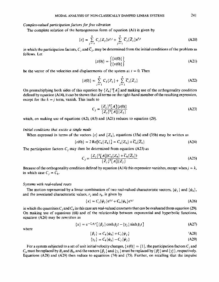
Complex-valued participation factors for free vibration The complete solution of the homogeneous form of equation (Al) is given by

n n

{ z } = C Cj{Zj}erJ'+ C Cj{Zj}eiJ' j = 1 j = 1

in which the participation factors, C j and C j , may be determined from the initial conditions of the problem as follows. Let

be the vector of the velocities and displacements of the system at t = 0. Then

{z(O)} = Cj{Zj}+ C j { Z j } j = 1 j = 1

On premultiplying both sides of this equation by {zk}T[A] and making use of the orthogonality condition defined by equation (A14), it can be shown that all terms on the right-hand member of the resulting expression, except for the k = j term, vanish. This leads to

which, on making use of equations (A2), (A5) and (A21) reduces to equation (29).

initial conditions that excite a single mode When expressed in terms of the vectors {z} and { zk), equations (35a) and (35b) may be written as

{z(o)} = 2Re[Ck{Zk}l = +Ckili(Zk} (A241

The participation factors Cj may then be determined from equation (A23) as

Because of the orthogonality condition defined by equation (A14) this expression vanishes, except when j = k, in which case C j = ck.

Systems with real-valued roots

and the associated characteristic values, rj and rk, is given by The motion represented by a linear combination of two real-valued characteristic vectors, { $ j } and {&},

{x} = cj{+j}erJf +ck{$k}erkr (A261

in which the quantities C j and c k in this case are real-valued constants that can be evaluated from equation (29). On making use of equations (68) and of the relationship between exponential and hyperbolic functions, equation (A26) may be rewritten as

{ x } = e-{jpif [ { Bj } cosh p j t - { y j } sinh p j t ] where

'A28)

(A291

For a system subjected to a set of unit initial velocity changes, (i(0)) = { l}, the participation factors Cj and Ck must be replaced by B j and Bk, and the vectors { B j } and { y j } must be replaced by { E } and {?I}, respectively. Equations (A28) and (A29) then reduce to equations (74) and (75). Further, on recalling that the impulse


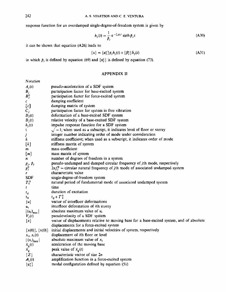
response function for an overdamped single-degree-of-freedom system is given by

1 h j ( t ) = -e-cjPjf sinhpjt

P j

it can be shown that equation (A26) leads to

{x> = { a j ) p j h j ( t ) + {BY)hj(t) in which pi is defined by equation (69) and (a ! } is defined by equation (73).

APPENDIX I1

pseudo-acceleration of a SDF system participation factor for base-excited system participation factor for force-excited system damping coefficient damping matrix of system participation factor for system in free vibration deformation of a base-excited SDF system relative velocity of a base-excited SDF system impulse response function for a SDF system ,,/ - 1; when used as a subscript, it indicates level of floor or storey integer number indicating order of mode under consideration stiffness coefficient; when used as a subscript, it indicates order of mode stiffness matrix of system mass coefficient mass matrix of system number of degrees of freedom in a system pseudo-undamped and damped circular frequency of j th mode, respectively 2nfY = circular natural frequency of j th mode of associated undamped system characteristic value single-degree-of-freedom system natural period of fundamental mode of associated undamped system time duration of excitation

vector of interfloor deformations interfloor deformation of ith storey absolute maximum value of ui pseudovelocity of a SDF system vector of displacements relative to moving base for a base-excited system, and of absolute displacements for a force-excited system initial displacements and initial velocities of system, respectively displacement of ith floor or level absolute maximum value of x i acceleration of the moving base peak value of ig ( t )

characteristic vector of size 2n amplification function in a force-excited system modal configuration defined by equation (51)

t , + T ?


l a 3 {pi}, { y j } {/I;}, {yr} {SF}, {yF} ij modal damping factor i o

{C#J~}, { x i }

modal configuration defined by equation (81) modal configurations defined by equation (22) modal configurations defined by equation (45) modal configurations defined by equation (79)

dimensionless damping coefficient in equation (1 7) real part and imaginary part of j th complex-valued natural mode, {$j}, respectively characteristic vector or natural mode of system

REFERENCES I . T. H. Caughey and M. E. J. OKelly, ‘Classical normal modes in damped linear dynamic systems’, J. appl. mech. A S M E 32,583-588

2. K. A. Foss, ‘Coordinates which uncouple the equations of motion of damped linear dynamic systems’, J. appl. mech. ASME 25,

3 . R. A. Frazer, W. J. Duncan and A. R. Collar, Elementary Matrices, Cambridge University Press, London, 1957. 4. W. C. Hurty and M. F. Rubinstein, Dynamics ofStructures, Prentice-Hall, Clifton, New Jersey, 1964, pp. 313-337. 5. K-Y. Shye and A. R. Robinson, ‘Dynamic soil-structure interaction’, Civil Engineering Studies, SRS No. 484, University of Illinois,

6. M. P. Singh, ‘Seismic response by SRSS for non-proportional damping’, J . eng. mech. dio. ASCE 106, 14051419 (1980). 7. M. P. Singh, ‘Seismic design response by an alternative SRSS rule’, Earthquake eng. struct. dyn. 11, 771-783 (1983). 8. R. W. Traill-Nash, ‘Modal methods in the dynamic analysis of systems with nonclassical damping’, Earthquake eng. struct. dyn. 9,

9. R. Villaverde and N. M. Newmark, ‘Seismic response of light attachments to buildings’, Civil Engineering Studies, SRS No. 469,

(1965).

361-364 (1958).

Urbana, Ill., 1980, pp. 14-33.

153-169 (1981).

University of Illinois, Urbana, Ill., 1980, pp. 108-149. 10. R. W. Clough and J. Penzien, Dynamics OJStructures, McGraw-Hill, New York, 1975, pp. 100-107, 200. 1 1 . W. T. Thomson, T. Calkins and P. Caravani, ‘A numerical study on damping’, Earthquake eng. struct. dyn. 3, 97-103 (1974). 12. J. W. S . Rayleigh, The Theory ofsound, 1st American edn., Dover Publications, New York, 1945. 13. NATS Project, ‘Eigensystem subroutine package (EISPACK)’, A control program for the eigensystem package, Subroutines F269 to

14. Y. D. Beredugo, ‘Modal analysis of coupled motion of horizontally excited embedded footings’, Earthquake eng. struct. dyn. 4,

15. R. W. Clough and S. Mojtahedi, ‘Earthquake analysis considering non-proportional damping’, Earthquake eng. struct. dyn. 4,489496

16. D. L. Cronin, ‘Approximation for determining harmonically excited response of nonclassically damped systems’, J . eng. indust. trans.

17. P. E. Duncan and R. E. Taylor, ‘A note on the dynamic analysis of non-proportionally damped systems’, Earthquake eng. struct. dyn. 7 ,

18. G. B. Warburton and S. R. Soni, ‘Errors in response calculations for non-classically damped structures’, Earthquake eng. struct. dyn. 5,

19. T. Igusa, A. Der Kiureghian and J. L. Sackman, ‘Modal decomposition method for stationary response of nonclassically damped

20. B. Verbic, ‘Analysis of certain structurefoundation interaction systems’, Ph.D. Thesis, Rice University, Houston, Texas, 1972. 21. E. J. Routh, Dynamics o f 0 System ofRigid Bodies, 6th edn., Macmillan, London, 1905 (reprinted by Dover Publications, New York,

F298 and F220 to F247, 1975.

403410 (1976).

(1976).

A S M E 98B, 4 3 4 7 (1976).

99-105 (1979).

365376 (1977).

systems’, Earthquake eng. struct. dyn. 12, 121-136 (1984).

1955).

Modal analysis of non-classically damped linear...

Documents

Transcript of Modal analysis of non-classically damped linear...