7-1996

MOBILE STORMWATER SAMPLING SYSTEM

TO COLLECT STORMWATER SAMPLES AT HIGHWAY SPEEDS DIRECTLY FROM THE

ROAD SURFACE

by

Ernest C. Crosby and

Max Spindler

Technical Report 7-1996-2 Project Number 7-1996

Sponsored by the Texas Department of Transportation

In Cooperation with the U.S. Department of Transportation Federal Highway Administration

February 2003

CIVIL & ENVIRONMENTAL ENGINEERING DEPARTMENT

The University of Texas at Arlington

Arlington, Texas 76019-0308

Technical Report Documentation Page 1. Report No. 7-1996

2. Government Accession No.

3. Recipient's Catalog No.

4. Title and Subtitle Mobile Stormwater Sampling System to Collect Stormwater Samples at

ighway Speeds Directly from the Road Surface H

5. Report Date February 2003

6. Performing Organization Code

7. Author(s) Ernest C. Crosby and Max Spindler

8. Performing Organization Report Technical Report 7-1996-2 10. Work Unit No. (TRAIS)

9. Performing Organization Name and Address Department of Civil and Environmental Engineering The University of Texas at Arlington Arlington, Texas 76019-0308

11. Contract or Grant No. 13. Type of Report and Period Covered Research Report

12. Sponsoring Agency Name and Address Texas Department of Transportation Research and Technology Implementation Office P. O. Box 5080 Austin, Texas 78763-5080

14. Sponsoring Agency Code

15. Supplementary Notes 16. Abstract

A highway stormwater sampling device to facilitate TMDL and NPDES requirements was developed. The

mobile stormwater sampling system collects and samples stormwater from the road surface during storm events. The device can provide a basis for separating direct highway stormwater runoff quality contributions from the total drainage runoff with its highway ancillary drainage contribution. The sampler is unique in that it samples stormwater in real time directly from the roadway surface at traffic speeds during storm events. Stormwater is picked up by a tire, thrown up into the air and collected by a sampler for laboratory analysis.

Additionally, the sampler is coupled with a Global Positioning Satellite (GPS) system, allowing sample

location to be quickly and accurately determined and recorded. The highway stormwater runoff sample analysis can then be transferred to a Geographic Information System (GIS) for spatial reference of data as well as easy data retrieval and useful data recording for study and analyses of highway stormwater quality contributions.

17. Key Words Stormwater, Sampler, Insitu Sampling, Highway Runoff, GIS, GPS, NPDES, TMDL

18. Distribution Statement No restrictions. This document is available to the public through NTIS: National Technical Information Service 5285 Port Royal Road Springfield, Virginia 22161

19. Security Classif. (of this report) Unclassified

20. Security Classif. (of this page) Unclassified

21. No. of Pages

70

22. Price

Form DOT F 1700.7 (8-72) Reproduction of completed page authorized

Mobile Stormwater Sampling System to Collect Stormwater Samples

at Highway Speeds Directly from the Road Surface

by

Ernest C. Crosby Associate Professor

Department of Civil and Environmental Engineering

and

Max Spindler Associate Professor

Department of Civil and Environmental Engineering

Technical Report 7-1996-2 Project Number 7-1996

Research Project Title: Mobile Stormwater Sampling System to Collect Stormwater Samples

at Highway Speeds Directly from the Road Surface

Sponsored by the Texas Department of Transportation

In Cooperation with the U.S. Department of Transportation Federal Highway Administration

February 2003

The University of Texas at Arlington Arlington, Texas 76019-0308

!!!!!!!!!!!!!!!!!!!"#$%!&'()!*)&+',)%!'-!$-.)-.$/-'++0!1+'-2!&'()!$-!.#)!/*$($-'+3!

44!5"6!7$1*'*0!8$($.$9'.$/-!")':!

DISCLAIMER

The contents of this report reflect the views of the authors, who are responsible for the

facts and the accuracy of the data presented herein. The contents do not necessarily reflect the

official view or policies of the Federal Highway Administration (FHWA) or the Texas

Department of Transportation (TxDOT). This report does not constitute a standard,

specification, or regulation. The researcher in charge was Anand J. Puppala, Department of Civil

and Environmental Engineering, The University of Texas at Arlington, Arlington, Texas.

iii

ACKNOWLEDGMENTS

This project is being conducted in cooperation with TxDOT and FHWA. Authors would

like to acknowledge Ms. Dianna Noble, Program Coordinator (PC), Mr. Jay McCurley, Project

Director (PD), and Mr. Tom Remaley, Project Monitor (PM), of the Texas Department of

Transportation, for their interest in and support of this project.

Ernest C. Crosby

Max Spindler

September 2002

iv

TABLE OF CONTENTS

Page

CHAPTER 1 INTRODUCTION................................................................................................ 11.0 Introduction .................................................................................................................... 1

CHAPTER 2 LITERATURE REVIEW.................................................................................... 1

2.0 Sampling Issues .............................................................................................................. 12.0.1 The Clean Water Act .............................................................................................. 12.0.2 Early Studies of Runoff Pollution........................................................................... 22.0.3 Illicit Connection to Storm Sewers ......................................................................... 32.0.4 “First Flush” Runoff .............................................................................................. 32.0.5 Urban Development Effects.................................................................................... 42.0.6 EPA Stormwater Regulations ................................................................................. 52.0.7 Stormwater Samplers .............................................................................................. 5

2.1 Tire Tread........................................................................................................................ 62.3 References....................................................................................................................... 9

CHAPTER 3 TIRE SELECTION and LABORATORY TESTS ........................................... 1

3.0 Laboratory Testing Apparatus........................................................................................ 13.1 Tire Selection for Testing............................................................................................... 23.2 Laboratory Testing ......................................................................................................... 33.3 Sampler Tire Selection ................................................................................................... 6

CHAPTER 4 SAMPLER DESIGN and PLATFORM............................................................ 1

4.0 Trailer and Third Wheel Assembly................................................................................. 14.1 Sampler ........................................................................................................................... 44.2 Intake Collector............................................................................................................... 84.3 Trailer Layout and Decontamination ............................................................................ 104.4 Rain Gauge.................................................................................................................... 10

CHAPTER 5 MOBILE STORMWATER SAMPLER GPS and GIS .................................... 1

5.0 GPS and GIS Components.............................................................................................. 15.1 GPS ................................................................................................................................. 1

5.1.1 Establishing A Data Dictionary ...............................................................................25.1.2 Transferring the Data Dictionary to the Receiver....................................................6 5.1.3 Field Collection with the GPS Receiver. .................................................................7 5.1.4 Downloading the Collected Data To a Computer....................................................8 5.1.5 Differential Correcting the Data ............................................................................10

5.2 GIS ................................................................................................................................ 12 5.3.1 Exporting the Data as an Arcview Shape File .......................................................12

CHAPTER 6 RAINFALL SAMPLING..................................................................................... 1

6.0 Introduction..................................................................................................................... 1 6.1 Sample Locations and Storm Events .............................................................................. 1 6.2 Sample Results................................................................................................................ 3

v

Chapter 7 SUMMARY and RECOMMENDATIONS....................................................... 1 ADDITIONAL REFERENCES................................................................................................... 1

vi

LIST OF FIGURES

Page

Figure 2-1. Tire Tread Design Nomenclature................................................................................ 6 Figure 2-2. Tire Tread Sipes, Blocks, Ribs and Dimples .............................................................. 7 Figure 2-3. Tire Tread Shoulder, Grooving, and Void Ratio......................................................... 7 Figure 2-4. Asymmetrical, Unidirectional, and Symmetrical Tread Patterns................................ 8 Figure 3-1. Tire Spray Simulator Concept .................................................................................. 1 Figure 3-2. Testing Drive Train and Laboratory Simulator ........................................................ 2 Figure 3-3. Tires Tested .............................................................................................................. 3 Figure 3-4. Water Discharge Pattern on Rear Finder.................................................................. 5 Figure 3-5. Tire Speed Versus Motor Setting ............................................................................. 5 Figure 3-6. Tire Testing Results.................................................................................................. 6 Figure 4-1. Third Wheel (Sampling Wheel) in Up Position for Transport ................................. 1 Figure 4-2. Third Wheel in Down Position for Sampling........................................................... 1 Figure 4-3. Third-Wheel-Frame and Rotation ............................................................................ 1 Figure 4-4. Third-Wheel-Frame and Sampling Wheel Axle Attachments ................................. 2 Figure 4-5. Fender and Locking Attachments............................................................................. 3 Figure 4-6. Raising and Lowering Assembly ............................................................................. 3 Figure 4-7. Sample Fender.......................................................................................................... 3 Figure 4-8. Fender Clear Cover Side .......................................................................................... 4 Figure 4-9. ISCO Sampler Mounted on Trailer .......................................................................... 5 Figure 4-10. Top Center Section................................................................................................... 5 Figure 4-11. Peristaltic Pump........................................................................................................ 6 Figure 4-12. Collection Section .................................................................................................... 7 Figure 4-13. ISCO Sampler Collection Hose and Intake Collector .............................................. 7 Figure 4-14. Hose Clamp and Fender Hold Down Close up ........................................................ 8 Figure 4-15. Intake Collector From Rear...................................................................................... 8 Figure 4-16. Intake Collector From Side ...................................................................................... 9 Figure 4-17. Intake Collector from Front...................................................................................... 9 Figure 4-18. Trailer Layout......................................................................................................... 10 Figure 4-19. ISCO 679 Logging Rain Gauge. ..............................................................................11 Figure 5-1. TrimbleGeoExplorer3 .............................................................................................. 1 Figure 5-2. Opening a Data Dictionary....................................................................................... 3 Figure 5-3. Define a New Feature............................................................................................... 3 Figure 5-4. Setting Attribute to Text........................................................................................... 4 Figure 5-5. New Text Attribute................................................................................................... 4 Figure 5-6. New Date Attribute .................................................................................................. 5 Figure 5-7. Summary of Entries.................................................................................................. 5 Figure 5-8. Default Settings Window ......................................................................................... 6 Figure 5-9. Data Transfer ............................................................................................................ 6 Figure 5-10. Geo Explore3 Controls ............................................................................................. 7 Figure 5-11. GeoExplorer3 Window Display .............................................................................. 8

vii

Figure 5-12. Data Files Window................................................................................................... 9 Figure 5-13. Data Transfer Window ............................................................................................. 9 Figure 5-14. Transfer Completed Window ................................................................................... 9 Figure 5-15. Differential Correction Window ............................................................................ 11 Figure 5-16. Confirm Selected Base Files Window.................................................................... 11 Figure 5-17. Export Window ...................................................................................................... 12 Figure 6-1. GIS Regional Map Showing Sampling Locations ................................................... 1 Figure 6-2. Enlarged GIS Map of Sampling Locations .............................................................. 2

viii

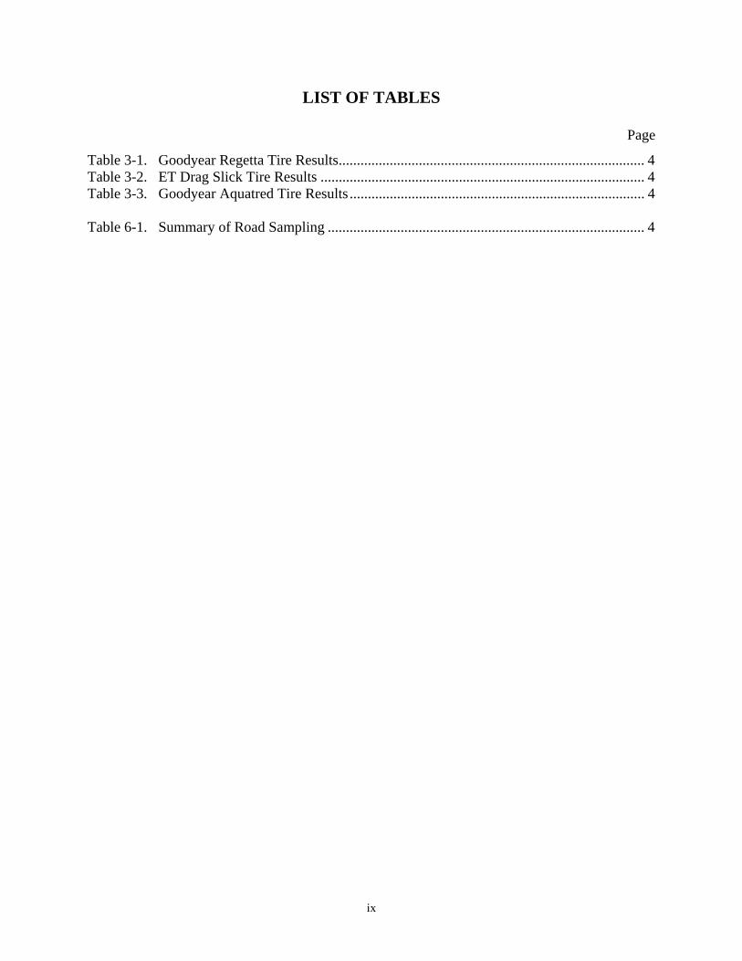
LIST OF TABLES

Page

Table 3-1. Goodyear Regetta Tire Results.................................................................................... 4 Table 3-2. ET Drag Slick Tire Results ......................................................................................... 4 Table 3-3. Goodyear Aquatred Tire Results ................................................................................. 4 Table 6-1. Summary of Road Sampling ....................................................................................... 4

ix

!!!!!!!!!!!!!!!!!!!"#$%!&'()!*)&+',)%!'-!$-.)-.$/-'++0!1+'-2!&'()!$-!.#)!/*$($-'+3!

44!5"6!7$1*'*0!8$($.$9'.$/-!")':!

CHAPTER 1 INTRODUCTION

1.0 Introduction

The objective of this research is to develop a highway stormwater sampling device to

facilitate TMDL and NPDES requirements. Understanding the contribution of stormwater runoff

from highways can be difficult. Normally runoff from stormwater is collected in gutters and

ditches along highways or allowed to commingle with natural drainage leaving the site.

Additionally, it is rare to have highway collection facilities, which collect only roadway drainage

without also receiving runoff from adjoining areas. A tool to collect water samples directly from

the road surface (the source generation point) during storm events would be helpful to establish

actual roadway surface contribution to commingled waters. Structural solutions to this problem

are available. Structural solutions, however, are limited because of their cost and fixed location.

They cannot easily be moved to other locations to investigate or measure the wide varieties of

flow patterns, vehicle mix and highway locations. A mobile system capable of collecting direct

highway runoff and yet be employed on any segment of highway would be useful.

This project investigated, developed and preliminarily evaluated a mobile stormwater

sampling system to collect and sample stormwater from the road surface during storm events.

This device can provide a basis for separating direct highway stormwater runoff quality

contributions from the total drainage runoff with its highway ancillary drainage contribution.

This sampler is unique in that it samples stormwater during real-time events directly from the

roadway surface at traffic speeds. The design is predicated on capturing water picked up by tires

and thrown up into the air. A special device is designed to capture the stormwater while an

automatic sampler collects and stores the samples for later laboratory analysis.

Additionally, the sampler is coupled with a Global Positioning Satellite (GPS) system,

thus allowing sample location to be quickly and accurately determined and recorded. The

highway stormwater runoff sample analysis is then transferred to a Geographic Information

System (GIS) for spatial reference of data as well as easy data retrieval and useful data recording

for study and analyses of highway stormwater quality contributions.

The major project tasks included: 1) literature review; 2) selection of proper vehicle and

tires; 3) design, construction, and testing of collection device; 4) selection of Global Positioning

1 - 1

Satellite receiver and data collection system; and 5) assembling components into a system and

testing the system for functioning and representative sampling.

1 - 2

CHAPTER 2 LITERATURE REVIEW

2.0 Sampling Issues

TxDOT and other DOTs have observed and measured highway runoff for decades to

improve water quality, to research and understand roadway runoff environmental impact, and to

comply with state and federal regulations. Point discharges to water bodies were the original

focus areas of water quality legislation and enforcement. To date, great strides have been made

in point discharge control. Although water quality has improved, continued improvement

necessitates widening the focus to include nonpoint control.

Recent legislation has expanded the NPDES regulations to focus on nonpoint discharges

as well as point discharges. Under this program, increased control of construction sites and

industrial sites during stormwater events is addressed to improve water quality. This has resulted

in increased sampling at catchment outfalls to determine the chemical constituents in nonpoint

runoff. Nonpoint NPDES efforts have led to increased use of structural and non-structural

devices to reduce pollutant loads resulting from roadways and their associated catchments. To

date, the effectiveness of pollutant removal of these devices has been mixed. One of the main

challenges facing DOTs is to clearly distinguish and identify the pollutants of concern that are

generated directly from roadways. Once roadway pollutants contributions are identified and

distinguishable from commingled flow from adjacent roadway areas, appropriate steps can be

investigated to reduce or treat the pollutant loads resulting from roadways at their source.

Section 303 of the Clean Water Act requires that total maximum daily loads (TMDLs) be

determined for all waters in which source effluent limits are not stringent enough to achieve the

water quality standards set for such waters. States and DOTs are attempting to comply with their

TMDL Consent Orders. Both point and nonpoint sources are required to calculate TMDLs.

Clearly identifying the pollutants of concern coming directly from the roadway areas will limit

DOTs’ liability and provide better design insight into pollution prevention and treatment.

2.0.1 The Clean Water Act In 1972 Congress passed the Federal Water Pollution Control Act. This legislation is

often referred to the Clean Water Act (CWA). This law was written to prohibit discharge of

2 - 1

pollutants into waters United States. The legislation's major intent was to prevent a pollutant

discharge from any point source, unless the discharge was authorized by an NPDES (National

Pollutant Discharge Elimination System). The NPDES program is designed to track point

sources and requires the implementation of the controls and monitoring needed to minimize the

discharge of pollutants.

Initially program efforts focused primarily on reducing pollutants in discharges from

easily identifiable sources such as industrial process wastewater and municipal sewage.

Discharges from the sources often lead to serious degradation in water bodies. As pollution

control measures for municipal sewage were implemented and refined, it became evident that

there were many other sources of water quality impairment. Storm water runoff from large

surface areas, such as agricultural and urban land, was identified as a major problem.

2.0.2 Early Studies of Runoff Pollution The National Urban Runoff (NURF) study (1) was the first of its kind to determine the

effective urban runoff on the nation's waters. Conducted from 1978 -1983, it considered 22 urban

and suburban areas nationally. EPA conducted this study to document urban runoff from

residential commercial and industrial areas. It focused mainly on flows from separate storm

sewers. Samples were collected and tested for eight conventional pollutants and the presence of

three heavy metals. Data collected under this study indicated that discharges from separate

storm sewer systems draining runoff from residential, commercial and light industrial areas often

have more than ten times the annual loading of total suspended solids than discharge from

municipal sewer treatment plants. As a result this study indicated that runoff from residential

and commercial areas carried somewhat higher annual loading of chemical oxygen demand and

total copper than effluent from secondary treatment plants. Additionally, the study showed

bacterial and fecal coliform counts in urban areas during the warm weather months, typically

from 10 to 100,000 per milliliter of runoff. The median is around 21,000 per 100 milliliters of

runoff.

The U.S. Geological Survey (USGS) further analyzed this data for 22 Metropolitan areas

(2). USGS summarized the additional monitoring data from the 1980s covering several hundred

storm events at 99 sites and 22 metropolitan areas and documented problems associated with

metals and sediment contamination and urban storm water runoff.

2 - 2

2.0.3 Illicit Connection to Storm Sewers The NURP study found pollutant levels from illicit discharges were high enough to

significantly degrade receiving waters and threaten human, aquatic, and wildlife health. The

study noted that discharges of sanitary waste could be effectively linked to high bacterial counts

in receiving waters.

Illicit discharges to MS4 (Municipal Separate Storm Sewer Systems) sewers can create

severe widespread contamination and water quality problems. Several urban counties have

performed studies to identify and eliminate such discharges.

A Michigan (3) study inspected 660 businesses, homes and other buildings, identifying

approximately 14 percent as having improper storm sewer draining connections. A further

assessment of this program revealed that 60 percent of automobile-related businesses had illicit

connections to storm sewer drains. This assessment also showed that the majority of the illicit

discharges to storm sewer systems resulted from improper plumbing and connections which had

been approved by the local municipality on installation. Inspection of the sewer outfalls revealed

that 32 percent of outfalls had dry weather flows. Of these flows 21 percent were determined to

have pollutant levels higher than was expected in typical urban storm water runoff as

characterized in the NURF study (4).

2.0.4 “First Flush” Runoff Stormwater runoff from lands modified by human activities can harm surface water

resources. Such runoff can cause a water body to fall below state water quality standards. It can

cause a change in the natural hydrologic pattern, accelerating stream flows, destroying aquatic

habitat, and increasing pollutant concentrations and loading. This runoff can contain or carry

high levels of contaminants, such as: sediment, suspended solids, nutrients, heavy metals and

other toxic pollutants, pathogens, toxins, oxygen-demanding substances (organic materials), and

floatable materials (5).

Additionally, runoff carries these pollutants into nearby streams, rivers, lakes, estuaries

wetlands and oceans. The highest concentration of contaminants in runoff is often found in the

first flush discharge. On paved surface pollutants accumulate in dry weather and wash off during

the beginning of the storm. This is why for industrial site concerns, a separate first flush sample

is required along with a flow weighted composite sample. This allows data to be gathered

2 - 3

specifically for the flow periods when pollutants are often at the highest point, while also

showing the total effect the runoff has on receiving waters.

Individually and combined, such pollutants impair water quality, impact pending

designated beneficiary users, and cause habitat alteration or destruction. Uncontrolled storm

water discharges from areas of urban development and construction activities negatively impact

receiving waters by changing the physical, biological and chemical composition of the water.

2.0.5 Urban Development Effects Urban development (7) increases in the amount of impervious surface in a watershed as

farmland, forest, and meadows with natural filtration characteristics, are replaced by buildings

with rooftops, driveways, sidewalks, roads and parking lots. All of these have virtually no

ability to absorb stormwater. Storm water runoff washes over these areas, picking up pollutants,

while gaining speed and volume, because of these areas’ inability to naturally disperse onto or

infiltrate into the ground (8). The resulting flows are higher in volume, pollutant content and

temperature than natural flows, which have more vegetation and soil to slow and absorb runoff.

Studies reveal that the level of impervious cover in an area directly correlates with the quality of

nearby receiving water (9, 10).

In 1996 the EPA 305 (b) Report Inventory (11), a compilation of 60 individual reports,

showed that storm water runoff was a major factor in non-attainment of state water quality

standards; 19 percent of rivers and stream miles; 40 percent of lake, pond, and reservoir acres; 72

percent of estuary square miles; and 6 percent of ocean shoreline waters. This inventory

indicated that approximately 40 percent of the nation's assessed rivers, lakes and estuaries are

impaired, either partially or “not at all” supporting their designated uses.

This 305(b) study also found urban runoff and discharges from storm sewers to be a

major source of water quality impairment nationwide. Nationally these discharges were found to

be a source of pollution in 13 percent of the impaired rivers, 21 percent of the impaired lakes,

ponds, and reservoirs, and 45 percent of impaired estuaries. This ranked second only to

industrial discharges. Obviously, pollutants in stormwater runoff are a prime concern for overall

attainment of state water quality standards.

2 - 4

2.0.6 EPA Stormwater Regulations In 1987, Congress amended the Clean Water Act to require implementation, in a two-

phase comprehensive national program to address storm water discharges. Phase I was

promulgated in November 16, 1990 (55 FR 477990). It requires NPDES permits for storm water

discharges from a large number of priority sources, including Municipal Separate Storm Sewer

Systems (MS4) generally serving populations of 100,000 or more and several categories of

industrial activity including construction sites that disturbed five or more acres (12).

In 1999, Congress implemented the second phase (64 FR 68722) of the program. It

affects principalities of less than 100,000 population. In addition construction sites that impact

less than five acres are now required to institute a set of controls for their storm water runoff.

The initial deadline for the affected groups was extended to March 10, 2003. In addition certain

industries can apply for a no-exposure permit that would eliminate the need for other storm water

related requirements, i.e. best management practices (BMPs) (12).

The Phase II Final Rule ended the temporary exemption from permitting and set deadline

of no later than March 10, 2003, for all ISTA-exempted municipally operated industrial activities

to obtain permit coverage (12).

2.0.7 Stormwater Samplers Extensive literature exists on stormwater pollutant loads and discussions on how to

simulate loads for various conditions. Most city governments such as Los Angeles County,

California (13) and Austin, Texas (14) are addressing NPDES and TMDL requirements by

extensive stormwater monitoring studies. At present, several attempts are being performed to

develop new or adapt old stormwater sampling devices. Hwang (15) is calibrating splitter

flumes as a passive hydraulic device, which divides runoff continuously and delivers it to a

receiving tank where volume flow rate is measured and a composite water sample is collected.

Schaftlein (16) developed a sampling kit to screen and assess potential water pollution problems

from stormwater with global positioning and geographic information system technology. The

sampling kit was found to be ineffective. Dowling (17) developed a low-cost culvert composite

sampler to obtain storm-water sampling. Stein (18) is developing a sheet flow sampler to collect

highway runoff. The above summary shows some of the work that is occurring in this field. No

references were observed indicating work on a mobile roadway surface sampler which collects

the sample at the source.

2 - 5

2.1 Tire Tread

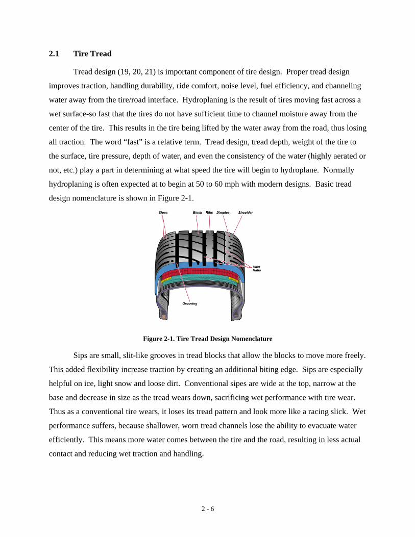
Tread design (19, 20, 21) is important component of tire design. Proper tread design

improves traction, handling durability, ride comfort, noise level, fuel efficiency, and channeling

water away from the tire/road interface. Hydroplaning is the result of tires moving fast across a

wet surface-so fast that the tires do not have sufficient time to channel moisture away from the

center of the tire. This results in the tire being lifted by the water away from the road, thus losing

all traction. The word “fast” is a relative term. Tread design, tread depth, weight of the tire to

the surface, tire pressure, depth of water, and even the consistency of the water (highly aerated or

not, etc.) play a part in determining at what speed the tire will begin to hydroplane. Normally

hydroplaning is often expected at to begin at 50 to 60 mph with modern designs. Basic tread

design nomenclature is shown in Figure 2-1.

Figure 2-1. Tire Tread Design Nomenclature

Sips are small, slit-like grooves in tread blocks that allow the blocks to move more freely.

This added flexibility increase traction by creating an additional biting edge. Sips are especially

helpful on ice, light snow and loose dirt. Conventional sipes are wide at the top, narrow at the

base and decrease in size as the tread wears down, sacrificing wet performance with tire wear.

Thus as a conventional tire wears, it loses its tread pattern and look more like a racing slick. Wet

performance suffers, because shallower, worn tread channels lose the ability to evacuate water

efficiently. This means more water comes between the tire and the road, resulting in less actual

contact and reducing wet traction and handling.

2 - 6

Figure 2-2. Tire Tread Sipes, Blocks, Ribs and Dimples

Blocks are those segments making up a tire’s tread. The primary function of tread blocks

is to provide traction. Ribs are the straight-line row of blocks that create a circumferential

contact “band” with the road surface. Ribs are continuous blocks and have no lateral grooves.

Dimples are the indentations in the tread that improve cooling.

Figure 2-3. Tire Tread Shoulder, Grooving, and Void Ratio

Shoulders provide continuous contact with the road while maneuvering. Shoulders wrap

slightly over the inner and outer sidewall of the tire. Void ratio is the amount of open space in

the tread. A low void ratio means more rubber in contact with the road. A high void ratio

increases the ability to drain water. Whether a tire has a high or low void ratio depends on the

tire’s intended use.

Tire grooving creates voids for better water channeling on wet road surfaces. It is the

most efficient means of channeling water from in front of the tire to behind the tire. By

designing groves circumferentially, water has less distance to be channeled. Circumferential

grooves provide the shortest distance from the front to the rear edges of the contact.

2 - 7

Figure 2-4. Asymmetrical, Unidirectional, and Symmetrical Tread Patterns

Asymmetrical tread pattern changes across the face of the tire. It usually incorporates

larger tread blocks on the outer portion for increased stability during cornering. The smaller

inner tread blocks aid in dissipating water.

Unidirectional tread pattern tires are designed to rotate in only one direction.

Unidirectional tires enhance straight-line acceleration by reducing rolling resistance. They also

provide shorter stopping distance. Unidirectional tires are mounted in the same direction on all

sides of the vehicle, i.e., all tires rotate in the same direction.

Symmetrical tread patterns are deigned to be consistent across the tire’s face. Both

halves of the tread face are the same design.

Both block and rib tread patterns are used in street-tire design. Grooves are used to

create voids within the tread face for better water channeling on wet road surfaces. The most

efficient means of channeling water is between the front and rear edges of the contact patch.

However, lateral grooves help break up the wedge of water that forms at higher speeds. This

reduces the chance of hydroplaning and increases the tire’s contact with the road.

2 - 8

2.3 References

1. U.S. EPA, 1983, Results of the Nationwide Urban Runoff Program, Volume 1 - Final

Report, Office OF Water, Washington, D.C.

2. Driver, N.E., M.H. Mustard, R.B. Rhinesmith, and R.F. Middleburg, Year U.S. Geological

Survey Storm Water Database for 22 Metropolitan Areas Throughout United States, Report

No. 85-337 USGS, Lakewood, CO.

3. Washtenaw County Statutory Board, 1987, Huron River Pollution Abatement Program.

4. U.S. EPA, 1993, Investigation of Inappropriate Pollutant Entries into Storm Drainage

Systems - A User’s Guide, EPA 600/R-92/238, Office of Research and Development,

Washington, D.C.

5. U.S. EPA, 1992, Environmental Impacts of Storm Water Discharges: A National Profile,

EPA 841-R-92-001, Office of Water, Washington, D.C.

6. Schuler, T.R., 1994, “First Flush of Stormwater Pollutants Investigated in Texas”, Note 28,

Watershed Protection Techniques 1 (2).

7. 4 0 CFR Parts 9, 122, 123, and 124, National Pollutant Discharge Elimination System-

Regulations for Revision of the Water Pollution Control Program Addressing Storm Water

Discharges; Final Rule Report to Congress on the Phase II Stormwater Regulations: Notice.

8. U.S. EPA, 1997, Urbanization and Streams: Studies of Hydrologic Impacts, EPA 841-R-97-

009, Office of Water, Washington, D.C.

9. May, C.W., E.B. Welch, R.R. Homer, J.R. Karr, and B.W. May, 1997, Quality Indices for

Urbanization Effects in Puget Sound Lowland Streams, Technical Report No. 154,

University of Washington Water Resources Series.

10. Schueler, T.R., 1994, “The Importance of Imperviousness”, Watershed Protection

Techniques 1(3).

11. U.S. EPA, 1998, The National Water Quality Inventory, 1996 Report to Congress, EPA 841-

R-97-008, Office of Water, Washington, D.C.

12. U.S. EPA, 2000, Storm Water Phase II, Final Rule, An Overview, EPA 833F-00-001, Office

OF Water, Washington, D.C.

13. Depoto, B., M. Ramos, and T. Smith, 1997, “Surface Water Monitoring Under the Country’s

Largest Municipal Stormwater Permit”, Proceedings of the Conference on California and the

2 - 9

World Ocean Proceedings of The 1997 Conference California and The World Ocean, p 24-

27.

14. Brown, T., W. Burd, J. Lewis, and G. Chang, 1994, “Methods and Procedures in Stormwater

Data Collection”, Proceedings Engineer Foundations Conference on Stormwater NPDES

Needs, Aug 7-12.

15. Hwang, R.B., V.M. Pasha, and J. Racin, 1997, “Flume Calibration Process for Continuous

Composite Sampling of Non-Point Runoff”, Proceedings of the Heat Transfer and Fluid

Mechanics Institute, May 29-30.

16. Schaftleing, S., 1996, “Washington State’s Stormwater Management Program”,

Transportation Research Record n 1523 Nov.

17. Doweling, S.J., and D.W. Mar, 1996, “Culvert Composite Sampler: A Cost Effective

Stormwater Monitoring Device”, Journal of Water Resources Planning and Management, V

122, Jul-Aug.

18. Stein, S.M., G.R. Graziano, G.K. Yound, and P. Cazenas, 1998, “Sheetflow Water Quality

Monitoring Device”, Proceedings of the Annual Water Resources Planning and

Management Conference Water Resources and the Urban Environment Proceedings of the

1998 25th Annual Conference on Water Resources Planning and Management, Jun 1-10.

19. Davis, J.R., 2002, “Hydroplanning Issues”, www.msgroup.org/TIP035.html.

20. From Yokohama Rubber Company web site, 2001, www.yokohamatire.com/04a2a.html.

21. From BridgeStone Firestone web site, 2001, www.tirsafety.com/tech.

Note: The Appendix contains additional reference material of interest relating to this

research, which was not directly referenced.

2 - 10

CHAPTER 3 TIRE SELECTION and LABORATORY TESTS

3.0 Laboratory Testing Apparatus

The basic sampler premise originated from observing water thrown up from the roadway

surface by vehicle tires during rainstorms. If this water could be collected in sufficient quantity

and quality, a sampler might be developed to collect runoff directly from the roadway.

A convey belt system was initially investigated to act as a moving roadway to test these

observations in the laboratory and to help study the spray patterns of different tire treads. The

cost of high-speed conveyor belt systems limited it availability for use in this study. The final

test apparatus, created to study water volumes produced from different speeds in the laboratory is

illustrated in Figure 3-1.

TIRE FENDER

RESERVOIR

Figure 3-1. Tire Spray Simulator Concept

The tire is supported by a 6-inch diameter axle, which is slightly submerged in water.

The axle is free wheeling and driven by the tire. Its purpose is to provide tire support and to

provide a base line for water depth. The tire, attached to a truck axle and drive train, is powered

by a variable speed electric motor, as shown in Figure 3-2. A clear plastic fender placed over the

wheel collects water thrown up by the tire and directs it to a collector. The collector located at

the bottom-back of the fender collects the water. The tire and drive train is shown in Figure 3-2.

This arrangement allows tire speeds up to 80 mph.

3 - 1

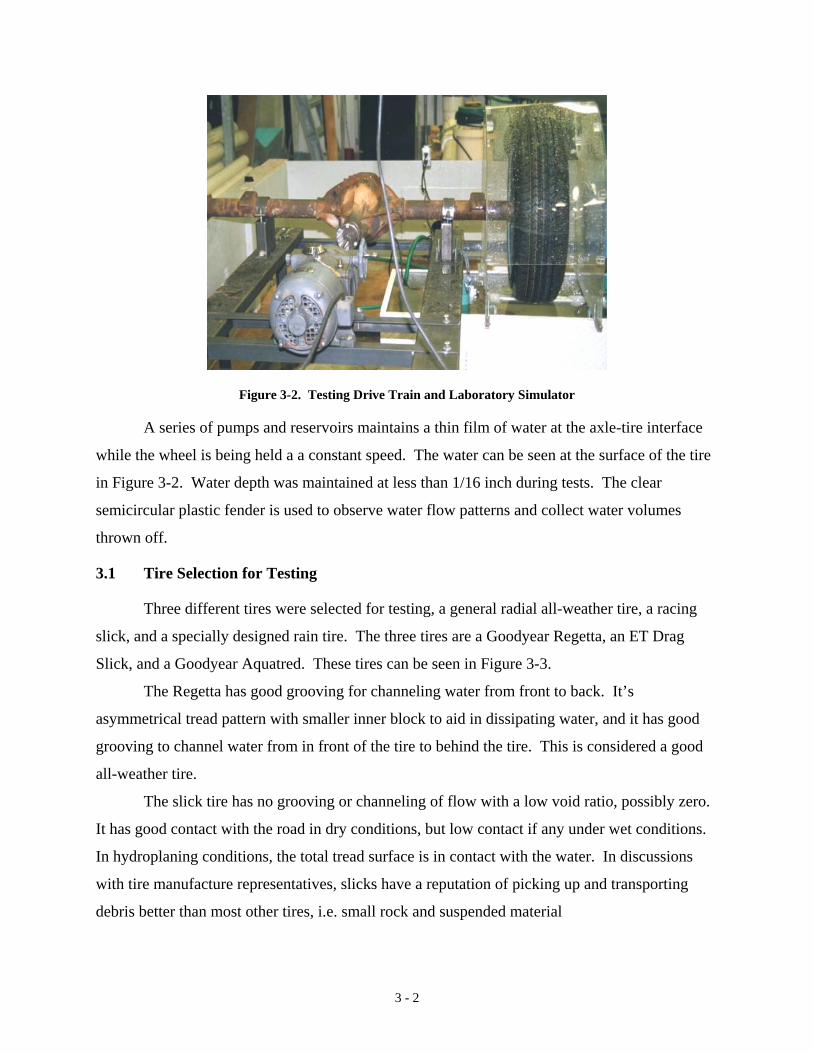
Figure 3-2. Testing Drive Train and Laboratory Simulator

A series of pumps and reservoirs maintains a thin film of water at the axle-tire interface

while the wheel is being held a a constant speed. The water can be seen at the surface of the tire

in Figure 3-2. Water depth was maintained at less than 1/16 inch during tests. The clear

semicircular plastic fender is used to observe water flow patterns and collect water volumes

thrown off.

3.1 Tire Selection for Testing

Three different tires were selected for testing, a general radial all-weather tire, a racing

slick, and a specially designed rain tire. The three tires are a Goodyear Regetta, an ET Drag

Slick, and a Goodyear Aquatred. These tires can be seen in Figure 3-3.

The Regetta has good grooving for channeling water from front to back. It’s

asymmetrical tread pattern with smaller inner block to aid in dissipating water, and it has good

grooving to channel water from in front of the tire to behind the tire. This is considered a good

all-weather tire.

The slick tire has no grooving or channeling of flow with a low void ratio, possibly zero.

It has good contact with the road in dry conditions, but low contact if any under wet conditions.

In hydroplaning conditions, the total tread surface is in contact with the water. In discussions

with tire manufacture representatives, slicks have a reputation of picking up and transporting

debris better than most other tires, i.e. small rock and suspended material

3 - 2

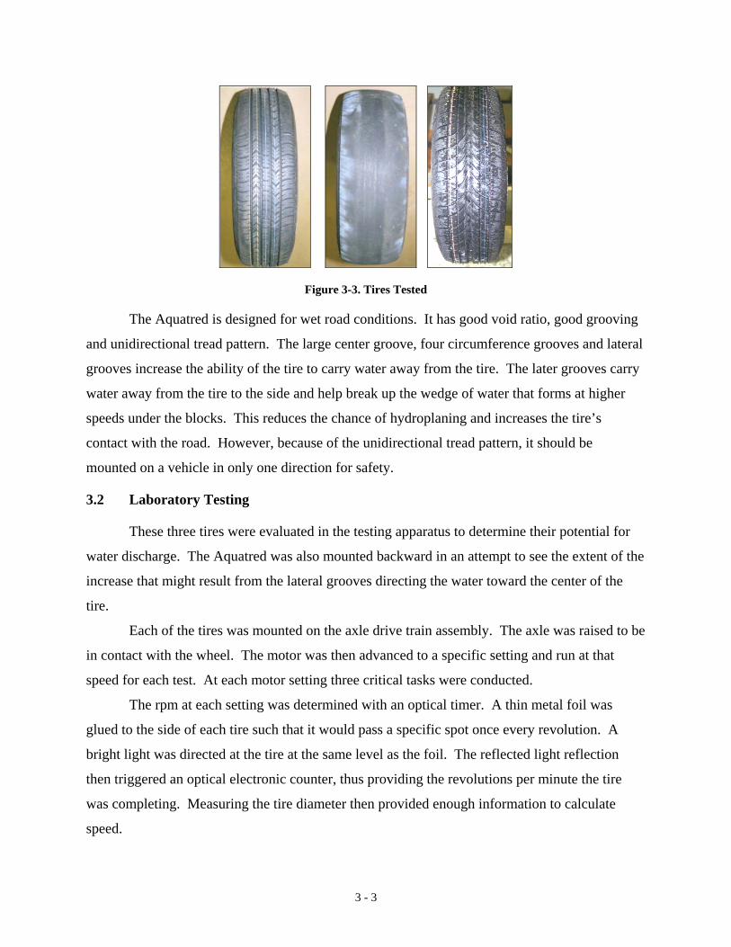
Figure 3-3. Tires Tested

The Aquatred is designed for wet road conditions. It has good void ratio, good grooving

and unidirectional tread pattern. The large center groove, four circumference grooves and lateral

grooves increase the ability of the tire to carry water away from the tire. The later grooves carry

water away from the tire to the side and help break up the wedge of water that forms at higher

speeds under the blocks. This reduces the chance of hydroplaning and increases the tire’s

contact with the road. However, because of the unidirectional tread pattern, it should be

mounted on a vehicle in only one direction for safety.

3.2 Laboratory Testing

These three tires were evaluated in the testing apparatus to determine their potential for

water discharge. The Aquatred was also mounted backward in an attempt to see the extent of the

increase that might result from the lateral grooves directing the water toward the center of the

tire.

Each of the tires was mounted on the axle drive train assembly. The axle was raised to be

in contact with the wheel. The motor was then advanced to a specific setting and run at that

speed for each test. At each motor setting three critical tasks were conducted.

The rpm at each setting was determined with an optical timer. A thin metal foil was

glued to the side of each tire such that it would pass a specific spot once every revolution. A

bright light was directed at the tire at the same level as the foil. The reflected light reflection

then triggered an optical electronic counter, thus providing the revolutions per minute the tire

was completing. Measuring the tire diameter then provided enough information to calculate

speed.

3 - 3

Once the rpm at been established and determined to be constant, the water flow was

adjusted to maintain a constant depth at or above the axle. This was accomplished by adjusting

the pump flow from the reservoirs to balance out the water being lost by tire discharge.

When the system was stable and in equilibrium, a graduated container was placed under

the collector to obtain a volume of discharge equal to 7.4 liters. The time to obtain this volume

was recorded.

Table 3-1. Goodyear Regetta Tire Results

Motor Setting

Observed Revolutions

(rpm)

Tire Speed (mph)

Time (sec)

Discharge (liter/sec)

50 872 72.6 28.19 0.2625 40 698 58.1 35.30 0.2096 30 522 43.5 75.25 0.0983 20 350 29.2 91.31 0.0810 10 173 14.4 179.90 0.0411

Tire Diameter = 14 inches

Table 3-2. ET Drag Slick Tire Results

Motor Setting

Observed Revolutions

(rpm)

Tire Speed(mph)

Time (sec)

Discharge (liter/sec)

50 864 65.5 32.00 0.2313 40 690 52.3 39.50 0.1873 30 518 39.3 77.00 0.0961 20 344 26.1 496.00 0.0149

Tire Diameter = 12.75 inches

Table 3-3. Goodyear Aquatred Tire Results

Motor Setting

Observed Revolutions

(rpm) Tire

SpeedTime (sec)

Discharge (liter/sec)

50 876 70.4 11.00 0.6727 40 702 56.4 12.25 0.6041 30 527 42.3 15.94 0.4642 20 348 28.0 18.30 0.4044 10 178 14.3 24.25 0.3052

Tire Diameter =13.5 inches

3 - 4

Medium and high speed tire water distribution patterns are shown in Figure 3-4.

Figure 3-4. Water Discharge Pattern on Rear Finder

Figure 3-5 shows the variation in motor setting and tire speed. The curves are linear and

show little variation in motor settings and tire speed.

0

10

20

30

40

50

60

70

80

0 10 20 30 40 50Motor Setting

Tire

Spe

ed (m

ph)

GOODYEAR REGETTA ET DRAG 'SLICK' GOODYEAR AQUATRED

Figure 3-5. Tire Speed Versus Motor Setting

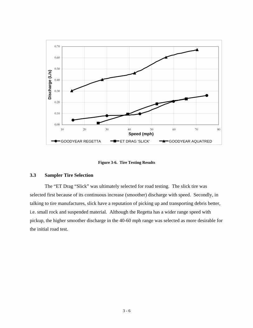
Figure 3-6 shows the variation of tire speed and discharge. The two Goodyear tires both

indicated a tendency at speeds around 40-45 mph to hold discharge constant and then increase.

These two curves appear to be fairly linear otherwise. The Regetta and the Slick have similar

curves with the Slick having a more consistent increase of discharge with velocity. The

Aquatred showed significant increase in discharge potential as compared to the other two tires.

3 - 5

0.00

0.10

0.20

0.30

0.40

0.50

0.60

0.70

10 20 30 40 50 60 70 80Speed (mph)

Dis

char

ge (L

/s)

GOODYEAR REGETTA ET DRAG 'SLICK' GOODYEAR AQUATRED

Figure 3-6. Tire Testing Results

3.3 Sampler Tire Selection

The “ET Drag “Slick” was ultimately selected for road testing. The slick tire was

selected first because of its continuous increase (smoother) discharge with speed. Secondly, in

talking to tire manufactures, slick have a reputation of picking up and transporting debris better,

i.e. small rock and suspended material. Although the Regetta has a wider range speed with

pickup, the higher smoother discharge in the 40-60 mph range was selected as more desirable for

the initial road test.

3 - 6

CHAPTER 4 SAMPLER DESIGN and PLATFORM

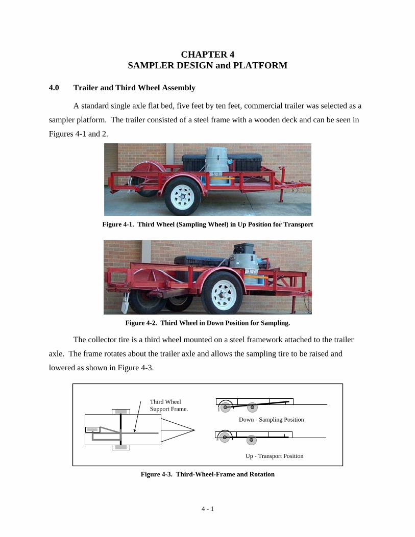
4.0 Trailer and Third Wheel Assembly

A standard single axle flat bed, five feet by ten feet, commercial trailer was selected as a

sampler platform. The trailer consisted of a steel frame with a wooden deck and can be seen in

Figures 4-1 and 2.

Figure 4-1. Third Wheel (Sampling Wheel) in Up Position for Transport

Figure 4-2. Third Wheel in Down Position for Sampling.

The collector tire is a third wheel mounted on a steel framework attached to the trailer

axle. The frame rotates about the trailer axle and allows the sampling tire to be raised and

lowered as shown in Figure 4-3.

Down - Sampling Position

Up - Transport Position

Third Wheel Support Frame.

Figure 4-3. Third-Wheel-Frame and Rotation

4 - 1

The third wheel support frame is made of box steel. It is attached to the axle with u-bolts

and metal races. The races allow rotation about the axle. Stops on the axle keep the third-wheel-

frame from drifting along the axle length. The third-wheel-frame is set to allow the third wheel

to be located in the center of the trailer width, i.e. equidistance from each of the trailer wheels.

The axle for the third wheel is rigidly attached to the last member of the third wheel frame with

u-bolts. The pinning arrangement can be seen in Figure 4-4.

Figure 4-4. Third-Wheel-Frame and Sampling Wheel Axle Attachments

A third tire configuration is used for three basic reasons. First, it allows the sampler

(third wheel) to be transported without contact with the road surface to the place of sampling.

Secondly, it facilitates decontamination of the wheel and fender housing assembly between

sampling events. Finally, this configuration when locked in the down position forms a three-

point contact with the road surface with the sampling wheel being slightly lower than the two

main trailer wheels. This insures that the sampling wheel will be one of the two wheels always

in contact with the roadway surface.

The third-wheel-frame can be locked into a position when the sampling wheel is raised

for transporting. In this position, the frame is locked with a metal safety latch pin in the rear of

the Transporting or Sampling Lock Pin Assembly. See Figure 4-5 for the location of the locking

assembly. When in the sampling position, the frame is locked into the Transporting or Sampling

Lock Pin Assembly at the forward position (see Figure 4-6). This allows continuous pressure on

4 - 2

the tire from the trailer to be in contact with the road. The sampler is raised and lowered into

place manually.

Sampling Fender Attachment Hinges

Transporting or Sampling Lock Pin Assembly.

Figure 4-5. Fender and Locking Attachments

Figure 4-6. Raising and Lowering Assembly

Figure 4-7. Sample Fender

4 - 3

The fender on the sampling wheel is connected to the third-wheel-frame using a set of

hinges that allows it to be raised and lowered to change the wheel, to decontaminate the wheel or

fender between samplings, and to allow the sampling hose to be removed and connected more

easily. Figure 4-5 shows the hinge attachment location on the third-wheel-frame while Figure 4-

7 shows the hinge arrangement.

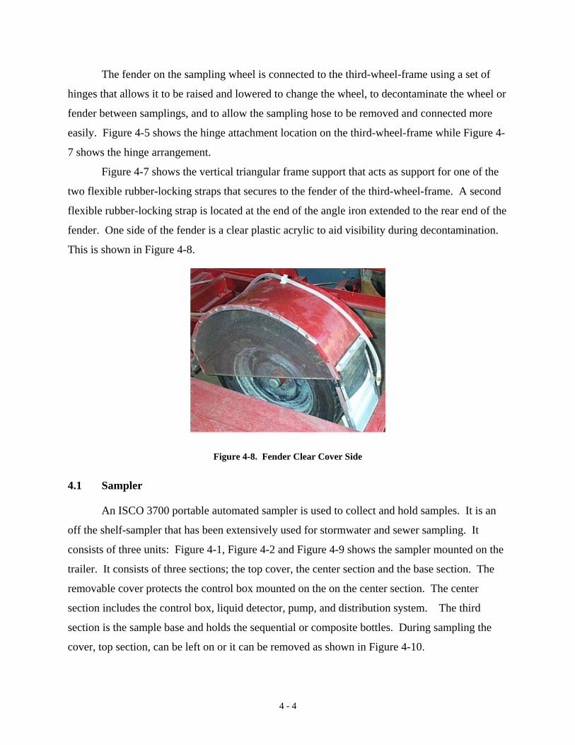
Figure 4-7 shows the vertical triangular frame support that acts as support for one of the

two flexible rubber-locking straps that secures to the fender of the third-wheel-frame. A second

flexible rubber-locking strap is located at the end of the angle iron extended to the rear end of the

fender. One side of the fender is a clear plastic acrylic to aid visibility during decontamination.

This is shown in Figure 4-8.

Figure 4-8. Fender Clear Cover Side

4.1 Sampler

An ISCO 3700 portable automated sampler is used to collect and hold samples. It is an

off the shelf-sampler that has been extensively used for stormwater and sewer sampling. It

consists of three units: Figure 4-1, Figure 4-2 and Figure 4-9 shows the sampler mounted on the

trailer. It consists of three sections; the top cover, the center section and the base section. The

removable cover protects the control box mounted on the on the center section. The center

section includes the control box, liquid detector, pump, and distribution system. The third

section is the sample base and holds the sequential or composite bottles. During sampling the

cover, top section, can be left on or it can be removed as shown in Figure 4-10.

4 - 4

The ISCO 3700 is powered by a12 volt direct current reachable battery, which is attached

to the control box with watertight plug in connections. The watertight connection is the one on

the right in Figure 4-10.

Figure 4-9. ISCO Sampler Mounted on Trailer

A watertight control box mounted on top of this section houses the controller and keypad.

The controller consists of a microprocessor, supporting electronics, and a keypad for input for

automatic or manual control. It displays information, runs the pump, move the distributor,

responds to the keypad and presents information on the display. The controller provides for

manual control of the sampler also. The watertight plug in Figure 4-10 on the right is the remote

control cable. This cable runs to the cab of the towing vehicle and allows the sampler to be

turned off and on from the cab manually.

Figure 4-10. Top Center Section

4 - 5

The sampler is sophisticated in its capability to meet stormwater sampling requirements.

It can program sampling for composite or multiplex sampling, uniform or non-uniform time-

paced sampling, or combinations of these, all automatically and programmed. It can also sample

manually.

This sampler is often used for storm-event sample distribution schemes. The first-flush

sample can be delivered to a single bottle or distributed to several bottles with a multiplexing

scheme. The remaining samples can be distributed to the second bottle group sequentially or

using any of three multiplexing distribution schemes available: bottles-per-sample, samples-per-

bottle or multiple-bottle-composite sample. A sample being the liquid obtained during one

discrete continuous pumping.

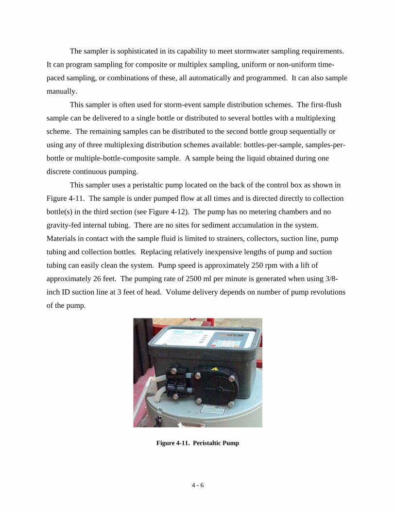
This sampler uses a peristaltic pump located on the back of the control box as shown in

Figure 4-11. The sample is under pumped flow at all times and is directed directly to collection

bottle(s) in the third section (see Figure 4-12). The pump has no metering chambers and no

gravity-fed internal tubing. There are no sites for sediment accumulation in the system.

Materials in contact with the sample fluid is limited to strainers, collectors, suction line, pump

tubing and collection bottles. Replacing relatively inexpensive lengths of pump and suction

tubing can easily clean the system. Pump speed is approximately 250 rpm with a lift of

approximately 26 feet. The pumping rate of 2500 ml per minute is generated when using 3/8-

inch ID suction line at 3 feet of head. Volume delivery depends on number of pump revolutions

of the pump.

Figure 4-11. Peristaltic Pump

4 - 6

The third stage holds the sample bottles. This stage can hold one 2.5-gallon bottle with

insert as shown in Figure 4-12 or one 4-gallon bottle without the insert. Other sample bottle

configurations available are 24 each 1000-ml or 350-ml bottle configuration, 12 each 950-ml

bottle configuration, and 4 each 3800-ml (1-gallon) bottle configuration.

Figure 4-12. Collection Section

When using the different bottle configurations, a device needs to be attached to the pump

outlet on the underside of section 2 to direct the fluid to each bottle. Any use of bottles 1 gallon

or smaller require this Distributor-Arm-Assembly to be used. Preliminary on-road tests with

both the 1 liter and 2.5-gallon bottle configurations reveled (in concurrence with the

manufacture) the smaller opening bottles did not perform well. The sample from the distributor-

arm did not always match well with the mouth of the bottle because of the motion involved. The

larger 2.5 gallon or 4 gallon bottles sit directly under the pump and have close enough proximity

Figure 4-13. ISCO Sampler Collection Hose and Intake Collector

4 - 7

to the discharge that little or no sample is lost while the vehicle is in motion. Accordingly, in the

final road testing, only the 2.5-gallon configuration shown in Figure 4-12 was used.

Flexible 3/8-inch ID tubing (shown in Figure 4-13) is used to connect the ISCO pump to

the collection intake on the third wheel fender housing. This tubing is attached to the third wheel

steel frame and fender with quick release clamps (shown in Figure 4-14) to allow quick change

out of hoses between sampling and assists decontamination. Both the hose and the collection

intake can be seen in Figure 4-13. Attachment of the hose to the sample collector and the pump

are through quick release friction couplers. Figure 4-11 shows the hose connection to the pump.

Figure 4-14. Hose Clamp and Fender

Hold Down Close up

4.2 Intake Collector

The sample intake collector can be seen attached to the sampling hose on the third wheel

in Figure 4-13. The collection intake is fixed to the third wheel fender with a stiff rubber

material to allow some flexibility for impact but resist air drag and potential for planing.

Additionally, a light aluminum frame on the backside provides limited rigidity. This

arrangement can be seen in Figure 4-8 and Figure 4-15.

Figure 4-15. Intake Collector From Rear

4 - 8

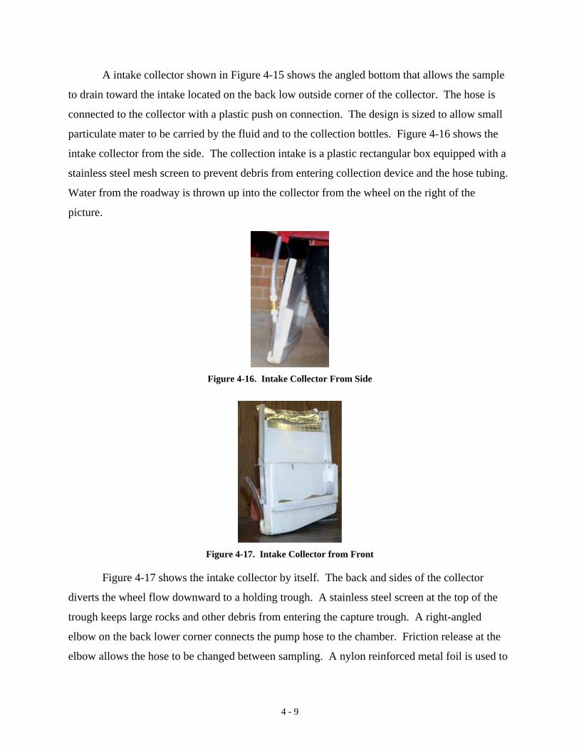
A intake collector shown in Figure 4-15 shows the angled bottom that allows the sample

to drain toward the intake located on the back low outside corner of the collector. The hose is

connected to the collector with a plastic push on connection. The design is sized to allow small

particulate mater to be carried by the fluid and to the collection bottles. Figure 4-16 shows the

intake collector from the side. The collection intake is a plastic rectangular box equipped with a

stainless steel mesh screen to prevent debris from entering collection device and the hose tubing.

Water from the roadway is thrown up into the collector from the wheel on the right of the

picture.

Figure 4-16. Intake Collector From Side

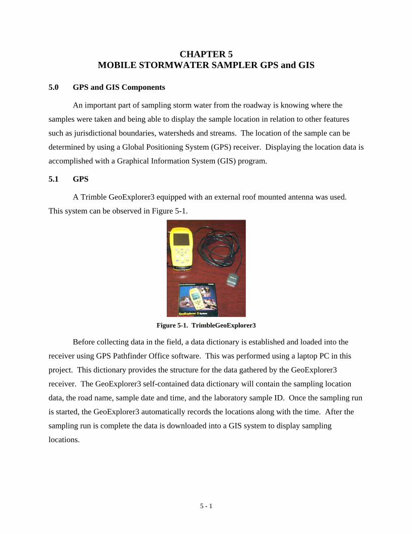
Figure 4-17. Intake Collector from Front

Figure 4-17 shows the intake collector by itself. The back and sides of the collector

diverts the wheel flow downward to a holding trough. A stainless steel screen at the top of the

trough keeps large rocks and other debris from entering the capture trough. A right-angled

elbow on the back lower corner connects the pump hose to the chamber. Friction release at the

elbow allows the hose to be changed between sampling. A nylon reinforced metal foil is used to

4 - 9

cover the hard rubber support on the inside between the fender and the intake collector. This

minimizes the rubber contact with the sample.

4.3 Trailer Layout and Decontamination

Figure 4-10 shows the trailer layout. It includes two storage bins for decontamination

equipment and water, additional sampling bottles and other equipment. A hinged floor access

panel can also be observed adjacent to the third wheel. This allows access to the wheel and

fender for cleaning and decontamination as well as changing and servicing the third wheel.

STORAGE STORAGEACCESS PANEL

ISCO SAMPLER

Figure 4-18. Trailer Layout

Decontamination is an integral part of all sampling. Decontamination between sampling

of road sections is a must to limit cross contamination of samples. The storage boxes on the

trailer store two water sprayers, one with clean water and one with surfactants to clean the tire,

fender, and intake collector. Additionally, clean hose tubes are stored in these boxes for quick

change at different sample.

4.4 Rain Gauge

An ISCO Logging Rain Gauge, model 675 is used to record rainfall at time of sampling.

This is a precision instrument for measuring rainfall that provides accurate measurements from

0.01 - 22 inches per hour. The gauge is mounted inside a cylinder and has an eight inch opening

at the top to collect rain. Rain falls through a screen into a funnel. From the funnel, rain collects

in one side of a two-chambered plastic bucket mounted on jeweled pivots. Rain fills the

chamber, the bucket tips, draining the water and filling the other chamber. When the chamber

fills, the bucket tips back beginning the process begins anew. Each time the bucket tips from on

side to the other, a magnet passes over a reed switch, momentarily closing the contacts. This

contact closure provides a short-duration output pulse from the gauge for each 0.01-inch of rain.

4 - 10

The ISCO 675 Logging Rain Gauge contains a logging device inside the rain gauge that

electronically records and exports the data, via FlowlinkTM software. The logging device has 80

Kb memory, which will provide 900 days of storage at 15-minute intervals or approximately 53

days of storage at 1-minute intervals.

Figure 4-19. ISCO 679 Logging Rain Gauge

The rainfall gauge is battery powered. Its dimensions are 13 inches high and 9.5 inches

in diameter. This gauge needs to be operated in a clear area with no overhang, nor splash up by

other vehicles and be stationary. The gauge is easily transported, small and easily installed in a

minute or two minute. The rain gauge and software package is shown in Figure 19. A laptop PC

or any computer can down load the rainfall data quickly.

4 - 11

!!!!!!!!!!!!!!!!!!!"#$%!&'()!*)&+',)%!'-!$-.)-.$/-'++0!1+'-2!&'()!$-!.#)!/*$($-'+3!

44!5"6!7$1*'*0!8$($.$9'.$/-!")':!

CHAPTER 5 MOBILE STORMWATER SAMPLER GPS and GIS

5.0 GPS and GIS Components

An important part of sampling storm water from the roadway is knowing where the

samples were taken and being able to display the sample location in relation to other features

such as jurisdictional boundaries, watersheds and streams. The location of the sample can be

determined by using a Global Positioning System (GPS) receiver. Displaying the location data is

accomplished with a Graphical Information System (GIS) program.

5.1 GPS

A Trimble GeoExplorer3 equipped with an external roof mounted antenna was used.

This system can be observed in Figure 5-1.

Figure 5-1. TrimbleGeoExplorer3

Before collecting data in the field, a data dictionary is established and loaded into the

receiver using GPS Pathfinder Office software. This was performed using a laptop PC in this

project. This dictionary provides the structure for the data gathered by the GeoExplorer3

receiver. The GeoExplorer3 self-contained data dictionary will contain the sampling location

data, the road name, sample date and time, and the laboratory sample ID. Once the sampling run

is started, the GeoExplorer3 automatically records the locations along with the time. After the

sampling run is complete the data is downloaded into a GIS system to display sampling

locations.

5 - 1

5.1.1 Establishing A Data Dictionary A Data Dictionary provides the basic structure for data gathered by the receiver. In this

type of sampling, the feature is a road represented as a line. Along with the location data, the

road name, sample date and time, and a laboratory sample ID are recorded.

A data dictionary is a description of the features and attributes relevant to a particular

project or job. A data dictionary structures data collection; it does not contain the actual

information collected in the field (positions and actual attribute values for each occurrence of a

feature).

A data dictionary is used in the field to control the collection of features and attributes.

For example, you may want to collect information about power poles, lakes, and roads.

Therefore you can create a data dictionary that contains a list of all these features. It is important

to understand data dictionaries and how they are used in the field to control feature and attribute

collection. A data dictionary prompts you to enter information; it can also limit what you enter

to ensure data integrity and compatibility with your GIS or CAD system.

Although data dictionaries are not always required for field work, they do make

collecting, updating, and processing data easier and faster. A data dictionary consists of the

following elements: 1) A list of features to be collected in the field, and 2)A list of attributes (if

any) that describe each feature.

A data dictionary should contain all the features for which you want to collect

information. You can have different data dictionaries for different projects, for example, one for

each road sampling data dictionary. You can only use one data dictionary at a time in the field.

If you want to collect information about several roads at the same time as information about

utilities, it is important to put all the features into one data dictionary.

The following steps establish a Data Dictionary.

1. Open a new project with pathfinder office

2. From the top pull down menu select Utilities then pull down to Data Dictionary Editor

5 - 2

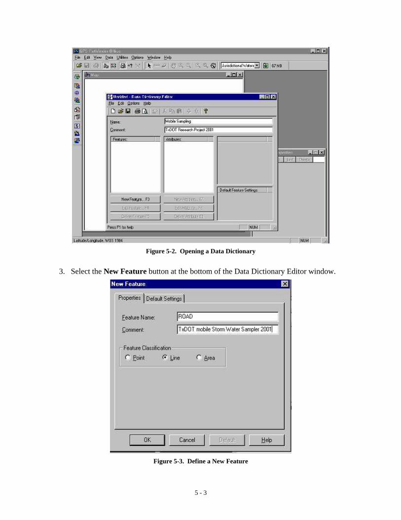
Figure 5-2. Opening a Data Dictionary

3. Select the New Feature button at the bottom of the Data Dictionary Editor window.

Figure 5-3. Define a New Feature

5 - 3

4. In the New Feature window establish the new feature name. For this project we will be collecting a line feature named ROAD.

5. After entering the Feature Name and Feature Classification press OK.

6. Next the Feature Attributes are input. This is accomplished by clicking the New Attribute button on the Data Dictionary Editor window. An attribute must be chosen for each feature. For this project, the feature attributes were the road name, sampling date, sampling time, and lab sample number.

Figure 5-4. Setting Attribute to Text

7. The first attribute is a Text type called Road name. Select Text as the type and click the Add button. Enter “ROAD NAME” as the New Text Attribute.

Figure 5-5. New Text Attribute

8. Repeat steps 6 of the process adding “SAMPLE DATE” as a New Attribute Date type. Select the proper format (Month-Day-Year) and select Auto Generate on Creation. This will cause the receiver to automatically record the date will you are gathering location data.

5 - 4

Figure 5-6. New Date Attribute

9. Repeat step 6 and select a new attribute type of Time. Next the “SAMPLE TIME” is added as a Time type. Once again the proper format is selected along with the Auto Generate.

10. In order to connect the location data with the Water quality analysis done by the laboratory step 6 is repeated and a new attribute type of Text is selected. “LAB SAMPLE ID” attribute is added as a Text type.

11. With the attributes added the Close button is selected. The Data Dictionary Editor summaries the entries.

Figure 5-7. Summary of Entries

12. The Default Feature Settings are shown in the lower right corner of the Data Dictionary Editor. Because data is gathered while the vehicle is in motion, the Log Interval should be set to 1-second intervals. To do this, select Options from the Data Dictionary Editor and Default Feature Settings from the pull down menu. Select the Line tab and the time

5 - 5

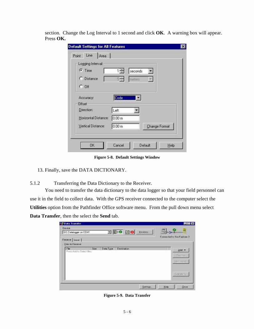
section. Change the Log Interval to 1 second and click OK. A warning box will appear. Press OK.

Figure 5-8. Default Settings Window

13. Finally, save the DATA DICTIONARY.

5.1.2 Transferring the Data Dictionary to the Receiver. You need to transfer the data dictionary to the data logger so that your field personnel can

use it in the field to collect data. With the GPS receiver connected to the computer select the

Utilities option from the Pathfinder Office software menu. From the pull down menu select

Data Transfer, then the select the Send tab.

Figure 5-9. Data Transfer

5 - 6

Select the Add button and Data Dictionary. When prompted select the proper data

dictionary file and Open it. The file will then appear under the Files to send area of the Data

transfer window. Select Transfer All. This will transfer the Data dictionary from the Computer

to the GPS receiver. Close the data transfer window and Exit from Pathfinder Office.

5.1.3 Field Collection with the GPS Receiver. With the Receiver in the vehicle and attached to the external antenna, turn the receiver on

using the button on the lower right side.

Figure 5-10. Geo Explore3 Controls

Listed below are the operational instructions.

1. Press the Data button.

2. Press Down Arrow to highlight file.

3. Press enter.

4. Use the arrow keys and ENTER button to name your file and close.

5. Make sure the proper data dictionary is displayed below the file name.

6. If it is not, use the down arrow to highlight the Data Dictionary and press enter.

7. Highlight the proper Data dictionary and press the enter key.

8. Highlight the Create new file icon and press enter.

9. The receiver will display the file and ask if you want to start logging now or later.

10. Select later.

5 - 7

Figure 5-11. GeoExplorer3 Window Display

11. A new window will appear. Highlight ROAD NAME, press enter, and enter the name of

the road to be sampled using the arrow keys and the enter button, then select close.

12. The date and time can also be changed, but with the Autogenerate function this normally is not required.

13. Use the arrow keys to scroll down to Lab Sample ID and press Enter. Enter a number to connect the lab sample with the location data to be gathered. This number should be used on the laboratory chain of custody, so when the analysis from the lab is complete the location data and sample analysis can be joined.

14. As water sample collection begins, Press the LOG button. The double Bar in the lower right corner of the display should change to a pencil and line indicating that the unit is collecting data. The unit will also beep at the set logging interval. When water sampling is complete, press the LOG button to pause the data collection. Next select, CLOSE. This will store the location data. The receiver will ask for another feature (Road).

15. If multiple samples are to be collected, follow the above procedure to enter ROAD NAME and LAB SAMPLE ID. When data collection is complete, press the CLOSE button and turn the unit off by holding down the POWER on the lower right side of the receiver.

5.1.4 Downloading the Collected Data To a Computer To transfer the data from the GeoExplorer3 to a computer follow the instructions below.

1. Place the Receiver in the cradle and turn it on.

2. Open pathfinder Office.

3. Select the Utilities option from the Pathfinder Office menu. From the pull down menu select Data Transfer, then the Receive tab.

4. Select the Add button and Data Files. When prompted select the proper data file and Open it.

5 - 8

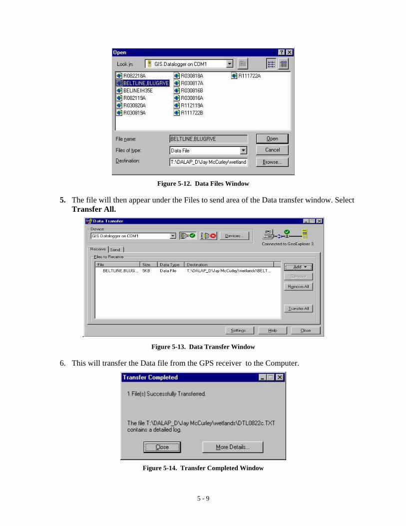
Figure 5-12. Data Files Window

5. The file will then appear under the Files to send area of the Data transfer window. Select Transfer All.

. Figure 5-13. Data Transfer Window

6. This will transfer the Data file from the GPS receiver to the Computer.

Figure 5-14. Transfer Completed Window

5 - 9

5.1.5 Differential Correcting the Data The data has been collected in the field. It has been transferred back to the office

computer and now you need to process it. Unless you collect the field data using a real-time

differential source, the data will only be accurate to about 100 meters due to the effects of

Selective Availability (SA). In some cases this may be adequate, but for most applications a

much better level of accuracy is required.

You can significantly improve the accuracy of field data through a process called

Differential Correction. This requires a set of ‘base’ files that are collected at a known location

at the same time that the field data files are collected. Many regions have Community Base

Stations or Trimble Reference Stations that can supply this base data, or you can use a second

data logger to collect your own base data. This allows the data to be accurate to about 1 m.

To correct the data for TxDOT follow the following steps.

1. From the TxDOT website www.dot.state.tx.us/ select the Customer Services section and click on Global Positioning System Data. Under the Global Positioning System Data section click where it says Click Here. Select the month when you were gathering data.

2. On the next screen select the base station nearest to the location you were gathering the location data.

3. Down load the file(s) corresponding to when the data was collected and save them to your Base folder.

4. Close the browser.

5. These files are compressed and should be extracted. Select the Utilities option from the Pathfinder Office menu. From the pull down menu select Differential Correction.

6. If your location data file does not appear in the Rover file window, use the browse button to select the proper file. The base file can be selected either by the search button or the Browse button.

7. The following box should appear with the rover files and base files. Select the OK button.

5 - 10

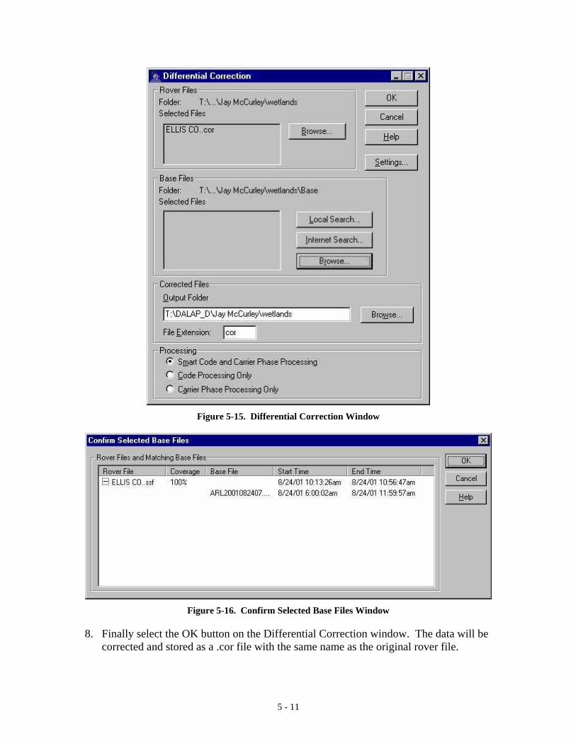
Figure 5-15. Differential Correction Window

Figure 5-16. Confirm Selected Base Files Window

8. Finally select the OK button on the Differential Correction window. The data will be corrected and stored as a .cor file with the same name as the original rover file.

5 - 11

5.2 GIS

The result of many GPS data collections is to incorporate the data into a database, such as

a spreadsheet or a GIS. Depending on the database that you use, you must export your collected

and edited data files in a format that your end-product software can use. The GPS Pathfinder

Office software supports a variety of major GIS, CAD, and spatial database formats. It also lets

you define your own ASCII formats.

Arcview shape files were selected to produce maps showing the location of the data

acquisition.

5.3.1 Exporting the Data as an Arcview Shape File Select the Utilities option from the Pathfinder Office software menu. From the pull down menu select Export.

Figure 5-17. Export Window

5 - 12

CHAPTER 6 RAINFALL SAMPLING

6.0 Introduction

After initial component testing of the sampler, four rain event samplings of roadways

were made during rainstorm events. The roadways sampled consisted of two sections of

Interstate Highway 30 and a local concrete thoroughfare. After collection, the samples were sent

to a commercial testing facility for analysis. Only those constituents presently required by

regulation for the local TxDOT area were investigated. The sampling results were then

compared to runoff observed in local creeks and recorded by local area authorities.

6.1 Sample Locations and Storm Events

Four roadway sections were selected for sampling. Figure 6-1 shows the road site

locations in yellow as recorded by the GPS and displayed on a regional map using GIS.

I.H. 30

Abrams Street

Figure 6-1. GIS Regional Map Showing Sampling Locations

The roadway sampling locations are as follows.

Abrams Street was sampled from Fielder Road west to Bowen Road, a distance of

approximately 1.1 miles. This roadway was just constructed and consisted of a curbed 4-lane

6 - 1

concrete road. The west bound outside lane adjacent to the curb was sampled. It was sampled

on March 8, 2001. This roadway section is identified on Figure 6-2 as site (1). This site was

sampled during the first part of a late morning storm.

Interstate Highway 30 was sampled from Fielder Road exit east bound to Cooper Street, a

distance of approximately 0.8 miles. The pavement was concrete with 3-lanes of traffic east

bound and a paved shoulder. The east bound outside lane adjacent to the shoulder was sampled.

It was sampled on February 15, 2001. Identified as site (2) in Figure 6-2. This storm was

sampled during the first part of an afternoon storm.

Interstate Highway 30 was sampled from Ballpark Way exit west bound to Collins Street,

a distance of approximately 1.3 miles. The pavement was concrete with 3-lanes of traffic west

bound and a paved shoulder. The west bound outside lane adjacent to the shoulder was sampled.

Site is identified as site (3) in Figure 6-2. It was sampled on March 8, 2001. Site (3) and (4)

were sample contiguously, one after the other during an early afternoon storm. They represented

the first part of the storm.

Interstate Highway 30 was sampled from Collins Street exit east bound to Ballpark Way,

a distance of approximately 1.4 miles. The pavement was asphalt surface treatment with 3-lanes

of traffic west bound and a paved shoulder. The east bound outside lane adjacent to the shoulder

was sampled. Site is identified as site (4) in Figure 6-2. It was sampled on March 8, 2001. Site

(3) and (4) were sample contiguously, one after the other. They represented the first part of the

storm.

(3) (2) (4)

I.H. 30

Abrams Street

(1)

Figure 6-2. Enlarged GIS Map of Sampling Locations

Figure 6-2 shows an enlarged GIS display of the sampling locations. The yellow lines

indicate the GPS tracked sampling locations along the roadways. The numbers in parenthesis

references the sampler roadways. Sites (3) and (4) show more roadway than was sampled

6 - 2

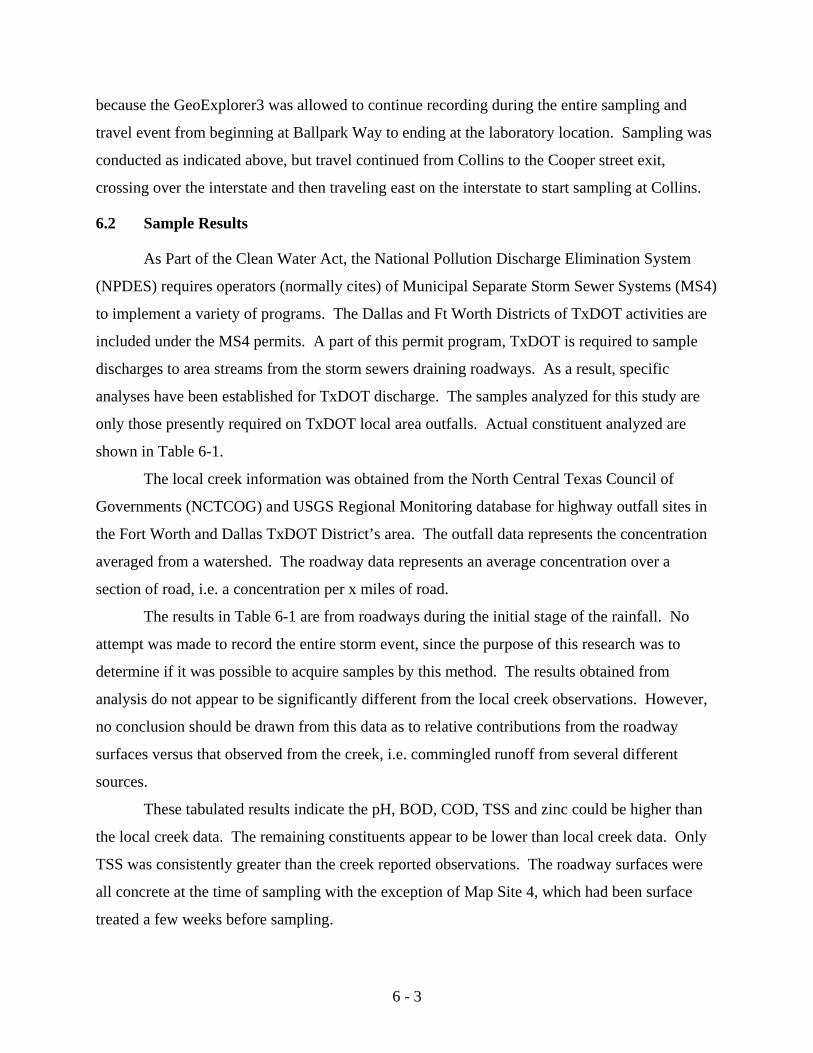
because the GeoExplorer3 was allowed to continue recording during the entire sampling and

travel event from beginning at Ballpark Way to ending at the laboratory location. Sampling was

conducted as indicated above, but travel continued from Collins to the Cooper street exit,

crossing over the interstate and then traveling east on the interstate to start sampling at Collins.

6.2 Sample Results

As Part of the Clean Water Act, the National Pollution Discharge Elimination System

(NPDES) requires operators (normally cites) of Municipal Separate Storm Sewer Systems (MS4)

to implement a variety of programs. The Dallas and Ft Worth Districts of TxDOT activities are

included under the MS4 permits. A part of this permit program, TxDOT is required to sample

discharges to area streams from the storm sewers draining roadways. As a result, specific

analyses have been established for TxDOT discharge. The samples analyzed for this study are

only those presently required on TxDOT local area outfalls. Actual constituent analyzed are

shown in Table 6-1.

The local creek information was obtained from the North Central Texas Council of

Governments (NCTCOG) and USGS Regional Monitoring database for highway outfall sites in

the Fort Worth and Dallas TxDOT District’s area. The outfall data represents the concentration

averaged from a watershed. The roadway data represents an average concentration over a

section of road, i.e. a concentration per x miles of road.

The results in Table 6-1 are from roadways during the initial stage of the rainfall. No

attempt was made to record the entire storm event, since the purpose of this research was to

determine if it was possible to acquire samples by this method. The results obtained from

analysis do not appear to be significantly different from the local creek observations. However,

no conclusion should be drawn from this data as to relative contributions from the roadway

surfaces versus that observed from the creek, i.e. commingled runoff from several different

sources.

These tabulated results indicate the pH, BOD, COD, TSS and zinc could be higher than

the local creek data. The remaining constituents appear to be lower than local creek data. Only

TSS was consistently greater than the creek reported observations. The roadway surfaces were

all concrete at the time of sampling with the exception of Map Site 4, which had been surface

treated a few weeks before sampling.

6 - 3

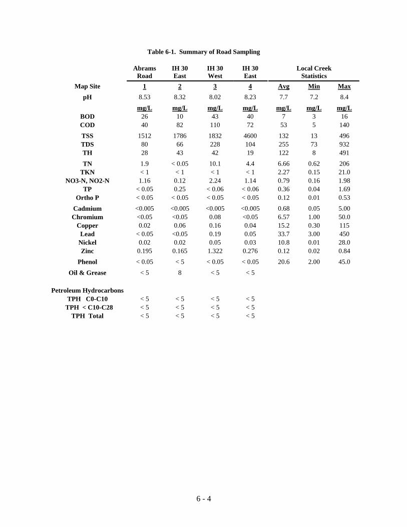
Table 6-1. Summary of Road Sampling

Abrams Road

IH 30 East

IH 30 West

IH 30 East

Local Creek Statistics

Map Site 1 2 3 4 Avg Min MaxpH 8.53 8.32 8.02 8.23 7.7 7.2 8.4

mg/L mg/L mg/L mg/L mg/L mg/L mg/LBOD 26 10 43 40 7 3 16 COD 40 82 110 72 53 5 140

TSS 1512 1786 1832 4600 132 13 496 TDS 80 66 228 104 255 73 932 TH 28 43 42 19 122 8 491

TN 1.9 < 0.05 10.1 4.4 6.66 0.62 206 TKN < 1 < 1 < 1 < 1 2.27 0.15 21.0

NO3-N, NO2-N 1.16 0.12 2.24 1.14 0.79 0.16 1.98 TP < 0.05 0.25 < 0.06 < 0.06 0.36 0.04 1.69

Ortho P < 0.05 < 0.05 < 0.05 < 0.05 0.12 0.01 0.53

Cadmium <0.005 <0.005 <0.005 <0.005 0.68 0.05 5.00 Chromium <0.05 <0.05 0.08 <0.05 6.57 1.00 50.0

Copper 0.02 0.06 0.16 0.04 15.2 0.30 115 Lead < 0.05 <0.05 0.19 0.05 33.7 3.00 450

Nickel 0.02 0.02 0.05 0.03 10.8 0.01 28.0 Zinc 0.195 0.165 1.322 0.276 0.12 0.02 0.84

Phenol < 0.05 < 5 < 0.05 < 0.05 20.6 2.00 45.0

Oil & Grease < 5 8 < 5 < 5

Petroleum Hydrocarbons TPH C0-C10 < 5 < 5 < 5 < 5

TPH < C10-C28 < 5 < 5 < 5 < 5 TPH Total < 5 < 5 < 5 < 5

6 - 4

Chapter 7 SUMMARY and RECOMMENDATIONS

This research developed a first generation sampler, which is capable of sampling directly

from the roadway surface during storm events at typical driving speeds. The staging platform for

this sampler is small commercial flatbed trailers equipped with a third wheel, which channels

water that the tire throws up to an intake collector. The water is then pumped via a peristaltic

pump to a composite collection bottle for transport to a lab and ultimate analysis at a laboratory.

At the same time the sample is being collected a GPS system is recording the location of the

sample, which is input to a GIS system along with the laboratory analysis for management and

record needs.

The result of this research is the verification of the feasibility concept of a sampler,

picking up water from roadway surface while traveling at highway speeds. One working

prototype sampler has been delivered to the TxDOT Dallas District Office.

A likely outcome of this research is the ability to isolate direct contribution of stormwater

runoff from any surface section of highway without extensive investment in structures to capture

the needed samples.

As with all first generation samplers, enhancements and improvements can improve

usability and reliability. Outlined below are several items that could assist implantation of this

sampler.

Stormwater sampling guidelines at present separate MS4 stormwater sampling into two

parts, “First Flush” composite sample and latter storm samples collected in sequential, composite

or multiplexing type samples. This research used “first flush” composite type sampling. To be

compatible with MS4 requirements, a protocol should be established which is compatible to MS4

and NPDES stormwater sampling. This research used a sophisticated off-the self stormwater

sampler that had the capability to perform the above varied types of sampling. However, it was

quickly discovered that this sophisticated programmable sampler capabilities could only be used

for a non moving platform. This is a result of the method used to divert flow from one bottle to

another for other than composite sampling protocols. A potential solution is to replace the costly

sophisticated programmable peristaltic pump with a bank of simple inexpensive peristaltic

pumps. This would allow each pump to collect a separate composite sample, multiple composite

samples, or multiplex the samples as presently done, i.e. instead of directing the flow with a

7- 1

moveable arm, redirect the flow with a bank of pumps. This could be accomplished with one

hose to the intake collector and a gang of valves arranged between the hose and the pumps. This

type of arrangement easily lends itself to a simple electric switch control from remote locations

such as the cab of the truck pulling the sampler. Presently programmable pumps available off

shelf are programmed by timing the pump and not by measuring the flow. As a result, simple

pumps that directly discharge into the sampling containers could provide significant cost

reductions. This cost saving would allow several simple pumps to be mounted as a bank of

pumps each run independently.

In addition, additional sampling under controlled conditions should be performed to

assure that there is no statistically difference between this type of sampling and present sampling

techniques, i.e. such as curb sample collection were no commingling of flows can occur. If this

sampling is to be used to meet NPDES sampling protocol, additional testing will be necessary to

develop protocols providing equivalent statistical results.

At present the raising and lowering of the third-wheel is manual. This could be

automated with a simple hydraulic or electrical driven actuator system. Again this would allow

faster sampling and when linked with a bank of peristaltic pumps, allow several road lengths to

be sampled before physically removing sampling bottles or getting out of the vehicle to raise the

wheel between samples or moving to the appropriate or new sampling point. This should result

in significant time and money saving in sampling.

At present the rainfall gauges used at a site to record rainfall are stationary. However the

close proximity of traffic on such stations is not clearly understood, i.e. splash up, re-entrainment

of water into the air, etc. One solution to this would be to integrate rainfall capture and recording

with the moving sampler platform. Another potential solution would be to use Doppler radar to

determine rainfall rate amounts. And a third method might be to us a stationary rainfall gauge

electronically linked with the sampler to indicate when sampling should begin and not begin.

To use this sampler immediately to address NPDES or MS4 concerns, samples can be

taken with a stationary rain gauge to allow storm time correlation. Samples can be used directly

to differentiate what is coming from the road surface and what is being measured at the outfall.

This will allow two significant items to be investigated immediately. First, what is the reason for

differences between what comes directly off the road surface and what is observed at the outfall?

Is it contributions from sources other than the roadway, or is it transport to off roadway surfaces

7- 2

such as adjoining ROW lands? Secondly, design processes for controlling direct roadway runoff

constituents can be tailored to the direct constituents resulting from specific roadways

representing actual local traffic flows and patterns.

7- 3

!!!!!!!!!!!!!!!!!!!"#$%!&'()!*)&+',)%!'-!$-.)-.$/-'++0!1+'-2!&'()!$-!.#)!/*$($-'+3!

44!5"6!7$1*'*0!8$($.$9'.$/-!")':!

ADDITIONAL REFERENCES

1. American Public Health Association (APHA), 1992, Standard Methods for the Examination of

Water and Wastewater, 18th Edition, Arnold E. Greenberg, APHA, Chairman of Joint Editorial Board, American Public Health Association, American Water Works Association, and Water Environment Federation, Washington, D.C.

2. Anon, 1983, Estimation of Spray Patterns Generated Fom The Sides Of Aircraft Tyres Running In Water Or Slush.

3. Anon, 1996, “Leaf compost is at the root of new stormwater runoff treatment system”, ENVIRONMENTAL SOLUTIONS vol. 9, no. 8, p. 26.

4. Ball, J.E., R. Jenks, and D. Aubourg, 1998, “An Assessment of the Availability of Pollutant Constituents on Road Surfaces”, Science of the Total Environment 209, 2-3: 243-54. ISSN: 0048-9697.

5. Balmer, Glenn G., and Bob M. Gallaway, 1983, “Hydroplanning – How To Reduce It.”

6. Barrett, M.E., J.E. Kearney, T.G. McCoy, J.F. Malina, and R.J. Charbeneau, 1996, “Evaluation of the Use and Effectiveness of Temporary Sediment Controls”, Interim research rept, CTR-7-1943-2; FHWA/TX-96/1943-2. United States.

7. Barrett, M.E., J.F. Malina, and R.J. Charbeneau, 1996, “Characterization of Highway Runoff in the Austin, Texas, Area”, Interim research Report, CTR-7-1943-4; FHWA/TX-96/1943-4, United States.

8. Barrett, M.E., J.F. Malina, and R.J. Charbeneau, 1996, “Effects of Highway Construction and Operation on Water Quality and Quantity in an Ephemeral Stream in the Austin, Texas, Area”, Interim research report, CTR-7-1943-3; FHWA/TX-96/1943-3, United States.

9. Barrett, M.E., J.F. Malina, R.J. Charbeneau, and G.H. Ward, 1996, “Water Quality and Quantity Impacts of Highway Construction and Operation: Summary and Conclusions”, Final Research Report, CTR-7-1943-7F, FHWA/TX-96/1943-7F. United States.

10. Barrett, M.E., P. Smith , and J.F. Malina Jr., 1997, “Permanent Runoff Controls”, Civil Engineering 67, 10: 72-73, ISSN: 08857024.

11. Barrett, M.E., R.D. Zuber, E.R. Collins III, J.F. Malina Jr., R.J. Charbeneau, and G.H. Ward, 1994, “A Review and Evaluation of Literature Pertaining to the Quantity and Control of Pollution from Highway Runoff and Construction”, Center for Research in Water Resources Technical Report #239, 2nd edition, The University of Texas at Austin, Austin, TX.

12. Barwick, J. Bartosiewicz, 1996, “Coastal Development and Stormwater Management Along Coastal Highway”, International Erosion Control Association: Bringing It Home, Conference 27, Seattle WA.

13. Bear, J., 1972, “Dynamics of Fluids in Porous Media, Dover Publications”, New York, NY.

14. Benson, W., J.J. Henry, and W.W. Adams, 1980, Tread-Deflection Measurment System Utilized In Tyre Hydroplanning Studies.

A - 1

15. Berbee, Rob, and Gerard Rijis, 1990, “Characterization And Treatement Of Runoff From Highways In The Netherlads Paved With impervious And Previous Asphalt.”

16. Berbee, Rob, Gerard Rijis, Rene Brouwner, and Lood Velzen, 1999, “Characterization And Treatment Of Runoff From Highways In the Netherlans Paved With Impervious And Pervious Asphalt.”

17. Boxall, A., and L. Maltby, 1997, “The Effects of Motorway Runoff on Freshwater Ecosystems: 3. Toxicant Confirmation”, Archives of Environmental Contamination and Toxicology 33, 1: 9-16. ISSN: 0090-4341.

18. Mar, Brian W., John F. Ferguson, Demitris E. Spyridakis, Eugene B. Welch, and Richard R. Horner, 1980-81, Year Four-Runoff Water Quality.

19. Buzas, Kalman, and Laszlo Somlyody, 1997, Impacts of Road Traffic on Water Quality, Periodica Polytechnica, Civil Engineering 41, 2: 96-106. ISSN: 0553-6626.

20. Cadle, S.H. and R.L. Williams, 1979, Gas And Particle Emissions From Automobile Tires In Laboratory And Field Studies.

21. California Dept. of Transportation, 1997, Storms over stormwater, Amicus Journal v. 18 (Winter 1997): p. 53.

22. City of Austin, 1991a, Drainage Criteria Manual, Department of Planning and Development, Austin, TX.

23. City of Austin, 1991b, Environmental Criteria Manual, Department of Planning and Development, Austin, TX.

24. Cole, W.H., and D.R. Yonge, 1993, Sediment Basin Design Criteria, Washington State Department of Transportation Report No. WA-RD 336.1.

25. Collins, E.R., 1993, Analysis of Highway Runoff Control Structures for Pollution Mitigation Potential, Thesis, University of Texas at Austin, 1993.

26. Federal Highway Administration, 1981, “Constituents of Highway Runoff" FHWA/RD-81/042., Washington, D.C.

27. Cook, N.H., and P.G. Wells, 1996, Toxicity of Halifax Harbour sediments: an evaluation of the Microtox[sup R] solid-phase test, Water Quality Research Journal of Canada v.31:4. p 673-708.

28. Daugherty, Robert H., and Sandy M. Stubbs, 1986, Flow Rate and Trajectory Of Water Spray Produced By An Aircraft Tire.

29. Daugherty, Robert H., and Sandy M. Stubbs, 1987, Measurements of Flow Rate and Trajectory Of Aircraft Tire-Generated Water Spray.

30. Detroit Freeway Benefits from Runoff Collection System, 1996, ENR v. 237 (Sept. 23 '96): p. 17.

31. Dorman, M.E., J.P. Hartigan, R.F. Steg, and T.F. Quasebarth, 1996, Retention, Detention, and Overland Flow for Pollutant Removal from Highway Stormwater Runoff, Volume 1. Research Report, Final rept. Sep 85-Jun 89, FHWA/RD-96/095, United States.

A - 2

32. Dorman, M. E., T.S. George, J.P. Hartigan, and T.F. Quasebarth, 1996, Retention, Detention and Overland Flow for Pollutant Removal from Highway Stormwater Runoff, Volume 2, Design Guidelines, Final rept, Sep 85-Jun 89, FHWA/RD-96/096, United States.

33. Dough, H., and R. Ehlinch, 1967, Laboratory-Scale Model Experiments To Invsetigate Aircraft Tire Hydroplanning.

34. Driscoll, E.D., Shelley, P.E., and E.W. Strecker, 1990a, Pollutant Loadings and Impacts from Highway Stormwater Runoff, Vol. I: Design Procedure, Technical Report No. FHWA-RD-88-07, prepared for the Federal Highway Administration, Washington, D.C.

35. Driscoll, E.D., P.E. Shelley, and E.W. Strecker, 1990b, Pollutant Loadings and Impacts from Highway Stormwater Runoff, Vol. II: Analytical Investigation and Research Report,Technical Report No. FHWA-RD-88-008, prepared for the Federal Highway Administration, Washington, D.C.

36. Driscoll, E.D., P.E. Shelley, and E.W. Strecker , 1990c, Pollutant Loadings and Impacts from Highway Stormwater Runoff, Vol. IV: Research Report Data Appendix, Technical Report No. FHWA-RD-88-009, prepared for the Federal Highway Administration, Washington, D.C.

37. Duke, L.D., and P.G. Beswick, 1997, Industry Compliance With Storm Water Pollution Prevention Regulations: the Case of Transportation Industry Facilities in California and the Los Angeles Region, Journal of the American Water Resources Association 33, 4: 825-38. ISSN: 1093-474X.

38. Edwards, M. and M.M. Benjamin, 1989, “Adsorptive Filtration Using Coated Sand: A New Approach for Treatment of Metal-Bearing Wastes,” Journal Water Pollution Control Federation, Vol. 61, No. 9, pp. 1523-1533.

39. Ellis, C.R., J. Champlin, and H.G. Stefan, 1997, Density Current Intrusions In An Ice-Covered Urban Lake. Journal Of The American Water Resources Association 33, 6 (December): 1363-74, ISSN: 0043-1370.

40. Ellis, J. B., D.M. Revitt, and N. Llewellyn, 1997, Transport and the environment: Effects of organic pollutants on water quality, Journal of the Chartered Institution of Water and Environmental Management, 3: 170-177. ISSN: 1360-4015.

41. Driscoll, Eugene D., Phlip E. Shelley, and Eric W. Strecker, 1990, Pollutant Loadings and Impacts From Highway Stormwater Runoff, Volume I: Design procedure.

42. Driscoll, Eugene D., Phlip E. Shelley, and Eric W. Strecker, 1990, Pollutant Loadings and Impacts From Highway Stormwater Runoff, Volume II: Users Guide for Interactive Computer Implementations of Design Procedure.

43. Flores-Rodriguez, J., A.L. Bussy, and D.R. Thevenot, 1994, Toxic Metals In Urban Runoff: Physico-Chemical Mobility Assessment Using Specification Schemes.

44. From SCRIP's web site www.ctcnet.net/scrip/amd.htm as published on October 1, 1997.

45. From the U.S. Environmental Protection Agency's web site www.ctcnet.net/scrip/amd.htm.

46. Young, G. K., S. Stein, P. Cole, T. Kammer, F. Graziano, and F. Bank, 1996, Evaluation and Management of Highway Runoff Water Quality, U.S. Department of Transportation, Federal Highway Administration, FHWA-PD-96-032, Washington, D.C.

A - 3

47. Galli, J., 1990, Peat-Sand Filters: A Proposed Stormwater Management Practice for Urbanized Areas, Department of Environmental Programs, Metropolitan Washington Council of Governments, Washington, DC.

48. Granato, G.E., 1996, Deicing chemicals as source of constituents of highway runoff, Transportation Research Record n 1533 Sep 1996. p 50-58.

49. Granato, G.E., P.E. Church, and V.J. Stone , 1995, Mobilization of Major and Trace Constituents of Highway Runoff in Groundwater Potentially Caused by Deicing Chemical Migration., Highway Research Record No. 1483, Highway Research Board, Washington, D.C.

50. Grogger, H., and M. Weiss, 1996, Calculation Of The Three-dimensional Free Surface Flow Around An Automobile tire.

51. Grogger, H., and M. Weiss, 1997, Calculation Of The Hydroplanning Of A Deformable Somooth-shaped And Longitudinally-grooved Tire.

52. Gupta, M.K., R.W. Agnew, and W. Kreutzberger, 1981b, Constituents of Highway Runoff Vol. II: Procedural Manual for Monitoring of Highway Runoff, Technical Report FHWA/RD-81/043, prepared for the Federal Highway Administration, Washington, D.C.

53. Gupta, M.K., R.W. Agnew, and N.P. Krobriger, 1981a, Constituents of Highway Runoff Vol. I: State of the Art Report, Technical Report FHWA/RD-81/042 prepared for the Federal Highway Administration, Washington, D.C.

54. Gupta, M.K., R.W. Agnew, D. Gruber, and W. Kreutzberger, 1981c, Constituents of Highway Runoff Vol. IV: Characteristics of Runoff from Operating Highways, Research Report, FHWA/RD-81/045, a Report prepared for the Federal Highway Administration, Washington, D.C.

55. Gusakov, I., L. Bogdan, and D.J. Schuring, 1981, Laboratory Technique For Evaluating tire Tred Wear.

56. Haan, C.T., B.J. Barfield, and J.C. Hayes, 1994, Design Hydrology and Sedimentology for Small Catchments, Academic Press, San Diego, CA.

57. Haiping, Z., and K. Yamada, 1996, Estimation for urban runoff quality modeling, Water Science And Technology 34, no. 3-4: 49-54.

58. Hanes, R.E., L.W. Zelazny, and R.E. Blaster, 1970, Effects of Deicing Salts on Water Quality and Biota, National Cooperative Highway Research Program No. 91, Highway Research Board, Washington, D.C.

59. Hashim, N.O., A.M. Kunyua, M.J. Magala, , and I.V.S. Rathore, 1998, EDXRF Analysis Of Lead And Other Toxic Travel Elements In Soil Samples Along Two Major Highways Of Kenya.

60. Heathman, T.W., 1994, A Comparison of Alternative Media for Highway Stormwater Runoff Filtration, Thesis, The University of Texas at Austin.

61. Holler, J.D., 1990, “Nonpoint Source Phosphorus Control by a Combination Wet Detention/Filtration Facility in Kissimmee, Florida”, Florida Scientist, Vol. 53, No. 1, pp. 28-37.

62. Hewitt, C., M. Nicholas, and B. Rashed, 1992, Removal Rates Of Slected Pollutants In The Runoff Waters From A Major Rural Highway.

A - 4

63. Hight, Philip V., Jeffrey B. Wheeler, Timothy J. Reust, and Norman Birch, 1990, Effects of Right Side Water Drag On Vehicle Dyanmics And Accident Causation.

64. Dugoff, Howard, and I. Ehrlich, 1984, Laboratory-Scale Model Experiments To Inversitage Aircraft Tire Hydroplanning.

65. Hromadka, T.V., 1996, GIS in water resources: Stormwater master plan. Proceedings of the International Conference on Development and Application of Computer Techniques to Environmental Studies 1996, Computational Mechanics Publican, Southampton, Engl. p 257-266.

66. Huebner, R. Scott, Joseph R. Reed, and John J.Henry, 1986, Criteria For Predicing Hydroplanning Potential.

67. Irish, L.B., W.G. Lesso, M.E. Barrett, J.F. Malina, and R.J. Charbeneau, 1996, Evaluation of the Factors Affecting the Quality of Highway Runoff in the Austin, Texas Area, Interim Research Report, CTR-7-1943-5, FHWA/TX-96/1943-5. United States.

68. Irish, L., M.E. Barrett, J.F. Malina, R.J. Charbeneau, and G.H. Ward, 1995, An Evaluation of the Factors Affecting the Quality of Highway Runoff in the Austin, Texas Area, Center for Research in Water Resources Technical Report No. 264, The University of Texas at Austin, Austin, TX.

69. Jones, A.L., and B.N. Sroka, 1997, Effects of Highway Deicing Chemicals on Shallow Unconsolidated Aquifiers in Ohio, Interim Report, 1988-93, Water-Resources Investigations Report 97-4027, U.S. Geological Survey, Columbus, Ohio.

70. Kaighn, R.J. Jr, and S.L. Yu, 1996, Testing of roadside vegetation for highway runoff pollutant removal Transportation Research Record, Geometric and Other General Design Issues., no. 1523: pp 116-23.

71. Karouna-Renier, N.K., and D.W. Sparling, 1997, Toxicity of stormwater treatment pond sediments to Hyalella azteca (Amphipoda), Bulletin of Environmental Contamination and Toxicology 58, 4: 550-557. ISSN: 0007-4861.

72. Kennedy, Keith, 1995, A statistical Analysis of TxDOT Highway Storm Water Runoff: Comparisons with the existing North Central Texas Municipal Storm Water Database.

73. Lance, J.H., C.A. Mc Call, P. Gunberg, 1970, Predicting Tire Tread Performance From Composition.

74. Larimer, James S., Eva J. Hoffman, Gerald Hoffman, James L. Fasching, and James G. Quinn, 1990, Sources Of Petroleum Hydrocarbons In Urban Runoff.

75. Lee, G., Fred, and Anne Jones-Lee, 1996, Stormwater runoff quality monitoring: Chemical constituents vs. water quality, Public Works v 127 n 12 Nov 1996. p 50-53.

76. Little, L.M., R.R. Horner, and B.W. Mar, 1982, Assessment of Pollutant Loadings and Concentrations in Highway Stormwater Runoff, WA-RD-39.12.1, Washington State Department of Transportation, Olympia, WA.

77. Lou, A., Y.C., 1978, Relationship Of Tire Rolling Resistance To The Viscoelastic Properties Of The Tread Rubber.

A - 5

78. Lynton, B., William G. Lesso, Michael E. Barrett, Joseph F. Malina,, Randall J. Charbeneau, George H. Ward, 1995, An Evaluation of the Factors Affecting the Quality of Highway Runoff in the Austin, Texas Area

79. Marchand, J.P., and J.P. Merle, 1996, Assainissement Routier, Des impacts sur l'environnement a lapolitique des societes concessionnaires d'autoroutes (translation: Road drainage. Environmental impact studies and the policy of motorway operators) Revue Generale Des Routes Et Des Aerodromes, no. 743: 57-61. (In French)

80. Marsalek, J., B. Brownlee, T. Mayer, S. Lawal, and G.A. Larkin, 1997, Heavy Metals And PAHS In Stormwater Runoff From The Skyway Bridge, Burlington, Ontario.

81. McCallan, R.M., and R.H. Hotchkiss, 1996, Hydraulic Efficiency of Highway Stormwater Inlets, Final Research Report, NE-DOR-R-96-1, United States.

82. McCuen, R. H., P.A. Johnson, and R.M. Ragan, 1996, Highway Hydrology: Hydraulic Design Series No. 2, Final Report, Oct 92-Jun 96, FHWA/SA-96/067, United States.

83. Mercado, Raul M., 1996, Rust Environment & Infrastructure, Geographic Information Systems (GIS) and Image Processing for Stormwater Management Modeling Using XPSWMM in Tallahassee, Florida, American Water Resources Association Symposium Proceedings: GIS and Water Resources, Held September 22-26, 1996, Boca Raton, FL.

84. Barrett, Michael E., Joseph F. Malina Jr., Randall J. Charbeneau, and George H. Ward, , 1995, Water Quality and Quantity Impacts of Highway Construction and Operation: Summary and Conclusions.

85. Barrett, Michael E., Robert D. Zuber, and J. Collins III, 1995, A Review and Evaluation of Literature Pertaining to the Quality and Control of Pollution from Highway Runoff and Construction.

86. Mikkelsen, P.S., M. Haefliger, M. Ochs, P. Jacobsen, J.C. Tjell, and M. Boller, 1997, Pollution Of Soil And Groundwater From Infiltration Of Highly Contaminated Stormwater: A Case Study, Water Science And Technology 36, 8-9: 325-30, ISSN: 0273-1223.

87. Montogomery, J.M., Consulting Engineers, Inc., 1985, Water Treatment Principals and Design, John Wiley and Sons, New York, NY.

88. Muscara, Joseph P., 1997, Typical Pollutants Leaving Highway Construction Site in the Houston Area, And The Effectiveness Of Selected Temporary Sediment Controls.

89. Palm, V., and C., Ostlund, 1996, Lead and Zinc Flows from Technosphere to Biosphere in a City Region, Science Of The Total Environment 192, no. 1: 95-109.

90. Pelloli, Rita, 1976, Rod Surface Characteristics And hydroplanning.

91. Proper Drainage Eliminates Problems, 1997, Better Roads 67, 12: 45-46. ISSN: 0006-0208.

92. Robert H., Daugherty, and Sandy M. Stubbs, 1986, Flow Rate and Trajectory of Water Spray Produced by an Aircraft Tire.

93. Robien, A., T. Striebel, and R. Herrmann, 1997, Modeling Of Dissolved And Particle-Bound Pollutants In Urban Street Runoff, Water Science And Technology 36, 8-9: 77-82. ISSN: 0273-1223.

A - 6

94. Sakai, Hideo, Osamu Kanaya, and Takumi Okayama, , 1978, Effect Of Hydroplanning On The Dynamic Characteristics Of Car, Truck And Bus Tires.

95. Sansalone, John J., 1996, Characterization Of Metals And Solids In Urban Highway Winter Snow and Spring Rainfall-runoff.

96. Sansalone, John J., and Steven G. Buchberger, 1997, Characterization Of Solid And Metal Element Distributions In Urban Highway Stormwater, Water Science and Technology 36, 8-9: 155-60.

97. Sartor, J.D., and G.B. Boyd, 1972, Water Pollution Aspects of Street Surface Contaminants, Technical Report EPA-R2-72-081, prepared for the U.S. EPA, Office of Research and Monitoring, Environmental Protection Series, Washington D.C.

98. Schaftlein, Shari, 1996, Washington State’s Stormwater Management Program.

99. Schueler, T.R., 1987, Controlling Urban Runoff, A Practical Manual for Planning and Designing Urban BMPs, Department of Environmental Programs, Metropolitan Washington Council of Governments, Washington, D.C.

100. Schueler, T.R., P.A. Kumble, and M.A. Heraty, 1991, A Current Assessment of Urban Best Management Practices, Techniques for Reducing Non-Point Source Pollution in the Coastal Zone, Review Draft, Anacostia Restoration Team, Department of Environmental Programs, Metropolitan Washington Council of Governments, Washington, D.C.

101. Sieker, F., and H.R. Verworn, editors, 1997, Proceedings of the 1996 7th IAHR/IAWQ International Conference on Urban Storm Drainage, Held September 9-13, 1996, Hannover, Germany. 405 p., Oxford, England: Elsevier Science Ltd. ISBN: 0273-1223. Water Science and Technology v 36 n 8-9 1997.

102. Smoot, J.L., C.D. Cox,, and A.M. Turpin, 1997, Laboratory Testing of a System to Treat Highway Stormwater in Karst Areas, The Engineering Geology and Hydrogeology of Karst Terranes, Balkema, Rotterdam: Beck & Stephenson.

103. Stahre, P., and B. Urbonas, 1993, Stormwater Best Management Practices and Detention For Water Quality, Drainage and CSO Management, Prentice Hall, Englewood Cliffs, NJ.

104. Tenney, S., M.E. Barrett, J.F. Malina, and R.J. Charbeneau, 1996, Evaluation of Highway Runoff Filtration Systems. Research rept, CTR-7-1943-6; FHWA/TX-96/1943-6, United States.

105. Terence O’Donnell, 1990, Hydrological Sciences Journal. Des Sciences Hydrologiques.

106. Tickell, Oliver, 1997, All Roads Lead to Ruin, New Scientist 156: 52, ISSN: 0262-4079.

107. Trench Captures Highway Runoff Metals, 1998, Environmental Science & Technology 32, 7: A175, ISSN: 0013-936X.

108. U.S. Environmental Protection Agency (USEPA), 1979, Methods for Chemical Analysis of Water and Wastes, Report No. EPA-600 4-79-020, Environmental Monitoring and Support Laboratory, Office of Research and Development, U.S. Environmental Protection Agency, Cincinnati, OH.

109. Ultra-Urban Best Management Practices, 1997, FHWA-PD-xx-xxx Draft, Federal Highway Administration, Washington, D.C.

A - 7

110. Umeda, P.J., 1988, Use of Vegetation to Reduce the Toxicity of Stormwater Runoff, FHWA/CA/TL-88/06, California Department of Transportation, Sacramento, CA.

111. USEPA, 1993, Guidance Specifying Management Measures For Sources of Nonpoint Pollution in Coastal Waters, United States Environmental Protection Agency, Office of Water, Washington, D.C.

112. Veith, A.G., G. Pottinger, M. Yeager, W. Robert, S. Legel, K.A. Grosch, A. Schallamach, A.D. Roberts, B.D. Gujrati, K.C. Ludema, R.F. Peterson Jr., C.F. Eckert, C.I. Carr, R.N. Kienle, 1973, Physics Of Tire Traction: Theory and Experiment.

113. Walker, W.H., and F.O. Wood, 1973, Road Salt Use and The Environment, Highway Research Record No. 425, Highway Research Board, Washington, D.C.

114. Wanielista, M.P., J. Charba, J. Dietz, R.S. Lott, and B. Russell, 1991, Evaluation of the Stormwater Treatment Facilities at the Lake Angel Detention Pond Orange County, Florida, FL/DOT/RMC/3361, Florida Department of Transportation, Tallahassee, FL.

115. Welborn, C.T., and J.E. Veenhuis, 1987, Effects of Runoff Controls on the Quality of Urban Runoff at Two Locations in Austin, Texas, USGS Water-Resources Investigations Report 87-4004.

116. West, Jim, and Allen Lowe, 1997, Integration of transportation and land use planning through residential street design, ITE Journal 67: 48-51.

117. Wu, J. S., Craig J. Allan, Willian L. Saunders, and Jack B. Evett, 1998, Characterization And Pollutant Loading Estimatino For Highway Runoff.

118. Wu, Jy S., Craig J. Allan, William L. Saunders, and Jack B. Evett, 1998, Characterization And pollutant Loading Estimation For Highway Runoff .

119. Yousef, Y.A., H.H. Harper, L.P. Wiseman, and J. M. Bateman, 1985, Consequential Species of Heavy Metals in Highway Runoff, Transportation Research Record No.1017, Transportation Research Board, Washington, D.C.

120. Young, G.K., P.C. Stein, F.G. Kammer, and F.Bank, 1996, Evaluation and Management of Highway Runoff Water Quality, Office of Environment and Planning, Federal Highway Administration, Washington, D.C.

121. Yu, S.L., R.J. Kaighn, S. Liao, and C. E.O'Flaherty, 1995, The Control of Pollution in Highway Runoff Through Biofiltration.

A - 8