MLF Engagement Session

Agenda

05/09/2018 2

1. Purpose of this review

2. MLF fundamentals

3. MLF calculation process

4. MLF options

Purpose of this Review

05/09/2018 3

Why are we reviewing MLFs

05/09/2018Example footer text 4

The NEM is currently going through comprehensive and transformational changes leading to large year-on-year changes in MLF

Does the current MLF processes promote efficient investment in electricity services while the NEM is changing?

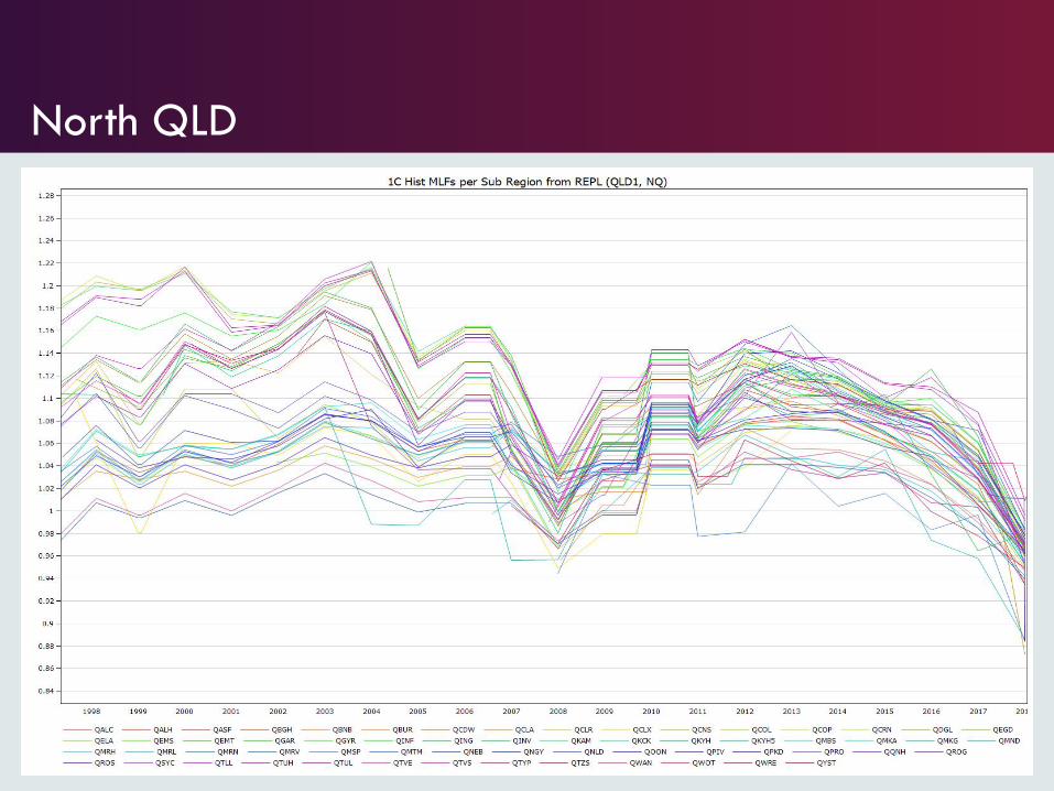
North QLD

Questions we need to answer

05/09/2018 6

1. Whether the current MLF calculations are fit for purpose.

2. Potential improvements to MLF calculations that AEMO can make through a market consultation to amend the Forward Looking Loss Factor Methodology.

3. Potential improvements to MLF calculations that require changes to the National Electricity Rules.

4. Ways AEMO can increase the transparency of the MLF calculation process and improve the ability of participants and intending participants to forecast MLFs.

What we need from these sessions

05/09/2018 7

• To affect changes in MLF process AEMO needs to amend:

• Business practices (0 – 12 months to implement changes)

• The Forward Looking Loss Factor Methodology (9 –18 months to implement changes)

• The National Electricity Rules (2 years + to implement changes)

• AEMO will be using the outcomes of this these workshops to scope and coordinate the review process.

MLF fundamentals

8

What is a Marginal Loss Factor (MLF)?

The MLF represents the marginal electrical transmission losses between a connection point and the regional reference node (RRN)

• Value assigned to a load or generator Transmission Node Identifier (TNI).

• 2018-19 calculated values range between 0.83 – 1.1

AEMO develops and publishes procedure for determining MLFs (publication process includes consultation)

• Requirement under NER 3.6.2 (Intra-regional losses)

• AEMO has little room for discretion

• Planning to open for consultation very soon – currently benchmarking international practices

9

What is a Marginal Loss Factor (MLF)?

10

Losses

MLF = 1 + ∆L/∆P

∆P +ve for load

∆P -ve for generator

RRN

Power

Station

Why have MLFs been changing?

11

Losses

0.85

0.90

0.95

1.00

1.05

2009 2010 2011 2012 2013 2014 2015 2016 2017 2018

MLF for a NQ Generator

Usage of MLFs in NEM

• To refer bid prices from connection points to the Regional Reference Node

Dispatch process

• To calculate the settlement prices for connection points

Settlement process

• For large-scale generation certificate (LGC) calculations by the CER

Renewable energy power stations

• One of the locational signals for investment decision making

Revenue/cost estimation and

budgeting

What do MLFs Do?

13

Losses

For a scheduled generator in dispatch:

Price at RRN = Bid Price/MLF

MLF = 0.9

Bid Price = $90/MWh

Price at RRN = $100/MWh

Lower MLF

Higher Price at RRN

Less likely to be dispatched

What do MLFs Do?

14

Losses

Electricity Market Settlement Income:

RRP x MLF x Measured Energy

MLF = 0.9

Measured Energy = 100 MWh

Income = $9,000

RRP = $100/MWh

Settlement revenue

Project financing

Renewable Energy Certificates (LGC)

How do MLFs effect bid stack order and settlement price?

Bid Price at the

Connection Point

MLF Bid price at Regional

Reference None (RRN)

$30/MWh 0.95 $31.58/MWh

$30/MWh 1.05 $28.57/MWh

15

Regional

Reference Price

MLF Settlement price

$50/MWh 0.95 $47.50/MWh

$50/MWh 1.05 $52.50/MWh

MLF Calculation Process

05/09/2018Example footer text 16

MLF calculation process

MLFs for the next financial year are published on 1 April

• Time consuming task, analysis starts six months before publication

• Due to time taken to confirm metering readings, data from the previous financial year is used

17

Sample

Analysis

Usage

2016-2017 2017-2018 2018-2019

Rapid changing industry (supply-demand)

• Data may not reflect operations conditions

• Mitigated by getting feedback on energy totals

• Outage information from PASA

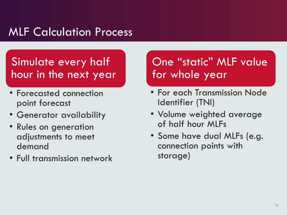
MLF Calculation Process

Simulate every half hour in the next year

• Forecasted connection point forecast

• Generator availability

• Rules on generation adjustments to meet demand

• Full transmission network

18

One “static” MLF value for whole year

• For each Transmission Node Identifier (TNI)

• Volume weighted average of half hour MLFs

• Some have dual MLFs (e.g. connection points with storage)

Data for one TNI: Time series and Scatter plot

05/09/2018Example footer text 19

𝑺𝒕𝒂𝒕𝒊𝒄 𝑴𝑳𝑭 =σ(𝑴𝑳𝑭𝒕∗ 𝑮𝒕)

σ𝑮𝒕

The MLF

Range of

marginal

losses

M

L

F

MW

M

L

F

M

W

Stakeholder Observations

Existing Generators

• Year to year volatility of MLFs

• No reliable method for long-term forecast

• Lack of process visibility

• E.g. concerns about MLF differences between adjacent nodes

New investors

• Investment risk due to volatility

• Future investment in the subregion can change the MLF of all connection points

• Renewable energy investments far away from the RRN face very low MLFs

Impact of correlation between generation

When you generate is important

• Two units with same annual energy output but different generating patterns can have a completely different MLF

• For example, if high generation when MLF was low => Low Value

Patterns are based on last year’s actuals with minimum extrapolation

• Are there better methods?

• In previous consultations different options were considered: market simulations, SRMC based dispatch etc.

• No widespread support since they do not reflect reality either

21

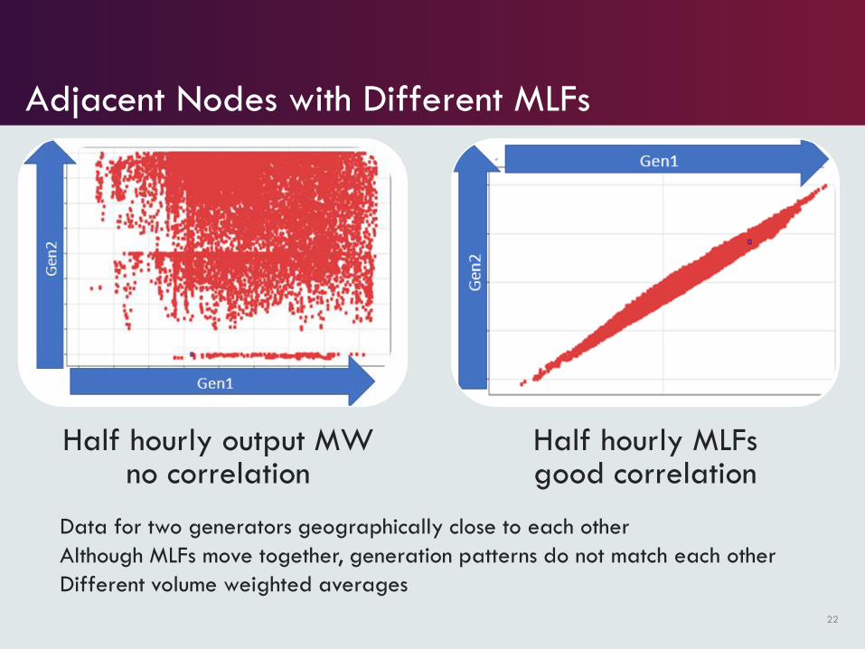
Adjacent Nodes with Different MLFs

Half hourly output MW no correlation

Half hourly MLFs good correlation

22

Data for two generators geographically close to each other

Although MLFs move together, generation patterns do not match each other

Different volume weighted averages

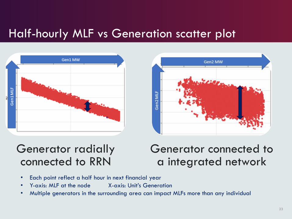
Half-hourly MLF vs Generation scatter plot

Generator radially connected to RRN

Generator connected to a integrated network

23

• Each point reflect a half hour in next financial year

• Y-axis: MLF at the node X-axis: Unit’s Generation

• Multiple generators in the surrounding area can impact MLFs more than any individual

MLF Volatility: Connectivity & Network Operation

Most generators are in integrated network

• Transmission line loading at connection point

• Extra losses when the marginal MW travelling to the RRN

• Generators in a generation rich region has a low MLF

• Generators in a load rich region has a high MLF

• Generation/consumption in the sub-region impacts all TNIs

MLFs vary from year to year due to external factors

• E.g. Generators close to an interconnector

• Low MLF in years with high import

• High MLF in years with high export

24

MLF is a forecast

As any other forecast, MLF accuracy depends on the accuracy of the input data

• Can any generator forecast their half-hourly energy output for next financial year with 10% accuracy?

• Can they forecast total annual energy GWh with 10% accuracy?

Value of forecasts can be improved by publishing sensitivity analysis

• Commercial/legal issues

• Highly time consuming process

Encourage participants to do their own sensitivity analysis

25

How are new projects factored into the calculation?

All committed projects on the cut-off day are considered

• Start days are considered

• Suitable generation or load profiles are used

• By looking at data provided by proponents

• Due diligence by AEMO

Actuals generation in the next year may vary

• Same for existing generators with short notice operational changes

• E.g. Tarong, Swanbank E, Hazelwood, Basslink outages

• AEMO uses the best information available26

Discussion

Trade-offs

• More Information vs Confidentiality

• E.g. are participants willing to share more information on upcoming projects

• Accuracy vs Certainty

• E.g. Represent actual losses or limit changes

• Dynamic vs Static values

• Simple process vs Complex & opaque simulations

05/09/2018 27

MLF potential options

05/09/2018 28

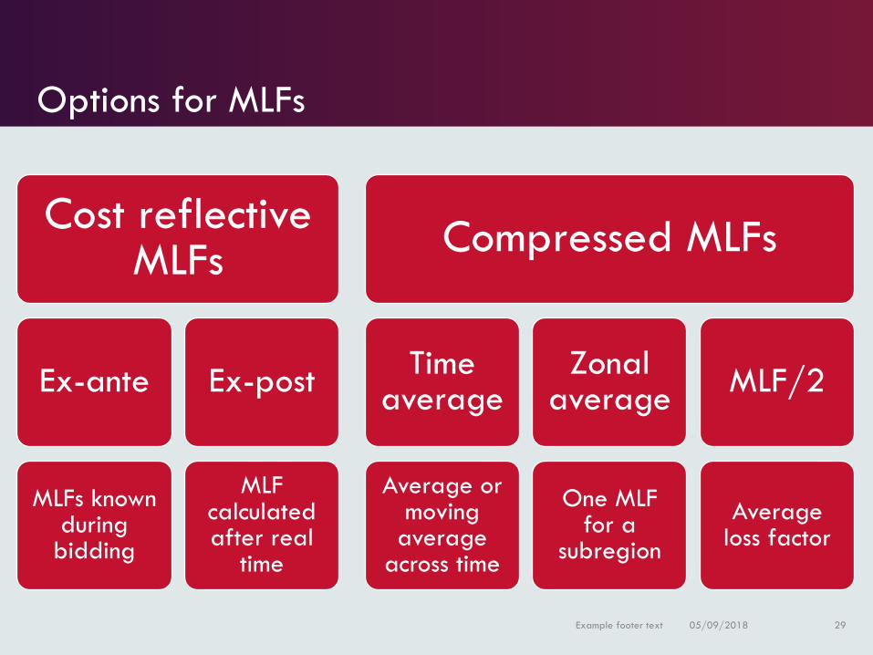
Options for MLFs

Cost reflective MLFs

Ex-ante

MLFs known during

bidding

Ex-post

MLF calculated after real

time

Compressed MLFs

Time average

Average or moving

average across time

Zonal average

One MLF for a

subregion

MLF/2

Average loss factor

05/09/2018Example footer text 29

MLF options continuum

05/09/2018Shantha R 03 August 2018 30

Certainty

Accuracy

Annual

status quo

Ex-post

Real time

forecast

Day

ahead

forecast

Monthly

peak/off-peak

Seasonal

peak/off-peak

Annual

moving avg

Grand

fathering

MLF as a

formula

Cost reflective MLFsImplementation options

05/09/2018 31

Types of options for MLF calculation

No MLFs

• Full network model

Ex-post MLFs

• Actual MLF from observed results for settlement

Ex-ante MLF

• Status quo – One per year

• Seasonal/monthly peak/off-peak day/night/weekend

• MLF as a formula (function of generation, regional demand etc)

• Dynamic forecasted MLF close to the real time

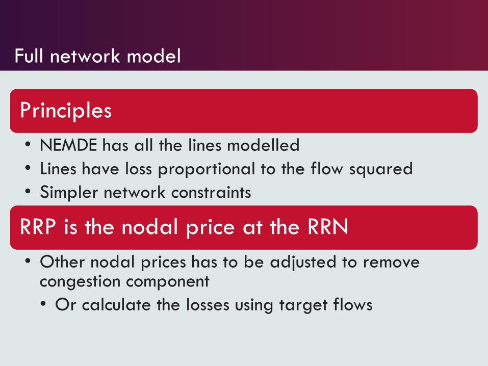
Full network model

Principles

• NEMDE has all the lines modelled

• Lines have loss proportional to the flow squared

• Simpler network constraints

RRP is the nodal price at the RRN

• Other nodal prices has to be adjusted to remove congestion component

• Or calculate the losses using target flows

Full network model

Pros

• No MLF calculation

• Simpler constraints

• Accurate modelling of network outages

Cons

• More theoretical analysis required

• Need to maintain the network model in market system

• Complex NEMDE solver required

Ex-post MLF

Principles

• Generators bid at the reference node

• Actual MLF is calculated using observed actual power flow case

Requirements

• MLF forecast provided for generators to understand limits

• State Estimator (RTNET) to calculate the MLFs or create a case to be read by other power flow software

Ex-post MLF

Pros

• Accurate MLF used for settlement

• Based on actual power flow and network outages

Cons

• Financial Volatility: Volatile prices multiplied by volatile MLFs

• Requiring risk management

• (Extreme MLFs but only apply for a short time)

• Problem during budgeting until participants develop forecasting techniques

Ex-ante MLF options

05/09/2018Example footer text 37

Status quo

Annual static MLFs

• No change in usage

Improve the calculation method

• Probabilistic calculation

Short time period MLFs

Shorter time period

• Seasonal/monthly

• peak/off-peak

• day/night/weekend

Calculation options

• In advance (April 1)

• Revise just before application time

• Forecast calculation or historical actual values

Short time period MLFs

Pros

• Calculation sample more reflective of the usage time

• If revised regularly

• Can reflect future projects accurately

• For very short term MLFs may not need forecasting

Cons

• Complexity in calculation and usage

• Volatility

• Budgeting issues

E.G. Monthly MLFs for a generator TNI

• Full month, peak and off-peak compared with annual static MLF for a TNI

0.93

0.935

0.94

0.945

0.95

0.955

0.96

0.965

0.97

1 2 3 4 5 6 7 8 9 10 11 12

MLF

Month

Monthly MLFs

Full Off-peak Peak static

MLF formula

Static number replaced by a formula

• Function of

• Measured generation

• Forecasted regional demand

• Import and interconnector flow

• Subregional supply and demand

Use the MLF calculation results

• Regression to replace volume weighted average

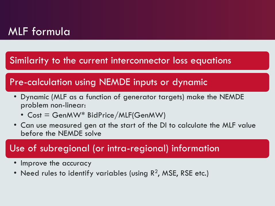
MLF formula

Similarity to the current interconnector loss equations

Pre-calculation using NEMDE inputs or dynamic

• Dynamic (MLF as a function of generator targets) make the NEMDE problem non-linear:

• Cost = GenMW* BidPrice/MLF(GenMW)

• Can use measured gen at the start of the DI to calculate the MLF value before the NEMDE solve

Use of subregional (or intra-regional) information

• Improve the accuracy

• Need rules to identify variables (using R2, MSE, RSE etc.)

MLF formulae

Pros

• Dynamic value to reflect the system conditions

• Public formula makes short-term forecasting easier

Cons

• Budgeting and forecasting issues

• Formulae based on modelling decisions

• Still may not pick some system conditions

• To get exact bids may have to allow bidding at RRN

E.g. Regression using Generation and Regional demand

MLF=

0.986973781

+ 2.18092E-06 * Gen

- 5.0877E-06 * NSWDem

Error distribution is

smaller compared to

VWA

With Gen MW With Regional Demand

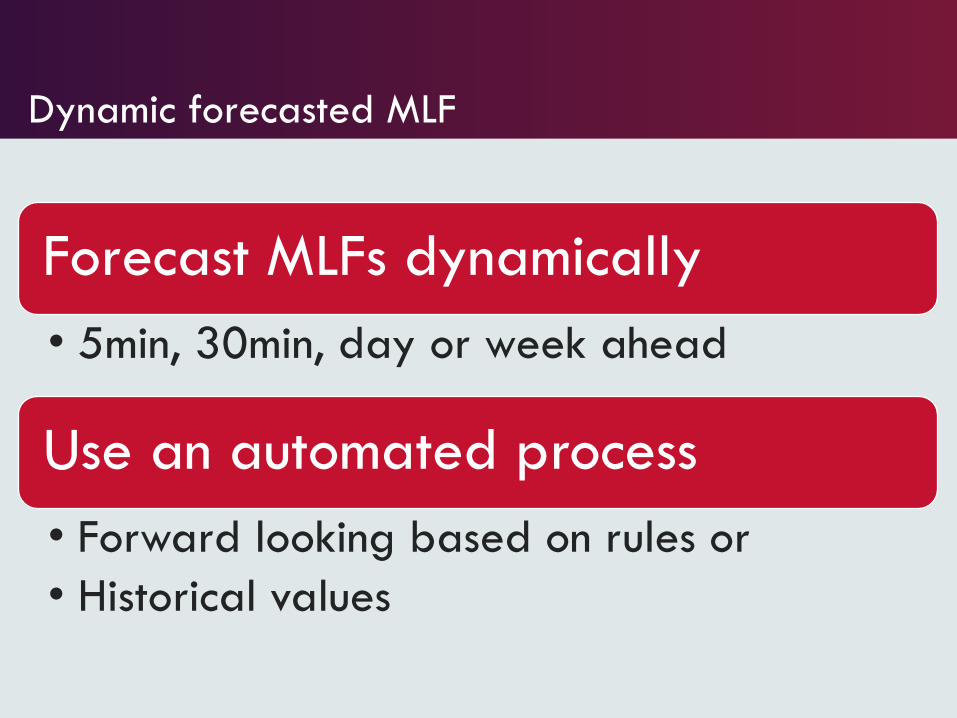
Dynamic forecasted MLF

Forecast MLFs dynamically

• 5min, 30min, day or week ahead

Use an automated process

• Forward looking based on rules or

• Historical values

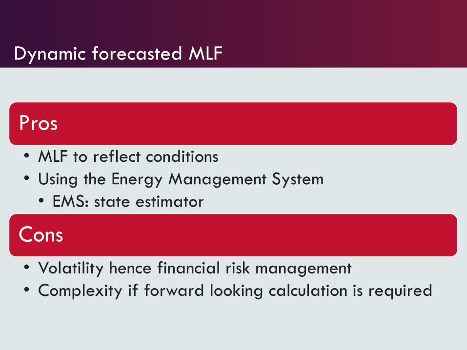
Dynamic forecasted MLF

Pros

• MLF to reflect conditions

• Using the Energy Management System

• EMS: state estimator

Cons

• Volatility hence financial risk management

• Complexity if forward looking calculation is required

Compressed Loss ModellingImplementation options

05/09/2018Example footer text 48

Types of options for compressed loss signal

Dampening the signal

• Average Loss Factors

• MLF/2

• Compressed MLFs

Grouping

• Zonal MLF

• Moving average MLFs

Average loss factors

Motivation for using ALFs

• MLFs thought to be overestimating the losses

• Only true if used as a volume multiplier

MLF is from economic theory

• Price = λ * (1 + DL/DP)

Strong arguments against ALFs

• Work by Prof Hogan, Prof Stoft etc.L

osse

s

Quantity

DL

DP

L

P

Same operating point

Marginal loss factor

MLF = 1 + DL/DP

Average loss factor

ALF = 1+ L/P

MLF/2

Variation of average loss factors

• MLF/2 = 1+ ½*DL/DP

If L = k P2

• DL/DP = 2 k P

• L/P = k P

• Under quadratic loss assumptions MLF/2 is the ALF

Same issues as in ALF

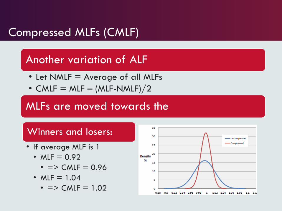
Compressed MLFs (CMLF)

Another variation of ALF

• Let NMLF = Average of all MLFs

• CMLF = MLF – (MLF-NMLF)/2

MLFs are moved towards the

Winners and losers:

• If average MLF is 1

• MLF = 0.92

• => CMLF = 0.96

• MLF = 1.04

• => CMLF = 1.02

Zonal MLFs

One MLF for a subregion

• Averaging individual MLFs

Pros

• Impact of one new addition or change is low

Cons

• Loads and generators with different load patterns get the same MLF (e.g. peakers vs baseload)

• Definition of zones can be contested

Moving averages

Aggregate over large time period

• Multi-year moving average MLFs

• Grandfathering of new investment MLFs

Winners and losers

• Each cross-subsidy has a counter party

Financial risk management options

Use intraregional residues in different manner

• Loss credit return mechanisms

• Intra-regional residue auctions

• Point to point FTRs (between RRN and Connection point)

Impact on TUoS

• Need detailed impact analysis

Increase in complexity may outweigh any benefit

55

Discussion

End of presentation

05/09/2018 56