mjh140/ChE 0401 Final Report.docx · Web viewThe data from Table 3.3d is in Figures 3.3f, 3.3g, and...
84
Batch, CSTR, and PFR Processes Final Report ChE 0401, Tuesday A-4 Matthew Ball, Ross Giglio, Krishna Gnanavel, Michael Hensler, Juliana Silva, Matthew Sompel
-
Upload
trinhthuan -
Category
Documents
-
view
214 -
download
0
Transcript of mjh140/ChE 0401 Final Report.docx · Web viewThe data from Table 3.3d is in Figures 3.3f, 3.3g, and...

Batch, CSTR, and PFR Processes
Final Report
ChE 0401, Tuesday A-4
Matthew Ball, Ross Giglio, Krishna Gnanavel,
Michael Hensler, Juliana Silva, Matthew Sompel
21 April 2017Table of Contents

1
Page1.0 Introduction and Background…………………………………………………………………3 2.0 Experimental Methodology
2.1.1 Equipment and Apparatus for Batch……………….………………………………. 62.1.2 Equipment and Apparatus for Old CSTR.…………………………………………. 62.1.3 Equipment and Apparatus for New CSTR.………………………………………….72.1.4 Equipment and Apparatus for PFR.………………………………………………... 82.2.1 Experimental Variables for Batch………………………………………………….. 82.2.2 Experimental Variables for Old CSTR…………………………………………….. 8 2.2.3 Experimental Variables for New CSTR…………………………………………… 9 2.2.4 Experimental Variables for PFR…………………………………………………… 9
3.0 Results3.1 Thermodynamic Analysis…………………………………………………………... 103.2 Batch Results…..…………………………………………………………................ 103.3 Old CSTR Results…………………………………………………………………...16 3.4 New CSTR Results…………………………………………………………………. 22 3.5 PFR Results………………………………………………………………………… 24 3.6 Statistical Analysis Results…………………………………………………………. 28
4.0 Analysis and Discussion 4.1 Batch Analysis..…………………………………………………………………….. 294.2 Old CSTR Analysis………………………………………………………………… 30 4.3 New CSTR Analysis………………………………………………………………... 33 4.4 PFR Analysis……………………………………………………………………….. 344.5 Statistical Analysis………………………………………………………………….. 364.5 Governing Principles……………………………………………………………….. 364.6 Comparison of Reactor Types……………………………………………………… 374.7 Comparison of Activation Energy Values………………………………………….. 37 4.8 Optimum Reactor Type and Operating Parameters………………………………… 37
5.0 Summary and Conclusion………………………………….………………………….......... 396.0 References………………………………………………..………………………………… 41 7.0 Appendix
7.1 Thermodynamic Calculations………………………………………………………. 42 7.2 Batch Calculations………………………………………………….......................... 42 7.3 Old CSTR Calculations………………………………………………...................... 497.4 New CSTR Calculations……………………………………………………………. 557.5 PFR Calculations……………………………………………………….................... 577.6 Statistical Analysis Calculations…………………………………………………… 62
2
Nomenclature
Symbol Term Units and Value (if applicable)
C Concentration M (mol/L)
T Temperature °C
κ Conductivity S
t Time sec
rpm Mixer Speed rpm
M Mass G
V Volume mL or L
R Rate mol/sec
k Rate Coefficient L/mol-sec
λ Specific Conductance S/m
α Conductivity temperature coefficient
mS/°C
X Conversion --
U Velocity m/s
F Volumetric Flow Rate L/sec
τ Residence Time sec
Prod Productivity M/sec
1.0 Introduction and Background

3
Saponification is a chemical process that converts esters into alcohols and carboxylic acid
salts, the primary component in soaps. In industrial settings, saponification is predominantly
used to “produce glycerol and soaps from triglycerides by reacting them with a strong alkali salt
such as sodium hydroxide (NaOH)” [1]. Often times, potassium hydroxide is used in place of
sodium hydroxide to produce more water-soluble soaps, such as those used in shaving cream [2].
Additionally, saponification is often used to study reaction kinetics in the laboratory. For
example, the saponification of ethyl acetate (EtAc) with sodium hydroxide is commonly studied
because the reactants are cheap and non-hazardous, and the reaction can be easily monitored by
measuring the conductivity of the reaction mixture [1]. In this saponification reaction, ethyl
acetate and sodium hydroxide react to form ethanol and sodium acetate (Equation 1.1).
CH3CO2C2H5 + Na+ OH- ⇔ C2H5OH + Na+ CH3CO2- (1.1)
(ethyl acetate) (sodium hydroxide) (ethanol) (sodium acetate)
Sodium hydroxide and sodium acetate are both strongly ionic, so they dissociate into their
respective ions in a polar solvent such as water [3]. Since conductivity is a function of ion
concentration, the reaction rate can be calculated from observing the change in conductivity over
time [1].
The extent to which this reaction occurs depends on parameters such as temperature,
duration of the reaction, and type of reactor. Three commonly used reactors for chemical
processes are the batch reactor, the continuously-stirred tank reactor (CSTR), and the plug flow
reactor (PFR), which are shown in Figure 1a.
Figure 1a: Diagrams of a Batch Reactor (a), CSTR (b), and PFR (c)

4
In the batch process, reactants are added to the system and uniformly mixed in a constant
volume reactor. After the reactants are added to the system, there is no flow of reactants or
products into or out of the reactor [4]. In the chemical industry batch reactors range from only a
few cm3 in volume to several stories in an industrial plant [5]. In the kettle batch process (Figure
1b), for example, fats and alkalis are melted by steam coils in a large, steel tank, or “kettle” [2].
Once melted, a salt is added to separate the glycerin from the soap. The glycerin, which settles
on the bottom of the reactor, is extracted from the reactor. Unreacted fats are saponified by
adding a caustic solution and boiling the system [2].
Figure 1b: The Kettle Batch Process [2]
The kettle batch process is used primarily by small soap manufacturers, as it typically takes four
to eleven days to complete the reaction [2]. Additionally, it takes time for different batches to be
switched out after the reaction, and the quality of multiple batches can be inconsistent [2][4]. For
this reason, leading soap manufacturers on the market make soap using continuous reactors. By
using continuous reactions, the product is continuously produced and reactants are continuously
fed, thus eliminating the need for the changing of batches. This reaction continuation also allows
operators to have greater control of the overall process quality, while also allowing for more soap
to be made in less time [2].
The two major continuous reactors are the CSTR and the PFR. In CSTR processes,
reactants are fed into the reactor and are mixed to a uniform composition by a stirring propeller.
In industrial soap-making processes using natural fat, fatty acids and glycerin are obtained from
the natural fat. Once the fatty acids and glycerin are produced, they are pumped into the CSTR
where alkali salt (such as NaOH) is added, and then the soap that forms is extracted.

5
In PFRs, material enters through one end of the tubular reactor and consistently (and
without mixing) flows through the reactor in the axial direction (Figure 1a) [5]. PFRs have many
industrial applications, such as for gas- and liquid-phase systems. PFRs are often preferred over
the use of CSTRs in positive-order, isothermal reactions because they typically run longer
without maintenance and achieve higher conversions [6].
In this experiment, batch reactors, a PFR, and CSTRs were utilized at various
temperatures and residence times to investigate the effect of reactor type on fractional
conversion, reaction rate coefficient, activation energy, and productivity [1]. There were three
batch reactors run at three different temperatures, an “old” and “new” CSTR, and a PFR. Data
was collected from two experimental runs for each type of reactor.
Each of the batch reactors was conducted at a specific temperature: room temperature,
35°C, and 45°C. The conductivity values were recorded over time and used to calculate the
conversion, reaction rate coefficient, and productivity at the three temperatures. Likewise, the
steady-state conversion, reaction rate, residence time, and productivity were calculated from the
old CSTR and PFR at room temperature, 35°C, and 45°C and at varying flow rates. Additionally,
for the new CSTR, which consisted of a single CSTR and two CSTRs in series, the volumetric
flow rates were adjusted to 2x76 mL/min, 2x51 mL/min, and 2x31 mL/min at room temperature
to examine the effect of feed rate on residence time, conversion, and productivity at steady state.
For all of these reactors except the new CSTR, the activation energy of the overall reaction was
calculated and compared to the other reactors. Statistical analysis was used to develop 90%
confidence intervals for the reaction rate coefficients at each of the temperatures and the
activation energy. Using the results from these calculations, the reactor type and parameters that
optimized the reaction were determined and analyzed.

6
2.0 Experimental Methodology
2.1.1 Equipment and Apparatus for Batch
Each of the three batch reactor systems roughly exhibited the same anatomy as shown in
Figure 2.1.1a. The only difference lies in the mechanism used to maintain proper temperature. A
water bath was used to maintain the operating temperature for the 35°C and 45°C batch reactor.
A mechanical stirrer was used to mix the reactants evenly. The conductivity and temperature
probe was also used to collect data.
Figure 2.1.1a: Batch Reactor Apparatus
2.1.2 Equipment and Apparatus for Old CSTR
The old CSTR has a relatively simple anatomy compared to that of the new CSTR. The
reactants are initially held in the chambers located to the left of the main reactor chamber shown
in Figure 2.1.2a. They are drawn out by peristaltic pumps located beneath. The pumps are
powered by the Payne power supply and push the reactants into the chamber. The conductivity
probe is also placed inside the reactor chamber to retrieve data. The temperature is controlled
through the LabView program on the computer.

7
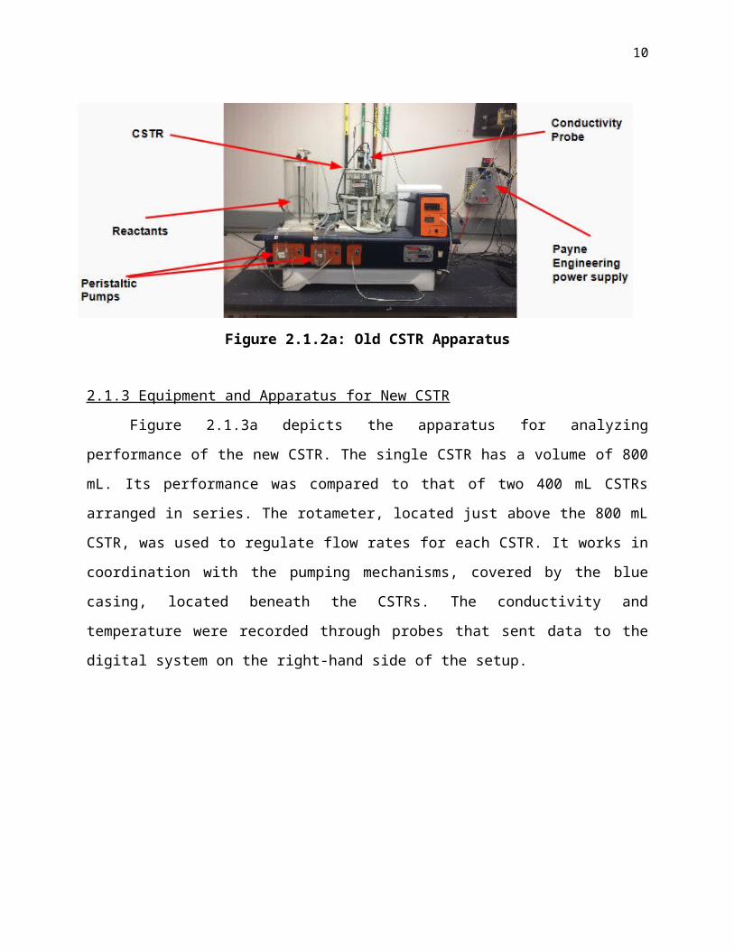
Figure 2.1.2a: Old CSTR Apparatus
2.1.3 Equipment and Apparatus for New CSTR
Figure 2.1.3a depicts the apparatus for analyzing performance of the new CSTR. The
single CSTR has a volume of 800 mL. Its performance was compared to that of two 400 mL
CSTRs arranged in series. The rotameter, located just above the 800 mL CSTR, was used to
regulate flow rates for each CSTR. It works in coordination with the pumping mechanisms,
covered by the blue casing, located beneath the CSTRs. The conductivity and temperature were
recorded through probes that sent data to the digital system on the right-hand side of the setup.
Figure 2.1.3a: New CSTR Apparatus

8
2.1.4 Equipment and Apparatus for PFR
The main power switch is the red button located on the white box to the left of the
reaction chamber. The feed pumps and reactants are located behind the panel. The tubular
reaction chamber contains reactants that convert according to their movement through the tube.
The flow is controlled by the rotameters on the panel. The temperature is controlled by a
temperature control system and monitored through a temperature probe in the tubular reactor.
Figure 2.1.4a: PFR Apparatus
2.2.1 Experimental Variables for Batch
In a 1 L batch reactor was reacted 0.1 M EtAc and 0.1 M NaOH at three different
temperatures: room temperature (23°C), 35°C, and 45°C. The water bath was heated to 35°C and
45°C in each trial by turning the temperature control knob on the apparatus. The mixer speed
was increased once these temperatures were achieved. Conductivity and temperature of the
stirred reaction were recorded for 25 min at room temperature, 20 min at 35°C, and 15 min at
45°C.
2.2.2 Experimental Variables for Old CSTR
Into a 1.67 L CSTR was fed 0.1 M NaOH and 0.1 M EtAc reactants at 30 mL/min, 50
mL/min, and 70 mL/min for the three trials. Three temperature increments were used for each
trial: room temperature, 35°C, and 45°C. To achieve 35°C and 45°C, the “set point”
temperatures were incrementally adjusted in the LabView program. Conductivity data was

9
recorded for approximately 10 min once the steady-state temperatures of 35°C and 45°C were
achieved.
2.2.3 Experimental Variables for New CSTR
Feed pumps and valves for 0.1 M NaOH and 0.1 M EtAc to the CSTR unit were opened
to recirculate the reactants in the mixture for at least a minute. The mixer speed setting for the
large, single, 0.8 L CSTR (reactor 2) was to set at 650 RPM. Using the rotameter, the flows of
NaOH and EtAc were adjusted to 76 mL/min. Conductivity and temperature were recorded every
minute until steady state was achieved. The same procedure was then conducted for the two
CSTRs in series (each 0.4 L in volume) at 375 RPM mixing speed at the same flow rates. For the
second and third sessions, the flow rates for each reactant were controlled at 51 mL/min and 31
mL/min, respectively.
2.2.4 Experimental Variables for PFR
Feed pumps of 0.1 M NaOH and 0.1 M EtAc initiated the reaction in the 1 L tubular
reaction chamber. The reaction operated at room temperature (23°C), 35°C, and 45°C for 20
min. The flow rates were adjusted to 130 mL/min, 100 mL/min, and 80 mL/min for each of the
three sessions, respectively. The conductivity and temperature were measured every minute until
steady state was achieved.
10
3.0 Results
3.1 Thermodynamic Analysis
The thermodynamic analysis was performed using parameters obtained from Courseweb,
Wikipedia, and Wired Chemist. The heat of formation of the reaction as well as the Gibbs free
energy change was calculated using these thermodynamic parameters as seen in Table 3.1a.
Using the total Gibbs free energy for the reaction, the equilibrium constant, Keq, at 35°C and
45°C was found to be 3.93x10¹¹ and 1.70x10¹¹, respectively. Using Keq, the thermodynamic
conversion values were calculated and found to be 0.999. Table 3.1a illustrates these results.
Table 3.1a: Thermodynamic Analysis
3.2 Batch Results
The batch reactor was run at three different temperatures: room temperature (23°C),
35°C, and 45°C. The graphs (Figures 3.2a, 3.2b, and 3.2c) show the conversion versus time at
the three temperatures for each lab session. In both of these graphs, the slope of the conversion
line is large for the initial couple minutes and begins to level off, signifying that the reaction is
reaching equilibrium. In these similar graphs, conversion is shown to have a large slope for the
initial three minutes and begins to decrease until the conversion settles towards an equilibrium
value. These graphs are the standard seen for batch reactors. Since there is no inlet or outlet, once
the reactants are placed in the reactor, they continue to react and eventually reach an equilibrium.

11
Figure 3.2a: Session 1 - Conversion vs. Time
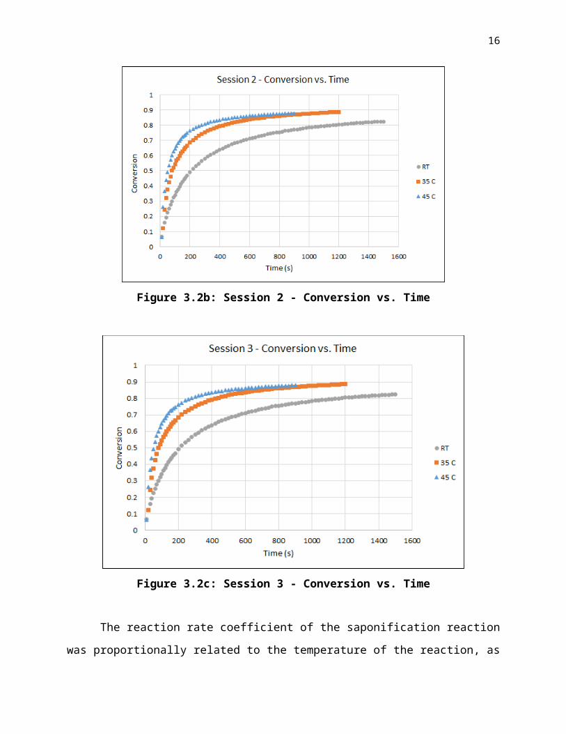
Figure 3.2b: Session 2 - Conversion vs. Time

12
Figure 3.2c: Session 3 - Conversion vs. Time
The reaction rate coefficient of the saponification reaction was proportionally related to
the temperature of the reaction, as indicated in Table 3.2a. This trend is explained by Arrhenius’
equation. Since ko , EA , and R are constant with temperature, as the (1/T) increases, the ln(k)
decreases. This relationship is graphed in Figures 3.2c and 3.2d.
Table 3.2a: Reaction Rate Coefficient (L/mol-sec)
This k value is the slope of the graph of (1/CNaOH - 1/CNaOH_0) vs. time. The time
recommended to take is the first three minutes when a sample was taken every ten seconds. This
data can be found in Figures 3.2d, 3.2e, and 3.2f. The final k values calculated for each reaction
temperature are listed in Table 3.2a.

13
Figure 3.2d: Session 1 - Reaction Rate Coefficient (mol/L-sec)
Figure 3.2e: Session 2 - Reaction Rate Coefficient (mol/L-sec)

14
Figure 3.2f: Session 3 - Reaction Rate Coefficient (mol/L-sec)
The graphs in Appendix 7.2 show a logarithmic plot of the rate coefficient vs. the inverse
of temperature (data shown in Table 3.2b). The slope of this trendline is recorded in Table 3.2c
where it is then converted to the estimated activation energy in kJ/mol.
Table 3.2b Activation Energy Estimation Data
Table 3.2c: Activation Energy Estimate (kJ/mol)
The calculated activation energies (kJ/mol) of Session 1, 2, and 3 are 38.5 kJ/mol and
37.4 and 38.5 kJ/mol, respectively.
Productivity of the saponification reaction in the batch reactors was calculated for the
three different temperatures for Sessions 1 and 2. In Figures 3.2g, 3.2h, and 3.2i, the relationship

15
shown between productivity and temperature is directly proportional because the productivity
increases as temperature of reaction is increased.
Figure 3.2g: Session 1 - Productivity (mol/L-min) vs. Temperature
Figure 3.2h: Session 2 - Productivity (mol/L-min) vs. Temperature
16
Figure 3.2i: Session 3 - Productivity (mol/L-min) vs. Temperature
The data from Table 3.2d can be found in Figures 3.2e and 3.2f. As previously stated,
productivity increases with temperature. Productivity is calculated with initial concentration and
conversion (taken to be 0.60), divided by cycle time. The final results for the productivities at
each average temperature are listed in Table 3.2d.
Table 3.2d: Productivity (mol/L-min) vs. Temperature Data
3.3 Old CSTR Results
The old CSTR was run at three temperatures: room temperature (23°C), 35°C, and 45°C
at constant flow rates. The first session tested these three temperatures at a flow rate of 50
mL/min while the second session tested these three temperatures at a flow rate of 70 mL/min.
When the reaction reached the desired temperature, the data was collected for ten minutes and

17
allowed to reach steady state. In Figures 3.3a and 3.3b, the steady state conversions are listed for
each temperature.
Figure 3.3a: Session 1 - Steady State Conversion vs. Temperature
Figure 3.3b: Session 2 - Steady State Conversion vs. Temperature

18
Figure 3.3c: Session 3 - Steady State Conversion vs. Temperature
In Table 3.3a, the reaction rate coefficient at each temperature is calculated as the average
of all of the individual k’s throughout the reaction. This total reaction rate coefficient is
dependent on temperature. Therefore, as temperature increases, there is a noticeable increase in
the k value. The final k values calculated for each reaction temperature are listed in Table 3.3a.
Table 3.3a: Reaction Rate Coefficient (L/mol-sec)
The residence time was calculated using the volume of the reactor and the flow rates of
the two reactants. Figure 3.3c is a representation of the residence time versus the flow rates.

19
Figure 3.3d: Session 1 & 2 - Residence Time vs. Flow Rate of Reactants
Residence time is the time that a reactant spends in a reactor. Therefore, flow rate of
reactants and residence times are inversely proportional. Session 1 was operated at 50 mL/min,
Session 2 was operated at a flow rate of 70 mL/min, and Session 3 was operated at a flow rate of
30 mL/min. Residence time is higher at 50 mL/min than at 70 mL/min. However, residence time
is highest at the lowest flow rate. This relationship can be seen in the mass balance.
The figures in Appendix 7.3 show a semi-logarithmic plot of the natural logarithm of the
rate coefficient versus the inverse of temperature (data shown in Table 3.3b). The slope of this
trendline is recorded in Table 3.3c where it is then converted to the estimated activation energy
in kJ/mol.
Table 3.3b: Activation Energy Estimation Data

20
Table 3.3c: Activation Energy Estimate (kJ/mol)
The calculated activation energies (kJ/mol) of Sessions 1, 2, and 3 are 33.3 kJ/mol, 35.5
kJ/mol, and 38.3 kJ/mol, respectively. Since activation energy is independent of temperature,
there is only one activation energy for each session.
Productivity of the saponification reaction in the old CSTR reactor was calculated for the
three different temperatures for Sessions 1, 2, and 3. In Figures 3.3f, 3.3g, and 3.3h, the
relationship shown between productivity and temperature is directly proportional because the
productivity increases as the temperature of reaction is increased.
Figure 3.3f: Session 1 - Productivity (mol/L-min) vs. Temperature

21
Figure 3.3g: Session 2 - Productivity (mol/L-min) vs. Temperature
Figure 3.3h: Session 3 - Productivity (mol/L-min) vs. Temperature
The data from Table 3.3d is in Figures 3.3f, 3.3g, and 3.3h. As previously mentioned,
productivity increases with temperature. Productivity is calculated with initial concentration

22
multiplied by the conversion divided by residence time. Since conversion and initial
concentration are constant, residence time is the main factor in determining the difference in
productivity between reaction temperatures. The final results for the productivities at each
average temperature are listed in Table 3.3d.
Table 3.3d: Productivity (mol/L-min) vs. Temperature Data
3.4 New CSTR Results
Table 3.4a displays the steady-state conversion values for each of the three trials.
Table 3.4a: Steady-State Conversion Values
For a single CSTR of volume 800 mL, the conversion value was 0.365 for the first trial, 0.491
for the second trial and 0.392 for the third trial. For the first CSTR reactor in series, the steady-
state conversion values were 0.286, 0.356, and 0.304 for the first, second, and third trials,
respectively. As for the second CSTR reactor in series, the first trial yielded a steady-state
conversion of 0.202, the second trial yielded a steady-state conversion of 0.294, and the third
trial yielded a steady-state conversion of 0.182. Finally, using the conversions from the first and
second CSTRs in series, the overall conversion values were calculated to be 0.430 for the first
trial, 0.545 for the second trial, and 0.431 for the third trial.
Table 3.4b shows the relationship between residence time (min) and flow rate (mL/min).

23
Table 3.4b: Residence Time versus Flow Rate
As shown in Table 3.4b, the residence times for a single CSTR and the overall residence time for
both CSTRs in series were equal. In the first trial, at a flow rate of 152 mL/min, the single and
overall residence times were 5.26 min. Similarly, the second trial yielded single CSTR and
overall residence times of 12.903 min at a flow rate of 62 mL/min. The third trial was run at a
flow rate of 51 mL/min which gave rise to a total residence time of 15.686 min.
As for the individual CSTR reactors in series, both the first and second reactors in series
produced identical residence times. For example, the first trial produced a residence time of
2.632 min for both the first and second CSTRs at a flow rate of 152 mL/min. Similarly, the
residence time for both reactors in series was 6.452 min at a volumetric flow rate of 62 mL/min.
The residence time for both reactors in series was exactly half the residence time of the single
CSTR within the same trial. This phenomenon will be further discussed in the Analysis section
(4.2 New CSTR Analysis).
The steady-state productivity values are reported in Table 3.4c in moles of NaAc/L-min.
Table 3.4c: Steady-State Productivity Values (mol/L-min)

24
During the first session, the 800 mL CSTR yielded a productivity of 0.00347 mol/L-min. The
two CSTRs in series yielded an overall productivity of 0.00409 mol/L-min. During the second
session, the single 800 mL CSTR exhibited a productivity of 0.00190 mol/L-min, while the two
CSTRs in series exhibited a productivity of 0.00211 mol/L-min. For the third trial, the single
800mL CSTR gave a productivity of 0.00125 mol/L-min while the two CSTRs in series gave a
productivity of 0.00137 mol/L-min.
3.5 PFR Results
Conversion was shown to have a linear relationship with temperature where the
conversion increased as temperature increased when the residence time of the reaction was kept
constant. This linear trend is evident in Figure 3.5a displaying conversion (%) versus
temperature (K) for two different sets of points that represent the two residence times considered
in the PFR reactor, 3.84 min and 5 min.
Figure 3.5a: Steady state conversion versus reaction temperature in a PFR
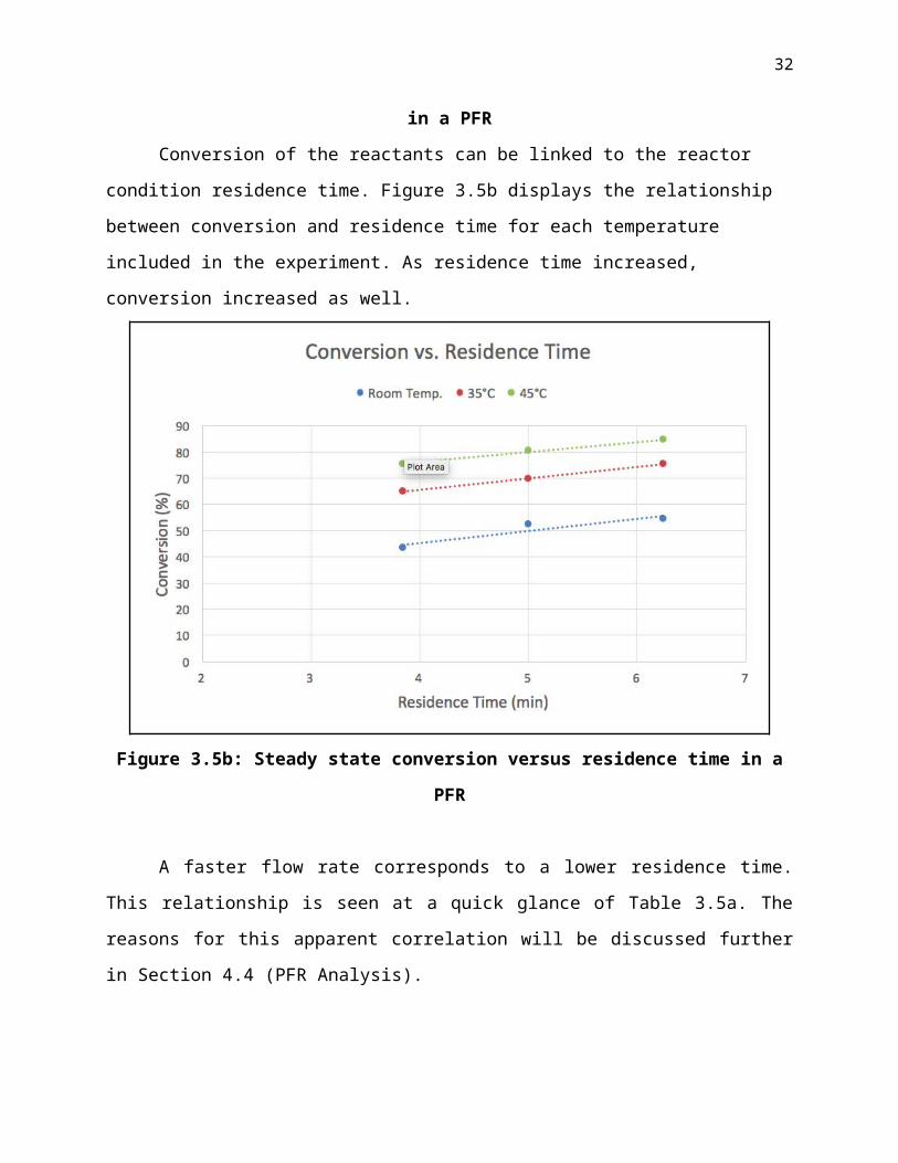
Conversion of the reactants can be linked to the reactor condition residence time. Figure
3.5b displays the relationship between conversion and residence time for each temperature
included in the experiment. As residence time increased, conversion increased as well.

25
Figure 3.5b: Steady state conversion versus residence time in a PFR
A faster flow rate corresponds to a lower residence time. This relationship is seen at a
quick glance of Table 3.5a. The reasons for this apparent correlation will be discussed further in
Section 4.4 (PFR Analysis).
Table 3.5a: Residence time versus flow rate in a PFR
The rate coefficient of the saponification reaction was related to both reactor temperature
and flow rate of the feed, as indicated in Table 3.5b. The rate coefficient (L/mol-sec) increased
when reactor temperature was increased. For example, the rate coefficient at 24°C for the 100
mL/min x 2 flow rate was calculated to be 0.073 L/mol-s as compared to 0.273 L/mol-s at 45°C
at the same flow rate.

26
Table 3.5b: Reaction rate coefficient for varying flow rates and temperatures
The graphs in Appendix 7.5 both show a logarithmic plot of the rate coefficient versus
the inverse of temperature. The plot represents a variation in the Arrhenius equation, which will
be discussed in the analysis in Section 4.
The calculated activation energies (kJ/mol) of the reactions run at three different flow
rates displayed in Table 3.5c were derived from the slopes of the respective plots of ln(k) versus
(1/T) obtained from Figures 3.5c, 3.5d, and 3.5e (Appendix 7.5). The average of the activation
energies from the three sessions was 51.17 kJ/mol.
Table 3.5c: Calculated activation energy for a saponification reaction in a PFR
Productivity of the saponification reaction in a PFR was calculated for the flow rates
studied in all three sessions. The relationship between productivity and temperature is illustrated
in Figure 3.5f, showing a higher production when the reaction was run at higher temperatures. As
for the relationship between productivity and residence time as displayed in Figure 3.5g,
productivity was lower when the residence time was higher.

27
Figure 3.5f: Productivity (mol NaAc/L-min) versus temperature (K) in a PFR
Figure 3.5g: Productivity (mol NaAc/L-min) versus residence time (min) in a PFR

28
3.6 Statistical Analysis Results
Statistical analysis of the three reactor types was performed to study the calculated
activation energy and rate coefficients at the three temperatures. Confidence intervals were
developed for these variables. The values of the statistical analysis are summarized in Table 3.6,
and sample calculations can be found in the Appendix 7.6. It is important to note that t-values
were found using corresponding degrees of freedom (n-1) of 8 and significance level α of 0.025
for a two tailed 95% confidence interval.
Table 3.6: Development of 95% Confidence Intervals from Experimental Data
Ea (kJ/mol) kRT k35°C k45°C
Batch
1st Session
2nd Session
3rd Session
38.5
37.4
38.5
0.091
0.093
0.090
0.215
0.228
0.211
0.326
0.333
0.333
CSTR
1st Session
2nd Session
3rd Session
33.3
35.5
38.3
0.098
0.088
0.088
0.161
0.154
0.156
0.233
0.235
0.238
PFR
1st Session
2nd Session
3rd Session
52.03
49.28
52.21
0.064
0.073
0.066
0.164
0.154
0.161
0.294
0.273
0.266
Mean 41.7 0.083 0.18 0.28
SD 7.35 0.012 0.030 0.042
Standard Error 2.45 0.004 0.010 0.014
t-value 2.306 2.306 2.306 2.306
95% Conf. Int. [36.04, 47.34] [0.07,0.09] [0.155, 0.202] [0.25, 0.31]

29
4.0 Analysis and Discussion
4.1 Batch Analysis
Conversion was plotted as a function of time. As seen in Figures 3.2a and 3.2b, the graph
initially increases dramatically. This increase is due to the high concentration gradient when the
liquids initially came into contact with one another. This concentration gradient is known as the
driving force, which continues to drive the reaction until equilibrium is reached. Since this
reactor is batch and not semi-batch, no additional reactant is added to the reaction. Therefore,
once equilibrium was reached, data recording was stopped. Notice that at each temperature’s
equilibrium conversion, as temperature increased, the equilibrium conversion also increased. The
data points were taken for various times. In particular, points were taken at room temperature for
25 minutes, while 35°C was only for 20 minutes, and 45°C only 15 minutes.
Realistically, each experiment would run for 25 minutes; however, this was not necessary
for the higher temperature trials. Looking at the graphs, room temperature took significantly
longer to reach equilibrium, followed by 35°C and then 45°C. Reaction rate increases with a
temperature increase. In order to prove this theory, the reaction rate coefficient was found.
The reaction rate coefficient is determined by plotting 1/Ca - 1/Cao versus time and
taking the slope of this line. In order to achieve more accurate results, the slope of the line was
taken during the first three minutes of the reaction when data readings were taken every ten
seconds. In Figures 3.2d, 3.2e and 3.2f, the k values are positive versus time. However, one must
also notice how the k values (slope) increase with temperature. This can be related back to the
reaction rate; as temperature increases, the reaction rate coefficient increases, leading to a faster
reaction rate.
After obtaining the reaction rate coefficient values for the reactions at different
temperatures, activation energy could be calculated. Activation energy can be found from a
variation of the Arrhenius equation. By plotting the three different temperature reactions on one
plot with the axes of 1/temperature versus ln(k), the slope can be calculated. By multiplying that
slope by the R value and dividing by 1000, the activation energy (kJ/mol) was found. As stated
before, there were only two activation energies: one from the first session and one from the
second. This is due to the fact that activation energy is independent of temperature. Therefore, all
three temperatures share the same activation energy because the same reaction was being
performed. The experimental values obtained for the Batch Reactor were 38.5 kJ/mol, 37.4 and

30
38.5 kJ/mol, for each session respectively. Thus, it is possible to compare the experimental data
with the literature value of 39.9 kJ/mol [9], indicating a deviation from the theoretical value of
3.51%, 6.27% and 3.51% respectively.
Plots of production versus temperature indicate how increasing temperatures affects
productivity. Productivity can be calculated from Equation 4.1a. This is similar to the equation
for the other types of reactors; however, the τcyc represents cycle time and it can be calculated
from Equation 4.1b. Charging time is defined as when the reactants are entered into the system
(FReact = 100 mL/min). Reaction time is defined as the time that has passed since the reaction has
started (X = 0.6). Discharge time is defined as the time that it takes for the products to leave the
system (FProd = 200 mL/min). A more detailed calculation can be found in the appendix.
Prod = (CNaOH_0*XNaOH) / τcyc (4.1a)
τcyc = Charging Time + Reaction Time + Discharge Time (4.1b)
The productivity was found to increase as temperature of reaction increased. This trend is
apparent in Figure 3.2g, 3.2h and 3.2i. Since initial concentration was constant throughout each
reaction, charging time and discharge time were assumed constant, and only conversion of 0.6
was considered (therefore constant), the only factor affecting productivity was reaction time.
In summary, for the batch reactor process, as temperature increases, reaction rate
coefficient and rate of reaction increase, leading to a high productivity and a constant activation
energy.
4.2 Old CSTR Analysis
The data from Table 3.3a shows that the rate coefficient increased when temperature
increased. This statement can be proved with the Arrhenius equation 4.2a, presented below. Per
the equation, when the temperature increases, the exponential term becomes less negative, since
the temperature term is part of the denominator. Thus, the rate coefficient value increases,
assuming the pre-exponential coefficient (ko) has a constant value. The highest coefficient value
comes from the highest temperature, as expected and presented in Table 3.3a.
(4.2a)

31
The conversion increases when temperature increases. It is possible to prove this concept
with the Energy Balance analysis. For a CSTR, the Energy Balance is represented by Equations
4.2b and 4.2c, assuming constant properties, single reaction, steady state and exothermic
reaction.
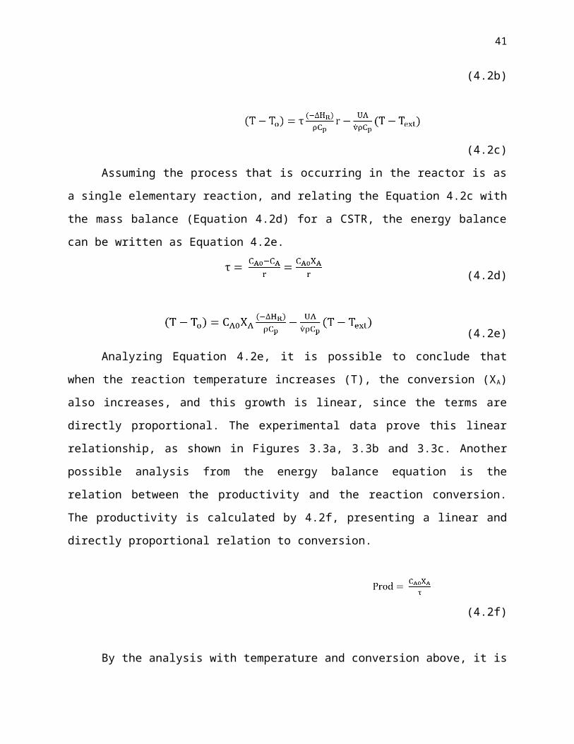
Accumulation = Input - Output + Production - Exchange (4.2b)
(4.2c)
Assuming the process that is occurring in the reactor is as a single elementary reaction,
and relating the Equation 4.2c with the mass balance (Equation 4.2d) for a CSTR, the energy
balance can be written as Equation 4.2e.
(4.2d)
(4.2e)
Analyzing Equation 4.2e, it is possible to conclude that when the reaction temperature
increases (T), the conversion (XA) also increases, and this growth is linear, since the terms are
directly proportional. The experimental data prove this linear relationship, as shown in Figures
3.3a, 3.3b and 3.3c. Another possible analysis from the energy balance equation is the relation
between the productivity and the reaction conversion. The productivity is calculated by 4.2f,
presenting a linear and directly proportional relation to conversion.
(4.2f)
By the analysis with temperature and conversion above, it is possible to conclude that the
productivity is also directly related with the temperature, i.e. when temperature increases,
productivity also increases. By the experimental data, the productivity-temperature increase is
demonstrated with Figures 3.3f, 3.3g and 3.3h.
The calculation for residence time is made by dividing the reactor volume per volumetric
flow rate. It is known that the volumetric flow rate is directly related with the molar flow rate, by
Equation 4.2h.
32
(4.2g)
(4.2h)
Replacing Equation 4.2h in the residence time calculation, it is possible to see the reverse
relation between residence time and molar flow rate.
(4.2i)
Thus, it is expected that when the flow rate increases, the residence time will decrease.
The data from Figure 3.3d accurately models what the equation predicts, with the decay of τ
when molar flow increases.
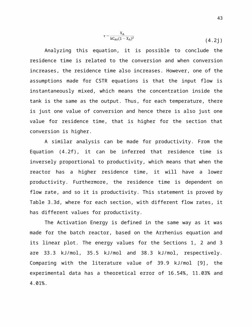
The mass balance equation for a CSTR is presented by the Equation (4.2d) and it can be
rearranged as shown in Equation (4.2j) below.
(4.2j)
Analyzing this equation, it is possible to conclude the residence time is related to the
conversion and when conversion increases, the residence time also increases. However, one of
the assumptions made for CSTR equations is that the input flow is instantaneously mixed, which
means the concentration inside the tank is the same as the output. Thus, for each temperature,
there is just one value of conversion and hence there is also just one value for residence time,
that is higher for the section that conversion is higher.
A similar analysis can be made for productivity. From the Equation (4.2f), it can be
inferred that residence time is inversely proportional to productivity, which means that when the
reactor has a higher residence time, it will have a lower productivity. Furthermore, the residence
time is dependent on flow rate, and so it is productivity. This statement is proved by Table 3.3d,
where for each section, with different flow rates, it has different values for productivity.
The Activation Energy is defined in the same way as it was made for the batch reactor,
based on the Arrhenius equation and its linear plot. The energy values for the Sections 1, 2 and 3
are 33.3 kJ/mol, 35.5 kJ/mol and 38.3 kJ/mol, respectively. Comparing with the literature value
of 39.9 kJ/mol [9], the experimental data has a theoretical error of 16.54%, 11.03% and 4.01%.

33
4.3 New CSTR Analysis
Conversion in each reactor is found by the Equation 4.3a, found below. The conversion
was dependent primarily on the conductivity readings from the probe and the initial
concentrations of reactants. The overall conversion for the two CSTRs in series was found by
Equation 4.3b below. For all the equations involving reactor 2 of the series operation, the
concentration of NaOH leaving reactor 1 was used as the initial concentration in reactor 2.
Consequently, there was also a non-zero initial concentration of NaAc that was fed into reactor
2.
XNaOH_2 = (κ - λ NaOH*CNaOH_1 - λ NaAc*CNaAc_1)/(CNaOH_1*( λ NaAc - λ NaOH)) (4.3a)
Overall: XNaOH = 1 - (1 - XNaOH_1)*(1 - XNaOH_2) (4.3b)
The operation of two CSTRs in series gave a higher conversion than operation of a single
CSTR. As seen in Table 3.4a of the Results section, the conversions for the single 800 mL
reactor were 0.365 and 0.491 for the first and second trial, respectively. Running the reactors in
series gave a higher overall conversion with the same flow rate. The overall conversion as a
result of series operation were determined to be 0.43 and 0.545 for the first and second sessions,
respectively. This trend is due to the fact that the conversion of the second reactor builds directly
on the conversion given by the first reactor. The data from the third trial supports the observed
trend from the first two trials. During the third trial, the 800 mL CSTR conversion was found to
be 0.392 while the conversion for the two CSTRs in series were found to be 0.431.
Conversion in the CSTRs generally increased as the flow rate decreased. This effect is
primarily due to the increased time that the reactants spent in the reactor (residence time). The
CSTRs were run at a faster total flow rate, 152mL/min, during the first session than that of the
second session, 62mL/min. As a result, the trend in conversion for the 800 mL CSTR from the
first to second session was an increase from 0.365 to 0.491. Similarly, the two individual CSTRs
in series increased in conversion from 0.286 to 0.355 and from 0.202 to 0.294 for reactor 1 and
reactor 2, respectively. This effect translated through to the overall conversion of the two series
CSTRs. The conversion was increased from 0.43 to 0.545 as a result of the slowed flow rate. The
conversion during the third trial should be higher than that of the second and third trial due to the
further decreased flow rate. The trend was not confirmed when a conversion of 0.392 was

34
observed for the 800 mL CSTR, and a conversion of 0.43 was observed for the series CSTRs.
The error in the trend for conversion could be a result of equilibrium limitations. The equilibrium
concentrations may have shifted due to fluctuations in temperature.
The residence time in the reactors was affected by flow rates and operation in series, as
seen in Equation 4.2g. The results in Table 3.4b show the total flow rates were held constant
throughout the trial session. The residence time for the single reactor at 152 mL/min was 5.26
minutes. The residence time of each CSTR in series was 2.63 minutes. When summing the series
operation residence times, the total time of 5.26 minutes was consistent with the single reactor.
During the second trial, the residence times were observed to be higher than that of the first trial.
The total residence time had increased from 5.26 minutes to 12.9 min. This increase was a direct
result of lowering the flow rate 152 mL/min to 62 mL/min. As discussed above, higher residence
times generally correspond to a higher conversion in a reactor. This trend was confirmed by the
third trial when the total residence time was found to be 15.6 for the third trial.
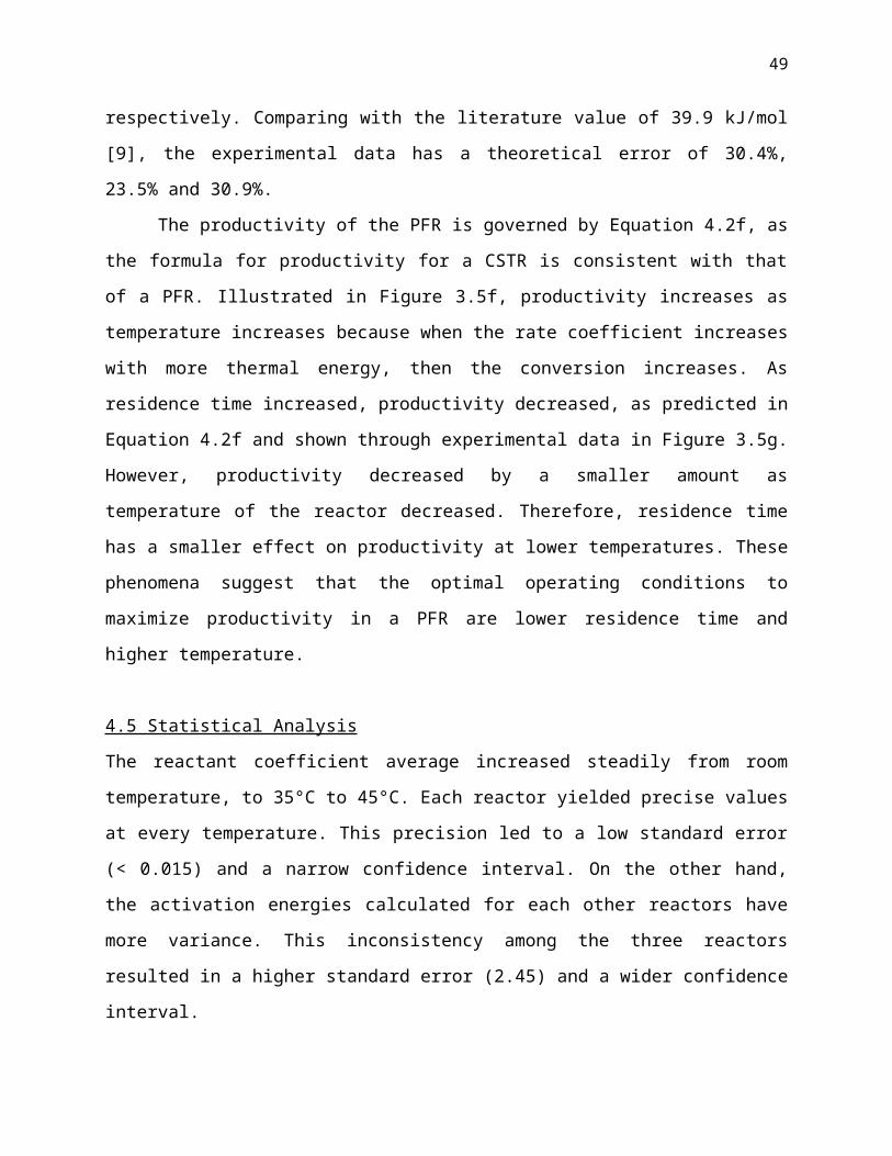
Productivity was found using Equation 4.2f. Productivity is a measure of how much
product is delivered by the reactor system. The values presented in mol NaAc/L-min are shown
in Table 3.4c of the Results section. The general trend in productivity was shown to be a
decrease with decreasing flow rate. This is intuitive because the amount of product being
delivered over a certain time is higher with a higher flow rate. As shown in Table 3.4b of the
Results section, the productivity shifted from 0.003472 mol NaAc/L-min to 0.001903 mol
NaAc/L-min from session 1 to 2, respectively. The overall productivity regarding the two series
CSTRs decreased from 0.00407 mol NaAc/L-min to 0.002113 mol NaAc/L-min from session 1
to 2, respectively. When further decreasing the flow rate to 51 mL/min, the trend was confirmed
and the productivity dropped to 0.00125 and 0.00137 for the single CSTR and series CSTRs,
respectively.
4.4 PFR Analysis
Conversion increased linearly as both reaction temperature and residence time increased.
However, in the plot of conversion vs. residence time in Figure 3.5b, the rate at which
conversion increased across temperatures decreased from a slope of 0.13 (at Room Temperature)
to 0.07 (at 45°C). The data in Table 3.5a shows that as residence time increased, flow rate
decreased. This inversely proportional relationship between residence time and flow rate is

35
evident in the definition of residence time (τ), found in 4.2g, which is the same for a PFR and
CSTR. Volume in the PFR reactor is constant at V=1L. Therefore, an increase in the residence
time results in a decrease in the flow rate.
The natural log of the reactant coefficient increased at similar, linear rates within each
flow rate for all three temperatures, evidence that k increases exponentially with respect to
temperature. This relationship is explained by Arrhenius’ Equation, found in 4.2a. As
temperature increases, the ‘exp(-E/RT)’ term increases, leading to a greater reactant coefficient
to compensate for the increase. Additionally, there is a slight increase in the reactant coefficient
values from lower residence times to higher residence times. The residence time equation and the
PFR design equation both explain this pattern. In the residence time equation found below as
Equation 4.5a as the flow rate increased, the residence time decreased which resulted in a
decrease in conversion. The rate coefficient could have increased to account for the increase in
conversion.
τ = (CNaOH_0 - CNaOH) / kCNaOH (4.5a)
In the PFR design equation (Equation 4.5b), when the flow rate was increased from 100 mL/min
to 130 mL/min, the linear velocity also increased from 0.075 m/s to 0.098 m/s, which led to an
decrease in concentration differential, or simply conversion. This decrease in conversion could
explain the apparent decrease in the rate coefficient with higher flow rates and lower residence
times.
u d/dz (CNaOH ) = (rNaOH ) (4.5b)
The sharper increase in the reactant coefficient for the higher flow rate led to a steeper slope in
the ln(k) vs. (1/T) graph (Appendix Figures 3.5c, 3.5d, and 3.5e), resulting in an activation
energy slightly greater in magnitude. For instance, the slope of the logarithmic graph of the 80
mL/min x 2 had a slope of -6258.7, compared to the 100 and 130 mL/min x 2 slopes of -5927.9
and -6282.9, respectively. This lead to varying activation energies for the same reaction type,
illustrated in Table 3.5c. Theoretically, these calculated activation energies should be equal. The
activation energy values for the sessions 1, 2 and 3 are 52.03 kJ/mol, 49.28 kJ/mol and 52.21
kJ/mol, respectively. Comparing with the literature value of 39.9 kJ/mol [9], the experimental
data has a theoretical error of 30.4%, 23.5% and 30.9%.
The productivity of the PFR is governed by Equation 4.2f, as the formula for productivity
for a CSTR is consistent with that of a PFR. Illustrated in Figure 3.5f, productivity increases as

36
temperature increases because when the rate coefficient increases with more thermal energy,
then the conversion increases. As residence time increased, productivity decreased, as predicted
in Equation 4.2f and shown through experimental data in Figure 3.5g. However, productivity
decreased by a smaller amount as temperature of the reactor decreased. Therefore, residence time
has a smaller effect on productivity at lower temperatures. These phenomena suggest that the
optimal operating conditions to maximize productivity in a PFR are lower residence time and
higher temperature.
4.5 Statistical Analysis
The reactant coefficient average increased steadily from room temperature, to 35°C to 45°C.
Each reactor yielded precise values at every temperature. This precision led to a low standard
error (< 0.015) and a narrow confidence interval. On the other hand, the activation energies
calculated for each other reactors have more variance. This inconsistency among the three
reactors resulted in a higher standard error (2.45) and a wider confidence interval.
4.6 Governing Principles
According to thermodynamic properties, the reaction is exothermic, supported by a
negative enthalpy [7]. For exothermic reactions, when the temperature increases, the reverse
direction of the reaction is favored, for an equilibrium state. However, the temperature plays a
different role in the kinetics of the reaction. A higher temperature favors the forward reaction
according to Arrhenius’ equation, where temperature is the denominator term of the negative
exponential exponent, as Equation 4.2a shows. When the rate coefficient increases, the reaction
rate also increases, raising the NaOH conversion. This can be inferred for all the reactors types,
since rate coefficient is not dependent on the reactor type. It is proved by the plot of ln(k) vs 1/T,
where all the reactors presented the same linear behavior.
The residence time is related with the flow rate as presented in Equation 4.2i. Thus, when
flow rate increases, the residence time decreases. However, with this decay in residence time, the
productivity increases, since τ is inversely proportional to productivity (Equation 4.2f). In
conclusion, the high flow rate favors the high productivity, due to the higher delivery rate of
product.

37
4.7 Comparison of Reactor Types
Conversion increased with an increase in temperature and residence time, consistent for
all reactors. The batch reactor produced the highest maximum conversion (~87%) whereas the
New CSTR produced the lowest minimum conversion (~20%). Productivity increased with an
increase in temperature and conversion. The PFR produced the highest productivity (.01 mol/L-
min) whereas the the rest of the reactors produced similar productivities. The reactor with the
highest conversion did not correlate with the reactor with the best conversion because the
residence times were different. Higher residence time lowered productivity simply because
productivity is based on time, as shown in Equation 4.2f. Higher productivity could mean either
more product made in a certain amount of time or a certain amount of product made in less time,
and this trend was apparent in all reactor types. Lastly, while the calculated activation energies
should have been similar among each reactor type, the activation energies associated with the
PFR had a larger deviation from the literature values compared to the CSTR and batch reactors.
4.8 Comparison of Activation Energy Values
Activation energy of the reaction should be constant throughout each reaction because it
is independent of the reactor type. Instead, activation energy only depends on the reaction
occurring. With that, literature shows that the estimated activation energy of this particular
saponification reaction is 39.9 ± 0.6 kJ/mol [8]. The activation energy values calculated in the
current study vary from 33.30 kJ/mol to 52.21 kJ/mol among the different reactor types. The
calculated activation energies should have been similar among each reactor type, but the
activation energies associated with the PFR had a larger deviation from the literature value. The
batch reactor modeled activation energy most accurately. While the average activation energy
obtained in this experiment was 41.17 kJ/mol, a value within 1% of the literature value, the
individual variation in activation energy can be attributed to experimental error.
4.9 Optimum Reactor Type and Operating Parameters
Determining the optimum reactor type is a major component of the design process. Since
the overall reaction is constant throughout all the reactors, the three reactor types can be
compared to determine the optimal operating conditions and the best reactor type.
To reiterate the general relationships that were analyzed within the analysis sections:

38
batch processes operate better at higher temperatures and lower cycle times while CSTR and
PFR processes operate better at higher temperatures and higher flow rates. There is a trade-off
for the CSTR and PFR processes. When the flow rates are increased, the productivity increases;
however, the residence time decreases resulting in a lower conversion.
In terms of conversion, the batch reactors had the highest (X=0.878) when the
temperature was at 45°C. In terms of productivity, the PFR reactor had the highest (Prod =
0.00981 mol/L-min) when the temperature was at 45°C and the flow rate was 260 ml/min.
Since a higher productivity is more desirable than a higher conversion for this reaction,
the PFR would be the most optimal reactor choice. The maximum conversion in the batch,
CSTR, and PFR are 0.878, 0.545, and 0.8035, respectively. The maximum productivity in the
batch, CSTR, and PFR are 0.00232, 0.00211, and 0.00981, respectively. The PFR productivity is
much greater than the batch or CSTR while not compromising too much conversion. The most
optimal reactor type would be the PFR reactor with the operating parameters of high temperature
and medium flow rate in order to compromise with parameter tradeoffs.

39
5.0 Summary and Conclusions In summary, the reaction between ethyl acetate and sodium hydroxide to form sodium
acetate and ethanol was studied using a batch reactor, an old and new CSTR, and a PFR. The
concentration of the components in the reactor were estimated by measuring the conductivity of
the solution as the reaction occurred. Therefore, conversion was measured for each experimental
trial over time in the batch reactor and at steady state in the open systems. The reactions were run
at room temperature, 35°C, and 45°C for each reactor, and the open systems were run at varying
flow rates as well. Upon collection of raw data, rate coefficient, activation energy, and
productivity were analyzed for each type of reactor in order to determine the optimal running
conditions for each type of reactor.
The batch reactor results indicate that higher reaction temperatures helped the reaction to
reach its highest conversion faster than lower temperatures. This result was due to an increase in
rate of reaction. Therefore, the batch reactor would be best utilized at higher temperatures for
this reactor to maximize conversion and productivity.
Results for both CSTR processes showed the same relationship between temperature and
conversion as the batch reactor. However, it was found that operating CSTR’s in series will give
a higher conversion than a single CSTR operation with equal volume. This result is due to the
effect of the conversion of the second CSTR building directly on the conversion of the first
CSTR. The effectiveness of the reactor is therefore compounded when the reactants pass through
two reactors instead of only one.
PFR results show similar trends to the batch reactor and the two CSTR results. The PFR
processes showed the same relationship between temperature and conversion. Furthermore, the
productivity of the PFR process increased with flow rate and temperature, but increasing flow
rate decreased conversion.
Certain results regarding the saponification reaction itself were consistent independent of
reaction type. As mentioned before, in this experiment, it was found that increasing the
temperature of the reaction increases the conversion. For the open systems, it was found that
higher flow rates decrease conversion slightly, but also increase productivity. In regards to
activation energy of the saponification reaction, the calculated activation energies varied in and
between reactors, an indication of some experimental error; however, the values remained close
to those found in the literature.

40
The results of these experiments can help decide which reactor is the best to use for this
specific saponification reaction. It is important to balance conversion and productivity when
considering the optimal conditions. Comparing the results of each reactor type, it is concluded
that if high conversion and a pure product is the goal of the reaction, then the batch reactor at
high temperatures should be used. However, the productivity of this process is low because of
the closed system nature of the process, taking a longer time to run. If a balance is needed
between conversion and productivity, then a PFR reactor at high temperatures should be used as
it gives the highest productivity with what could be an acceptable conversion. In the end, the
operator of these reactors must weigh their design specifications, cost, time, and materials to
choose the optimum reactor type and parameters for their intended use.
41
6.0 References
[1] McMahon, M. “Background and Objectives for the Research Plan Presentation”. Department
of Chemical Engineering, University of Pittsburgh. [Accessed March 1, 2017].
[2] “How Products Are Made. Advameg, Inc”. [Online]. Available:
http://www.madehow.com/Volume-2/Soap.html#ixzz41o5Jbpmn . [Accessed March 1, 2017].
[3] Kim, Y.W. and Baird, J.K. “Reaction Kinetics and Critical Phenomena: Saponification of
Ethyl Acetate at the Consolute Point of 2-Butoxyethanol + Water”. International Journal of
Thermophysics, Vol. 25, No. 4, July 2004. [Accessed March 1, 2017].
[4] Schmidt, L. D. Engineering of Chemical Reactions, 2nd Edition. Oxford University Press,
2005. [Accessed March 1, 2017].
[5] “Chemical Reactors,” The Essential Chemistry Industry Online, March 18, 2013. [Online].
Available: http://www.essentialchemicalindustry.org/processes/chemical-reactors.html.
[Accessed March 2, 2017].
[6] Wijayarathne, U. P. L. & Wasalathilake, K. C. “Simulation and Optimization of
Saponification of Ethyl Acetate in the Presence of Sodium Hydroxide in a Plug Flow Reactor
Using Aspen Plus”. International Journal of Science and Research (IJSR), Volume 3 Issue 10,
October 2014. [Accessed March 2, 2017].
[7] Wired Chemist. (2017). Retrieved March 02, 2017, from
http://www.wiredchemist.com/chemistry/data/thermodynamic-data
[8] Das, Sahoo, Magapu, & Swaminathan. “Estimation of Parameters of Arrhenius Equation for
Ethyl Acetate Saponification Reaction”. International Journal of Chemical Kinetics, Volume 43,
November 2011.
[9] Mendes, Madeira, Magalhaes & Sousa. “Chemical Reaction Engineering Lab Experiment”. Chemical Engineering Education. Universidade do Porto, 2004.

42
7.0 Appendix
7.1 Thermodynamic Calculations
1) Standard Gibb’s free energy of reactionΔGR
o = ΔGproducts - ΔGreactants
ΔGRo = (-607.7 kJ/mol + -174.1 kJ/mol) - (-380.7 kJ/mol + -332.7 kJ/mol)
ΔGRo = -68.4 kJ/mol
2) Equilibrium rate constant Keq = exp(-ΔGR
o / RT)Keq = exp(-(-68.4 kJ/mol * 1000 J/kJ) / (8.314 J/mol-K * (35°C + 273.15))Keq = 3.93E11
3) Equilibrium conversion for the reactionXeq = Keq / (1 + Keq)Xeq = 3.93E11 / (1 + 3.93E11)Xeq = 0.99
Table 3.1a: Thermodynamic Analysis
7.2 Batch Calculations
1) Temperature-adjusted lambda value for NaOHλ NaOH = (κ NaOH,std. + αNaOH,std.*(T - TNaOH,std.))/(CNaOH,std.)λ NaOH = (21.3 mS + 0.386 mS/°C*(22.3°C - 20.6°C))/(0.1 M NaOH)λ NaOH = 219.562 mS/M NaOH
43
2) Temperature-adjusted lambda value for NaAcλ NaAc = (κ NaAc,std. + αNaAc,std.*(T - TNaAc,std.))/(CNaAc,std.)λ NaAc = (6.4 mS + 0.164 mS/°C*(22.3°C - 20.6°C))/(0.1 M NaAc)λ NaAc = 66.788 mS/M NaAc
3) Steady-state conversion from conductivity for BatchXNaOH = (κ)/(CNaOH_0*( λ NaAc - λ NaOH)) - (λ NaOH)/( λ NaAc - λ NaOH)XNaOH = 4.7 mS/(0.05 M NaOH*(66.296 mS/M NaAc - 218.404 mS/M NaOH)) -
(218.404 mS/M NaOH/(66.296 mS/M NaAc - 218.404 mS/M NaOH))XNaOH = 0.8179
4) Cycle time calculationτcyc = charging time + reaction time + discharge timeτcyc = 500ml*min/100ml + 80s*min/60s + 1000ml*min/200mlτcyc = 5 + 1.33 + 5 = 11.33 min
5) Productivity calculation at steady-state for BatchProd = (CNaOH_0*XNaOH)/τcyc
Prod = (0.05 M NaOH*0.6)/11.33minProd = 0.002648 M NaOH/min
Figure 3.2a: Session 1 - Conversion vs. Time

44
Figure 3.2b: Session 2 - Conversion vs. Time
Figure 3.2c: Session 3 - Conversion vs. Time

45
Figure 3.2d: Session 1 - Activation Energy Estimate (kJ/mol)
Figure 3.2e: Session 2 - Activation Energy Estimate (kJ/mol)

46
Figure 3.2f: Session 3 - Activation Energy Estimate (kJ/mol)
Figure 3.2g: Session 1 - Reaction Rate Coefficient (mol/L-sec)

47
Figure 3.2h: Session 2 - Reaction Rate Coefficient (mol/L-sec)
Figure 3.2i: Session 3 - Reaction Rate Coefficient (mol/L-sec)

48
Figure 3.2j: Session 1 - Productivity (mol/L-min) vs. Temperature
Figure 3.2k: Session 2 - Productivity (mol/L-min) vs. Temperature
49
Figure 3.2L: Session 2 - Productivity (mol/L-min) vs. Temperature
7.3 Old CSTR Calculations
1) Temperature-adjusted lambda value for NaOHλ NaOH = (κ NaOH,std. + αNaOH,std.*(T - TNaOH,std.))/(CNaOH,std.)λ NaOH = (21.3 mS + 0.3317 mS/°C*(24.063°C - 21.2°C))/(0.1 M NaOH)λ NaOH = 222.497 mS/M NaOH
2) Temperature-adjusted lambda value for NaAcλ NaAc = (κ NaAc,std. + αNaAc,std.*(T - TNaAc,std.))/(CNaAc,std.)λ NaAc = (6.52 mS + 0.1787 mS/°C*(24.063°C - 21.2°C))/(0.1 M NaAc)λ NaAc = 70.316 mS/M NaAc
3) Steady-state conversion from conductivity for old CSTRXNaOH = (κ)/(CNaOH_0*(λ NaAc - λ NaOH)) - (λ NaOH)/( λ NaAc - λ NaOH)XNaOH = 6.359 mS/(0.05 M NaOH*(70.316 mS/M NaAc - 222.497 mS/M NaOH)) -
(222.497 mS/M NaOH/(70.316 mS/M NaAc - 222.497 mS/M NaOH))XNaOH = 0.6263
4) Residence time calculation for old CSTRτCSTR = VCSTR/FT
τCSTR = 1.67L*1000mL/1L*min/(50+50) mLτCSTR = 16.7 min
5) Rate coefficient from steady-state for old CSTR

50
k = (CNaOH_0*XNaOH)/(CNaOH_02*(1-XNaOH)²*τCSTR)
k = (0.05 M NaOH*0.6263)/((0.05 M NaOH)²*(1-0.6263)²*1002s)k = 0.08952 L/mol/s
6) Productivity calculation at steady-state for old CSTRProd = (CNaOH_0*XNaOH)/τCSTR
Prod = (0.05 M NaOH*0.6263)/16.7 minProd = 0.001875 M NaOH/min
Figure 3.3a: Session 1 - Activation Energy Estimate (kJ/mol)

51
Figure 3.3b: Session 2 - Activation Energy Estimate (kJ/mol)
Figure 3.3c: Session 3 - Activation Energy Estimate (kJ/mol)

52
Figure 3.3d: Session 1 - Steady State Conversion vs. Temperature
Figure 3.3e: Session 2 - Steady State Conversion vs. Temperature

53
Figure 3.3f: Session 3 - Steady State Conversion vs. Temperature
Figure 3.3g: Session 1, 2, & 3 - Residence Time vs. Flow Rate of Reactants

54
Figure 3.3h: Session 1 - Productivity (mol/L-min) vs. Temperature
Figure 3.3i: Session 2 - Productivity (mol/L-min) vs. Temperature

55
Figure 3.3j: Session 3 - Productivity (mol/L-min) vs. Temperature
7.4 New CSTR Calculations
1) Temperature-adjusted lambda value for NaOHλ NaOH = (κ NaOH,std. + αNaOH,std.*(T - TNaOH,std.))/(CNaOH,std.)λ NaOH = (20.2 mS + 0.4074 mS/°C*(21.3°C - 20.6°C))/(0.1 M NaOH)λ NaOH = 204.852 mS/M NaOH
2) Temperature-adjusted lambda value for NaAcλ NaAc = (κ NaAc,std. + αNaAc,std.*(T - TNaAc,std.))/(CNaAc,std.)λ NaAc = (6.05 mS + 0.1933 mS/°C*(21.3°C - 20.3°C))/(0.1 M NaAc)λ NaAc = 62.433 mS/M NaAc
3) Steady-state conversion from conductivity for a single CSTRXNaOH = (κ)/(CNaOH_0*(λ NaAc - λ NaOH)) - (λ NaOH)/( λ NaAc - λ NaOH)XNaOH = 7.64 mS/(0.05 M NaOH*(62.433 mS/M NaAc - 204.852 mS/M NaOH)) -
(204.852 mS/M NaOH/(62.433 mS/M NaAc - 204.852 mS/M NaOH))XNaOH = 0.365

56
4) Steady-state conversion from conductivity for reactors in seriesa) Reactor 1
XNaOH_1 = (κ)/(CNaOH_0*( λ NaAc - λ NaOH)) - (λ NaOH)/( λ NaAc - λ NaOH)XNaOH_1 = 8.1 mS/(0.05 M NaOH*(62.433 mS/M NaAc - 204.852 mS/M NaOH)) -
(204.852 mS/M NaOH/(62.433 mS/M NaAc - 204.852 mS/M NaOH))XNaOH_1 = 0.286
b) Reactor 2XNaOH_2 = (κ - λ NaOH*CNaOH_1 - λ NaAc*CNaAc_1)/(CNaOH_1*( λ NaAc - λ NaOH))XNaOH_2 = (7.1 mS - 204.852 mS/M NaOH*0.0357 M NaOH - 62.433 mS/M
NaAc*0.0143 M NaAc)/(0.0357 M NaOH*(62.433 mS/M NaAc - 204.852 mS/M NaOH)
XNaOH_2 = 0.202
c) OverallXNaOH = 1 - (1 - XNaOH_1)*(1 - XNaOH_2)XNaOH = 1 - (1 - 0.286)*(1 - 0.202)XNaOH = 0.430
6) Residence time calculation for a single CSTRτCSTR = VCSTR/FNaOH+NaAc
τCSTR = 0.8 L/(0.152 L/min)τCSTR = 5.263 min
7) Residence time calculation for reactors in seriesa) Reactor 1
τCSTR_1 = VCSTR_1/FNaOH+NaAc
τCSTR_1 = 0.4 L/(0.152 L/min)τCSTR_1 = 2.632 min
b) Reactor 2τCSTR_2 = VCSTR_2/FNaOH+NaAc
τCSTR_2 = 0.4 L/(0.152 L/min)τCSTR_2 = 2.632 min
c) OverallτCSTR_tot = τCSTR_1 + τCSTR_2
τCSTR_tot = 2.632 min + 2.632 minτCSTR_tot = 5.263 min

57
8) Productivity calculation at steady-state for a single CSTRProd = (CNaOH_0*XNaOH)/τCSTR
Prod = (0.05 M NaOH*0.365)/5.263 minProd = 0.00347 M NaOH/min
9) Productivity calculation at steady-state for CSTRs in seriesProd = (CNaOH_0*XNaOH)/τCSTR_tot
Prod = (0.05 M NaOH*0.430)/5.263 minProd = 0.00409 M NaOH/min
7.5 PFR Calculations
1) Temperature-adjusted lambda value for NaOHλ NaOH = (κ NaOH,std. + αNaOH,std.*(T - TNaOH,std.))/(CNaOH,std.)λ NaOH = (19.5 mS + 0.4233 mS/°C*(22°C - 21.1°C))/(0.1 M NaOH)λ NaOH = 198.8097 mS/M NaOH
2) Temperature-adjusted lambda value for NaAcλNaAc = (κ NaAc,std. + αNaAc,std.*(T - TNaAc,std.))/(CNaAc,std.)λ NaAc = (5.87 mS + 0.1585 mS/°C*(22°C - 20.5°C))/(0.1 M NaAc)λ NaAc = 61.00775 mS/M NaAc
3) Steady-state conversion from conductivity for a PFRXNaOH = (κ)/(CNaOH_0*(λ NaAc - λ NaOH)) - (λ NaOH)/( λ NaAc - λ NaOH)XNaOH = 6.79 mS/(0.05 M NaOH*(61.008 mS/M NaAc - 198.810 mS/M NaOH)) -
(198.810 mS/M NaOH/(61.009 mS/M NaAc - 198.810 mS/M NaOH))XNaOH = 0.4575
4) Rate Coefficient of the saponification reactionk = u/L * (1/CNaOH - 1/CNaOH_0)u = F/Acs = F/(π*r2)u = 0.00026 m3/min * 1min/60s / (π*(4.42E-5 m)2
u = 0.0981 m/sk = 0.0981 m/s / 1L * (1/0.02836M - 1/0.05M)k = 0.06623 L/mol-s
5) Activation energy of the saponification reaction (using the slope line from ln(k) vs. (1/T) plot)EA = -slope * REA = -(-6282.9K * 8.314 J/mol-K) * 1 kJ/1000JEA = 52.236 kJ/mol

58
6) Residence time calculation for a PFRτPFR = VPFR/FτPFR = 1 L/(260 mL/min * 1L/1000mL)τPFR = 3.8401 min
7) Productivity calculation at steady-state for a PFR
Prod = (CNaOH_0*XNaOH)/τPFR
Prod = (0.05 M NaOH*0.433)/3.84 minProd = 0.005635 M NaOH/min
Figure 3.5a: Steady state conversion versus reaction temperature in a PFR

59
Figure 3.5b: Steady state conversion versus residence time in a PFR
Figure 3.5c: Logarithmic plot of calculated rate coefficients and corresponding
temperatures used to determine activation energy for 80 mL/min x 2 flow rate

60
Figure 3.5d: Logarithmic plot of calculated rate coefficients and corresponding inverse
temperatures used to determine activation energy for 100 mL/min x 2 flow rate
Figure 3.5e: Logarithmic plot of calculated rate coefficients and corresponding inverse
temperatures used to determine activation energy for 130 mL/min x 2 flow rate

61
Figure 3.5f: Productivity (mol NaAc/L-min) versus temperature (K) in a PFR
Figure 3.5g: Productivity (mol NaAc/L-min) versus residence time (min) in a PFR

62
7.6 Statistical Analysis Calculations1) Mean of Activation Energy/Rate Coefficients
xbar = Σ(x) / number of valuesMean of Ea = (38.5 + 37.4 + 38.5 + 33.3 + … + 52.21) / 9Mean of Ea = 41.7 kJ/mol
2) Standard Deviation of a Sample SD = sqrt(variance)Variance = (1/ (n-1)) * Σ(xi - xbar)^2Variance of Ea = 1/ (9-1) * (38.5 - 41.7)^2 + … + (52.21 - 41.7)^2SD of Ea = 7.35 kJ/mol
3) Standard Error of a SampleStandard Error (SE) = SD / sqrt(n)Standard Error of Ea = 7.35 / sqrt(9)Standard Error of Ea = 2.45 kJ/mol
4) 95% Confidence Interval95% CI = xbar ± t * SE95% CI of Ea = 41.7 ± 2.306 * 2.4595% CI of Ea = [36.04, 47.34]

63
Table 3.6: Development of 95% Confidence Intervals from Experimental Data
Ea (kJ/mol) kRT k35°C k45°C
Batch
1st Session
2nd Session
3rd Session
38.5
37.4
38.5
0.091
0.093
0.090
0.215
0.228
0.211
0.326
0.333
0.333
CSTR
1st Session
2nd Session
3rd Session
33.3
35.5
38.3
0.098
0.088
0.088
0.161
0.154
0.156
0.233
0.235
0.238
PFR
1st Session
2nd Session
3rd Session
52.03
49.28
52.21
0.064
0.073
0.066
0.164
0.154
0.161
0.294
0.273
0.266
Mean 41.7 0.083 0.18 0.28
SD 7.35 0.012 0.030 0.042
Standard Error 2.45 0.004 0.010 0.014
t-value 2.306 2.306 2.306 2.306
95% Confidence Interval
[36.04, 47.34] [0.07,0.09] [0.155, 0.202] [0.25, 0.31]