arX

iv:1

804.

0459

0v1

[st

at.A

P] 2

6 M

ar 2

018

1

Mixed-Effect Modeling for Longitudinal

Prediction of Cancer Tumor

Fatemeh Nasiri and Oscar Acosta-Tamayo

Abstract

In this paper, a mixed-effect modeling scheme is proposed to construct a predictor for different

features of cancer tumor. For this purpose, a set of features is extracted from two groups of patients

with the same type of cancer but with two medical outcome: 1) survived and 2) passed away. The

goal is to build different models for the two groups, where in each group, patient-specified behavior of

individuals can be characterized. These models are then used as predictors to forecast future state of

patients with a given history or initial state. To this end, a leave-on-out cross validation method is used

to measure the prediction accuracy of each patient-specified model. Experiments show that compared

to fixed-effect modeling (regression), mixed-effect modeling has a superior performance on some of the

extracted features and similar or worse performance on the others.

Index Terms

Mixed effect model, Medical image processing, Longitudinal studies.

I. INTRODUCTION

With the increasing prevalence of the signal processing applications in the medical science,

the need for sophisticated automated processing tools is more perceived. One group of these

applications deals with different imaging systems (e.g. MRI, CT, X-ray etc.), where one can

derive useful information by studying big and diverse datasets of images taken from different

patients in different stages of a disease. However, this diversity and plurality of data is helpful

only if a proper and accurate automated tool is designed to process them.

Longitudinal study and disease tracking using medical imaging is one of the most important

and effective processes during the medical treatment. Generally speaking, this procedure usually

requires images regularly taken from patients’ organ(s) involving in disease evolution. The

information in these images hopefully guides to make better estimations regarding the future

2

state of the organs and observe the impact of different drugs in different situations. For instance,

one might be interested to discover the impact of a specific dosage of an anti-cancer drug on

the size of the tumor through the time. Therefore, the question is how to benefit from the latent

information in the temporally diverse set of medical images taken from different patients.

Statistical modeling and prediction is a practical and effective solution to address the above

problem. The main idea is to exploit the repetitive behavior of the organ/tumors in response to a

new condition (e.g. drug injection, aging etc.) and derive an accurate pattern. Like other similar

machine learning and statistical modeling problems, this task requires a diverse image dataset

with a reasonable size taken in different conditions. However, it has always been costly and more

importantly dangerous to take excessive images from individual patients to specifically model

their disease. The most feasible solution to this problem is to combine image datasets from

different patients with the same disease condition and produce a rather general model. However,

this simplification would compromise accuracy of the model due to the patient-specific behaviors

of the treatments.

In this paper, first a set of longitudinal related features from lung tumor are introduced

and extracted. Then, a non-linear mixed-effect modelization scheme is proposed to construct

predictors for each feature of each patient. The performance of these predictors are evaluated

by a cross-validation algorithm.

The rest of this paper is organized as follows. In section II, we first describe the key elements

of a mixed-effect model with some examples in the longitudinal studies. Section III explains the

main steps of the proposed mixed-effect modeling. In section IV, we discuss the performance

of the proposed mixed-effect modeling compared to fixed-effect modeling in terms of prediction

accuracy and finally, section V concludes the paper.

II. GENERAL FRAMEWORK OF A PREDICTION SYSTEM USING MIXED EFFECT MODEL

In this section, we first explain principles of the mixed-effect modeling and its necessity in

the modeling of a complex medical treatment process. Then, the main elements of a prediction

system based on the mixed-effect modeling and their different choices are discussed.

A. Principles of the mixed-effect modeling

Basically, mixed-effect modeling or mixed modeling is a flexible statistical technique to exploit

regularity in the pattern of a phenomenon which consists of both fixed and random effects [1].

3

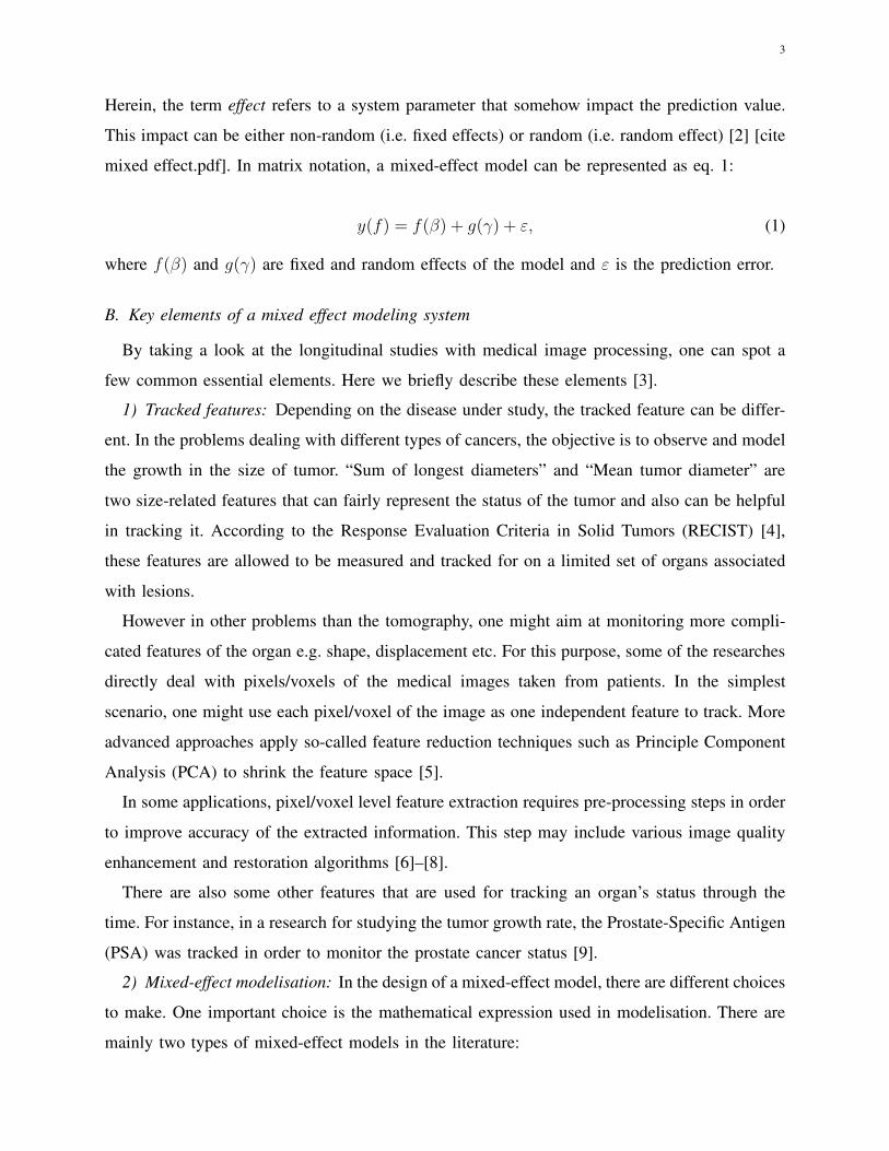
Herein, the term effect refers to a system parameter that somehow impact the prediction value.

This impact can be either non-random (i.e. fixed effects) or random (i.e. random effect) [2] [cite

mixed effect.pdf]. In matrix notation, a mixed-effect model can be represented as eq. 1:

y(f) = f(β) + g(γ) + ε, (1)

where f(β) and g(γ) are fixed and random effects of the model and ε is the prediction error.

B. Key elements of a mixed effect modeling system

By taking a look at the longitudinal studies with medical image processing, one can spot a

few common essential elements. Here we briefly describe these elements [3].

1) Tracked features: Depending on the disease under study, the tracked feature can be differ-

ent. In the problems dealing with different types of cancers, the objective is to observe and model

the growth in the size of tumor. “Sum of longest diameters” and “Mean tumor diameter” are

two size-related features that can fairly represent the status of the tumor and also can be helpful

in tracking it. According to the Response Evaluation Criteria in Solid Tumors (RECIST) [4],

these features are allowed to be measured and tracked for on a limited set of organs associated

with lesions.

However in other problems than the tomography, one might aim at monitoring more compli-

cated features of the organ e.g. shape, displacement etc. For this purpose, some of the researches

directly deal with pixels/voxels of the medical images taken from patients. In the simplest

scenario, one might use each pixel/voxel of the image as one independent feature to track. More

advanced approaches apply so-called feature reduction techniques such as Principle Component

Analysis (PCA) to shrink the feature space [5].

In some applications, pixel/voxel level feature extraction requires pre-processing steps in order

to improve accuracy of the extracted information. This step may include various image quality

enhancement and restoration algorithms [6]–[8].

There are also some other features that are used for tracking an organ’s status through the

time. For instance, in a research for studying the tumor growth rate, the Prostate-Specific Antigen

(PSA) was tracked in order to monitor the prostate cancer status [9].

2) Mixed-effect modelisation: In the design of a mixed-effect model, there are different choices

to make. One important choice is the mathematical expression used in modelisation. There are

mainly two types of mixed-effect models in the literature:

4

• Algebraic equations with the general form of:

y(t) = y0 + e−d.t + g.t. (2)

• Differential equation with the general form of:

dy

dt= y0 + e−d.t + g.t. (3)

In both equations, y is the tracked feature, t is time and d is the model parameter. In this equation,

the term exponential term of e−d.t is the random effect and the the term g.t is the fixed effect

in the model.

Once the mathematical expression is decided, one should decide about the number and the

nature of random effects of the model. For example, here is a list of some popular random

effects used in the literature of anti-cancer drug treatment:

• Drug-indudec decay of tumor

• Net growth of tumor size

• Tumor size nadir (the transition between decay and growth)

• Drug concentration

3) Response prediction: As soon as the mixed effect model is trained with the training data,

it can be used as a tool for prediction. This prediction generally includes estimation of future

state of the tracked feature. The Expectation Maximization (EM) is one of the popular methods

for addressing the response prediction problem.

III. MODELIZATION SCHEME

In this section, different steps of constructing patient-specified models are described in detail.

The following sub-sections are presented in the order of modelization procedure, starting from

raw medical images taken from patients and ending with patient-specified mixed-effect models

that are capable of prediction.

A. Feature extraction

Similar to all statistical modeling and learning tasks, an essential element of the process is

the feature selection. As explained, all features are extracted from radiology images.

5

1) Population and imaging description: The cases under this study are chosen from the

patients of the Rennes Hospital diagnosed with lung cancer. From this population, two groups

of deceased and survived patients, each with 19 persons are randomly selected.

All of the patients in the study have been through the same treatment but with different

initial states. The treatment originally includes 6 weeks of regular imaging in order to track the

situation of tumor. Each patient have been taken at least three images in this period. In other

words, there are missing entries in the input data that are supposed to be properly treated during

the modelization phase.

The first extracted feature is the volume of tumor. This criterion is measured by the number

of voxels spatially belonging to the tumor region multiplied by the size of each volume which

is defined by the imaging device. To have a precise modelization, spatial territory of each tumor

is accurately determined by a radiologist.

The second group of features relate to the tumor deformation through the time. For statistical

presentation of tumor deformation, first we have performed a registration algorithm to fit the

initial tumor shape on proper position in the next images. Then, the displacement of each voxel

is calculated and formed a 1D vector. The Jacobian matrix of this vector is calculated to provide

the second set of features. These features include mean, variance, shrewdness and kurtosis of

the Jacobian matrix. The following equation shows the calculation of the Jacobian matrix from

a vector X:

J =

[

∂f

∂x1

· · ·

∂f

∂xn

]

=

∂f1

∂x1

· · ·

∂f1

∂xn

.... . .

...

∂fm

∂x1

· · ·

∂fm

∂xn

(4)

B. Model design

Once the features data are extracted, the next step is to derive a mathematical model that

properly expresses the data properties. There are a handful of design choices in each data

modelization task that need to be carefully made with respect to the nature of data. The major

challenge in the longitudinal modelization is, as mentioned, the patient-specific behaviors.

To better understand the above challenge, here we first apply a fixed-effect model (i.e. re-

gression) on a data including patient with slightly different trends and shapes. Assume that the

6

Fig. 1. Fixed-effect modeling on a heterogeneous set of patients and its average prediction residuals for each patient.

Fig. 2. Mixed-effect modeling and its low prediction residual to address the patient-specific behaviors.

dataset consists of five patients each of which having 6 time-stamps corresponding to 6 extracted

feature. Fig. 1 shows this data with its best polynomial fitted curve in the form of θ1T2+θ2T+θ3.

As can be seen, the fitted fixed-effect model is extremely inaccurate in estimation of individual

patients’ behavior. This low performance which is reflected in relatively high residual values at

the right of Fig. 1, is due to the patient-specific trend of the data.

To address the above problem, mixed-effect modeling is used in this research. In a nutshell,

the goal is to obtain one model per patient, as shown in Fig. 2. As shown, the flexibility of

mixed-effect modeling allows us to estimate samples of each patient more accurately.

Mixed-effect (ME) models are generalizations of linear or non-linear regression models for

data that is collected and summarized in groups. ME models offer a flexible framework for

analyzing grouped data while accounting for the within group correlation often present in such

7

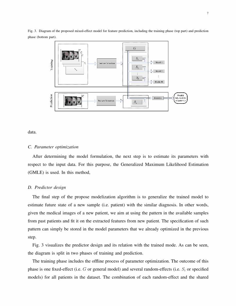
Fig. 3. Diagram of the proposed mixed-effect model for feature prediction, including the training phase (top part) and prediction

phase (bottom part).

data.

C. Parameter optimization

After determining the model formulation, the next step is to estimate its parameters with

respect to the input data. For this purpose, the Generalized Maximum Likelihood Estimation

(GMLE) is used. In this method,

D. Predictor design

The final step of the propose modelization algorithm is to generalize the trained model to

estimate future state of a new sample (i.e. patient) with the similar diagnosis. In other words,

given the medical images of a new patient, we aim at using the pattern in the available samples

from past patients and fit it on the extracted features from new patient. The specification of such

pattern can simply be stored in the model parameters that we already optimized in the previous

step.

Fig. 3 visualizes the predictor design and its relation with the trained mode. As can be seen,

the diagram is split in two phases of training and prediction.

The training phase includes the offline process of parameter optimization. The outcome of this

phase is one fixed-effect (i.e. G or general model) and several random-effects (i.e. Si or specified

models) for all patients in the dataset. The combination of each random-effect and the shared

8

fixed-effect would provide the mixed-effect model of the patient the the used random-effect

belongs to.

With the same principle, any new patient can also be modeled in the prediction phase. Once

a new patient Px arrives, its features are extracted exactly the same as the training phase. Then

the extracted features are added to the existing feature set of the past patient to update the

fixed-model G. This would also result in producing the random-effect of the new patient Sx.

Combining the updated G and Sx provides a new mixed-effect model enabling the patient Px

to predict its future state.

IV. RESULTS

In this section, the performance of the proposed mixed-effect modeling of the features is

presented. For this purpose, all the introduced features are extracted and trained by the proposed

model. The primary results of the experiments showed that only the below three features produce

relevant models:

1) Volume

2) Mean of Jacobian matrix

3) Variance of Jacobian matrix

A. One-Leave-Out cross-validation

Cross-validation is a model validation technique for statistical generalizability of a trained

model on an independent data set. In the context of this research, we intend to measure the

prediction accuracy of different models, trained by both an existing patients and the available

data from a new patient. In other words, the goal is to measure how well the trained model will

generalize and predict future state of a new patient, given his/her history that supposedly follows

the same pattern as the the existing dataset.

The main objective of all cross-validation schemes is to guarantee that the evaluation step is

performed with absolutely no bias and in a fair condition. These methods share an itertive step

that partitions the dataset into two subsets:

• Training set: this partition is used to train a new system with the same training algorithm

that we aim to validate.

9

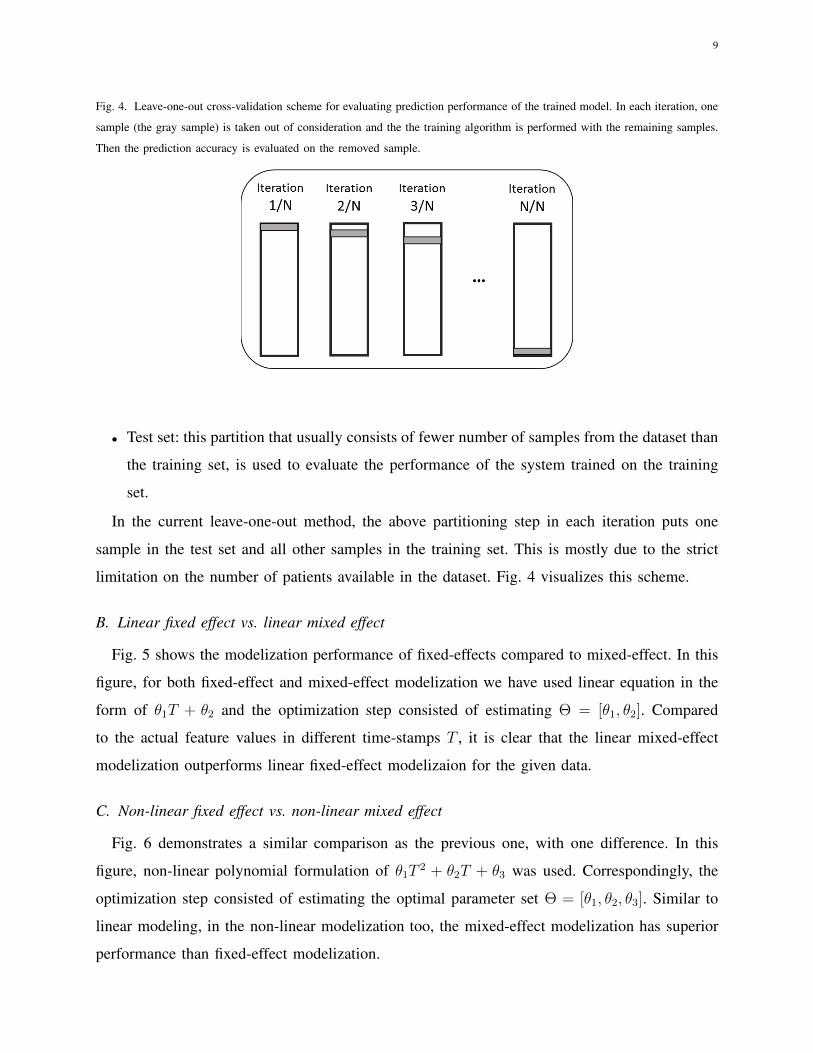
Fig. 4. Leave-one-out cross-validation scheme for evaluating prediction performance of the trained model. In each iteration, one

sample (the gray sample) is taken out of consideration and the the training algorithm is performed with the remaining samples.

Then the prediction accuracy is evaluated on the removed sample.

• Test set: this partition that usually consists of fewer number of samples from the dataset than

the training set, is used to evaluate the performance of the system trained on the training

set.

In the current leave-one-out method, the above partitioning step in each iteration puts one

sample in the test set and all other samples in the training set. This is mostly due to the strict

limitation on the number of patients available in the dataset. Fig. 4 visualizes this scheme.

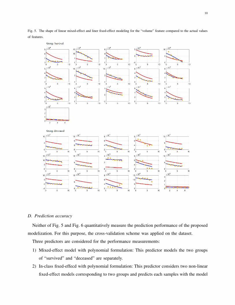
B. Linear fixed effect vs. linear mixed effect

Fig. 5 shows the modelization performance of fixed-effects compared to mixed-effect. In this

figure, for both fixed-effect and mixed-effect modelization we have used linear equation in the

form of θ1T + θ2 and the optimization step consisted of estimating Θ = [θ1, θ2]. Compared

to the actual feature values in different time-stamps T , it is clear that the linear mixed-effect

modelization outperforms linear fixed-effect modelizaion for the given data.

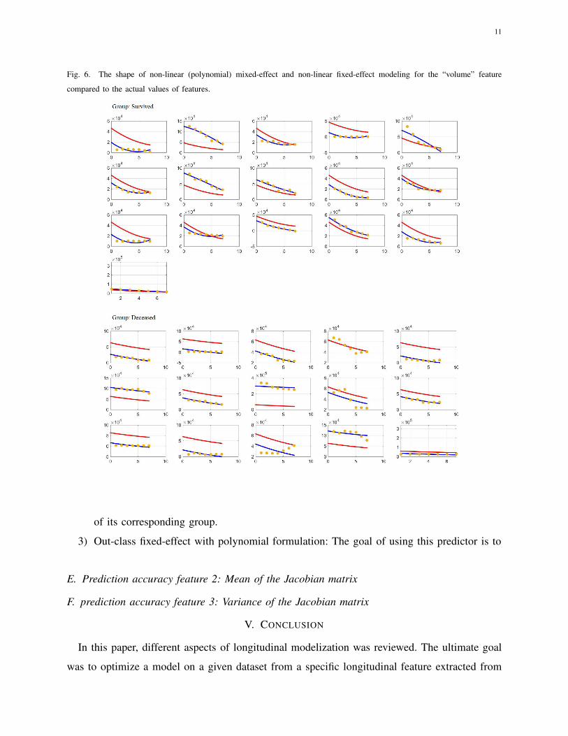
C. Non-linear fixed effect vs. non-linear mixed effect

Fig. 6 demonstrates a similar comparison as the previous one, with one difference. In this

figure, non-linear polynomial formulation of θ1T2 + θ2T + θ3 was used. Correspondingly, the

optimization step consisted of estimating the optimal parameter set Θ = [θ1, θ2, θ3]. Similar to

linear modeling, in the non-linear modelization too, the mixed-effect modelization has superior

performance than fixed-effect modelization.

10

Fig. 5. The shape of linear mixed-effect and liner fixed-effect modeling for the “volume” feature compared to the actual values

of features.

D. Prediction accuracy

Neither of Fig. 5 and Fig. 6 quantitatively measure the prediction performance of the proposed

modelization. For this purpose, the cross-validation scheme was applied on the dataset.

Three predictors are considered for the performance measurements:

1) Mixed-effect model with polynomial formulation: This predictor models the two groups

of “survived” and “deceased” are separately.

2) In-class fixed-effecd with polynomial formulation: This predictor considers two non-linear

fixed-effect models corresponding to two groups and predicts each samples with the model

11

Fig. 6. The shape of non-linear (polynomial) mixed-effect and non-linear fixed-effect modeling for the “volume” feature

compared to the actual values of features.

of its corresponding group.

3) Out-class fixed-effect with polynomial formulation: The goal of using this predictor is to

E. Prediction accuracy feature 2: Mean of the Jacobian matrix

F. prediction accuracy feature 3: Variance of the Jacobian matrix

V. CONCLUSION

In this paper, different aspects of longitudinal modelization was reviewed. The ultimate goal

was to optimize a model on a given dataset from a specific longitudinal feature extracted from

12

Fig. 7. Prediction accuracy of mixed-effect modeling vs. fixed-effect modeling for the volume feature.

Fig. 8. Prediction accuracy of mixed-effect modeling vs. fixed-effect modeling for the mean feature.

13

Fig. 9. Prediction accuracy of mixed-effect modeling vs. fixed-effect modeling for the variance feature.

past patients in a way that is capable of generalization for new patients with the same disease.

The specific disease of this study was the lung cancer and the longitudinal features were volume

of tumor and a set of features based on the deformation of tumor through the time.

The dataset that was used included two groups of patient, each having 19 members. All patients

of these two groups have suffered from lung cancer and have undergone the same treatment that

included 8 weeks of regular medical imaging. The difference between the two groups was that

the patients of the first group survived the treatment and significantly reduced their tumor size.

However, the patients of the second group did not succeed and passed away during or at the

end of this period, despite tumor size reduction.

For the feature modelization, we proposed a mixed-effect modelization scheme that allows

the modelization of each patient to benefit both from its patient-specific model and the general

patient-independent model. The experiments showed that such modelization results in much

higher prediction accuracy compared to fixed-effect modelization.

REFERENCES

[1] Fatemeh Nasiri and Oscar Acosta-Tamayo. A review of mixed-effect modeling in the longitudinal studies using medical

images of patients. arXiv preprint arXiv:1803.04241, 2018.

[2] Mary J Lindstrom and Douglas M Bates. Newtonraphson and em algorithms for linear mixed-effects models for repeated-

measures data. Journal of the American Statistical Association, 83(404):1014–1022, 1988.

14

[3] B Ribba, Nick H Holford, P Magni, I Troconiz, I Gueorguieva, P Girard, C Sarr, M Elishmereni, C Kloft, and Lena E

Friberg. A review of mixed-effects models of tumor growth and effects of anticancer drug treatment used in population

analysis. CPT: pharmacometrics & systems pharmacology, 3(5):1–10, 2014.

[4] Yoshiaki Tsuchida and Patrick Therasse. Response evaluation criteria in solid tumors (recist): new guidelines. Pediatric

Blood & Cancer, 37(1):1–3, 2001.

[5] Richard Rios, Renaud De Crevoisier, Juan D Ospina, Frederic Commandeur, Caroline Lafond, Antoine Simon, Pascal

Haigron, Jairo Espinosa, and Oscar Acosta. Population model of bladder motion and deformation based on dominant

eigenmodes and mixed-effects models in prostate cancer radiotherapy. Medical image analysis, 38:133–149, 2017.

[6] Mohsen Abdoli, Hossein Sarikhani, Mohammad Ghanbari, and Patrice Brault. Gaussian mixture model-based contrast

enhancement. IET image processing, 9(7):569–577, 2015.

[7] Aggelos K Katsaggelos. Digital image restoration. Springer Publishing Company, Incorporated, 2012.

[8] Jong-Sen Lee. Digital image enhancement and noise filtering by use of local statistics. IEEE transactions on pattern

analysis and machine intelligence, (2):165–168, 1980.

[9] Wilfred D Stein, James L Gulley, Jeff Schlom, Ravi A Madan, William Dahut, William D Figg, Yang-min Ning, Phil M

Arlen, Doug Price, Susan E Bates, et al. Tumor regression and growth rates determined in five intramural nci prostate

cancer trials: the growth rate constant as an indicator of therapeutic efficacy. Clinical Cancer Research, 2010.