Productivity Losses from Financial Frictions: Can Self ...moll/TFPFF.pdf · Productivity Losses...

American Economic Review 2014, 104(10): 3186–3221 http://dx.doi.org/10.1257/aer.104.10.3186

3186

Productivity Losses from Financial Frictions: Can Self-Financing Undo Capital Misallocation?†

By Benjamin Moll*

I develop a highly tractable general equilibrium model in which heterogeneous producers face collateral constraints, and study the effect of financial frictions on capital misallocation and aggregate productivity. My economy is isomorphic to a Solow model but with time-varying TFP. I argue that the persistence of idiosyncratic pro-ductivity shocks determines both the size of steady-state produc-tivity losses and the speed of transitions: if shocks are persistent, steady-state losses are small but transitions are slow. Even if finan-cial frictions are unimportant in the long run, they tend to matter in the short run and analyzing steady states only can be misleading. (JEL E21, E22, E23, G32, L26, O16)

Underdeveloped countries often have underdeveloped financial markets. This can lead to an inefficient allocation of capital, in turn translating into low productivity and per capita income. But available theories of this mechanism often ignore the effects of financial frictions on the accumulation of capital and wealth. Even if an entrepreneur is not able to acquire capital in the market, he might just accumulate it out of his own savings. This affects aggregates like gross domestic product (GDP), both in long-run steady state and during transitions. Existing theories which take into account accumulation are based on purely quantitative analyses, and almost none of them consider transition dynamics.1 Relative to this literature, the objec-tive of my paper is to develop a tractable dynamic general equilibrium model in which heterogeneous producers face collateral constraints, and to use it to better understand the effect of accumulation on both steady states and transition dynam-ics. I emphasize transitions in addition to steady states because they are important in their own right. They answer the basic question: if a developing country undertakes

1 A notable exception taking into account transitions is Buera and Shin (2013). See the related literature section at the end of this introduction for a more detailed discussion.

* Department of Economics, Princeton University, 106 Fisher Hall, Princeton, NJ 08544 (e-mail: [email protected]). I am extremely grateful to Rob Townsend, Fernando Alvarez, Paco Buera, Jean-Michel Lasry, Bob Lucas, and Rob Shimer for many helpful comments and encouragement. I also thank Abhijit Banerjee, Silvia Beltrametti, Roland Bénabou, Jess Benhabib, Nick Bloom, Lorenzo Caliendo, Wendy Carlin, Steve Davis, Steven Durlauf, Jeremy Fox, Veronica Guerrieri, Lars-Peter Hansen, Chang-Tai Hsieh, Erik Hurst, Oleg Itskhoki, Joe Kaboski, Anil Kashyap, Sam Kortum, David Lagakos, Guido Lorenzoni, Virgiliu Midrigan, Ezra Oberfield, Stavros Panageas, Richard Rogerson, Chad Syverson, Nicholas Trachter, Harald Uhlig, Daniel Yi Xu, Luigi Zingales, and seminar participants at the University of Chicago, Northwestern, UCLA, Berkeley, Princeton, Brown, LSE, Columbia GSB, Stanford, Yale, the 2010 Research on Money and Markets conference, the 2009 SED and the EEA-ESEM meetings, and three anonymous referees for very helpful comments. The author declares that he has no relevant or material financial interests that relate to the research described in this paper.

† Go to http://dx.doi.org/10.1257/aer.104.10.3186 to visit the article page for additional materials and author disclosure statement(s).

mailto:[email protected]

http://dx.doi.org/10.1257/aer.104.10.3186

3187Moll: Productivity losses froM financial frictionsvol. 104 no. 10

a reform, how long do its residents need to wait until they see tangible results and what factors does this depend on? Related, transitions in models of financial fric-tions have the potential to explain observed growth episodes such as the postwar miracle economies.2

Consider an entrepreneur who begins with a business idea. In order to develop his idea, he requires some capital and labor. The quality of his idea translates into his productivity in using these resources. He hires workers in a competitive labor mar-ket. Access to capital is more difficult, due to borrowing constraints; the entrepre-neur is relatively poor and hence lacks the collateral required for taking out a loan. Now consider a country with many such entrepreneurs: some poor, some rich; some with great business ideas, others with ideas not worth implementing. In a country with well-functioning credit markets, only the most productive entrepreneurs would run businesses, while unproductive entrepreneurs would lend their money to the more productive ones. In practice credit markets are imperfect so the equilibrium allocation instead has the feature that the marginal product of capital in a good entrepreneur’s operation exceeds the marginal product elsewhere. Reallocating cap-ital to him from another entrepreneur with a low marginal product would increase the country’s GDP. Failure to reallocate is therefore referred to as a misallocation of capital. Such a misallocation of capital shows up in aggregate data as low total factor productivity (TFP). Financial frictions thus have the potential to help explain differences in per capita income.3

The argument just laid out has ignored the fact that entrepreneurs can potentially overcome financial constraints through the accumulation of internal funds, and that such self-financing therefore has the potential to undo capital misallocation.4 Over time, not only an entrepreneur’s assets may change but also his productivity. It turns out that this is key for the efficacy of self-financing.

My main result is that, depending on the persistence of productivity shocks, larger steady-state productivity losses are associated with financial frictions being less important during transitions. If productivity shocks are relatively transitory, financial frictions result in large long-run productivity losses but a fast transition to steady state. Conversely, sufficiently persistent shocks imply that steady-state productivity losses are relatively small but that the transition to this steady state can take a long time. The self-financing mechanism is key to understanding this result. Consider first the steady state. If productivity shocks are sufficiently correlated over time, self-financing is an effective substitute for credit access in the long run. Conversely, if shocks are transitory, the ability of entrepreneurs to self-finance is hampered considerably. This is intuitive. While self-financing is a valid substitute to a lack of external funds, it takes time. Entrepreneurs will only have enough time to self-finance if productivity

2 This is in contrast to transitions in the neoclassical growth model which are characterized by very fast conver-gence. See Buera and Shin (2013) who make this argument by means of a quantitative theory of endogenous TFP dynamics in the presence of financial frictions.

3 I focus on the misallocation of capital rather than other resources because there is empirical evidence that this is a particularly acute problem in developing countries (Banerjee and Duflo 2005; Banerjee and Moll 2010, and the references cited therein). Restuccia and Rogerson (2008) and Hsieh and Klenow (2009) argue that resource misallocation shows up as low TFP, and Klenow and Rodríguez-Clare (1997) and Hall and Jones (1999) argue that cross-country income differences are primarily accounted for by TFP differences.

4 See Gentry and Hubbard (2004); Buera (2009); and Samphantharak and Townsend (2009) for evidence of self-financing. Quadrini (2009) argues that this contributes to high wealth concentration among entrepreneurs.

3188 THE AMERICAN ECONOMIC REVIEW OCTOBER 2014

is sufficiently persistent. The efficacy of self-financing then translates directly into long-run productivity losses from financial frictions: they are large if shocks are tran-sitory and small if they are persistent. Now consider the transition to steady state (say, after a reform that improves financial markets or removes other distortions). That transitions are slow when shocks are persistent and fast when they are transitory is the exact flip side of the steady-state result: since self-financing takes time, it results in the joint distribution of ability and wealth and therefore TFP evolving endogenously over time, which in turn prolongs the transitions of the capital stock and output. In contrast, transitory shocks imply that the transition dynamics of this joint distribution are relatively short-lived and that TFP converges quickly to its steady-state value.

The primary contribution of this paper is to make this argument by means of a tractable, dynamic theory of entrepreneurship and borrowing constraints. In the model economy, aggregate GDP can be represented as an aggregate production function. The key to this result is that individual production technologies feature constant returns to scale in capital and labor. This assumption also implies that knowledge of the share of wealth held by a given productivity type is sufficient for assessing TFP losses from financial frictions. TFP turns out to be a simple, truncated weighted average of productivities; the weights are given by the wealth shares and the truncation is increasing in the quality of credit markets.5 The assumption of individual constant returns furthermore delivers linear individual savings policies. The economy then aggregates and is simply isomorphic to a Solow model with the difference that TFP evolves endogenously over time. The evolution of TFP depends only on the evolution of wealth shares. I finally assume that the stochastic process for productivity is given by a mean-reverting diffusion. Wealth shares then obey a simple differential equation which can be characterized tightly in steady state, and solved numerically during transitions.6 Notably, this differential equation allows me to prove that there exists a unique steady-state equilibrium and that TFP losses are strictly decreasing in the persistence of shocks for a wide variety of ergodic stochas-tic processes. The representation of the joint distribution of productivity and wealth in terms of a differential equation for wealth shares and the characterization of its properties are the main methodological contributions of my paper.

Related Literature.—A large theoretical literature studies the role of financial mar-ket imperfections in economic development. Early contributions are by Banerjee and Newman (1993); Galor and Zeira (1993); Aghion and Bolton (1997); and Piketty (1997). See Banerjee and Duflo (2005) and Matsuyama (2007) for recent surveys.7 I contribute to this literature by developing a tractable theory of aggregate dynamics with forward-looking savings at the individual level.

5 Lagos (2006) provides a similar microfoundation of TFP, but in terms of labor market frictions.6 Solving for the transition dynamics in my model boils down to solving a single differential equation which is

a substantial improvement over commonly used techniques for computing transition dynamics in heterogeneous agent models with financial frictions. A typical strategy uses Monte Carlo methods: one simulates a large number of individual agents, traces the evolution of the distribution over time, and looks for an equilibrium, that is a fixed point in prices such that factor markets clear (see for example Buera, Kaboski, and Shin 2011; Buera and Shin 2013). While solving for a stationary equilibrium in this fashion is relatively straightforward, solving for transition dynamics is challenging. This is because an equilibrium is a fixed point of an entire sequence of prices (Buera and Shin 2013).

7 There is an even larger empirical literature on this topic. A well-known example is by Rajan and Zingales (1998). See Levine (2005) for a survey.


My paper is most closely related and complementary to a series of more recent, quantitative papers relating financial frictions to aggregate productivity (Jeong and Townsend 2007; Quintin 2008; Amaral and Quintin 2010; Buera, Kaboski, and Shin 2011; Buera and Shin 2013; Caselli and Gennaioli 2013; Midrigan and Xu 2014). With the exception of Jeong and Townsend (2007) and Buera and Shin (2013), all of these papers focus on steady states,8 and all of them feature purely quantitative exercises. As a result, relatively little is known about transition dynamics and how various aspects of the environment affect the papers’ quantitative results. In con-trast, my paper offers a tractable theory of aggregate dynamics that I use to highlight the role played by the persistence of productivity shocks in determining the size of productivity losses from financial frictions, particularly the differential implications of persistence for both steady states and transition dynamics. A finding with poten-tially important implications for quantitative studies is that steady-state TFP is not only increasing in persistence but also turns out to be a steep function of persistence for high values of the latter, meaning that similar values of persistence may be quite far apart from each other in terms of TFP losses.9

Caselli and Gennaioli (2013) provide one of the first frameworks linking financial market imperfections to capital misallocation and cross-country TFP differences. They are also the first to articulate the intuition that steady-state TFP losses are decreasing in the persistence of productivity shocks.10 My paper differs from theirs both in the framework used to make this point and the nature of the persistence result. Caselli and Gennaioli study a dynastic economy in which individuals live for one period and bequeath an exogenous fraction of their wealth to their offspring (due to a warm glow motive). Productivity shocks take the form of talent draws at birth and consequently their notion of persistence is the heritability of talent across generations. In my framework, in contrast, entrepreneurs are infinitely lived and adjust their assets in the face of new productivity shocks and not just once per gen-eration.11 Given their interest in understanding the prevalence of dynastic manage-ment in poor countries, Caselli and Gennaioli’s setup features a market for control in which untalented heirs can potentially sell their firms to talented outsiders. In con-trast, I abstract from such a market for simplicity. These differences in framework

8 My paper is complementary to Buera and Shin (2013), but differs along two dimensions. First, my model is highly tractable, whereas their analysis is purely numerical, though in a somewhat more general framework with decreasing returns and occupational choice. Second, they do not discuss the sensitivity of their results with respect to the persistence of shocks. In a follow-up paper, Buera and Shin (2011) do examine the sensitivity of steady-state productivity (and also welfare) losses to persistence, but not how it affects the speed of or productivity losses during transitions. My paper also differs from Jeong and Townsend (2007) in various respects. Among other differences, their model features overlapping generations of two-period-lived individuals. Hence individuals are constrained to adjust their savings only once during their entire lifetime, which may be problematic for quantita-tive results if the self-financing mechanism described earlier in this introduction is potent in reality. See Giné and Townsend (2004); Jeong and Townsend (2008); and Townsend (2010) for more on transition dynamics. See Erosa and Hidalgo-Cabrillana (2008) for another tractable model of finance and TFP with overlapping generations.

9 As I discuss in more detail in the paper, the steepness of TFP for high values of persistence potentially allows for a reconciliation of some of the very different quantitative results in the literature (Buera, Kaboski, and Shin 2011; Midrigan and Xu 2014).

10 Related, Bénabou (2002, footnote 7) notes that in a model of human capital accumulation, the persistence of ability or productivity shocks matters because it governs the intergenerational persistence of human wealth and hence welfare. Gourio (2008) shows that also the effect of adjustment costs depends crucially on persistence. None of these papers analyze the effect of persistence on transitions as in the present paper.

11 My entrepreneurs are also forward-looking and optimally split their profits between consumption and savings. Among other things, this allows me to extend the model so as to examine the effect of variations in entrepreneurs’ risk aversion on steady-state TFP losses and capital-to-output ratios.


mean that the questions the two frameworks are most suited for also differ. Caselli and Gennaioli’s setup is clearly more useful for understanding dynastic manage-ment, but mine is for example more suited for studying transition dynamics follow-ing reforms.12 Apart from these differences in framework, I add to their persistence result in three respects. First, their steady-state result is numerical and for a par-ticular stochastic process with two productivity types while I prove that TFP losses are strictly decreasing in the persistence of shocks, and that this result holds for a wide variety of stochastic processes with a continuum of productivity types. Second, I add to this steady-state result by examining the effect of persistence on transition dynamics and show that the case with small steady-state TFP losses is also the one with slow transitions. Third, I analyze the effect of persistence on overall welfare in the economy, thereby balancing its effect on steady states and transition dynamics.

Technologies in my framework are assumed to be concave, and I do not con-sider the effect of nonconvexities in production (for example, fixed costs or other indivisibilities) on the self-financing process. The idea that nonconvexities may lead financial frictions to have large effects on the macroeconomy goes back to Dasgupta and Ray (1986); Banerjee and Newman (1993); Galor and Zeira (1993); and Ljungqvist (1993), and the same is true in the context of my paper.13 The reason is that nonconvexities may disrupt the self-financing mechanism emphasized in my paper: an entrepreneur who is too far below a particular nonconvexity would choose not to save up even if high returns awaited at high asset levels.14 To the extent that nonconvexities in production are important in reality, productivity losses from finan-cial frictions in my framework should be viewed as a lower bound.

To deliver my model’s tractability, I build on work by Angeletos (2007) and Kiyotaki and Moore (2012). Their insight is that heterogeneous agent economies remain tractable if individual production functions feature constant returns to scale because then individual policy rules are linear in individual wealth. In contrast to the present paper, Angeletos focuses on the role of incomplete markets à la Bewley and does not examine credit constraints (only the so-called natural borrowing limit). Kiyotaki and Moore analyze a similar setup with borrowing constraints but focus on aggregate fluctuations. Both papers assume that productivity shocks are i.i.d. over time, an assumption I dispense with. Note that this is not a minor difference: allowing for persistent shocks is on one hand considerably more challenging tech-nically, but also changes results dramatically. Assuming i.i.d. shocks in my model would lead one to miss most interesting transition dynamics. Persistent shocks are,

12 Caselli and Gennaioli’s framework is ill-suited to study transition dynamics because their assumption that entrepreneurs adjust assets only once per generation implies that transitions will necessarily be slow.

13 See also Mookherjee and Ray (2003); Banerjee and Duflo (2005); and Banerjee and Moll (2010); Buera, Kaboski, and Shin (2011); Midrigan and Xu (2014) for recent theoretical and quantitative analyses of this idea. A concave technology is of course also the crucial assumption in the neoclassical growth model. Indeed, convergence in the neoclassical growth model—in which the economy as a whole has no access to capital markets whatsoever—can be viewed as stating that self-financing completely undoes all capital misallocation.

14 In the absence of random shocks, nonconvexities would result in poverty traps at the individual level. The same may no longer be true when entrepreneurs face productivity shocks as in the present paper. However, nonconvexities would still hamper entrepreneurs’ ability to self-finance considerably. Note the differential interaction of shocks with the convex and nonconvex parts of the technology: shocks hamper self-financing when technology is convex, but aid it when it is nonconvex.


of course, also the empirically relevant assumption.15 Buera and Moll (2012) use the framework of the present paper, but to study business cycle fluctuations driven by fluctuations in financial frictions rather than cross-country income differenc-es.16 Finally, I contribute to broader work on the macroeconomic effects of micro-distortions (Restuccia and Rogerson 2008; Hsieh and Klenow 2009; Bartelsman, Haltiwanger, and Scarpetta 2013). Hsieh and Klenow (2009) in particular argue that misallocation of both capital and labor substantially lowers aggregate TFP in India and China. Their analysis makes use of abstract wedges between marginal products. In contrast, I formally model one reason for such misallocation: financial frictions resulting in a misallocation of capital.

After developing my model (Section I), I demonstrate the importance of the per-sistence of productivity shocks (Section II), and discuss to what extent some of my modeling choices can be relaxed (Section III). Section IV is a conclusion.

I. Model

A. Preferences and Technology

Time is continuous. There is a continuum of entrepreneurs that are indexed by their productivity z and their wealth a. Productivity z follows some Markov process (the exact process is irrelevant for now).17 I assume a law of large numbers so the share of entrepreneurs experiencing any particular sequence of shocks is determin-istic. At each point in time t, the state of the economy is then the joint distribution g t (a, z). The corresponding marginal distributions are denoted by φ t (a) and ψ t (z). Entrepreneurs have preferences

(1) 피 0 ∫ 0 ∞ e −ρt log c(t) dt.

Each entrepreneur owns a private firm which uses k units of capital and ℓ units of labor to produce

(2) y = f (z, k, ℓ) = (zk ) α ℓ 1−α

units of output, where α ∈ (0, 1). Capital depreciates at the rate δ. There is also a mass L of workers. Each worker is endowed with one efficiency unit of labor which he supplies inelastically. Workers have the same preferences as (1) with the

15 Kiyotaki (1998) does allow for persistent shocks but in a considerably less general way than in my paper (a two-state Markov chain). Other papers exploiting linear savings policy rules in environments with heterogeneous agents are Banerjee and Newman (2003); Azariadis and Kaas (2012); Kocherlakota (2009); and Krebs (2003). Bénabou (2002) shows that even with nonconstant returns, it is possible to retain tractability in heterogeneous agent economies by combining log linear individual technologies with log normally distributed shocks, thereby allowing him to study issues of redistribution. In my model with constant returns to scale, there is no motive for progressive redistribution (except possibly the provision of insurance).

16 In particular, they study in more detail one implication of my framework, namely that financial frictions have no direct effect on aggregate savings and instead affect savings indirectly through TFP, and relate this to the litera-ture using wedges to summarize business cycles.

17 Here, productivity is a stand-in term for a variety of factors such as entrepreneurial ability, an idea for a new product, an investment opportunity, but also demand-side factors such as idiosyncratic demand shocks.


exception that they face no uncertainty so the expectation is redundant. The assump-tion of logarithmic utility makes analytical characterization easier but can be gener-alized to constant relative risk aversion (CRRA) utility at the expense of some extra notation. See Section III that discusses this extension.

B. Budgets

Entrepreneurs hire workers in a competitive labor market at a wage w(t). They also rent capital from other entrepreneurs in a competitive capital rental market at a rental rate R(t). This rental rate equals the user cost of capital: that is R(t) = r(t) + δ, where r(t) is the interest rate and δ the depreciation rate. An entrepreneurs’ wealth, denoted by a(t), then evolves according to

(3) a = f (z, k, ℓ) − wℓ − (r + δ)k + ra − c.

Savings a equal profits—output minus payments to labor and capital—plus interest income minus consumption. The setup with a rental market is chosen solely for sim-plicity. I show in Appendix C that it is equivalent to a setup in which entrepreneurs own and accumulate capital k and can trade in a risk-free bond.

Entrepreneurs face collateral constraints

(4) k ≤ λa, λ ≥ 1.

This formulation of capital market imperfections is analytically convenient. Moreover, by placing a restriction on an entrepreneur’s leverage ratio k/a, it cap-tures the common intuition that the amount of capital available to an entrepreneur is limited by his personal assets. Different underlying frictions can give rise to such collateral constraints.18 Finally, note that by varying λ, I can trace out all degrees of efficiency of capital markets; λ = ∞ corresponds to a perfect capital market, and λ = 1 to the case where it is completely shut down. λ therefore captures the degree of financial development, and one can give it an institutional interpretation. The form of the constraint (4) is more restrictive than required to derive my results, a point I discuss in more detail in online Appendix D. I show there that all my theoretical results go through with slight modification for the case where the maxi-mum leverage ratio λ is an arbitrary function of productivity so that (4) becomes k ≤ λ(z) a. The maximum leverage ratio may also depend on the interest rate and wages, calendar time, and other aggregate variables. What is crucial is that the col-lateral constraint is linear in wealth. Entrepreneurs are allowed to hold negative wealth, but I show below that they never find it optimal to do so.

18 For example, the constraint can be motivated as arising from a limited enforcement problem. Consider an entrepreneur with wealth a who rents k units of capital. The entrepreneur can steal a fraction 1/λ of rented capital. As a punishment, he would lose his wealth. In equilibrium, the financial intermediary will rent capital up to the point where individuals would have an incentive to steal the rented capital, implying a collateral constraint k/λ ≤ a or k ≤ λa. See Banerjee and Newman (2003) and Buera and Shin (2013) for a similar motivation of the same form of constraint. Note, however, that the constraint is essentially static because it rules out optimal long term contracts (as in Kehoe and Levine 2001, for example). On the other hand, as Banerjee and Newman put it: “there is no reason to believe that more complex contracts will eliminate the imperfection altogether, nor diminish the importance of current wealth in limiting investment.”


I assume that workers cannot save so that they are in effect hand-to-mouth work-ers who immediately consume their earnings. Workers can therefore be omitted from the remainder of the analysis.19

C. Individual Behavior

Entrepreneurs maximize the present discounted value of utility from consump - tion (1) subject to their budget constraints (3). Their production and savings/ consumption decisions separate in a convenient way. Define the profit function

(5) Π(a, z) = max k,ℓ

{ f (z, k, ℓ) − wℓ − (r + δ)k s.t. k ≤ λa } .

Note that profits depend on wealth a due to the presence of the collateral con-straints (4). The budget constraint (3) can now be rewritten as

a = Π(a, z) + ra − c.

The interpretation is that entrepreneurs solve a static profit maximization problem period by period. They then decide to split those profits (plus interest income ra) between consumption and savings.

LEMMA 1: Factor demands and profits are linear in wealth, and there is a produc-tivity cutoff for being active z _ :

k(a, z) = { λa, z ≥ z _

0, z < z _

ℓ(a, z) = ( 1 − α _ w ) 1/α

z k(a, z)

Π(a, z) = max{zπ − r − δ, 0} λa, π = α ( 1 − α _ w ) (1−α)/α

.

The productivity cutoff is defined by z _ π = r + δ.

(All proofs are in the Appendix.) Both the linearity and cutoff properties follow directly from the fact that individual technologies (2) display constant returns to

19 A more natural assumption can be made when one is only interested in the economy’s long-run equilibrium. Allow workers to save so that their wealth evolves as a = w + ra − c, but impose that they cannot hold negative wealth, a(t) ≥ 0 for all t. Workers then face a standard deterministic savings problem so that they decumulate wealth whenever the interest rate is smaller than the rate of time preference, r < ρ. It turns out that the steady-state equilibrium interest rate always satisfies this inequality (see Corollary 1). Together with the constraint that a(t) ≥ 0, this immediately implies that workers hold zero wealth in the long run. Therefore, even if I allowed workers to save, in the long run they would endogenously choose to be hand-to-mouth workers. Alternatively, one can extend the model to the case where workers face labor income risk and therefore save in equilibrium even if r < ρ. Numerical results for both cases are available upon request.


scale in capital and labor. Maximizing out over labor in (5), profits are linear in capital, k. It follows that the optimal capital choice is at a corner: it is zero for entrepreneurs with low productivity, and the maximal amount allowed by the col-lateral constraints, λa, for those with high productivity. The productivity of the mar-ginal entrepreneur is z _ . For him, the return on one unit of capital zπ equals the cost of acquiring that unit r + δ. The linearity of profits and factor demands delivers much of the tractability of my model. In particular it implies a law of motion for wealth that is linear in wealth

a = [ λ max {zπ − r − δ, 0} + r ] a − c.

This linearity allows me to derive a closed-form solution for the optimal savings policy function.

LEMMA 2: The optimal savings policy function is linear in wealth

(6) a = s(z)a, where s(z) = λ max {zπ − r − δ, 0} + r − ρ

is the savings rate of productivity type z.

Importantly, savings are characterized by a constant savings rate out of wealth. This is a direct consequence of the assumption of log utility combined with the linearity of profits. Note also that the linear savings policy implies that entrepreneurs never find it optimal to let their wealth go negative, a(t) ≥ 0 for all t, even though this was not imposed.

D. Equilibrium and Aggregate Dynamics

An equilibrium in this economy is defined in the usual way. That is, an equilib-rium is time paths for prices r(t), w(t), t ≥ 0 and corresponding quantities, such that (i) entrepreneurs maximize (1) subject to (3) taking as given equilibrium prices, and (ii) the capital and labor markets clear at each point in time

(7) ∫

k t (a, z) d G t (a, z) = ∫

a d G t (a, z),

(8) ∫

ℓ t (a, z) d G t (a, z) = L.

The goal of this subsection is to characterize such an equilibrium. The following object will be convenient for this task and throughout the remainder of the paper. Define the share of wealth held by productivity type z by

(9) ω(z, t) ≡ 1 _ K(t)

∫ 0 ∞ a g t (a, z) da,

where K(t) ≡ ∫ a d G t (a, z) is the aggregate capital stock. See Kiyotaki (1998) and

Caselli and Gennaioli (2013) for other papers using wealth shares to characterize


aggregates. As will become clear momentarily ω(z, t) plays the role of a density. It is therefore also useful to define the analogue of the corresponding cumulative distribution function

Ω(z, t) ≡ ∫ 0 z

ω(x, t) dx.

Consider the capital market-clearing condition (7). Using that k = λa, for all active entrepreneurs (z ≥ z _ ), it becomes

λ(1 − Ω( z _ , t)) = 1.

Given wealth shares, this equation immediately pins down the threshold z _ as a func-tion of the quality of credit markets λ. Similarly, we can derive the law of motion for aggregate capital by integrating (6) over all entrepreneurs. Using the definition of the wealth shares (9), we get

(10) K (t) = ∫ 0 ∞ s(z, t) ω(z, t) dzK(t)

= ∫ 0 ∞ [ λ max {zπ(t) − r(t) − δ, 0} + r(t) − ρ ] ω(z, t) dzK(t).

Using similar manipulations, we obtain our first main result.

PROPOSITION 1: Given a time path for wealth shares ω(z, t), t ≥ 0, aggregate quantities satisfy

(11) Y = Z K α L 1−α ,

(12) K = αZ K α L 1−α − (ρ + δ)K,

where K and L are aggregate capital and labor and

(13) Z(t) = ( ∫ z _ ∞ zω(z, t) dz

__ 1 − Ω( z _ , t)

) α = 피 ω, t [ z | z ≥ z _ ] α

is measured TFP. The productivity cutoff z _ is defined by

(14) λ(1 − Ω( z _ , t)) = 1.

Factor prices are

(15) w = (1 − α) ZK α L −α and r = α ζ Z K α−1 L 1−α − δ,

where ζ ≡ z _ __

피 ω, t [ z | z ≥ z _ ] ∈ [ 0, 1].


The interpretation of this result is straightforward. In terms of aggregate GDP, this economy is isomorphic to one with an aggregate production function, Y = Z K α L 1−α . The sole difference is that TFP Z(t) is endogenous and as in (13). TFP is simply a weighted average of the productivities of active entrepreneurs (those with productivity z ≥ z _ ). As already discussed, (14) is the capital market clearing condi-tion. Because Ω( · , t) is increasing, it can be seen that the productivity threshold for being an active entrepreneur is strictly increasing in the quality of credit markets λ. This implies that, as credit markets improve, the number of active entrepreneurs decreases, and their average productivity increases. Because truncated expectations such as (13) are increasing in the point of truncation, it follows that TFP is always increasing in λ (for given wealth shares).

Condition (12) gives a simple law of motion for the aggregate savings. The key to this aggregation result is that individual savings policy rules are linear as shown in Lemma 1. This law of motion can be written as

K ≡ s Y − δ K, where s ≡ α and δ ≡ ρ + δ

are constant savings and depreciation rates. This is the same law of motion as in the classic paper by Solow (1956). What is surprising about this observation is that the starting point of this paper—heterogeneous entrepreneurs who are subject to bor-rowing constraints—is very far from an aggregate growth model such as Solow’s.20 One twist differentiates the model from an aggregate growth model: TFP Z(t) is endogenous. It is determined by the quality of credit markets and the evolution of the distribution of wealth as summarized by the wealth shares ω(z, t). I show in Section IF below that, given a stochastic process for idiosyncratic productivity z, one can construct a time path for the wealth shares ω(z, t). In turn, a time path for TFP Z(t) is implied. But given this evolution of TFP—says Proposition 1—aggre-gate capital and output behave as in an aggregate growth model. One immediate implication of interest is that financial frictions as measured by the parameter λ have no direct effects on aggregate savings; they only affect savings indirectly through TFP. This result is discussed in more detail by Buera and Moll (2012) in the context of business cycle fluctuations driven by fluctuations in financial frictions, provid-ing a detailed intuition. The result is exact only for logarithmic utility, but I show in Section III by means of numerical simulations that it holds approximately with CRRA preferences under standard parameter values.21

The wage rate in (15) simply equals the aggregate marginal product of labor. This is to be expected since labor markets are frictionless and hence individual marginal prod-ucts are equalized among each other and also equal the aggregate marginal product. The same is not true for the rental rate R. It equals the aggregate marginal product of

20 The reader may also wonder why the model aggregates to a Solow model even though the environment has optimizing households à la Ramsey. This is the consequence of three assumptions: (i) the separation of individuals into entrepreneurs and workers, (ii) that workers cannot save, and (iii) log utility for the entrepreneurs. More detail is provided in the online Appendix at http: //www.princeton.edu/~moll/capitalists-workers.pdf where I explore this result in the most stripped-down version of the model that delivers this result: an almost standard neoclassical growth model (with no heterogeneity as here).

21 That is, as long as the intertemporal elasticity of substitution is not too far away from one. Also see Buera and Moll (2012) who further show that the result is robust to departures from the assumption that workers cannot save in the present paper.

www.princeton.edu/~moll/capitalists-workers.pdf


capital αZ K α−1 L 1−α scaled by a constant ζ that is generally smaller than 1. Intuitively, the rental rate equals the marginal product of capital of the marginal productivity type z _ rather than the aggregate marginal product of capital—i.e., the marginal product of type 피 ω, t [ z | z ≥ z _ ] and in general the former is smaller than the latter as reflected in ζ < 1. The two are only equal in the first-best λ = ∞ so that only the most productive entrepreneur is active, z _ = max { z } (of course, the support of z must also be finite so that max { z } exists). In all other cases, ζ < 1 so that the rental rate is lower than the aggregate marginal product of capital. In the extreme case where capital markets are completely shut down, λ = 1, the rental rate equals the return on capital of the least productive entrepreneur (typically zero). The rental rate R = r + δ is also the return on capital faced by a hypothetical investor outside the economy. The observation that rental rates are low therefore also speaks to the classic question of Lucas (1990): “Why doesn’t capital flow from rich to poor countries?” It may be precisely capital market imperfections within poor countries which bring down the return on capital, thereby limiting capital flows from rich countries. That financial frictions break the link between the interest rate and the aggregate marginal product of capital also has some implications for the dynamic behavior of the interest rate r(t). I will highlight one of those when discussing transition dynamics in Section IV, namely that—in contrast to transition dynamics in the neoclassical growth model—it is possible for both the interest rate and the capital stock to be growing at the same time.

E. Steady-State Equilibrium

A steady-state equilibrium is a competitive equilibrium satisfying

(16) K (t) = 0, ω(z, t) = ω(z), r(t) = r, w(t) = w for all t.

Imposing these restrictions in Proposition 1 yields the following immediate corollary.

COROLLARY 1: Given stationary wealth shares ω(z), aggregate steady-state quantities solve

(17) Y = Z K α L 1−α

(18) αZ K α−1 L 1−α = ρ + δ,

where K and L are aggregate capital and labor and

Z = ( ∫ z _ ∞ zω(z) dz

_ 1 − Ω( z _ )

) α = E ω [ z | z ≥ z _ ] α

is measured TFP. The productivity cutoff z _ is defined by λ(1 − Ω( z _ )) = 1. Factor prices are w = (1 − α)Z K α L −α and r = αζZ K α−1 L 1−α − δ = ζ( ρ + δ) − δ, where ζ ≡ z _ / E ω [ z | z ≥ z _ ] ∈ [ 0, 1 ].


Most expressions have exactly the same interpretation as in the dynamic equilibrium above. (18) says that the aggregate steady-state capital stock in the economy solves a condition that is precisely the same as in a standard neoclassical, namely that the aggregate marginal product of capital equals the sum of the rate of time preference and the depreciation rate.

Condition (18) further implies that the capital-output ratio in this economy is given by

(19) K _ Y

= α _ ρ + δ

,

which is again the same expression as in a standard neoclassical growth model. The capital-output ratio does not depend on the quality of credit markets, λ. This is con-sistent with the finding in the development accounting literature that capital-output ratios explain only a relatively modest fraction of cross-country income differences (Hall and Jones 1999).22

F. The Evolution of Wealth Shares

The description of equilibrium so far has taken as given the evolution of wealth shares ω(z, t). The statements in Proposition 1 and Corollary 1 were of the form: given a time path for ω(z, t), t ≥ 0, statement [...] is true. This section fills in for the missing piece and explains how to characterize the evolution of wealth shares.

Note first that the evolution of wealth shares ω(z, t) and hence TFP losses from financial frictions depend crucially on the assumptions placed on the stochastic process for idiosyncratic productivity z. Consider the extreme example where each entrepreneur’s productivity is fixed z(t) = z for all t. In this case, financial frictions will have no effect on aggregate TFP asymptotically. To see this, consider the opti-mal savings policy function, a (t) = s(z) a(t) (see Lemma 2), and note that the sav-ings rate s(z) is increasing in productivity z. Since productivity is fixed over time, the entrepreneurs with the highest productivity max{ z } will always accumulate at a faster pace than others. In the long run (as t → ∞), the most productive entrepreneur will therefore hold all the wealth in the economy, implying that his stationary wealth share is 1,

lim t→∞

ω(z, t) = { 1, z = max{ z }

0, z < max{ z }.

It follows immediately that TFP Z(t) → max{z } α as t → ∞. Steady-state TFP and GDP are first-best regardless of the quality of credit markets, λ. The interpretation

22 Hall and Jones (1999) do present evidence that capital-output ratios are higher in notably richer countries so my result that they do not vary across countries is a bit extreme. However, as argued by Hsieh and Klenow (2007), low investment rates in poor are due to low efficiency in producing investment goods rather than low savings rates. Therefore investment rates—which in my model equal I/Y = δK/Y = δα/(ρ + δ)—differ much less across countries when evaluated at domestic rather than PPP prices. The same is true for capital-output ratios (Caselli and Feyrer 2007).


of this result is that, asymptotically, self-financing completely undoes all capital misallocation caused by financial frictions.23

If productivity z follows a nondegenerate stochastic process, this is—in general—no longer true. On the opposite extreme of fixed productivities, consider the case where productivity shocks are assumed to be i.i.d. over time as in Angeletos (2007) and Kiyotaki and Moore (2012).24 In this case, wealth and productivity will be inde-pendent g t (a, z) = φ t (a) ψ(z) because i.i.d. shocks imply that productivity shocks are unpredictable at the time when savings decisions are made. It follows directly from the definition of the wealth shares in (9) that ω(z, t) = ψ(z) for all t. In this case, pro-ductivity losses will be large. The reason is that with i.i.d. shocks, productive firms today were likely unproductive yesterday so that they are poor and financially con-strained; put differently, i.i.d. shocks assume away any possibility for entrepreneurs to self-finance their investments.25 However, as I will argue in Sections II and III, the assumption of i.i.d. shocks is empirically irrelevant and would lead one to draw false conclusions for the steady state and transition dynamics of the model.

In the intermediate range between the two extremes of fixed and i.i.d. productiv-ity, things are more interesting. However, characterizing the evolution of wealth shares is also harder. To make some headway for this case, I assume that productiv-ity, z, follows a diffusion which is simply the continuous time version of a Markov process:26

(20) dz = μ(z)dt + σ(z)dW.

μ(z) is called the drift term and σ(z) the diffusion term. In addition, I assume that this diffusion is ergodic so that it allows for a unique stationary distribution. I would like to note here that other stochastic processes are also possible. For example, a version in which z follows a Poisson process is available upon request.

The following proposition is the main tool for characterizing the evolution of wealth shares ω(z, t).

PROPOSITION 2: The wealth shares ω(z, t) obey the second-order partial differ-ential equation

(21) ∂ ω(z, t) _ ∂ t = [s(z, t) −

K (t) _

K(t) ]ω(z, t) − ∂ _ ∂ z [ μ(z) ω(z, t)] + 1 _ 2 ∂ 2 _ ∂ z 2

[ σ 2 (z) ω(z, t)].

23 See Banerjee and Moll (2010) for a very similar result. Of course, the distribution of wealth and welfare will be different than those in the first-best allocation.

24 A continuous time setup is of course not very amenable to i.i.d. shocks. See the simpler discrete time setup with i.i.d. shocks in the online Appendix.

25 Note that this result also relies on the fact that my model features linear consumption and saving functions (Lemma 2) and hence no precautionary savings. This follows because utility functions are of the CRRA form and all risk is rate-of-return risk (Carroll and Kimball 1996). Departing from these assumptions, consumption functions would be strictly concave and hence precautionary savings would allow for partial self-financing.

26 Readers who are unfamiliar with stochastic processes in continuous time may want to read the simple discrete time setup with i.i.d. shocks in the online Appendix. The present setup in continuous time allows me to derive more general results, particularly with regard to the persistence of shocks which is the central theme in this paper.


The wealth shares must also be nonnegative, bounded, continuous, and once dif-ferentiable everywhere, integrate to one for all t ∫ 0

∞ ω(z, t) dz = 1, and satisfy the initial condition ω(0, t) = ω 0 (z) for all z.

The stationary wealth shares ω(z) obey the second-order ordinary differential equation

(22) 0 = s(z) ω(z) − d _ dz

[ μ(z) ω(z)] + 1 _ 2 d 2 _

d z 2 [ σ 2 (z)ω(z)].

The stationary wealth shares must also be nonnegative, bounded, continuous, and once differentiable everywhere, and integrate to one, ∫ 0

∞ ω(z) dz = 1.27

This partial differential equation (PDE) and the related ordinary differential equa-tion (ODE) are mathematically similar to the Kolmogorov forward equation used to keep track of cross-sectional distributions of diffusion processes.28 Solving for the wealth shares also requires solving for equilibrium prices and aggregate quantities which satisfy the equilibrium conditions (11) to (15). See online Appendix J for a general algorithm for computing equilibria.

More can be said about stationary equilibria. In particular, one can prove exis-tence and uniqueness under one additional assumption.

ASSUMPTION 1: The productivity process (20) is either naturally bounded or it is reflected at zero and some arbitrarily large but finite upper bound

_ z .

Under this relatively mild technical assumption, it is sufficient to examine the behav-ior of the wealth shares ω(z) on a bounded interval [ 0,

_ z ] rather than the entire posi-

tive real line.

PROPOSITION 3: For any ergodic productivity process (20) satisfying Assumption 1, there exists a unique stationary equilibrium, that is, a solution to (22) with appropriate boundary conditions, s(z) defined in Lemma 2, and r and w defined in Corollary 1.

The rough idea of the proof is to view (22) as a continuous eigenvalue problem with a steady state corresponding to a zero eigenvalue, and to show that (given capital market clearing) this eigenvalue is monotone in the wage rate w and therefore inter-sects zero exactly once.29

27 I here leave open the question of precise boundary conditions. These have to be determined on a case by case basis, depending on the particular process (20) one wishes to analyze. Below I provide a numerical example with a reflecting barrier providing a boundary condition, and two analytic examples in which one boundary condition can be replaced because the solution has two branches one of which can be set to zero because it explodes as z tends to infinity.

28 There is unfortunately no straightforward intuition for these equations so that readers who are unfamiliar with the related mathematics will have to take them at face value. For readers who are familiar with it: If the function s(z, t) − K (t)/K(t) were identically zero, these equations would coincide with the forward equation for the marginal distribution of productivities ψ(z, t). The term s(z, t) − K (t)/K(t) functions like a Poisson killing rate (however note that it generally takes both positive and negative values).

29 I thank Jean-Michel Lasry for teaching me how to analyze continuous eigenvalue problems.


One feature of the model’s steady-state equilibria deserves further treatment. The stationary wealth shares in Corollary 1 and Proposition 2 are defined by

(23) ω(z) ≡ 1 _ K

∫ 0 ∞ a g t (a, z) da.

Note that the joint distribution of productivity and wealth g t (a, z) carries a t sub-script. The reason is that, while aggregates are constant in a steady-state equilib-rium, there is no steady state for the joint distribution of productivity and wealth g t (a, z). The same phenomenon occurs in the papers by Krebs (2003) and Angeletos (2007). To understand this, note that the growth rate of wealth (that is the savings rate s(z)) depends on (stochastic) productivity z but not on wealth itself. Wealth therefore follows a random growth process. This implies that the wealth distribution always fans out over time and does not admit a stationary distribution. If the model were set up in discrete time, the log of wealth would follow a random walk which is the prototypical example of a process without a stationary distribution. However, and despite the fact that the joint distribution g t (a, z) is nonstationary, the wealth shares ω(z, t) still admit a stationary measure ω(z) defined as in (23). This allows me to completely sidestep the nonexistence of a stationary wealth distribution.

It is relatively easy to extend the model in a way that allows for a stationary wealth distribution. In a brief note (Moll 2012), I show how this can be achieved by introducing death shocks.30 At a Poisson rate ε > 0 some entrepreneurs who are randomly selected from the entire population get replaced with new entrepreneurs who begin life with some finite wealth level. This introduces mean-reversion and ensures that a stationary distribution exists, even for arbitrarily small ε. An exten-sion with a stationary wealth distribution features a stationary firm-size distribu-tion (from Lemma 1, employment of active entrepreneurs is proportional to wealth, ℓ(a, z) ∝ zλa); and a stationary consumption distribution (from Lemma 2, con-sumption is proportional to wealth, c = ρa).31

Finally, even though wealth and consumption inequality explode asymptotically, we can compute measures of aggregate welfare for any finite t.

LEMMA 3: Welfare of workers and entrepreneurs at time t is given by

(24) _ V t = (1 − Θ)

_ V t E + Θ

_ V t W

_ V t E = 1 _ ρ ( ∫

0 ∞ v (z, t) ψ t (z) dz + ∫

0 ∞ log (a) φ t (a) da )

_ V t W = ∫

t ∞ e −ρ(s−t) log [ w s L] ds,

30 This note is available through my website http://www.princeton.edu/~moll/research.htm and directly at http://www.princeton.edu/~moll/inequality.pdf.

31 The extension in Moll (2012) also generates two substantive results. First, I prove that the wealth distribution has a Pareto tail as is common for random growth processes with death (see for example section 3.4.2. in Gabaix 2009), and as also seems to be relevant empirically (see for example Gabaix 2009; Benhabib, Bisin, and Zhu 2011; and Blaum 2012). Second, tail inequality is a hump-shaped function of financial development and hence GDP, meaning that it follows a Kuznets curve.

http://www.princeton.edu/~moll/research.htm

http://www.princeton.edu/~moll/inequality.pdf


where Θ is the Pareto weight of workers and where v(z, t) satisfies the partial dif-ferential equation (A10) in the Appendix.

Importantly, (24) provides an easily computable formula for time zero welfare, _ V 0 .

This allows me to study in a meaningful way parameter variations that differentially affect the economy’s steady state and transition dynamics, in particular changes in the persistence of idiosyncratic productivity shocks. The last term in (24) is the welfare of workers. The sum of the first two terms is the aggregate welfare of entre-preneurs. Because of the assumption of logarithmic utility, aggregate entrepreneur-ial welfare conveniently separates into a part that summarizes the future evolution of idiosyncratic productivities and factor prices, and another part that summarizes wealth inequality.

II. The Importance of Persistence

The main purpose of this section is to illustrate the role played by the persistence of productivity in determining productivity losses from financial frictions, both in steady state and during transitions. I show that steady-state TFP losses are small when shocks are persistent and vice versa; and next that the case with persistent shocks and small steady-state TFP losses is precisely the case in which transitions to steady state are typically very slow.

A. Definition of Persistence

I work with a relatively general notion of persistence. In particular, consider pro-ductivity processes of the form:

(25) dz = (1/θ) μ (z)dt + √ _

1/θ σ (z)dW.

This is (20) but with the drift and diffusion scaled by 1/θ. The parameter θ > 0 gov-erns the persistence of the process. To see this consider first an example where the logarithm of productivity follows an Ornstein-Uhlenbeck process

(26) d log z = − (1/θ) log z dt + σ √ _

1/θ dW,

where in addition to θ, also σ is a positive parameters. An attractive feature of this process is that it is the exact continuous-time equivalent of a discrete-time AR(1) process and it will also be the process that I use in my numerical exercises below. The autocorrelation of this process is (see e.g., Dixit and Pindyck 1994):

corr(log z(t), log z(t + s)) = e −(1/θ)s ∈ (0, 1].

Two intuitive observations can be made. First, the autocorrelation is smaller the bigger is the distance in time between the two observations, s. More importantly, the auto-correlation is a monotone transformation of θ, which is therefore also a measure of persistence. Taking the limit as θ → 0, we obtain corr[ log z(t), log z(t + s)] = 0. This limit therefore corresponds to the case where productivity shocks are i.i.d. over time.


Some additional key properties of (26) are as follows: the stationary distribution is log normal with mean zero and variance σ 2 /2:

(27) log z ∼ N ( 0, σ 2 _ 2 ) ⇔ ψ(z) ∝ 1 _ z exp ( −

(log z ) 2 _

σ 2 ) .

Importantly, note that the stationary distribution does not depend on θ. This is because θ scales both the drift and the diffusion (the innovation variance) of (26) in such a way that the stationary productivity distribution ψ(z), and in particular its variance, are held constant.32

These observations can be generalized from the Ornstein-Uhlenbeck process (26), to any ergodic productivity process (25). In particular, in the limit as θ → 0, productivity shocks are i.i.d. over time. Conversely, in the limit as θ → ∞, produc-tivity is fixed for each individual z(t) = z 0 . Further, note that varying θ does not affect the stationary productivity distribution and in particular its variance.33 Instead θ governs how quickly individuals churn around in the stationary productivity dis-tribution. The same notion of persistence of an ergodic stochastic process is also used in mathematical finance (Fouque et al. 2011), where θ is also called the time scale of the process, with a short time scale (low θ) corresponding to low persistence or fast mean reversion.

Throughout this section I also make Assumption 1, in particular that productiv-ity has an upper bound

_ z . This assumption serves two purposes. First and as in

Proposition 3, it is sufficient to examine the behavior of the wealth shares ω(z) on a bounded interval. Second, the first best, namely allocating all resources to the most productive entrepreneur, is well defined.

B. The Effect of Persistence on Steady States

The effect of persistence θ on steady-state variables can be characterized tightly. The key is that the differential equation characterizing the stationary wealth shares can be written as

(28) 0 = θs(z) ω(z) − d _ dz

[ μ (z) ω(z)] + 1 _ 2 d 2 _

d z 2 [ σ 2 (z) ω(z) ] .

32 The following example should clarify: suppose instead that (the logarithm of) productivity follows a discrete time AR(1) process, log z t = ρ log z t−1 + σ ε t . The stationary distribution of this process is a normal distribution with

mean zero, and variance σ 2 _ 1 − ρ 2

. The analogous experiment is then to vary ρ while holding constant σ 2 _ 1 − ρ 2

. I prefer

this experiment to varying ρ in isolation for two reasons. First, this is the experiment for which it is possible to obtain tight theoretical results. Second, the most related quantitative work conducts the same experiment so it makes comparison to the existing literature easier (Buera and Shin 2011, 2013). Also in Midrigan and Xu (2014) it is criti-cal what fraction of the cross-sectional variance of productivity is accounted for by the permanent and transitory components: i.e., whether productivity is closer to being fixed or i.i.d. time.

33 To see this, consider the Kolmogorov Forward Equation for the stationary productivity distribution ψ(z) :

0 = − d _ dz

[(1/θ) μ (z) ψ(z)] + 1 _ 2 d 2 _

d z 2 [(1/θ) σ 2 (z) ψ(z)].

One can cancel θ from the right-hand side so the solution to the differential equation does not depend on it.


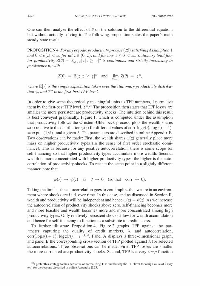
One can then analyze the effect of θ on the solution to the differential equation, but without actually solving it. The following proposition states the paper’s main steady-state result.

PROPOSITION 4: For any ergodic productivity process (25) satisfying Assumption 1 and 0 < σ (z) < ∞ for all z ∈ (0,

_ z ), and for any 1 ≤ λ < ∞, stationary total fac-

tor productivity Z(θ) = 피 ω(·, θ) [ z | z ≥ z _ ] α is continuous and strictly increasing in persistence θ, with

Z(0) = 피[ z | z ≥ z _ ] α and lim θ→∞

Z(θ) = _ z α ,

where 피[ ⋅ ] is the simple expectation taken over the stationary productivity distribu-tion ψ, and

_ z α is the first-best TFP level.

In order to give some theoretically meaningful units to TFP numbers, I normalize them by the first-best TFP level,

_ z α .34 The proposition then states that TFP losses are

smaller the more persistent are productivity shocks. The intuition behind this result is best conveyed graphically. Figure 1, which is computed under the assumption that productivity follows the Ornstein-Uhlenbeck process, plots the wealth shares ω(z) relative to the distribution ψ(z) for different values of corr[ log z(t), log z(t + 1)] = exp(− (1/θ)) and a given λ. The parameters are described in online Appendix E. Two observations can be made: First, the wealth shares ω(z) generally place more mass on higher productivity types (in the sense of first order stochastic domi-nance). This is because for any positive autocorrelation, there is some scope for self-financing so that higher productivity types accumulate more wealth. Second, wealth is more concentrated with higher productivity types, the higher is the auto-correlation of productivity shocks. To restate the same point in a slightly different manner, note that

ω(z) → ψ(z) as θ → 0 (so that corr → 0).

Taking the limit as the autocorrelation goes to zero implies that we are in an environ-ment where shocks are i.i.d. over time. In this case, and as discussed in Section II, wealth and productivity will be independent and hence ω(z) = ψ(z). As we increase the autocorrelation of productivity shocks above zero, self-financing becomes more and more feasible and wealth becomes more and more concentrated among high productivity types. Only relatively persistent shocks allow for wealth accumulation and hence for self-financing to function as a substitute to credit access.

To further illustrate Proposition 4, Figure 2 graphs TFP against the par-ameter capturing the quality of credit markets, λ, and autocorrelation, corr(log z(t + 1), log z(t)) = e −(1/θ) . Panel A displays a three-dimensional graph, and panel B the corresponding cross-section of TFP plotted against λ for selected autocorrelations. Three observations can be made. First, TFP losses are smaller the more correlated are productivity shocks. Second, TFP is a very steep function

34 I prefer this strategy to the alternative of normalizing TFP numbers by the TFP level for a high value of λ (say ten) for the reasons discussed in online Appendix E.E3.


of autocorrelation for high values of the latter. Third, the same is not true for low values of autocorrelation for which TFP is relatively flat (that is, TFP is convex as a function of autocorrelation). The steepness of TFP for high values of autocorrela-tion potentially allows for a reconciliation of some of the very different quantitative results in the literature (Buera, Kaboski, and Shin 2011; Midrigan and Xu 2014). I comment on this in detail in online Appendix H.

As a brief aside, I would like to note that for alternatives to the Ornstein-Uhlenbeck process (26) and in the extreme case of no capital markets, λ = 1, the differential equation for stationary wealth shares (22) can actually be solved in closed form. I provide two such closed-form examples in Appendix I. These examples work with unbounded productivity processes. The results regarding the persistence of shocks are qualitatively unchanged which demonstrates that they do not depend on the boundedness of the productivity process in Assumption 1.35

35 Unfortunately, it is not possible to obtain closed-form solutions for the more general case, λ > 1, or for the transitions. Also, the stochastic processes under which closed-form solutions can be obtained are empirically somewhat less plausible and harder to link to existing empirical estimates than the process (26). For instance, they are processes on the level rather than the logarithm of productivity. So as not to switch between different stochastic

Figure 1. Wealth Shares and Autocorrelation

Notes: The dashed lines are the productivity distribution ψ(z) from (27). The solid lines are the wealth shares ω(z): i.e., the solution to (22) for the stochastic process (26). As persistence θ (equivalently autocorrelation) increases, wealth becomes more concentrated with high-productivity entrepreneurs.

0 0.5 1.0 1.5 2.0 2.5 3.0 3.50

0.1

0.2

0.3

0.4

0.5

0.6

0.7ψ(z)

ω(z)

z

Panel A. Corr = 0.5

0 0.5 1.0 1.5 2.0 2.5 3.0 3.50

0.1

0.2

0.3

0.4

0.5

0.6

0.7

z

Panel B. Corr = 0.8

0 0.5 1.0 1.5 2.0 2.5 3.0 3.50

0.1

0.2

0.3

0.4

0.5

0.6

0.7

z

Panel C. Corr = 0.95

0 0.5 1.0 1.5 2.0 2.5 3.0 3.50

0.1

0.2

0.3

0.4

0.5

0.6

0.7

z

Panel D. Corr = 0.99

ω(z)

ψ(z)

ψ(z)

ω(z)

ψ(z)

ω(z)


The main purpose of this section has been to illustrate the role of the persis-tence of productivity shocks for steady-state capital misallocation and hence for TFP losses from financial frictions. I have demonstrated that even with no capital markets λ = 1 the first-best capital allocation is attainable if productivity shocks are sufficiently persistent over time. Conversely, steady-state TFP losses can be large if shocks are i.i.d. over time or close to that case.

C. The Effect of Persistence on Transition Dynamics

Having examined how steady-state productivity losses from financial frictions depend on the persistence of productivity shocks, I now turn to the transition dynamics of the model. A deeper understanding of transition dynamics allows one to answer questions such as: if a developing country undertakes a reform, how long do its residents need to wait until they see tangible results and what factors does this depend on? Related, transitions in models of financial frictions have the potential to explain observed growth episodes such as the postwar miracle economies (Buera and Shin 2013). I argue in this section that, if shocks are relatively persistent so that financial frictions are unimportant in the long-run steady state, they instead considerably slow down the transition to steady state. This is because self-financing takes time and results in the joint distribution of ability and wealth and therefore TFP evolving endogenously over time. Conversely, transitory shocks result in large long-run productivity losses but a fast transition. Furthermore, if the initial joint dis-tribution of productivity and wealth is sufficiently distorted, the case with persistent shocks and hence small long-run TFP losses, also turns out to be the case with large short-run TFP losses. My results are numerical. I would, however, like to emphasize

processes in the main text, I relegated the closed-form examples to online Appendix I. Readers with a preference for closed-form solutions should still find them appealing.

Figure 2. TFP and Autocorrelation

Notes: Panel B displays a cross-section of the three-dimensional graph in panel A. Again, note the sensitivity in the range corr = 0.75 to corr = 1. Parameters are α = 1/3, ρ = δ = 0.05, σ √

_ − log(0.85) = 0.56, and I vary

corr = exp(− (1/θ)).

Panel A

24

68

10

0

0.5

1.00.650.700.750.800.850.900.95

λCorr

TF

PPanel B

1 2 3 4 5 6 7 8 9 10

0.65

0.70

0.75

0.80

0.85

0.90

0.95

1.00

Corr = 0

Corr = 0.5Corr = 0.9

Corr = 0.99

λ

TF

P


that solving for an equilibrium boils down to solving a single partial differential equation, (21). This can be done very efficiently and I therefore view my approach as an improvement over existing techniques for computing transition dynamics in this class of models. See the discussion in footnote 6. My numerical algorithm is described in online Appendix J.

I here present three transition experiments. The first experiment follows Buera and Shin (2013) and computes transitions after a reform eliminates idiosyncratic distortions. In the prereform steady state, firms face idiosyncratic distortions (in addition to financial frictions) which are positively correlated with firm-level pro-ductivity as in Restuccia and Rogerson (2008). A reform removes these distortions and triggers a transition. Details are in online Appendix K. Buera and Shin (2013) have argued that these types of transitions capture many features of the growth expe-riences of postwar miracle economies. The second and third experiments are simply transitions from an exogenously given initial joint distribution of ability and wealth, as summarized by the corresponding wealth shares, ω 0 (z). I find it convenient to parameterize the initial wealth shares as

(29) ω 0 (z) ∝ 1 _ z exp ( − (log z − m ) 2

_ σ 2

) .

This is the formula for a log normal distribution with mean m and variance σ 2 /2. With m = 0, this is also the stationary distribution of the Ornstein-Uhlenbeck pro-cess (27), ω 0 (z) = ψ(z), meaning that wealth and ability are independent of each other at time zero. With m > 0, wealth shares place more mass on high-ability types, which is to say that wealth and ability are positively correlated. My second transi-tion experiment starts with a distorted initial allocation, in which wealth and ability are negatively correlated (m = − 0.5) and my third experiment instead starts from a relatively undistorted allocation (m = 0.25). In all experiments, I use the same parameters as in the preceding section and additionally set λ = 1.2, consistent with the external-finance-to-GDP ratio for India (see online Appendix Table E1).

The main result of this section is summarized in Figure 3 which plots the speed of these three types of transitions, as measured by the half-life of the TFP transition (i.e., the number of years until TFP has converged halfway to its new steady-state level) for different values of persistence. The figure shows that, regardless of the specific transition experiment, transitions are slower the more persistent are pro-ductivity shocks.36 The result holds unless TFP starts out exactly at its steady-state level in which case there are no dynamics and hence the half-life is zero.37 The result holds both in cases in which TFP is increasing toward its steady state and if it is decreasing.

36 The half-lives of the TFP transition are relatively short for empirically plausible values of persistence. But even transitions with a TFP half-life of only 4–7 years trigger prolonged capital transitions with half-lives of 15–25 years, consistent with the empirical evidence in Buera and Shin (2013).

37 In the figure, I do not report experiments in which TFP starts out exactly at its steady-state value. Neither do I report experiments where the economy starts out extremely close to its steady-state because numerically computing the half-life of the transition becomes exceedingly difficult. This is for example an issue in the third experiment starting from wealth shares (29) with m = 0.25 (line with crosses) for values of persistence between 0.75 and 0.82.


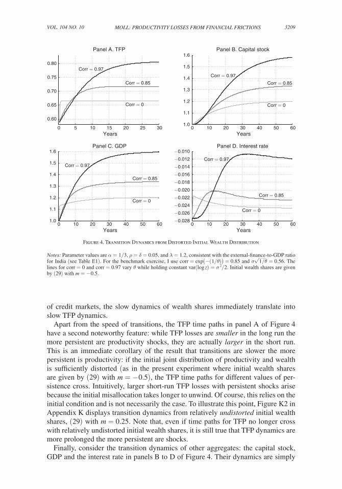
To examine this result in more detail, Figure 4 displays the second transition experiment: i.e., starting from initial wealth shares given by with (29) m = − 0.5. For now, consider only the TFP transitions in panel A. Transitions are more pro-tracted the more persistent are productivity shocks. With persistent shocks, the model generates persistent endogenous TFP dynamics while with i.i.d. shocks, TFP jumps immediately to its steady-state value.38

To understand the effect of persistence on TFP dynamics in Figures 3 and 4, it is instructive to examine the evolution of the wealth shares ω(z, t). Figure 5 plots these for two values of the autocorrelation, corr = 0 and corr = 0.97. With i.i.d. shocks (panel A), productivities are reshuffled instantaneously and wealth shares jump to their steady-state value (see footnote 39). That is, wealth shares and hence TFP do not change any more after time zero. While convergence is instantaneous, wealth and ability are independent of each other in this steady state, resulting in a relatively distorted allocation and a low level of TFP. In contrast, with persistent shocks, wealth shares continue to change for a long time. Over time, they place more and more mass on higher-productivity types—i.e., wealth gets more and more concentrated among these high-productivity types. Finally, wealth shares converge to their steady state in which wealth and productivity are positively correlated. It takes a long time to attain this more efficient allocation because initial misallocation unwinds only slowly. Since TFP depends only on the wealth shares and the quality

38 With i.i.d. shocks, wealth and productivity are immediately independent of each other (see section IF). This implies that wealth shares jump to ω(z, t) = ψ(z), the stationary productivity distribution. See panel A of Figure 5 below. In turn, TFP jumps immediately to its long-run level of E [ z | z ≥ z _ ]: i.e., a simple unweighted average of the productivities of active entrepreneurs.

0 0.2 0.4 0.6 0.8 10

1

2

3

4

5

6

7

8

Corr

Hal

f-lif

e of

TF

P tr

ansi

tion

(in y

ears

)

Experiments 1: Distortionary taxes

Experiments 2: m = −0.5

Experiments 3: m = 0.25

Figure 3. Effect of Autocorrelation on Speed of Transition


of credit markets, the slow dynamics of wealth shares immediately translate into slow TFP dynamics.

Apart from the speed of transitions, the TFP time paths in panel A of Figure 4 have a second noteworthy feature: while TFP losses are smaller in the long run the more persistent are productivity shocks, they are actually larger in the short run. This is an immediate corollary of the result that transitions are slower the more persistent is productivity: if the initial joint distribution of productivity and wealth is sufficiently distorted (as in the present experiment where initial wealth shares are given by (29) with m = − 0.5), the TFP time paths for different values of per-sistence cross. Intuitively, larger short-run TFP losses with persistent shocks arise because the initial misallocation takes longer to unwind. Of course, this relies on the initial condition and is not necessarily the case. To illustrate this point, Figure K2 in Appendix K displays transition dynamics from relatively undistorted initial wealth shares, (29) with m = 0.25. Note that, even if time paths for TFP no longer cross with relatively undistorted initial wealth shares, it is still true that TFP dynamics are more prolonged the more persistent are shocks.

Finally, consider the transition dynamics of other aggregates: the capital stock, GDP and the interest rate in panels B to D of Figure 4. Their dynamics are simply

Figure 4. Transition Dynamics from Distorted Initial Wealth Distribution

Notes: Parameter values are α = 1/3, ρ = δ = 0.05, and λ = 1.2, consistent with the external-finance-to-GDP ratio for India (see Table E1). For the benchmark exercise, I use corr = exp(−(1/θ)) = 0.85 and σ √

_ 1/θ = 0.56. The

lines for corr = 0 and corr = 0.97 vary θ while holding constant var(log z) = σ 2 /2. Initial wealth shares are given by (29) with m = − 0.5.

0 5 10 15 20 25 30

0.60

0.65

0.70

0.75

0.80

Corr = 0

Corr = 0.85

Corr = 0.97

Panel A. TFP

Years0 10 20 30 40 50 60

1.0

1.1

1.2

1.3

1.4

1.5

1.6

Corr = 0

Corr = 0.85

Corr = 0.97

Panel B. Capital stock

Years

0 10 20 30 40 50 601.0

1.1

1.2

1.3

1.4

1.5

1.6

Corr = 0

Corr = 0.85

Corr = 0.97

Panel C. GDP

Years0 10 20 30 40 50 60

−0.028

−0.026

−0.024

−0.022

−0.020

−0.018

−0.016

−0.014

−0.012

−0.010

Corr = 0

Corr = 0.85

Corr = 0.97

Panel D. Interest rate

Years


Figure 5. Transition Dynamics for Wealth Shares

Notes: Panel A displays transition dynamics for corr = 0, and panel B for corr = 0.97. With corr = 0, wealth shares jump immediately to their steady-state value which is just the stationary distribution of productivity shocks ψ(z), implying that productivity and wealth are independent in the cross-section. After time zero, wealth shares and hence TFP do not change anymore. In contrast, with corr = 0.97 wealth shares continue to change for a long time. Over time, they place more and more mass on higher productivity types: i.e., wealth gets more and more concentrated among these high-productivity types. Finally, wealth shares converge to their steady state in which wealth and pro-ductivity are positively correlated. Since TFP depends only on the wealth shares and the quality of credit markets, the slow transition of wealth shares immediately implies a slow transition of TFP.

1.0

10

043210

0

0.2

0.4

0.6

0.8

30

20

z

t

10

0

30

20

t

43210

1.0

0

0.2

0.4

0.6

0.8

ω(z,

t)

z

ω(z,

t)

Panel A. Wealth shares, corr = 0

Panel B. Wealth shares, corr = 0.97


those that would arise in a standard growth model with exogenous TFP following the time paths in panel A. For instance, consider the dynamics of the interest rate in panel D. With i.i.d. shocks, TFP jumps immediately to its steady-state value and hence interest rate dynamics are qualitatively identical to those in a growth model following a one-time permanent TFP increase: the interest rate declines monotoni-cally throughout the transition. In contrast, with persistent shocks, TFP grows over a prolonged time period and hence the interest rate rises during early stages of the tran-sition.39 King and Rebelo (1993) have argued that a neoclassical growth model with constant (or no) exogenous TFP growth has no hope of explaining sustained growth as stemming from transitional dynamics. In particular, one generates extremely counterfactual implications for the time path of the interest rate. According to their calculations, if the neoclassical growth model were to explain the postwar growth experience of Japan, the interest rate in 1950 should have been around 500 per-cent. In contrast, Chen, Imrohoroglu, and Imrohoroglu (2006, 2007) argue that the neoclassical growth model is, in fact, consistent with the Japanese postwar growth experience once one takes as given the time-varying TFP path measured in the data. The time path for TFP in panel A of Figure 4 that my model with persistent shocks generates endogenously is, in fact, broadly similar to the exogenous time path that Chen, Imrohoroglu, and Imrohoroglu feed into their neoclassical growth model.40 But note that only the version of the model with persistent shocks can generate these dynamics whereas the version with i.i.d. shocks cannot.

D. Welfare

If the persistence of productivity shocks affects TFP and GDP losses differen-tially in steady state and during transitions, one may ask how these effects should be balanced against each other. The welfare measure in Lemma 3 provides a natu-ral metric. Figure 6 plots various welfare measures relative to their first-best val-ues against autocorrelation. These welfare numbers are in permanent consumption equivalents.41 The initial wealth shares are those from Figure 4. Panel A plots wel-fare of workers,

_ V 0 W , against autocorrelation for two values of the discount rate ρ.

Because workers’ welfare simply equals the present discounted value of wages and wage payments are a constant fraction of GDP, it simply trades off the short run and the long run of the GDP time paths in panel C of Figure 4. For reasonable values of the discount rate ρ, the long run dominates and workers’ welfare is an increasing

39 This is a statement about the slope of the interest rate time path; still some readers may wonder about its level, namely why real interest rates are negative. Interest rates are bounded below by − δ and negative real interest rates due to depressed credit demand are a common feature of models with collateral constraints (Buera and Shin 2013; Buera, Kaboski, and Shin 2011; Guerrieri and Lorenzoni 2011). The particular form of the borrowing constraint (4) does matter. For instance, negative interest rates are less likely to occur if the maximum leverage ratio is decreasing in the interest rate as in the extension in Appendix D (equation (D4)). Even with the constraint (4), many alternative parameterizations feature positive interest rates.

40 See Table A1 in Chen, Imrohoroglu, and Imrohoroglu (2006) and Figure 9 in Chen, Imrohoroglu, and Imrohoroglu (2007) for the TFP growth rates they feed into their model. As in panel A of Figure 4 for the case corr = 0.97, the Japanese TFP growth rate starts out positive in 1956 and then converges to zero toward 2000. My model has no aggregate uncertainty so cannot generate the deviations from trend that are features of the Japanese TFP time-path. But the underlying trend is similar to that generated by my model in terms of both magnitude and speed of transition.

41 That is, consider _ V t defined in (24). By permanent consumption equivalents I mean

_ C 0 satisfying

_ V 0 = log(

_ C 0 )/ρ so that Figure 6 reports

_ C 0 /

_ C 0 FB = exp[ρ (

_ V 0 −

_ V 0 FB ) ].


function of autocorrelation. But this relationship is flatter when workers are more myopic (higher ρ).42 Panel B shows that entrepreneurial welfare,

_ V 0 E is a (barely)

hump-shaped function of autocorrelation in the case where ρ = 0.05. This result has been discussed in detail by Buera and Shin (2011) and is due to two offsetting effects: on one hand, more persistent shocks lead to higher total factor productivity and hence higher returns to capital; on the other hand, more persistent shocks are harder to self-insure.43 Panels C and D plot overall welfare

_ V 0 for two different val-

ues of the Pareto weight Θ that the planner places on workers: i.e., simple weighted averages of

_ V 0 W and

_ V 0 E in panels A and B. Depending on the Pareto weight, the

42 For extremely high values of the discount rate ρ, and given a distorted initial allocation as in the present exer-cise, workers’ welfare can be a decreasing function of autocorrelation because the high short-run GDP losses with persistent shocks outweigh the low steady-state losses.

43 See Figure 1 in Buera and Shin (2011) which closely resembles my Figure 6 and the surrounding discussion.

Figure 6. Welfare Losses

Notes: Parameter values are α = 1/3, δ = 0.05, and λ = 1.2, consistent with the external-finance-to-GDP ratio for India (see Table E1), and I vary corr = exp(−(1/θ)) while holding constant var(log z) = σ 2 /2 = (0.56 ) 2 /(− 2log(0.85)) = 0.96. Initial wealth shares are the same as in Figure 4 and given by (29) with m = − 0.5. Welfare relative to first-best is in units of permanent consumption:

_ C 0 /

_ C 0 FB = exp[ρ (

_ V 0 −

_ V 0 FB ) ]

where _ V 0 is defined in (24).

0 0.2 0.4 0.6 0.8 10.58

0.60

0.62

0.64

0.66

0.68

0.70

0.72

0.74

ρ = 0.05ρ = 0.1

Panel A. Welfare of workersW

elfa

re r

elat

ive

to fi

rst−

best

corr0 0.2 0.4 0.6 0.8

0.40

0.45

0.50

0.55

0.60

0.65

0.70

0.75

ρ = 0.05

ρ = 0.1

Panel B. Welfare of entrepreneurs

Wel

fare

rel

ativ

e to

firs

t−be

st

corr

0 0.2 0.4 0.6 0.80.55

0.6

0.65

ρ = 0.05

ρ = 0.1

Panel C. Total welfare with worker weight, Θ = 0.5

Wel

fare

rel

ativ

e to

firs

t−be

st

corr0 0.2 0.4 0.6 0.8 1

0.59

0.60

0.61

0.62

0.63

0.64

0.65

0.66

ρ = 0.05

ρ = 0.1

Panel D. Total welfare with worker weight, Θ = 0.7

Wel

fare

rel

ativ

e to

firs

t−be

st

corr


shape of overall welfare as a function of persistence can be extremely different. Summarizing, the effect of persistence on overall welfare is ambiguous depending on the discount rate and the Pareto weights of workers and entrepreneurs.

E. Summary of Results

To summarize, consider the behavior of my model with a persistence parameter in the empirically relevant range: i.e., with an autocorrelation of, say, 0.75 to 0.97 (Gourio 2008; Asker, Collard-Wexler, and De Loecker forthcoming). With such a level of persistence, financial frictions can matter in both the short and the long run. In the long run, self-financing partly undoes capital misallocation and hence reduces TFP losses; but the steepness of steady-state TFP for high values of autocorrela-tion (see Figure 2) means that even relatively persistent shocks can lead to sizable steady-state TFP losses. At the same time, financial frictions provide a theory of endogenous TFP dynamics that result in prolonged transitions to steady state for capital and GDP. In contrast, the empirically irrelevant extremes of fixed productivi-ties and i.i.d. shocks are potentially misleading but for completely different reasons: with fixed productivities, self-financing completely undoes all capital misallocation in the long-run and TFP is first-best; in contrast, with i.i.d. shocks the model gener-ates no endogenous TFP dynamics as TFP jumps immediately to its steady-state value. Finally, in the empirically relevant range, financial frictions result in welfare losses for both workers and entrepreneurs, and higher persistence makes workers better off but entrepreneurs worse off so that the overall effect is ambiguous.

III. Sensitivity to Functional Form Assumptions

To deliver my model’s tractability, I have assumed that entrepreneurs have loga-rithmic utility functions and operate constant returns to scale production functions. The purpose of this section is to briefly discuss to what extent these twin restrictions on preferences and technology can be relaxed. All detailed derivations, proofs, and computations are in online Appendix D.

Logarithmic Utility.—It is natural to ask whether results generalize to the case where entrepreneurs have constant relative risk aversion (CRRA) utility functions.44 First, the representation of aggregate GDP in terms of an aggregate production function (11) and the formula for TFP (13) follow from firms’ profit maximization behavior only and so are unchanged. What does change is entrepreneurs’ savings behavior (Lemma 2), but I now show that Propositions 1 and 2 still go through with slight modification. To see this, note that with CRRA utility with parameter γ, say, entrepreneurs still consume a constant fraction of their wealth, c = c (z, t; γ, λ)a, but

44 One may also ask whether results generalize beyond the CRRA case (say to the hyperbolic absolute risk aver-sion (HARA) class of utility functions). This extension would require a purely numerical solution and most tracta-bility would be lost. The reason is that with rate of return risk as in the present paper, only the CRRA utility function delivers consumption policy functions that are linear in wealth (Carroll and Kimball 1996). And this is exactly what allows individual savings rules to be aggregated. However, note that CRRA utility is the standard assumption made by the entire quantitative literature discussed in the introduction.


this marginal propensity to consume is no longer constant across productivity types. In the special case of log utility, c (z, t; 1, λ) = ρ. Further, define by

(30) ρ (t; γ, λ) = ∫ 0 ∞ c (z, t; γ, λ) ω(z, t) dz

the aggregate marginal propensity to consume out of wealth. Proposition 1 then goes through with one modification only, namely that we need to replace ρ by ρ (t; γ, λ) in equation (12). Similarly, in Proposition 2 only the definition of the savings rate needs to be changed to reflect the changed marginal propensity to consume.45

With these modified propositions in hand, we can now examine the robust-ness of the paper’s main results to departures from log utility. First, my economy still aggregates to a Solow model, however now with a time-varying depreciation rate, δ (t; γ, λ) = ρ (t; γ, λ) + δ, that potentially depends on financial development λ. As a corollary, consider the result from Section I that financial frictions affect aggregate savings only through TFP. In general, this is no longer true with CRRA utility. To see this clearly, consider the expression for the steady-state capital to out-put ratio (19) which becomes

K _ Y

= α _ ρ (γ, λ) + δ

.

Because in general the aggregate marginal propensity to consume ρ (γ, λ) depends on λ, so does K/Y. While the result is therefore exact only for logarithmic utility, it turns out that the capital to output ratio does not change much with λ as long as γ is close to 1. Put differently, things are continuous in γ. To make this point, I have computed numerical examples in which I vary λ over the empirically plausible range from 1 to 4.15 (the latter corresponding to my estimate for the United States, see online Table E1) and then examine changes in K/Y for different values of γ. For γ = 2, K/Y changes by 8 percent; and for γ = 1/2, it changes by 3 percent only. Furthermore, note that the direct effect of λ on aggregate savings is really due to individual marginal utilities not being equalized under incomplete markets, rather than marginal products not being equalized due to collateral constraints.46

Next, consider the result that steady-state TFP losses are strictly decreasing in the persistence of productivity shocks, θ. In contrast to Proposition 4, it is no longer possible to prove this result analytically.47 However, the result continues to hold in all my numerical experiments, again using standard parameter values. Finally, also

45 That is, s (z) ≡ λ max{zπ − r − δ, 0} + r − c (z; γ, λ) which generalizes s(z) in Lemma 2.46 Consistent with this, and as in Angeletos (2007) who analyzes an economy without collateral constraints,

whether K/Y is greater or smaller than in the perfect credit/complete markets benchmark, α/(ρ + δ), depends on γ. If γ < 1, the capital-output ratio is smaller; if γ > 1, it is larger. Similarly, K/Y is an increasing function of λ with γ < 1 but a decreasing one with γ > 1. See also Buera and Moll (2012) who show how, in my framework with log utility, individual Euler equations can be aggregated to an Euler equation for the representative entrepreneur, and that with CRRA utility one picks up additional aggregation effects due to incomplete insurance.

47 This is because with the process (25), the marginal propensity to consume c (z; γ, λ, θ) and hence the savings rate s (z) ≡ λ max{zπ − r − δ, 0} + r − c (z; γ, λ, θ) depend on θ, so that there is an additional effect which cannot be signed in general.


the result that transitions are slow if shocks are persistent continues to hold with CRRA utility with the same parameter values.

Constant Returns Technology.—Things change more substantially if I drop the assumption that entrepreneurs operate constant returns to scale technologies. With decreasing returns, individual firm size is no longer constrained by wealth only and hence capital demand is no longer linear in wealth. This implies that it is no longer possible to represent aggregate GDP in terms of an aggregate production function as in (11) or to obtain a simple formula for TFP like (13). This being said, note that everything is continuous in returns to scale. For example, with constant returns all active firms are financially constrained; and with returns to scale slightly below 1, almost all firms are constrained. Therefore the constant returns economy analyzed in the present paper is simply the analytically tractable limiting case of a decreasing returns economy. In Appendix G, I make this point more formally by assuming that production functions are y = ((zk ) α ℓ 1−α ) ν , ν < 1 rather than (2) and by showing that many of my formulas for the production side of the economy can be obtained by taking the limit as ν → 1.48 My paper analyzes the analytically tractable limiting case of constant returns to scale, whereas most of the existing literature analyzes the empirically more relevant but intractable case of decreasing returns. I view the two approaches as complimentary.49 Standard values for ν are relatively close to 1,50 so there is some reason to believe that my results would continue to hold. In line with this, the recent quantitative literature analyzing decreasing returns environ-ments provides some illustrative calculations regarding the effect of persistence on steady-state TFP losses that closely mirror my analytical results.51

IV. Concluding Remarks

In my framework, self-financing undoes capital misallocation from financial fric-tions in the long run if idiosyncratic productivity shocks are relatively persistent. The reason is that entrepreneurs accumulate wealth out of past successes so only if high productivity episodes are sufficiently prolonged can they accumulate sufficient internal funds to self-finance their desired investments. As a result, the extent of steady-state capital misallocation and therefore TFP losses from financial frictions are small with persistent shocks. However, the case in which steady-state productiv-ity losses are small is precisely the case in which transitions to this steady state take a very long time. This is because TFP endogenously evolves as capital misallocation slowly unwinds over time. Conversely, if shocks are transitory, steady-state TFP losses are large but the transition to this steady state is fast.

48 Just to give an example, first-best TFP is a geometric mean of productivities Z FB (ν) = ( ∫ 0 _ z z

α _ 1−ν

ψ(z) dz ) 1−ν which satisfies lim ν→1 Z FB (ν) = max{ z α } =

_ z α .

49 The decreasing returns case is arguably more useful for studying firm-level facts—e.g., firm dynamics and size distributions, and for a serious quantitative assessment of aggregate TFP losses from financial frictions.

50 For example, ν is 0.85 in Atkeson and Kehoe (2007) and Midrigan and Xu (2014), and 0.79 in Buera and Shin (2013).

51 See Figure 2 in Buera and Shin (2011) showing that steady-state TFP losses are strictly decreasing in persis-tence, and the robustness checks in Midrigan and Xu (2010, the working paper version). The robustness checks in Buera and Shin (2013) suggest that also my transition results carry over to the decreasing returns case.


I have made this point in a heterogeneous-agent model with borrowing con-straints and forward-looking savings behavior. While featuring rich heterogeneity, the model remains highly tractable and TFP is simply a truncated weighted average of individual productivities, where the weights are the shares of wealth held by dif-ferent productivity types. Solving for an equilibrium boils down to solving a single differential equation for these wealth shares (Proposition 2) which is a substantial improvement over commonly used solution techniques. In contrast to similar exist-ing theories, the model presented here also allows for persistent productivity shocks. The self-financing mechanism that takes center stage in my paper implies that any empirically serious theory of heterogeneous firms and financial frictions must fea-ture such persistence. The tools presented in this paper, particularly Propositions 2 and 4, could therefore also prove useful in other applications.

Appendix: Proofs

A1. Proof of Lemma 1

From the profit maximization problem (5), optimal labor demand is ℓ = (π/α ) 1/(1−α) zk, where π is as in the lemma. Plugging back in, the profit function becomes

Π(a, z) = max k {zπk − (r + δ)k s.t. k ≤ λa}.

Since this problem is linear, it follows immediately that k is either zero or λa. The cutoff z _ is defined as the value for which entrepreneurs are indifferent between run-ning a firm and being inactive, Π(a, z _ ) = 0.


From Lemma 1, we know that a = A(z, t)a − c where A(z, t) = λ max{zπ(t) − r(t) − δ, 0} + r(t). The Bellman equation is then (see Stokey 2009, ch. 2),

ρV(a, z, t) = max c { log c + 1 _

dt 피 [ dV(a, z, t)] s.t. da = [ A(z, t) − c ]dt } .

The proof proceeds with a guess and verify strategy. Guess that the value func-tion takes the form V(a, z, t) = Bv(z, t) + B log a. Using this guess we have that E [dV(a, z, t)] = (B/a)da + BE [dv(z, t)]. Rewrite the value function

ρBv(z, t) + ρB log a = max c log c + B _ a [ A(z, t)a − c ] + B 1 _

dt 피 [dv(z, t)].

Take first-order condition to obtain c = a/B. Substituting back in,

ρBv(z, t) + ρB log a = log a − log B + A(z, t)B − 1 + B 1 _ dt

피 [dv(z, t)].


Collecting the terms involving log a, we see that B = 1/ρ so that c = ρa and a = [A(z, t) − ρ]a as claimed. Finally, the value function is V(a, z, t) = [v(z, t) + log a]/ρ where v(z, t) satisfies

(A1) ρv(z, t) = ρ log ρ − ρ + A(z, t) + 1 _ dt

피 [dv(z, t)].

A3. Proof of Proposition 1

Throughout this proof, I omit indexing by t for notational simplicity. Using the expression for factor demands in Lemma 1, labor demand can be written as

(A2) ℓ(a, z) = ( π _ α ) 1/(1−α) λaz, z ≥ z _ ,

and zero otherwise. It follows that individual output is y(a, z) = (π/α)λaz, if z ≥ z _ , and zero otherwise. Aggregate output is then

(A3) Y = ∫ 0 ∞ ∫

0 ∞ y(a, z) g(a, z) da dz = π _ α λ XK, where X = ∫

z _ ∞ zω(z) dz

is an auxiliary variable. Next, consider the labor market clearing condition (A2). Integrating over all a and z,

(A4) L = ( π _ α ) 1/(1−α) λ XK ⇔ π = α(λ X ) α−1 K α−1 L 1−α .

Substituting into (11), we see that Y = (λ XK ) α L 1−α . Eliminating λ using (14) this is (11) and (13) in the proposition.

Consider next the law of motion for aggregate capital (10). Using that the shares ω(z) integrate to 1, we have that

K _ K

= λ π ∫ z _ ∞ zω(z) dz − λ(r + δ ) ∫

z _ ∞ ω(z) dz + r − ρ.

Using capital market clearing (14),

(A5) K _ K

= λ πX − (ρ + δ), X ≡ ∫ z _ ∞ zω(z) dz.

Substituting (A4) into (A5) and rearranging, we get

K = αZ K α L 1−α − (ρ + δ)K, Z = (λX ) α .

After substituting for λ from (14), this is equation (12) in Proposition 1. Substituting the definition of π from Lemma 1 into (A4) and rearranging yields the expression for w. Substituting (A4) into the cutoff condition z _ π = R and rearranging yields the expression for R.


A4. Proof of Proposition 2

The law of motion for the joint distribution of wealth is given by the Kolmogorov Forward Equation (see for example Stokey 2009, p. 50).

(A6) ∂g(a, z, t) _

∂t = − ∂ _

∂a [ g(a, z, t) s(z, t)a ] − ∂ _

∂z [ g(a, z, t) μ(z) ]

+ 1 _ 2 ∂ 2 _ ∂ z 2

[ σ 2 (z) g(a, z, t) ] .

Using the definition of ω(z, t) we have that

(A7) ∂ω(z, t) _

∂t = 1 _

K(t) ∫

0 ∞ a

∂g(a, z, t) _

∂t da −

K (t) _

K(t) ω(z, t).

Using an integration by parts

(A8) − ∫ 0 ∞ a ∂ _

∂a [ g(a, z, t) s(z, t)a ] da = s(z, t) ∫

0 ∞ ag(a, z, t) da.

Plugging (A6) into (A7) and using (A8), we obtain the PDE (21). Setting the time derivative equal to zero, one obtains the ODE (22). This proves all assertions in the theorem except for continuity and differentiability, which require more work. Due to space constraints these proofs are stated in online Appendix B3.


Welfare at time t is given by

(A9) _ V t = ( 1 − Θ ) ∫

V(a, z, t) d G t (a, z) + Θ ∫ t ∞ e −ρ(s−t) log[ w(s) L] ds.

From the proof of Lemma 2, the value function of an entrepreneur is V(a, z, t) = [v(z, t) + log a]/ρ where v(z, t) satisfies (A1). Substituting into (A9) gives (24). With the stochastic process (20), (A1) is

(A10) ρv(z, t) = ρ log ρ − ρ + λ max{zπ(t) − r(t) − δ, 0} + r(t)

+ ∂v(z, t) _

∂z μ(z) + 1 _

2

∂ 2 v(z, t) _

∂ z 2 σ 2 (z) +

∂ v(z, t) _

∂ t .

A6. Proofs of Propositions 3 and 4

The proofs are long and mathematically involved and stated in online Appendix B.


REFERENCES

Aghion, Philippe, and Patrick Bolton. 1997. “A Theory of Trickle-Down Growth and Development.” Review of Economic Studies 64 (2): 151–72.

Amaral, Pedro S., and Erwan Quintin. 2010. “Limited Enforcement, Financial Intermediation, and Economic Development: A Quantitative Assessment.” International Economic Review 51 (3): 785–811.

Angeletos, George-Marios. 2007. “Uninsured Idiosyncratic Investment Risk and Aggregate Saving.” Review of Economic Dynamics 10 (1): 1–30.

Asker, John, Allan Collard-Wexler, and Jan De Loecker. Forthcoming. “Dynamic Inputs and Resource (Mis)Allocation.” Journal of Political Economy.

Atkeson, Andrew, and Patrick J. Kehoe. 2007. “Modeling the Transition to a New Economy: Lessons from Two Technological Revolutions.” American Economic Review 97 (1): 64–88.

Azariadis, Costas, and Leo Kaas. 2012. “Capital Misallocation and Aggregate Factor Productivity.” Federal Reserve Bank of St. Louis Working Paper 2012-046.

Banerjee, Abhijit V., and Esther Duflo. 2005. “Growth Theory through the Lens of Development Eco-nomics.” In Handbook of Economic Growth. Vol. 1, Part A, edited by Philippe Aghion and Steven Durlauf, 473–554. Amsterdam: Elsevier B.V.

Banerjee, Abhijit V., and Benjamin Moll. 2010. “Why Does Misallocation Persist?” American Eco-nomic Journal: Macroeconomics 2 (1): 189–206.

Banerjee, Abhijit V., and Andrew F. Newman. 1993. “Occupational Choice and the Process of Devel-opment.” Journal of Political Economy 101 (2): 274–98.

Banerjee, Abhijit V., and Andrew F. Newman. 2003. “Inequality, Growth and Trade Policy.” Unpub-lished.

Bartelsman, Eric, John Haltiwanger, and Stefano Scarpetta. 2013. “Cross-Country Differences in Pro-ductivity: The Role of Allocation and Selection.” American Economic Review 103 (1): 305–34.

Bénabou, Roland. 2002. “Tax and Education Policy in a Heterogenous-Agent Economy: What Levels of Redistribution Maximize Growth and Effiency?” Econometrica 70 (2): 481–517.

Benhabib, Jess, Alberto Bisin, and Shenghao Zhu. 2011. “The Distribution of Wealth and Fiscal Policy in Economies with Finitely Lived Agents.” Econometrica 79 (1): 123–57.

Blaum, Joaquin. 2012. “Wealth Inequality and the Losses from Financial Frictions.” Unpublished.Buera, Francisco J. 2009. “A Dynamic Model of Entrepreneurship with Borrowing Constraints: The-

ory and Evidence.” Annals of Finance 5 (3–4): 443–64.Buera, Francisco J., Joseph P. Kaboski, and Yongseok Shin. 2011. “Finance and Development: A Tale

of Two Sectors.” American Economic Review 101 (5): 1964–2002.Buera, Francisco J., and Benjamin Moll. 2012. “Aggregate Implications of a Credit Crunch.” National

Bureau of Economic Research Working Paper 17775.Buera, Francisco J., and Yongseok Shin. 2011. “Self-insurance vs. Self-financing: A Welfare Analysis

of the Persistence of Shocks.” Journal of Economic Theory 146 (3): 845–62.Buera, Francisco J., and Yongseok Shin. 2013. “Financial Frictions and the Persistence of History:

A Quantitative Exploration.” Journal of Political Economy 121 (2): 221–72.Carroll, Christopher D., and Miles S. Kimball. 1996. “On the Concavity of the Consumption Func-

tion.” Econometrica 64 (4): 981–92.Caselli, Francesco, and James Feyrer. 2007. “The Marginal Product of Capital.” Quarterly Journal of

Economics 122 (2): 535–68.Caselli, Francesco, and Nicola Gennaioli. 2013. “Dynastic Management.” Economic Inquiry 51 (1):

971–96.Chen, Kaiji, Ayse Imrohoroglu, and Selahattin Imrohoroglu. 2006. “The Japanese Saving Rate.”

American Economic Review 96 (5): 1850–8.Chen, Kaiji, Ayse Imrohoroglu, and Selahattin Imrohoroglu. 2007. “The Japanese Saving Rate

between 1960 and 2000: Productivity, Policy Changes, and Demographics.” Economic Theory 32 (1): 87–104.

Dasgupta, Partha, and Debraj Ray. 1986. “Inequality as a Determinant of Malnutrition and Unem-ployment: Theory.” Economic Journal 96 (384): 1011–34.

Dixit, Avinash K., and Robert S. Pindyck. 1994. Investment Under Uncertainty. Princeton: Princeton University Press.

Erosa, Andrés, and Ana Hidalgo-Cabrillana. 2008. “On Finance as a Theory of TFP, Cross-Industry Productivity Differences, and Economic Rents.” International Economic Review 49 (2): 437–73.

Fouque, Jean-Pierre, George Papanicolaou, Ronnie Sircar, and Knut Solna. 2011. Multiscale Stochas-tic Volatility for Equity, Interest Rate, and Credit Derivatives. Cambridge: Cambridge University Press.

http://pubs.aeaweb.org/action/showLinks?crossref=10.1162%2Fqjec.122.2.535

http://pubs.aeaweb.org/action/showLinks?crossref=10.3982%2FECTA8416

http://pubs.aeaweb.org/action/showLinks?crossref=10.1111%2Fj.1465-7295.2012.00467.x

http://pubs.aeaweb.org/action/showLinks?system=10.1257%2Faer.97.1.64


http://pubs.aeaweb.org/action/showLinks?crossref=10.1007%2Fs10436-009-0121-2



http://pubs.aeaweb.org/action/showLinks?system=10.1257%2Fmac.2.1.189

http://pubs.aeaweb.org/action/showLinks?crossref=10.2307%2F2233171


http://pubs.aeaweb.org/action/showLinks?crossref=10.1016%2Fj.jet.2011.01.003






http://pubs.aeaweb.org/action/showLinks?crossref=10.1016%2Fj.red.2006.11.001


http://pubs.aeaweb.org/action/showLinks?crossref=10.1111%2F1468-0262.00293


Gabaix, Xavier. 2009. “Power Laws in Economics and Finance.” Annual Review of Economics 1 (1): 255–93.

Galor, Oded, and Joseph Zeira. 1993. “Income Distribution and Macroeconomics.” Review of Eco-nomic Studies 60 (1): 35–52.

Gentry, William M., and R. Glenn Hubbard. 2004. “Entrepreneurship and Household Saving.” Advances in Economic Analysis and Policy 4 (1): 1–55.

Giné, Xavier, and Robert M. Townsend. 2004. “Evaluation of Financial Liberalization: A General Equilibrium Model with Constrained Occupation Choice.” Journal of Development Economics 74 (2): 269–307.

Gourio, François. 2008. “Estimating Firm-Level Risk.” Unpublished.Guerrieri, Veronica, and Guido Lorenzoni. 2011. “Credit Crises, Precautionary Savings, and the

Liquidity Trap.” National Bureau of Economic Research Working Paper 17583.Hall, Robert E., and Charles I. Jones. 1999. “Why Do Some Countries Produce So Much More Output

Per Worker Than Others?” Quarterly Journal of Economics 114 (1): 83–116.Hsieh, Chang-Tai, and Peter J. Klenow. 2007. “Relative Prices and Relative Prosperity.” American

Economic Review 97 (3): 562–85.Hsieh, Chang-Tai, and Peter J. Klenow. 2009. “Misallocation and Manufacturing TFP in China and

India.” Quarterly Journal of Economics 124 (4): 1403–48.Jeong, Hyeok, and Robert M. Townsend. 2007. “Sources of TFP Growth: Occupational Choice and

Financial Deepening.” Economic Theory 32 (1): 179–221.Jeong, Hyeok, and Robert M. Townsend. 2008. “Growth and Inequality: Model Evaluation Based on

an Estimation-Calibration Strategy.” Macroeconomic Dynamics 12: 231–84.Kehoe, Timothy J., and David K. Levine. 2001. “Liquidity Constrained Markets versus Debt Con-

strained Markets.” Econometrica 69 (3): 575–98.King, Robert G., and Sergio T. Rebelo. 1993. “Transitional Dynamics and Economic Growth in the

Neoclassical Model.” American Economic Review 83 (4): 908–31.Kiyotaki, Nobuhiro. 1998. “Credit and Business Cycles.” Japanese Economic Review 49 (1): 18–35.Kiyotaki, Nobuhiro, and John Moore. 2012. “Liquidity, Business Cycles, and Monetary Policy.”

National Bureau of Economic Research Working Paper 17934.Klenow, Peter J., and Andrés Rodríguez-Clare. 1997. “The Neoclassical Revival in Growth Econom-

ics: Has It Gone Too Far?” In NBER Macroeconomics Annual 1997. Vol. 12, edited by Ben S. Ber-nane and Julio J. Rotemberg, 73–114. Cambridge: MIT Press.

Kocherlakota, Narayana R. 2009. “Bursting Bubbles: Consequences and Cures.” Unpublished.Krebs, Tom. 2003. “Human Capital Risk and Economic Growth.” Quarterly Journal of Economics

118 (2): 709–44.Lagos, Ricardo. 2006. “A Model of TFP.” Review of Economic Studies 73 (4): 983–1007.Levine, Ross. 2005. “Finance and Growth: Theory and Evidence.” In Handbook of Economic Growth.

Vol. 1, Part A, edited by Philippe Aghion and Steven Durlauf, 865–934. Amsterdam: Elsevier B.V. Ljungqvist, Lars. 1993. “Economic Underdevelopment: The Case of a Missing Market for Human

Capital.” Journal of Development Economics 40 (2): 219–39.Lucas, Robert E., Jr. 1990. “Why Doesn’t Capital Flow from Rich to Poor Countries?” American Eco-

nomic Review 80 (2): 92–6.Matsuyama, Kiminori. 2007. “Aggregate Implications of Credit Market Imperfections.” In NBER

Macroeconomics Annual 2007, Vol. 22, edited by Daron Acemoglu, Kenneth Rogoff, and Michael Woodford, 1–60.

Midrigan, Virgiliu, and Daniel Yi Xu. 2010. “Finance and Misallocation: Evidence from Plant-level Data.” National Bureau of Economic Research Working Paper 15647.

Midrigan, Virgiliu, and Daniel Yi Xu. 2014. “Finance and Misallocation: Evidence from Plant-Level Data.” American Economic Review 104 (2): 422–58.

Moll, Benjamin. 2012. “Inequality and Financial Development: A Power-Law Kuznets Curve.” Unpub-lished.

Moll, Benjamin. 2014. “Productivity Losses from Financial Frictions: Can Self-Financing Undo Capital Misallocation?: Dataset.” American Economic Review. http://dx.doi.org/10.1257.aer.104.10.3186.

Mookherjee, Dilip, and Debraj Ray. 2003. “Persistent Inequality.” Review of Economic Studies 70 (2): 369–93.

Piketty, Thomas. 1997. “The Dynamics of the Wealth Distribution and the Interest Rate with Credit Rationing.” Review of Economic Studies 64 (2): 173–89.

Quadrini, Vincenzo. 2009. “Entrepreneurship in Macroeconomics.” Annals of Finance 5 (3–4): 295–311.

Quintin, Erwan. 2008. “Limited Enforcement and the Organization of Production.” Journal of Macro-economics 30 (3): 1222–45.

http://dx.doi.org/10.1257.aer.x.x

http://pubs.aeaweb.org/action/showLinks?crossref=10.1162%2Fqjec.2009.124.4.1403

http://pubs.aeaweb.org/action/showLinks?crossref=10.1146%2Fannurev.economics.050708.142940






http://pubs.aeaweb.org/action/showLinks?crossref=10.1111%2Fj.1467-937X.2006.00405.x


http://pubs.aeaweb.org/action/showLinks?crossref=10.1016%2Fj.jdeveco.2003.03.005

http://pubs.aeaweb.org/action/showLinks?crossref=10.1111%2F1467-937X.00248


http://pubs.aeaweb.org/action/showLinks?crossref=10.1016%2F0304-3878%2893%2990084-Z




http://pubs.aeaweb.org/action/showLinks?crossref=10.1016%2Fj.jmacro.2007.05.005



Rajan, Raghuram G., and Luigi Zingales. 1998. “Financial Dependence and Growth.” American Eco-nomic Review 88 (3): 559–86.

Restuccia, Diego, and Richard Rogerson. 2008. “Policy Distortions and Aggregate Productivity with Heterogeneous Plants.” Review of Economic Dynamics 11 (4): 707–20.

Samphantharak, Krislert, and Robert M. Townsend. 2009. Households as Corporate Firms: Con-structing Financial Statements from Integrated Household Surveys. Cambridge: Cambridge Uni-versity Press.

Solow, R. M. 1956. “A Contribution to the Theory of Economic Growth.” Quarterly Journal of Eco-nomics 70 (1): 65–94.

Stokey, Nancy L. 2009. The Economics of Inaction: Stochastic Control Models with Fixed Costs. Princeton: Princeton University Press.

Townsend, Robert. 2010. “Financial Structure and Economic Welfare: Applied General Equilibrium Development Economics.” Annual Review of Economics 2 (1): 507–46.

Wong, Eugene. 1964. “The Construction of a Class of Stationary Markoff Processes.” In Stochastic Processes in Mathematical Physics and Engineering, edited by Richard Bellman, 264–76. Provi-dence: American Mathematical Society.

http://pubs.aeaweb.org/action/showLinks?crossref=10.1016%2Fj.red.2008.05.002


http://pubs.aeaweb.org/action/showLinks?crossref=10.1146%2Fannurev.economics.102308.124427

Productivity Losses from Financial Frictions: Can Self ...moll/TFPFF.pdf · Productivity Losses...

Documents

Transcript of Productivity Losses from Financial Frictions: Can Self ...moll/TFPFF.pdf · Productivity Losses...