Mining Topological Structure in Graphs through Forest ...
68
Journal of Machine Learning Research 21 (2020) 1-68 Submitted 12/19; Revised 9/20; Published 10/20 Mining Topological Structure in Graphs through Forest Representations Robin Vandaele 1,2 [email protected] Yvan Saeys 2 [email protected] Tijl De Bie 1 [email protected] 1 IDLab, Department of Electronics and Information Systems Ghent University Technologiepark-Zwijnaarde 19, 9052 Gent, Belgium 2 Data mining and Modelling for Biomedicine (DaMBi), VIB Inflammation Research Center Technologiepark-Zwijnaarde 927, 9052 Gent, Belgium Editor: Karsten Borgwardt Abstract We consider the problem of inferring simplified topological substructures—which we term backbones —in metric and non-metric graphs. Intuitively, these are subgraphs with ‘few’ nodes, multifurcations, and cycles, that model the topology of the original graph well. We present a multistep procedure for inferring these backbones. First, we encode local (geomet- ric) information of each vertex in the original graph by means of the boundary coefficient (BC) to identify ‘core’ nodes in the graph. Next, we construct a forest representation of the graph, termed an f -pine, that connects every node of the graph to a local ‘core’ node. The final backbone is then inferred from the f -pine through CLOF (Constrained Leaves Optimal subForest ), a novel graph optimization problem we introduce in this pa- per. On a theoretical level, we show that CLOF is NP-hard for general graphs. However, we prove that CLOF can be efficiently solved for forest graphs, a surprising fact given that CLOF induces a nontrivial monotone submodular set function maximization problem on tree graphs. This result is the basis of our method for mining backbones in graphs through forest representation. We qualitatively and quantitatively confirm the applicabil- ity, effectiveness, and scalability of our method for discovering backbones in a variety of graph-structured data, such as social networks, earthquake locations scattered across the Earth, and high-dimensional cell trajectory data. Keywords: topological data analysis, graph mining, metric spaces, visualization, topo- logical skeletonization, cluster coefficient, cell trajectory inference 1. Introduction Motivation. Many real-world graphs, whether given (social networks, road networks, image webs, . . . ) or derived from point cloud data (gene expression data of differentiating cells, GPS traces, earthquake locations, galaxy coordinates in space, . . . ), exhibit topologies of which the underlying structure can be naturally represented using a much ‘simpler’ subgraph, as shown in Figure 1d. I.e., although the topology of the original graph might c 2020 Robin Vandaele, Yvan Saeys, and Tijl De Bie. License: CC-BY 4.0, see https://creativecommons.org/licenses/by/4.0/. Attribution requirements are provided at http://jmlr.org/papers/v21/19-1032.html.
Transcript of Mining Topological Structure in Graphs through Forest ...

Journal of Machine Learning Research 21 (2020) 1-68 Submitted 12/19; Revised 9/20; Published 10/20
Mining Topological Structure in Graphsthrough Forest Representations
Robin Vandaele1,2 [email protected]
Yvan Saeys2 [email protected]
Tijl De Bie1 [email protected], Department of Electronics and Information Systems
Ghent University
Technologiepark-Zwijnaarde 19, 9052 Gent, Belgium2Data mining and Modelling for Biomedicine (DaMBi),
VIB Inflammation Research Center
Technologiepark-Zwijnaarde 927, 9052 Gent, Belgium
Editor: Karsten Borgwardt
Abstract
We consider the problem of inferring simplified topological substructures—which we termbackbones—in metric and non-metric graphs. Intuitively, these are subgraphs with ‘few’nodes, multifurcations, and cycles, that model the topology of the original graph well. Wepresent a multistep procedure for inferring these backbones. First, we encode local (geomet-ric) information of each vertex in the original graph by means of the boundary coefficient(BC) to identify ‘core’ nodes in the graph. Next, we construct a forest representationof the graph, termed an f -pine, that connects every node of the graph to a local ‘core’node. The final backbone is then inferred from the f -pine through CLOF (ConstrainedLeaves Optimal subForest), a novel graph optimization problem we introduce in this pa-per. On a theoretical level, we show that CLOF is NP-hard for general graphs. However,we prove that CLOF can be efficiently solved for forest graphs, a surprising fact giventhat CLOF induces a nontrivial monotone submodular set function maximization problemon tree graphs. This result is the basis of our method for mining backbones in graphsthrough forest representation. We qualitatively and quantitatively confirm the applicabil-ity, effectiveness, and scalability of our method for discovering backbones in a variety ofgraph-structured data, such as social networks, earthquake locations scattered across theEarth, and high-dimensional cell trajectory data.
Keywords: topological data analysis, graph mining, metric spaces, visualization, topo-logical skeletonization, cluster coefficient, cell trajectory inference
1. Introduction
Motivation. Many real-world graphs, whether given (social networks, road networks, imagewebs, . . . ) or derived from point cloud data (gene expression data of differentiating cells,GPS traces, earthquake locations, galaxy coordinates in space, . . . ), exhibit topologiesof which the underlying structure can be naturally represented using a much ‘simpler’subgraph, as shown in Figure 1d. I.e., although the topology of the original graph might
c©2020 Robin Vandaele, Yvan Saeys, and Tijl De Bie.
License: CC-BY 4.0, see https://creativecommons.org/licenses/by/4.0/. Attribution requirements are providedat http://jmlr.org/papers/v21/19-1032.html.

Vandaele, Saeys, and De Bie
Graph G Forest Representation F of G Mine subgraph from F
(a) High level overview of our introduced method for mining substructures in graphs.
(b) The original graph G. (c) A forest representation Fof G.
(d) A backbone (red) of Gmined through F .
Graph G f -pine CLOF
Metric data D
Refinements (number of leaves, cycles, . . . )
BC/LCC vertex/edge-valued cost g
Proximity graph (Rips, kNN, . . . )
(e) Detailed overview of our method for mining topological subtructures in graph-structured data.Yellow blocks denote pre- and post-processing steps.
Figure 1: Overview of the method proposed in this paper.
be complex (e.g., in terms of degree sequences, multifurcations, cycles, . . . ), many verticeslie often close to some core subgraph, having a much ‘simpler’ topology, from which theyemerge. We call this core topological substructure the backbone of the graph. Figure 1shows a toy example of such particular type of graph, as well as an overview of the methodwe will introduce for inferring these backbones in graphs.
Identifying and visualizing the topological structure of backbones in graphs, and hence,of the original graphs, is an active topic of research, applicable to many fields of science(Aanjaneya et al., 2012; Cannoodt et al., 2016; Choi et al., 2010; De Baets et al., 2015;Nicolau et al., 2011; Rizvi et al., 2017; Vandaele et al., 2019a). E.g., in biology, inferringbackbones in high-dimensional cell trajectory data allows one to model the dynamic changesimmune cells undergo to protect our body against environmental and internal threats (Sae-lens et al., 2019). In geoinformatics, inferring backbones from GPS coordinates allows one toobtain up-to-date road maps, which are critical for many applications, such as GPS-basednavigation services and autonomous transportation (He et al., 2018). In social sciences,backbones allow one to model how different communities are connected, and identify whichfigures play a key role in these connections (Bedi and Sharma, 2016). Nevertheless, inferringsuch backbones is generally a difficult task, as it involves dealing with issues such as topo-logical bias, noise, outliers, in addition to computational problems such as intractability.
2
Mining Topological Structure in Graphs through Forest Representations
In this paper, we build upon and extend our earlier work (Vandaele et al., 2019b), wherewe introduced the boundary coefficient (Section 2.1) and f -pine (Section 2.2) of a graph. Wewill mine backbones in given graphs through forest representations (Figure 1). A simple,but yet a crucial and powerful intermediate step for many practical purposes, which wedemonstrate throughout this entire paper.
Example. Figure 1 illustrates how our method results in the identification and location ofthe backbone in a synthetic point cloud data set D. The points in D correspond to thevertices of the proximity graph G (constructed from D) shown in Figure 1b. The forestrepresentation F of G (Figure 1c) connects every vertex of G to a local core point. Theproblem is now to infer the backbone from F , and CLOF (Constrained Leaves OptimalsubForest, Section 2.3) is the answer we provide to that (Figure 1d).
We emphasize that a straightforward optimization in G for identifying and locatingcore topological structures, would introduce many difficulties in terms of accuracy, robust-ness, and scalability, as we will discuss in Section 1.2. Hence, apart from introducing anew method that overcomes these issues, a main purpose of our paper is to illustrate theeffectiveness of intermediate forest representations for this task (Sections 1.2, 2.3 & 3).
1.1 Contributions
• We introduce a method for inferring backbones in a wide variety of graphs G (Section2.4), consisting of two major steps (Figure 1e).
1. A ‘core’-measure f (Section 2.1) is used to construct an f -pine (Section 2.2),which gives the representation of the graph as illustrated in Figure 1c. Moreformally, an f -pine is a forest subgraph connecting nodes to local minima of f(core nodes) that may be efficiently computed through the minimum spanningtree (MST) algorithm (Proposition 13). For unweighted graphs, we show theordinary local cluster coefficient (LCC) to be sufficient as a core measure (Section3). For weighted graphs, we use the boundary coefficient (BC) for this purpose(Section 2.1). This coefficient is accompanied by extensive theoretical analysis,comparisons, as well as an efficient formula for computation (Theorem 8).
2. Our newly introduced graph-optimization problem in Section 2.3, termed the‘Constrained Leaves Optimal subForest’-problem (CLOF), is used to effectivelyinfer backbones through these pines, as illustrated in Figure 1d.
• We prove that CLOF is NP-hard for general graphs (Section 2.3), but induces anontrivial monotone submodular set function maximization problem subject to a car-dinality constraint on tree graphs, for which a greedy approach provides an exactsolution in polynomial time (Section 2.3.1). Furthermore, we show how this allows anefficient solution in practice for the case of forest graphs as well (Section 2.3.2).• We qualitatively and quantitatively show that our method leads to effective topological
models, i.e., backbones, in multiple real-world graph-structured data sets, arising fromsocial networks, geosciences, and biology (Section 3).• We summarize how our method improves on state-of-the-art approaches (Section 4),
and opens up new possibilities for further improvements on both the theoretical andexperimental level (Section 5).
3

Vandaele, Saeys, and De Bie
1.2 Related Work
An earlier version of the current work was presented at a non-archival workshop (Vandaeleet al., 2019b), which introduced the boundary coefficient and f -pine. In this paper, we showhow these concepts lead to a novel backbone inference method in graphs through CLOF.
In the rest of this section, we summarize the, to our knowledge, current methods thatmay deal or help with locating and/or visualizing backbones. We start with Facility Lo-cation in Networks, discussing their issues that lead us to introducing intermediate forestrepresentations to effectively mine backbones in graphs. Next, as we introduced the bound-ary coefficient to quantify the ‘coreness’ of nodes for constructing this representation, wediscuss how current existing vertex measures are insufficient for the purpose of backboneinference. Other methods that identify graph-structured models, but are unable to dealwith graph-structured data as input, will also be discussed shortly. Finally, we discussmethods from the field of Topological Data Analysis (TDA). This section also includes alimited background on persistent homology, which we will use to identify cycles missingfrom our forest-structured backbone in Section 2.4.3.
1.2.1 Facility Location in Networks
The general setting of Facility Location Problems in Networks (Mesa and Boffey, 1996) is:
“given a graph G, a collection F of subgraphs of G, and a cost function f : F → Roptimize f(F ) subject to F ∈ F .”
Note that the term ‘facility’ in our context refers to ‘backbone’. Both the inferenceof f -pines (Section 2.2) and solving CLOF (Section 2.3), will be facility location problemsin networks. A more commonly known example of subgraph inferred through a facilitylocation problem is the minimum spanning tree (MST). Here, F is the set of spanning treesof G (forests if G is disconnected), and f maps a tree onto the sum of the weight of itsincluded edges, which is the cost to be minimized. Steiner trees generalize this concept.They minimize the same cost function as minimum spanning trees, but are only requiredto cover a given set of nodes, called terminals. Finding a minimum spanning tree can bedone in linear time (Chazelle, 2000), whereas finding a Steiner tree is an NP-hard problem(Garey and Johnson, 1990). In Section 3, we show that neither facility is effective forinferring backbones that model the underlying topology of a graph well.
Existing facility location problems come with a variety of issues that prevent them toeffectively identify and locate core topological structure in graphs, summarized below.
Computational complexity. Many facility location problems in networks are NP-hard forgeneral graphs (Mesa and Boffey, 1996). Certain formulations even lead to NP-hard prob-lems when the original graph is a tree graph (Crainic and Laporte, 1998). In contrast tothis, we present effective and efficient algorithms that provide an exact solution to our in-troduced facility locations problems, which are identifying an f -pine and solving CLOF inforest representations (Section 2 and Appendix B).
Sensitive to outliers. Outliers are harmful when either the constraint F (Kim et al., 1989)or the cost f (Aneja and Nair, 1992) specifies that all nodes in the original graph shouldlie close to the facility. Furthermore, facilities may ‘pass through’ outliers to reach one
4

Mining Topological Structure in Graphs through Forest Representations
(a) An approximated Steinertree (Sadeghi and Frohlich,2013) in red, which we con-structed through three ter-minal nodes/medoids selectedby a partitioning aroundmedoids (PAM) algorithm(orange). The selection ofthese medoids is regarded asa facility location problem inmetric spaces (Mitra et al.,2019), and is highly biased to-wards dense regions.
(b) A subgraph (red) ob-tained by iteratively chosingfarthest points, and connect-ing them by the shortest pathbetween them and the currenttree structure. These pathsalways take ‘shortcuts’ whenavailable, shifting them awayfrom the true core in the pres-ence of curvature. Further-more, outliers are especiallyharmful when connecting tofarthest points (Section 3).
(c) The output (red) of ourmethod presented in Figure1e, where we replaced the BC-pine as a forest representationby the ordinary minimumspanning tree (MST). The se-lected leaves during CLOFare shown in orange. Sub-graphs minimizing the max-imum edge weight, such asthe MST, are biased towardsincluding low-weight edges,leading to ‘wiggled’ results.
Figure 2: Subgraphs mined from an original graph G (black), (c) with and (a-b) withoutintermediate forest representation. Comparing these results with Figure 1d, (a-b) illustrate the usefulness of an intermediate forest representation for miningtopological substructures in graphs, whereas (c) illustrates the importance ofdesigning an effective representation for this purpose, both the subject of thispaper. Note that all methods may be regarded as a combination of selectingimportant nodes and constructing a subgraph through these. We will discussthese methods in detail in Section 3.
region from another, shifting the facility from the true backbone of the graph. Our methodovercomes these issues by marking outliers as leaves in our forest representations.
Sensitive to density. To overcome the sensitivity to outliers, the constraint or cost may bepostulated in terms of the average/mean distance of the facility to all other nodes (Richey,1990). However, such approach tends to fail revealing important structure in case of a non-uniform density across the underlying topology (Figure 2a). In contrast to this, our methodeffectively infers backbones that extend across the entire original graph, while remainingnear the core of the graph (Figure 1d).
Not or too topologically constrained. Facility location problems are mainly considered intopics such as routing, logistics, and dispatching (Hu et al., 2018). In these scenarios, ratherthan representing the topological model underlying the graph, the objective of the facility is
5
Vandaele, Saeys, and De Bie
to reach all nodes of the original graph as close as possible, while maintaining a low cost ofthe facility. These facility location problems are insufficient for inferring topological modelsunderlying graphs. There may not be any constraints on the topological complexity of thefacility (e.g., in terms of the number of leaves or multifurcations), allowing for an arbitrarycomplex backbone that fails to provide insight into the underlying structure. E.g., the onlytopological restriction on the facility may simply be that the facility is a tree (Richey, 1990).In other cases, the facility is topologically too constrained. In particular, facility locationproblems may also search for a specific path (Avella et al., 2005), which is not suited tocapture the underlying topology in many practical examples.
Steiner trees allow some control over the topological complexity of the final facilitythrough the number of terminals that are specified (Akoglu et al., 2013). However, thepresence of outliers or non-uniform density may be harmful when selecting these terminalsin an unsupervised manner (Figure 2a). Furthermore, the topological complexity, such asthe number of leaves, of the resulting (approximated) Steiner tree is often not consistentwith the number of terminals (Figure 2a and Section 3).
In contrast to these methods, our objective is to reveal the underlying topology of agraph—the cost of which does not matter to us—in a robust and effective way. Hence, wewill be able to provide a method for tuning the topological complexity of our backbone ina data- and scale-independent way (Section 2.3).
Topological bias. Many facilities may just not be meaningful representations for the un-derlying topology. E.g., a trivial example is the longest path through a graph (if existing),which may ‘wiggle’ through the entire graph without reflecting the true underlying topology,even if this is linear. Furthermore, other facilities may only be meaningful in the absenceof outliers (as also discussed above), in the absence of curvature (Figure 2b), or may bebiased to include mostly low-weight edges due to the minimization of a sum or maximum ofthe edge weights of the facility. Extreme examples of this are the MST and its subgraphs,which ‘wiggle’ through the entire graph (Figure 2c).
The problems listed above are the main reasons why we introduce the forest represen-tation as an intermediate step for mining topological substructures, as we overcome all ofthese by designing such representation of our graph (compare Figures 1 & 2).
1.2.2 Existing Core Measures in Graphs
A crucial part of our method will be using a vertex measure to quantify the coreness ofa node v of a graph G = (V,E). Certain vertex measures that might be used to identifysuch nodes already exist. A well known example is the local cluster coefficient (Watts andStrogatz, 1998). For every node v ∈ V with degree δ(v) > 1, it is defined as
LCC(v) :=1
δ(v)(δ(v)− 1)
∑u6=w∈N (v)
1{u,w}∈E ,
where N (v) denotes the set of neighbors of v in V , and 1{u,w}∈E = 1 if {u,w} ∈ E and1{u,w}∈E = 0 otherwise. Hence, LCC(v) is the number of closed wedges adjacent to v,divided by the number of (all) wedges adjacent to v. For nodes v with δ(v) = 1, LCC(v) iseither undefined, or (commonly) defined as 0.
6

Mining Topological Structure in Graphs through Forest Representations
(a) Apart from lacking scal-ability (taking more than 24minutes to compute on a com-plete graph on 250 vertices us-ing the brainwaver library inR), the local efficiency is notapplicable to fully weightednetworks. By mapping everynode to the same value, it isunable to detect the true corenodes of this network.
(b) The presence of onlya small amount of outliersmakes it difficult for Onella’sgeneralized local cluster co-efficient—one of the manyvertex measures generalizingthe local cluster coefficient toweighted networks—to iden-tify the core nodes nearthe underlying C-structuredtopology of this network.
(c) Betweenness centrality,measuring how many short-est paths go through a partic-ular node, does not performwell when the true underlyingtopology is curved. Shortestpaths will always take short-cuts when available, shift-ing them from the true corenodes of our underlying Y-structured topology.
Figure 3: Various possible existing ‘core’ measures in Rips graphs R10(D) built from 2Dpoint cloud data sets D. None of them capture the true core nodes of the graphwell.
We will show that the LCC is particularly useful to our method for investigating topo-logical structure in a variety of unweighted graphs (Section 3). However, we found itsgeneralizations to weighted graphs—an extensive summary of these is given by Wang et al.(2017))—as well as other existing measures trying to quantify the coreness of a node, suchas graph centrality measures (Klein, 2010; Hage and Harary, 1995; Barthelemy, 2004), tobe insufficient for many of our practical examples (Figure 3). These were not designed forthe purpose of identifying or visualizing a global core structure within a wide variety ofgraph-structured data sets. As such, they lack important properties of the boundary coef-ficient, such as scalability, applicability to fully weighted networks (compare Figure 3a to6a), robustness to outliers (compare Figure 3b to 6b), and the ability to deal with nonlinearsubstructures (compare Figure 3c to 6c).
Vandaele et al. (2019b) recently demonstrated the superior effectiveness of the boundarycoefficient over existing measures for the purpose of topological data analysis of graphs, onboth a qualitative and quantitative level. This is part of the contribution of this paper. Weprovide a formal discussion why the boundary coefficient outperforms these measures forthis purpose in Section 2.1.3 (Remark 5).
1.2.3 Topological skeletonization, thinning, or fitting in structured data
Various methods have been developed for extracting underlying graph-structured topolo-gies when the input data satisfies specific structural criteria. These criteria are generallynot satisfied in any given graph. E.g., many topological skeletonization algorithms deal
7

Vandaele, Saeys, and De Bie
with thinning structured input data, such as 2D or 3D images, towards a graph-structuredskeleton of the object represented by the image (Wang et al., 2018; Abu-Ain et al., 2013;Jin et al., 2016). Other methods based on principal graphs (Gorban and Zinovyev, 2010),or many of the cell trajectory inference methods (Saelens et al., 2019), such as Slingshot(Street et al., 2018), assume the input data to be a finite representation of the underlyingtopology in a vector space, as they rely on local averaging techniques. Since these methodsrequire the presence of structure that is generally not present in graphs, we do not considerthem to be applicable to our problem. However, in Section 3, we will show that our methodis comparable to Slingshot—the currently top ranked method in terms of accuracy (Saelenset al., 2019)—for the specific purpose of cell trajectory inference.
1.2.4 Methods from Topological Data Analysis (TDA)
The emergent area of Topological Data Analysis (TDA) (Carlsson, 2009), aims to under-stand the shape of data (Wasserman, 2018). Nevertheless, persistent homology (Ghrist,2008), the most profoundly used and studied tool within TDA, is unable to be straightfor-wardly applied to our problem. Note that persistent homology only quantifies topologicalinformation, and does lead to an actual model. Furthermore—based on this topologicalinformation—persistent homology cannot even distinguish between an underlying linear orbifurcating topology through the customary Vietoris-Rips filtration. However, we will usethis method for identifying cycles missing from our forest-structured backbone (Section2.4.3). Discussing its foundations, however, would require us to introduce concepts fromalgebraic topology (Hatcher, 2002) that are (far) beyond the scope of this paper, and hence,we will instead provide a visual introduction to persistent homology.
Topological persistence (Ghrist, 2008) tracks the (dis)appearance of distinct shape fea-tures (more spefically, ‘holes’), across a filtration (Figure 4a), i.e., a sequence of simplicialcomplexes (Hatcher, 2002)
σε1 ⊆ σε2 ⊆ . . . ⊆ σεn ,
for an index sequence ε1, . . . , εn. Though manually defined filtrations on a given simplicialcomplex (such as a graph) are possible (Rieck and Leitte, 2015), the custom illustrativecase is that we have a point cloud data set D embedded in a metric space (M,d), andwe parameterize the filtration by means of a distance parameter ε, corresponding to theVietoris-Rips filtration (Figure 4a):(
σε :={S ⊆ 2D : |S| ≤ k + 2 ∧ ∀x, y ∈ S : d(x, y) ≤ ε
})ε,
where k ∈ N is a parameter constraining the dimension of topological features (holes) weare in interested in. Any complex in this filtration is called a Vietoris-Rips complex. Anelement s of a particular complex is a (|s| − 1)-simplex, where |s| denotes the cardinality ofs. If k = 0, we will also simply refer to the complex as the (Vietoris-)Rips graph.
By evaluating how long certain features exist, we are able to deduce topological invari-ants, i.e., topological features that are preserved under homeomorphism. In this case, weinfer holes in the underlying data structure (Medina and Doerge, 2015). The evolution ofthese (dis)appearing features may be visualized by means of persistence barcodes, where thenumber of bars occurring at a fixed value of ε denotes the k-th Betti number βk, express-ing the number of distinct k-dimensional holes at index ε in the filtration (Figure 4b). In
8

Mining Topological Structure in Graphs through Forest Representations
(a) Simplicial complexes in the Vietoris-Rips filtration for different distance values ε. Nodesrepresent 0-simplices, edges represent 1-simplices, and green triangles represent 2-simplicesin a particular complex of the filtration. At ε = 0.01, the corresponding complex consistsonly of all isolated points. Starting around ε = 0.5, two connected components representthe underlying true components, which have a relatively long persistence, i.e., they persistfor a ‘large’ interval of values ε. At ε = 0.75, two cycles formed by the boundaries of thetwo ‘rings’ are present in the complex. At ε = 1 the two components have merged, andthe complex will stay connected for all further distance values ε. At ε = 1.6, one cycle iscompletely ‘filled in’, whereas the other is still present. Finally, the second cycle will befilled in as well, as seen at ε = 2.5. The simplicial complex will continue to grow until eachpair of nodes is connected by an edge.
(b) Persistence barcodes obtained from ap-plying persistent homology to D seen asa finite metric space. Bars for connectedcomponents (H0) are shown in black, andfor cycles (H1) in red. Two bars showto persist for each of these k-dimensionalholes, k ∈ {0, 1}. Short bars are oftenconsidered to represent ‘topological noise’(Oudot, 2015). The time denotes the dis-tance value ε at which the topological fea-tures are present in the filtration. Notethat the y-axis of the persistence barcodeshas no significant meaning in this example.
(c) The results of persistent homology mayalso be represented by means of persistencediagrams, where a bar persisting from b tod is replaced by a point (b, d) above thediagonal in the first quadrant of the Eu-clidean plane. The elevation d−b of a pointaccording to this diagonal now correspondsto the persistence of the feature it repre-sents. Higher elevated points correspondto features with a longer persistence.
Figure 4: Persistent homology of point cloud data D representing two disconnected cycles.
9

Vandaele, Saeys, and De Bie
this sense, a 0-dimensional hole represents a gap between components, and β0 equals thenumber of connected components in our complex. A 1-dimensional hole represents a cycle(e.g., the hole in a solid ring), a 2-dimensional hole represents a void (e.g., the inside of aballoon), and higher-dimensional holes represent higher-dimensional analogues. Long barsresemble topological features that ‘persist’ for many consecutive values εi, εi+1, . . . , εj , andindicate features of the underlying topology of the point cloud data set (Figure 4). Hence,the naming ‘persistent’ homology. Persistence barcodes may also be represented by meansof persistence diagrams (Figure 4c), which are mathematically more convenient to workwith (Oudot, 2015). In this representation, a bar persisting from b to d is replaced by apoint (b, d) above the diagonal in the first quadrant of the Euclidean plane.
Though persistent homology is an increasingly useful tool to machine learning problems(Hofer et al., 2017; Rieck et al., 2019; Oudot, 2015; Singh et al., 2014; Moor et al., 2019;Garside et al., 2019), one remaining disadvantage is its computational cost, which is cubic inthe number of simplices (Otter et al., 2017). Furthermore, when we are interested in cycles,i.e., 1-dimensional holes, the number of simplices itself is cubic in the number of datapoints, as one needs to store up to triangular relations. Existing approximating algorithmsfor persistent homology (Silva and Carlsson, 2004; Cavanna et al., 2015) usually constructthe filtration on a farthest point sample—using properties of the entire data set to define thesimplices—and come with theoretical guarantees that the resulting persistence diagrams are‘close’ to the diagrams of the original metric space (Cavanna et al., 2015). However, theseguarantees are accompanied by outliers being prone to be selected during the sampling, andtopological noise remaining in the resulting barcodes (Section 2.4.3).
As stated above, persistent homology is not straightforwardly applicable to our problem.A linear and a bifurcating topology would both consist of one connected component andno higher-dimensional holes. Hence, persistent homology is currently unable to distinguishbetween these spaces, and more generally between any tree-shaped (underlying) topologies.However, some possible refinements of persistent homology, as well as the Mapper algorithmin TDA, do allow us to investigate graph-structured topologies, as discussed below.
Metric graph reconstruction. Aanjaneya et al. (2012) make use of local detection techniquesbased on connected components to classify edges and non-edges in metric graphs constructedfrom point cloud data. Vandaele et al. (2019a) extend this by also classifying the type ofnon-edge (a leaf, a bifurcation, trifurcation, . . . ), as well as identifying locations throughwhich cycles pass. Global reconstruction techniques are used to retrieve the underlyingtopology from this information. Unlike persistent homology, they locally infer connectedcomponents in a punctuated neighborhood at a fixed scale ε. They require one single Ripsgraph Rε to be (locally) built from the data. Hence, they do not track the the evolutionacross various scales. This induces a high parameter sensitivity, and the methods quickly failin more complex or noisy examples. For this reason, they are generally not applicable to k-nearest neighbor (kNN) graphs—which turn out to favorable in many practical cases wherethe data is characterized by varying scales or a non-uniform density across its underlyingtopology (Von Luxburg and Alamgir, 2013)—or given non-metric graphs.
Local topological persistence. Fasy and Wang (2016) and Wang et al. (2011) provide amore general tool for investigating local structure in—not necessarily graph-structured—data, by refining topological persistence to qualitatively investigate the underlying topology
10

Mining Topological Structure in Graphs through Forest Representations
in a (punctuated) local neighborhood of a data point. Unlike the methods for metric graphreconstruction, they do track the evolution of topological features locally at various scales.However, the sensitivity to outliers remains, and this approach lacks a method to effectivelyuse this type of local information for automating the inference or reconstruction of local andglobal topologies. Furthermore, computing topological persistence for many data points isoften computational inefficient for dense and large data sets.
Mapper. Nicolau et al. (2011) present the Mapper algorithm, providing a general tool forvisualizing point cloud data. First, the data is mapped to a low-dimensional space, usuallyby means of a dimensionality reduction (such as PCA) to R or R2. A grid of overlapping cellsis built in the low-dimensional space, and for each cell, the points mapped to this cell areclustered in the original space. Overlapping clusters are then connected, leading to a graphvisualization of the underlying topology of the data. Unfortunately, the Mapper algorithmis quite sensitive to the used parameters, such as the type of filter, the amount of overlapof cells, and the clustering method in the original space. Furthermore, Vandaele et al.(2019a) showed that Mapper may fail to retrieve simple underlying (such as Y-structured)topologies in cell trajectory data sets characterized by noise and non-uniform densities.
2. Methods
A schematic overview of our method for topological data analysis of graph-structured datais shown in Figure 1e. The organization of our Methods section is based on this overview,and is as follows. In Section 2.1, we first discuss the boundary coefficient (BC), a local vertexmeasure designed to identify core nodes in weighted graphs, introduced by Vandaele et al.(2019b). In Section 2.2, we discuss f -pines, also introduced by Vandaele et al. (2019b). Weillustrate how these may be used to obtain a forest representation of a graph. More specif-ically, Letting f = BC will lead to effective representations for topological data analysis ofgraphs. In Section 2.3, we introduce the novel CLOF -problem, as well as an algorithm toefficiently solve it in tree and forest graphs. Finally, in Section 2.4, we discuss how all of theabove fits together and forms our newly introduced method for topological data analysis ofgraph-structured data (Figure 1e).
2.1 The Boundary Coefficient: a Powerful Core Measure in Graphs
The first step of our method requires us to locate ‘core nodes’ in our graph. Intuitively, theseare the nodes that lie close to the backbone of our graph, i.e., its underlying simplified graph-structured topology (Figure 1). As we made clear in Section 1.2, many existing measuresthat might be used to determine the core nodes of a graph lack important properties requiredfor identifying such nodes in many practical weighted graphs (see also Figure 3). Hence,in Section 2.1.2 we present our recently introduced boundary coefficient (BC), defined asthe negative average transmissivity (Section 2.1.1) of a node (Vandaele et al., 2019b). Wediscuss important properties of the BC, as well as its relationship to the ordinary LCC(Section 2.1.3). Finally, we present a way to efficiently compute the BC through (sparse)matrix multiplication in Section 2.1.4.
11

Vandaele, Saeys, and De Bie
2.1.1 The Transmissivity of a Node
Given two vectors x,y in the Euclidean space Rn, n ∈ N∗, we know that the angle α betweenthem satisfies
cosα =‖x‖2 + ‖y‖2 − ‖x− y‖2
2‖x‖‖y‖.
As all of the terms in the fraction are expressed as (Euclidean) distances (between pairs ofthe triple of vectors (x,y,0)), we can straightforwardly generalize the concept of angle toarbitrary metric spaces (M,d). Furthermore, a positively weighted graph G = (V,E) canbe converted to a metric space (V, d), where for u, v ∈ V , d(u, v) denotes the length of theshortest (weighted) path from u to v in G. This extends the definition of angle in Euclideanspaces to graphs as well (Vandaele et al., 2019b).
Definition 1 Let G = (V,E) be an undirected, positively weighted graph. Suppose thatu, v, w ∈ V, u 6= v 6= w, belong to the same connected component of V . We define the(cosine of the) angle uvw as
cos uvw :=
(d(u, v)2 + d(v, w)2 − d(u,w)2
2d(u, v)d(v, w)
),
where d denotes the pairwise shortest distance metric on G. The transmissivity T (u, v, w)of v for u and w is defined as
T (u, v, w) := − cos uvw .
The transmissivity T (u, v, w) of v for u and w has a meaningful interpretation evenwhen the graph is not embedded in a Euclidean space. T (u, v, w) will be high if the costof going first straight from u to v, and then straight from v to w, does not differ a lot fromthe cost of going straight from u to w. Here, by going straight we mean taking the shortestpath, and hence, by the cost the weighted length of this path, i.e., the sum of the weightsof its included edges. Moreover, if going through v is the only possibility to go from u tow, then T (u, v, w) = 1 (note that the reverse implication does not necessarily hold). Viceversa, T (u, v, w) will be low if it is much more costly to travel from u to w through v, thanto go straight from u to w, and exactly −1 if u = w.
Furthermore, it is important to note that the graph G = (V,E) must not be metric,i.e., the weights ω do not have to satisfy the triangle inequality in G. This means we mayhave ω({u, v}) + ω({v, w}) < ω({u,w}) for {u, v}, {v, w}, {u,w} ∈ E. The shortest pathmetric d will always naturally satisfy the triangle inequality, which is needed to generalizethe Euclidean angle to graphs.
2.1.2 The Boundary Coefficient as the Average Transmissivity
The boundary coefficient (BC) of a node v is defined as its negative transmissivity averagedover the pairs of neighbors of v (Vandaele et al., 2019b). As illustrated by Fig. 5 and Fig.6, this is a measure for how close vertices are near the ‘boundary’ of the graph (hence thename), and by this, whether the nodes are close or far from the graph’s core.
12

Mining Topological Structure in Graphs through Forest Representations
v BC=0.21
q
BC=0.69
Figure 5: Geometric interpretation of the boundary coefficient: apoint v lying further from the boundary has many morepairs of neighbors defining a large angle, than a pointq lying close to the boundary. The dashed line repre-sents the shortest path — not necessarily an edge —between two nodes. The boundary coefficients are com-puted using only the drawn connections and their Eu-clidean lengths.
Definition 2 Let G = (V,E) be an undirected, positively weighted graph, without selfloops.For every v ∈ V we define N (v) ⊆ V to be the set of neighbors of v in G. For every v ∈ Vwith degree δ(v) = |N (v)| > 0, we define its boundary coefficient (BC) as
BC(v) :=−1
δ(v)2
∑u,w∈N (v)
T (u, v, w) .
2.1.3 Properties of the Boundary Coefficient
As is the case with the ordinary LCC, for a graph G = (V,E), the BC of a vertex v ∈ V isan averaged value over triples adjacent to v. In the case of the LCC, the assignment to eachtriple (u, v, w) is a ‘hard’ 0-1 assignment. In the unweighted case, i.e., where each edge hasweight 1, the assigned value to the triple (u, v, w) in the averaged sum of BC(v) equals
−T (u, v, w) = cos uvw =
12 if {u,w} ∈ E ,
−1 if {u,w} /∈ E ∧ u 6= w ,
1 if u = w .
(1)
(a) The boundary coefficientsfor a graph with an underly-ing disk-shaped topology.
(b) The boundary coefficientsfor a graph with an underly-ing C-shaped topology.
(c) The boundary coefficientsfor a graph with an underly-ing Y-shaped topology.
Figure 6: The boundary coefficients for each one of the graphs in Figure 3. The BC can han-dle fully weighted networks, curvature, as well and outliers, which are separatedfrom the major core through boundary nodes.
13

Vandaele, Saeys, and De Bie
The intuition behind this is as follows. Suppose for {u, v}, {v, w} ∈ E, that (u, v, w) formsa closed triangle adjacent to v, i.e., {u,w} ∈ E. Since the graph is unweighted, each edgeof this triangle gets assigned the same distance. Hence, the triple (u, v, w) is regarded asan equilateral triangle, which has all angles equal to 60◦. This coincides that with thefact that T (u, v, w) = −1
2 = − cos 60◦. If {u,w} /∈ E, we regard the triplet (u, v, w) asa straight line segment, defining a 180◦ angle in v. Again, this coincides with the factT (u, v, w) = 1 = − cos 180◦. In this case, there may be other shortest paths from u to w inG, but u→ v → w is definitely one of them. If u = w, we regard the triple as two coincidingline segments defining a 0◦ angle in v. In this case, we find that T (u, v, w) = −1 = − cos 0◦.
The explicit relationship between the BC and LCC is as follows (Vandaele et al., 2019b).
Proposition 3 Suppose G = (V,E) is an unweighted graph, i.e., a graph in which everyedge gets a weight equal to 1, without selfloops. Then for every v ∈ V with δ(v) > 1
BC(v) =δ(v)− 1
δ(v)
(3
2LCC(v)− 1
)+
1
δ(v).
Proof See Appendix D.
Corollary 4 Suppose G = (V,E) is an unweighted graph without selfloops. Then for everyv ∈ V , limδ(v)→∞ BC(v) = 3
2LCC(v)− 1.
Proof This is an immediate consequence of Proposition 3.
Proposition 3 implies that the BC does not fulfill the general versatility requirement, i.e.,it does not coincide with the ordinary LCC on unweighted graphs, as other generalizationsof the LCC to weighted graphs do (Wang et al., 2017). However, the BC does appear tobe closely related to the LCC: it is nearly an affine transformation of the LCC (as given inCorollary 4). In Section 2.2, we show that such transformations result in the same forestrepresentation through f -pines (Proposition 12).
The fact that the relationship between the BC and the LCC is not an exact affinetransformation, is due to us allowing BC to be well-defined for nodes v with δ(v) = 1, i.e.,allowing u = w in the summation over triples (u, v, w) adjacent to v. BC(v) = cos wvw = 1for these nodes, which coincides with our idea of nodes with a high boundary coefficientlying at the boundary of the graph. Any path that enters a node v with δ(v) = 1 from a nodew and wishes to continue, has no choice than to take a 180◦ turn back to w. Intuitively,the path has reached a ‘dead end’ in v, and hence, reached the boundary of the graph.Furthermore, if F is a spanning forest of G (Definition 9), then a leaf of G, i.e., a nodev ∈ V for which δ(v) = 1, will always be a leaf of F as well. In Section 2.2, we will use theBC to obtain a particular spanning forest, in which leaves are exactly meant to representboundary nodes of G, i.e., for which the coefficient is high. Hence, for our method, it makessense that the BC is both well-defined at leaves, and obtains its maximal value there.
As is the case for the ordinary LCC, BC(v) is undefined for nodes v with δ(v) = 0.
14

Mining Topological Structure in Graphs through Forest Representations
Remark 5 The crucial differences between the BC, the LCC and many of its generaliza-tions (Wang et al., 2017), and standard global centrality measures such as eccentricity (Hageand Harary, 1995) or betweenness (Barthelemy, 2004), as well as the main reasons why theBC outperforms these measures for a wide variety of applications, are that for a node v ∈ V :
• The assignment −T (u, v, w) to a triple (u, v, w) in the sum of BC(v) may attaindifferent values over triples where {u,w} /∈ E (i.e., it is not always 0, such as withLCC, Onella’s generalized LCC, . . . ).
• The assignment −T (u, v, w) to a triple (u, v, w) in the sum of BC(v) may be low evenif {u,w} ∈ E and—if weighted—the three corresponding weights are relatively high(this is not the case with LCC, Onella’s generalized LCC, . . . ).
• The scope of the BC is local: it does not take into account the shortest paths to all othernodes (as is often the case with standard centrality measures, such as betweenness).Hence, the BC allows us to locate boundary nodes even in the presence of complex,long, or curving underlying topologies, and is less affected by outliers.
Though the BC does not coincide with the ordinary LCC on unweighted graphs, it doessatisfy four other essential properties of generalizations of the LCC to weighted graphs, asdiscussed in Wang et al. (2017). One of these, i.e, its applicability to fully weighted networks,has been illustrated in Figure 6. We consider this property of the boundary coefficient, aswell as its weight-scale invariance, continuity, and robustness to noise (Wang et al., 2017),far more important for our purpose of identifying core structure in a wide variety of weightedgraphs, than coinciding with the LCC on unweighted graphs. However, they will be lessimportant for explaining our method, and were (partially) discussed by Vandaele et al.(2019b). Hence, we state and prove these properties formally in Appendix D.
2.1.4 Expressing the Boundary Coefficient through Matrix Operations
In this section, we give an important result for computing the BC. First, we introduce somenew definitions.
Definition 6 Let G = (V,E) be an undirected, positively weighted graph, and D the matrixof pairwise shortest path distances between the nodes of G. Let |E(P )| denote the unweightedlength of a path P . For k ∈ N, we define the hop-k-approximation of D as the matrixHk(D) = (Hk(D)u,v)u,v∈V , where
Hk(D)u,v :=
{Du,v if there exists a path P from u to v with |E(P )| ≤ k ,0 otherwise ,
It is easy to see that increasing k leads to a better approximation of D (hence the name‘hop-k-approximation’). A formal proof of this is given in Appendix D (Proposition D.11).
For a disconnected graph G, Hk(D) will never be equal to D for any k ∈ N. Du,v iseither undefined or defined to be +∞ if u and v lie in different connected components of G.However, Hk(D)u,v is always well-defined, and will be equal to 0 if there is no path betweenu and v. This will show to be convenient for computing the BC (Theorem 8).
15

Vandaele, Saeys, and De Bie
Notation 7 For any z ∈ Z, we define the mapping
·�z:⋃
n,m∈NRn×m →
⋃n,m∈N
Rn×m : A 7→ A�z, with A�
z
u,v :=
{Azu,v if z ≥ 0 ∨Au,v 6= 0 ,
0 otherwise .
Hence, ·�zdenotes the pointwise application of the ·z-operation on the elements of a given
matrix for which this is well-defined. If Azu,v would not be well-defined (i.e., if z < 0and Azu,v = 0), then this entry gets mapped to 0. For G = (V,E) an undirected, positively
weighted graph with pairwise distance matrix D, and k ∈ N, we define H�z
k (D) := Hk(D)�z.
Theorem 8 (Vandaele et al., 2019b). Let G = (V = {v1, . . . , vn}, E) be an undirected,positively weighted graph, without selfloops. Let D denote the matrix of pairwise shortestpath distances between the nodes of G. If δ(v) > 0 for all v ∈ V , thenBC(v1)
...BC(vn)
=
1
δ(v1)2
...1
δ(vn)2
� [(∑u∈VH1(D)u
)�
(∑u∈VH�−1
1 (D)u
)
− 1
2diag
(H�−1
1 (D)H�2
2 (D)H�−1
1 (D))]
,
(2)
where A � B denotes the pointwise multiplication between matrices A and B of the samedimensions.
Proof See Appendix D.
It follows that the BC may be computed using pairwise Dijkstra’s algorithm with earlytermination, and (sparse) matrix multiplications. A computational analysis of the algorithmthat follows from Theorem 8 is provided in Appendix B. Note that both the left hand sideand right hand side in (2) are undefined for nodes v ∈ V with δ(v) = 0. We regard suchnodes simultaneously as boundary nodes, as well as core nodes within their own component.
We conclude that the BC is a powerful measure for locating nodes near the backboneof a graph, while admitting an efficient way for computation. In the next section, we showhow the BC leads to effective forest presentations for topological data analysis of graphs.
2.2 Forest Representations of Graphs through f-Pines
In order to overcome the wide variety of issues accompanied with ordinary facility locationproblems in graphs for our purpose of locating simplified topological subtructures (Section1.2), we propose an intermediate step that represents the given graph G by means of aspanning forest of G. This step will use our recently introduced concept of the f -pine of agraph (Vandaele et al., 2019b), which we present in Section 2.2.1. We will discuss a varietyof its properties in Section 2.2.2. Finally, in Section 2.2.3 we illustrate how the boundarycoefficient can be used to find a forest representation, from which we may efficiently minesimplified topological structures.
16

Mining Topological Structure in Graphs through Forest Representations
2.2.1 The f-Pine of a Graph
Given a graph G = (V,E) and a real-valued function f : V → R, we want to find a spanningforest with leaves marking higher values of f (Vandaele et al., 2019b).
Definition 9 Let G = (V,E) be a graph. A spanning forest F of G is a subgraph of G,such that each connected component of G is also a connected component of F in terms ofits contained vertices, and F contains no cycles.
Definition 10 Let G = (V,E) be a graph, and f : V → R. A spanning forest F of G iscalled an f -pine1 in G, if
F ∈ arg min
{∑v∈V
δF ′(v)f(v) : F ′is a spanning forest of G
}, (3)
where δF ′(v) denotes the degree of v in the subgraph F ′ of G.
The intuition behind the naming is that an f -pine corresponds to trees having many‘needles’ that ‘stick out and point’ towards (locally) high values of f (Figure 1c).
2.2.2 Properties of the f-Pine
Looking at Definition 10, an f -pine of a graph G is a spanning forest of G that prefershigh-degree nodes where f attains a low value. More specifically, an f -pine attaches everynode u to a node v where f reaches a local minimum (Vandaele et al., 2019b).
Proposition 11 Let G = (V,E) be a graph, f : V → R, and F an f -pine in G. For everyu ∈ V with δG(u) > 0, there exists v ∈ arg min{f(w) : w ∈ NG(u)} such that {u, v} ∈ E(F ).
Proof See Appendix D.
The intuition behind the proposition above is that the building blocks of an f -pine areseveral large star graphs that result from pulling every node towards a node where f attainsa local minimum. Furthermore, Definition 10 implies that the centers of these star graphswill be connected through nodes where f attains a low value on average as well.
It turns out that an f -pine is invariant to affine transformations of f with a positivescaling factor. Hence, we may apply such transformation to f—retaining its robustnessproperties—without effecting the resulting f -pine. Furthermore, we may also easily comparef -pines for different functions f (e.g., graph centrality, core, or transitivity measures), evenif the corresponding function values take on a different scale (Vandaele et al., 2019b).
Proposition 12 (Vandaele et al., 2019b). Let G = (V,E) be a graph, f : V → R, and Fan f -pine in G. If g = af + b for some a ∈ R+, b ∈ R, F is also a g-pine in G.
1. The term ‘pine’ may not be ideal if G is disconnected, as there will be multiple ‘pines’. In this case,the term ‘vine’ may be more appropriate. However, the main emphasize of the term ‘pine’ is on ‘manyleaves’ (needles) and ‘few branches’, and not on the number of components.
17

Vandaele, Saeys, and De Bie
Proof See Appendix D.
We can efficiently find an f -pine by finding a minimum spanning tree after reweighingthe edges in G with the summed value f attains at their endpoints (Appendix B).
Proposition 13 (Vandaele et al., 2019b). Let G = (V,E) be a graph, and f : V → R.Finding an f -pine in G is equivalent to finding a minimum spanning tree for each connectedcomponent in G, where each edge {u, v} is assigned to have weight f(u) + f(v).
Proof See Appendix D.
We are now prepared to show how the BC (Section 2.1) and f -pines work together toprovide effective forest representations for topological data analysis of graphs.
2.2.3 The BC-pine of a Graph
Proposition 11 states that an f -pine connects nodes to its local minima. Hence, if f is a‘core’ measure identifying nodes close to the underlying core structure of the graph, thenan f -pine is the result of interconnecting star graphs through the core of the given graph.This is the exact purpose for which we designed the boundary coefficient, taking on lowvalues near the core structure of a graph, and high values near the boundary nodes of thegraph. Three example BC-pines are illustrated in Figure 7.
An important property of the BC-pine is displayed on Figure 7b. As the BC is ableto separate outliers from the main core structure through boundary nodes where the BCattains locally higher values by design, the BC-pine avoids passing through outliers to reachone (true) core region from another. This would increase the cost of the pine according to(3), as it would include too many boundary nodes on either side of the outlier node.
(a) The BC-pine for a graphwith an underlying disk-shaped topology.
(b) The BC-pine for a graphwith an underlying C-shapedtopology.
(c) The BC-pine for a graphwith an underlying Y-shapedtopology.
Figure 7: The BC-pines (with edges in red) for the three example graphs shown in Figure 6.Note that by Proposition 11, a BC-pine will result in a star graph that connectsall nodes to a global minimum in a complete graph, such as for the graph on theleft.
18
Mining Topological Structure in Graphs through Forest Representations
Vandaele et al. (2019b) showed that by iteratively ‘pruning’ the BC-pine, i.e., discardingits leaves, we retract our pine towards the topological core underlying the graph. However, ifthe original graph has a very complex or even no ground-truth underlying topology, revealinga low complexity topology by means of this ‘top-down’ method may be difficult, discarding(too) many nodes. Furthermore, even in graphs with a simple underlying topology, thepresence of outliers may require us to prune many times to remove these connections (Figure7b), resulting in our backbone retracting from the true underlying leaves as well. Hence,we are clearly in need of an approach that allows us to identify interesting substructures inforest graphs, spreading out across the entire graph, while the resulting complexity remainseasy to tune and control. This leads us to the following section, introducing a ‘bottom-up’method for identifying our backbone.
2.3 Finding Optimal Subforests with a Constrained Number of Leaves
In this section, we will introduce a novel theoretically founded and well-posed problem forthe purpose of locating interesting substructures in forest graphs. We will show that solvingthis problem in the BC-pine leads to an effective method for topological inference in graphs.
We will consider two variants of this problem, one where the cost of the structure willbe determined by an edge-valued function, and one where its cost will be determined by avertex-valued function.
Definition 14 (CLOF). Let G = (V,E) be a graph, and suppose f is a real-valued func-tion, associating a positive cost to either each vertex or each edge of G. For a subgraphH = (V (H), E(H)) of G, we define its cost f(H) :=
∑α∈Dom(f)∩V (H)∩E(H) f(α). The
Constrained Leaves Optimal subForest problem (CLOF) is stated as follows.
Given k ∈ N≥2, find a subforest F in G with at most k leaves, maximizing f(F ) . (4)
Proposition 15 CLOF is NP-hard.
Proof For an edge-valued cost function and k = 2 leaves, the stated problem is equivalentto the NP-hard longest path problem (Uehara and Uno, 2005).
Though CLOF is NP-hard in general, we are actually not interested in its solution forarbitrary graphs. As discussed in Section 1.2, such solutions may just not be topologicalmeaningful. This is one of the main reasons we choose for a forest representation as anintermediate step. In this way, we can design our forest such that these solutions areindeed meaningful as well as robust. Furthermore, as we will show in this section, CLOF isefficiently solvable for forest graphs in practice.
In Section 2.3.1 we will derive an efficient solution to CLOF for tree graphs, which willlead us to an efficient solution for forest graphs in Section 2.3.2.
2.3.1 Solving CLOF in Tree Graphs
We start by showing that for tree graphs, CLOF is equivalent to a monotone submodularset function maximization problem subject to a cardinality constraint.
19

Vandaele, Saeys, and De Bie
Theorem 16 Let T = (V,E) be a tree graph and f a real-valued function associating apositive cost to either each vertex or each edge of T . Then (4) is equivalent to a monotonesubmodular set function maximization problem subject to a cardinality constraint (Krauseand Golovin, 2011).
Proof See Appendix D.
The general problem of maximizing a monotone submodular function subject to a car-dinality constraint is NP-hard, but admits a 1− 1/e approximation algorithm (Krause andGolovin, 2011). However, the interestingness of Theorem 16 lies in the fact that (4) isequivalent to a nontrivial monotone submodular set function maximization problem, forwhich we are able to actually provide an exact solution in polynomial time.
Theorem 17 (A greedy solution for CLOF). Let T = (V,E) be a tree graph and f a real-valued function associating a positive cost to either each vertex or each edge of T . Givenk ∈ N≥2, the following algorithm finds a subtree T ′ in T that maximizes f(T ′) over allsubtrees T ′ in T with at most k leaves.
1. Let T ′ be the longest path (according to f) between two leaves in T .
2. While T ′ 6= T and T ′ has less than k leaves, add the longest path (according to f)from the remaining leaves of T to T ′.
Proof See Appendix D.
Remark 18 Due to a greedy algorithm resulting in the optimal subtree according to (4) fortree graphs, we only need to conduct the algorithm once to get all solutions up to the givenvalue k ∈ N≥2. By storing the included vertices or edges for each iteration, we can quicklyobtain the corresponding subgraph and analyze the results for different number of leaves (seealso Algorithm 3 in Appendix B for the pseudocode of the corresponding algorithm). Storingthe cost up to a certain number of leaves turns out to be useful in practice as well. It mayserve as a tool for tuning the number of leaves, as we will discuss in Section 2.4.
Remark 19 Theorem 17 implies that a greedy approach leads to the optimal solution inany tree (including spanning trees). Hence, a heuristic search such as a beam search (Owand Morton, 1988) will not be necessary to optimize (4) for topological data analysis ofgraphs (Section 2.4).
The following result shows to be very useful for practical applications, as we will discussin Section 2.4. First, we need another definition.
Definition 20 Let G = (V,E) be a tree graph, and suppose f is a real-valued function,associating a cost to either each vertex or each edge of G. We say that f is constant onleaves of G, if either f is constant on {{u, v} ∈ E : δ(u) = 1∨ δ(v) = 1} if f is edge-valued,or f is constant on {v ∈ V : δ(v) = 1} if f is vertex-valued.
20

Mining Topological Structure in Graphs through Forest Representations
Theorem 21 Let T = (V,E) be a tree graph with |E| > 1, and suppose f is a real-valuedfunction, associating a positive cost to either each vertex or each edge of T . If f is constanton leaves of T , then a solution to (4) for the subgraph T ′ of T that results from discardingall leaves of T , i.e., by pruning T , can be converted to a solution to (4) for T in linear time.
Proof See Appendix D.
2.3.2 Solving CLOF in Forest Graphs
The main problem for solving (4) for forest graphs is that the greedy approach describedin Theorem 17, will not work for forest graphs. E.g., consider the union of a linear graphL and a bifurcating tree T (Figure 8). Suppose f is an edge-valued cost function such thatf(L) = 10, and f(B) = 4 for each of the three branches B connecting the bifurcation pointto a leaf in T . The longest path (according to f) in the union of these graphs is L. Howeverthe maximal subforest with at most 3 leaves is T , which does not contain L.
Nevertheless, we are able to straightforwardly apply the algorithm solving (4) for treegraphs, to each separate connected component of the forest. From this, a solution for forestgraphs is easily derived. We discuss this more formally in Appendix B.
We conclude that CLOF is a graph optimization problem of high theoretical interest. Itinduces a nontrivial monotone submodular set function maximization problem that can beefficiently solved for forest graphs. Nevertheless, its practical value remains unclear untilthis point. It turns out that CLOF provides an effective way for inferring backbones ingraphs through forest presentations. Hence, in the next section, we finally bring togetherthe boundary coefficient, f -pines, and CLOF, for topological data analysis of graphs.
2.4 f-Pines for Topological Data Analysis of Graph-Structured Data
We are now fully prepared to present our new method for topological data analysis (TDA)of graph-structured data, the schematic overview of which is given in Figure 1e.
1. In case of point cloud data, we need to represent the underlying topology through agraph. This is usually done by means of a well-known proximity graph, such as theRips graph or k-nearest neighbor (kNN) graph.
L
10
T4
4
4
Figure 8: A greedy approach will always start from the path L, which cannot be extendedto a forest containing three leaves. However, the optimal subforest with threeleaves is T .
21

Vandaele, Saeys, and De Bie
2. Based on the core measure f , we build an f -pine F in G (Definition 10) using theminimum spanning tree algorithm (Proposition 13). For weighted graphs where eachweight represents a notion of distance between vertices, i.e., higher weights denotemore distant nodes, we use the boundary coefficient (BC) as core measure (Definition2). Its superior effectiveness over existing core measure for locating core structurenear the underlying backbone of a graph, has been discussed in Sections 1.2 & 2.1,and qualitatively and quantitatively demonstrated by Vandaele et al. (2019b). Forunweighted graphs, we use the ordinary local cluster coefficient (LCC), due to itsclose relation to the boundary coefficient (Proposition 3, Corollary 4 & Proposition12), and the extensive amount of research that has already been performed on both itstheoretical and computational aspects (Watts and Strogatz, 1998; Zhu et al., 2017).
3. We solve CLOF for a well-chosen cost function g on either the vertices or edges in F(Section 2.4.1). We solve (4) for either a given number of leaves k ∈ N≥2 of interest,or a (possibly infinite) upper bound on the expected number of leaves.
4. Further analysis may be required to result in the final backbone topology. E.g., inthe case of an unknown number of leaves where an upper bound was provided, visualinspection or an elbow locating method may be used to infer the number of leaves,which we discuss in Section 2.4.2 (see also Remark 18). A further step may be requiredto identify cycles that are missing a representation in the forest-structured backbone,which we discuss in Section 2.4.3.
2.4.1 Introducing Cost Functions for CLOF
To effectively mine topological substructures through CLOF in forest representations, weneed a function g defined on either the vertices or edges of the representations to optimizein terms of (4). Some interesting choices for the g are discussed in Appendix C, which alsodemonstrates the usefulness of Theorem 21 on a practical example. However, we will focuson vertex betweenness, which equals how many shortest paths go through a particular node.
The intuition for using this measure is as follows. By Proposition 11, many (boundary)nodes are not located on the backbone, but attached to it by means of a local minimum. Toreach one (boundary) node from another, we must first travel to the backbone, then from onelocation on the backbone to another location, and thereafter leave the backbone to connectto the other node. Hence, nodes on the backbone represent important nodes through which
Figure 9: Optimal subgraph with 3 leaves in a prunedBC-pine according to the vertex betweenness(edges in red). Nodes with high betweennessrepresent important nodes for accessing manyothers, due to the uniqueness of paths betweennodes in a forest.
22

Mining Topological Structure in Graphs through Forest Representations
a lot of ‘traffic’ flows in the pine. The only possibility to reach distant locations from eachother is to pass through these, resulting in nodes with a high betweenness.
The effectiveness of using vertex betweenness for TDA of graph-structured topologiesthrough forest representations and CLOF rests on the following properties.
• Though the betweenness is tedious to compute in large graphs, it becomes a lot easierin forest graphs. The reason for this is that there is one unique path between eachpair of nodes lying within the same connected component. This also implies that theforest can be treated as an unweighted graph for computing the vertex betweenness.
• Not only is the vertex betweenness constant on leaves (Definition 20), making it a lotmore efficient to solve CLOF by prepruning the forest representation (Theorems 21& B.4), it also equals 0 on leaves. This implies that a solution to (4) in the prunedforest representation equals a solution to (4) in the original representation.
• Contrary to other interesting vertex/edge-valued functions (Appendix C), the vertexbetweenness also accounts for the global topological structure of the forest. Hence,given an effective forest representation, the relation between the vertex betweennessand the backbone substructure goes in both directions. This means that nodes witha high vertex betweenness correspond to nodes inducing the backbone substructurein the forest representation, and vice versa (Figure 9).
We emphasize that the same measure, in this case the betweenness centrality, might onlybe come topologically meaningful for identifying backbone structures in graphs through aforest representation. This can be seen by comparing Figures 3c &. 9 (see also Remark 5).
2.4.2 Estimating the Number of Leaves
Solving CLOF requires one parameter as input, namely the number k of leaves to be includedin the backbone. For the purpose of topological data analysis of graphs, this parameter isideally inferred from the data itself. As discussed in Remark 18, the fact that CLOF canbe solved through a greedy algorithm admits a convenient way to perform this estimate.We will consider the case where our original graph G is connected, i.e., the resulting pineis a tree graph T . In case of disconnected graphs, our current approach is to estimate thenumber of leaves for each component separately.
As the cost of the subtree increases with each iteration of the algorithm described inTheorem 17, we can track the increase in cost according to the added number of leaves.Initially, the increase in cost is high when we add true branches to our current subtree.When all true branches are added, we start connecting our subtree to surrounding noise oroutliers, and the increase in cost drops. This is illustrated in Figure 10, which also showsthat an ‘elbow’ inference method may be used to tune the number of leaves. This may bedone either visually, or by a using an automated procedure, such as minimizing the second-order finite differences of the function shown in Figure 10b. Note that we can easily extractany solution with fewer leaves from the current solution (Remark 18)
23

Vandaele, Saeys, and De Bie
(a) Optimal subgraph with 4 leaves in a(pruned) BC-pine using vertex between-ness. Edges and nodes are colored accord-ing to their closeness to 1 of the 4 branches.
(b) Tracking the relative cost of the sub-tree, i.e., the cost of the subtree divided bythe cost of the pine, displays an ‘elbow’ atk = 4 leaves.
Figure 10: Extracting the optimal result to (4) for a tuned number of leaves k = 4 in a BC-pine using vertex betweenness as cost. The pine was obtained for a Rips graph(ε = 8) on a 2D point cloud data set with an underlying X-shaped topology.
2.4.3 Identifying Missing Cycles
Though until now we have thoroughly illustrated the advantages of working with interme-diate forest representations of graphs for mining topological substructures, there is also adisadvantage of using such representations at first sight. As by Definition 9 a spanningforest may never include a cycle, we are unable to use any of its subgraphs for representingthe underlying topology of a graph if the true underlying model contains cycles.
However, as we will illustrate in this section, identifying a simplified underlying forest-structured topology can be highly beneficial for identifying cycles missing in the backbonerepresentation of the underlying topology. We emphasize that though the approach dis-cussed in this section is still experimental, it leads to effective results in practice.
Consider the forest-structured backbone B we constructed throughout a point clouddata set D of 807 observations representing Pikachu in the Euclidean plane, by means ofour method for TDA of graph-structured data sets (Figure 11a). We used a Rips graph Gwith ε = 3.5 as a graph modeling the underlying topology of Pikachu.
Figure 11b shows four different persistence diagrams resulting from D (Section 1.2).One for the metric space (D, deuclidean), one for (D, dG) where dG denotes the shortest pathmetric on the Rips graph G, one that results from approximating the diagram for (D, dG)through the method described by Cavanna et al. (2015), and finally one for (V (B), dG).
The diagram for the original point cloud data (Figure 11b, Top Left) displays manylong persisting cycles, as well as some cycles corresponding to topological noise (holes witha low persistence). The diagram for (D, dG) (Figure 11b, Top Right) does not include theoriginal large cycles with a large birth value anymore. These cycles are never born dueto infinite distances between nodes in different connected components of G. However, thetopological noise with a low birth value remains. A small amount of topological noise alsoremains in the approximated diagram for (D, dG) (Figure 11b, Bottom Left). However, the
24

Mining Topological Structure in Graphs through Forest Representations
(a) A forest-structured backbone graph B (edges and nodes in red) for a point cloud dataset resembling Pikachu. Persistent homology (Figure 11b) allows one to identify cyclesthat should be represented in the backbone B (edges in black).
(b) Persistence diagrams for various metric spaces. (Top Left) A diagram for(D, deuclidean). (Top Right) A diagram for (D, dG). (Bottom Left) An approximateddiagram for (D, dG) using |V (B)| points. (Bottom Right) A diagram for (V (B), dG).
Figure 11: Compared to the standard approaches to persistent homology, our forest struc-tured backbone inferred through solving CLOF in the BC-pine allows for a moreeffective and efficient approach to identify cycles in Pikachu.
25

Vandaele, Saeys, and De Bie
diagram for (V (B), dG) (Figure 11b, Bottom Right) also disposes of the topological noise,and what remains is exactly one point (H1) for each one of the eight ‘gaps’ that are stillpresent in B. One for each of Pikachu’s two cheeks, ears, and eyes, one for its lip, and onefor its tongue. These gaps are characterized by two nodes of B lying close to each other inthe original graph G, i.e., according to dG, but not in B, i.e., according to dB.
Hence, the application of forest-structured backbones to topological data analysis goes inboth directions. On the one hand, the forest-structured backbone B makes the computationof persistent homology more efficient and reduces topological noise. On the other hand,persistent homology itself provides a tool for identifying the missing cycles in the backbone.
Furthermore, depending on the used implementation, the computation of persistenthomology also allows one to locate a cycle that represents the hole corresponding to eachone of the points (H1) in the diagram (Fasy et al., 2014). This allows one to locate thecycles that are missing a representation within the backbone topology. These cycles areshown in Figure 11a. Note that however, the cycle is computed to be underlying the metricspace (V (B), dG), and might not correspond to an actual subgraph of G.
3. Experiments
In this section, we show how our method is applicable to a wide variety of graphs arisingfrom different fields of science. For our applications, we will focus on topological dataanalysis, visualization, and graph simplifications. Note that graph simplifications recentlyshowed to increase the performance of existing graph embedding methods (Chen et al.,2018). Our method will show to be applicable to a wide variety of data sets, from socialnetworks, to high-dimensional point cloud data.
We will present the ten different data sets on which we will conduct our experimentsin Section 3.1. In Section 3.2, we will discuss the baseline methods we will use to verifythe effectiveness of our newly introduced method on these data sets. In Section 3.3, wequalitatively discuss our obtained results. Section 3.4 considers the introduction and resultsof our quantitative metrics used to measure the performance of our method. We will alsoconduct a separate large scale experiment on 333 cell trajectory data sets in Section 3.4.3,using a domain specific baseline and set of quantitative measures.
3.1 Summary of the used Data Sets
We will consider various types graphs to analyze the performance of our method.
Swiss Roll (SR). The Swiss Roll is a commonly used manifold for analyzing the perfor-mance of nonlinear dimensionality reductions (Tenenbaum et al., 2000). We generated asynthetic data set of 1000 points lying on such manifold. A Rips graph with 47 013 edges(ε = 0.75) was constructed from this data for analysis through our method.
Karate Network (K). Zachary’s karate club is a well-known social network of a karate club,studied by Wayne W. Zachary for a period of three years from 1970 to 1972 (Zachary, 1977).The network consists of 34 members of a karate club. Each one of the 78 edges betweenpairs of members denotes an interaction outside the club. During the study a conflict arosebetween the—under pseudonyms known—administrator “John A” and instructor “Mr. Hi”,which led to the split of the club into two. Half of the members formed a new club around
26

Mining Topological Structure in Graphs through Forest Representations
Mr. Hi, whereas members from the other part either found a new instructor or gave upkarate. This splits the network into two ground-truth communities. Furthermore, each edgeis weighted with the the number of common activities the club members took part of. Wemapped each edge weight to its inverse, as higher weights corresponded to more distantnodes when we introduced the BC (Vandaele et al., 2019b).
Harry Potter Network (HP). We consider an unweighted network G displaying 221 rela-tionships between 63 characters from the Harry Potter novels. The original graph can befound at github.com/hzjken/character-network, and has edges representing sentimentrelationships between characters. The original edges represented either a hostile or friendlyrelationship. However, we only considered edges denoting friendly relationships betweencharacters, as to detect a natural flow in the network.
Game of Thrones Network (GoT). We consider an unweighted network G defined on 208characters of the Game of Thrones saga2, obtainable from https://shiring.github.io/
networks/2017/05/15/got_final. Each one of the 326 edges between two nodes denoteseither a (undirected) ‘mother’, ‘father’, or ‘spouse’ relationship. Due to the similarity of itsconcept to the previous network, we present its qualitative analysis in Appendix A.
Co-authorship Networks: KDD & NeurIPS. We consider two more challenging non-metricgraphs, displaying co-authorship relations for two different machine learning and data min-ing conferences: KDD (K nowledge D iscovery and Data Mining, 5749 nodes & 19 715 edges),and NeurIPS (Neural I nformation Processing Systems, 6525 nodes & 15 770 edges). Thedata used to construct this graph is publicly available on aminer.org/citation. We onlyconsidered the largest connected components of these graphs for analysis. Each edge isweighted by the inverse of the number of papers co-authored by the corresponding twoauthors. Hence, low weights imply more closely connected authors. Due to their similarity,the qualitative analysis of the NeurIPS network is presented in Appendix A
Earthquake Locations (EQ). We obtained a data set containing information on 80 549earthquakes ranging between the years 1950 and 2017. This data is freely accessible fromUSGS Earthquake Search. The topology underlying such a data set was already analyzedby Aanjaneya et al. (2012) and Vandaele et al. (2019a). However, contrary to their followedprocedure, we do not restrict ourselves to a particular small rectangular domain with alow amount of noise, do not apply any noise filtering in advance, and are able to obtaina topological simplification through a kNN graph. A random sample of 5000 earthquakelocations was taken, from which we constructed an undirected 10NN graph with 31 129edges using the Great circle (geographic) distances between location coordinates for analysis.These distances where also used as weights of resulting edges.
Cell Trajectories. We will first demonstrate the effectiveness of our method for cell trajec-tory inference or visualization by means of a synthetic cell trajectory data set of 556 cells in a3475-dimensional gene expression space (SC). This data represents a snapshot of these cells
2. Both the HP and GoT network depict relationships among individuals within ‘societies’. These societiesare ‘good’ and ‘bad’ in the HP network, whereas they are the houses in the GoT network. Hence, thesegraphs fall under the category of graphs that are studied in social sciences. Although one might arguewhether these graphs can be considered ‘real-world’ graphs, we believe these are examples to which manyreaders can relate, as to confirm the effectiveness of our method for these types of graphs.
27

Vandaele, Saeys, and De Bie
at a specific point during a cell differentiation process. Different stages in the differentiationprocess correspond to differentially expressed genes. Hence, the ground-truth underlyingtopology of the point cloud gene expression data set is the (embedding of the) differentiationnetwork. A kNN graph (k = 10, 4646 edges) will be used to analyze the underlying topologyof this data. We will conduct a similar experiment on a kNN graph (k = 5, 1543 edges)constructed from a real cell trajectory data of 355 cells embedded into a 3397-dimensionalgene expression space (RC1), as well as on a kNN graph (k = 10, 974 edges) constructedfrom a second real cell trajectory data set of 154 cells in a 1770-dimensional gene expressionspace (RC2). We will use the latter data set to show how a dimensionality reduction cansignificantly improve our obtained results. We will use Euclidean distances to constructthese graphs, and for the corresponding edge weights.
Our observations on these data sets will lead us to a new method for cell trajectory in-ference (Saelens et al., 2019), discussed in Section 3.4.3. We will evaluate this new methodon a combination of 227 synthetic and 106 real gene expression data sets, all of which(including those above) may be obtained from https://zenodo.org/record/1443566#
.Xab5deYza02. The number of cells (observations) ranged from 59 to 13 281, while thenumber of genes (features) ranged from 373 to 23 658. The underlying ground-truth topolo-gies consisted of a mix of linear structures, bifurcating, tree graphs, forest graphs, as well asgeneral graphs, i.e., with cycles. We will also evaluate our method for various kNN graphsk ∈ {5, 10, 15, 20, 25} constructed from each of these considered cell trajectory data sets, toevaluate the sensitivity of our method to the choice of this parameter.
3.2 Summary of the Baseline Methods
We will evaluate the performance of our method by comparing our results to those obtainedthrough three different baselines, chosen to address the following questions (Figure 2).
1. Why do we need intermediate forest representations?2. Why are our introduced pines effective forest representations?
Similar to how we can specify the number of leaves to be selected through CLOF,each of these baseline methods will require a number of ‘important’ points to be selected.For comparison, we will specify each baseline method to select the same number of nodes(componentwise) as the number of leaves selected through our own method. The differentbaselines we will consider are summarized below.
Facility Location + Steiner Tree (FacilitySteiner). We will use this baseline will to in-vestigate the applicability of Steiner trees to our problem. First, we use an intermediatestep based on facility location in metric spaces. We start by selecting k medoids through apartitioning around medoids (PAM) algorithm (Mitra et al., 2019). PAM is a clustering al-gorithm reminiscent to the ordinary k-means algorithm (Hartigan, 1975), but chooses datapoints as centers (medoids) and can be used with arbitrary distances. Once these medoidshave been selected, we pass them to an algorithm for approximating a Steiner tree throughthese nodes, as described by Sadeghi and Frohlich (2013). The result of this method isillustrated in Figure 2a.
Farthest Point Sample (FarthestPoint). Our second baseline method is inspired by thealgorithm for solving CLOF in tree graphs (Theorem 17), which includes a farthest point
28

Mining Topological Structure in Graphs through Forest Representations
sampling according to a user-defined cost function. Instead, we apply a similar procedureto the original graph. We start with either the center of the graph (if we only wish toselect one node), or the longest shortest path between two nodes of the graph (measuredaccording to the original distances). Consecutively, we connect the next farthest point tothe current tree by means of the shortest path between them, until a prespecified numberof points has been selected. The result of this method is illustrated in Figure 2b.
CLOF in the Regular Minimum Spanning Forest (CLOFinMSF). Our third baseline methodis also inspired by our algorithm for solving CLOF in tree graphs. However, this time wesolve CLOF in the regular minimum spanning forest (MSF) constructed from the originalgraph. The purpose of this baseline is to illustrate the effectiveness of representing graphsthrough BC/LCC-pines for mining topological substructures through CLOF. The result ofthis method is illustrated in Figure 2c.
Slingshot. For our large scale cell trajectory inference experiment, we will consider anotherbaseline method that has been specifically designed for this task. We will compare our newcell trajectory inference method to Slingshot (Street et al., 2018), which is currently the topranked method for cell trajectory inference in terms of accuracy according to Saelens et al.(2019), who developed a wrapper to provide a common input and output model that allowsone to compare different cell trajectory inference methods. Slingshot requires a clusteringof the cells into groups to start with, builds a minimum spanning tree on these clusters,and refines the such obtained tree by means of principal curves (Hastie and Stuetzle, 1989).Note that the clustering method required for being able to compare Slingshot to other celltrajectory inference methods has been provided by Saelens et al. (2019).
3.3 Qualitative Analysis of the Results
Swiss Roll. Figure 12 shows our considered point cloud data D lying on a ‘Swiss Roll’.Figures 13a-13d show the Rips graph constructed G from this data, as well as the backbones
Figure 12: 3D point cloud data D lying on a ‘Swiss Roll’. Points are colored according to thefirst coordinate of the 2D Isomap embedding of D based on G. The backboneobtained through our newly introduced method curls all the way around the‘core’ of the manifold.
29

Vandaele, Saeys, and De Bie
(a) The linear backbone from FacilitySteiner. (b) The linear backbone from FarthestPoint.
(c) The linear backbone from CLOFinMSF. (d) A linear backbone from the BC-pine.
Figure 13: Various backbones (black) through a ‘Swiss Roll’-shaped point cloud data set.Only through the BC-pine, we are able to infer a smooth and centered backbonethat extends to the true leaves of the linear-structured model that underlies thedata.
obtained through our various procedures. The 2D embedding of D was obtained throughan Isomap embedding of D based on G (Tenenbaum et al., 2000).
Various observations can be made from Figure 13. First, FacilitySteiner performs wellin terms of centering the backbone and its smoothness (Figure 13a). However, it is unableto fully extend to the true ‘outside’ of the backbone, as the selection of medoids is notanalogous to the selection of leaves through CLOF. FarthestPoint performs better in termsof fully extending to the true underlying leaves (Figure 13b). However, the resulting back-bone crosses the topology diagonally instead of through its center, as it searches for themaximal shortest path between two nodes. CLOFinMSF performs well in approximatinga vast majority of the nodes in G, as it ‘wiggles’ through the entire graph. The result ofCLOFinMSF is however far from smooth, and it also does not extend to the true under-lying leaf on the left (Figure 13c). In contrast, our newly introduced method of miningthe backbone through solving CLOF in a BC-pine performs well in terms of centering thebackbone, while also fully extending it to the true underlying leaves of G (Figure 13d).
Karate Network. Figure 14a shows the original Karate Network, the BC-pine, as well as alinear backbone mined from this BC-pine. Figure 14b displays the backbone where nodesare colored according to their ground truth community. Given the ground-truth separationof two communities, a linear backbone fits our network well. Furthermore, this separationof the two communities is preserved by our backbone (Figure 14b). We further remarkthat both John A (A), as well as Mr. Hi (H), achieve a very low BC (Figure 14a), whichcoincides with these nodes being highly transmissive nodes in the ground-truth model.
Harry Potter Network. Figure 16 shows the original Harry Potter Network G, an LCC-pinein G, a forest-structured backbone B mined from this LCC-pine, and a representative cycleobtained through persistent homology of (V (B), dG) (Figure 15). It turns out that only our
30

Mining Topological Structure in Graphs through Forest Representations
(a) A linear backbone (red edges) mined fromthe BC-pine (black edges) constructed fromthe karate network (grey edges).
(b) The backbone linearly separates the twoground-truth communities defined by themain characters: John A (A) and Mr. Hi (H).
Figure 14: Our method identifies a linear backbone in the Karate network, consistent withthe ground-truth separation of the network into two different communities.
newly proposed method and FacilitySteiner were able to actually capture Harry Potter—themain protagonist—within the major component of the forest-structured backbone.
The other smaller components correspond to special cases. We let the backbone com-ponent of the single isolated edge of “Riddles” simply be itself (note that both verticeshave betweenness 0 in any spanning forest of the graph). The component in the LCC-pinecorresponding to the triangle of “Dursleys”, is pruned to a single node (Theorem 21), whichis chosen as the representation of this component. Note that we also did this to obtain arepresentation of Pikachu’s nose in Figure 11a. However, unlike for the component repre-senting this nose, all nodes in the triangle of “Dursleys” have an LCC of 1. Hence, there isno meaningful interpretation to the LCC-pine having chosen Vernon Dursley as the innernode of the corresponding linear component consisting of these three nodes in the pine.
Connoisseurs of the saga may be surprised by Harry Potter and Sirius Black being quitedistant from Albus Dumbledore, according to the linear backbone component representingthe major component of G, first needing to pass through Lord Voldemort. This is because
Figure 15: The persistence diagram of (B, dG) in the HarryPotter Network reveals the presence of one cycle(H1) missing in the forest-structured backbonerepresentation. Note that the multiplicity of thetop left point (H0) equals three, i.e., the numberof connected components in B according to dG.
31

Vandaele, Saeys, and De Bie
Figure 16: A backbone (red edges + red vertex borders) mined from the LCC-pine (blueedges) constructed from the Harry Potter network (grey edges). Persistent ho-mology of the metric space induced by the original metric in G on the nodes ofthe backbone can be used to find a representative cycle missing in the backbone(orange edges).
of the lack of ability to include cycles through a (sub)forest representation of our originalgraph. However, as can be seen from Figure 16, this linear component (red edges) goes allthe way around through the corresponding component. Its leaves are actually very close toeach other according to dG. As discussed in Section 2.4.3, persistent homology allows us todiscover that a cycle is missing from our backbone representation (Figure 15). Furthermore,Figure 16 also displays the representative cycle corresponding to the single identified holein the underlying topology (orange edges), placing Harry much closer to Dumbledore in theunderlying topology of the graph.
KDD Co-authorship Network. We applied our method to construct a tree-structured back-bone with 5 leaves. The resulting tree graph is shown in Figure 17.
To verify that the cores of our tree representations, i.e., the BC-pines, indeed correspondto meaningful core structures in the original graphs, we studied various measures of ournetwork when moving deeper into the backbone by pruning leaves of the trees, namely:
• the fraction of authors still included in the subtree;
• the average number of citations of the authors still included in the subtree;
32

Mining Topological Structure in Graphs through Forest Representations
• the average year of the first publication in the considered conference across al authorsstill included in the subtree.
For comparison, we compared this to the same measures for the tree representations cor-responding to our baselines. This equals the regular MST for CLOFinMSF, which is thesolution to (4) for the maximal possible number of points (leaves) that can be selectedthrough the algorithm in the MST (Theorem 17). Since FacilitySteiner and FarthestPointdo not make use of an intermediate forest representation for inferring a backbone, we analo-gously consider the trees that result from selecting the maximal number of nodes during thealgorithm. For FacilitySteiner, this equals the Steiner tree induced by all nodes, and hence,also the regular MST. For FarthestPoint, we consider the tree that results from continuingthe sampling until all nodes all included. We will refer to this tree as the FPS tree.
The obtained metrics according to the number of pruning iterations are shown in Figure18. By iteratively pruning leaves, we note that the BC-pine retracts much faster to acore structure than the regular MST, discarding the majority of the nodes after the firstiteration, a consequence of Proposition 11. The FPS tree quickly discards of many nodes as
Figure 17: A tree-structured backbone for the KDD co-authorship network with 5 leaves.Nodes and edges are colored according to their closeness to one of the 6 resultingbranches.
33

Vandaele, Saeys, and De Bie
Figure 18: Various measures after iteratively pruning the regular MST (red), the FPS tree(green), and the BC-pine (blue). (Left) Fraction of original graph size. (Middle)Average number of (KDD) citations. (Right) Average year of first published(KDD) paper.
well. However, the BC-pine retracts towards a core structure marking authors with a highnumber of citations, and who have been present very early in the considered conference.This is exactly what we expect from the core structure of the original graph.
Note that through a previous and similar analysis, we showed the effectiveness of theBC over the LCC even in non-metric weighted graphs (Vandaele et al., 2019b).
Earthquake Locations. Figure 20 shows the result of constructing a forest-structured back-bone for our graph representing the earthquake locations through the three baseline meth-ods, and our newly introduced method. Each method was specified to select 35 nodes.
FacilitySteiner is again unable to extend across the entire underlying topology, leavinglarge patches unrepresented. The resulting backbone also only contains 23 leaves. Thebackbone resulting from FarthestPoint connects to many outliers, prone to be selectedthrough this method. Furthermore, the backbone also passes through outliers, as shortestpaths in the original graph will take any ‘shortcut’ available. The backbone also onlycontains 26 leaves. This is due to leaves added at one iteration being connected to otherleaves in further iterations. In contrast, both backbones obtained through CLOF exactlycontain 35 leaves as specified. Both extend well across the entire underlying topology, whileavoiding outliers. Note that the regular MST avoids connecting through outliers through
Figure 19: The persistence diagram of (B, dG) reveals thepresence of many small, medium, as well as largercycles missing from the forest-structured back-bone B derived through our newly introducedmethod.
34

Mining Topological Structure in Graphs through Forest Representations
Figure 20: Backbones (red) derived from earthquakes scattered across the Earth using var-ious methods. (Bottom Right) A representative cycle for the most persistinghole in (B, dG) identified through topological persistence is overlayed in orange.Only through the BC-pine, we are able to infer a backbone that passes smoothlythrough the entire graph, while avoiding outliers. We quantitatively verify thisin Section 3.4
multiple edges as the corresponding weights are usually high, whereas the BC-pine avoidsconnecting through these as they are separated from the true core by means of boundarynodes. The main difference between the backbones obtained through CLOF is their size:through the BC-pine, we approximate the entire underlying topology of the graph withless than three times the nodes than through the regular MST (Table 2). This is again aconsequence of CLOFinMSF resulting in a very ‘wiggled’ backbone.
Figure 19 shows the persistence diagram of (V (B), dG)—B being the backbone derivedthrough our newly introduced method—which indicates that there are many small, medium,as well as larger cycles missing from the forest-structured backbone. Figure 20 (BottomRight) also displays a cycle representing the most persisting hole, spanning the entire Earth.
Cell Trajectories. Figures 21 & Figures 22 visualize our obtained results for the first twocell trajectory networks discussed in Section 3.1, as well as the known ground-truth under-lying topologies (Figures 21e & 22b). The point cloud data, as well as the obtained kNNgraphs and the resulting backbones, are visualized on multidimensional scaling plots usingPearson correlations as distances between cells.
It should be noted that even though the constructed proximity graph may incorrectlyconnect different parts of one or multiple branches, our method is well able to both correctlyidentify and locate the present linear topology. E.g., Figure 21d shows that even though the
35

Vandaele, Saeys, and De Bie
kNN graph forms a cyclic structure through the entire data, our method is able to correctlyidentify and locate the ground-truth linear underlying topology. In contrast, each one ofour baseline methods incorrectly connects the two underlying leaves (Figures 21a-21c).
Even without CLOF to infer topologies from our pine, Figure 21g & 22d show thatthe BC-pine visualizes the ground-truth topologies present in the data well through theFruchterman-Reingold layout algorithm (Fruchterman and Reingold, 1991). For compari-son, we also illustrated the regular minimum spanning tree (MST) of the graphs (Figure 21f& 22c), from which it is a lot more difficult to visually deduce the ground-truth underlyingtopologies. Furthermore, it can not be deduced from the visualization in Figure 21f thattwo groups of cells are actually connected through the incorrect region (Figure 21c).
As our method is specifically developed for topological data analysis of graphs, it isimportant that the ground-truth underlying topology of our point cloud data correspondsto the underlying topology of our graph used to represent this data. This is generally a verydifficult task, especially for high-dimensional data sets that commonly suffer from the curseof dimensionality. E.g., the Euclidean distance measure and the concept of closest neighborsbecome much less meaningful in high-dimensional spaces (Aggarwal et al., 2001). This maylead to a low quality representation of the data’s underlying topology through a kNN graph.Though our method was able to infer the topology of the underlying cell trajectory networkin our previous examples, we do note that the stated observation already applies to theconstructed proximity graphs. Their quality for representing the underlying topology isaffected by interconnections between different parts of branches (Figure 21d) or ‘hubs’ thatconnect to many other points (Figure 22a). The latter is a typical problem occurring inkNN graphs constructed from high-dimensional data (Radovanovic et al., 2009).
We continue with our third cell trajectory data set, which is an extreme example of howthe curse of dimensionality may affect our results. Figure 23a visualizes the point clouddata set D using diffusion map coordinates, as well as the BC-pine of a 10NN graph Gconstructed from D using Euclidean distances in the original high-dimensional space. Theinferred backbone B, also shown in Figure 23a, is a single node. This is because a datapoint v is the closest neighbor of 147 out of the 153 other data points. In the 10NN graphconstructed from the high-dimensional data, every one of these 153 data points is connectedto v, and the obtained BC-pine is a star graph as in Figure 7a. Making use of Theorem 21,pruning discards all of these 153 nodes, and what remains is the single node v.
Clearly, Figure 23a shows that the underlying topology of G is not a truthful represen-tation of the underlying ground-truth topology of D. However, as commonly used in celltrajectory inference tools (Saelens et al., 2019), a dimensionality reduction may serve as afirst step for reducing the amount of noise and improving the quality of our representation.
Figure 23b visualizes the point cloud data set D using the same (first two) diffusionmap coordinates, but this time the BC-pine of a 10NN graph G constructed from the firstthree diffusion coordinates of this embedding. The underlying topology of G is now amuch better reflection of the underlying ground-truth topology of D (Figure 23c), and issuccessfully mined through solving CLOF in the BC-pine. Again, comparing Figures 23d& 23e, we note that the BC-pine serves as a tool for graph visualization as well.
36
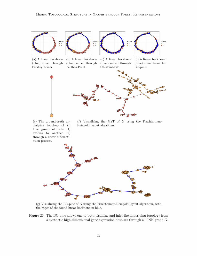
Mining Topological Structure in Graphs through Forest Representations
(a) A linear backbone(blue) mined throughFacilitySteiner.
(b) A linear backbone(blue) mined throughFarthestPoint.
(c) A linear backbone(blue) mined throughCLOFinMSF.
(d) A linear backbone(blue) mined from theBC-pine.
(e) The ground-truth un-derlying topology of D.One group of cells (1)evolves to another (2)through a linear differenti-ation process.
(f) Visualizing the MST of G using the Fruchterman-Reingold layout algorithm.
(g) Visualizing the BC-pine of G using the Fruchterman-Reingold layout algorithm, withthe edges of the found linear backbone in blue.
Figure 21: The BC-pine allows one to both visualize and infer the underlying topology froma synthetic high-dimensional gene expression data set through a 10NN graph G.
37

Vandaele, Saeys, and De Bie
(a) A bifurcating backbone (blue) is mined from theBC-pine (black edges) constructed from a 5NN graphG (grey edges) of real gene expression data D.
(b) The ground-truth underlyingtopology of D.
(c) Visualizing the MST of G using the Fruchterman-Reingold layout algorithm.
(d) Visualizing the BC-pine of G using the Fruchterman-Reingold layout algorithm, withthe edges of the found bifurcating backbone in blue.
Figure 22: The BC-pine allows one to both visualize and infer the underlying topology froma real high-dimensional gene expression data set through a 5NN graph G.
38

Mining Topological Structure in Graphs through Forest Representations
(a) A single node backbone (blue) is minedfrom the BC-pine (red edges) constructedfrom a 10NN graph G (grey edges) of realgene expression data D.
(b) A bifurcating backbone (blue) is minedfrom the BC-pine (red edges) constructedfrom a 10NN graph G (grey edges) of a 3-dimensional embedding of D into diffusionmap coordinates.
(c) The ground-truth under-lying topology of D.
(d) Visualizing the MST of G using the Fruchterman-Reingold layout algorithm.
(e) Visualizing the BC-pine of G using the Fruchterman-Reingold layout algorithm, withthe edges of the found bifurcating backbone in blue.
Figure 23: The BC-pine allows one to both visualize and infer the underlying topology froma real high-dimensional gene expression data set through a 10NN graph G.
39

Vandaele, Saeys, and De Bie
3.4 Quantitative Analysis of the Results
As to evaluate the performance of our method, ideally one would have access to a ground-truth underlying graph-structured topology. However, not only is it difficult to assesswhether there exists a homeomorphic mapping from one graph to another (Lapaugh andRivest, 1980), more often than not we do not have access to a ground-truth model.
Nevertheless, in Section 3.4.1 we will introduce general metrics allowing us to supportand interpret our obtained results, which we will summarize in Section 3.4.2.
Furthermore, we will conduct a separate large scale cell trajectory inference experimentin Section 3.4.3. The knowledge of ground-truth topologies as well as the recent developmentof quantitative metrics for comparing different cell trajectory inference tools (Saelens et al.,2019), allows us to objectively measure the performance of our method for this purpose.
3.4.1 Introducing General Quantitative Metrics
We will consider a variety of metrics that allow us to meaningfully interpret how well ourinferred forest-structured backbone B models the underlying topology of a graph G. Wedistinguish between four different properties we want our backbone to satisfy.
Backbone Size. The relative size of B compared to G should be small for a good simpli-fication. Hence, we will consider n%, the percentage of nodes from G still included in theresulting backbone. As there is a direct relation between the original graph, n%, and thepercentage of edges still included in a forest-structured backbone, we will omit the latter.
Goodness of Fit. Though we prefer a simplification that significantly reduces the size of theoriginal graph G, we also want our backbone to be a good approximation of G. Therefore,we consider the metric
R(B) := 1−∑
v∈V (G) dG(v,B)∑v∈V (G) dG(v, CG)
,
where dG(v,B) denotes the distance of v to its closest node in B, and dG(v, CG) denotesthe distance of v to its closest node in the center of G, defined as the union of nodes thathave minimum eccentricity in their respective connected component of G. Inspired by thecoefficient of determination in linear regression, we consider this metric to be a measurefor how much of the ‘variance’ in our graph G is explained by the model B. However, wedo not consider squared distance as in the usual definition of this coefficient, to lessen theeffect of outliers. As we do not assume G to reside in any vector space, there is no definitionof an ‘average’ node. Hence, our notion of ‘mean’ is fulfilled by the ‘center’ in graphs.
Smoothness. We want our backbone B to pass ‘smoothly’ through our graph, insteadof ‘wiggling’ through many nodes (compare to overfitting in linear regression). To thisend, we compute the projection GB of G on B, by connecting each node of G throughits closest path to B. We then compute the ratio σ := dG(u,v)
dGB(u,v) , where u and v are the
most distant nodes in G. Hence, σ(B) denotes how well the distance between the twofurthest points in G is preserved through B. Note that trivially σ(B) = 1 if B was obtainedthrough FarthestPoint. Furthermore, σ is ‘penalized’, i.e., further from 1, when centeringour backbone and preventing it from passing through outliers. However, this is exactlywhat we want.
40

Mining Topological Structure in Graphs through Forest Representations
Commute Time Preservation. One of the most difficult qualities of a forest-structuredbackbone B to assess, is how well it preserves the metric induced by the original graphG. Missing cycles may result in failing to preserve the original metric, whereas in thecase of curvature and outliers, we actually wish to not preserve the original metric as closeas possible. To this end, we consider the correlation coract between the average commutetimes of the original graph G and the projection of G on GB (Fouss et al., 2007). Thesecommute times are based on a Markov-chain model of random walk through the graph,which have shown to effectively deal with outliers in graphs (Moonesignhe and Tan, 2006).Note that however, this metric does not account for the fact that we cannot include cyclesin a forest-structured backbone.
3.4.2 Quantitative Summary of our Results
Table 1 summarizes the settings in terms of leaves we used to obtain the backbones for thegraphs discussed in Section 3.3 through our method. Each of our baselines also requires anumber of nodes to be selected per component, for which we used the kcomp-row of Table 1.
SR K HP GoT NeurIPS KDD EQ SC RC1 RC2
kmax 10 10 50
kspec 10 5 5 35
kcomp 2 2 2-2-0 8-2 5 5 35 2 3 3
Table 1: Input and output summary to obtain a forest-structured backbone through BCB.kmax: upper bound on the total number of leaves for solving CLOF to increaseefficiency (blank if not specified). kspec: the specified number of leaves to beselected once the subforest had been fully grown or up until the maximum numberof leaves (blank if estimated through minimizing second-order finite differences).kcomp: the number of resulting leaves for each connected component (0 meaninga backbone component consisting of one node).
Table 2 summarizes the network sizes for each graph G (n = |V (G)|, m = |E(G)|),runtimes, and our quantitative results for the metrics introduced in Section 3.4.1. All theseresults were obtained using non-optimized R code on a machine equipped with an Intel R©
CoreTM i7 processor at 2.6GHz and 8GB of RAM. Note that the specified runtimes in Table2 for our method are those when given the (possibly infinite) upper bounds kmax from Table1. The runtimes for the baselines are those when specified to exactly select kcomp nodes.We observe that our method scales well to graphs with thousands of nodes. We will discussfurther directions for scaling our method to higher order graphs in Section 5.
Our method also scales well according to the topological complexity, whether given orbounded by a number of leaves. In contrast, FacilitySteiner is significantly slower whenselecting more medoids in higher order graphs, taking 8.6min for the earthquakes data.Since the placement of medoids through FacilitySteiner is density based, it also strugglesto identify important regions that make up the topology, even when specified to select thecorrect number of nodes to do so (Figure 2a). Clear examples of this are the bifurcating realcell trajectory data sets, for which FacilitySteiner infers a linear trajectory. Furthermore,
41

Vandaele, Saeys, and De Bie
time n% R σ coract kcomp
Swiss Roll (SR)FacilitySteiner 4.19s 1.0% 0.69 0.997 0.48 2
n = 1000FartherstPoint 4.71s 2.1% 0.88 1 0.49 2
m = 47 013CLOFinMSF 2.66s 28% 0.93 0.62 0.16 2
ClOFinBC-pine 3.41s 2.3% 0.89 0.97 0.49 2
Karate (K)FacilitySteiner 0.046s 12% 0.40 1 0.35 2
n = 34FarthestPoint 0.005s 21% 0.48 1 0.36 2
m = 78CLOFinMSF 0.31s 26% 0.54 0.90 0.39 2
ClOFinBC-pine 0.018s 12% 0.44 0.95 0.39 2
Harry Potter (HP)FacilitySteiner 0.029s 10% 0.50 1 0.96 2-2-0
n = 63FarthestPoint 0.007s 16% 0.53 1 0.96 2-2-0
m = 221CLOFinMSF 0.067s 16% 0.53 1 0.96 2-2-0
ClOFinLCC-pine 0.23s 21% 0.56 1 0.96 2-2-0
GoTFacilitySteiner 0.22s 17% 0.72 1 0.93 7-2
n = 208FarthestPoint 0.026s 29% 0.76 1 0.90 8-2
m = 326CLOFinMSF 0.13s 26% 0.78 0.95 0.90 8-2
ClOFinLCC-pine 0.40s 29% 0.81 1 0.91 8-2
KDDFacilitySteiner 20s 0.19% 0.22 0.94 0.13 3
n = 5747FarthestPoint 11s 0.77% 0.21 1 0.14 5
m = 19 751CLOFinMSF 4.5s 3.3% 0.32 0.55 0.12 5
ClOFinBC-pine 32s 0.87% 0.31 0.87 0.16 5
NeurIPSFacilitySteiner 20s 0.19% 0.14 1 0.15 3
n = 6252FarthestPoint 12s 0.72% 0.18 1 0.16 5
m = 15 770CLOFinMSF 5s 1.9% 0.23 0.95 0.12 5
ClOFinBC-pine 30s 0.88% 0.26 0.84 0.14 5
Earthquakes (EQ)FacilitySteiner 8.6min 8.4% 0.96 0.81 0.56 23
n = 5000FarthestPoint 14s 9.6% 0.97 1 0.59 26
m = 31 146CLOFinMSF 14s 54% 0.99 0.69 0.28 35
ClOFinBC-pine 24s 16% 0.99 0.79 0.58 35
Synth. cells (SC)FacilitySteiner 0.16s 1.6% 0.59 0.9994 0.52 2
n = 556FarthestPoint 0.14s 2.2% 0.59 1 0.48 2
m = 4636CLOFinMSF 0.034s 7.9% 0.82 0.56 0.50 2
ClOFinBC-pine 0.49s 5.2% 0.81 0.53 0.65 2
Real cells 1 (RC1)FacilitySteiner 0.073s 2.3% 0.50 1 0.67 2
n = 355FarthestPoint 0.05s 4.2% 0.59 1 0.68 3
m = 1543CLOFinMSF 0.052s 9.6% 0.67 0.52 0.64 3
ClOFinBC-pine 0.15s 5.4% 0.64 0.78 0.67 3
Real cells 2 (RC2)FacilitySteiner 0.048s 6.5% 0.60 1 0.67 2
n = 154FarthestPoint 0.017s 11% 0.67 1 0.69 3
m = 974CLOFinMSF 0.029s 34% 0.83 0.60 0.46 3
ClOFinBC-pine 0.38s 11% 0.73 0.81 0.68 3
Table 2: Quantitative summary of our experimental results. Our newly introduced methodfor mining backbones in graphs through forest representations is marked in blue.
42

Mining Topological Structure in Graphs through Forest Representations
unlike FarthestPoint and the backbones constructed through CLOF, there is no straight-forward way to extract the result for a lower number of selections through the output ofFacilitySteiner. One needs to rerun the entire algorithm for this, making it difficult to tunethe resulting topological complexity through FacilitySteiner.
Overall, not a single metric is able to fully quantify the global performance of eachmethod on its own. Note that we did not mark ‘winning’ values, as extremes may alsoindicate a bad performance (e.g., σ is always 1 for FarthestPoint). However, we note thatthese metrics strongly support our observations up until now. E.g, CLOFinMSF oftenresults in the best approximation of the original graph (high R), at the cost of includingmany more nodes (high n%), and ‘wiggling’ through all of them (low σ). In contrast, ourmethod provides a backbone that approximates the original graph nearly as well (sometimeseven better), using much fewer nodes in order to do so. This is most notably the case withthe Swiss Roll (n% = 2.3%, R = 0.89 with our method vs. n% = 28%, R = 0.93 withCLOFinMSF), the KDD network (n% = 0.87%, R = 0.31 vs. n% = 3.3%, R = 0.32),the NeurIPS network (n% = 0.88%, R = 0.26 vs. n% = 1.9% and R = 0.23), and theearthquakes (n% = 16%, R = 0.99 vs. n% = 54%, R = 0.99). Our method also resultsin a consistent smoothing for the co-authorship graphs, unlike CLOFinMSF (respectively,σ = 0.87 (KDD), σ = 0.84 (NeurIPS) vs. σ = 0.55 (KDD), σ = 0.95 (NeurIPS)).
FacilitySteiner and FarthestPoint often result in smaller (low n%) and smoother (highσ) backbones, however, at the cost of providing worse approximations (low R) of the originalgraphs. This can be either due to failing to span the entire graph (FacilitySteiner), or failingto center the resulting backbone in the graph (FarthestPoint).
All methods perform similarly well in terms of preserving the average commute times.The most notable exceptions are where either CLOFinMSF performs worse, such as theSwiss Roll (coract = 0.49 with our method vs. coract = 0.16 with CLOFinMSF), the earth-quakes (coract = 0.58 vs. coract = 0.28), and the second real gene expression data set(coract = 0.68 vs. coract = 0.46), or where our method performs better, i.e., for the syn-thetic cells (coract = 0.65 vs. a maximum of 0.52 for the other methods).
The main networks contradicting the observations above, are the unweighted networks(HP & GoT). Here, our method actually results in the best approximation of the originalgraph (R equals 0.56 and 0.81, respectively), while remaining a smooth approximation (σequals 1 twice) that well preserves the average commute times (coract equals 0.96 and 0.91,respectively). Furthermore, our method appears to provide the least smooth approximationfor the synthetic cell trajectory data set at first sight (σ = 0.53). However, through Figures21a-21d, we have shown that our method was the only method capable of identifying the trueunderlying topology. The longest shortest path in the original graph—used for computingσ—incorrectly connects the two underlying leaves (Figure 21b), which explains this result.
3.4.3 Large Scale Cell Trajectory Inference
The results we obtained through our newly introduced method, in this section abbreviatedto BCB (Boundary Coefficients to Backbone), on the cell trajectory data sets in Section3.3, lead to a new cell trajectory inference method.
1. start from a (high-dimensional) gene expression data set D;2. use a dimensionality reduction method to reduce the (high-dimensional) noise in D;
43

Vandaele, Saeys, and De Bie
3. construct a kNN graph G from the lower dimensional representation of D;4. construct the BC-pine in G;5. identify the underlying topology from the pine by means of (4).Contrary to many of the existing cell trajectory inference tools (Saelens et al., 2019),
we do not require the data to be represented in a vector space, can infer more complextopologies than linear, bifurcating, or connected ones, and do not preprocess the datathrough a clustering method.
Each of our 333 considered data sets described in Section 3.1 was embedded in a 20-dimensional space using diffusion maps with Pearson correlations and standard settings inR. Consecutively, we estimated the intrinsic dimension d, 3 ≤ d ≤ 20, of our data usingan inference method based on the eigen-multipliers of the embedding. We implementedthe same inference method as the wrapper for Slingshot developed by Saelens et al. (2019).The code for this wrapper can be found on https://github.com/dynverse. We evaluatedour method over multiple values k ∈ {5, 10, 15, 20, 25} for building kNN graphs from ourdiffusion coordinates, using the Euclidean distance between points. The resulting proximitygraph was used to construct a BC-pine, from which we mined the underlying topology usingCLOF. A number of leaves l, 2 ≤ l ≤ 30, was estimated for each connected component inour BC-pine, by minimizing the second-order finite differences of the function mapping thenumber of leaves to the corresponding vertex betweenness cost, as discussed in Section 2.4.2.
We used the four metrics suggested in Saelens et al. (2019) to quantify the quality of ourinferred trajectories, which we summarize below. For full details on the exact computationof these metrics, we refer to Saelens et al. (2019).
• The correlation between geodesic distances, measuring if the positioning of cells issimilar in the ground-truth and inferred trajectory.
• The Hamming-Ipsen-Mikhailov (HIM) metric, measuring the similarity of the weightedadjacency matrices of the ground-truth and inferred trajectory.
• The F1 score between branch assignments, measuring the similarity between the as-signment to branches in the ground-truth and inferred trajectory.
• The correlation between important features, measuring if the same differentially ex-pressed features are found in both the ground-truth and inferred trajectory.
All these metrics lie within [0, 1]. Higher values correspond to better performances. Wealso evaluated the computational cost of our approach in terms of runtime (in seconds) andstorage (in GB). Figure 24 visualizes the performance for each considered metric, as well asfor various choices of k(NN graphs), through cumulative distribution plots.
We first note that the overall performance of our cell trajectory inference method isstable when it comes to the choice of k. In terms of the obtained results, our method turnsout to be comparable to Slingshot. We especially note an increase in performance whenit comes to the correlation between geodesic distances. Furthermore, our method scales atleast as well as Slingshot in terms of runtime, which is mostly affected by the choice of k,i.e., the density of H2(D) (Theorem 8). In terms of storage, our method does scale worse.However, it turns out this is due to computing and storing the entire Pearson correlationmatrix for the embedding. Given the dimensionality reduction, our method scales better in
44
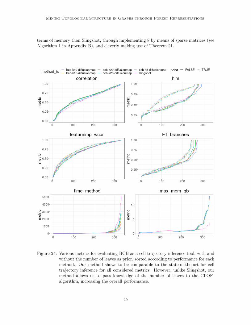
Mining Topological Structure in Graphs through Forest Representations
terms of memory than Slingshot, through implementing 8 by means of sparse matrices (seeAlgorithm 1 in Appendix B), and cleverly making use of Theorem 21.
Figure 24: Various metrics for evaluating BCB as a cell trajectory inference tool, with andwithout the number of leaves as prior, sorted according to performance for eachmethod. Our method shows to be comparable to the state-of-the-art for celltrajectory inference for all considered metrics. However, unlike Slingshot, ourmethod allows us to pass knowledge of the number of leaves to the CLOF-algorithm, increasing the overall performance.
45
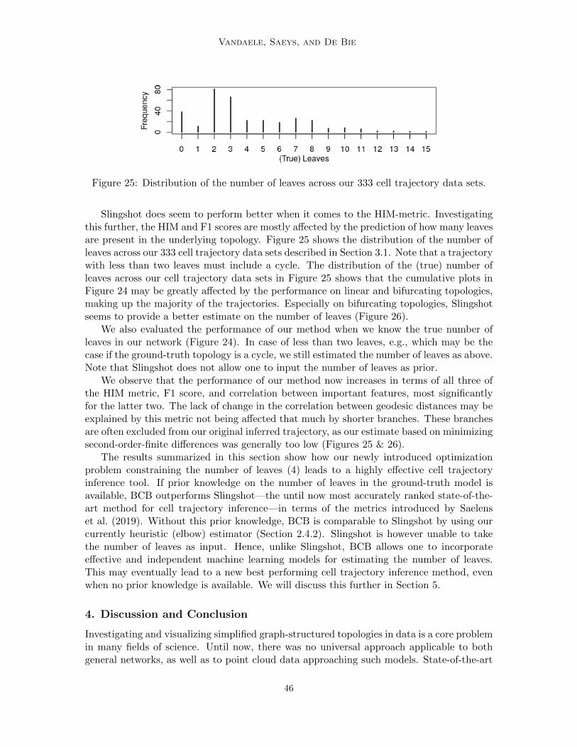
Vandaele, Saeys, and De Bie
Figure 25: Distribution of the number of leaves across our 333 cell trajectory data sets.
Slingshot does seem to perform better when it comes to the HIM-metric. Investigatingthis further, the HIM and F1 scores are mostly affected by the prediction of how many leavesare present in the underlying topology. Figure 25 shows the distribution of the number ofleaves across our 333 cell trajectory data sets described in Section 3.1. Note that a trajectorywith less than two leaves must include a cycle. The distribution of the (true) number ofleaves across our cell trajectory data sets in Figure 25 shows that the cumulative plots inFigure 24 may be greatly affected by the performance on linear and bifurcating topologies,making up the majority of the trajectories. Especially on bifurcating topologies, Slingshotseems to provide a better estimate on the number of leaves (Figure 26).
We also evaluated the performance of our method when we know the true number ofleaves in our network (Figure 24). In case of less than two leaves, e.g., which may be thecase if the ground-truth topology is a cycle, we still estimated the number of leaves as above.Note that Slingshot does not allow one to input the number of leaves as prior.
We observe that the performance of our method now increases in terms of all three ofthe HIM metric, F1 score, and correlation between important features, most significantlyfor the latter two. The lack of change in the correlation between geodesic distances may beexplained by this metric not being affected that much by shorter branches. These branchesare often excluded from our original inferred trajectory, as our estimate based on minimizingsecond-order-finite differences was generally too low (Figures 25 & 26).
The results summarized in this section show how our newly introduced optimizationproblem constraining the number of leaves (4) leads to a highly effective cell trajectoryinference tool. If prior knowledge on the number of leaves in the ground-truth model isavailable, BCB outperforms Slingshot—the until now most accurately ranked state-of-the-art method for cell trajectory inference—in terms of the metrics introduced by Saelenset al. (2019). Without this prior knowledge, BCB is comparable to Slingshot by using ourcurrently heuristic (elbow) estimator (Section 2.4.2). Slingshot is however unable to takethe number of leaves as input. Hence, unlike Slingshot, BCB allows one to incorporateeffective and independent machine learning models for estimating the number of leaves.This may eventually lead to a new best performing cell trajectory inference method, evenwhen no prior knowledge is available. We will discuss this further in Section 5.
4. Discussion and Conclusion
Investigating and visualizing simplified graph-structured topologies in data is a core problemin many fields of science. Until now, there was no universal approach applicable to bothgeneral networks, as well as to point cloud data approaching such models. State-of-the-art
46

Mining Topological Structure in Graphs through Forest Representations
Figure 26: Normalized confusion matrices showing the true vs. the predicted number ofleaves. Note that all methods output a trajectory with at least two leaves. Inthe case of 11 gene expression data sets, the number of neighbors k = 5 was toolow to represent the connectedness of the true model through a neighborhoodgraph, resulting in fragmented backbones with many leaves (ranging from 17 to104). These predictions were discarded from the corresponding confusion matrixfor visualization purposes.
47

Vandaele, Saeys, and De Bie
methods that focused on either one of them were computationally inefficient, sensitive toparameters, noise and outliers, were topologically biased, or did not generalize well. Wesolved these issues by introducing a simple but crucial intermediate step that showed to behighly beneficial throughout this entire paper. That is, designing a forest representationfrom which we may efficiently, robustly, and meaningfully mine topological substructures.
We introduced the boundary coefficient (BC), a coefficient that locates core topologicalstructures well in many complex graphs (Vandaele et al., 2019b). Contrary to existingvertex measures, this coefficient is specifically designed for this purpose. Hence, the BCovercomes many difficulties faced with when dealing with this problem, such as applicabilityto complete networks, robustness to outliers, and the ability to deal with non-uniformbranch lengths and curvature. Along with this, we provided extensive theoretical resultsconcerning the computation of the BC, its robustness, as well as its relation to the ordinarylocal cluster coefficient. We showed that together, the BC and our introduced conceptof f -pines (Vandaele et al., 2019b), provide effective forest representations in which manyconcepts of graph theory, such as longest paths and betweenness centrality, become bothefficiently computable, and topologically meaningful.
Our newly introduced graph-optimization problem under the name of ConstrainedLeaves Optimal subForest (CLOF) is already interesting on a purely theoretical level.CLOF induces a nontrivial monotone submodular set function maximization problem sub-ject to a cardinality constraint on tree graphs, for which a greedy approach provides anexact solution in polynomial time. Nevertheless, we also thoroughly illustrated the impor-tance of this problem, as well as the effectiveness of its solution, for mining substructuresthrough forest representations. All together, we provided a new method for topological dataanalysis of graph-structured data. We qualitatively and quantitatively demonstrated thatour method leads to effective graph-structured models—balancing their size, goodness offit, smoothness, and average commute time preservation—in many types of synthetic andreal world data sets. These may be given weighted or unweighted graphs, point cloud datasets embedded in (non-)Euclidean metric spaces, or high-dimensional data sets.
Naturally, there is no single best method when it comes to extracting the backbone froma network. There will be cases where our approach will not be the best one as well. Examplesare when the connectedness of our graph does coincide with the connectedness of its model,or in case of metric data, when the used proximity graph is not a truthful representationof the underlying model (Figure 23a). Nevertheless, our results convincingly show that weprovided a very promising method across a broad spectrum of realistic applications.
5. Further Work
Scalability. Our method shows to scale well to thousands of nodes. At first sight, this maynot be enough for many practical applications, such as large network embedding (Tanget al., 2015; Chen et al., 2018). Nevertheless, there are many practical examples, such ascell trajectory data, where identifying the underlying topology for graphs of this order re-mains an important problem. Furthermore, our method may scale to larger order graphsby optimizing or even parallelizing our current implementation to compute boundary co-efficients, the most expensive part of our method. Algorithms for approximating these
48

Mining Topological Structure in Graphs through Forest Representations
coefficients may be investigated on a theoretical, probabilistic, and experimental level aswell.
Generalization. One may increase the local scope of the boundary coefficient. I.e., the BCcurrently only averages over pairs of neighbors, but it may as well consider neighbors ofneighbors, and so on. In this way, we may be able to effectively mine topological skeletonsin non graph-structured data with a locally higher intrinsic dimension. An example of thiswould be the Swiss Roll from Section 3, where we increase the width of the manifold (alongthe z-axis), while also increasing the sparsity of the proximity graph.
We experimentally demonstrated that modeling our topology through a (sub)forest isnot a severe limitation when it comes to cycles. These may be more efficiently discoveredthrough persistent homology if our backbone provides a significant size reduction, whileremaining spread out across the underlying topology. However, we have yet to provide aneffective method for ‘lifting’ the holes found by means of topological persistence to our forest-structured backbone, i.e., closing the gaps corresponding to these holes. Persistent homologyhas also been connected to minimum spanning trees and their higher-dimensional analoguesof minimum spanning acycles on a theoretical level (Kalisnik et al., 2019). Connecting theseresults to CLOF may lead to new theoretically well-founded approximation algorithms forcomputing persistence (Silva and Carlsson, 2004; Oudot, 2015).
Another interesting direction is to investigate how our method generalizes to directedgraphs. From a topological viewpoint, (anti-)arborescences could be very useful to interpretas possible backbone structures in directed graphs, as they have a natural and consistent flowdefined on them. However, this may already become too restrictive. Unlike for unweightedgraphs, such backbones may become non-existing if we require that each other node in thegraph can be connected in some way to this backbone, through either a fixed or varyingdirectionality. Furthermore, the BC may become undefined for nodes in weakly connectedcomponents, that are not strongly connected, and a different core measure may be moreappropriate. This leads to many new theoretical and practical research questions.
Cell Trajectory Inference. In the case of cell trajectory inference, we noted that even thebest performing cell trajectory methods, according to Saelens et al. (2019), often strugglein correctly identifying the backbone, including its number of leaves (Figures 24 & 26).Empirical investigation shows that for many data sets, branches are difficult to separatefrom each other due to a high amount of noise (even after a dimensionality reduction),or that branches which are relatively short according to some main trajectory are leftundetected (intuitively, our ‘elbow’ in Figure 10b will occur too soon). However, we showedhow that our method may highly benefit from a more effective leaf inference method forthis purpose, as it can use this knowledge to increase its performance. A possible approachis to include a topological inference method. Carlsson (2014) presented a method underthe name of functional persistence, that allows one to deduce ‘flare’-like structures. Thesemay be used to distinguish between a Y-shape and an X-shape (but not between an X-shape and an H-shape). In this way, we are able to construct topological summaries, i.e.,persistence diagrams summarizing topological features of data sets, that have recently leadto effective topological inference and classification tools (Rieck and Leitte, 2017; Hofer et al.,2017; Rieck et al., 2019), which may aid us in quantifying or learning the number of leavesindependent of our used method.
49

Vandaele, Saeys, and De Bie
Applications. We only focused on applications within the field of topological data analysisthroughout this paper. Correctly identifying the graph-structured model is the exact pur-pose of cell trajectory inference methods. For other graphs such as social networks, we alsoshowed that we can meaningfully identify backbone structures, both on a qualitative andquantitative level. Our procedure provides a way to visualize or obtain insight into theirunderlying structure. Nevertheless, this is often not the end goal for these networks. Hence,a wide variety of new applications of backbones, such as community detection, subgroupdiscovery, and graph embeddings, is yet to be discovered. E.g., Chen et al. (2018) intro-duced a heuristic algorithm to iteratively simplify a graph, as to increase the performanceof any existing graph embedding method through better initializations. Hence, initializingthe embedding through a well-chosen backbone can lead to a graph embedding method thatrespects topological properties of the graph.
Finally, one may investigate how backbone extraction improves existing models forgraph-structured data, and vice versa. E.g., graph convolutional networks (GCNs) haverecently led to many new applications for graphs (Kipf and Welling, 2016a). On the onehand, prior knowledge of nodes near or on the core structure of the graph may enhance theability to learn from graphs through better initializing a GCN. This is similar to the methoddescribed above for improving graph embeddings, which is also one of the many applicationsof GCNs. On the other hand, similar to how an initial dimensionality reduction improvesthe performance of cell trajectory inference, graph autoencoders (Kipf and Welling, 2016b)may serve as a tool to find a latent or denoised representation of the graph, prior to thefinal backbone extraction.
Acknowledgments
The research leading to these results has received funding from the European ResearchCouncil under the European Union’s Seventh Framework Programme (FP7/2007-2013) /ERC Grant Agreement no. 615517, from the Flemish Government under the “Onderzoek-sprogramma Artificiele Intelligentie (AI) Vlaanderen” programme, from the FWO (projectno. G091017N, G0F9816N, 3G042220), and from the European Union’s Horizon 2020 re-search and innovation programme and the FWO under the Marie Sklodowska-Curie GrantAgreement no. 665501.
We furthermore acknowledge Bo Kang and Bastian Rieck for helpful discussions, aswell as Wouter Saelens and Robrecht Cannoodt for helping us setting up our large-scalecell trajectory inference experiments. Finally, we thank the anomynous reviewers for theirmany insightful comments and suggestions that had a noticeable positive impact on boththe content and presentation of our work
Appendix A. Supplementary Experiments
In this section, we provide further analysis of our method, by qualitatively discussing ourobtained backbones for two of the graphs discussed in Section 3.
Game of Thrones Network. Figure A.1 shows the original Game of Thrones Network G, anLCC-pine in G, a forest-structured backbone B mined from this LCC-pine, and the union
50

Mining Topological Structure in Graphs through Forest Representations
of the representative cycles for the two most persistent holes obtained through persistenthomology of (V (B), dG). Nodes are colored according to their ground-truth community,i.e., the family they belong to.
We obtained a backbone B with 10 leaves using ‘standardized’ vertex betweenness as costfunction. I.e., the betweenness for each node was divided by the total cost of its correspond-ing connected component. Note that the cost of the smaller component in the backboneis relatively low according to its sum of (original) betweenness centralities, as it containsmuch fewer nodes than the larger component. Using non-standardized betweenness, onewould either need to further increase the number of leaves for the smaller component to berepresented in the backbone, or manually specify the number of leaves for each component.
Our backbone B illustrates well how the ground-truth communities make up the entiretopology of our graph. E.g., there is a branch corresponding to House Tyrell, to HouseGreyjoy, to House Martell, to House Targaryen, . . . . Not only is the backbone able toseparate the communities well, but it also is able to infer how different communities areconnected. E.g, House Stark, House Lannister, the Boltons and further on House Frey, areall connected through Sansa Stark. Eddark Stark (often referred to as Ned Stark), connectsSansa Stark (and through her the Lannisters, Boltons, and House Frey) to a branch of‘older’ Starks, to House Tully, and to House Targaryen through Jon Snow.
Nevertheless, there are again some obvious ‘gaps’ in our backbone representation Bof G. E.g., Sansa Stark immediately connects to a branch of Lannisters through TyrionLannister, but to reach the other cluster of Lannisters, she must first travel through theBoltons, and then through House Frey, making it apparent that these groups of Lannistersform seperated communities. Another obvious gap is present in House Baratheon, as wefirst need to travel through House Lannister, House Stark, and House Targaryen beforereconnecting this community. Though some smaller gaps seem to be present as well (andmay also be identified using persistent homology), the ones discussed above correspond tothe two most persistent holes one obtains by computing persistent homology of the metricspace (V (B), dG) (Section 2.4.3). The union of the two corresponding representative cyclesare shown in Figure A.1 as well. Note that these cycles overlap through a path betweenJaime Lannister and Sansa Stark.
NeurIPS Co-authorship Network. We again applied our method to construct a tree-structuredbackbone with 5 leaves. The resulting tree graph is shown in Figure A.2.
As we did for the KDD network, we verified that the cores of our tree representations,i.e., the BC-pines, indeed correspond to meaningful core structures (Figure A.3). We observethat our method provides consistent results, as again, the BC-pine retract towards a corestructure marking authors with a high number of citations, and who have been present veryearly in the considered conference.
Appendix B. Algorithms and Computational Costs
In this section, we analyze the computational cost and provide basic pseudocode for thealgorithms used in our method for topological data analysis of graph-structured data sets.
51

Vandaele, Saeys, and De Bie
Figure A.1: A forest-structured backbone with 10 leaves (red edges) mined from the LCC-pine constructed from the Game of Thrones network (grey edges). Nodes arecolored according to their ground-truth community, i.e., the House they belongto. White nodes correspond to members that are unassigned to any house.Persistent homology of the metric space induced by the original metric in G onthe nodes of the backbone is used to identify cycles missing in the backbone(orange edges).
52

Mining Topological Structure in Graphs through Forest Representations
Figure A.2: A tree-structured backbone for the NeurIPS co-authorship network with 5leaves. Nodes and edges are colored according to their closeness to one ofthe 6 branches.
Figure A.3: Various measures after iteratively pruning the regular MST (red), the FPS tree(green), and the BC-pine (blue), for the NeurIPS network. (Left) Fraction oforiginal graph size. (Middle) Average number of (NeurIPS) citations. (Right)Average year of first published (NeurIPS) paper.
53

Vandaele, Saeys, and De Bie
Input: weighted graph GOutput: vector of boundary coefficients BC
1 hop1 = spam(hop k approx(G, k=1)) #compute hop-1-approximation2 hop2 = spam(hop k approx(G, k=2)) #compute hop-2-approximation3 BC = (apply.spam(hop1, 1, sum) * apply.spam((1 / hop1), 1, sum)
- diag((1 / hop1) %*% hop2ˆ2 %*% (1 / hop1)) / 2) / (degree(G)ˆ2)#compute boundary coefficients
4 return(BC)Algorithm 1: Computing the boundary coefficients through sparse matrices. ‘spam’converts matrices to sparse matrix format. ‘apply.spam(A, 1, f)’ applies the functionf to each row of the sparse matrix A. The operations ‘*’ and ‘ˆ2’ denote element-wise multiplication, whereas ‘%*%’ denotes matrix multiplication. ‘1 / A’ returns theelement-wise inverse of a sparse matrix A. ‘diag(A)’ returns the diagonal of matrix A.
Theorem B.1 Let G be an undirected, positively weighted graph, with n nodes and m edges.The boundary coefficients of all nodes in V can be determined in O(n(m+n1.374)) time usingAlgorithm 1.
Proof Obtaining the hop-k-approximations can be done O(n(m + n log n)) time throughDijkstra’s algorithm. The matrix operations can be done in O(n2.374) time, which is thecomputational cost of matrix multiplication (Davie and Stothers, 2013).
Remark B.2 The computational cost stated in Theorem B.1 is worst-case, since it doesnot account for the sparsity of Hk(D), k ∈ {1, 2}. In practice, we note that working withsparse matrices significantly improves the efficiency of computing the boundary coefficients.
Theorem B.3 Let G be a graph with n nodes and m edges, and f : V → R. Then anf -pine of G can be determined in O(α(m,n)m) time using Algorithm 2. Here α is theclassical functional inverse of the Ackermann function, which for all practical purposes maybe considered a constant no greater than 4 (Sundblad, 1971).
Proof The stated complexity is that of computing the regular minimum spanning forest(Chazelle, 2000). Reweighing the edges can be done in O(m) time.
Theorem B.4 Let T = (V,E) be a tree graph with n nodes (and n − 1 edges), and f areal-valued function associating a positive cost to either each vertex or each edge of T . Then
Input: graph G, vertex-valued cost function f on GOutput: an f -pine of G
1 return(mst(G, weights=f [E(G)[,1]] + f [E(G)[,2]]))Algorithm 2: Computing the f -pine. ‘mst’ is a function that computes the minimumspanning of a graph. The used weights follow from the result in Proposition 13.
54
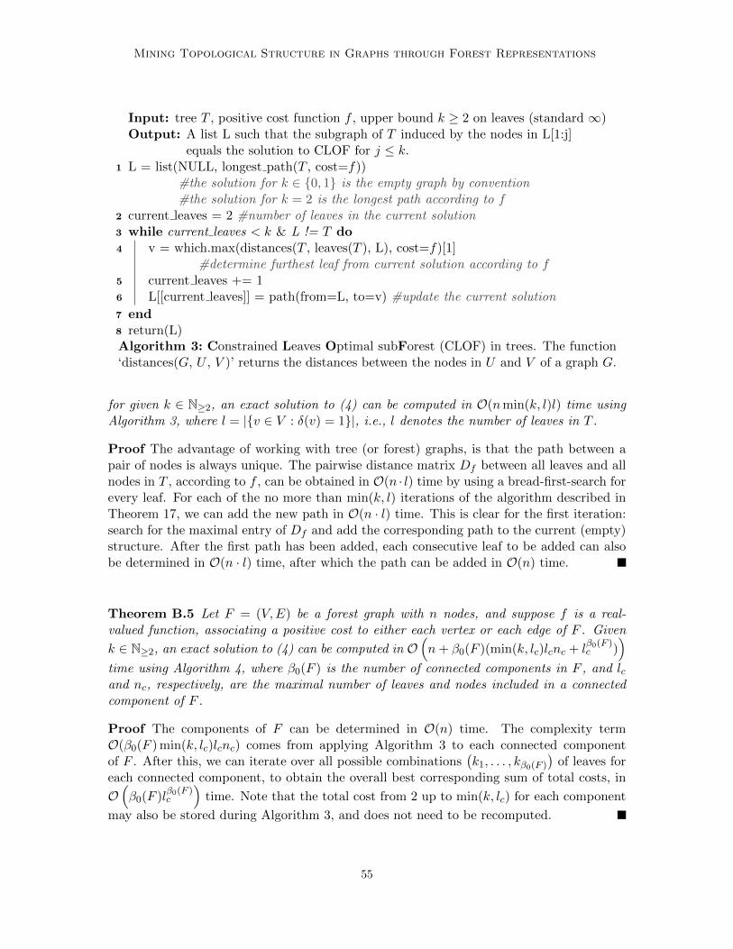
Mining Topological Structure in Graphs through Forest Representations
Input: tree T , positive cost function f , upper bound k ≥ 2 on leaves (standard ∞)Output: A list L such that the subgraph of T induced by the nodes in L[1:j]
equals the solution to CLOF for j ≤ k.1 L = list(NULL, longest path(T , cost=f))
#the solution for k ∈ {0, 1} is the empty graph by convention#the solution for k = 2 is the longest path according to f
2 current leaves = 2 #number of leaves in the current solution3 while current leaves < k & L != T do4 v = which.max(distances(T , leaves(T ), L), cost=f)[1]
#determine furthest leaf from current solution according to f5 current leaves += 16 L[[current leaves]] = path(from=L, to=v) #update the current solution
7 end8 return(L)Algorithm 3: Constrained Leaves Optimal subForest (CLOF) in trees. The function‘distances(G, U , V )’ returns the distances between the nodes in U and V of a graph G.
for given k ∈ N≥2, an exact solution to (4) can be computed in O(nmin(k, l)l) time usingAlgorithm 3, where l = |{v ∈ V : δ(v) = 1}|, i.e., l denotes the number of leaves in T .
Proof The advantage of working with tree (or forest) graphs, is that the path between apair of nodes is always unique. The pairwise distance matrix Df between all leaves and allnodes in T , according to f , can be obtained in O(n · l) time by using a bread-first-search forevery leaf. For each of the no more than min(k, l) iterations of the algorithm described inTheorem 17, we can add the new path in O(n · l) time. This is clear for the first iteration:search for the maximal entry of Df and add the corresponding path to the current (empty)structure. After the first path has been added, each consecutive leaf to be added can alsobe determined in O(n · l) time, after which the path can be added in O(n) time.
Theorem B.5 Let F = (V,E) be a forest graph with n nodes, and suppose f is a real-valued function, associating a positive cost to either each vertex or each edge of F . Given
k ∈ N≥2, an exact solution to (4) can be computed in O(n+ β0(F )(min(k, lc)lcnc + l
β0(F )c )
)time using Algorithm 4, where β0(F ) is the number of connected components in F , and lcand nc, respectively, are the maximal number of leaves and nodes included in a connectedcomponent of F .
Proof The components of F can be determined in O(n) time. The complexity termO(β0(F ) min(k, lc)lcnc) comes from applying Algorithm 3 to each connected componentof F . After this, we can iterate over all possible combinations
(k1, . . . , kβ0(F )
)of leaves for
each connected component, to obtain the overall best corresponding sum of total costs, in
O(β0(F )l
β0(F )c
)time. Note that the total cost from 2 up to min(k, lc) for each component
may also be stored during Algorithm 3, and does not need to be recomputed.
55

Vandaele, Saeys, and De Bie
Input: forest F , positive cost function f , number of leaves k.Output: A subgraph of F corresponding to the solution of CLOF.
1 treeSols = lapply(components(F ), function(T) Algorithm3(T, f , k))#apply Algorithm 3 to each connected component of F#return a list of all solutions (note that each solution is a list itself)
2 currentCost = -Inf #cost of the current best solution in F3 for 0 ≤ l1, . . . , lβ0(F ) ≤ k do
4 if(sum(l1, . . . , lβ0(F )) > k) continue #skip if total number of leaves is > k
5 thisCost = sum(cost(treeSols[[1]][1:l1]), . . . , cost(treeSols[[β0(G)]][1:lβ0(F )]))#evaluate the cost of the current potential solution according to f#the cost of each subtree can be stored during the execution#of Algorithm 3 for fast evaluation
6 if thisCost > currentCost then7 currentCost = thisCost8 bestSol = subgraph(F , c(treeSols[[1]][1:l1], . . . , treeSols[[β0(F )]][1:lβ0(F )]))
#update the current optimal solution#the solution is determined as the subgraph in F#induced by all partial solutions
9 end
10 end11 return(bestSol)
Algorithm 4: Constrained Leaves Optimal subForest (CLOF) in forests.
The additional exponential complexity term shows to be negligible in practice: oftenβ0(F ) is 1 or small. Theorem 21 allows us to significantly reduce lc in practice as well.
Appendix C. Other Cost Functions for CLOF
In Section 2.4.1, we demonstrated the usefulness of betweenness centrality as vertex-valuedcost function g used for identifying a subforest by means of (4) for the purpose of topologicaldata analysis of graph-structured data. Here, we discuss some other interesting choices.
The original edge weights. As our backbone is meant to span the entire underlying topologyof our given graph seen as a (shortest path) metric space, we may consider a longest ormultiple longest paths in our f -pine to make up the backbone. E.g., the longest path shownin Figure C.4a identifies the correct underlying model, apart from the location of its leaves,chosen to be the furthest points in the local noise around the true leaves.
In terms of performance, this method is affected by the presence of outliers. E.g., thelinear backbone in the pine shown in Figure C.4a is of similar length as the path in thepine that takes a turn to pass pass through the centered outlier. Though we got lucky inthis case, we note that such ‘interbranching regions of outliers’ are often present in manypractical examples, such as in cell trajectory data, as discussed by Saelens et al. (2019).
In terms of scalability, note that our f -pine generally has many leaves due to Theorem11. If we take a look at the case where our original graph is connected, i.e., where the f -pineF is a tree graph, then this implies that the number of leaves l in F may be of order n,
56

Mining Topological Structure in Graphs through Forest Representations
(a) Optimal subgraph with 2 leaves in a BC-pine according to the original edge weights(vertices in red). A single edge weight ishowever not representative for whether thecorresponding edge is important for inclusionin the backbone or not, as it is not basedon the resulting f -pine. Using our currentimplementation, the algorithm described inTheorem B.4 takes 56s to execute for theresulting BC-pine with 477 nodes, with noupper bound on k.
(b) Optimal subgraph with 2 leaves in apruned BC-pine according to the vertex de-gree (edges in red). High degree nodes rep-resent important nodes that should be in-cluded in the backbone, according to Theo-rem 21. The algorithm described in TheoremB.4 now takes 0.1s to execute with no upperbound on k, a significant improvement com-pared to using the original edge weights ascost. This illustrates the power of Theorem21 when working with pines.
Figure C.4: Examples of solutions to (4) for cost functions other than vertex betweenness.
where n is the number of nodes in F . If one fully grows the pine by through Algorithm 3,and consequently estimates an appropriate number of leaves k as discussed in Section 2.4.2,Theorem B.4 implies that this computation may be close to cubic in n. Its memory usagewill be close to squared in n, due to storing the pairwise distance matrix between leaves andall other nodes. Hence, apart from often not having a meaningful interpretation (FigureC.4a), allowing the inclusion of any leaf of the pine makes our current implementation forsolving (4) difficult to scale to larger data sets.
The degree of a vertex. By Proposition 11, (locally) high degree nodes represent localminima of f in an f -pine F . Given f is a core measure where low values indicate corenodes, these are exactly the nodes where we want our backbone to pass through. Hence, wemay use the vertex-valued degree function g ≡ δF for optimizing (4). The result for g ≡ δFis less affected by outliers due to their low density in the original graph.
This cost function g is constant on leaves by definition. Hence, we may apply Theorem 21to first prune F , often leading to a significant reduction of the graph size due to Proposition11. In terms of Theorem B.4, this implies that both terms l and n decrease significantly,leading to a much better computation time, as well as storage cost (which is O(l · n)).
Figure C.4b shows the resulting solution of (4) in a pruned BC-pine. High degree nodescorrespond to core nodes in the backbone, but not necessarily conversely. Though extendingthe two leaves of the linear backbone by connecting each one of them to an arbitrarily chosenneighboring leaf results in the optimal solution of (4) in the original pine (Theorem 21), wedo not conduct this step as this will again introduce randomness to the choice of leaves.
57

Vandaele, Saeys, and De Bie
Appendix D. Theorems and Proofs
Proof of Proposition 3 Using the equalities given in (1), we have
BC(v) =12 |{u,w ∈ N (v) : {u,w} ∈ E}| − |{u,w ∈ N (v) : {u,w} /∈ E ∧ u 6= w}|+ δ(v)
δ(v)2.
Since
|{u,w ∈ N (v) : {u,w} /∈ E ∧ u 6= w}| = δ(v)2 − |{u,w ∈ N (v) : {u,w} ∈ E}| − δ(v),
we find
BC(v) =32 |{u,w ∈ N (v) : {u,w} ∈ E}|+ 2δ(v)− δ(v)2
δ(v)2
=δ(v)− 1
δ(v)
(3
2
∑u,w∈N (v) 1{u,w}∈E
δ(v)(δ(v)− 1)
)+
2− δ(v)
δ(v)
=δ(v)− 1
δ(v)
(3
2LCC(v)− 1
)+
1
δ(v).
Note that for graphs G = (V,E) without loops, {u, v} ∈ E =⇒ u 6= v.
Proposition D.6 until Proposition D.9 present the other essential properties of general-izations of the LCC that the BC satisfies (Wang et al., 2017)—apart from its applicabilityto fully weighted networks—as discussed in Section 2.1.3.
Proposition D.6 (Weight-scale invariance, Vandaele et al. (2019b)). Let G = (V,E) bean undirected graph without selfloops, with weighting function ω : E → R+. Let ωλ :E → R : {u, v} 7→ λω({u, v}) for a global scale factor λ > 0. Then for every v ∈ V ,BCλ(v) = BC(v), where BCλ(v) equals the boundary coefficient of v for the new weightingfunction ωλ.
Proof By multiplying each edge weight with a global scale factor λ > 0, the shortest pathdistance between any two nodes is also scaled by the same factor λ. Hence, the statedequality easily follows from Definitions 1 & 2.
Lemma D.7 Let G = (V,E) be an undirected graph, with weighting function ω : E → R+.Suppose that E denotes an additive noise matrix, which defines a new weighting functionωε : E → R+ : {u, v} 7→ ω({u, v}) + Eu,v. Then the following statements are valid:
1. lim‖E‖∞→0 ‖d− dε‖∞ = 0, where d denote the shortest path metric on V according toω, and dε according ωε, where we follow the convention that d(u, v) − dε(u, v) = 0 ifu and v lie in different connected components of G;
2. for any u, v, w ∈ V belonging to the same connected component of G, with u 6= v 6= w,limε→0 Tε(u, v, w) = T (u, v, w), where T (u, v, w) denotes transmissivity of v for u andw according to ω, and Tε(u, v, w) according to ωε.
58

Mining Topological Structure in Graphs through Forest Representations
Proof 1. Suppose u, v ∈ V , and P is a shortest path from u to v according to ω withlength d(u, v). Then the length of the same path P according to ωε is bounded from aboveby d(u, v)+ |E(P )| · ‖E‖∞ ≤ d(u, v)+ |E| · ‖E‖∞, where |E(P )| denotes the number of edgeson P . Since the length of the shortest path from u to v according to ωε is at most thelength of P according to ωε, it holds that dε(u, v) ≤ d(u, v) + |E|‖E‖∞. Analogously, wehave d(u, v) ≤ d(u, v)ε + |E| · ‖E‖∞, so that lim‖E‖∞→0 |dε(u, v)− d(u, v)| = 0. As u and vwere chosen arbitrarily, the stated theorem holds.
2. This easily follows from Proposition D.7.1. and Definition 1.
Proposition D.8 (Continuity). Let G = (V,E) be an undirected graph without selfloops,with weighting function ω : E → R+. Suppose ωε is a new weighting function on E thatdiffers in exactly one edge e ∈ E by an additive constant ε ∈ R, i.e., ωε(e) = ω(e) + ε ∈ R+,and ωε|E\{e} ≡ ω|E\{e}. If BCε denotes the boundary coefficient function according to thenew weighting function ωε, then limε→0BCε(v) = BC(v) for all v ∈ V with δ(v) > 0.
Proof This easily follows from Lemma D.7 and Definition 2.
The problem in the ordinary formulation of the ‘robustness to noise’ property statedby Wang et al. (2017), is that the error-value ∆(E) is not well-defined when a node has aboundary coefficient of 0. Hence, we consider a slight variant below.
Proposition D.9 (Robustness to noise, Vandaele et al. (2019b)). Let G = (V,E) be anundirected graph, with weighting function ω : E → R+. Suppose that E denotes an additivenoise matrix, which defines a new weighting function ωε : E → R+ : {u, v} 7→ ω({u, v}) +Eu,v. If f : R→ R is any continuous function such that f ◦ BC(v) 6= 0 for any v ∈ V , then
∆(E) :=100
|V |∑v∈V
∣∣∣∣f ◦ BCε(v)− f ◦ BC(v)
f ◦ BC(v)
∣∣∣∣ −−−−−→‖E‖∞→00 ,
where BCε(v) equals the boundary coefficient of v for the new weighting function ωε.
Proof This follows from Lemma D.7 and f being continuous.
Remark D.10 The fact that we consider our variant to robustness of noise an equallyimportant property for our method for topological data analysis of graph-structured data,is due to Proposition 12 stating that BC-pines are invariant under affine transformationsof the BC with a positive scaling factor. The BC may always be mapped to an intervalexcluding 0 using such continuous transformation.
Note that the theoretical rate of convergence of ∆(E) in Theorem D.9 depends on |E|(see the proof of Lemma D.7.1.), a consequence of allowing arbitrary long paths (in termsof number of edges) between the endpoints of a triple adjacent to a node, to compute theBC.
The following proposition justifies the naming ‘hop-k-approximation’, introduced in Sec-tion 2.1.4.
59

Vandaele, Saeys, and De Bie
Proposition D.11 Let G = (V,E) be a connected, undirected, positively weighted graph,and D the matrix of pairwise shortest path distances between the nodes of G. Then thefollowing statements are valid:
1. H0(D) = (0)u,v∈V ;
2. Hdiamunw(G)(D) = D ;
3. for any k, l ∈ N, k < l =⇒ ‖D −Hl(D)‖∞ ≤ ‖D −Hk(D)‖∞ ;
where diamunw(G) denotes the unweighted diameter of G.
Proof 1. If u can be reached from v in 0 steps, then u = v, which implies that Du,v = 0.
2. For any nodes u, v ∈ V , v can be reached from u within diamunw(G) steps.
3. This is clear from the definition of Hk(D).
Proof of Theorem 8 For v ∈ V , with δ(v) > 0, we have
δ(v)2BC(v) = −∑
u,w∈N (v)
T (u, v, w) =∑
u,w∈N (v)
(D�
2
u,v +D�2
v,w −D�2
u,w
2Du,vDv,w
)
=∑
u,w∈N (v)
Du,v
2Dv,w+
∑u,w∈N (v)
Dv,w
2Du,v−
∑u,w∈N (v)
D�2
u,w
2Du,vDv,w.
The first two summations are equal by a change of variables. Hence, we find
δ(v)2BC(v) =∑
u,w∈N (v)
Du,v
Dv,w−
∑u,w∈N (v)
D�2
u,w
2Du,vDv,w.
=∑
u∈N (v)
Du,v
∑w∈N (v)
1
Dv,w− 1
2
∑u,w∈N (v)
1
Du,vD�
2
u,w
1
Dv,w
=∑u∈VH1(D)u,v
∑u∈VH�−1
1 (D)u,v −1
2
∑u,w∈V
H�−1
1 (D)u,vH�2
2 (D)u,wH�−1
1 (D)v,w
=∑u∈VH1(D)u,v
∑u∈VH�−1
1 (D)u,v −1
2diag
(H�−1
1 (D)H�2
2 (D)H�−1
1 (D))v,
which concludes the proof.
Proof of Proposition 11 Assume u ∈ V with δG(u) > 0. If {u, v} /∈ E(T ) for everyv ∈ arg min{f(w) : w ∈ NG(u)}, then choose such v. Let P = (u = x0, x1, . . . , xk = v) bethe unique path from u to v in T . Since {u, x1} ∈ E(T ), f(x1) > f(v), and we can replace{u, x1} by {u, v} to obtain a tree attaining a lower cost as expressed by (3).
60

Mining Topological Structure in Graphs through Forest Representations
Proof of Proposition 12 We have∑v∈V
δF (v)g(v) = a∑v∈V
δF (v)f(v) + b∑v∈V
δF (v) = a∑v∈V
δF (v)f(v) + 2b(|V | − β0(G)),
where β0(G) denotes the number of connected components of G. This follows from:
• the sum of degrees over all vertices of a graph is twice its number of edges;
• the number of edges in any forest graph containing n vertices, is n minus its numberof connected components;
• by Definition 9, the number of connected components of a graph equals the numberof connected components of a spanning forest of that graph.
As a > 0 and the second term in the right hand side is independent of F , minimizationof the left hand side over all spanning forests is equivalent to minimizing
∑v∈V δF (v)f(v).
Proof of Proposition 13 It holds that∑v∈V
δF (v)f(v) =∑
{u,v}∈E(F )
(f(u) + f(v)),
where E(F ) denotes the edges in the subgraph F of G.
Proof of Theorem 16 First observe that for any given set of leaves L = {l1, . . . , lk} of T ,there is a unique subtree TL of T that contains exactly the same set as leaves. Hence,if V ⊇ L is the set of all leaves of T , we may define f : 2L → R+ : L 7→ f(TL),where f(TL) is the cost of the subtree TL as defined in Definition 14. Suppose nowthat L ⊆ L′ ( L, and take any l ∈ L\{L′}. Observe that TL is a subtree of TL′ ,for which the unique path from l to TL includes the unique path from l to T ′L. Hence,f(L∪ {l})− f(L) ≥ f(L′ ∪ {l})− f(L′), i.e., f is a submodular set function on L. Further-more f is clearly monotone, as L ⊆ L′ ⊆ L =⇒ f(L) ≤ f(L′). Finally, by definition of f ,(4) is equivalent to maximizing f subject to the cardinality constrained given by k.
Proof of Theorem 17 We will first assume that f is an edge-valued function. The proofgoes by induction on the number of leaves k. The claim is trivially valid for k = 2 leaves, orif k is at least the number of leaves in T . Suppose now that 2 < k < |{v ∈ V : δT (v) = 1}|,and that the greedy algorithm iteratively added the paths P1, . . . , Pk, in this order, resultingin the subtree T kgr. Suppose an optimal subtree T kopt with at most k leaves achieves a cost
strictly higher than the cost of T kgr. Note that both T kopt and T kgr exactly contain k leaves.
By the induction hypothesis, the subtree T k−1gr consisting of the paths P1, . . . , Pk−1, is theoptimal subtree of T with k − 1 leaves. Hence, for every subset of size k − 1 of the kleaves {l1, . . . , lk} of T kopt, the cost of the tree induced by this subset is at most the cost
of T k−1gr . As, by assumption, the cost of T kopt is strictly higher than the cost of T kgr, thisimplies that for every 1 ≤ i ≤ k, the cost of the path from li to the tree induced by theleaves {l1, . . . , li−1, li+1, . . . , lk} is strictly higher than the cost of Pk, which we will denoteby f(Pk). We now consider two possible cases.
61

Vandaele, Saeys, and De Bie
1. There exists a leaf li of T kopt, such that the path P that connects li to the tree induced
by the leaves {l1, . . . , li−1, li+1, . . . , lk} is edge-disjoint from T k−1gr .
The endpoint of P different from li is a multifurcation pointm of T kopt. Ifm ∈ V (T k−1gr ),then since f(P ) > f(Pk), the algorithm would have chosen to add P instead of Pk toobtain T kgr, a contradiction, so that m /∈ V (T k−1gr ). Let Q be the unique path from m
to T k−1gr . If P is edge-disjoint from Q, then P + Q would have been chosen insteadof Pk by the greedy algorithm, so that P and Q partially overlap. Now let lj be anyleaf in T kopt different from li. The path R from m to lj in T kopt is now both edge- and
vertex-disjoint from T k−1gr (see Figure D.5a for a sketch of this case). Furthermoref(R + Q) > f(R) > f(Pk), and the greedy algorithm would have chosen to add thepath R+Q instead of Pk, a contradiction.
2. For every leaf li of T kopt, the path P that connects li to the tree induced by the leaves
{l1, . . . , li−1, li+1, . . . , lk} contains edges from T k−1gr .
Consider an arbitrary leaf li of T kopt, and let vi be the point closest to li on the firstedge ei on the path from li to the tree induced by {l1, . . . , li−1, li+1, . . . , lk}, that is alsocontained in E(T k−1gr ). Note that possibly li = vi. Now let l′i be any leaf of T k−1gr that
is reachable from vi after removing ei from in T k−1gr . If li 6= lj are both leaves of T kopt,then l′i 6= l′j . To see this, observe that for li 6= lj , by definition of vi, we have vi 6= vj ,
and that the path from vi to vj in T kopt must go through both ei and ej . As this path
is unique in T , it is also fully contained in T k−1gr . Hence, the path vi → vj → l′j is the
unique path from vi to l′j in T k−1gr , and passes through ei. Hence, l′j is not reachable
from vi after removing ei from T k−1gr . As such, we obtain an injection li 7→ l′i of the
k leaves in T kopt to the k − 1 leaves in T k−1gr , a contradiction. Note that this case issimply not possible, independent of the used cost function. We provided a sketch forthe closest possible case in Figure D.5b.
Since both cases lead to a contradiction, we conclude that T kopt cannot achieve a cost strictly
higher than T kgr. This implies that T kgr is an exact solution to (4).
RQ
P
Pk
mli
lj
T kopt
T kgr
(a) Sketch for the first case in the proof ofTheorem 17. The cost of Q + R must bebounded from above by the cost of Pk dueto the definition of the greedy algorithm.
ei e j
vi
vj
li
lj
l′j
l′i
T kopt
T kgr
(b) Sketch for the second case in the proofof Theorem 17. There is a systematicallydefined injection from the leaves of T k
opt to
the leaves of T kgr.
Figure D.5: Sketches for the different cases in the proof of Theorem 17.
62

Mining Topological Structure in Graphs through Forest Representations
For f a vertex-valued function, the proof goes analogous to the proof of Theorem 17.However, the increase in cost of adding a new path P to the current tree is now the sumof the cost over all vertices in P , minus the cost of the connecting node. The only re-sulting change we need to apply in the proof of Theorem 17, is that instead of writing‘f(R +Q) > f(R) > f(Pk)’ in the first considered case, we now write ‘f(R +Q) > f(Pk)’,as f(R) may not be well-defined according to this convention.
Proof of Theorem 21 Let S′ be a solution to (4) for T ′. Note that S′ has at leasttwo leaves. Extending all leaves of S′ by an arbitrarily chosen neighboring leaf in T , andconsecutively adding leaves until S′ has min(k, {v ∈ V : δT (v) = 1}) leaves, results in asolution to (4) in T .
References
Mridul Aanjaneya, Frederic Chazal, Daniel Chen, Marc GLisse, Leonidas Guibas, andDmitriy Morozov. Metric graph reconstruction from noisy data. International Journalof Computational Geometry and Applications, 22(04):305–325, 2012.
Waleed Abu-Ain, Siti Norul Huda Sheikh Abdullah, Bilal Bataineh, Tarik Abu-Ain, andKhairuddin Omar. Skeletonization algorithm for binary images. Procedia Technology, 11:704 – 709, 2013. ISSN 2212-0173. 4th International Conference on Electrical Engineeringand Informatics, ICEEI 2013.
Charu C. Aggarwal, Alexander Hinneburg, and Daniel A. Keim. On the surprising behav-ior of distance metrics in high dimensional space. In Jan Van den Bussche and VictorVianu, editors, Database Theory — ICDT 2001, pages 420–434, Berlin, Heidelberg, 2001.Springer Berlin Heidelberg. ISBN 978-3-540-44503-6.
Leman Akoglu, Jilles Vreeken, Hanghang Tong, Duen Horng Chau, Nikolaj Tatti, andChristos Faloutsos. Mining connection pathways for marked nodes in large graphs. InProceedings of the 2013 SIAM International Conference on Data Mining, SDM 2013,pages 37–45. Siam Society, 2013. ISBN 9781611972627.
Y.P. Aneja and K.P.K. Nair. Location of a tree shaped facility in a network. INFOR:Information Systems and Operational Research, 30(4):319–324, 1992.
Pasquale Avella, Maurizio Boccia, Antonio Sforza, and Igor Vasil’Ev. A branch-and-cutalgorithm for the median-path problem. Computational Optimization and Applications,32(3):215–230, Dec 2005. ISSN 1573-2894.
M. Barthelemy. Betweenness centrality in large complex networks. The European PhysicalJournal B, 38(2):163–168, Mar 2004. ISSN 1434-6036.
Punam Bedi and Chhavi Sharma. Community detection in social networks. WIREs DataMining and Knowledge Discovery, 6(3):115–135, 2016.
63

Vandaele, Saeys, and De Bie
Robrecht Cannoodt, Wouter Saelens, and Yvan Saeys. Computational methods for trajec-tory inference from single-cell transcriptomics. European Journal of Immunology, 46(11):2496–2506, nov 2016. ISSN 00142980.
Gunnar Carlsson. Topology and data. Bulletin of the American Mathematical Society, 46(2):255–308, jan 2009. ISSN 0273-0979.
Gunnar Carlsson. Topological pattern recognition for point cloud data. Acta Numerica, 23:289–368, 2014.
Nicholas J. Cavanna, Mahmoodreza Jahanseir, and Donald R. Sheehy. A geometric perspec-tive on sparse filtrations. In Proceedings of the Canadian Conference on ComputationalGeometry, 2015.
Bernard Chazelle. A minimum spanning tree algorithm with inverse-ackermann type com-plexity. Journal of the ACM (JACM), 47(6):1028–1047, 2000.
Haochen Chen, Bryan Perozzi, Yifan Hu, and Steven Skiena. Harp: Hierarchical representa-tion learning for networks. In Thirty-Second AAAI Conference on Artificial Intelligence,2018.
Ena Choi, Nicholas A. Bond, Michael A. Strauss, Alison L. Coil, Marc Davis, and Christo-pher N. A. Willmer. Tracing the filamentary structure of the galaxy distribution atz ∼ 0.8. Monthly Notices of the Royal Astronomical Society, 406(1):320–328, jul 2010.ISSN 00358711.
T.G. Crainic and G. Laporte. Fleet Management and Logistics. Centre for Research onTransportation. Springer US, 1998. ISBN 9780792381617.
A. Davie and AJ Stothers. Improved bound for complexity of matrix multiplication. Pro-ceedings of the Royal Society of Edinburgh: Section A Mathematics, 143, 04 2013.
Leen De Baets, Sofie Van Gassen, Tom Dhaene, and Yvan Saeys. Unsupervised trajectoryinference using graph mining. In International Meeting on Computational IntelligenceMethods for Bioinformatics and Biostatistics, pages 84–97. Springer, 2015.
Brittany Terese Fasy and Bei Wang. Exploring persistent local homology in topological dataanalysis. 2016 IEEE International Conference on Acoustics, Speech and Signal Processing(ICASSP), pages 6430–6434, 2016.
Brittany Terese Fasy, Jisu Kim, Fabrizio Lecci, and Clement Maria. Introduction to the Rpackage TDA. arXiv preprint arXiv:1411.1830, 2014.
F. Fouss, A. Pirotte, J. Renders, and M. Saerens. Random-walk computation of similari-ties between nodes of a graph with application to collaborative recommendation. IEEETransactions on Knowledge and Data Engineering, 19(3):355–369, March 2007. ISSN2326-3865.
Thomas MJ Fruchterman and Edward M Reingold. Graph drawing by force-directed place-ment. Software: Practice and experience, 21(11):1129–1164, 1991.
64

Mining Topological Structure in Graphs through Forest Representations
Michael R. Garey and David S. Johnson. Computers and Intractability; A Guide to theTheory of NP-Completeness. W. H. Freeman & Co., USA, 1990. ISBN 0716710455.
Kathryn Garside, Robin Henderson, Irina Makarenko, and Cristina Masoller. Topologicaldata analysis of high resolution diabetic retinopathy images. PloS one, 14(5):e0217413,2019.
Robert Ghrist. Barcodes: The Persistent Topology of Data. Bulletin (New Series) of theAmerican Mathematical Society, 45(107):61–75, 2008.
Alexander N Gorban and Andrei Y Zinovyev. Principal graphs and manifolds. In Hand-book of research on machine learning applications and trends: algorithms, methods, andtechniques, pages 28–59. IGI Global, 2010.
Per Hage and Frank Harary. Eccentricity and centrality in networks. Social Networks, 17(1):57–63, 1995.
John A Hartigan. Clustering algorithms. John Wiley & Sons, Inc., 1975.
Trevor Hastie and Werner Stuetzle. Principal curves. Journal of the American StatisticalAssociation, 84(406):502–516, 1989.
Allen Hatcher. Algebraic topology. Cambridge University Press, 2002. ISBN 0521795400.
Songtao He, Favyen Bastani, Sofiane Abbar, Mohammad Alizadeh, Hari Balakrishnan,Sanjay Chawla, and Sam Madden. Roadrunner: improving the precision of road networkinference from gps trajectories. In Proceedings of the 26th ACM SIGSPATIAL Interna-tional Conference on Advances in Geographic Information Systems, pages 3–12, 2018.
Christoph Hofer, Roland Kwitt, Marc Niethammer, and Andreas Uhl. Deep learning withtopological signatures. In Proceedings of the 31st International Conference on Neural In-formation Processing Systems, NIPS’17, pages 1633–1643, USA, 2017. Curran AssociatesInc. ISBN 978-1-5108-6096-4.
Yingpeng Hu, Kaixi Zhang, Jing Yang, and Yanghui Wu. Application of hierarchical facilitylocation-routing problem with optimization of an underground logistic system: A casestudy in china. Mathematical Problems in Engineering, 2018:1–10, 09 2018.
Dakai Jin, Krishna S. Iyer, Cheng Chen, Eric A. Hoffman, and Punam K. Saha. A robustand efficient curve skeletonization algorithm for tree-like objects using minimum costpaths. Pattern Recognition Letters, 76:32 – 40, 2016. ISSN 0167-8655. Special Issue onSkeletonization and its Application.
Sara Kalisnik, Vitaliy Kurlin, and Davorin Lesnik. A higher-dimensional homologicallypersistent skeleton. Advances in Applied Mathematics, 102:113 – 142, 2019. ISSN 0196-8858.
Tae Kim, Timothy Lowe, James Ward, and Richard Francis. A minimum length coveringsubgraph of a network. Annals of Operations Research, 18:245–259, 12 1989.
65

Vandaele, Saeys, and De Bie
Thomas N Kipf and Max Welling. Semi-supervised classification with graph convolutionalnetworks. arXiv preprint arXiv:1609.02907, 2016a.
Thomas N Kipf and Max Welling. Variational graph auto-encoders. arXiv preprintarXiv:1611.07308, 2016b.
Douglas Klein. Centrality measure in graphs. Journal of Mathematical Chemistry, 47:1209–1223, 05 2010.
Andreas Krause and Daniel Golovin. Submodular function maximization. Tractability, 3:71–104, 01 2011.
Andrea S. Lapaugh and Ronald L. Rivest. The subgraph homeomorphism problem. Journalof Computer and System Sciences, 20(2):133 – 149, 1980. ISSN 0022-0000.
Patrick Medina and R Doerge. Statistical Methods in Topological Data Analysis for Com-plex, High-Dimensional Data. Annual Conference on Applied Statistics in Agriculture,2015.
Juan Mesa and T. Brian Boffey. A review of extensive facility location in networks. EuropeanJournal of Operational Research, 95:592–603, 12 1996.
Shubhadip Mitra, Priya Saraf, and Arnab Bhattacharya. Tips: mining top-k locations tominimize user-inconvenience for trajectory-aware services. IEEE Transactions on Knowl-edge and Data Engineering, 2019.
HDK Moonesignhe and Pang-Ning Tan. Outlier detection using random walks. In 200618th IEEE International Conference on Tools with Artificial Intelligence (ICTAI’06),pages 532–539. IEEE, 2006.
Michael Moor, Max Horn, Bastian Rieck, and Karsten Borgwardt. Topological autoen-coders. arXiv preprint arXiv:1906.00722, 2019.
Monica Nicolau, Arnold J. Levine, and Gunnar Carlsson. Topology based data analysisidentifies a subgroup of breast cancers with a unique mutational profile and excellentsurvival. Proceedings of the National Academy of Sciences, 108(17):7265–7270, apr 2011.ISSN 0027-8424.
Nina Otter, Mason A. Porter, Ulrike Tillmann, Peter Grindrod, and Heather A. Harrington.A roadmap for the computation of persistent homology. EPJ Data Science, 6(1):17, Aug2017. ISSN 2193-1127.
Steve Y Oudot. Persistence theory: from quiver representations to data analysis, volume209. American Mathematical Society Providence, 2015.
Peng Si Ow and Thomas E. Morton. Filtered beam search in scheduling. InternationalJournal of Production Research, 26(1):35–62, 1988.
66
Mining Topological Structure in Graphs through Forest Representations
Milos Radovanovic, Alexandros Nanopoulos, and Mirjana Ivanovic. Nearest neighbors inhigh-dimensional data: The emergence and influence of hubs. In Proceedings of the 26thAnnual International Conference on Machine Learning, ICML ’09, pages 865–872, NewYork, NY, USA, 2009. ACM. ISBN 978-1-60558-516-1.
Michael B. Richey. Optimal location of a path or tree on a network with cycles. Networks,20(4):391–407, 1990.
B. Rieck and H. Leitte. Persistent homology for the evaluation of dimensionality reductionschemes. Computer Graphics Forum, 34(3):431–440, 2015.
Bastian Rieck and Heike Leitte. Agreement analysis of quality measures for dimensionalityreduction. In Hamish Carr, Christoph Garth, and Tino Weinkauf, editors, TopologicalMethods in Data Analysis and Visualization IV, pages 103–117, Cham, 2017. SpringerInternational Publishing. ISBN 978-3-319-44684-4.
Bastian Rieck, Christian Bock, and Karsten Borgwardt. A persistent weisfeiler-lehmanprocedure for graph classification. In International Conference on Machine Learning,pages 5448–5458, 2019.
Abbas Haider Rizvi, Pablo G. Camara, Elena K. Kandror, Tom Roberts, Ira Schieren, TomManiatis, and Raul Rabadan. Single-cell topological rna-seq analysis reveals insights intocellular differentiation and development. In Nature Biotechnology, 2017.
Afshin Sadeghi and Holger Frohlich. Steiner tree methods for optimal sub-network identi-fication: An empirical study. BMC bioinformatics, 14:144, 04 2013.
Wouter Saelens, Robrecht Cannoodt, Helena Todorov, and Yvan Saeys. A comparison ofsingle-cell trajectory inference methods. Nature Biotechnology, 37:1, 04 2019.
Vin Silva and Gunnar Carlsson. Topological estimation using witness complexes. Proc.Sympos. Point-Based Graphics, 06 2004.
Nikhil Singh, Heather D. Couture, J. S. Marron, Charles Perou, and Marc Niethammer.Topological descriptors of histology images. In Guorong Wu, Daoqiang Zhang, and Lup-ing Zhou, editors, Machine Learning in Medical Imaging, pages 231–239, Cham, 2014.Springer International Publishing. ISBN 978-3-319-10581-9.
Kelly Street, Davide Risso, Russell Fletcher, Diya Das, John Ngai, Nir Yosef, ElizabethPurdom, and Sandrine Dudoit. Slingshot: Cell lineage and pseudotime inference forsingle-cell transcriptomics. BMC Genomics, 19, 12 2018.
Yngve Sundblad. The ackermann function. a theoretical, computational, and formula ma-nipulative study. BIT Numerical Mathematics, 11(1):107–119, Mar 1971. ISSN 1572-9125.
Jian Tang, Meng Qu, Mingzhe Wang, Ming Zhang, Jun Yan, and Qiaozhu Mei. Line: Large-scale information network embedding. In Proceedings of the 24th International Conferenceon World Wide Web, WWW ’15, pages 1067–1077, Republic and Canton of Geneva,Switzerland, 2015. International World Wide Web Conferences Steering Committee. ISBN978-1-4503-3469-3.
67
Vandaele, Saeys, and De Bie
Joshua B. Tenenbaum, Vin de Silva, and John C. Langford. A global geometric frameworkfor nonlinear dimensionality reduction. Science, 290(5500):2319–2323, 2000. ISSN 0036-8075.
Ryuhei Uehara and Yushi Uno. Efficient algorithms for the longest path problem. In RudolfFleischer and Gerhard Trippen, editors, Algorithms and Computation, pages 871–883,Berlin, Heidelberg, 2005. Springer Berlin Heidelberg. ISBN 978-3-540-30551-4.
Robin Vandaele, Tijl De Bie, and Yvan Saeys. Local topological data analysis to uncover theglobal structure of data approaching graph-structured topologies. In Michele Berlingerio,Francesco Bonchi, Thomas Gartner, Neil Hurley, and Georgiana Ifrim, editors, MachineLearning and Knowledge Discovery in Databases, pages 19–36, Cham, 2019a. SpringerInternational Publishing.
Robin Vandaele, Yvan Saeys, and Tijl De Bie. The boundary coefficient: a vertex mea-sure for visualizing and finding structure in weighted graphs. In Proceedings of the 15thInternational Workshop on Mining and Learning with Graphs (MLG), 2019b.
Ulrike Von Luxburg and Morteza Alamgir. Density estimation from unweighted k-nearestneighbor graphs: a roadmap. In C. J. C. Burges, L. Bottou, M. Welling, Z. Ghahramani,and K. Q. Weinberger, editors, Advances in Neural Information Processing Systems 26,pages 225–233. Curran Associates, Inc., 2013.
Bei Wang, Brian Summa, Valerio Pascucci, and Mikael Vejdemo-Johansson. Branchingand circular features in high dimensional data. IEEE Transactions on Visualization andComputer Graphics, 17:1902–1911, 2011.
Suyi Wang, Xu Li, Partha Mitra, and Yusu Wang. Topological skeletonization and tree-summarization of neurons using discrete morse theory. arXiv preprint arXiv:1805.04997,2018.
Yu Wang, Eshwar Ghumare, Rik Vandenberghe, and Patrick Dupont. Comparison of dif-ferent generalizations of clustering coefficient and local efficiency for weighted undirectedgraphs. Neural Computation, 29(2):313–331, 2017.
Larry Wasserman. Topological Data Analysis. Annual Review of Statistics and Its Appli-cation, 5(1), 2018.
Duncan J. Watts and Steven H. Strogatz. Collective dynamics of ’small-world’ networks.Nature, 393(6684):440–442, June 1998. ISSN 0028-0836.
W.W. Zachary. An information flow model for conflict and fission in small groups. Journalof Anthropological Research, 33:452–473, 1977.
Yuanyuan Zhu, Hao Zhang, Lu Qin, and Hong Cheng. Efficient mapreduce algorithms fortriangle listing in billion-scale graphs. Distributed and Parallel Databases, 35(2):149–176,Jun 2017. ISSN 1573-7578.
68