
Comparison among High Dimensional Covariance Matrix Estimation ...

MIMO Channel Capacity using Covariance Matrix
and Configuration Selection for
Switched Parasitic Antennas
Paramvir Kaur Pal
University of Reading
UK
Thesis submitted for the degree of Doctor of Philosophy
September-2018

Declaration
I confirm that this is my own work and the use of all material from other sources has
been properly and fully acknowledged.
Paramvir Kaur Pal
ii

In the loving memory of my dear friend Harneet Arora...
iii

Acknowledgments
I would like to take this opportunity to express my deepest appreciation and gratitude
to my supervisor Professor Simon Sherratt for endless support and all the beneficial
discussions. It has been a great pleasure and privilege to work with him and benefit
from his rich knowledge and experience. His constant support and guidance during
my research have been priceless that made this thesis possible.
I would also like to express my gratitude to Professor Fu-Chun Zheng, particularly in
the early stage of my research and for providing me the opportunity to pursue PhD
in University of Reading.
Last but not the least, I do not have words to thank my husband Sajal, for his kind
heart and believing in me in every step of the way. He took care of all the little things,
and made sure that I had the time, space and resources to work hard with an open
mind. My deepest thanks to our lovely kids, Arnab and Anushka for accompanying
me in this challenging and stimulating experience with all ups and downs. I would
like to thank them for being very supportive, patient, understanding and sacrificing
to help me accomplish this work.
Finally, my sincerest thanks to our parents for their endless love and encouragement
throughout the PhD.
iv

Abstract
Multiple-Input Multiple-Output (MIMO) is considered a promising technology to in-
crease the channel capacity and link reliability for future wireless communication
systems. The benefits of MIMO can be obtained by placing the antenna terminals
far apart to provide uncorrelated signals at the receiver. Reducing the inter-element
spacing between the antenna terminals causes signal correlation and mutual coupling
that degrade the system performance. However, implementation of MIMO technol-
ogy is not possible when considering low-cost, battery operated portable devices with
limited physical space constraint.
The key idea of this thesis is focused on the performance of MIMO with switched
parasitic antennas (SPA), in which parasitic elements are switched between terminated
impedance loads. MIMO-SPA exploits the pattern diversity by changing the mutual
coupling between the antenna array elements. It exploits the electromagnetic field to
a greater extent and provides different radiation patterns. The switching operation of
parasitic elements changes the current distribution on the antenna array elements and
alters the radiation patterns. With the availability of multiple channel realizations,
it is possible to select the optimal pattern configuration for a particular propagation
environment.
The research work in this thesis consists of three parts: The first part of the thesis
focuses on the design and analysis of MIMO-SPA, including the channel character-
istics and antenna properties. MIMO-SPA consists of active elements connected to
RF hardware and surrounded with a number of parasitic elements terminated with
v

controllable loads. The use of parasitic elements exploits the pattern diversity by
changing the electromagnetic mutual coupling between the antenna elements. The
parasitic element switches between reflector and director states by controlling the ter-
minated loads electronically. The second part of this thesis shows the performance of
MIMO-SPA in terms of channel capacity for different loading configurations. Simu-
lation results prove that the proposed MIMO-SPA approach provides comparable re-
sults to conventional MIMO systems with reduced size and hardware complexity. The
channel capacity further improves using a modified covariance matrix with the incre-
mental antenna selection technique (IAST) and the water-pouring algorithm (WPA)
technique. The improved covariance matrix with the optimal power allocation shows
significant improvement over uniformly distributing the power among all the transmit
antennas.
The MIMO-SPA system is capable of operating under multiple radiation patterns
with multiple channel realizations. This additional degree of freedom (DoF) comes
with an overhead of attaining channel state information (CSI) of all the pattern con-
figurations. This channel knowledge should be sent back to the transmitter through
a limited feedback link. Lastly, the third part of the thesis proposes a novel selection
method using condition number to select optimal pattern configuration. A condition
number indicates the multipath richness present in the channel. This channel qual-
ity information can be sent back to the transmitter with a low-rate feedback link.
The condition number suggests how much SNR is required by the system for proper
transmission.
vi

Table of Contents
Acknowledgments iv
Abstract v
List of Figures xii
List of Tables xv
List of Abbreviations xvi
Notations and Symbols xix
1 Introduction 1
1.1 Motivation . . . . . . . . . . . . . . . . . . . . . . . . . . . . . . . . . 2
1.2 Research Question . . . . . . . . . . . . . . . . . . . . . . . . . . . . 3
1.3 Methodology . . . . . . . . . . . . . . . . . . . . . . . . . . . . . . . 4
1.4 Contributions . . . . . . . . . . . . . . . . . . . . . . . . . . . . . . . 6
1.5 Organization of Thesis . . . . . . . . . . . . . . . . . . . . . . . . . . 7
2 Background Study and Related Work 9
2.1 Overview of MIMO Communication Systems . . . . . . . . . . . . . . 9
2.1.1 MIMO System Model . . . . . . . . . . . . . . . . . . . . . . . 11
2.1.2 MIMO Precoding . . . . . . . . . . . . . . . . . . . . . . . . . 12
2.2 MIMO Channel Capacity . . . . . . . . . . . . . . . . . . . . . . . . . 14
2.2.1 When CSI is Known to the Transmitter Side . . . . . . . . . . 14
2.2.2 When CSI is not Known to the Transmitter Side . . . . . . . 16
2.3 MIMO Channel Quality Metrics . . . . . . . . . . . . . . . . . . . . . 17
vii

2.3.1 Rank . . . . . . . . . . . . . . . . . . . . . . . . . . . . . . . . 19
2.3.2 Condition Number . . . . . . . . . . . . . . . . . . . . . . . . 19
2.4 MIMO Channel Modelling . . . . . . . . . . . . . . . . . . . . . . . . 22
2.4.1 MIMO Channel Models . . . . . . . . . . . . . . . . . . . . . 22
2.4.2 Classical i.i.d. Rayleigh Fading Channel Model . . . . . . . . . 24
2.4.3 Kronecker Model . . . . . . . . . . . . . . . . . . . . . . . . . 24
2.5 Role of Channel State Information . . . . . . . . . . . . . . . . . . . 25
2.5.1 Channel Knowledge at the Transmitter . . . . . . . . . . . . . 26
2.5.2 Statistical Channel Knowledge at the Transmitter . . . . . . . 26
2.6 Antenna Selection in MIMO Systems . . . . . . . . . . . . . . . . . . 27
2.7 Antenna Array Design . . . . . . . . . . . . . . . . . . . . . . . . . . 30
2.7.1 Correlation . . . . . . . . . . . . . . . . . . . . . . . . . . . . 31
2.7.2 Mutual Coupling . . . . . . . . . . . . . . . . . . . . . . . . . 31
2.7.3 Diversity . . . . . . . . . . . . . . . . . . . . . . . . . . . . . . 33
2.8 Induced EMF method . . . . . . . . . . . . . . . . . . . . . . . . . . 35
2.9 Reconfigurable MIMO Systems . . . . . . . . . . . . . . . . . . . . . 39
2.9.1 Techniques for Pattern Reconfigurable Antennas . . . . . . . . 39
2.9.1.1 Mechanical and Structural Changes . . . . . . . . . . 40
2.9.1.2 Electrical changes . . . . . . . . . . . . . . . . . . . 40
2.9.1.3 Material changes . . . . . . . . . . . . . . . . . . . . 42
2.9.2 Types of Pattern Reconfigurable Antennas . . . . . . . . . . . 43
2.9.2.1 Adaptive array system . . . . . . . . . . . . . . . . . 43
2.9.2.2 Switched array system . . . . . . . . . . . . . . . . . 44
2.10 Related Work . . . . . . . . . . . . . . . . . . . . . . . . . . . . . . . 45
2.10.1 Related Work on Switched Parasitic Antennas . . . . . . . . . 46
2.10.2 Related Work on MIMO Channel Capacity with AS and CSI . 53
3 Switched Parasitic Antennas 55
3.1 Basics of Parasitic Arrays . . . . . . . . . . . . . . . . . . . . . . . . 55
3.1.1 ESPAR . . . . . . . . . . . . . . . . . . . . . . . . . . . . . . 57
3.1.2 Switched Parasitic Antennas . . . . . . . . . . . . . . . . . . . 59
viii

3.2 N−Port Network Representation of Antenna Array . . . . . . . . . . 60
3.2.1 Port Theory . . . . . . . . . . . . . . . . . . . . . . . . . . . . 61
3.2.2 Antenna Modelling . . . . . . . . . . . . . . . . . . . . . . . . 62
3.3 Mutual Coupling . . . . . . . . . . . . . . . . . . . . . . . . . . . . . 63
3.3.1 Mutual Coupling between Active Elements . . . . . . . . . . . 64
3.3.2 Mutual Coupling between Active and Loaded Parasitic Elements 66
3.4 SPA System Description . . . . . . . . . . . . . . . . . . . . . . . . . 70
3.4.1 Beam Steering of SPA . . . . . . . . . . . . . . . . . . . . . . 72
3.4.2 Loading Configurations . . . . . . . . . . . . . . . . . . . . . . 73
3.5 SPA Performance Evaluation . . . . . . . . . . . . . . . . . . . . . . . 73
3.5.1 Simulation Procedure . . . . . . . . . . . . . . . . . . . . . . . 74
3.5.2 Testing Platforms . . . . . . . . . . . . . . . . . . . . . . . . . 74
3.5.2.1 Case-I. Loading configurations for the 4-Elements SPA
antenna geometry . . . . . . . . . . . . . . . . . . . 74
3.5.2.2 Case-II. Loading configurations for the 6-Elements SPA
antenna geometry . . . . . . . . . . . . . . . . . . . 77
3.5.2.3 Case-III. Loading configurations for the 8-Elements
SPA antenna geometry . . . . . . . . . . . . . . . . . 80
3.6 Conclusion . . . . . . . . . . . . . . . . . . . . . . . . . . . . . . . . . 82
4 MIMO Channel Capacity Analysis using Switched Parasitic An-
tennas 84
4.1 MIMO System Model . . . . . . . . . . . . . . . . . . . . . . . . . . . 85
4.2 Modelling the Effect of the Parasitic Elements . . . . . . . . . . . . . 90
4.2.1 MIMO Channel Matrix (H) using SPA . . . . . . . . . . . . . 90
4.2.2 MIMO Channel Capacity using SPA . . . . . . . . . . . . . . 92
4.3 MIMO Channel Capacity Analysis with Different Pattern Configurations 94
4.3.1 MIMO-SPA (2× 2) using two Parasitic Elements . . . . . . . 95
4.3.2 MIMO-SPA (2× 2) using four Parasitic Elements . . . . . . . 97
4.3.3 MIMO-SPA (4× 4) using four Parasitic Elements . . . . . . . 99
4.4 MIMO System with Covariance Matrix . . . . . . . . . . . . . . . . . 100
ix

4.4.1 Influence of Covariance Matrix . . . . . . . . . . . . . . . . . 102
4.4.2 MIMO-SPA Channel Capacity with Different Covariance Matrices103
4.5 MIMO-SPA Channel Capacity with IAST and WPA . . . . . . . . . 103
4.5.1 MIMO-SPA (2× 2) using two Parasitic Elements . . . . . . . 104
4.5.1.1 IAST with correlated covariance matrix- [Rss]corr . . 104
4.5.1.2 IAST with uncorrelated covariance matrix- [Rss]uncorr 105
4.5.1.3 IAST with improved covariance matrix using WPA-
[Rss]WPA . . . . . . . . . . . . . . . . . . . . . . . . 106
4.5.2 MIMO-SPA (2× 2) using four Parasitic Elements . . . . . . . 108
4.5.2.1 IAST with correlated covariance matrix- [Rss]corr . . 108
4.5.2.2 IAST with uncorrelated covariance matrix- [Rss]uncorr 109
4.5.2.3 IAST with improved covariance matrix using WPA-
[Rss]WPA . . . . . . . . . . . . . . . . . . . . . . . . 110
4.5.3 MIMO-SPA (4× 4) using four Parasitic Elements . . . . . . . 112
4.5.3.1 IAST with correlated covariance matrix- [Rss]corr . . 112
4.5.3.2 IAST with uncorrelated covariance matrix- [Rss]uncorr 113
4.5.3.3 IAST with improved covariance matrix using WPA-
[Rss]WPA . . . . . . . . . . . . . . . . . . . . . . . . 114
4.6 MIMO-SPA Channel Capacity with correlation matrix . . . . . . . . 115
4.7 Conclusion . . . . . . . . . . . . . . . . . . . . . . . . . . . . . . . . . 116
5 Pattern Configuration Selection 118
5.1 Exploiting CSI at the Transmitter Side . . . . . . . . . . . . . . . . . 118
5.2 Importance of Channel Quality Metrics . . . . . . . . . . . . . . . . . 120
5.2.1 MIMO Channel Condition Number . . . . . . . . . . . . . . . 121
5.2.2 MIMO Channel Capacity . . . . . . . . . . . . . . . . . . . . 124
5.3 Pattern Configuration Selection using CN . . . . . . . . . . . . . . . 127
5.3.1 Configuration Selection for MIMO-SPA (2× 2) using two Par-
asitic Elements . . . . . . . . . . . . . . . . . . . . . . . . . . 129
5.3.2 Configuration Selection for MIMO-SPA (2× 2) using four Par-
asitic Elements . . . . . . . . . . . . . . . . . . . . . . . . . . 129
x

5.3.3 Configuration Selection for MIMO-SPA (4× 4) using four Par-
asitic Elements . . . . . . . . . . . . . . . . . . . . . . . . . . 130
5.4 Pattern Configuration at Different SNR . . . . . . . . . . . . . . . . . 131
5.4.1 MIMO-SPA (2× 2) using two Parasitic Elements . . . . . . . 132
5.4.2 MIMO-SPA (2× 2) using four Parasitic Elements . . . . . . . 133
5.4.3 MIMO-SPA (4× 4) using four Parasitic Elements . . . . . . . 134
5.5 Conclusion . . . . . . . . . . . . . . . . . . . . . . . . . . . . . . . . . 135
6 Conclusions 136
7 Future work 141
References 144
Appendix-A Publication 160
Appendix-B MATLAB Code 170
xi

List of Figures
1.1 Flowchart of the simulation. . . . . . . . . . . . . . . . . . . . . . . . 5
2.1 MIMO basic types . . . . . . . . . . . . . . . . . . . . . . . . . . . . 10
2.2 Mt ×Nr MIMO system. . . . . . . . . . . . . . . . . . . . . . . . . . 11
2.3 A single-user MIMO system with linear precoding/decoding. . . . . . 12
2.4 Eigenbeamforming transmission schematic. . . . . . . . . . . . . . . . 14
2.5 Water-pouring power allocation algorithm. . . . . . . . . . . . . . . . 17
2.6 Adaptive MIMO system. . . . . . . . . . . . . . . . . . . . . . . . . . 18
2.7 Block diagram of MIMO system with antenna selection. . . . . . . . . 28
2.8 (a) Two parallel linear dipoles (b) Equivalent Two-port network. . . . 35
3.1 Structure example of (K+1)-element ESPAR. . . . . . . . . . . . . . 58
3.2 Two-Port Network. . . . . . . . . . . . . . . . . . . . . . . . . . . . . 60
3.3 Antenna equivalent circuit for two-antenna elements. . . . . . . . . . 63
3.4 Two-Port network model for two active elements. . . . . . . . . . . . 64
3.5 Active dipole and parasitic dipole. . . . . . . . . . . . . . . . . . . . . 67
3.6 Structure example of two active elements and two parasitic elements. 75
3.7 Radiation patterns with two active elements and two parasitic elements. 76
3.8 Structure example of two active elements and four parasitic elements. 77
3.9 Radiation patterns with two active elements and four parasitic elements. 79
3.10 Structure example of four active elements and four parasitic elements. 81
3.11 Radiation patterns with four active elements and four parasitic elements. 82
4.1 Block diagram of a Mt ×Nr MIMO system. . . . . . . . . . . . . . . 85
4.2 MIMO-SPA system with impedance matrices at both link ends. . . . 86
4.3 MIMO-SPA (2× 2) with two parasitic elements. . . . . . . . . . . . . 96
xii
4.4 MIMO-SPA (2× 2) with four parasitic elements. . . . . . . . . . . . . 98
4.5 MIMO-SPA (4× 4) with four parasitic elements. . . . . . . . . . . . . 100
4.6 MIMO-SPA (2× 2) channel capacity using two parasitic elements with
matrix of all ones as correlation matrix. . . . . . . . . . . . . . . . . . 105
4.7 MIMO-SPA (2× 2) channel capacity using two parasitic elements with
identity matrix as correlation matrix. . . . . . . . . . . . . . . . . . . 106
4.8 Comparison of the channel capacity using the three different methods
for MIMO-SPA (2× 2) using two parasitic elements. . . . . . . . . . 107
4.9 Comparison of the channel capacity using the three different methods
for MIMO-SPA (2× 2) using two parasitic elements. . . . . . . . . . 108
4.10 MIMO-SPA (2×2) channel capacity using four parasitic elements with
matrix of all ones as correlation matrix. . . . . . . . . . . . . . . . . . 109
4.11 MIMO-SPA (2×2) channel capacity using four parasitic elements with
identity matrix as correlation matrix. . . . . . . . . . . . . . . . . . . 110
4.12 Comparison of the channel capacity using the three different methods
for MIMO-SPA (2× 2) using four parasitic elements. . . . . . . . . . 111
4.13 MIMO-SPA (4×4) channel capacity using four parasitic elements with
matrix of all ones as correlation matrix. . . . . . . . . . . . . . . . . . 112
4.14 MIMO-SPA (4×4) channel capacity using four parasitic elements with
identity matrix as correlation matrix. . . . . . . . . . . . . . . . . . . 113
4.15 Comparison of the channel capacity using the three different methods
for MIMO-SPA (4× 4) using four parasitic elements. . . . . . . . . . 114
5.1 Feedback link with CSI . . . . . . . . . . . . . . . . . . . . . . . . . . 120
5.2 Signal-to-noise ratio and condition number . . . . . . . . . . . . . . . 124
5.3 CDF for the CN as a function of correlation between the channel coef-
ficients . . . . . . . . . . . . . . . . . . . . . . . . . . . . . . . . . . . 125
5.4 Channel capacity with varying SNR . . . . . . . . . . . . . . . . . . . 126
5.5 Channel capacity with varying Condition Number . . . . . . . . . . . 127
5.6 Pattern configuration selection for MIMO-SPA (2 × 2) using two par-
asitic elements at different SNR values. . . . . . . . . . . . . . . . . . 132
xiii

5.7 Pattern configuration selection for MIMO-SPA (2× 2) using four par-
asitic elements at different SNR values. . . . . . . . . . . . . . . . . . 133
5.8 Pattern configuration selection for MIMO-SPA (4× 4) using four par-
asitic elements at different SNR values. . . . . . . . . . . . . . . . . . 134
xiv

List of Tables
1 List of Abbreviations . . . . . . . . . . . . . . . . . . . . . . . . . . . xvi
2 Notations and Symbols . . . . . . . . . . . . . . . . . . . . . . . . . . xix
3.1 Pattern configurations using two parasitic elements . . . . . . . . . . 75
3.2 Antenna parameters with corresponding pattern configurations . . . . 76
3.3 Pattern configurations using four parasitic elements . . . . . . . . . . 78
3.4 Antenna parameters with corresponding pattern configurations . . . . 80
3.5 Antenna parameters with corresponding pattern configurations . . . . 81
5.1 Channel condition number and its indications . . . . . . . . . . . . . 123
5.2 Pattern configurations of MIMO-SPA (2×2) using two parasitic elements129
5.3 Pattern configurations of MIMO-SPA (2×2) using four parasitic elements130
5.4 Pattern configurations of MIMO-SPA (4×4) using four parasitic elements131
xv

List of Abbreviations
Table 1: List of Abbreviations
Abbrev. Meaning
3GPP 3rd Generation Partnership Project
AoA Angle of Arrival
AoD Angle of Departure
A/D Analog-to-Digital
AS Antenna Selection
AST Antenna Selection Technique
AWGN Additive White Gaussian Noise
BER Bit Error Rate
BLAST Bell Laboratories Layered Space-Time
BS Base Station
BSA Beam Switching Antenna
CCI Channel Covariance Information
CDF Cumulative Distribution Function
CEM Computational Electromagnetic
CMI Channel Mean Information
CN Condition Number
CQI Channel Quality Indicator
CSI Channel State Information
CSIR Channel State Information at the Receiver
xvi

Table 1 – continued from previous page
Abbrev. Meaning
CSIT Channel State Information at the Transmitter
DoF Degree of Freedom
D/A Digital-to-Analog
DC Direct Current
DL Down Link
DSA Decremental Selection Algorithm
EMF Electro Motive Force
ESPAR Electronically Steerable Parasitic Array Radiator / Receptor
EVD Eigen Value Decomposition
EVS Eigen Value Spread
FDD Frequency Division Duplexing
FET Field-Effect Transistors
IAST Increment Antenna Selection Technique
i.i.d. Independent and Identically Distributed
ISA Incremental Selection Algorithm
ISM Industrial Scientific and Medical
LNA Low Noise Amplifier
LTE Long Term Evolution
MEMS Micro-Electromechanical Systems
MISO Multi-Input Single-Output
MIMO Multi-Input Multi-Output
ML Maximum-Likelihood
MMSE Minimum-Mean Square Error
MoM Method of Moments
OC Open Circuit
OFDM Orthogonal Frequency Division Multiplexing
PA Power Amplifier
PCB Printed Circuit Board
xvii

Table 1 – continued from previous page
Abbrev. Meaning
PDSCH Physical Downlink Shared Channel
PE Parasitic Elements
PIFA Planar Inverted-F Antennas
PIN Positive Intrinsic Negative
PMI Precoding Matrix Indicator
QPSK Quadrature Phase Shift Keying
QoS Quality of Service
RF Radio Frequency
RI Rank Indicator
RL Return Loss
SC Short Circuit
SISO Single Input Single Output
SIMO Single Input Multiple Output
SINR Signal-to-Interference Noise Ratio
SM Spatial Multiplexing
SNR Signal-to-Noise Ratio
SPA Switched Parasitic Antennas
STBC Space-Time Block Code
SV Singular Value
SVD Singular Value Decomposition
TDD Time Division Duplexing
TDMA Time Division Multiple Accessing
UT User Terminal
WiMAX Worldwide Interoperability for Microwave Access
WPA Water Pouring Algorithm
ZF Zero-Forcing
xviii

Notations and Symbols
In this PhD thesis, a small letter describes a vector and a bold capital letter describes
a matrix of the specified size. Moreover, the following notations and symbols are used:
Table 2: Notations and Symbols
Symbol Meaning(·)∗ Conjugate operator(·)T Transpose operator(·)H Conjuage transpose (Hermitian) operator(·)−1 Inversion operatorE Mean value operatorλmax The maximum eigenvalue of a square matrixλmin The minimum eigenvalue of a square matrixIR An identity matrix of size Rj Imaginary unitC The set of complex numbersdet(·) Determinant of a matrixdiag(·) A (square) diagonal matrix with the elements of the enclosed vector laid
across the main diagonal of the matrix(ϑ, θ) Elevation angles(ϕ, φ) Azimuth anglesΩ Solid angleλ Free-space carrier wavelengthκ Condition number
xix

Chapter 1
Introduction
Multiple-Input Multiple-Output (MIMO) systems have emerged as an innovative tech-
nology in wireless communication systems due to their ability to provide higher data
rates and better link coverage. MIMO systems offer benefits in reliable transmis-
sion, higher channel capacity and link quality in rich multipath propagation environ-
ments [1–3]. The important feature of MIMO systems is to turning the multipath
propagation into a benefit for the system. If the propagation channel in MIMO sys-
tems is in deep fade, the link reliability can be enhanced by using different diversity
techniques. On the other hand, if the propagation channel is not in deep fade, the
transmission data can be divided independently to sub-channels by using spatial mul-
tiplexing (SM) techniques for higher data rates. Thus, MIMO systems effectively take
advantage of random fading [4] [5] to deliver reliable data and delay spread [2] [6] of
multipath propagation to multiply data transfer rates. The channel capacity of MIMO
systems grows linearly with the number of antennas used at the transmitter and the
receiver side. MIMO provides all these benefits without requiring any additional
bandwidth and transmission power.
1

Chapter 1. Introduction
1.1 Motivation
Most of the MIMO benefits can be exploited with the large separation between the
antenna array terminals at both ends of the communication link. Placing multiple
antennas with large separation in handset or portable wireless devices where the
space is main constraint puts challenges on the MIMO systems. Insufficient spacing
between antenna elements causes high correlation between the MIMO sub-channels,
and degrades the system performance. Due to strict size constraints in portable
devices, placing the multiple antennas far from each other, to obtain uncorrelated
channels is quite impossible.
To overcome above limitations, switched parasitic antenna (SPA) is one of the promis-
ing solution to improve the MIMO system performance, especially in the environments
where it is difficult to obtain enough spatial decorrelation. Compared to conventional
MIMO systems that have fixed radiation characteristics, MIMO-SPA exploits the pat-
tern diversity and provides the multiple channel realizations. The parasitic elements
sample the electromagnetic field in greater extent and provide different radiation pat-
terns. Instead of using all the active elements to increase the data rate, more informa-
tion can be recovered from the parasitic elements by changing the controllable loads.
The parasitic element exploits the pattern diversity by changing the electromagnetic
mutual coupling between the antenna array elements [7].
In MIMO-SPA, less number of active elements are fed by RF source and parasitic
elements are terminated with the controllable loads. The parasitic element requires
only a simple control circuitry instead of an expensive RF-chain. It reduces the
hardware cost and circuit power consumption in MIMO-SPA system. In addition,
SPA system employs mutual coupling between active and parasitic elements to achieve
desired radiation patterns. Thus, inter-element spacing is desired to be smaller in
MIMO-SPA, compared to conventional MIMO systems. Therefore, a MIMO-SPA
2

Chapter 1. Introduction
needs less volume, suited to a small portable terminal where the physical space is the
primary constraint.
The benefits of MIMO-SPAs can be further exploited when the transmitter knows the
channel. The receiver can send this information back to the transmitter. The feedback
mechanism can be more rigorously designed and is more feasible in practice if the
dynamic behavior of the eigenvalues is known statistically. The covariance feedback
represents the eigen-value spread (EVS) and can be sent back to the transmitter.The
power allocation can be distributed with an improved covariance matrix by using
the incremental antenna selection technique (IAST) with water-pouring algorithm
(WPA). With the improved covariance matrix, the channel capacity also improves in
MIMO-SPA systems.
When CSI is available at the transmitter, it also demands high bandwidth feedback
channels [8]. To overcome the feedback overhead, this thesis also introduces a MIMO
channel quality metric which can be used to improve the MIMO-SPA link perfor-
mance. A condition number (CN) indicates the channel quality, and is related to the
EVS of the channel matrix.
MIMO-SPA shows the potential of simultaneously addressing both the size and mul-
tiple RF hardware challenges of conventional MIMO techniques. Therefore, using this
type of antenna in future wireless communication systems can enhance their perfor-
mance by adding an additional degree of freedom which can be obtained by changing
the antenna characteristics according to the propagation channels.
1.2 Research Question
The main objective of this research is to investigate the system characteristics of
MIMO-SPA with various radiation pattern configurations. Proposed MIMO-SPA an-
3

Chapter 1. Introduction
tenna system includes few active antennas surrounded with multiple parasitic anten-
nas exploiting the pattern diversity by controlling the impedance loads.
In particular, this thesis examines the performance improvement with MIMO-SPA
compared to the conventional MIMO made of active elements only. MIMO-SPA
provides number of channel realizations with the different radiation pattern configu-
rations. The system performance in terms of channel capacity needs to be inspected
across these different channel realizations. The MIMO channel capacity also depends
on the covariance matrix in terms of correlation in the propagation channel. It also
aims to find out the correlation in different propagation environments with different
covariance matrices. This study aims to analyze the improved covariance matrix by
using IAST and WPA in different MIMO-SPA structures.
The system performance need to be examined with computer simulations in two-by-
two (2× 2) and four-by-four (4× 4) MIMO systems using parasitic antenna elements.
The switching of the parasitic elements between on and off states provides the finite
number of pattern configurations. This additional degree of freedom (DoF) comes with
an overhead to acquire information about all the radiation pattern configurations. The
objective is to select the optimal pattern configuration based on the MIMO channel
quality metric.
1.3 Methodology
The Monte Carlo simulations conducted in this thesis can be represented by the
flowchart as shown in Figure 1.1:
4

Chapter 1. Introduction
Figure 1.1: Flowchart of the simulation.
5

Chapter 1. Introduction
1.4 Contributions
Some of the results presented in this thesis have been published in ETRI Journal [9]:
“MIMO Channel Capacity and Configuration Selection for Switched Parasitic Anten-
nas”, which is included in the Appendix-A.
The main contributions of this thesis can be summarized as follows:
• Induced electro motive force (EMF) method: MIMO-SPA exploits pattern di-
versity, where antennas are designed to radiate with different radiation patterns
to create uncorrelated channels across different array elements. In this thesis,
generation of these radiation patterns are investigated by using induced EMF
method.
• MIMO-SPA channel capacity with improved covariance matrix: Performance
evaluation of MIMO-SPA in terms of channel capacity with improved covari-
ance matrix for different parasitic antenna geometries. Moreover, though MIMO
channel capacity has been improved with the covariance matrix in the conven-
tional MIMO systems, the current literature has not proposed this method for
MIMO systems using parasitic elements.
• Pattern configuration selection: A novel selection metric has been introduced
for MIMO using parasitic antennas that allows selection of the best pattern
configuration at the receiver end. The selection parameter can also be sent
back to the transmitter to reduce feedback overhead in future MIMO wireless
communication systems.
The proposed model in this thesis considers the advantages of SPAs for use in small
user terminal (UT) devices. SPAs provide the different pattern configurations which
improve the system performance as compared to conventional antenna array ap-
6

Chapter 1. Introduction
proaches. The MIMO-SPA receiver model with a smaller number of active elements
provides spatial multiplexing gain and the number of parasitic elements exploits the
pattern diversity. The power allocation in the covariance matrix also shows improve-
ment in MIMO-SPAs. At the receiver terminal, the CN selects the best pattern
configuration and can be sent back to the transmitter with less feedback overhead.
1.5 Organization of Thesis
The overall structure of the thesis takes the form of seven chapters as follows:
–Chapter 2 : This chapter gives a brief overview of MIMO systems and reconfigurable
antennas. The chapter is divided into two sections. In the first section, it starts with
a brief introduction of the MIMO communication system model with the requirement
of precoding techniques at the transmitter side. Overviews of MIMO channel metrics
and different channel models are also presented. The concept of antenna selection in
MIMO systems with selection algorithms are also summarized. The basic antenna
array theories with the parameters that influence the MIMO performance are also
discussed. Reconfigurable MIMO systems using pattern diversity provided by elec-
tronically steerable parasitic array radiator (ESPAR) and SPA are also reviewed. In
the second section, previous contributions in terms of related work are discussed.
–Chapter 3 : This chapter introduces the basics of parasitic arrays used in MIMO
systems. Then network presentation of antenna array and antenna modelling with Z-
parameters are revisited. The SPA system description shows an experimental setup for
compact MIMO-receiver using various parasitic elements. Finally, different radiation
patterns with different MIMO-SPA geometry are examined.
–Chapter 4 : This chapter investigates the channel capacity in MIMO systems using
SPAs. A MIMO system model with impedance matrices is developed using the Z-
7

Chapter 1. Introduction
parameter to show the effect of parasitic elements at both link ends. Then the effect
of the parasitic elements on the channel capacity is examined mathematically. The
MIMO channel capacity analysis with different pattern configurations is analyzed with
MATLAB simulations. Finally, the system improvement with covariance matrices is
examined and tightness of the bounds is also given.
–Chapter 5 : This chapter proposes a novel method that allows selection of the antenna
configuration at the receiver without any extra power consumption. The optimal
selection of the MIMO-SPA pattern configuration is based on the channel condition
number. Analysis of the condition number has been studied and its effect on the
channel capacity for MIMO-SPA has been investigated in detail.
–Chapter 6 : This chapter discusses the main contributions of this work to the area
of MIMO systems by using SPA . This chapter concludes the thesis and presents a
critique of the findings.
–Chapter 7 : Finally, this chapter suggests topics for future work. Further areas of
work are proposed in antenna design solutions to exploit the benefits of MIMO-SPAs
for next generation wireless communication systems.
8

Chapter 2
Background Study and Related
Work
2.1 Overview of MIMO Communication Systems
MIMO systems have become a most attractive technique because of their potential to
provide several benefits in wireless communication applications. They provide the sig-
nificant enhancement in terms of quality of service (QoS) and system performance in
comparison to conventional smart antenna systems [4] [10–12]. By deploying multiple
numbers of antennas at both ends of a wireless communication system, they provides
better link reliability through diversity techniques. They can also increase data rates
by transmitting the multiple data streams through spatial multiplexing techniques.
Due to the potential benefits of MIMO systems in recent years, further research has
been done in both the academic and industrial fields [13] [14].
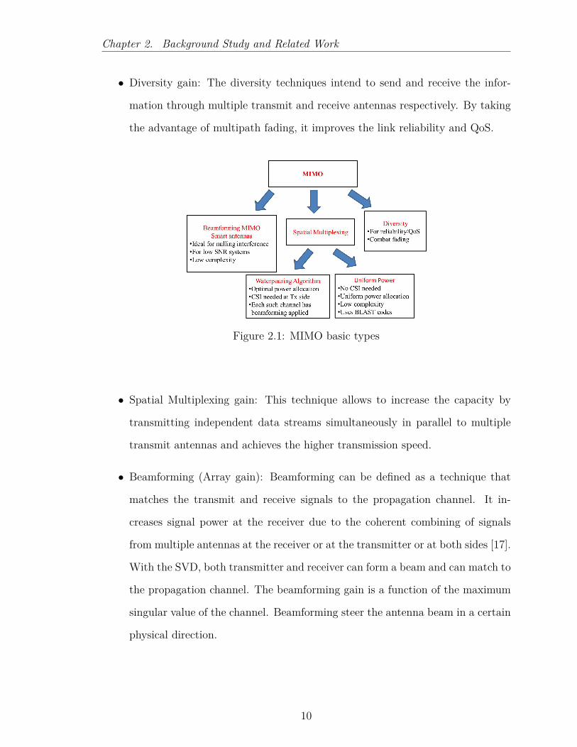
MIMO technology offers three gains: diversity gain, spatial multiplexing gain and
beamforming (array gain) [15] [16] as shown in Figure 2.1.
9
Chapter 2. Background Study and Related Work
• Diversity gain: The diversity techniques intend to send and receive the infor-
mation through multiple transmit and receive antennas respectively. By taking
the advantage of multipath fading, it improves the link reliability and QoS.
Figure 2.1: MIMO basic types
• Spatial Multiplexing gain: This technique allows to increase the capacity by
transmitting independent data streams simultaneously in parallel to multiple
transmit antennas and achieves the higher transmission speed.
• Beamforming (Array gain): Beamforming can be defined as a technique that
matches the transmit and receive signals to the propagation channel. It in-
creases signal power at the receiver due to the coherent combining of signals
from multiple antennas at the receiver or at the transmitter or at both sides [17].
With the SVD, both transmitter and receiver can form a beam and can match to
the propagation channel. The beamforming gain is a function of the maximum
singular value of the channel. Beamforming steer the antenna beam in a certain
physical direction.
10

Chapter 2. Background Study and Related Work
2.1.1 MIMO System Model
A single-user MIMO system consists of Mt transmit and Nr receive antennas as shown
in Figure 2.2. The channel can be represented with matrix H with Mt×Nr dimensions.
Figure 2.2: Mt ×Nr MIMO system.
The received signal vector y can be written as [18]:
y =√
ExMt
Hx + n (2.1)
where x = [x1, x2, ..., xMt ]T ∈ CM represents the complex-baseband transmitted sym-
bol vector and y = [y1, y2, ..., yNr ]T ∈ CN is the received vector related through an
Mt × Nr channel matrix H. A receiver noise vector n = [n1, n2, ..., nNr ]T ∈ CN is a
spatially white, zero-mean, circularly symmetric complex Gaussian noise vector, nor-
malized so that EnnH = INr . The total average energy of the transmitted signal is
denoted by Ex.
In a flat-fading channel, MIMO channel matrix H is represented by random complex
fading coefficients, where hij represents the channel gain from transmit antenna j to
the receive antenna i.
11

Chapter 2. Background Study and Related Work
2.1.2 MIMO Precoding
In MIMO systems, the output at the receiver is the mixture of multiple transmitted
signals. The main difficulty in MIMO channels is the separation of the data streams at
the receiver which are sent in parallel from the multiple transmit antennas. This prob-
lem can be solved by using a precoder with knowledge of the CSI at the transmitter
side, as shown in Figure 2.3.
Figure 2.3: A single-user MIMO system with linear precoding/decoding.
In time division duplex (TDD) systems, the uplink and downlink uses the same fre-
quencies and the transmitter can have channel knowledge through the reciprocity
principle. In frequency division duplex (FDD) systems, both links are not recipro-
cal and this information can be estimated at the receiver with channel estimation
techniques. This information needs to be sent back to the transmitter via low-rate
feedback channels.
If CSI is available at the transmitter, the transmitted symbols can be partially sepa-
rated by means of a precoder at the transmitter and can be received by using a decoder
at the receiver. With CSI at the transmitter side, the Singular Value Decomposition
(SVD) [19] model can be performed as shown in Figure 2.3. The transmitted signal is
pre-processed with V on the transmitter side and a received signal is post-processed
with UH on the receiver side.
12

Chapter 2. Background Study and Related Work
If SVD is performed on the matrix H, then it degenerates to:
H = UDVH (2.2)
where U and V are unitary matrices in (Nr × Nr)-dimension and in (Mt × Mt)-
dimension, respectively. Matrix VH is the conjugate transpose of the matrix V. It
is noticed that VHV = UHU = 1. The matrix D is a rectangular matrix, whose
diagonal elements are non-negative real numbers and off-diagonal elements are zero.
The diagonal entries of matrix D are the singular values of the channel matrix H,
σ1 > σ2 > ... > σrank, where rank = min(Mt, Nr). The squared singular values are
also known as the eigen-values of HHH : σi2(H) = λi(HHH). The SVD model decom-
poses the MIMO channel into independent parallel channels. The number of positive
singular values represent the possible number of independent sub-channels formed in
MIMO systems as shown in Figure 2.4. These independent channels λ1, λ2, ...λrank are
also known as eigenmodes [20] [21]. Thus, it is possible to send different streams of
data through the same number of independent channels as the number of eigenvalues
of H, this process is known as Spatial Multiplexing (SM).
The eigenvalues represent the gains of the individual links as shown in Figure 2.4. The
channel capacity can be improved if the transmission power is adaptively allocated
over the eigenmodes by using the WPA. Similarly, the data rate can also be optimized
by applying adaptive modulation schemes to the eigenmodes [22] [23]. In the adaptive
systems, the eigenvalues can be adjusted according to the propagation channel status
to boost the overall performance. This process requires precoder with CSI at the
transmitter and decoder at the receiver to decode the output signal.
13

Chapter 2. Background Study and Related Work
Figure 2.4: Eigenbeamforming transmission schematic.
2.2 MIMO Channel Capacity
The channel capacity of a communication system can be defined as the maximum
transmission rate for which a reliable communication is possible [17] in the system.
It is an important metric in closed-loop MIMO schemes that adapts the transmission
rate by adapting the channel quality information [24].
2.2.1 When CSI is Known to the Transmitter Side
When multiple antennas are present at both the link ends, the SVD decomposition,
gives the maximum number of data streams that can be transmitted simultaneously.
It can make the MIMO channel equivalent to virtual single-input single-output (SISO)
links and the MIMO channel capacity can be achieved by summation of all the SISO
links capacities.
By using SVD, the output signal at the receiver (2.1) as given in [18] [25] can be
14

Chapter 2. Background Study and Related Work
formulated as follows:
y =√
Ex
Mt
UHHVx + n (2.3)
By using (2.2),(2.3) can be written as:
y =√
Ex
Mt
Dx + n (2.4)
With SVD, the output is divided into r virtual SISO channels, the output across one
channel is,
yi =√
EsMt
√λixi + ni, i = 1, 2, ...., r. (2.5)
The transmit power for the ith transmit antenna can be written as γi = E|xi|2.
With the energy of the transmitted signal Ex and the power spectral density of the
noise N0, the capacity of the ith virtual SISO channel can be written as:
Ci(γi) = log2
(1 + Exγi
MtN0λi
), i = 1, 2, ...., r. (2.6)
The total available power at the transmitter is limited to the total number of transmit
antennas:
ExHx =Mt∑i=1
E|xi|2
= Mt (2.7)
As discussed earlier, with SVD, the channel capacity of MIMO is the sum of the
capacities of the virtual SISO links and can be written as:
C =r∑i=1
Ci(γi) = E
r∑i=1
log2
(1 + Exγi
MtN0λi
) (2.8)
The total power constraint as in (2.7) must be satisfied and the capacity can be
15
Chapter 2. Background Study and Related Work
maximized with the proper power allocation:
C = E
max∑r
i=1γi=Mt
r∑i=1
log2
(1 + Exγi
MtN0λi
) (2.9)
subject to ∑ri=1 γi = Mt. The optimization problem in (2.9) can be solved with some
threshold P as:
γopti =(P − MtN0
Exλi
)+
, i = 1, 2, ...., r.∑ri=1 γ
opti = Mt
(2.10)
where P is a constant and (z)+ is defined as:
(z)+ =
z if z ≥ 0
0 for z < 0(2.11)
The solution in (2.10) satisfying the constraint in (2.11) is the well-known WPA [2]
for power allocation in MIMO channels, that is shown in Figure 2.5. It indicates
that more power must be allocated to the eigenmodes with higher SNR denoted as
used modes. If the value of SNR is below the threshold level in terms of P, the
corresponding eigenmodes must not be used and no power is allocated to unused
modes.
2.2.2 When CSI is not Known to the Transmitter Side
When the channel matrix H is not known at the transmitter side, the optimal strategy
is to divide the total power equally across all the transmit antennas. The autocorre-
lation function of the transmit signal vector x can be represented as:
Rxx = IMt (2.12)
16

Chapter 2. Background Study and Related Work
Figure 2.5: Water-pouring power allocation algorithm.
Without CSI at the transmitter, the channel capacity can be written as:
C = E
r∑i=1
log2
(1 + Ex
MtN0λi
) (2.13)
where r represents the rank of H or the possible number of spatial links in the MIMO
channel, or rank(H) = min(Mt, Nr). In (2.13), the channel gain for the ith SISO
channel is λi. The total channel capacity in (2.13) is different from (2.8) without the
knowledge of CSI at the transmitter and the total power is allocated uniformly to all
transmit antennas.
2.3 MIMO Channel Quality Metrics
With the introduction of MIMO technology, a considerable amount of research has
been published on eigenvalue statistics [10] [26] to explore the channel quality metrics.
Knowledge of the eigenvalue statistics has shown the many advantages of MIMO in
terms of SM gain, diversity order and beamforming gain [27] [28].
17

Chapter 2. Background Study and Related Work
The eigenvalues of the correlation matrix reveal important characteristics in terms of
the spatial domain of MIMO channels. The eigenvalue spread (EVS) indicates the
spatial selectivity of the MIMO channels. It gives an indication about how many
spatial links are possible within the MIMO system. If the eigenvalue spread is high,
it shows the channel is more correlated with high difference between the eigenvalues.
With knowledge of the EVS, it is possible to inject power effectively into the channels.
In the high SNR regime, greater channel capacity can be achieved if the eigenvalues
are less spread out. In the low SNR regime, all the power can be allocated to the
strongest eigenmode to attain high beamforming gain.
Several studies have employed the eigenvalue-dependent channel quality metric as a
switching criterion in adaptive MIMO systems [29] as depicted in Figure 2.6. The
channel is estimated at the receiver end with the channel estimation techniques and
the channel quality metric is computed based on these estimates. The transmitter is
then informed with a low-rate feedback link.
Figure 2.6: Adaptive MIMO system.
Based on feedback information, the transmitter selects the appropriate signalling pa-
rameters like modulation and coding techniques for the next transmission. This makes
the system adaptive where the transmitter adapts to the changes of the propagation
18

Chapter 2. Background Study and Related Work
channel. Thus, the channel quality metric acts as a switching criterion for certain
adaptive MIMO systems [24] [30] to improve the link quality.
2.3.1 Rank
The MIMO channel capacity is highly dependent on the propagation channel char-
acteristics even if the CSI is perfectly known at the transmitter (CSIT) and at the
receiver side (CSIR). One of the important parameters of the MIMO channel ma-
trix is the rank, which reveals important MIMO system characteristics in the spatial
domain. It represents the effective spatial links that are possible within the MIMO
channel. The rank of the MIMO channel matrix indicates the number of data streams
that can be spatially multiplexed on a MIMO link.
A high rank of MIMO channel matrix indicates a radio channel with rich scattering,
which leads to several independent spatial channels. A low channel rank indicates
that spatial paths are highly correlated. With the channel rank one, only a principal
propagation direction is possible as in the case of beamforming. For adaptive trans-
mission, rank has been used as a channel metric to improve the detection performance
of the Bell Laboratories Layered Space-Time (BLAST) in spatially correlated MIMO
channels [31].
2.3.2 Condition Number
The condition number (CN) is another channel quality metric which reveals the mul-
tipath richness of the MIMO channel [32]. It measures the amount of correlation
present in the MIMO channel. A channel rank only provides the possible number of
spatial links but does not give any information about the quality of the links. A CN
indicates the channel quality and is related to the EVS of the channel matrix. The
19

Chapter 2. Background Study and Related Work
CN denoted as (κ) can be defined as the quotient of maximum eigenvalue and the
minimum eigenvalue of the channel matrix as:
κ = λmaxλmin
(2.14)
where the λmax and λmin represent the maximum eigenvalue and the minimum eigen-
value, respectively. A detailed knowledge of the eigenvalue spread is highly desirable
to characterize the MIMO propagation channel for future wireless communication
systems.
Most research work has used the CN as a selection criterion for several purposes in
MIMO systems. Heath and Love [30] used a CN of the MIMO channel to perform
multimode antenna selection with limited feedback. In another study [33], Heath
and Paulraj used CN of the MIMO channel to perform switching between diversity
and multiplexing gain purposes. In a similar way, Piazza et al. [34] used CN to
switch between different modes of circular patch reconfigurable antennas. For the
adaptive modulation scheme, CN was used by Forenza et al. [35] to obtain the spatial
selectivity of the channel. Previous work in [36], demonstrates the use of regular CN
(or its reciprocal) to evaluate the quality of the channel matrix as it provides some
intuition on channel quality.
Heath and Paulraj have proposed another switching criterion to choose between SM
and diversity schemes in [33], known as the Demmel condition number. It has been
shown that the Demmel condition number (κD) of the matrix channel provides a
sufficient condition for multiplexing to outperform diversity. The Demmel condition
number is the ratio of the Frobenius norm and the smallest singular value. A Demmel
condition denoted by κD can be written as:
κD =∑mi=1 σiσmin
(2.15)
20

Chapter 2. Background Study and Related Work
where λmin is the minimum singular value of the channel matrix. In [37], MIMO Or-
thogonal Frequency Division Multiplexing (OFDM) channel measurements have been
carried out to study the statistical properties of κD in various propagation environ-
ments.
A CN is a metric of the channel quality and also indicates the sensitivity of the MIMO
channel matrix. A value of CN close to one indicates a well-conditioned matrix with
almost equal eigenvalues. A high value of CN indicates a correlated channel with a
large difference between all the eigenvalues of the channel matrix. Thus, high CN also
signifies the rank drop and degenerates into a rank-1 channel matrix. Statistically,
if the channel condition number is low then the channel will be more suitable for
large capacity gains for SM in MIMO wireless systems [32]. The importance of the
condition number in the area of MIMO communications has been discussed by many
authors in [38–42].
The condition number also indicates the behaviour of the channel matrix H: as an ill-
conditioned channel matrix or a well-conditioned channel matrix. An ill-conditioned
channel matrix means that small changes at the input side can make drastic changes
in the solution channel matrix. During matrix computations, these small changes are
caused by round-off errors and the solution of the channel matrix becomes unreliable.
The ill-conditioning of the matrix also shows the singularity property of the matrix,
which thus becomes non-invertible. Moreover, this computational complexity also
makes the architecture design of the receiver more complicated [19].
If the CN of a matrix approaches 1, then that matrix is known as well-conditioned
matrix. In the high SNR regime, a well-conditioned MIMO channel matrix, can
facilitate communication with high SM gain. In the low SNR regime, allocating power
to the strongest eigenmodes and leaving the weak eigenmodes with no power allocation
is the best policy to attain beamforming gain. The achieved channel capacity in terms
21
Chapter 2. Background Study and Related Work
of eigenmodes can be written as [43]:
C ≈ P
N0
(maxiλi
)log2e, bits/s/Hz (2.16)
where maxiλi is the maximum power gain provided by the MIMO channel. In the
low SNR regime, the effect of the rank or CN of the MIMO channel matrix becomes
negligible.
2.4 MIMO Channel Modelling
When communicating over MIMO fading channels, it is necessary to consider the
system architecture and the particular propagation environment conditions. The dis-
tribution of the channel matrix H can be drawn from a certain probability function.
It characterizes the MIMO system with the propagation scenario of interest and is
known as the channel model. The modelling of MIMO channels captures the key prop-
erties of the propagation environment and evaluates the system performance. It is
also important in system analysis, network planning and design in terms of signalling
and detection schemes. It also enables the performance prediction and comparison of
different system configurations in various propagation environments.
2.4.1 MIMO Channel Models
Several channel models for MIMO systems have been proposed previously in the
literature [44–46], and can be classified in different ways. Two main categories of
MIMO channel models are: Propagation-based models and Analytical models.
• Propagation-based models: are also known as physical channel models. The
22

Chapter 2. Background Study and Related Work
physical channel model chooses physical parameters to describe the MIMO
propagation channels. These parameters include angle-of-departure (AoD) at
transmitter, angle-of-arrival (AoA) at receiver, antenna spacing at both ends
and path attenuation [7]. This channel model reproduces the physical wave
propagation in a deterministic or stochastic way.
The deterministic models aim to characterize the actual physical radio prop-
agation environment channel. The channel matrix can be generated based on
a geometrical description of the propagation environment by employing ray-
tracing techniques combined with knowledge of the propagation environment.
The mathematical derivation of these models is complex and time consuming.
Thus, they are used only to cover specific small indoor environments.
The stochastic models aim to consider the channel behavior as a random vari-
able with a certain statistical distribution depending on the propagation envi-
ronment. These models are often based on large measurement data. Empirical
models, which are based on channel measurements, also fall into this category.
• Analytical channel models focus on modelling the spatial structure of the chan-
nel without considering the characteristics of the propagation environment. Two
popular models which characterize the MIMO channel matrix in terms of the cor-
relation between the matrix coefficients are: independent identically distributed
(i.i.d.) Rayleigh fading, and Kronecker channel models [44].
This thesis focuses on MIMO channels which follows the Rayleigh fading channel
model. There are various models for the correlation structure on this fading. De-
pending on the structure, the correlation can be exploited on transmit/receive or on
both sides.
23
Chapter 2. Background Study and Related Work
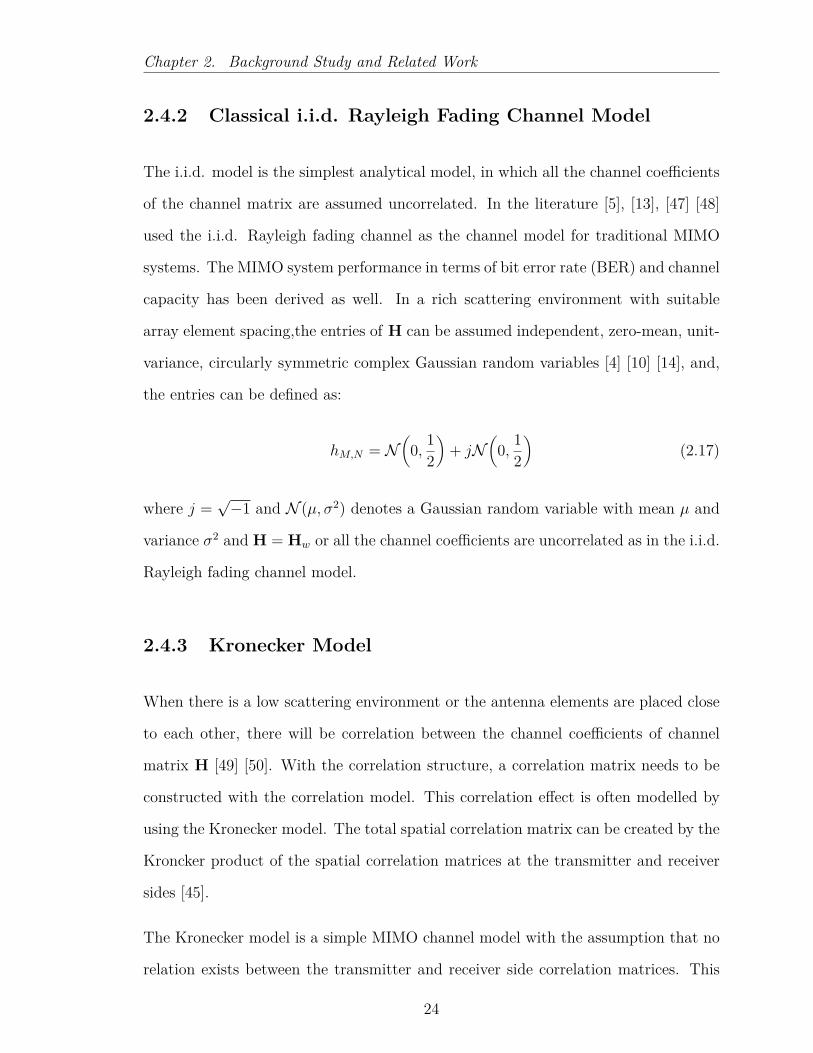
2.4.2 Classical i.i.d. Rayleigh Fading Channel Model
The i.i.d. model is the simplest analytical model, in which all the channel coefficients
of the channel matrix are assumed uncorrelated. In the literature [5], [13], [47] [48]
used the i.i.d. Rayleigh fading channel as the channel model for traditional MIMO
systems. The MIMO system performance in terms of bit error rate (BER) and channel
capacity has been derived as well. In a rich scattering environment with suitable
array element spacing,the entries of H can be assumed independent, zero-mean, unit-
variance, circularly symmetric complex Gaussian random variables [4] [10] [14], and,
the entries can be defined as:
hM,N = N(
0, 12
)+ jN
(0, 1
2
)(2.17)
where j =√−1 and N (µ, σ2) denotes a Gaussian random variable with mean µ and
variance σ2 and H = Hw or all the channel coefficients are uncorrelated as in the i.i.d.
Rayleigh fading channel model.
2.4.3 Kronecker Model
When there is a low scattering environment or the antenna elements are placed close
to each other, there will be correlation between the channel coefficients of channel
matrix H [49] [50]. With the correlation structure, a correlation matrix needs to be
constructed with the correlation model. This correlation effect is often modelled by
using the Kronecker model. The total spatial correlation matrix can be created by the
Kroncker product of the spatial correlation matrices at the transmitter and receiver
sides [45].
The Kronecker model is a simple MIMO channel model with the assumption that no
relation exists between the transmitter and receiver side correlation matrices. This
24

Chapter 2. Background Study and Related Work
means the correlation present at the receiver side is independent from the correla-
tion present at the transmitter side. Thus, each transmitter shows its own transmit
correlation matrix, regardless of the receiver, and each receiver shows its own receive
correlation matrix, regardless of the transmitter.
The Kronecker channel model approximates the correlation matrices by using trans-
mitter and receiver correlation matrices and can be written as [45] [51–53]:
H = R1/2R HwR1/2
T (2.18)
where RT and RR represents the correlation matrices at the transmitter and re-
ceiver sides, respectively. The channel matrix Hw is represented with i.i.d. zero-mean
complex-Gaussian entries.
2.5 Role of Channel State Information
In MIMO systems, knowledge of the channel state at the transmitter/receiver or on
both sides improves the system performance. The importance of channel knowledge
has been previously discussed [54], and results showed the loss of degree-of-freedom
(DoF) with the lack of availability of perfect CSIT. The performance in MIMO systems
is degraded with no channel information available at the transmitter side, even if the
receivers have CSIR. CSIT can be achieved either by exploiting the channel reciprocity
principle in a TDD system or by means of a limited feedback channel in FDD system.
25

Chapter 2. Background Study and Related Work
2.5.1 Channel Knowledge at the Transmitter
It is often assumed that the receiver can track the channel perfectly and thus complete
CSI is possible at the receiver side (CSIR). But the transmitter can have different levels
of CSIT, ranging from no CSIT at all to full CSIT. The assumption of accurate channel
information is possible at the receiver side especially in the downlink. It is possible
by using channel estimation techniques employing a common pilot-symbol channel
shared between both terminals. The transmitter relies on the channel measurements
at the receiver side and can be informed by the receiver in an implicit or explicit way.
Channel acquisition at the transmitter mainly relies on channel reciprocity or feed-
back. In FDD systems, where channel reciprocity cannot be exploited, the need for
CSIT places a significant burden on the bandwidth constraints of the feedback chan-
nels. These feedback requirements further worsen in high-mobility systems (such as
3GPP-LTE,WiMAX etc.) where the channel conditions change rapidly and in wide-
band systems with frequency selective channels that require more feedback bits.
2.5.2 Statistical Channel Knowledge at the Transmitter
Because of the feedback bandwith constraint (availability) in wireless communication
systems, it is not possible to send back all of the information from the receiver to
the transmitter. Another option is to send partial channel state knowledge with less
feedback overhead, also known as statistical CSIT. The reason for using statistical
feedback is that the second-order information of the channel statistics vary much
more slowly in comparison to the channel realization itself. This statistical CSIT
can be conveyed periodically to the BS resulting in little uplink overhead in terms of
feedback bits.
In the literature [44] [55], two common models for statistical CSIT that have been
26

Chapter 2. Background Study and Related Work
studied extensively are:
• Channel Mean Information (CMI): refers to the case where the channel at the
transmitter is assumed with a nonzero mean while the covariance matrix is
unknown and often assumed as white.
• Channel Covariance Information (CCI): refers to the case where the channel
at the transmitter is assumed with zero mean while the information regarding
the relative geometry of the propagation path is available through a non-white
spatial covariance matrix.
Channel knowledge acquisition at the transmitter side using covariance feedback can
be applied to both TDD and FDD systems.
2.6 Antenna Selection in MIMO Systems
The use of multiple antennas at both ends of a wireless link offers significant improve-
ments in terms of channel capacity and link reliability. The deployment of MIMO
systems with multiple antennas is the major limiting factor in wireless systems. In
fact, antenna elements are cheap but the RF chains connected to antennas increase
the complexity in terms of space, and hardware requirements. In general, RF chains
include amplifiers, mixers, up-and-down converters and analog-to-digital converters
(ADC) on both sides, increasing the cost and power consumption as well. As dis-
cussed in the last section, there is another constraint of bandwidth requirement for
the feedback link to send the CSI back to the transmitter. An effective solution to
overcome all these disadvantages is antenna selection, which reduces the cost and size
while providing as high a data rate as conventional MIMO systems [56] [57–59].
A typical MIMO system, as in Figure 2.7, shows an antenna selection scheme at the
27

Chapter 2. Background Study and Related Work
transmitter and receiver side. The system consists of Mt transmit and Nr receive
antennas, whereas a lower number of RF chains have been selected at the transmitter
side (LMt < Mt) and at the receiver side (LNr < Nr). The best sub-set of LMt
transmit and LNr receive antennas are selected with the antenna selection schemes.
In this way, it reduces the number of RF chains from Mt to LMt at the transmitter
side and from Nr to LNr at the receiver side, and therefore reduces the complexity of
the system. Thus, MIMO systems using AST employ a reduced number of RF chains
at the transmitter and receiver side.
Figure 2.7: Block diagram of MIMO system with antenna selection.
As shown in Figure 2.7, it is possible to select the subset of the best antennas at
the transmitter and receiver side. The feedback overhead can also be reduced by
using transmit antenna selection. The receiver can send back the CSI with a low-rate
feedback channel and select the antennas at the transmitter side. Thus, AS reduces
cost, space and complexity in terms of RF chains and feedback bits.
The antenna selection process, selects the subset of antennas that maximizes some
channel metrics in the system. The difference between antenna selection at the trans-
mitter and the receiver side is the usage of the feedback. The selection of the transmit
antennas can be selected at the receiver side and the information can be fed back to
the transmitter. As only indices of the transmit antennas need to fed back, it reduces
28

Chapter 2. Background Study and Related Work
the feedback overhead.
The optimal choice for antenna selection in MIMO systems requires knowledge and
estimation of the full channel matrix H. To estimate all the channel coefficients with
all the antennas, it seems necessary to make available all the RF chains on both sides.
But this goes against the goal of reducing the number of RF chains. In the antenna
selection process, when the environment changes slowly and with the help of a training
sequence, antennas can be multiplexed to different RF chains so that the channel is
estimated successively antenna by antenna.
Many algorithms for antenna selection have been investigated in the literature [60–62],
which can be classified as transmit antenna selection, receive antenna selection, or
joint transmit-receive antenna selection. The antenna selection criteria can be chosen
to optimize different performance metrics, such as maximizing theoretic capacity [63]
[64–66], maximizing SNR, or minimizing error rate [67] [68] [69] etc. These algorithms
can be applied at the either side of the link [70].
Some algorithms in the literature are related to the topic of this thesis, and can be
summarized as follows:
• Incremental antenna selection technique (IAST)
• Decremental antenna selection technique(DAST)
In IAST, each antenna is added successively at each step, the antenna that contributes
most to the increase of the channel capacity is added to the set of selected transmit
antennas. The antenna that provides the highest capacity is selected first, then the
antenna which provides second highest, and so on. This process continues until all
transmit antennas are selected [56].
Another antenna selection algorithm, DAST, can be implemented by deleting each
29

Chapter 2. Background Study and Related Work
antenna in descending order of decreasing channel capacity. It starts with all the avail-
able transmit antennas and selects the antenna that contributes least to the channel
capacity. One antenna in each step is discarded according to its capacity contribution.
Thus, DAST identifies and discards the antenna that yields the minimum contribution
to the capacity. The complexity of the DAST is higher than the IAST [25].
The straightforward approach for selecting the optimal subset of antennas is to ex-
haustively search over all the possibilities. The complexity of MIMO transceiver
algorithms increases exponentially with the number of transmit and/or receive an-
tennas. The selection of the subset antennas affects the channel capacity equation
in an iterative algorithm, which evaluates all possible antenna combinations to get
the highest channel capacity. In practice, fast and precise subset antenna selection
methods are required. However, the success of these selection algorithms depends on
the knowledge of CSI available at the transmitter and receiver side to select the best
subset of antennas respectively [71] [72] [73].
2.7 Antenna Array Design
Wireless communication system performance depends on the characteristics of the
propagation environment and the antenna array structure. Since the antenna interface
is also included in the communication channel between transmitter and the receiver,
the properties of the antennas also affects the signal quality of the system. Traditional
antennas integrated on devices such as laptops or on portable devices have fixed
radiation patterns. The properties of these radiation patterns do not change with
the changing environmental conditions. Thus, the performance of the communication
system degrades as the antennas do not operate optimally, according to the changing
conditions of the channel. To solve this antenna problem, reconfigurable antennas
30

Chapter 2. Background Study and Related Work
that can change their properties such as operating frequency, radiation pattern and
polarization, have gained significant interest. These antennas are considered smart
antennas and can maximize the capacity of wireless systems [74].
MIMO system performance is strongly influenced by the interaction between the prop-
agation channel and the antenna array arrangement. The arrangement of the antenna
arrays in MIMO is mostly affected by these three parameters: spatial correlation, mu-
tual coupling and diversity. Thus, these three parameters should be taken into account
when evaluating the performance of the MIMO array.
2.7.1 Correlation
MIMO channel capacity increases linearly with the minimum number of transmit and
receive antennas when the channel coefficients are i.i.d complex Gaussian random
variables. But putting too many antennas on a portable device leads to high spatial
correlation. The correlation between the output signals reduces the spectral efficiency
and degrades the system performance of the MIMO system. To gain the benefits of
MIMO systems, it is important to find the methods to control the correlation effect
in the antenna array design.
2.7.2 Mutual Coupling
Mutual coupling has a significant impact on the implementation of MIMO technology,
especially on the portable devices where inter-element distance between antenna ter-
minals is very low. When antennas are placed close to each other, the electromagnetic
interaction between the closely spaced antennas is known as mutual coupling. Due
to this interaction, the current on each antenna not only attains its own current from
the feeding point but also induced current from the neighboring elements [75].
31

Chapter 2. Background Study and Related Work
The mutual coupling between antenna elements depends on a number of factors,
including inter-element spacing, operating frequency of the antennas, antenna array
structure, antenna array geometry, the radiation patterns of the antenna elements and
near-field scatterers. Most of these parameters can be estimated except the near-field
scatterers. Moreover, these scatterers in the propagation environments are random in
nature and increase the mutual coupling between the antenna elements.
Due to the close proximity of the antenna terminals, there are electromagnetic inter-
actions between the antennas that alter the radiation properties of the array. These
radiation patterns are not independent in the case of a MIMO system where the mul-
tiple antenna elements are placed with small separation. The negative effect of the
mutual coupling is the impedance matching that reduces the received power and SNR.
Mutual coupling not only influences the antenna efficiency [76] but also affects the
correlation. In the literature [77], it has been is shown that mutual coupling shown
significantly reduces the correlation and thus increases the channel capacity. It has
also been shown that mutual coupling can have a negative effect where it increases
the correlation and decreases the channel capacity.
High mutual coupling creates pattern diversity, where the individual patterns may
change, and reduces the correlation between the signals at the receiver. High mutual
coupling between the radiation signals at the receiver increases the spatial correlation
and impacts on the MIMO channel capacity [78] [79]. Different radiation patterns
means each antenna element radiates through different propagation links with different
portions of the scatterers. This is very helpful in MIMO systems especially in the case
of poor scattering environments. Thus, mutual coupling shows different radiation
patterns even when the antenna elements are separated with small spacings. These
radiation patterns can be calculated and measured with the Sij parameters of the
scattering matrix.
32

Chapter 2. Background Study and Related Work
Many studies have investigated the effect of mutual coupling on the MIMO systems.
Research has shown [80–82] the benefits in terms of the MIMO diversity gain by re-
ducing the signal correlation for a specific range of antenna separations. Other stud-
ies [49] [83] showed that mutual coupling degrades the MIMO performance in terms
of channel capacity and impedance mismatch between antennas and their termination
loads.
2.7.3 Diversity
MIMO antenna arrays can be designed with diversity techniques to reduce the signal
correlation between the antenna elements and hence can improve the system perfor-
mance. To obtain uncorrelated signals, different antenna diversity techniques are as
follows:
• Spatial diversity: This is the simplest and most common form of diversity
technique used in MIMO systems. The antennas are placed far apart from each
other to produce the phase delay between the received signals at the antennas.
Thus, the signal received at the first antenna is uncorrelated from the signal
received at the second antenna. When the antenna terminals are placed far
apart, propagation multipath impinges different array elements with different
phases, producing uncorrelated signals across different antennas.
Uncorrelated signals at the receiver depend on the appropriate spacing between
the antennas and the width of the multiple angle of arrival depending on the
scattering environment. However, benefits of the space diversity can be achieved
by producing uncorrelated signals. So if one of the signal is in deep fade, the
output signal can be recovered from the other antenna terminal. In typical
MIMO systems, where size and cost are the primary constraints, for example
33

Chapter 2. Background Study and Related Work
in mobile phones, placing antennas far apart is not possible for future wireless
communication systems.
• Pattern diversity: produces uncorrerlated signals across different array ele-
ments with orthogonal radiation patterns. These different radiation patterns
provide a high gain in a large portion of angle space, known as angle diver-
sity. The antennas are located in the same physical space but the multipath
signals come from the different angles. All the antenna array elements have a
different radiation pattern that points in a different direction, and thus receives
uncorrelated signals.
Vaughan [84] discussed reconfigurable antennas with different radiation patterns
to exhibit pattern diversity. The beamforming antenna provides an example of
pattern diversity, as it can direct its radiation pattern in different directions.
The radiation beams departing and arriving in different directions are added
destructively or constructively resulting in different channels. The pattern di-
versity helps to achieve independent multipath signals at antenna elements.
• Polarization diversity: obtains uncorrelated signals across different antenna
array elements by using cross-polarized antennas [85]. These antennas receive
multipath signals with different polarizations of the electric and magnetic field.
Unlike spatial diversity, these antennas can be located at the same position but
receive orthogonal polarization signals. A polarization reconfigurable antenna
can be designed to switch between linear polarizations, clockwise or counter-
clockwise in circular polarizations and different axial ratios and tilt angles of
elliptical polarizations [74].
34

Chapter 2. Background Study and Related Work
2.8 Induced EMF method
The induced electro motive force (EMF) method is a classical method to calculate the
self and mutual impedances of the antenna array elements. This method is easy to
calculate, gives a good approximation which leads to closed-form solutions to provide
very good design data [86]. When antennas placed in the close proximity, the mutual
coupling effect can not be ignored. The mutual impedance between the antenna array
elements is used to measure these mutual coupling effects.To analyze mutual coupling
effect between closely spaced antenna elements, it is necessary to know the fields
produced by the antenna at near distances [87].
Consider two parallel linear dipoles as shown in Figure 2.8, to calculate self and mutual
impedances of the antennas placing close to each other [87]. The distance between
two-dipoles along the x-direction is d and their centers are offset by b along the z-axis
direction.
Figure 2.8: (a) Two parallel linear dipoles (b) Equivalent Two-port network.
When antenna element-1 acts as driven element and other antenna element-2 acts as
open-circuited, there will be open-circuit voltage (V21,OC) on antenna-2, due to the
35

Chapter 2. Background Study and Related Work
mutual coupling effect. The mutual impedance at antenna element-2 due to antenna
element-1 with input current I1 on antenna element-1 can be written as :
Z21 = V21,OC
I1(2.19)
With the reciprocity theorem, Z12 = Z21. In the presence of incident field Ein, the
short-circuit current can be defined as [87]:
ISC = 1V0
∫ h
−hEin(z)I(z)dz (2.20)
where h defines the length of the antenna. and open-circuit voltage can written as:
VOC = − 1I0
∫ h
−hEin(z)I(z)dz (2.21)
The z-component of the electric field generated by antenna element-1 and incident
on antenna element-2 can be represented by E21(z). If antenna element-2 is open-
circuited then according to (2.21), the induced open-circuit voltage can be written
as:
V21,OC = − 1I2
∫ h2
−h2E21(z)I2(z)dz (2.22)
where h2 = l2/2 and I2(z) = I2(0) is the current on antenna element-2.
Substitute (2.22) in (2.19), the mutual-impedance at antenna element-2 due to an-
tenna element-1 will be:
Z21 = − 1I1I2
∫ h2
−h2E21(z)I2(z)dz (2.23)
36
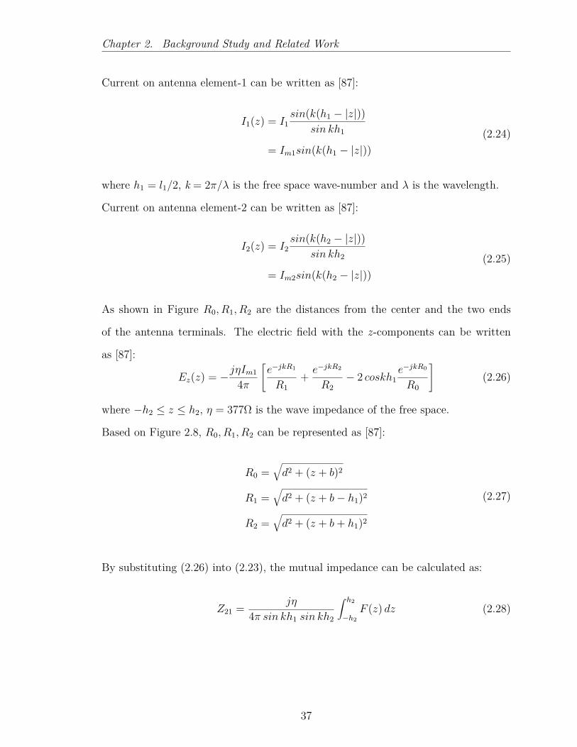
Chapter 2. Background Study and Related Work
Current on antenna element-1 can be written as [87]:
I1(z) = I1sin(k(h1 − |z|))
sin kh1
= Im1sin(k(h1 − |z|))(2.24)
where h1 = l1/2, k = 2π/λ is the free space wave-number and λ is the wavelength.
Current on antenna element-2 can be written as [87]:
I2(z) = I2sin(k(h2 − |z|))
sin kh2
= Im2sin(k(h2 − |z|))(2.25)
As shown in Figure R0, R1, R2 are the distances from the center and the two ends
of the antenna terminals. The electric field with the z-components can be written
as [87]:
Ez(z) = −jηIm1
4π
[e−jkR1
R1+ e−jkR2
R2− 2 coskh1
e−jkR0
R0
](2.26)
where −h2 ≤ z ≤ h2, η = 377Ω is the wave impedance of the free space.
Based on Figure 2.8, R0, R1, R2 can be represented as [87]:
R0 =√d2 + (z + b)2
R1 =√d2 + (z + b− h1)2
R2 =√d2 + (z + b+ h1)2
(2.27)
By substituting (2.26) into (2.23), the mutual impedance can be calculated as:
Z21 = jη
4π sin kh1 sin kh2
∫ h2
−h2F (z) dz (2.28)
37

Chapter 2. Background Study and Related Work
where F(z) is:
F (z) =[e−jkR1
R1+ e−jkR2
R2− 2 cos kh1
e−jkR0
R0
]sin (k(h2 − |z|)) (2.29)
Equation (2.23) referred as the mutual impedance across the input terminals of the
antennas. By normalizes (2.23), by the factor Im1Im2, the mutual impedance in (2.23)
can be represented as:
Z21m = jη
4π
∫ h2
−h2F (z) dz (2.30)
The self-impedance can also be calculated with (2.28) by setting h2 = h1 and d = a,
where a is the radius of the antenna element.
Thus, self-impedance can be written as :
Z11 = − 1I1
∫ h1
−h1E11(z)I1(z)dz
= jη
4π sin2 kh1
∫ h1
−h1F (z) dz
(2.31)
where F(z) is:
F (z) =[e−jkR1
R1+ e−jkR2
R2− 2 cos kh1
e−jkR0
R0
]sin (k(h2 − |z|)) (2.32)
By substituting d = a and b = 0 in (2.27):
R0 =√a2 + (z)2
R1 =√a2 + (z − h1)2
R2 =√a2 + (z + h1)2
(2.33)
The values of mutual impedance between the antenna elements and self-impedance of
38

Chapter 2. Background Study and Related Work
an antenna can be calculated by using (2.28) and (2.31) and respectively.
2.9 Reconfigurable MIMO Systems
Employing multiple antennas at both ends of the MIMO system provides diversity
and spatial multiplexing gain. The advantage of using such techniques increases the
reliability and spectral efficiency by taking the advantage of multipath propagation.
MIMO systems can adapt to varying channel conditions by adjusting the modulation
and coding rate and transmission signalling schemes according to the user’s need.
Placing multiple antennas at the transmitter and the receiver ends within a confined
space, especially on mobile terminals, puts a burden on the communication system.
Reconfigurable antennas are a promising solution to this problem. Reconfigurable
antennas act as smart antennas in which the system uses an antenna array and the
radiation pattern is dynamically adjusted by the system as required. Smart antenna
systems exploit their intelligence in order to generate or receive the desired radiation
pattern based on the RF environment. They have the ability to modify the an-
tenna characteristics by changing its frequency of operation, pattern and polarization
characteristics. Thus, reconfigurable antennas add an additional DoF in the MIMO
systems and can improve the overall system performance.
2.9.1 Techniques for Pattern Reconfigurable Antennas
Reconfigurable antennas have been studied over a decade for a variety of applications.
These antennas need various switching mechanism to achieve antenna reconfiguration
and optimal performance. There are different mechanisms in order to reconfigure the
antenna characteristics [74] [88]:
39

Chapter 2. Background Study and Related Work
2.9.1.1 Mechanical and Structural Changes
The antenna reconfiguration is achieved by modification of the mechanical changes by
using motors, actuators or other tools to move some parts in the antenna structure.
The change in the physical structure makes changes in the electrical properties of the
antennas and alters the radiation patterns. A mechanically movable mesh reflector
is used for a reflector antenna to achieve pattern reconfiguration as demonstrated
in [85]. The physical shape of a sub-reflector made of flexible conductor material can
be changed dynamically [89] to change the radiation patterns.
2.9.1.2 Electrical changes
Antenna reconfigurability can be achieved by using electronic switches to redistribute
the antenna surface currents. The electronic switches can connect and disconnect to
the antenna parts to redistribute the antenna currents. The integration of switches
to the antenna structures makes it possible to get the required pattern reconfigura-
bility. Electronics components such as positive intrinsic negative PIN diodes, micro-
electromechanical systems (MEMS) switches, optoelectronic switches and varactor
diodes can be used to redirect the surface current of antennas.
Different examples of electrically reconfigurable antennas are described below:
• PIN diode: The PIN diode is a semiconductor device, in which resistance
varies in accordance with the voltage applied through the anode and cathode
nodes. It operates in two states: in the on state, where the diode is forward
biased and this electronic component acts as short circuit and in the off state,
where the diode is reverse biased and this electronic component acts as open
circuit. It is a low-cost component with switching speed in the range of 1-100
ns [74]. In communication devices, it can handle power up to 40 dB.
40

Chapter 2. Background Study and Related Work
PIN diodes have been used in many antennas such as printed dipoles, slot anten-
nas, microstrip patch antennas, planar inverted-F antennas (PIFA), and dielec-
tric resonator antennas [90] owing to their high dynamic reconfigurable ability.
They have some drawbacks in terms of nonlinearity and DC power consumption.
• MEMS switch: MEMS switches rely on mechanical movement to achieve re-
configuration. These switches have advantages over PIN diodes such as: lower
insertion loss, higher isolation, minimum DC power consumption, and relatively
high power handling. They have very low switching speed in the range of 1-200
µs [74].
• Varactor diode:
The variation of the voltage levels in a varactor results in a change in its capac-
itance. Thus, they can tune the antenna operation in different regions. As com-
pared to PIN diodes, varactor diodes allow a tunable response. The advantage
of this type of component is its low DC consumption with efficient reconfigurable
ability [74] and it can be used in some adaptive wireless applications.
• Optoelectronic switch: Optical reconfiguration techniques based on the pho-
toconductive switches. The optoelectronic switch can reconfigure the patterns
in an antenna structure by using optical bias. An optical switch is formed when
a laser beam is incident on the semiconductor material. The shining light of op-
tical beam changes the activation and deactivation level of the photoelectronic
switch. It does not produce any harmonics and inter-modulation distortion due
to their linear behavior. Optoelectronic switches have some advantages such as
low losses, being lightweight, noise immunity, and RF-circuit isolation. Despite
all the advantages, optical switches have some issues in terms of integration with
antenna structures and require a complex activation mechanism [74].
41

Chapter 2. Background Study and Related Work
2.9.1.3 Material changes
Reconfigurable properties can also be attained through material changes. Change in
material characteristics alter the current distribution of the antenna element resulting
in steering the radiation pattern in different directions. The changes in the material
characteristics contribute to shift the antenna frequency and changing the permittivity
of the material alters the antenna length.
Antenna substrate characteristics can be changed by using materials like liquid crys-
tals and ferrites. The changes in these materials can be obtained by changing the
relative magnetic permeability or electric permittivity. In a liquid crystal material,
the orientation of the liquid crystal molecules can be altered. By doing this, the
dielectric constant can be changed with different voltage levels. For ferrite materi-
als, permittivity and permeability can be changed with applied electric and magnetic
fields respectively [88].
In non-resonant antennas, the beam steering capabilities can be changed with the
propagation speed of the traveling waves. Two-dimensional grid array of resonant
slot antennas can be built on a conventional substrate using ferrostrate material. By
changing the permittivity of the ferroelectric superstrate, beam steering capability can
be attained [91]. Other antenna designs have been investigated [92] that used this
technique to steer the beampatterns. Slab in [93] also studied leaky wave antennas
that rely on material changes to steer the beam in different directions. This has
some drawbacks such as slow tuning speed, small reconfiguration capabilities and
high voltage requirements.
42

Chapter 2. Background Study and Related Work
2.9.2 Types of Pattern Reconfigurable Antennas
In pattern reconfigurable antennas, a single or a small number of active elements is
surrounded by a ring of parasitic elements loaded at their base with some load in
the form of a reactance or switch. The antenna elements connected to the RF source
are referred to as active or driven elements. The parasitic elements are not active
because they are not connected to any RF source. They are placed in close-proximity
to the active elements. The loads can be electrically controlled to form and steer
the radiation pattern of the array. The signals are coherently combined before being
detected by the elements, and therefore they do not suffer from quantization errors in
individual elements. The radiation pattern control is achieved by adjusting the phases
of currents in the passive radiators via electronically controlling the impedance loads
connected to the parasitic elements. Antenna symmetry allows these beams to be re-
peated through the azimuth plane with appropriate stepping of loading configurations
around the parasitic ring.
There are two general categories of pattern reconfigurable antenna systems, namely
the adaptive array and switched array as discussed below [94] [95]:
2.9.2.1 Adaptive array system
An adaptive array system is a smart antenna system configuration with an infinite
number of patterns based on the propagation scenario. In adaptive array design,
radiation patterns alter dynamically in response to the changing RF environment.
With the use of signal processing algorithms, adaptive systems are able to distinguish
between the desired signal and the interference signal. In a fully adaptive array, the
beam patterns can be pointed into arbitrary directions. This allows direction the
main beam to the desired user and at the same time nullifies the interference. By
43

Chapter 2. Background Study and Related Work
doing this, the signal-to noise and interference ratio (SINR) can be maximized.
Based on N-port scatterer theory, Harrington proposed, a seven-element dipole array,
in which one active radiator is surrounded by six equivalent parasitic elements. These
parasitic elements are loaded at their center with a variable reactance. These reac-
tances are typically produced with varactor diodes. The depletion level of the diode
can be controlled with reverse bias magnitude. The variable reactances afford fine
analog control of radiation. The variable loads alter the values of the reactance and
steer the beam in different directions.With appropriate algorithms, the antenna can
be termed as adaptive due to the load’s ability to form a main lobe in one direction
and nulling others. The control circuitry for the varactor requires a digital to analog
converter for analog reverse bias, and RF chokes to isolate the DC path from the
element. This control circuitry is simple to manufacture and relatively inexpensive
compared to the active phased array.
Harrington in [96] presented numerous load configurations to illustrate the antenna’s
beam steerability. This work is further investigated for path and monopole antennas
by Thiel and Smith [94], Thiel et al. [97], Sibille et al. [98], Preston and Thiel [99]
and Vaughan [100].
2.9.2.2 Switched array system
The switched array system is a smart antenna system configuration with an finite
number of patterns. These multiple fixed patterns are formed with different sensitivity
levels in the predefined directions. The switched array concept originates from the
Yagi-Uda dipole array [101]. The Yagi-Uda linear array comprises a reflective dipole,
single active dipole and numerous director dipoles to achieve highly focused radiation
[94] [87]. The reflector dipoles constitutes the backbone of a switched parasitic array.
44
Chapter 2. Background Study and Related Work
Gueguen in [102] describes a switchable antenna where several Yagi-Uda dipole arrays
share an active element. A diode is at the center of each reflector and acts as in
resonance when short circuited, allowing radiation scattering. On the other hand,
an open diode leaves the dipole out of resonance and lets radiation pass. This work
has been investigated for wire and patch structures by Thiel and Smith [94], Thiel et
al. [97], Sibille et al. [98], Preston and Thiel [99] and Vaughan [100].
A switched parasitic array consists of one active (driven) element connected to the RF
source of the transceiver. There are a number of parasitic elements terminated with
resistive loads surrounding the active element. When the parasitic element is loaded
with an inductive load, it acts as director. Then the parasitic element radiated away
from the driven element. When the parasitic element is loaded with an capacitive
load, it acts as a reflector. Then the parasitic element radiates toward the driven
element.
Both adaptive array and switched array systems attempt to increase the gain accord-
ing to the location of the user. The adaptive system provides optimal gain while
simultaneously identifying, tracking, and minimizing interfering signals. But the im-
plementation cost of adaptive array systems in terms of complexity and hardware
effort is more than the switched beam array.
2.10 Related Work
Work in the literature related to the topic of this thesis can be summarized as follows:
45
Chapter 2. Background Study and Related Work
2.10.1 Related Work on Switched Parasitic Antennas
• Migliore et al. [7] proposed an adaptive MIMO system employing parasitic ele-
ments to improve the channel capacity. The antenna array design consists of a
set of active antennas coupled to a set of parasitic elements that are terminated
with complex loads. They discussed adaptive MIMO numerically and experi-
mentally to show the performance improvement with less complexity and cost.
In the classical MIMO approach, antennas need a rich-scattering environment
to achieve the best performance. On the other hand, in adaptive MIMO due
to its adaptivity, it is able to achieve satisfactory performance even in a poor
scattering environment. The results of adaptive MIMO have also been com-
pared with the antenna selection technique. The behavior of parasitic elements
in adaptive MIMO described is in three different ways:
i. Firstly, the parasitic elements are able to exploit the electromagnetic field
in a much wider space as compared to the conventional MIMO. With para-
sitic elements, the adaptive MIMO system has the capability to collect the
information smartly not only on the active elements but also collects the
information on the parasitic elements. It, provides the freedom of collecting
more information by properly varying the parasitic loads.
ii. Secondly, the parasitic elements act as local scatterers around the active
elements. By changing the configurations of the terminated loads, the
parasitic elements acts in and out of resonance. Thus, they modify the
propagation scattering environment.
iii. Finally with parasitic elements, the MIMO antenna array can form dif-
ferent working states compared to the conventional MIMO with a fixed
channel state with all active elements only. By selecting one of the radia-
tion pattern configuration states, the overall radiation pattern of the array
46

Chapter 2. Background Study and Related Work
can be modified. Moreover, the adaptive MIMO antenna array can adapt
to the propagation environment.
An evolutionary algorithm has been used for experimental results and achieved
the maximum channel capacity in less than 10 iterations. Channel estimation
has not been discussed, since each new configuration with changing parasitic
elements results in a different channel realization. It has not been described how
this information can be fed back to transmitter with limited feedback overhead.
• Wennstrom and Svantesson [103] introduced an antenna design with SPA to
steer the radiation patterns electronically in MIMO systems. The design consists
of one active element that is connected to the transceiver and several parasitic
elements terminated with switchable loads. The parasitic elements switched be-
tween in and out of resonance in the same manner as the Yagi-Uda antennas,
to form diverse radiation patterns. By changing the controllable loads termi-
nated on parasitic elements, the current distribution on the parasitic elements
also changed on the elements of the array, altering the radiation patterns. They
introduced the oversampling approach that samples the electromagnetic field at
various angular directions within a symbol period.
In their work, parasitic elements are designed as monopoles on a ground plane
to achieve omni-directional properties. The SPA configuration proposed in this
paper was designed with 5-element and 7-element monopole wires to form 4-
direction and 3-direction symmetric antennas, respectively. In the 7-element
monopole SPA, an additional circle of parasitic elements were hardwired to
ground to increase the directivity.
The authors adopted the Space Time Block Code (STBC) concept [104] to ex-
ploit the correlation effects to evaluate the channel capacity in MIMO systems.
It was shown that the channel capacity obtained with the SPA was approxi-
47

Chapter 2. Background Study and Related Work
mately the same as the capacity obtained by conventional MIMO antenna ar-
rays.
The authors exploit the characteristics of SPA that offer several fixed beams but
in a small size for utilisation on mobile terminals.They showed that diversity is
possible by quickly switching the parasitic loads at the receiver with an oversam-
pling approach. But they have not discussed about the bandwidth expansion
and the increased adjacent channel interference.
• Bains and Muller [105] proposed a low-complexity receiver architecture using
parasitic elements for implementing a rotating antenna for MIMO receivers.
The parasitic elements give the possibility of creating a directive antenna beam
that is rotated 360 degree within the duration of a symbol period. By doing
this, spatial multiplexing is converted into frequency multiplexing and different
sub-channels are created in the frequency domain.
Instead of sampling the electromagnetic field with antennas at discrete spatial
points, they proposed oversampling of the electromagnetic field by using the
rotating receive antenna to maximize the channel capacity. Using a rotating
receive antenna maximizes the link capacity, but sampling at a rate higher
than the symbol rate causes a bandwidth expansion issue. At the receiver end
the bandwidth expansion makes it sensitive to adjacent channel interference.
Channel-statistics have not been discussed that can impact the MIMO channel
capacity. The authors have not mentioned the channel quality parameter which
can be sent back to the transmitter.
• Vaughan [100] presented SPAs through antenna pattern diversity. These low-
cost antennas provide diversity gain in hand-held terminals. The antenna design
gives an efficient radiation pattern to reduce the bit errors of the received sig-
nals. The basic principle was explained for examples of wire antennas. The per-
48
Chapter 2. Background Study and Related Work
formance of four wire antenna configurations was evaluated through computer
simulation using the method-of-moments (MoM) process. The four different
configurations are described as follows:
i. A wire antenna configuration with the two radiation patterns forming a
compact antenna. The experiment set up includes one active element sur-
rounded with three parasitic elements. One of the parasitic elements is
short-circuited and the other two are terminated with switchable loads.
ii. A wire antenna configuration with two radiation patterns in the half space.
The experimental set up is same as the first wire antenna configuration but
the short-circuited parasitic element is replaced by a ground plane.
iii. A wire antenna configuration the same as the multiple elements of a Yagi-
Uda antenna. In this, one active element is surrounded with multiple
parasitic elements separated with 0.2λ distance. The parasitic elements are
switchable and change their states from short-circuited to open-circuited.
iv. A wire antenna configuration with a lower directivity beam with fine ro-
tational control using 16-parasitic elements with a separation distance of
0.25λ. By switching the parasitic elements, adjacent patterns can be ob-
tained with the angle of 360/15=22.5. Thus, a large number of decorre-
lated patterns can be obtained through 16-parasitic element configurations.
• Sohn and Gwak [106] proposed a single-RF MIMO-OFDM system with a Beam
Switching Antenna (BSA) at the receiver side. The single-RF MIMO-OFDM
used a single front-end and steered the beam patterns in predefined directions.
The oversampling effect at the receiver side induces replicas in the frequency
domain. These replicas interfere with the desired signals at the receiver side and
degrade the system performance. The authors investigated this problem in a
more realistic environment with the OFDM system with co-existing systems in
49

Chapter 2. Background Study and Related Work
the neighboring frequency bands. Beam-steering is done with PIN diodes for fast
switching speed. Different replica interference avoidance (RINA) strategies are
proposed for co-existing and co-operating network situations. They presented
two important findings to avoid adjacent channel interference:
i. replica interference without co-existing systems can be reduced with proper
switching rate at the BSA receiver. The beam pattern switching rate at
the receiver should be an integer multiple of the product of the orthogonal
frequency division multiplexing (OFDM) sampling rate and the number of
receiving beam patterns.
ii. replica interference with co-existing systems cannot be avoided completely.
The replica interference depends on the status of the coexisting user and
beam switching capability of the user.
For the simulation results and analysis, three different RINA approaches are
suggested: maximum-capability RINA (MAX-RINA), Static RINA (S-RINA),
and Dynamic RINA (D-RINA). In addition to that, the overall network opera-
tion principles of the replica interference avoidance strategies are also presented
in the different scenarios.
• Piazza et al. [34] demonstrates a technique for antenna configuration selection
for reconfigurable circular patch antennas. They investigated the benefits of
MIMO reconfigurable antennas through a combination of adaptive antenna ar-
ray structure and adaptive algorithm to select the optimal pattern configuration
at the receiver. Three different novel classes of electrically multi element recon-
figurable antennas have been proposed in their work:
i. a reconfigurable printed dipole array that exploits the inter-element mutual
coupling between closely spaces dipoles to exploit pattern reconfigurability,
50

Chapter 2. Background Study and Related Work
ii. circular patch antennas capable of exciting higher order modes to exploit
pattern and polarization reconfigurability, and
iii. a two-port meta-material leaky wave array that can be reconfigured in
number of array configurations to achieve pattern reconfigurability.
The antenna configuration selection algorithm includes knowledge of the second-
order statistics and average SNR. The performance of the proposed algorithm is
also compared to the conventional MIMO system that estimates each antenna
configuration and then selects the optimal configuration. With the selection
algorithm, there is only need to estimate the channel for a single antenna con-
figuration independently of the number of array configurations. The training
sequence is allocated to only a single antenna to estimate the channel instead
of estimating all the array pattern configurations. This improved channel esti-
mation shows better SNR level at the receiver.
Authors showed the functionality of the selection algorithm depends on the dif-
ferences existing between the antenna array configurations. Their work focused
on the switching between the circular patch modes.
• Forenza et al. [35] proposed a reduced-complexity adaptive MIMO transmis-
sion technique for exploiting the capacity of spatially correlated channels. The
adaptive switching algorithm designed to switch between different transmission
schemes depending on the changing channel statistics. The switching criteria
is based on the statistical knowledge of the channel rather than the instanta-
neous CSI. The algorithm used spatial correlation and average SNR information
to select the link-quality region for a given transmission mode. The switching
algorithm showed substantial capacity improvement in various propagation en-
vironment scenarios. The simulation results revealed significant improvement
in system performance in terms of capacity and error-rate over non-adaptive
51

Chapter 2. Background Study and Related Work
systems.
• Yoshida et al. [107] presented a compact transceiver structure to enable the
mobile terminals to be miniaturized with a single front-end. The parasitic ele-
ments provides adaptive analog beam-forming, and switching between parasitic
elements provides the spatial multiplexing. In the single RF front-end MIMO,
the parasitic antenna elements are terminated with variable reactances. By con-
trolling the parasitic elements interdependently, orthogonal directivity patterns
are generated and receive spatially diverse signals.
This paper considers both advantages of adaptive beam-forming and spatial
multiplexing for compensating the switch penalty. The proposed architecture
requires the antenna switching frequency to be higher than the signal band-
width. Furthermore, statistical analysis of the antenna switching system with
parasitic elements is discussed theoretically. The simulation results confirmed
that the performance does not degrade with the increase of spatial correlation.
The results are also compared with the conventional MIMO in a high spatial
correlation environment. The computer simulation results are same as that of
the conventional MIMO with a distance of λ/8 between the elements.
• Jo et al. [108] achieved full spatial multiplexing gain with single radio in their
research. The SNR is measured at the receiver with a beam switching antenna
to obtain spatial multiplexing gain in an indoor MIMO environment. The tran-
sient time of the switches is reduced by using a fast-response switching device.
To achieve beam-steering at the transmitter and receiver, a single active element
is surrounded with two parasitic elements. The values of the reactive loads ter-
minated on the parasitic elements are pre-defined. Four different case scenarios
have been discussed for the analysis and experiment results. These results re-
vealed SM gain with a Long-Term Evolution (LTE) FDD downlink signal. The
52

Chapter 2. Background Study and Related Work
performance of the beam switching antenna is improved by 10 dB by reducing
the switching rate.
Jo et al. [109] recreated the experimental results by employing 4 × 4 MIMO
signals by using a beam-switching technique at the receiver side. Demodulating
the MIMO signal with a single-RF shows some degrading factors in terms of
bandwidth expansion and SNR reduction.
2.10.2 Related Work on MIMO Channel Capacity with AS
and CSI
Work in the literature that is related to the MIMO channel capacity in this thesis is
summarized as follows:
• Cuan-Cortes et al. [18] showed MIMO channel capacity improvements by em-
ploying antenna selection and power allocation algorithms. IAST selects the
antennas in increasing order of their contribution to the channel capacity. Then
an optimal power allocation algorithm allocates the transmit power to those
antennas accordingly. They discussed the influence of the correlation matrix on
the channel capacity. The effect of the covariance matrix is shown in correlated
and uncorrelated propagation environments. A comparison was presented be-
tween the traditional MIMO that allocates power uniformly to all the transmit
antennas and WPA that allocates more power to the antennas that contribute
more to the channel capacity.
The antennas are selected first with IAST and then the covariance matrix is
improved by allocating the transmit power to the antennas with WPA. The
results showed the optimal covariance matrix improves the channel capacity
significantly with proper selection of antennas and power distribution among all
53

Chapter 2. Background Study and Related Work
the transmit antennas. A comparison of results reveals that the channel capacity
has been improved with the modified covariance matrix. It has been presented
that the channel capacity shows upper bounds with the improved covariance
matrix.
54

Chapter 3
Switched Parasitic Antennas
This chapter gives a brief introduction of parasitic arrays and their fundamental mech-
anism of operation. The concept of N-port network theory is reviewed with the an-
tenna modelling concept in MIMO systems. Electromagnetic mutual coupling is the
basic concept that defines the directive nature of the parasitic array. The switch-
ing parasitic array structure is described with structural parameters and controllable
loading configurations. Based on the switching state of the parasitic elements, the
impedance matrix is calculated and different radiation patterns are attained. In the
simulation scenario, different testing platforms are studied to generate a number of
pattern configurations with switched parasitic antennas.
3.1 Basics of Parasitic Arrays
Smart antenna systems have the ability to adapt according to the system require-
ments. They can adjust transmit and receive radiation patterns of the antennas based
on the propagation environment. The use of parasitic elements in the smart antenna
reconfigures the radiation patterns in order to improve the system performance. Par-
55

Chapter 3. Switched Parasitic Antennas
asitic antennas have been widely used in military and commercial purposes.
The Yagi-Uda [101] antenna is the classical example of using parasitic element for
analog TV reception signal. As discussed in [87], the antenna array consists of one
driven element with several parasitic elements in a linear array. The driven (active)
element is connected to the RF port and has a resonant length. Multiple parasitic
elements control the radiation pattern by changing the mutual coupling between the
antenna elements. When the length of the parasitic element is slightly longer than
the driven element it acts as a reflector. Therefore it radiates the beam towards the
driven element. When the length of the parasitic element is slightly shorter than the
driven element it acts as a director. It then radiates the beam away from the driven
element. The length of the parasitic elements is mechanically fixed in the Yagi-Uda
antenna structure.
In this thesis, MIMO-SPA follows the same mechanism of Yagi-Uda with few active
elements connected to the transceiver and several parasitic elements arranged in a
circular array fashion. As opposed to the Yagi-Uda antenna, the length of the parasitic
elements can be varied by using terminated loads on the parasitic elements. The
resonant length of the parasitic elements can be switched between different levels.
Depending on the switching position, parasitic elements act as reflector and director
states. Thus, loading the parasitic elements by electronic means enables the radiation
patterns to be steered in different directions. This process is also known as electronic
beam-steering.
The beam steering capability can be achieved through the use of optimal impedance
load values that can be controlled adaptively or manually. Parasitic arrays loaded
with adaptively tunable loads are known as ESPAR. Alternatively, the parasitic array
loaded with switchable impedance loads are known as switchable parasitic antennas.
In both techniques, optimal combination of load values steer the beam patterns in dif-
56

Chapter 3. Switched Parasitic Antennas
ferent directions. The difference between these two techniques is the type of circuitry
used. The tunable loads in ESPAR antennas are usually reactive (inductive/capaci-
tive) in nature, whereas in SPA the switchable loads are usually resistive in nature.
The switching between the load values tunes the parasitic elements in and out of
resonance and toggles the parasitic elements between reflector and director states re-
spectively. The symmetry property of antenna arrays also plays a significant role in
the design and optimization process. Some of the radiation patterns show similar pat-
tern configurations owing to the symmetry property of the antennas. The symmetry
property occurs in antenna arrays with an even number of parasitic elements. The
number of radiation patterns depends on the number of parasitic elements and the
load combinations terminated on the parasitic elements.
Most of the literature [110] [111] [112] has presented ESPAR and SPA antenna ge-
ometries, where the active element is placed in the center and parasitic elements
are placed in a circle equidistant from the origin. By doing this, beam-steering can
be achieved only in the azimuth plane. With more than one ring of parasitic ele-
ments the beam-steering can be achieved in both planes i.e. elevation and azimuth
planes. In 1978, Harrington [96] introduced parasitic elements terminated with tun-
able impedance loads to obtain the radiation patterns. Later, Milne [113] replaced
these tunable loads with switchable loads to direct the beam patterns in different
directions.
3.1.1 ESPAR
The electronically steerable parasitic array radiator (ESPAR) is a smart antenna that
reconfigures the radiation patterns electronically by changing the load values. The
structure of these antennas consists of one active element situated at the center and
surrounded with a number of parasitic elements. The active element is connected
57

Chapter 3. Switched Parasitic Antennas
to the RF port and the parasitic elements are terminated with the reactance loads.
These reactance loads can be realized with varactor diodes [112] and the beam steering
can be achieved by tuning these varactor diodes. A DC voltage supply is required
for these varactor diodes. The capacitance value of these diodes can be changed by
varying the voltage levels. This changes the distribution of currents on the antenna
elements and tunes the radiation patterns of the ESPAR antennas [74].
In 2000, the ATR labs in Japan introduced an ESPAR antenna [110] [111] with (K+1)
elements as shown in Figure 3.1. The active element is placed in the middle and
connected to the transceiver. There is only one active element connected to the RF
port and it requires only one RF chain. Six parasitic elements (K=6) are placed
around the periphery of the active element. The parasitic elements are terminated
with varactor diodes.
Figure 3.1: Structure example of (K+1)-element ESPAR.
58
Chapter 3. Switched Parasitic Antennas
By controlling the values of the varactor diodes, the mutual coupling varies between
the active and parasitic elements. The configuration of the parasitic elements can be
switched between director and reflector states. Thus, the radiation patterns can be
exploited in different directions.
ESPAR antennas achieve high DoF for fully adaptive arrays with reactively controlled
parasitic elements. They also provide high beam steering resolution but introduce
delays during re-radiation in adaptive applications. These antenna designs require
more hardware components to control the varactor diodes. Several DAC circuits are
required to convert the digital microcontroller output to an analog voltage level.
3.1.2 Switched Parasitic Antennas
Switched parasitic antennas (SPA) are another option for reconfigurable antennas to
provide a pre-defined fixed number of radiation patterns. As compared to ESPAR,
SPA antennas are terminated with electronically switchable loads. The parasitic el-
ements can be switched between reflector and director states through the use of RF
switches. These switches can be toggled between two states which are open-circuited
or short-circuited. Beam steering can be achieved in a fixed number of directions by
switching the parasitic elements.
When the RF switch is in the on state it is short-circuited and corresponds to the
parasitic element acting as a reflector. When the RF switch is in the off state it is
open-circuited, with the corresponding parasitic element acting as a director. The
possible number of directive patterns can be obtained from the available number
of parasitic elements and the switchable states. The switching operation can be
performed very rapidly by using RF switches like PIN diodes [74].
SPA offers several advantages including low-cost, space, low power requirements and
59

Chapter 3. Switched Parasitic Antennas
needing a smaller number of components compared to ESPAR antennas. It has
some drawbacks such as poor elevation control, large beam-width, problems with
DC switches and poor angle positioning precision.
3.2 N−Port Network Representation of Antenna
Array
For modelling and analyzing purposes, the antenna array elements need to be repre-
sented by their electrical equivalent circuits. With the N-port network representation,
appropriate parameters in terms of impedances (Z-parameters) and scattering (S-
parameters) can be used to access the important characteristics of the antenna array
elements. Figure 3.2 depicts the two-port network representation with Z-parameters.
Figure 3.2: Two-Port Network.
In the design process of multiple antenna systems, diversity performance is also af-
fected by others factors such as electromagnetic mutual coupling, the impedance
matching network and the number of parasitic elements. The electromagnetic cou-
pling effect can be measured in terms of the mutual impedance.
60

Chapter 3. Switched Parasitic Antennas
3.2.1 Port Theory
The electromagnetic mutual coupling effect can be analyzed with the port theory
of the network. The network model of an antenna array can be represented by
impedances connected to transmission lines. The antenna array elements can be
represented with Z-parameters that show the relation between the voltage and cur-
rent across the elements. As shown in Figure 3.2 the two-port network relationship
between the voltage and current can be represented as:
V1
V2
=
Z11 Z12
Z21 Z22
I1
I2
(3.1)
where Vi and Ii are the voltage and current values of the ith port, and Z11, Z12, Z21, Z22
represents the impedance values. These values can be represented with impedance
matrix Z. The impedance parameters of the array antennas can be calculated as:
self-impedance and mutual impedance. The self-impedance of array-element Znn can
be calculated as the ratio of the voltage to the current at its terminals while the rest
of the antenna terminals are open-circuited.
Znn = VnIn
∣∣∣∣∣Im=0
n = 1, 2 m = 1, 2 n 6= m (3.2)
The mutual-impedance of array-element Zmn results from the electromagnetic cou-
pling effect and can be calculated as the ratio of the voltage at one terminal to
the current at the other terminal while the rest of the antenna terminals are open-
circuited.
Zmn = VmIn
∣∣∣∣∣Im=0
n = 1, 2 m = 1, 2 n 6= m (3.3)
This two-port network can be extended for arrays of multiple antennas by connecting
impedance loads. The system performance can be realized by the Z-parameters across
the array elements. Calculation of the impedance matrix (Z) is important in the pres-
61

Chapter 3. Switched Parasitic Antennas
ence of parasitic elements. In the case of a multiple antenna system, the impedance
matrix Z of a coupled array can be described as follows:
Z =
Z11 Z12 . . . Z1M
Z21 Z22 . . . Z2M
... ... . . . ...
ZM1 ZM2 . . . ZMM
(3.4)
where Zii is the self-impedance of the ith antenna for (i = 1, 2, ...,M) and Zij
represents the mutual impedance between the ith and jth antenna elements for
(i 6= j, and i, j = 1, 2, ...,M).
The self-impedance and the mutual-impedances of the antenna elements can be cal-
culated in a number of ways such as using the classical induced electromotive force
(EMF) method [87] or with the Method of Moments [86]. Calculation of the impedance
matrix (Z) in this thesis uses the EMF method [87]for the several array structures.
3.2.2 Antenna Modelling
The antenna equivalent circuit with two antenna elements is shown in Figure 3.3. The
voltage sources across the antenna elements are represented as VS1 and VS2. The
self-impedances of antenna 1 and antenna 2 are Z11 and Z22 respectively. The source
impedance is denoted as Z0. With the electromagnetic mutual coupling effect, the
mutual impedances are represented with Z12 and Z21.
According to N-port network theory, two-port antenna elements can be represented
in voltage and current forms as:
VSi= (ZA + ZS)I (3.5)
62

Chapter 3. Switched Parasitic Antennas
Figure 3.3: Antenna equivalent circuit for two-antenna elements.
where VSirepresents the source voltage of ith antenna element. ZA is the antenna
impedance matrix and ZS is the source impedance matrix. I is a vector containing
the respective currents across the antenna elements.
The elements of the antenna impedance matrix ZA are self-impedances such as, Z11
and Z22 and mutual-impedances Z12 and Z21. The source impedance matrix ZS
represents the source impedances of two antenna elements in matrix form as well.
ZA =
Z11 + Z12 Z12
Z21 Z22 + Z21
(3.6)
ZS =
Z0 0
0 Z0
(3.7)
3.3 Mutual Coupling
The antenna elements placed close to each other interact electromagnetically with
each other. This interaction is known as the electromagnetic mutual coupling effect.
The mutual coupling between the antenna elements affects the antenna characteristics
63

Chapter 3. Switched Parasitic Antennas
in terms of antenna radiation patterns, terminal impedances and array gain [114].
The interaction between the antenna elements alters the current distribution on the
individual antenna elements and thus, modifies the radiation patterns of the antenna
array.
The mutual coupling effect in MIMO-SPA can be discussed in two ways: mutual cou-
pling between active elements only and mutual coupling between active and parasitic
elements.
3.3.1 Mutual Coupling between Active Elements
The mutual coupling effect between two active elements can be examined with two
parallel dipole elements placed close to each other. This structure can be represented
with the two-port network shown in Figure 3.4, where voltages V1 and V2 can be seen
from the two end terminals with the currents I1 and I2 respectively.
Figure 3.4: Two-Port network model for two active elements.
From two-port network theory, the relationship between the voltages and currents can
be represented in the equation form [86] [115]:
V1 = Z11I1 + Z12I2
V2 = Z21I1 + Z22I2
(3.8)
where Znn and Zmn represents the self-impedance and the mutual impedance of the
64

Chapter 3. Switched Parasitic Antennas
antenna elements. The self-impedance Znn is defined as the ratio of voltage at terminal
n due to the current on its own terminal. The mutual-impedance Zmn is the ratio
of voltage at terminal m with the current induced by the neighboring terminal n
owing to the mutual coupling effect. Antennas follow the reciprocity principle thus,
Zmn = Znm.
These two-port network theory equations (3.8) can be extended to an N-port array
[86] [115]:V1 = Z11I1 + Z12I2 + · · ·+ Z1NIN
V2 = Z21I1 + Z22I2 + · · ·+ Z2NIN... =
VN = ZN1I1 + ZN2I2 + · · ·+ ZNNIN
(3.9)
These equations can be rewritten in matrix form:
V1
V2
...
VN
=
Z11 Z12 . . . Z1N
Z21 Z22 . . . Z2N
... ... . . . ...
ZN1 ZN2 . . . ZNN
I1
I2
...
IN
(3.10)
or
V = ZI (3.11)
Impedance matrix Z shows the mutual coupling effect between the antenna terminals.
The current distribution on the antenna elements can be calculated with knowledge
of the impedance matrix. The current vector I contains all the current distribution
information in the antenna array. If the mutual coupling effect is ignored in the
network, the impedance matrix Z acts as the identity matrix. Then the input currents
will be proportional to the driving voltages V. With the mutual coupling effect, the
current distribution can be calculated from the solution [87]:
65

Chapter 3. Switched Parasitic Antennas
I = Z−1V (3.12)
The current information leads to the re-distribution of the current on the antenna
elements and alters the radiation properties of the antenna array. In this thesis, the
impedance matrix Z is calculated with the induced EMF method as discussed in
section 2.8.
3.3.2 Mutual Coupling between Active and Loaded Parasitic
Elements
Since the introduction of Yagi-Uda antennas, the use of parasitic elements is common
in directive antennas that provide high gain. Based on the fundamental principle
of electromagnetic mutual coupling, the directivity property of the antennas can be
exploited. The use of parasitic elements offers advantages in terms of bandwidth and
gain. These elements also combat the negative effect of mutual coupling by decorre-
lating the antenna signals. Thus, parasitic elements convert the curse of the mutual
coupling effect to a benefit for antenna arrays. The characteristics of the antenna
array in terms of the radiation pattern can be modified by altering the properties of
the parasitic elements.
The mutual coupling between antenna elements can be altered by changing these
three factor: length, width and the relative positioning between the antenna elements.
In classical Yagi-Uda antennas, the length of the antenna elements is mechanically
fixed. The length of the parasitic elements can be changed electronically by using RF
switches. The terminated loads on the parasitic elements alter the impedance load
values with these switches. The electromagnetic interaction between the active and
parasitic elements can be affected by the length variation and the relative distance
between the antenna elements. It has been mentioned in [116] [117] that the mutual
66

Chapter 3. Switched Parasitic Antennas
coupling between two printed antennas is reduced around 40 dB by using printed
parasitic elements.
The effect of mutual coupling between antenna elements is explained with the simple
structure of one active dipole (ad) element and one parasitic dipole (pd) element as
shown in Figure.3.5. The active dipole has a length of (lad), the parasitic dipole length
is (lpd), and the distance between the two dipoles is represented as (dap).
Figure 3.5: Active dipole and parasitic dipole.
• when the length of the parasitic dipole (lpd) is slightly longer than the length
of active dipole (lad), it is known as a reflector. The reflector with a length
longer than the resonant length makes the dipole inductive in nature. Hence,
the current lags the voltage and this causes the RF antenna to radiate more
power away from the parasitic element.
67

Chapter 3. Switched Parasitic Antennas
• when the parasitic dipole (lpd) has the same length as the active dipole (lad),
the radiation pattern shape is almost symmetrical.
• when the parasitic dipole (lpd) is slightly shorter than the active dipole (lad), it
is known as a director. The director with a length shorter than resonant length
makes the dipole capacitive in nature. Hence, the current leads the voltage
and this causes the RF antenna to radiate more power in the direction of the
parasitic element.
The total field produced by the active dipole and the parasitic dipole at point P, as
shown in Figure 3.5 can be represented with Thevenin’s-equivalent circuit equations
as:V ad
1a = Zad11 Ia + Zpd
12 Ip
0 = Zpd21 Ia + Zpd
22 Ip
(3.13)
where
Ia represents the current through the active dipole,
Ip represents the induced current of the parasitic element by the active dipole,
V ad1a is the voltage at the active dipole that is connected with the voltage source and
V pd1p is the voltage across the parasitic element, with V pd
1p = 0 because it is not con-
nected to any voltage source. The induced current at the parasitic dipole can be
obtained as [118]:
Ip = −Zpd21
Zpd22
Ia
Zadin = Zad
11 + Zpd22IpIa
(3.14)
The voltage across the parasitic dipole element due to the induced current of active
element can be defined as:
V pd1p = −ZL2Ip (3.15)
To examine the network equations, consider the Thevenin’s equivalent circuit where
68
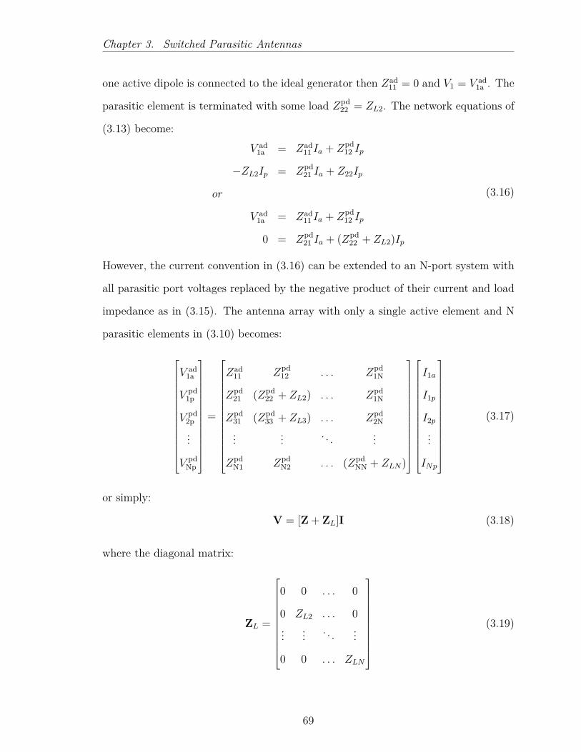
Chapter 3. Switched Parasitic Antennas
one active dipole is connected to the ideal generator then Zad11 = 0 and V1 = V ad
1a . The
parasitic element is terminated with some load Zpd22 = ZL2. The network equations of
(3.13) become:V ad
1a = Zad11 Ia + Zpd
12 Ip
−ZL2Ip = Zpd21 Ia + Z22Ip
or
V ad1a = Zad
11 Ia + Zpd12 Ip
0 = Zpd21 Ia + (Zpd
22 + ZL2)Ip
(3.16)
However, the current convention in (3.16) can be extended to an N-port system with
all parasitic port voltages replaced by the negative product of their current and load
impedance as in (3.15). The antenna array with only a single active element and N
parasitic elements in (3.10) becomes:
V ad1a
V pd1p
V pd2p...
V pdNp
=
Zad11 Zpd
12 . . . Zpd1N
Zpd21 (Zpd
22 + ZL2) . . . Zpd1N
Zpd31 (Zpd
33 + ZL3) . . . Zpd2N
... ... . . . ...
ZpdN1 Zpd
N2 . . . (ZpdNN + ZLN)
I1a
I1p
I2p
...
INp
(3.17)
or simply:
V = [Z + ZL]I (3.18)
where the diagonal matrix:
ZL =
0 0 . . . 0
0 ZL2 . . . 0... ... . . . ...
0 0 . . . ZLN
(3.19)
69

Chapter 3. Switched Parasitic Antennas
contains the load impedances terminated at each parasitic element.
Equation (3.18) has been well analyzed in parasitic arrays by Harrington [96], Mautz
and Harrington [119], and later by Dinger [120]. Any change in the loading configura-
tion of the parasitic elements only affect the load impedance matrix. Hence, ZL can
be calculated independently without making any amendments in the antenna array
design. According to (3.17), the values of self-impedances Zad11 and mutual-impedances
ZpdNN need to be calculated by considering the mutual coupling effect.
As already discussed in chapter 2 (section 2.8) of this thesis, the values of mutual
impedance between the active and parasitic elements and self-impedance of an an-
tenna can be calculated by using (2.28) and (2.31) and respectively. The MATLAB
simulation code function ‘impedmat’ is used for solving these impedances of the par-
asitic arrays is presented in the Appendix-B.
3.4 SPA System Description
In this thesis, a low-cost beam steering SPA is used to consider the radiation patterns
in the azimuth plane with an operating frequency of 2.4 GHz in the industrial, scien-
tific, and medical radio (ISM) band. The parasitic elements are terminated with load
impedance with the use of ideal RF switches. The switching between on/off states,
results in fixed radiation patterns in different directions.
When the RF switch is in the on state, the parasitic element is short-circuited and
acts as a reflector with an assumed theoretical value of the load impedance ≈ 10000 Ω.
When the RF switch is in the off state, parasitic element is open-circuited and act
as director and assumed with theoretical value of the impedance load ≈ 0Ω. As the
RF switches are assumed ideal, no insertion losses are considered in the calculation
of the impedance matrices.
70
Chapter 3. Switched Parasitic Antennas
The number of radiation patterns can be determined by the number of parasitic
elements and the switching load configurations of the parasitic elements. The perfor-
mance and functionality of using SPA depends on the basic principle of electromag-
netic mutual coupling. The design procedure of MIMO-SPA requires the structural
parameters of the antenna elements and the load configuration parameters terminated
on the parasitic elements [121]. The structural parameters of the antenna elements
include :
• Total number of elements (T=A+P), where T is the total number of the ele-
ments in the antenna array, A is the number of active elements and P is the
number of parasitic elements.
• The length of the active elements (lad);
• The length of the parasitic elements (lpd);
• The width of the elements, (W ); and
• The distance of the parasitic elements from the active elements, (d).
The load configuration parameters can be set as reactive loads or resistive loads.
The reactive loads with varactor diodes provide the tuning between the loads over
an infinite number of levels. The resistive loads can provide switching in fixed or
pre-defined levels.
In this thesis, the parasitic elements are terminated with impedance loads. The length
of the parasitic elements is the same in order to achieve omni-directional patterns [122].
An even number of parasitic elements is used to attain the antenna symmetry property
[121] [123]. However, the structural and load configurations can be optimized for the
better system performance. In the literature, most researchers have used optimization
algorithms and numerical analysis for the optimization purpose [124]. In this work,
71
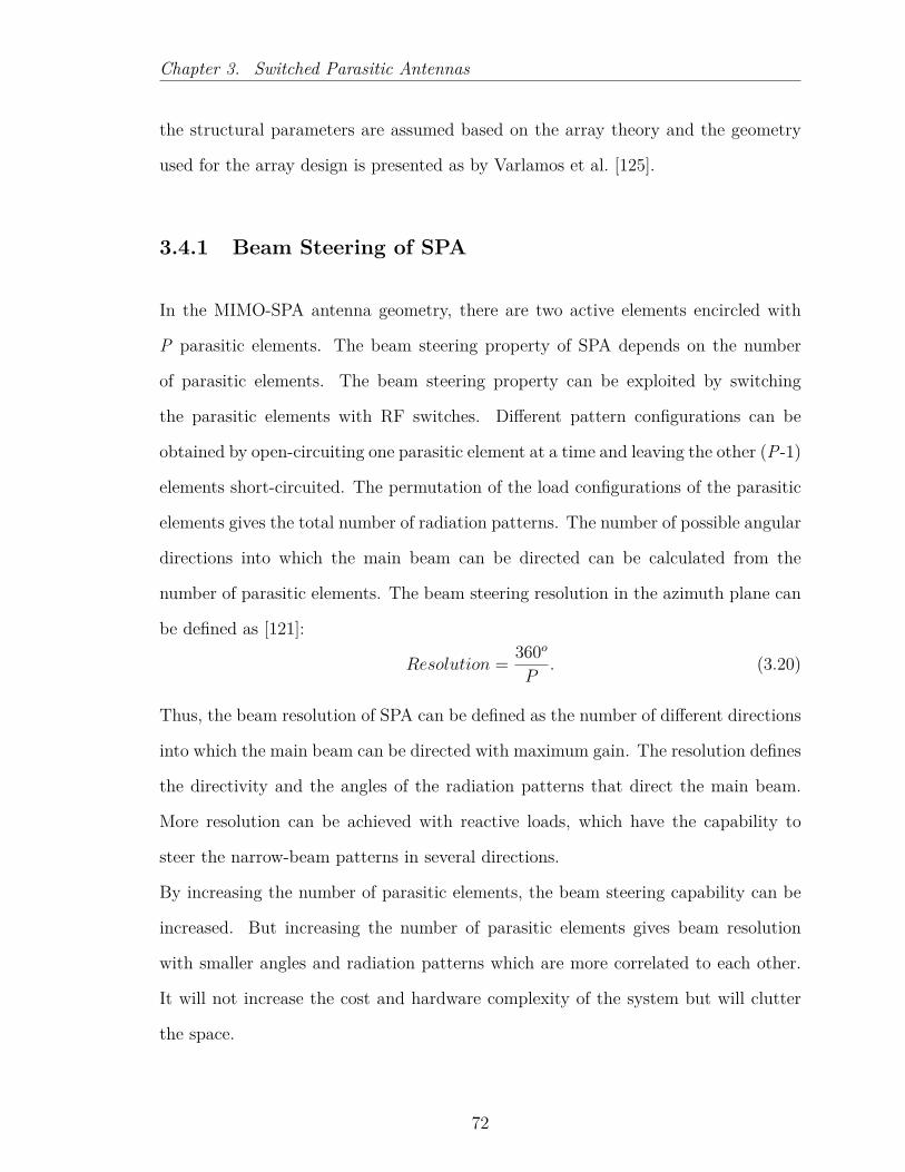
Chapter 3. Switched Parasitic Antennas
the structural parameters are assumed based on the array theory and the geometry
used for the array design is presented as by Varlamos et al. [125].
3.4.1 Beam Steering of SPA
In the MIMO-SPA antenna geometry, there are two active elements encircled with
P parasitic elements. The beam steering property of SPA depends on the number
of parasitic elements. The beam steering property can be exploited by switching
the parasitic elements with RF switches. Different pattern configurations can be
obtained by open-circuiting one parasitic element at a time and leaving the other (P-1)
elements short-circuited. The permutation of the load configurations of the parasitic
elements gives the total number of radiation patterns. The number of possible angular
directions into which the main beam can be directed can be calculated from the
number of parasitic elements. The beam steering resolution in the azimuth plane can
be defined as [121]:
Resolution = 360oP
. (3.20)
Thus, the beam resolution of SPA can be defined as the number of different directions
into which the main beam can be directed with maximum gain. The resolution defines
the directivity and the angles of the radiation patterns that direct the main beam.
More resolution can be achieved with reactive loads, which have the capability to
steer the narrow-beam patterns in several directions.
By increasing the number of parasitic elements, the beam steering capability can be
increased. But increasing the number of parasitic elements gives beam resolution
with smaller angles and radiation patterns which are more correlated to each other.
It will not increase the cost and hardware complexity of the system but will clutter
the space.
72

Chapter 3. Switched Parasitic Antennas
3.4.2 Loading Configurations
The number of radiation patterns not only depends on the number of parasitic ele-
ments but also on the switching capability of the load configurations. In this thesis,
with the use of RF switches, only two switching states on/off are possible with the
terminated load impedances.
Total number of pattern configurations = (Ls)P (3.21)
where P is the total number of the parasitic elements used in the single ring circular
SPA antenna array and Ls denotes possible values of the load impedances terminating
the parasitic elements.
All the loading configurations will provide different pattern configurations depending
on the loading values of the parasitic elements. These radiation patterns can be
selected with some objective function in terms of maximum gain or minimum insertion
loss.
3.5 SPA Performance Evaluation
SPA antennas with a smaller number of parasitic elements provides a limited number
of directions into which the main beam can be direct with maximum gain. The
number of directions can be increased with the switching configuration capability of
the loading configurations.
In the SPA evaluation performance, the radiation elements operate at a frequency of
2.4 GHz. The specification of the antenna elements are based on the antenna array
theory of half-wave dipoles, The length of the parasitic elements is changed with RF
switches to act as reflectors and directors as in the Yagi-Uda antenna.
73

Chapter 3. Switched Parasitic Antennas
3.5.1 Simulation Procedure
The beam-steering capability of SPA has been simulated with the MATLAB. Two
ideal RF switches are used with the on/off states i.e.(Ls = 2). In order to see
the mutual coupling effect on all the elements, the impedance matrix needs to be
calculated first. A change in the number of parasitic elements and the loading con-
figurations results in a change only in the loading matrix. The switching between
the controllable impedance loads changes the distribution of currents and radiation
patterns of the antenna array.
3.5.2 Testing Platforms
The case studies are as follows:
• Case-I. Loading configurations for the 4-Elements SPA geometry;
• Case-II. Loading configurations for the 6-Elements SPA geometry; and
• Case-III. Loading configurations for the 8-Elements SPA geometry.
3.5.2.1 Case-I. Loading configurations for the 4-Elements SPA antenna
geometry
The MIMO-SPA antenna geometry with total four elements consists of two active
elements and two parasitic elements as shown in Figure 3.6. The total loading con-
figurations with two switching levels (on/off) gives four (22 = 4) beam pattern con-
figurations.
74

Chapter 3. Switched Parasitic Antennas
Figure 3.6: Structure example of two active elements and two parasitic elements.
As shown in Table 3.1, there are total four pattern configurations denoted as (P1,
P2, P3, P4). The switching state of two parasitic elements (PE1, PE2) is represented
as open-circuited and short-circuited. When the RF switch is in the on-state, the
corresponding parasitic element is short-circuited and the load state is denoted by SC.
Whereas, when the RF switch is in the off -state, the corresponding parasitic element
is open-circuited or isolated from the ground plane and the load state is denoted by
OC. The theoretical impedance load values corresponding to the off -switch state is
≈ 10000 Ω and is represented in binary form as State=0. The load value corresponding
to on-switch state is ≈ 0 Ω and is represented in binary form as State=1.
Table 3.1: Pattern configurations using two parasitic elements
No. PE1 PE2 Pattern ConfigurationsP1 OC OC States=00P2 OC SC States=01P3 SC OC States=10P4 SC SC States=11
75

Chapter 3. Switched Parasitic Antennas
Figure 3.7 shows four different radiation pattern configurations with two active el-
ements and two parasitic elements. The first beam pattern configuration P1, when
both switches of the Parasitic Elements (PE) are in the off state shows (States=00),
in second beam pattern configuration P2 with PE1 in off state and PE2 in the on
state shows(States=01), in the third beam pattern configuration P3, with PE1 in on
state and PE2 in the off state shows (States=10), and in the last beam configuration
P4, with both PE1 and PE2 are in off states shows (States=11).
States=00
0.5
1
30
210
60
240
90
270
120
300
150
330
180 0
States=01
0.5
1
30
210
60
240
90
270
120
300
150
330
180 0
States=10
0.5
1
30
210
60
240
90
270
120
300
150
330
180 0
States=11
0.5
1
30
210
60
240
90
270
120
300
150
330
180 0
Figure 3.7: Radiation patterns with two active elements and two parasitic elements.
Table 3.2 shows the antenna parameters by using SPA configurations. Due to the
antenna symmetry property some of the parameters show same results.
Table 3.2: Antenna parameters with corresponding pattern configurations
Pattern Gain Zin Return Loss Reflection CoefficientNo. (dBi) (Ω) (dB) (Γ)P1 2.6150 87.0223 +73.2088i 12.7705 0.4323 + 0.3033iP2 2.2754 96.5057 +48.7038i 16.5941 0.3854 + 0.2043iP3 2.2754 96.5057 +48.7038i 16.5941 0.3854 + 0.2043iP4 2.0525 85.9698 +24.0628i 23.2049 0.2869 + 0.1262i
76
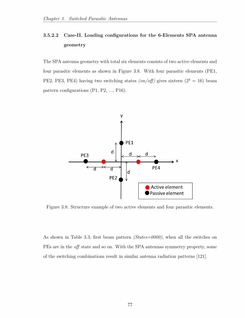
Chapter 3. Switched Parasitic Antennas
3.5.2.2 Case-II. Loading configurations for the 6-Elements SPA antenna
geometry
The SPA antenna geometry with total six elements consists of two active elements and
four parasitic elements as shown in Figure 3.8. With four parasitic elements (PE1,
PE2, PE3, PE4) having two switching states (on/off) gives sixteen (24 = 16) beam
pattern configurations (P1, P2, ..., P16).
Figure 3.8: Structure example of two active elements and four parasitic elements.
As shown in Table 3.3, first beam pattern (States=0000), when all the switches on
PEs are in the off state and so on. With the SPA antennas symmetry property, some
of the switching combinations result in similar antenna radiation patterns [121].
77

Chapter 3. Switched Parasitic Antennas
Table 3.3: Pattern configurations using four parasitic elements
No. PE1 PE2 PE3 PE4 Pattern ConfigurationsP1 OC OC OC OC States=0000P2 OC OC OC SC States=0001P3 OC OC SC OC States=0010P4 OC OC SC SC States=0011P5 OC SC OC OC States=0100P6 OC SC OC SC States=0101P7 OC SC SC OC States=0110P8 OC SC SC SC States=0111P9 SC OC OC OC States=1000P10 SC OC OC SC States=1001P11 SC OC SC OC States=1010P12 SC OC SC SC States=1011P13 SC SC OC OC States=1100P14 SC SC OC SC States=1101P15 SC SC SC OC States=1110P16 SC SC SC SC States=1111
Figure 3.9 shows sixteen different radiation pattern configurations with two active
elements and four parasitic elements.
78

Chapter 3. Switched Parasitic Antennas
States=0000
0.5
1
30
210
60
240
90
270
120
300
150
330
180 0
States=0001
0.5
1
30
210
60
240
90
270
120
300
150
330
180 0
States=0010
0.5
1
30
210
60
240
90
270
120
300
150
330
180 0
States=0011
0.5
1
30
210
60
240
90
270
120
300
150
330
180 0
States=0100
0.5
1
30
210
60
240
90
270
120
300
150
330
180 0
States=0101
0.5
1
30
210
60
240
90
270
120
300
150
330
180 0
States=0110
0.5
1
30
210
60
240
90
270
120
300
150
330
180 0
States=0111
0.5
1
30
210
60
240
90
270
120
300
150
330
180 0
States=1000
0.5
1
30
210
60
240
90
270
120
300
150
330
180 0
States=1001
0.5
1
30
210
60
240
90
270
120
300
150
330
180 0
States=1010
0.5
1
30
210
60
240
90
270
120
300
150
330
180 0
States=1011
0.5
1
30
210
60
240
90
270
120
300
150
330
180 0
States=1100
0.5
1
30
210
60
240
90
270
120
300
150
330
180 0
States=1101
0.5
1
30
210
60
240
90
270
120
300
150
330
180 0
States=1110
0.5
1
30
210
60
240
90
270
120
300
150
330
180 0
States=1111
0.5
1
30
210
60
240
90
270
120
300
150
330
180 0
Figure 3.9: Radiation patterns with two active elements and four parasitic elements.
Table 3.4 shows the antenna parameters by using SPA configurations. Due to the
antenna symmetry property some of the parameters show same results.
79

Chapter 3. Switched Parasitic Antennas
Table 3.4: Antenna parameters with corresponding pattern configurations
Pattern Gain Zin Return Loss Reflection CoefficientNo. (dBi) (Ω) (dB) (Γ)P1 2.6241 0.9151 + 0.5786i 15.2801 0.3946 + 0.2476iP2 2.1671 0.8952 + 0.5653i 15.6103 0.3843 + 0.2494iP3 2.1671 0.8952 + 0.5653i 15.6103 0.3843 + 0.2494iP4 2.2882 0.8691 + 0.5491i 16.0361 0.3708 + 0.2523iP5 2.1671 0.9500 + 0.6273i 14.3214 0.4191 + 0.2513iP6 2.6842 0.9278 + 0.6096i 14.6923 0.4076 + 0.2529iP7 2.7476 0.9306 + 0.6086i 14.6988 0.4081 + 0.2518iP8 2.6280 0.9017 + 0.5865i 15.1917 0.3929 + 0.2540iP9 2.1671 0.9500 + 0.6273i 14.3214 0.4191 + 0.2513iP10 2.7476 0.9306 + 0.6086i 14.6988 0.4081 + 0.2518iP11 2.6842 0.9278 + 0.6096i 14.6923 0.4076 + 0.2529iP12 2.6280 0.9017 + 0.5865i 15.1917 0.3929 + 0.2540iP13 2.2882 1.0027 + 0.7022i 13.0538 0.4538 + 0.2552iP14 2.6280 0.9801 + 0.6771i 13.4685 0.4413 + 0.2556iP15 2.6280 0.9801 + 0.6771i 13.4685 0.4413 + 0.2556iP16 2.5164 0.9503 + 0.6453i 14.0349 0.4244 + 0.2561i
3.5.2.3 Case-III. Loading configurations for the 8-Elements SPA antenna
geometry
In SPA antenna geometry with a total of eight elements, there are four active elements
and four parasitic elements as shown in Figure 3.10. The total load configurations
with two switching levels (on/off) gives four (24 = 16) beam pattern configurations.
Figure 3.11 shows the sixteen different beam configurations with four active elements
surrounded by four parasitic elements. There are four parasitic elements, the same as
shown in Table 3.3, with two switching levels (on/off), giving sixteen (24 = 16) beam
pattern configurations. Due to the SPA antenna’s symmetry property, some of the
combinations result in similar antenna radiation patterns [121].
80

Chapter 3. Switched Parasitic Antennas
Figure 3.10: Structure example of four active elements and four parasitic elements.
Table 3.5 shows the antenna parameters by using SPA configurations. Due to the
antenna symmetry property some of the parameters show same results.
Table 3.5: Antenna parameters with corresponding pattern configurations
Pattern Gain Zin Return Loss Reflection CoefficientNo. (dBi) (Ω) (dB) (Γ)P1 2.9565 2.1303 + 0.7381i 8.4599 0.6476 + 0.0989iP2 3.1229 0.9971 + 0.8081i 11.6796 0.4827 + 0.2792iP3 3.1229 0.9971 + 0.8081i 11.6796 0.4827 + 0.2792iP4 2.9137 0.6956 + 0.9448i 9.1410 0.4851 + 0.4069iP5 1.7264 1.0529 + 0.4764i 16.0015 0.4114 + 0.1806iP6 1.5181 0.8622 + 0.5944i 15.1705 0.3833 + 0.2691iP7 1.5181 0.8622 + 0.5944i 15.1705 0.3833 + 0.2691iP8 1.4798 0.8062 + 0.7541i 12.3378 0.4258 + 0.3315iP9 1.7264 0.7216 + 1.1079i 7.5636 0.5508 + 0.4074iP10 1.5181 0.6566 + 0.9106i 9.3152 0.4662 + 0.4202iP11 1.5181 0.6566 + 0.9106i 9.3152 0.4662 + 0.4202iP12 1.4798 0.5341 + 0.8758i 8.7153 0.4369 + 0.4769iP13 2.5668 0.6868 + 0.9541i 8.9744 0.4882 + 0.4114iP14 2.7955 0.6734 + 0.8418i 10.3790 0.4374 + 0.4036iP15 2.7955 0.6734 + 0.8418i 10.3790 0.4374 + 0.4036iP16 2.8682 0.5917 + 0.8234i 10.0206 0.4162 + 0.4404i
81

Chapter 3. Switched Parasitic Antennas
States=0000
0.5
1
30
210
60
240
90
270
120
300
150
330
180 0
States=0001
0.5
1
30
210
60
240
90
270
120
300
150
330
180 0
States=0010
0.5
1
30
210
60
240
90
270
120
300
150
330
180 0
States=0011
0.5
1
30
210
60
240
90
270
120
300
150
330
180 0
States=0100
0.5
1
30
210
60
240
90
270
120
300
150
330
180 0
States=0101
0.5
1
30
210
60
240
90
270
120
300
150
330
180 0
States=0110
0.5
1
30
210
60
240
90
270
120
300
150
330
180 0
States=0111
0.5
1
30
210
60
240
90
270
120
300
150
330
180 0
States=1000
0.5
1
30
210
60
240
90
270
120
300
150
330
180 0
States=1001
0.5
1
30
210
60
240
90
270
120
300
150
330
180 0
States=1010
0.5
1
30
210
60
240
90
270
120
300
150
330
180 0
States=1011
0.5
1
30
210
60
240
90
270
120
300
150
330
180 0
States=1100
0.5
1
30
210
60
240
90
270
120
300
150
330
180 0
States=1101
0.5
1
30
210
60
240
90
270
120
300
150
330
180 0
States=1110
0.5
1
30
210
60
240
90
270
120
300
150
330
180 0
States=1111
0.5
1
30
210
60
240
90
270
120
300
150
330
180 0
Figure 3.11: Radiation patterns with four active elements and four parasitic elements.
3.6 Conclusion
This chapter has presented a low-cost beam-steering antenna based on parasitic ele-
ments that can steer the beam pattern into a fixed number of directions. The pattern
diversity property is exploited with the use of parasitic elements. The antenna ele-
ments have been analyzed with N-port network theory. The mutual coupling effect
forms the foundation of the operation between the antenna elements and is repre-
82

Chapter 3. Switched Parasitic Antennas
sented with the calculation of impedance matrices. The impedance matrices provide
the current distribution on each antenna element. The current redistribution alters
the radiation pattern of the antenna array. Different radiation pattern configuration
are obtained by changing the structural geometry of SPA and the loading configura-
tions of the parasitic elements.
83

Chapter 4
MIMO Channel Capacity Analysis
using Switched Parasitic Antennas
In this chapter, the main consideration is to achieve spatial multiplexing gain in the
MIMO system using parasitic elements at the receiver side, where size, cost, power and
complexity are the primary constraints. The design is basically intended to exploit
pattern diversity by using the parasitic elements. It consists of few active elements
coupled to set of parasitic elements terminated with impedance loads. By switching
the impedance loads, the radiation patterns can be configured into different angular
positions. It gives the flexibility to the receiver to sense information from various
portions of the space. The influence of the covariance matrix is also shown in the
calculation of channel capacity for various pattern configurations. This covariance
matrix shows upper bounds on the channel capacity with the antenna selection and
proper power allocation techniques.
84
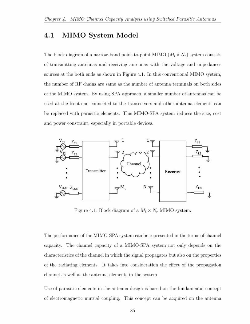
Chapter 4. MIMO Channel Capacity Analysis using Switched Parasitic Antennas
4.1 MIMO System Model
The block diagram of a narrow-band point-to-point MIMO (Mt×Nr) system consists
of transmitting antennas and receiving antennas with the voltage and impedances
sources at the both ends as shown in Figure 4.1. In this conventional MIMO system,
the number of RF chains are same as the number of antenna terminals on both sides
of the MIMO system. By using SPA approach, a smaller number of antennas can be
used at the front-end connected to the transceivers and other antenna elements can
be replaced with parasitic elements. This MIMO-SPA system reduces the size, cost
and power constraint, especially in portable devices.
Figure 4.1: Block diagram of a Mt ×Nr MIMO system.
The performance of the MIMO-SPA system can be represented in the terms of channel
capacity. The channel capacity of a MIMO-SPA system not only depends on the
characteristics of the channel in which the signal propagates but also on the properties
of the radiating elements. It takes into consideration the effect of the propagation
channel as well as the antenna elements in the system.
Use of parasitic elements in the antenna design is based on the fundamental concept
of electromagnetic mutual coupling. This concept can be acquired on the antenna
85

Chapter 4. MIMO Channel Capacity Analysis using Switched Parasitic Antennas
terminals with the use of impedance matrices. Figure 4.2 depicts the MIMO-SPA
model using antenna impedances ZTT and ZRR at the transmitting and the receiving
sides respectively. To find out the effect of the antenna terminals on the MIMO
channel capacity, it is necessary to consider the mutual coupling effect and calculate
the impedance matrices using the antenna parameters.
Figure 4.2: MIMO-SPA system with impedance matrices at both link ends.
Based on N-port theory, the voltage and current relationship between the transmit
and the receive arrays can be represented as [115] :
VT
VR
=
ZTT ZTR
ZRT ZRR
IT
IR
(4.1)
where
VT = [VT1, VT2, ..., VTMt]T is voltage source vector at the transmitting end,
iT = [IT1, IT2, ..., ITMt]T is the current vector at the transmitting end,
VR = [VR1, VR2, ..., VRNr]T is voltage source vector at the receiver end,
86

Chapter 4. MIMO Channel Capacity Analysis using Switched Parasitic Antennas
iR = [IR1, IR2, ..., IRNr]T is the currents vector at the receiver end.
The diagonal matrices ZTT and ZRR are the self-impedance matrices at the transmit-
ting and receiving antennas receptively. ZTR and ZRT are mutual-impedance matrices
between transmitting and receiving antennas.
These voltage and current sources can be represented by means of Thevenin’s theorem
where an ideal voltage source VSi is connected in series with source impedance ZSi
as [86]:
VS = IS(ZTT + ZS) (4.2)
The currents at the transmitter side can be obtained as:
IS = (ZTT + ZS)−1VS (4.3)
where IS = [IS1IS2...ISMt ]T , VS = [VS1VS2...VSMt ]
T and ZS = diag(ZS1ZS2...ZSMt).
Consider the parameter G relating the current at the transmitter side to the voltage
at the receiver side. The parameter G also includes the electromagnetic effect of the
propagation environment. The voltage-current relationship at the receiver side with
the propagation effects can be denoted as:
VO = GIS (4.4)
At the receiver side, the output voltage with impedance matrices including antenna
impedance matrix and loading matrix can be obtained as:
VO = (ZRR + ZL)IR (4.5)
87
Chapter 4. MIMO Channel Capacity Analysis using Switched Parasitic Antennas
or (4.5) can be written in the current form as:
IR = (ZRR + ZL)−1VO (4.6)
where ZL = diag(ZL1ZL2...ZLNr) is the diagonal loading impedance and ZRR is the
antenna impedance matrix of the receiving array. On the receiver side, the voltage-
current relationship in terms of the receiving impedance of the antennas can be written
as:
VR = ZRR(IR) (4.7)
From (4.6), (4.7) can be re-written as:
VR = ZRR(ZRR + ZL)−1VO (4.8)
The relationship between the voltage at the source side VS and at the receiver side
VR can be described as:
VR = ZRR(ZRR + ZL)−1G(ZTT + ZS)−1VS = HVS (4.9)
With (4.9), it is easy to evaluate the voltage at the receiver side by calculating
impedance matrices ZTT and ZRR at the transmitter and receiver sides respectively.
These impedance matrices consider the effect of electromagnetic mutual coupling ex-
ists between the antenna terminals. The effect of the parasitic elements can also be
realized with source impedance matrix ZS at the transmitter side and with the load-
ing impedance matrix ZL at the receiver side. The number of parasitic elements can
be changed independently at the transmitter and receiver sides. The loading effect
at the transmitter and at the receiver side changes the source impedance ZS and the
loading impedance ZL respectively.
88

Chapter 4. MIMO Channel Capacity Analysis using Switched Parasitic Antennas
These parasitic elements are the passive elements and are not connected to any RF
source. Thus, it is not possible to access the voltages directly on the parasitic elements.
The voltage can be obtained at the active elements by using permutation matrices as
follows:
VR = SRHVS (4.10)
where SR is a permutation matrix of dimensions (Nra×Nr), Nra represents the number
of active elements at the receiver side. It extracts the voltage at the active elements
induced by the parasitic elements. Thus, the permutation matrix at the receiver side
extracts the values of H that are relative to the active elements.
If the parasitic elements are connected at the transmitter side, the information across
the parasitic elements can be accessed with the permutation matrix ST. The per-
mutation matrix ST has dimensions (Mt ×Mta), where Mta is the number of active
elements at the transmitter side. With the use of permutation matrices ST and SR
at the transmitter and receiver sides respectively, (4.10) can be written as:
VR = SRHSTVS = HVS (4.11)
or
H = SRHST (4.12)
The effect of the parasitic elements can be realized with these permutation matrices
ST and SR, which select the rows and columns of H relative to the active elements
connected to the transceivers.
89

Chapter 4. MIMO Channel Capacity Analysis using Switched Parasitic Antennas
4.2 Modelling the Effect of the Parasitic Elements
4.2.1 MIMO Channel Matrix (H) using SPA
The effect of the transmitting and receiving antenna terminals can be evaluated in
terms of the impedance matrices. The impedance loads of the parasitic elements can
also be represented in the form of matrices. The MIMO channel can be represented in
the form of a channel matrix (H) including antenna impedances matrices and loading
parasitic elements matrices on both sides in the equation form as [7]:
H = ZRR(ZRR + ZL)−1G(ZTT + ZS)−1 (4.13)
where G is the propagation channel matrix including the effect of channel patterns
and the scatterers. This modelling effect of the parasitic elements can be represented
with a channel matrix at the transmitter and at the receiver side separately.
Consider a transmitting array with transmitting elements (Mt), with active elements
(Mta) and parasitic elements (Mtp), so that the total elements at the transmitter side
are (Mt = Mta+Mtp). With any change in the number of active and parasitic elements,
(4.13) will be unchanged, only the values of the diagonal matrix ZS will change in
order to model the parasitic impedance loads at the transmitter side.
Equation (4.13) can be rewritten when parasitic elements are used at the transmitter
side only:
Htp = (ZRR + ZL)−1G(ZTT + ZS,Mtp)−1ST (4.14)
where the subscript tp stands for parasitic elements at the transmitting side.
Equation (4.14) is similar to (4.13), the only change being the loading impedances
terminating the parasitic elements in ZS.
Similarly to the transmitter side, parasitic elements can be used at the receiver side
90

Chapter 4. MIMO Channel Capacity Analysis using Switched Parasitic Antennas
as well. Consider a receiving array with active elements (Nra) and parasitic elements
(Nrp), so that the total elements are (Nr = Nra + Nrp). Again, (4.13) will be un-
changed, only the values of the diagonal matrix ZL will change in order to model the
parasitic impedance loads at the receiver side. Equation (4.13) can be rewritten when
parasitic elements are used at the receiver side only:
Hrp = SR(ZRR + ZL,Nrp)−1G(ZTT + ZS)−1 (4.15)
where the subscript rp stands for parasitic elements at the receiving side.
The complete channel matrix with parasitic elements at both sides can be evaluated
as [7]:
Htp,rp = SR(ZRR + ZL,rp)−1G(ZTT + ZS,tp)−1ST (4.16)
where the subscripts tp, rp represent the parasitic elements on the transmitting and
receiving sides respectively. The permutation matrices ST and SR select the coeffi-
cients of H relative to the active elements connected to the transceivers.
Equation (4.16) shows the modification in the channel matrix by using parasitic el-
ements at the transmitter and the receiver sides. Any modification in the loading
impedance values of the parasitic elements can be realized in the form of the channel
matrix. Hence, the effect of parasitic elements in the matrices ZS,tp and ZL,rp, can
change the coefficients of the channel matrix and can also vary the channel capacity.
It should be noted that the relationship between Htp,rp and the loading impedances
ZS,tp and ZL,rp, is non-linear because of the matrix inversion.
In this thesis, parasitic elements are used only at the receiver side for simplicity, thus
changing the loads of impedance matrix ZL,rp only. It is also possible to change the
parasitic controlling impedances at the transmitter side ZS,tp such as at a base station
but it will make significant impact on all the users at the receiver side.
91

Chapter 4. MIMO Channel Capacity Analysis using Switched Parasitic Antennas
4.2.2 MIMO Channel Capacity using SPA
The channel realizations in a MIMO-SPA system change with the use of parasitic
elements. To evaluate the channel capacity in MIMO-SPA, it is necessary to consider
the parameters of the channel matrix H.
In flat-fading MIMO systems, the channel matrix depends on the system architec-
ture and the particular channel propagation conditions. The coefficients of H can
be considered with some probability distribution. With a large number of scatterers,
the channel matrix coefficients can be assumed with zero-mean Gaussian distribution
random variables. In the ideal case, when all the channel coefficients are uncorre-
lated, the highest channel capacity can be achieved. This is only possible in the case
of rich scattering propagation environments, where the signals at the receiver are
uncorrelated.
In MIMO systems, the transmitted symbol vector s transmits input symbol (s =
s1, s2...sMt) individually from transmit antennas (Mt) and the output can be defined
as:
y =√EsMt
Hs + n (4.17)
where n = (n1, n2, ...nNr) is a noise vector and is assumed to consists of zero-mean,
circular symmetric, complex Gaussian random variables. The autocorrelation of the
transmitted signal vector can be defined as: Rss = EssH. Assume transmit power
across each antenna is 1, such as Tr(Rss) = Mt.
When CSI is available at the transmitter, the decomposition model gives information
about the possible number of spatial links possible in the given MIMO system. By
using SVD, it converts the multiple equations of the MIMO system into equivalent
spatial links. The transmitter is pre-processed with V and the receiver signal is post-
92

Chapter 4. MIMO Channel Capacity Analysis using Switched Parasitic Antennas
processed with UH .
The output of the MIMO system (4.17) can be written by using SVD as:
y =√EsMt
UHHVs + n (4.18)
Using the SVD model, the number of MIMO channels is divided into a number of
independent SISO channels. The channel matrix H ∈ CMt×Nr with SVD can be
represented as:
H = UΣVH (4.19)
where U ∈ CNr×Nr and V ∈ CMt×Mt are unitary matrices and Σ ∈ CMt×Nr is a
rectangular matrix. The off-diagonal elements of Σ are zero and the diagonal ele-
ments of Σ are non-zero. These are known as singular values and can be denoted as
(λ1, λ2, ...λmin), where Nmin , min(Mt, Nr). The rank parameter of H represents the
non-zero singular values, such that rank(H) ≤ Nmin.
Thus, Shannon’s channel capacity [126] of MIMO system can be evaluated as :
C =r∑i=1
log2
(1 + αiPtσi
2
N0
)(bit/s/Hz) (4.20)
where Pt is the total transmitted power, σ2i is the ith singular value of the matrix H, r
is the rank of the matrix H, N0 is the noise variance at the receiver, and αi shows the
percentage of the transmitted power on the sub-channels. Equation(4.20) shows that
the MIMO channel capacity depends on the singular values of the channel matrix H.
93

Chapter 4. MIMO Channel Capacity Analysis using Switched Parasitic Antennas
4.3 MIMO Channel Capacity Analysis with Dif-
ferent Pattern Configurations
Conventional MIMO, gives only one channel matrix realization with the dimensions
of the transmitting and receiver antenna elements. By using parasitic elements, there
will be different channel realizations of the channel matrices depending on the loading
configurations. The number of loading configurations can be calculated from the
number of parasitic elements and the level of impedance loads terminated on them.
To see the effect of the parasitic elements on the MIMO channel capacity, it is nec-
essary to obtain the channel matrix using (4.16) to evaluate Htp,rp. In this thesis,
parasitic elements are only used at the receiver side, thus there is need to calculate
Hrp only, as in (4.15).
The MIMO channel capacity can be evaluated by using Shannon’s theory as follows
[126]:
C = E
maxTr(Rss)=Mt
log2 det(INr + Es
MtN0HrpRssHrp
H
) (4.21)
where Es is the total transmitted power, N0 is the variance of the additive white
Gaussian noise at the receiver, Hrp represents the channel matrix using parasitic
elements at the receiver side only, Rss represents the covariance matrix and must be
determined to satisfy the transmitter power constraints.
Compared to the traditional MIMO system, instead of finding the channel capacity
for only one channel matrix, MIMO-SPA exploits the pattern diversity and provides a
number of channel matrices. With the different load impedances across the parasitic
elements, there will be different realizations of the channel matrices. The number
of channel matrices depends on the number of parasitic elements and the available
switching levels across the parasitic elements.
94

Chapter 4. MIMO Channel Capacity Analysis using Switched Parasitic Antennas
4.3.1 MIMO-SPA (2× 2) using two Parasitic Elements
As discussed in chapter 3, section (3.4) showed SPA performance evaluation to create
radiation patterns in three different cases. MIMO-SPA (2 × 2) using two parasitic
elements represent the Case-I, where parasitic elements are used only at the receiver
side. For the simulation purpose, the arrangement of array elements is same as shown
in Figure 3.6.
Simulation scenario for MIMO-SPA system (Mt×Nr) using two parasitic elements at
the receiver side only:
• Number of active elements at transmitter side Mta=2
• Number of active elements at receiver side Nra=2
• Number of parasitic elements at transmitter side Mtp=0
• Number of parasitic elements at receiver side Nrp=2
• Total number of elements at the transmitter side M = Mta +Mtp=2+0=2
• Total number of elements at the receiver side N = Nra +Nrp=2+2=4
In MIMO-SPA with (2×2) dimensions, using two parasitic elements gives four different
channel matrices (CH00,CH01,CH10,CH11) according to the state of the switches
(on/off). The channel matrix (CH00) represents with both the parasitic elements
are in the off state, which is similar to the conventional MIMO without using any
parasitic elements.
Figure 4.3, shows the channel capacity with four different pattern configurations.
The beam pattern configuration (CH00) shows the same channel capacity same as
conventional MIMO (2 × 2) when there are only active elements present. In this
95

Chapter 4. MIMO Channel Capacity Analysis using Switched Parasitic Antennas
uncorrelated propagation environment simulation scenario, the channel coefficients
of the four pattern configurations are uncorrelated in each case. Figure 4.3 shows
that channel matrix (CH10) provides the highest channel capacity among the other
pattern configurations.
0 2 4 6 8 10 12 14 16 18 20SNR [dB]
0
2
4
6
8
10
12
Erg
odic
Cha
nnel
Cap
acit
y (b
ps/H
z)
CH00CH01CH10CH11
Figure 4.3: MIMO-SPA (2× 2) with two parasitic elements.
The conventional MIMO (2 × 2) using only active elements gives average channel
capacity 4.1 bit/s/Hz. MIMO-SPA (2× 2) using two parasitic elements increases the
average channel capacity to 5.3 bit/s/Hz. The simulation results show that by using
parasitic elements, it is possible to increase the channel capacity.
96

Chapter 4. MIMO Channel Capacity Analysis using Switched Parasitic Antennas
4.3.2 MIMO-SPA (2× 2) using four Parasitic Elements
Case-II in section (3.4), represents MIMO-SPA (2× 2) using four parasitic elements.
The arrangement of array elements at the receiver side is same as shown in Figure
3.8.
Simulation scenario for MIMO system (Mt×Nr) using four parasitic elements at the
receiver side only :
• Number of active elements at transmitter side Mta=2
• Number of active elements at receiver side Nra=2
• Number of parasitic elements at transmitter side Mtp=0
• Number of parasitic elements at receiver side Nrp=4
• Total number of elements at the transmitter side M = Mta +Mtp=2+0=2
• Total number of elements at the receiver side N = Nra +Nrp=2+4=6
MIMO-SPA with (2 × 2) using four parasitic elements gives a total of sixteen (24 =
16) channel matrices (CH0000,CH0001, ...,CH1111) for sixteen different beam pattern
configurations. As shown in Figure 4.4, pattern configuration (States=0000), when
all the switches on PEs are in the off state is equivalent to the conventional MIMO
with only active elements are present. Due to the SPA antennas symmetry property,
some of the pattern configurations shows similar results for ergodic channel capacity.
Figure 4.4 depicts the ergodic channel capacity in the uncorrelated propagation sce-
nario for the sixteen pattern configurations. The simulation results show that the
channel matrix (CH1101) provides the highest channel capacity among all the other
pattern configurations.
97

Chapter 4. MIMO Channel Capacity Analysis using Switched Parasitic Antennas
0 2 4 6 8 10 12 14 16 18 20SNR[dB]
0
2
4
6
8
10
12
14
Erg
odic
Chan
nel
Cap
acit
y (
bps/
Hz)
CH0000CH0001CH0010CH0011CH0100CH0101CH0110CH0111CH1000CH1001CH1010CH1011CH1100CH1101CH1110CH1111
Figure 4.4: MIMO-SPA (2× 2) with four parasitic elements.
In comparison conventional MIMO (2×2) using only active elements shows an average
channel capacity of 5.3 bit/s/Hz and MIMO-SPA (2×2) using four parasitic elements
increases the average channel capacity to 5.7 bit/s/Hz. The simulation results show
improvement in the MIMO channel capacity by using parasitic elements with low-
hardware complexity in the communication systems.
98

Chapter 4. MIMO Channel Capacity Analysis using Switched Parasitic Antennas
4.3.3 MIMO-SPA (4× 4) using four Parasitic Elements
Case-III in section (3.4), represents MIMO-SPA (4× 4) using four parasitic elements.
The arrangement of array elements where four active elements are surrounded with
four parasitic elements is same as shown in Figure 3.10.
Simulation scenario for MIMO-SPA system (Mt × Nr) using four parasitic elements
at the receiver side only :
• Number of active elements at transmitter side Mta=4
• Number of active elements at receiver side Nra=4
• Number of parasitic elements at transmitter side Mtp=0
• Number of parasitic elements at receiver side Nrp=4
• Total number of elements at the transmitter side M = Mta +Mtp=4+0=4
• Total number of elements at the receiver side N = Nra +Nrp=4+4=8
Figure 4.5 shows MIMO-SPA (4×4) with four parasitic elements. Using four parasitic
elements at the receiver side gives sixteen different beam pattern configurations. Four
parasitic elements with two switching levels (on/off) gives sixteen (24 = 16) pattern
configurations corresponding to sixteen channel matrices (CH0000,CH0001, ...,CH1111).
The first beam pattern (States=0000), when all the switches of PEs are in the off state
is equivalent to conventional MIMO with active elements only. In the uncorrelated
propagation scenario, the channel matrix (CH1101) provides the highest channel ca-
pacity among all the other pattern configurations.
In a comparison of MIMO-SPA with standard MIMO, MIMO (4 × 4) using only
active elements gives an average channel capacity of 8.5 bit/s/Hz, while MIMO-SPA
99

Chapter 4. MIMO Channel Capacity Analysis using Switched Parasitic Antennas
0 2 4 6 8 10 12 14 16 18 20
SNR[dB]
0
2
4
6
8
10
12
14
16
18
20
Erg
odic
Chan
nel
Cap
acit
y (
bps/
Hz)
CH0000CH0001CH0010CH0011CH0100CH0101CH0110CH0111CH1000CH1001CH1010CH1011CH1100CH1101CH1110CH1111
Figure 4.5: MIMO-SPA (4× 4) with four parasitic elements.
(4×4) using four parasitic elements gives an average channel capacity of 9.2 bit/s/Hz.
Thus, the simulation results show that the addition of parasitic elements provides low-
complexity and higher channel capacity in MIMO systems.
4.4 MIMO System with Covariance Matrix
MIMO performance relies on the characteristics of the channel matrix and the avail-
ability of CSI on both sides of the communication link. At the receiver, it is possible to
estimate this information by using channel estimation techniques with pilot training
symbols. Often, the receiver feeds back this information to the transmitter. Instead of
sending all this information, the receiver can send only the statistics of the channel in
100

Chapter 4. MIMO Channel Capacity Analysis using Switched Parasitic Antennas
the form of the covariance matrix. The advantage of using this information is that the
statistics of the channel changes slowly as compared to the realization of the channel
itself. MIMO-SPA channel capacity can be evaluated by using Shannon’s theory as
follows [126]:
C = E
maxTr(Rss)=Mt
log2 det(INr + Es
MtN0HrpRssHrp
H
) (4.22)
where Rss is the covariance matrix, which defines the presence of correlation in the
propagation environment. If knowledge of the covariance matrix is available at the
transmitter, it can distribute the power accordingly to the sub-channels.
The covariance matrix can be modified by using two techniques, IAST and WPA:
• IAST technique selects the subset of transmit antennas according to their con-
tribution to the MIMO channel capacity. The antenna that contributes most to
the channel capacity is selected first and then another antenna with the second
highest contribution and so on. Thus, the selection process of antennas is in
increasing order at the transmitter side.
• WPA technique allocates power to the selected antennas at the transmitter side.
When CSI is available, WPA allocates the transmit power across all the transmit
antennas in an optimal way. If the channel information is not available at the
transmitter side then the optimal way is to distribute the power uniformly across
all the transmit antennas.
The covariance matrix can be evaluated for these two techniques and can be defined
as [18]:
RImpss = VRopt
ss VH (4.23)
where Roptss = γopt1 , γopt2 ...γoptMt
is the optimal covariance matrix and V is the unitary
101

Chapter 4. MIMO Channel Capacity Analysis using Switched Parasitic Antennas
matrix that satisfies V HV = IQ.
Hence, the improved channel capacity in MIMO-SPA according to the optimal covari-
ance matrix is given by:
CImp = E
maxRss
log2 det(INr + Es
MtN0HrpRImp
ss HrpH
) (4.24)
4.4.1 Influence of Covariance Matrix
The covariance matrix shows the correlation present in the channel matrix H. The
characteristics of the covariance matrix change according to the distribution of the
channel-coefficients. Variation in the power allocation on the MIMO transmit anten-
nas also makes changes in the correlation matrix. Hence, this effect can be analyzed in
terms of channel capacity. The influence of the covariance matrix (Rss), with power
constraints developed by [127] and has been used in [18] [128]:
Rss(α) = αI + (1− α)uuH (4.25)
where u = [11...1]T , I is the identity matrix and α is a real number with power
constraint which satisfies 0 ≤ α ≤ PP−1 .
• when α=0, then Rss(0) = uuH which shows that the covariance matrix Rss
has all elements of its matrix with value of 1. This means that all the channel
coefficients correlated.
• when α = 1, then Rss(1) = I which shows that the covariance matrix Rss has
all its elements are uncorrelated.
• when α parameter distributes power in the optimal way, it gives the improved
correlation matrix. Thus, Rss(opt) = Rss(Imp).
102

Chapter 4. MIMO Channel Capacity Analysis using Switched Parasitic Antennas
4.4.2 MIMO-SPA Channel Capacity with Different Covari-
ance Matrices
MIMO-SPA channel capacity also shows impact on different pattern configurations
with the improved covariance matrix. With the knowledge of these matrices, it is
possible to evaluate Shannon’s channel capacity as follows [126]:
CImp = E
maxRss
log2 det(INr + Es
MtN0HrpRImp
ss HrpH
) (4.26)
The covariance matrix Rss needs to be determined to satisfy the transmitter power
constraints. The covariance matrix can change the channel capacity across all the
pattern configurations according to the power allocation at the transmitter side by
using SVD. With the different realizations of the channel matrices, the MIMO channel
capacity will be different across each pattern configuration. The more the channels
are correlated, the lower will be the channel capacity and vice-versa.
4.5 MIMO-SPA Channel Capacity with IAST and
WPA
When the channel conditions are known at the transmitter, the antenna can select
the subset of antennas with incremental/decremental antenna selection techniques.
The power allocation can be carried with WPA at the transmitter side.
In this thesis, incremental antenna selection technique (IAST) is used to select the
best set of antennas at the transmitter side and power is allocated in an optimal way
by using WPA. The variation in the channel capacity can be evaluated with different
covariance matrices that change the power allocation at the transmitter side. The
103

Chapter 4. MIMO Channel Capacity Analysis using Switched Parasitic Antennas
comparison is discussed with three different covariance matrices as follows:
• IAST with correlated covariance matrix-[Rss]corr
• IAST with uncorrelated covariance matrix- [Rss]uncorr
• IAST with improved covariance matrix using WPA- [Rss]WPA
4.5.1 MIMO-SPA (2× 2) using two Parasitic Elements
4.5.1.1 IAST with correlated covariance matrix- [Rss]corr
In the correlated case, when there is correlation present in the covariance matrix
[Rss]corr, all the elements of the matrix are set to one as in (4.25) with α = 0 . This
means that all the channel coefficients are correlated. The covariance matrix accord-
ing to (4.25) can be represented as Rss(0) or [Rss]corr .
Figure 4.6 shows the ergodic channel capacity across four pattern configurations with
IAST and the correlated covariance matrix [Rss]corr. The ergodic channel capacity
does not show significant increase with respect to SNR. Due to the high correlation
present between the channel coefficients, covariance matrix [Rss]corr represents a neg-
ative influence on the channel capacity.
104

Chapter 4. MIMO Channel Capacity Analysis using Switched Parasitic Antennas
0 2 4 6 8 10 12 14 16 18 20
SNR [dB]
0
1
2
3
4
5
6
Erg
odic
Chan
nel
Cap
acit
y (
bps/
Hz)
CH00 CorrelatedCH01 CorrelatedCH10 CorrelatedCH11 Correlated
Figure 4.6: MIMO-SPA (2 × 2) channel capacity using two parasitic elements withmatrix of all ones as correlation matrix.
4.5.1.2 IAST with uncorrelated covariance matrix- [Rss]uncorr
In the uncorrelated case, the covariance matrix [Rss]uncorr is an identity matrix. The
diagonal elements of the matrix are ones and all other elements are zeros as in (4.25)
with α = 1 . This means that all the channel coefficients are uncorrelated. The
covariance matrix according to (4.25) can be represented as Rss(1). For the proper
allocation of the power, IAST is used to select the antennas in particular order.
Figure 4.7 shows the ergodic channel capacity increases with respect to SNR in the
uncorrelated case. The channel matrix (CH10) provides the highest channel capacity
among all the other pattern configurations.
105

Chapter 4. MIMO Channel Capacity Analysis using Switched Parasitic Antennas
0 2 4 6 8 10 12 14 16 18 20SNR [dB]
0
2
4
6
8
10
12
Erg
odic
Cha
nnel
Cap
acit
y (b
ps/H
z)
CH00 UncorrelatedCH01 UncorrelatedCH10 UncorrelatedCH11 Uncorrelated
Figure 4.7: MIMO-SPA (2 × 2) channel capacity using two parasitic elements withidentity matrix as correlation matrix.
4.5.1.3 IAST with improved covariance matrix using WPA- [Rss]WPA
The improved covariance matrix is obtained by selecting the best set of antennas
using IAST and then allocating optimal power using WPA. The improved covariance
matrix is represented as Rss(Imp).
The comparison of four different pattern configurations for correlated [Rss]corr, uncor-
related [Rss]uncorr and improved covariance using WPA [Rss]WPA is shown in Figure
4.8. For all the parasitic configurations, the MIMO channel capacity is improved with
the power allocation using WPA as compared to the equal power distribution across
all the transmit antennas.
106

Chapter 4. MIMO Channel Capacity Analysis using Switched Parasitic Antennas
0 2 4 6 8 10 12 14 16 18 20SNR [dB]
0
2
4
6
8
10
12
Erg
odic
Chan
nel
Cap
acit
y (
bps/
Hz)
CH00 WPACH00 UncorrelatedCH00 CorrelatedCH01 WPACH01 UncorrelatedCH01 CorrelatedCH10 WPACH10 UncorrelatedCH10 CorrelatedCH11 WPACH11 UncorrelatedCH11 Correlated
Figure 4.8: Comparison of the channel capacity using the three different methods forMIMO-SPA (2× 2) using two parasitic elements.
The comparison of channel capacity for each beam pattern configuration can be plot-
ted separately. Figure 4.9 shows the comparison for all the four channel matrices
(CH00,CH01,CH10,CH11) with different covariance matrices. In each plot of chan-
nel matrix, the ergodic channel capacity performance improves with the covariance
matrix using WPA [Rss]WPA.
From Figure 4.9, the proposed system shows improvement from 4.9 bit/s/Hz of the
conventional MIMO (2 × 2) to 5.3 bit/s/Hz in MIMO-SPA (2 × 2) using only two
parasitic elements. Thus, the selection of best antennas with the optimal strategy of
power allocation provides a higher channel capacity.
107

Chapter 4. MIMO Channel Capacity Analysis using Switched Parasitic Antennas
0 2 4 6 8 10 12 14 16 18 20SNR[dB]
0
2
4
6
8
10
12
Ch
an
nel
Cap
acit
y (
bp
s/H
z)
CH00 WPACH00 UncorrelatedCH00 Correlated
0 2 4 6 8 10 12 14 16 18 20
SNR[dB]
0
2
4
6
8
10
12
Ch
an
nel
Cap
acit
y (
bp
s/H
z)
CH01 WPACH01 UncorrelatedCH01 Correlated
0 2 4 6 8 10 12 14 16 18 20
SNR[dB]
0
2
4
6
8
10
12
Ch
an
nel
Cap
acit
y (
bp
s/H
z)
CH10 WPACH10 UncorrelatedCH10 Correlated
0 2 4 6 8 10 12 14 16 18 20
SNR[dB]
0
2
4
6
8
10
12
Ch
an
nel
Cap
acit
y (
bp
s/H
z)
CH11 WPACH11 UncorrelatedCH11 Correlated
Figure 4.9: Comparison of the channel capacity using the three different methods forMIMO-SPA (2× 2) using two parasitic elements.
4.5.2 MIMO-SPA (2× 2) using four Parasitic Elements
4.5.2.1 IAST with correlated covariance matrix- [Rss]corr
Figure 4.10 shows the comparison for all the sixteen channel matrices
(CH0000,CH0001, ...,CH1111) with the correlated covariance matrix [Rss]corr. In this
case, all the channel coefficients of the MIMO-SPA channel matrices for all the sixteen
configurations are correlated. The ergodic channel capacity for IAST is decreased for
all the pattern configurations when the covariance matrix is correlated.
108

Chapter 4. MIMO Channel Capacity Analysis using Switched Parasitic Antennas
0 2 4 6 8 10 12 14 16 18 20SNR[dB]
1
2
3
4
5
6
7
8
9
Erg
odic
Chan
nel
Cap
acit
y (
bps/
Hz)
CH0000 CorrelatedCH0001 CorrelatedCH0010 CorrelatedCH0011 CorrelatedCH0100 CorrelatedCH0101 CorrelatedCH0110 CorrelatedCH0111 CorrelatedCH1000 CorrelatedCH1001 CorrelatedCH1010 CorrelatedCH1011 CorrelatedCH1100 CorrelatedCH1101 CorrelatedCH1110 CorrelatedCH1111 Correlated
Figure 4.10: MIMO-SPA (2× 2) channel capacity using four parasitic elements withmatrix of all ones as correlation matrix.
4.5.2.2 IAST with uncorrelated covariance matrix- [Rss]uncorr
Figure 4.11 shows the comparison for all the sixteen channel matrices
(CH0000,CH0001, ...,CH1111) with the identity matrix I as the covariance matrix.
In this case, all the channel coefficients of the MIMO-SPA channel matrices for all the
sixteen configurations are uncorrelated. Figure 4.11 shows the pattern configuration
(CH1101) provides the highest ergodic channel capacity as compared to all the other
pattern configurations.
109

Chapter 4. MIMO Channel Capacity Analysis using Switched Parasitic Antennas
0 2 4 6 8 10 12 14 16 18 20
SNR[dB]
0
2
4
6
8
10
12
14
Erg
odic
Chan
nel
Cap
acit
y (
bps/
Hz)
CH0000 UncorrelatedCH0001 UncorrelatedCH0010 UncorrelatedCH0011 UncorrelatedCH0100 UncorrelatedCH0101 UncorrelatedCH0110 UncorrelatedCH0111 UncorrelatedCH1000 UncorrelatedCH1001 UncorrelatedCH1010 UncorrelatedCH1011 UncorrelatedCH1100 UncorrelatedCH1101 UncorrelatedCH1110 UncorrelatedCH1111 Uncorrelated
Figure 4.11: MIMO-SPA (2× 2) channel capacity using four parasitic elements withidentity matrix as correlation matrix.
4.5.2.3 IAST with improved covariance matrix using WPA- [Rss]WPA
The comparison of channel capacity for each beam pattern configuration for
MIMO-SPA (2 × 2) channel capacity using four parasitic elements can be plotted
separately. Figure 4.12 shows the comparison for all the sixteen channel matrices
(CH0000,CH0001,CH0010, ...,CH1111) with different covariance matrices. In each
plot of channel matrix, the ergodic channel capacity performance improves with the
covariance matrix using WPA [Rss]WPA.
110

Chapter 4. MIMO Channel Capacity Analysis using Switched Parasitic Antennas
0 5 10 15 20SNR[dB]
0
5
10
15C
hannel
Capacit
y (
bps/H
z)
CH0000 WPACH0000 UncorrelatedCH0000 Correlated
0 5 10 15 20
SNR[dB]
0
5
10
15
Channel
Capacit
y (
bps/H
z)
CH0001 WPACH0001 UncorrelatedCH0001 Correlated
0 5 10 15 20
SNR[dB]
0
5
10
15
Channel
Capacit
y (
bps/H
z)
CH0010 WPACH0010 UncorrelatedCH0010 Correlated
0 5 10 15 20
SNR[dB]
0
5
10
15
Channel
Capacit
y (
bps/H
z)
CH0011 WPACH0011 UncorrelatedCH0011 Correlated
0 5 10 15 20
SNR[dB]
0
5
10
15
Channel
Capacit
y (
bps/H
z)
CH0100 WPACH0100 UncorrelatedCH0100 Correlated
0 5 10 15 20
SNR[dB]
0
5
10
15
Channel
Capacit
y (
bps/H
z)
CH0101 WPACH0101 UncorrelatedCH0101 Correlated
0 5 10 15 20
SNR[dB]
0
5
10
15
Channel
Capacit
y (
bps/H
z)
CH0110 WPACH0110 UncorrelatedCH0110 Correlated
0 5 10 15 20
SNR[dB]
0
5
10
15
Channel
Capacit
y (
bps/H
z)
CH0111 WPACH0111 UncorrelatedCH0111 Correlated
0 5 10 15 20
SNR[dB]
0
5
10
15
Channel
Capacit
y (
bps/H
z)
CH1000 WPACH1000 UncorrelatedCH1000 Correlated
0 5 10 15 20
SNR[dB]
0
5
10
15
Channel
Capacit
y (
bps/H
z)
CH1001 WPACH1001 UncorrelatedCH1001 Correlated
0 5 10 15 20
SNR[dB]
0
5
10
15
Channel
Capacit
y (
bps/H
z)
CH1010 WPACH1010 UncorrelatedCH1010 Correlated
0 5 10 15 20
SNR[dB]
0
5
10
15
Channel
Capacit
y (
bps/H
z)
CH1011 WPACH1011 UncorrelatedCH1011 Correlated
0 5 10 15 20
SNR[dB]
0
5
10
15
Channel
Capacit
y (
bps/H
z)
CH1100 WPACH1100 UncorrelatedCH1100 Correlated
0 5 10 15 20
SNR[dB]
0
5
10
15
Channel
Capacit
y (
bps/H
z)
CH1101 WPACH1101 UncorrelatedCH1101 Correlated
0 5 10 15 20
SNR[dB]
0
5
10
15
Channel
Capacit
y (
bps/H
z)
CH1110 WPACH1110 UncorrelatedCH1110 Correlated
0 5 10 15 20
SNR[dB]
0
5
10
15
Channel
Capacit
y (
bps/H
z)
CH1111 WPACH1111 UncorrelatedCH1111 Correlated
Figure 4.12: Comparison of the channel capacity using the three different methodsfor MIMO-SPA (2× 2) using four parasitic elements.
Simulation results show that the conventional MIMO gives the channel capacity of 5.8
bit/s/Hz. It increases with improved covariance matrix to 6.2 bit/s/Hz in MIMO-SPA
with four parasitic elements. Hence, the optimal covariance matrix with the proper
selection of antenna with the optimal power allocation improves the channel capacity
significantly.
111

Chapter 4. MIMO Channel Capacity Analysis using Switched Parasitic Antennas
4.5.3 MIMO-SPA (4× 4) using four Parasitic Elements
4.5.3.1 IAST with correlated covariance matrix- [Rss]corr
Figure 4.13 shows the comparison for all the sixteen channel matrices
(CH0000,CH0001, ...,CH1111) with the correlated covariance matrix [Rss]corr. In this
case, all the channel coefficients of the MIMO channel matrices for all the sixteen
configurations are correlated. The ergodic channel capacity for IAST is decreased for
all the pattern configurations when the covariance matrix is correlated.
0 2 4 6 8 10 12 14 16 18 20SNR[dB]
0
1
2
3
4
5
6
7
8
Erg
odic
Chan
nel
Cap
acit
y (
bps/
Hz)
CH0000 CorrelatedCH0001 CorrelatedCH0010 CorrelatedCH0011 CorrelatedCH0100 CorrelatedCH0101 CorrelatedCH0110 CorrelatedCH0111 CorrelatedCH1000 CorrelatedCH1001 CorrelatedCH1010 CorrelatedCH1011 CorrelatedCH1100 CorrelatedCH1101 CorrelatedCH1110 CorrelatedCH1111 Correlated
Figure 4.13: MIMO-SPA (4× 4) channel capacity using four parasitic elements withmatrix of all ones as correlation matrix.
112

Chapter 4. MIMO Channel Capacity Analysis using Switched Parasitic Antennas
4.5.3.2 IAST with uncorrelated covariance matrix- [Rss]uncorr
Figure 4.14 shows the comparison for all the sixteen channel matrices
(CH0000,CH0001, ...,CH1111) with the identity matrix as the covariance matrix. In
this case, all the channel coefficients of the MIMO channel matrices for all the sixteen
configurations are uncorrelated. Figure 4.14 shows the pattern configuration (CH1110)
provides the highest ergodic channel capacity as compared to all the other pattern
configurations. It also shows the improvement by using SPA with MIMO as compared
to the conventional MIMO without parasitic elements.
0 2 4 6 8 10 12 14 16 18 20SNR[dB]
0
2
4
6
8
10
12
14
16
18
20
Erg
odic
Chan
nel
Cap
acit
y (
bps/
Hz)
CH0000 UncorrelatedCH0001 UncorrelatedCH0010 UncorrelatedCH0011 UncorrelatedCH0100 UncorrelatedCH0101 UncorrelatedCH0110 UncorrelatedCH0111 UncorrelatedCH1000 UncorrelatedCH1001 UncorrelatedCH1010 UncorrelatedCH1011 UncorrelatedCH1100 UncorrelatedCH1101 UncorrelatedCH1110 UncorrelatedCH1111 Uncorrelated
Figure 4.14: MIMO-SPA (4× 4) channel capacity using four parasitic elements withidentity matrix as correlation matrix.
113

Chapter 4. MIMO Channel Capacity Analysis using Switched Parasitic Antennas
4.5.3.3 IAST with improved covariance matrix using WPA- [Rss]WPA
The comparison of channel capacity for each beam pattern configuration for MIMO
(4× 4) using four parasitic elements can be plotted separately. Figure 4.15 shows the
comparison for all the sixteen channel matrices (CH0000,CH0001,CH0010, ...,CH1111)
with different covariance matrices. In each plot of channel matrix, the ergodic channel
capacity performance improves with the covariance matrix using WPA [Rss]WPA.
0 5 10 15 20SNR[dB]
0
5
10
15
20
Channel
Capacit
y (
bps/H
z)
CH0000 WPACH0000 UncorrelatedCH0000 Correlated
0 5 10 15 20
SNR[dB]
0
5
10
15
20
Channel
Capacit
y (
bps/H
z)
CH0001 WPACH0001 UncorrelatedCH0001 Correlated
0 5 10 15 20
SNR[dB]
0
5
10
15
20
Channel
Capacit
y (
bps/H
z)
CH0010 WPACH0010 UncorrelatedCH0010 Correlated
0 5 10 15 20
SNR[dB]
0
5
10
15
20
Channel
Capacit
y (
bps/H
z)
CH0011 WPACH0011 UncorrelatedCH0011 Correlated
0 5 10 15 20
SNR[dB]
0
5
10
15
20
Channel
Capacit
y (
bps/H
z)
CH0100 WPACH0100 UncorrelatedCH0100 Correlated
0 5 10 15 20
SNR[dB]
0
5
10
15
20
Channel
Capacit
y (
bps/H
z)
CH0101 WPACH0101 UncorrelatedCH0101 Correlated
0 5 10 15 20
SNR[dB]
0
5
10
15
20
Channel
Capacit
y (
bps/H
z)
CH0110 WPACH0110 UncorrelatedCH0110 Correlated
0 5 10 15 20
SNR[dB]
0
5
10
15
20
Channel
Capacit
y (
bps/H
z)
CH0111 WPACH0111 UncorrelatedCH0111 Correlated
0 5 10 15 20
SNR[dB]
0
5
10
15
20
Channel
Capacit
y (
bps/H
z)
CH1000 WPACH1000 UncorrelatedCH1000 Correlated
0 5 10 15 20
SNR[dB]
0
5
10
15
20
Channel
Capacit
y (
bps/H
z)
CH1001 WPACH1001 UncorrelatedCH1001 Correlated
0 5 10 15 20
SNR[dB]
0
5
10
15
20
Channel
Capacit
y (
bps/H
z)
CH1010 WPACH1010 UncorrelatedCH1010 Correlated
0 5 10 15 20
SNR[dB]
0
5
10
15
20
Channel
Capacit
y (
bps/H
z)
CH1011 WPACH1011 UncorrelatedCH1011 Correlated
0 5 10 15 20
SNR[dB]
0
5
10
15
20
Channel
Capacit
y (
bps/H
z)
CH1100 WPACH1100 UncorrelatedCH1100 Correlated
0 5 10 15 20
SNR[dB]
0
5
10
15
20
Channel
Capacit
y (
bps/H
z)
CH1101 WPACH1101 UncorrelatedCH1101 Correlated
0 5 10 15 20
SNR[dB]
0
5
10
15
20
Channel
Capacit
y (
bps/H
z)
CH1110 WPACH1110 UncorrelatedCH1110 Correlated
0 5 10 15 20
SNR[dB]
0
5
10
15
20
Channel
Capacit
y (
bps/H
z)
CH1111 WPACH1111 UncorrelatedCH1111 Correlated
Figure 4.15: Comparison of the channel capacity using the three different methodsfor MIMO-SPA (4× 4) using four parasitic elements.
114

Chapter 4. MIMO Channel Capacity Analysis using Switched Parasitic Antennas
Simulation results show that conventional MIMO gives a channel capacity of 9.1
bit/s/Hz, increasing with improved covariance matrix to 9.8 bit/s/Hz with MIMO-
SPA with four parasitic elements. The optimal covariance matrix with the proper
selection of antennas and optimal power allocation improves the channel capacity.
4.6 MIMO-SPA Channel Capacity with correla-
tion matrix
In MIMO-SPA, the variation in the correlation matrix shows changes in the channel
capacities for all the pattern configurations as shown in Figure 4.9, Figure 4.12 and
Figure 4.15. Upper and lower bounds on channel capacity with the influence of
covariance matrix in three different cases with (4.25) can be represented as:
• when α=0 then [Rss]corr = Cmin, which gives lower-bounds on the channel
capacity with all the coefficients of the channel matrix for each pattern config-
uration are correlated.
• when α = 1 then [Rss]uncorr = Cmax, which gives channel capacity with all the
coefficients of the channel matrix for each pattern configuration are uncorrelated.
The channel capacity shows better results than correlated environment.
• when α parameter allocates power in optimal way with IAST and WPA, it gives
the improved correlation matrix. Thus, [Rss]Imp = CImp, shows upper-bounds
on the channel capacity.
115

Chapter 4. MIMO Channel Capacity Analysis using Switched Parasitic Antennas
The comparison of channel capacity (4.26) with respect to the covariance matrix Rss
can be represented as:
Cmin = C∣∣∣∣Rss(0)
(4.27)
Cmax = C∣∣∣∣Rss(1)
(4.28)
CImp = C∣∣∣∣Rss(Imp)
(4.29)
Therefore, lower and upper bounds for the channel capacity can be established with
the corresponding correlation matrices as follows:
Cmin ≤ Cmax ≤ CImp (4.30)
Equation (4.30) shows a lower-bound on the channel capacity Cmin with the correlated
covariance matrix [Rss]corr or Rss(0). An intermediate channel capacity Cmax achieved
with the uncorrelated covariance matrix [Rss]uncorr or Rss(1). An upper-bound on
channel capacity CImp obtained with the optimal covariance matrix [Rss]Imp. These
channel capacity bounds show the influence of the covariance matrix with variations
of the power parameter in MIMO-SPA systems.
4.7 Conclusion
MIMO-SPA presented in this chapter is capable of steering beam patterns in different
directions by switching the parasitic elements. The use of pattern diversity is exploited
with parasitic elements that use the electromagnetic mutual coupling principle. This
effect on antenna elements is calculated by considering the impedance matrices. The
effect of radiating elements and propagation medium is evaluated to find out the
MIMO-SPA performance in terms of channel capacity. The ergodic channel capacity
116

Chapter 4. MIMO Channel Capacity Analysis using Switched Parasitic Antennas
have been calculated on all the pattern configurations. The influence of the correlation
matrix on the channel capacity is also shown with IAST and WPA. The simulation
results shows that the improved covariance matrix gives the upper bounds on the
channel capacity in the MIMO-SPA systems. Hence, the most cost-efficient MIMO
system is obtained by using IAST for the antenna subset selection and WPA for the
optimal power allocation across all the transmit antennas.
117

Chapter 5
Pattern Configuration Selection
This chapter investigates the MIMO-SPA system behavior based on the statistical
properties of the propagation environment. An overview of some important MIMO
channel quality metrics such as condition number and channel capacity are presented
in this chapter. A condition number is a channel quality indicator that represents
the correlation present in the MIMO channel. This chapter proposes a novel optimal
pattern configuration method based on channel statistics that can be sent back to the
transmitter with a low-rate feedback link. The optimal pattern configuration based
on the condition number at different SNR is also presented for different MIMO-SPA
scenarios.
5.1 Exploiting CSI at the Transmitter Side
MIMO technology provides promising solutions for the increasing demands of high
channel capacity and reliability in wireless communication systems. These advantages
are possible with knowledge of channel fading at both ends of the communication
link. In TDD systems, both links can exploit this information with the reciprocity
118

Chapter 5. Pattern Configuration Selection
principle. In FDD systems, both links use different radio frequencies and do not follow
the channel reciprocity principle.
Generally, the receiver can access the CSI by using channel estimation techniques but
it is not possible for the transmitter to access its own channels by direct means. It
relies on the receiver to get this information through the feedback channel. Thus, the
receiver first estimates the channel parameters by using pilot symbols then feeds back
this information to the transmitter.
In wireless communication systems, the main drawback is the requirement of an ad-
ditional resource to provide this information back to the transmitter. The amount of
feedback information also increases with the number of antennas used in the system.
Due to the feedback requirements in terms of system bandwidth, it is not practically
feasible to send full information on the channel to the transmitter. In time-varying
channel conditions, it is not possible for the transmitter to track the channel com-
pletely. The information also become outdated when the transmitter uses it for the
next transmission. At the transmitter, instead of sending the full CSI, statistical
knowledge of the channel can be exploited. It reduces the feedback overhead and is
updated only when there is significant change in the propagation channel.
The statistics of the changing environment can be sent back in the form of correlation
matrices. Another approach to sending partial information of the channel status is
to use the condition number of the channel matrix. A condition number reflects the
eigenvalue spread of the MIMO channel. It gives indication of the multipath richness
present in the given channel realization.
In long-term evolution (LTE), three indicators are used for the feedback purpose:
rank indicator (RI), precoding matrix indicator (PMI) and channel quality indicator
(CQI). The first two indicators are used for MIMO operation. CQI is the most
important indicator for scheduling and link adaptation purposes. The adaptation of
119

Chapter 5. Pattern Configuration Selection
the transmit signal to the channel variations improves the transmission rate of the
system. This adaptation in the MIMO systems is possible with the availability of CSI
at the transmitter by indirect means such as with channel estimation techniques and
with a reliable feedback link.
5.2 Importance of Channel Quality Metrics
In adaptive MIMO systems, the transmitter tracks the changes in the channel with the
information provided by the receiver. As shown in Figure 5.1, the receiver estimates
the channel with channel estimation techniques and sends back the low-rate feedback
link to the transmitter. The transmitter uses this information to adapt the channel
such as in terms of modulation and coding schemes for the next signal transmission.
Figure 5.1: Feedback link with CSI
When CSI is not available at the transmitter, the best policy is to allocate the trans-
mit power uniformly across all the transmit antennas. When the CSI is available at
the transmitter, the optimal power is allocated based on the quality of the channel.
The power allocation at the transmitter side is based on the eigenvalue spread of
the channel. The eigenvalue spread indicates the correlation present in the multi-
path propagation channel. It signifies the orthogonality present between the spatial
120

Chapter 5. Pattern Configuration Selection
channels. A low eigenvalue spread indicates that there is low correlation present in
the channel, which increases the spatial multiplexing gain. A high eigenvalue spread
indicates similarity between the spatial channels and provides limited or sometimes
only one channel, as in the beamforming technique [47].
In the high SNR regime, a greater channel capacity can be achieved with low eigen-
value spread. In the low SNR regime, most or all of the power is allocated to the
strongest eigenmode only. For high channel capacity or high spatial multiplexing gain,
it is desirable to have low eigenvalue spread.
5.2.1 MIMO Channel Condition Number
In MIMO systems, EVS indicates the degree of correlation present in multipath chan-
nel. The rank indicator indicates the number of spatial links possible to provide the
spatial multiplexing gain in the MIMO system. It only gives the information about
the possible number of spatial channels but does not give any information about the
quality of the spatial channels. Another channel metric is known as the condition
number, which gives an indication about the quality of the channel. It characterizes
the channel matrix in terms of the sensitivity of the channel matrix.
If the eigenvalues of the channel matrix are almost equal or the difference between the
eigenvalues is very low, it will provide a low condition number. This is also known
as a “well-conditioned channel” matrix. In the ideal case, with a rich-scattering
environment, where all the channels are uncorrelated, the MIMO channel matrix
provides the highest rank and the condition number is equal or close to 0 dB. This
indicates the orthogonality of the sub-channels and provides comparable channel gains
in different spatial directions. Due to the poor channel conditions with correlated
channels, the rank of the channel matrix drops to zero and is known as a rank-deficient
121
Chapter 5. Pattern Configuration Selection
channel matrix. The condition number of this channel matrix will be very high and
it will be difficult to properly recover the MIMO signal. Thus, the condition number
indicates whether the MIMO channel is capable of supporting spatial multiplexing
in MIMO systems. It is also used as a short-term indication of the SNR required to
properly recover a MIMO transmission.
As previously discussed in the literature [129] [130], a condition number can be defined
in a number of ways:
• The condition number can be defined as the ratio of the largest eigenvalue(λmax)
to the smallest eigenvalue (λmin). It can be obtained through eigenvalue decom-
position (EVD) and can be represented as:
κ = λmax(H)λmin(H) . (5.1)
The condition number can also be defined as the ratio of the largest singular
value (σmax) to the smallest singular value (σmin), where (σ) is obtained via the
SVD of the matrix. The eigenvalue and SVD produce the same result only when
the matrix is both symmetric and positive definite.
• Another method of finding the condition number is by the product of the norms
of the matrix and its inverse, such as: κ = ‖H‖.‖H−1‖, where ‖ denotes the
2-norm and is referred as the Euclidean distance.
In matrix theory [19], the condition number indicates how sensitive the solution of the
system is relative to its input. It tells about the stability of the system. If the channel
matrix is an “ill-conditioned” matrix, it will show drastic changes in the output data
with the small changes in the input. Thus, the system will be more prone to errors
and sensitive to channel noise and other interference issues.
122
Chapter 5. Pattern Configuration Selection
In an industrial publication [131], the relation between the condition number and its
effect on the throughput is discussed as shown in Table 5.1. The channel condition
number should be less than (≤ 19dB) to obtain the high throughput. With the high
correlation (≥ 19dB) between the channels, MIMO would not be able to increase
the throughput of the system. For the maximum throughput, the channels should
be totally independent with minimum correlation. Thus, the quality of the MIMO
system channel plays a vital role to optimizing the throughput of the LTE-A Downlink
Physical Layer.
Table 5.1: Channel condition number and its indications
Condition Number Indication
0dB Totally independent channels, Ideal condition toachieve maximum throughput
≤ 13dB Favorable condition which enables higher throughputas compare to SIMO/MISO
13dB-19dB Medium Correlation which provides marginalthroughput improvement
≥ 19dB High correlation where MIMO would not be able toincrease throughput
In the literature, the condition number has been used as a selection criterion for several
purposes in MIMO systems. Many studies [30] [33] have used the condition number
for switching between the diversity and spatial multiplexing schemes. Reconfigurable
patch antennas use the condition number to select the antenna configuration [34].
The adaptive MIMO transmission techniques [35] have used the condition number to
exploit the spatial selectivity of the wireless channels. Other research [36], demon-
strates the use of the regular condition number to evaluate the quality of the channel
matrix, as it provides some intuition on channel quality.
123

Chapter 5. Pattern Configuration Selection
5.2.2 MIMO Channel Capacity
According to the Shannon’s theorem [126], the MIMO channel capacity not only
changes with SNR and bandwidth, it also depends on the status of the channel matrix.
The quality of the channel matrix is also an important factor to evaluate the MIMO
channel capacity [132].
Figure 5.2 depicts the relation between SNR and the condition number. It shows how
the quality of the channel in terms of condition number decides the requirement for
the SNR in the system. For example, for the requirement of a channel capacity of
6 bits/s/Hz, a condition number of 0 dB requires a SNR of 9 dB. As the condition
number increases to 16 dB, it requires a SNR of 12 dB. For a condition number of 30
dB, it needs SNR of 15 dB for the same system data rate.
0 5 10 15 20 25 30 35 40Condition Number (dB)
0
5
10
15
20
25
30
35
SN
R (
dB)
Capacity=2Bits/s/HzCapacity=4Bits/s/HzCapacity=6Bits/s/HzCapacity=8Bits/s/HzCapacity=10Bits/s/HzCapacity=12Bits/s/Hz
Figure 5.2: Signal-to-noise ratio and condition number
124

Chapter 5. Pattern Configuration Selection
This shows that as the condition number increases, the system requires more SNR to
achieve the same performance. Figure 5.2 shows that the same performance can be
achieved even with low SNR values when the channel has a low condition number.
However, the condition number represents the correlation present in the channel co-
efficients in the channel matrix. The greater the correlation between the coefficients,
the higher will be the condition number. This correlation depends on a number of
factors including: small antenna spacing, common antenna polarization and a narrow
angular spread with a poor scattering environment.
The relationship between correlation and channel capacity in terms of cumulative
distribution function (cdf) is shown in Figure 5.3.
0 1 2 3 4 5 6 7 8 9 10Capacity (bits/s/Hz)
0
0.1
0.2
0.3
0.4
0.5
0.6
0.7
0.8
0.9
1
cdf
Low CorrelationMedium CorrelationHigh Correlation
Figure 5.3: CDF for the CN as a function of correlation between the channel coeffi-cients
Figure 5.3 shows the condition number in a MIMO system with low, medium and
125

Chapter 5. Pattern Configuration Selection
high correlation between antenna elements. The lower the correlation between the
channel coefficients, the higher the channel capacity will be and vice-versa. Thus,
as the correlation increases, the channel capacity decreases. The condition number
also represents the spatial selectivity of the channel in terms of the eigenvalue spread.
A greater eigenvalue spread provides a larger difference between the maximum and
minimum eigenvalues. This results in high condition number.
The relation between channel capacity and condition number with fixed SNR is shown
in Figure 5.4. It illustrates that as the condition number increases, the channel
capacity decreases. For example, to gain a channel capacity of 8 bits/s/Hz for a
condition number of 1 dB, requires a SNR of 10 dB. As the condition number increases
to 5 dB, it raises the requirement for the SNR to 20 dB. Thus, it shows that to achieve
the same performance with the increase in condition number, the system requires more
SNR.
0 2 4 6 8 10 12 14 16 18 20Condition Number(dB)
1
2
3
4
5
6
7
8
9
10
11
12
Erg
odic
Cap
acity
(bp
s/H
z)
SNR=1dBSNR=5dBSNR=10dBSNR=20dBSNR=30dB
Figure 5.4: Channel capacity with varying SNR
126

Chapter 5. Pattern Configuration Selection
Figure 5.5 depicts the behavior of condition number on the channel capacity with the
changing SNR values. It illustrates that at the ergodic capacity of 6 bits/s/Hz, with
low correlation or at lowest condition number of 1 dB, it requires SNR around 4 dB.
For the highest correlation, with condition number 30 dB, it requires the SNR of 19
dB. It is evident that as the channel condition number increases the MIMO channel
capacity decreases. Hence, the channels with low condition number or the highly
uncorrelated channels yields high MIMO channel capacity.
0 2 4 6 8 10 12 14 16 18 20SNR(dB)
1
2
3
4
5
6
7
8
9
10
11
Erg
odic
Cap
acity
(bp
s/H
z)
CN=1dBCN=5dBCN=10dBCN=20dBCN=30dB
Figure 5.5: Channel capacity with varying Condition Number
5.3 Pattern Configuration Selection using CN
A traditional MIMO system provides the channel matrix with only one channel re-
alization. In MIMO-SPA, the use of parasitic elements samples the electromagnetic
field over a much wider space. It provides freedom with the availability of a number
127

Chapter 5. Pattern Configuration Selection
of different channel realizations. Instead of increasing the number of active elements
to increase the spatial multiplexing gain, it is possible to achieve this through the use
of switching parasitic elements loaded with impedance loads.
MIMO-SPA with a number of switchable parasitic elements provides the structure
with different radiation patterns. These parasitic elements acts as scatterers sur-
rounded by the active elements. By changing the switching levels of the impedance
loads, in an on/off manner, the parasitic elements act in and out of resonance and
can modify the radiation patterns. With the optimal pattern configuration, they can
modify the overall radiation pattern of the system [7].
The condition number can be used as the objective function to select the best pattern
configuration from all the available pattern configurations. With this optimal selec-
tion objective, it is possible to adapt the antenna patterns to the prevailing channel
conditions.
Selection criterion using CN
Best Pattern Configuration = min(CN)P (5.2)
where P represents the total number of pattern configurations in MIMO-SPA.
The condition number can be used as the channel quality metric and can be fed back
to the transmitter with fewer bits. It gives information on the optimal channel state
and can reduce the feedback overhead in MIMO systems.
As discussed in chapter 3 section (3.5.2), three cases with different SPA geometries
provide different pattern configurations. To find the optimal pattern configuration,
CN is used as the selection criterion for all three cases.
128

Chapter 5. Pattern Configuration Selection
5.3.1 Configuration Selection for MIMO-SPA (2 × 2) using
two Parasitic Elements
MIMO-SPA (2× 2) with two parasitic elements at the receiver side provides four dif-
ferent pattern configurations as shown in Figure 3.7. All four pattern configurations
with four different channel matrix realizations (CH00,CH01,CH10,CH11) gives dif-
ferent condition numbers. By doing an exhaustive search, selecting the channel matrix
with (5.2) gives the minimum value of the condition number.
Table 5.2 shows the simulation results for the uncorrelated scenario. It gives the
pattern configuration matrix CH10 with the minimum condition number. This is the
optimal pattern configuration with the best channel quality and provides a higher
channel capacity than the other configurations.
Table 5.2: Pattern configurations of MIMO-SPA (2× 2) using two parasitic elements
No. Pattern Configurations Condition Number (dB)P1 CH00 2.20 6.84P2 CH01 3.61 11.14P3 CH10 1.94 5.78P4 CH11 3.12 9.88
5.3.2 Configuration Selection for MIMO-SPA (2 × 2) using
four Parasitic Elements
MIMO-SPA (2× 2) using four parasitic elements at the receiver side provides sixteen
different pattern configurations with different channel realizations as shown in Figure
3.9. All sixteen pattern configurations represent the sixteen different channel matrices
(CH0000,CH0001, ...,CH1111) with dimensions (2 × 2) and having different condition
numbers. By doing an exhaustive search, the best pattern configuration is selected
129

Chapter 5. Pattern Configuration Selection
with (5.2), which has the minimum condition number.
Table 5.3 shows the simulation results for the uncorrelated scenario. It gives the
pattern configuration matrix CH1000 as having the minimum condition number. This
is the optimal pattern configuration in this simulation scenario, with the best channel
quality, and provides a higher channel capacity than the other pattern configurations.
Table 5.3: Pattern configurations of MIMO-SPA (2× 2) using four parasitic elements
No. Pattern Configurations Condition Number (dB)P1 CH0000 3.97 11.98P2 CH0001 4.47 13.00P3 CH0010 4.46 12.99P4 CH0011 4.95 13.88P5 CH0100 4.19 12.44P6 CH0101 4.82 13.66P7 CH0110 4.60 13.25P8 CH0111 5.19 14.30P9 CH1000 3.29 10.34P10 CH1001 3.53 10.95P11 CH1010 3.90 11.82P12 CH1011 4.16 12.38P13 CH1100 3.47 10.80P14 CH1101 3.75 11.49P15 CH1110 4.00 12.05P16 CH1111 4.29 12.64
5.3.3 Configuration Selection for MIMO-SPA (4 × 4) using
four Parasitic Elements
MIMO-SPA (4× 4) using four parasitic elements at the receiver side provides sixteen
different pattern configurations with different channel realizations as shown in Figure
3.11. All sixteen pattern configurations represent the sixteen different channel matri-
ces (CH0000,CH0001...CH1111) with dimensions (4×4) and having different condition
130

Chapter 5. Pattern Configuration Selection
numbers. By doing an exhaustive search, the best pattern configuration is selected
with (5.2), which has the minimum condition number.
Table 5.4 shows the simulation results for the uncorrelated scenario. It gives the
pattern configuration matrix CH0111 as having the minimum condition number. It is
the optimal pattern configuration in this simulation scenario, with the best channel
quality, and provides a higher channel capacity than the other pattern configurations.
Table 5.4: Pattern configurations of MIMO-SPA (4× 4) using four parasitic elements
No. Pattern Configurations Condition Number (dB)P1 CH0000 3.39 10.60P2 CH0001 2.78 8.88P3 CH0010 3.58 11.08P4 CH0011 3.11 9.86P5 CH0100 3.95 11.93P6 CH0101 3.27 10.29P7 CH0110 2.70 8.61P8 CH0111 2.49 7.92P9 CH1000 5.44 14.72P10 CH1001 3.72 11.42P11 CH1010 7.10 17.02P12 CH1011 5.28 14.46P13 CH1100 4.41 12.89P14 CH1101 3.41 10.67P15 CH1110 3.61 11.15P16 CH1111 2.99 9.50
5.4 Pattern Configuration at Different SNR
According to Shannon’s capacity theorem [126], the MIMO channel capacity depends
on the SNR values. The pattern configuration performance also changes according
to the SNR values. A CN is used as objection function to find the optimal pattern
configuration for all the cases mentioned in chapter 3 (section 3.5.2). The performance
131

Chapter 5. Pattern Configuration Selection
of different pattern configurations and channel capacity at different SNRs can also be
shown for different three cases.
5.4.1 MIMO-SPA (2× 2) using two Parasitic Elements
The behavior of different pattern configuration and channel capacity at different SNRs
for MIMO (2×2) using two parasitic elements is shown in Figure 5.6. It shows that at
5 dB, the second pattern configuration (CH01) provides the highest channel capacity.
For SNR 10 dB - 25 dB the third pattern configuration (CH10) can be selected as it
provides the highest channel capacity.
CH00 CH01 CH10 CH11Parasitic Array Configurations
2
4
6
8
10
12
14
16
18
Erg
odic
Cha
nnel
Cap
acity
(bps
/Hz)
SNR=5dBSNR=10dBSNR=15dBSNR=20dBSNR=25dB
Figure 5.6: Pattern configuration selection for MIMO-SPA (2×2) using two parasiticelements at different SNR values.
132

Chapter 5. Pattern Configuration Selection
5.4.2 MIMO-SPA (2× 2) using four Parasitic Elements
The behavior of different pattern configurations and channel capacity at different
SNRs for MIMO (2 × 2) using four parasitic elements is shown in Figure 5.7. It
shows that at 5 dB, the pattern configuration (CH0111) provides the highest channel
capacity. For SNR 10 dB - 25 dB the pattern configuration (CH1101) can be selected
as it provides the highest channel capacity.
CH0000
CH0001
CH0010
CH0011
CH0100
CH0101
CH0110
CH0111
CH1000
CH1001
CH1010
CH1011
CH1100
CH1101
CH1110
CH1111
Parasitic Array Configurations
2
4
6
8
10
12
14
16
18
20
Erg
odic
Cha
nnel
Cap
acit
y (b
ps/H
z)
SNR=5dBSNR=10dBSNR=15dBSNR=20dBSNR=25dB
Figure 5.7: Pattern configuration selection for MIMO-SPA (2×2) using four parasiticelements at different SNR values.
133

Chapter 5. Pattern Configuration Selection
5.4.3 MIMO-SPA (4× 4) using four Parasitic Elements
The behavior of different pattern configurations and channel capacity at different
SNRs for MIMO (4×4) using four parasitic elements is shown in Figure 5.8. It shows
that at 5 dB and 10 dB, the pattern configuration (CH1011) provides the highest
channel capacity. For SNR 15 dB - 25 dB the fourth pattern configuration (CH0011)
can be selected as it provides the highest channel capacity.
CH0000
CH0001
CH0010
CH0011
CH0100
CH0101
CH0110
CH0111
CH1000
CH1001
CH1010
CH1011
CH1100
CH1101
CH1110
CH1111
Parasitic Array Configurations
5
10
15
20
25
30
35
Erg
odic
Cha
nnel
Cap
acit
y (b
ps/H
z)
SNR=5dBSNR=10dBSNR=15dBSNR=20dBSNR=25dB
Figure 5.8: Pattern configuration selection for MIMO-SPA (4×4) using four parasiticelements at different SNR values.
134
Chapter 5. Pattern Configuration Selection
5.5 Conclusion
This chapter discussed the importance of channel quality matrices to exploit the re-
quirement of CSI at the transmitter. The relationship between the condition number
and the channel capacity is discussed using simulation results. The condition number
provides information on the SNR required for acceptable system performance. The
distribution of the condition number gives an indication of the prevailing channel con-
ditions and can be used in adaptive MIMO systems. A novel selection criteria selects
the optimal pattern configuration depending on the channel conditions. This selection
approach can be extended to broad-band channels using MIMO-OFDM technology
and can reduce the feedback overhead.
135

Chapter 6
Conclusions
MIMO technology fulfills the demand of high date transfer rate at the expense of
cost, size and hardware complexity by using a number of RF chains. In this thesis,
MIMO-SPA systems have been designed with a number of active elements connected
to RF chains and several parasitic elements terminated with controllable loads. These
parasitic elements do not require extra RF hardware, making MIMO-SPA a viable
option for small terminals, where size, cost, and DC power consumption are the
main constraints. This structure is intended to reduce the number of costly power
amplifiers in the transmit RF chains when compared to conventional MIMO, where
each antenna element is connected with an individual RF chain. MIMO-SPA systems
require parasitic elements to be placed closer to the active elements to take advantage
of the mutual coupling. They can meet the requirements of the small hand-held
devices, where the space for placing number of antenna elements is limited.
The potential benefits of MIMO-SPA can be achieved by changing the mutual coupling
between the antenna elements. It exploits the pattern diversity and reconfigures the
antenna characteristics by altering the radiation patterns in different directions. These
parasitic elements need to be placed closer to the active elements for better radiation
136

Chapter 6. Conclusions
pattern control. The change in the mutual coupling redistributes the current on the
antenna elements and thus alters the radiation patterns of the antenna array. The
radiation pattern control depends on the impedance loading configuration and the
relative position of the parasitic elements.
The resolution of the pattern configuration is defined as 360o/P. It describes the
possible number of directions in which the SPA antennas can direct the main beam
with maximum gain. The total number of pattern configurations depends on the
levels of the switches and the total number of parasitic elements. Only two states of
switches on/off have been used in this thesis, to provide a limited level of pattern
diversity for simplicity. Variations in the structural parameters of the SPA have been
investigated at the operating frequency of 2.4 GHz.
The MIMO-SPA system has been demonstrated through mathematical expressions
and electromagnetic theory to achieve the channel performance parameters. The
thesis summarizes the research work undertaken as follows:
–Chapter 3 : This chapter starts with the background of the parasitic array used in
Yagi-Uda antennas. The parasitic elements in Yagi-Uda antennas act as reflectors
and directors corresponding to the length of the parasitic elements. Use of parasitic
elements exploits the pattern diversity by changing the electromagnetic mutual cou-
pling between the antenna elements. The parasitic elements acts as reflectors and
directors by switching between the terminated loads. These terminated loads on the
parasitic elements has been controlled electronically in a manual way. SPA provides
a pre-defined fixed number of radiation patterns.
The effect of mutual coupling on the antenna elements has been evaluated using in-
duced EMF method. The impedance matrices show the effect of mutual coupling
between the antenna elements and the loading configurations. The switching be-
tween different loading configurations changes the electrical current distribution and
137

Chapter 6. Conclusions
the electromagnetic radiation patterns of the antenna array. The loading configura-
tions have been tested on three testing platforms and then different radiation pattern
configurations have been presented for different SPA antenna geometries.
The pattern diversity in MIMO-SPA can be further increased with the number of
parasitic elements. But there are some limitations on the number of parasitic elements:
too many parasitic elements will produce quite similar radiation patterns without
contributing to any performance gain. They will clutter the space and will increase
complexity within the communication system.
–Chapter 4 : In this chapter, conventional MIMO model is converted to MIMO-SPA
by replacing the active elements with parasitic elements to reduce the number of RF
chains. MIMO-SPA shows the advantage of using parasitic elements which exploits
the electromagnetic spectrum over a wider space. The channel matrix of MIMO-SPA
includes the effect of the propagation environment as well as the effect of the radiating
elements. The effect of SPA on the MIMO channel capacity has been calculated with
reference to the impedance matrices using a mathematical model.
The theoretical ergodic capacity analysis for MIMO system is carried out with different
numbers of parasitic elements. The average MIMO channel capacity improved in all
cases of MIMO-SPA. In the first case, MIMO-SPA (2 × 2) using only two parasitic
elements, the channel capacity improved from 4.1 bit/s/Hz to 5.3 bit/s/Hz compared
to a conventional MIMO system using only active elements. In the second case,
MIMO-SPA (2×2) using four parasitic elements, the channel capacity improved from
5.3 bit/s/Hz to 5.7 bit/s/Hz as compared to a conventional MIMO. In the last case,
MIMO-SPA (4×4) using four parasitic elements, the channel capacity improved from
8.5 bit/s/Hz to 9.2 bit/s/Hz compared to a conventional MIMO system. The results
show that the MIMO-SPA channel capacity is improved by using parasitic elements
over the conventional MIMO system.
138

Chapter 6. Conclusions
The channel capacity has been analyzed depending on the variation of the covariance
matrix as well. In MIMO-SPA (2× 2) using 2 parasitic elements an average capacity
improvement from 4.9 bit/s/Hz to 5.4 bit/s/Hz has been shown as compared to the
conventional MIMO. The average capacity improvement in MIMO-SPA (2× 2) using
4 parasitic elements improved from 5.8 bit/s/Hz to 6.2 bit/s/Hz compared to the
conventional MIMO. In MIMO-SPA (4 × 4) using 4 parasitic elements, the capacity
improved from 9.1 bit/s/Hz to 9.8 bit/s/Hz compared to the standard MIMO using
only active elements. Therefore, the selection of antenna subsets by using IAST with
the optimal strategy of power allocation with WPA, provides significant channel ca-
pacity improvement over allocating transmit power uniformly across all the antennas.
The covariance matrix has been improved by using IAST and WPA techniques and
also showed significant improvement in the MIMO-SPA channel capacity. The covari-
ance matrix has also demonstrated the bounds on the channel capacity.
–Chapter 5 : This chapter discussed the importance of channel matrices in MIMO
and the feed back to the transmitter. With knowledge of the channel matrices, the
transmitter can adjust its parameters for the next transmission. Rank is the chan-
nel quality metric which only provides information of the number of spatial links to
achieve spatial multiplexing gain. A condition number provides the multipath rich-
ness available in the propagation channel. It provides information about the quality
of channel. It indicates how much SNR is required to properly recover the MIMO
transmission.
MIMO-SPA provides a number of pattern configurations according to the number of
parasitic elements and the loading configuration. A condition number as a objective
function has been used to select the optimal pattern configuration. It can also be sent
back to the transmitter with a low-rate feedback channel.
In this thesis, induced EMF method has been proposed to generate the radiation
139

Chapter 6. Conclusions
patterns for MIMO-SPA systems. The parasitic elements in MIMO-SPA do not re-
quire any RF hardware and need to be closely-spaced to the active transmit antennas
for better control of the radiation patterns. Thus, MIMO-SPA system is an optimal
solution to be implemented in portable devices, thus addressing the cost, electrical
power and size constraints. According to the results obtained through this work, such
antennas can be used to improve the channel capacity compared to the conventional
MIMO antenna systems. They can save a considerable amount of size, cost and trans-
mitted power. The novel pattern selection parameter can also reduce the feedback
overhead in the future wireless systems.
140

Chapter 7
Future work
This thesis presented the analysis and practical solutions for MIMO antenna designs
where size, cost, space and complexity are the main constraints. Although the use of
parasitic elements is discussed with mathematical design in MIMO systems, there are
still some aspects that could be further improved in this area. Future work in this
research area may address the following topics:
1. Hardware Implementation Issues: In all the simulation scenarios for MIMO-
SPA, for the switching purposes between the impedance loads, ideal RF switches
properties are assumed as if the switches do not suffer from any insertion or at-
tenuation losses and the switching capability of the switches is very fast without
any delay.
In a practical scenario, the RF switches do not provide instantaneous response
without any losses. The selection of RF switches can be done according to the
design requirements. Generally, there are two switching technologies: solid-state
RF switches and MEMS based switches. Solid-state RF switches include PIN
diodes and FET diodes. These diodes can achieve very fast switching speed
in the order of 1-100 ns but they provide very high insertion losses. However,
141

Chapter 7. Future work
MEMS based switches provides low insertion loss but with very low switching
speed in the range of 1-200 µ.
2. Miniaturized designs of MIMO arrays exploiting pattern diversity:
This thesis used dipole elements for the antenna array design. There are some
other possible solution to reduce the size and cost, like patch antennas and
planar-inverted F-antennas.
3. Different structures and multi-state controllable impedances:
The geometric structure used in this work for MIMO-SPA has a small number of
active elements surrounded by one ring of parasitic elements arranged in circular
fashion. The arrangement with more parasitic elements could be reconfigured
in two-rings of parasitic elements. The arrangement of active and parasitic ele-
ments could be configured in three dimensional or with other complex geometries
as well.
The impedance loads are terminated with two states (on/off) of switches. The
number of switches could be controlled in multi-states. By doing this, system
performance could be improved with minimum increase in the cost of the struc-
ture.
4. Feedback overhead in MIMO-OFDM:
All the simulation results presented in this thesis are based on the flat-fading
correlated Rayleigh channel. However, there are many other interesting channel
scenarios, including the Ricean channel and more sophisticated channel models
that could be used. Instead of a flat-fading channel, use of MIMO-SPA can
be exploited in frequency-selective channels for MIMO-OFDM systems. The
channel state information becomes even more relevant in the case of OFDM
since there is much more channel information to estimate. Using statistical
information can yield significant savings in channel feedback.
142

Chapter 7. Future work
As in OFDM, with the number of subcarriers used, there is a need to estimate
much more channel state information. It also puts burden on the feedback link
to send this information back to the transmitter. The selection criterion with the
condition number can be used to reduce the number of bits in the feedback link.
Hence, investigating the condition number as a selection criterion can provide
low-rate feedback that could be considered as research work in MIMO-OFDM
systems.
5. Multiuser MIMO:
The structure for MIMO systems using SPA presented in this thesis is for point-
to-point communication link. The proposed model could be extended to multi-
user MIMO, where the parasitic elements can be used at each receiver end.
6. Adaptive MIMO with parasitic array antennas:
Further investigation could be done on adaptive algorithms with less compu-
tational complexity and fast convergence speed for MIMO-SPA systems. The
implementation of adaptive MIMO with a parasitic antenna array would also
be beneficial in terms of spectral efficiency for wireless communication systems.
143

References
[1] J. H. Winters, “On the capacity of radio communication systems with diversity
in a Rayleigh fading environment,” IEEE Journal on Selected Areas in Com-
munications, vol. 5, no. 5, pp. 871–878, 1987.
[2] G. Raleigh and J. Cioffi, “Spatio-temporal coding for wireless communication,”
IEEE Transactions on Communications, vol. 46, no. 3, pp. 357–366, 1998.
[3] T. Marzetta and B. Hochwald, “Capacity of a mobile multiple-antenna com-
munication link in Rayleigh flat fading,” IEEE Transactions on Information
Theory, vol. 45, no. 1, pp. 139–157, 1999.
[4] G. J. Foschini and M. J. Gans, “On limits of wireless communications in a
fading environment when using multiple antennas,” Wireless Personal Commu-
nications, vol. 6, no. 3, pp. 311–335, 1998.
[5] G. J. Foschini, “Layered space-time architecture for wireless communication in
a fading environment when using multi-element antennas,” Bell Labs Technical
Journal, vol. 1, no. 2, pp. 41–59, 2002.
[6] H. Boleskei, D. Gesbert, and A. J. Paulraj, “On the capacity of OFDM-based
multi-antenna systems,” IEEE International Conference on Acoustics, Speech
and Signal Processing, vol. 5, no. 650, pp. 2569–2572, 2000.
144

References
[7] M. D. Migliore, D. Pinchera, and F. Schettino, “Improving channel capacity
using adaptive MIMO antennas,” IEEE Transactions on Antennas and Propa-
gation, vol. 54, no. 11, pp. 3481–3489, 2006.
[8] S. Vaihunthan, S. Haykin, and M. Sellathurai, “MIMO channel capacity model-
ing using Markov models,” IEEE 61st Vehicular Technology Conference, vol. 1,
pp. 126–130, 2005.
[9] P. K. Pal and R. S. Sherratt, “MIMO Channel Capacity and Configuration
Selection for Switched Parasitic Antennas,” ETRI Journal, pp. 1–10, 2018.
[10] I. E. Telatar, Capacity of Multi-antenna Gaussian Channels. AT&T Bell Lab-
oratories Laboratories, 1995.
[11] R. Murch and K. Letaief, “Antenna systems for broadband wireless access,”
IEEE Communications Magazine, vol. 40, no. 4, pp. 76–83, 2002.
[12] K. Wong, R. Murch, and K. Letaief, “Performance enhancement of multiuser
MIMO wireless communication systems,” IEEE Transactions on Communica-
tions, vol. 50, no. 12, pp. 1960–1970, 2002.
[13] D. Gesbert, M. Shafi, D. S. Shiu, P. J. Smith, and A. Naguib, “From theory
to practice: An overview of MIMO space-time coded wireless systems,” IEEE
Journal on Selected Areas in Communications, vol. 21, no. 3, pp. 281–302, 2003.
[14] A. J. Paulraj, D. A. Gore, R. U. Nabar, and H. Bolcskei, “An overview of MIMO
communications - A key to gigabit wireless,” Proceedings of the IEEE, vol. 92,
no. 2, pp. 198–217, 2004.
[15] H. Jafarkhani, Space-time Coding : theory and practice. Cambridge University,
2005.
[16] M. Jankiraman, Space-time Codes and MIMO Systems. Artech House, 2004.
145

References
[17] T. Brown, E. Carvalho, and P. Kyritsi, Practical guide to the MIMO radio
channel with matlab examples, 2012.
[18] J. V. Cuan-Cortes, C. Vargas-Rosales, and D. Munoz-Rodriguez, “MIMO chan-
nel capacity using antenna selection and water pouring,” EURASIP Journal on
Wireless Communications and Networking, no. 1, pp. 1–11, 2014.
[19] G. H. Golub and C. F. Van Loan, Matrix Computations, 3rd ed. The Johns
Hopkins University Press, 1996.
[20] J. B. Andersen, “Array gain and capacity for known random channels with mul-
tiple element arrays at both ends,” IEEE Journal on Selected Areas in Commu-
nications, vol. 18, no. 11, pp. 2172–2178, 2000.
[21] H. Sampath, P. Stoica, and A. Paulraj, “Generalized linear precoder and de-
coder design for MIMO channels using the weighted MMSE criterion,” IEEE
Transactions on Communications, vol. 49, no. 12, pp. 2198–2206, 2001.
[22] J. C. Roh and B. D. Rao, “Adaptive modulation for multiple antenna channels,”
Proc. Asilomar Conference on Signals, Systems and Computers, vol. 1, pp. 526–
530, 2002.
[23] B. N. Getu, J. B. Andersen, and J. R. Farserotu, “MIMO systems: Optimizing
the use of eigenmodes,” IEEE International Symposium on Personal, Indoor
and Mobile Radio Communications, vol. 2, pp. 1129–1133, 2003.
[24] B. M. Hochwald, T. L. Marzetta, and V. Tarokh, “Multiple-antenna channel
hardening and its implications for rate feedback and scheduling,” IEEE Trans-
actions on Information Theory, vol. 50, no. 9, pp. 1893–1909, 2004.
[25] Y. S. Cho, J. Kim, Y. W. Young, and C.-G. Kang, MIMO-OFDM wireless
communications with MATLAB. John Wiley & Sons (Asia) Pte. Ltd, 2010.
146

References
[26] R. K. Mallik, “The pseudo-Wishart distribution and its application to MIMO
systems,” IEEE Transactions on Information Theory, vol. 49, no. 10, pp. 2761–
2769, 2003.
[27] S. Jin, M. R. Mckay, X. Gao, and I. B. Collings, “MIMO multichannel beam-
forming: SER and outage using new eigenvalue distributions of complex noncen-
tral Wishart matrices,” IEEE Transactions on Communications, vol. 56, no. 3,
pp. 424–434, 2008.
[28] L. M. Garth, P. J. Smith, and M. Shafi, “Exact symbol error probabilities for
SVD transmission of BPSK data over fading channels,” Proc. IEEE Interna-
tional Conference on Communications, vol. 4, no. 5, pp. 2271–2276, 2005.
[29] M. Zia, T. Kiani, N. A. Saqib, T. Shah, and H. Mahmood, “Bandwidth-efficient
selective retransmission for MIMO-OFDM systems,” ETRI Journal, vol. 37,
no. 1, pp. 66–76, 2015.
[30] R. Heath and D. Love, “Multimode antenna selection for spatial multiplexing
systems with linear receivers,” IEEE Transactions on Signal Processing, vol. 53,
no. 8, pp. 3042–3056, 2005.
[31] S. Shim, J. S. Choi, C. Lee, and D. H. Youn, “Rank adaptive transmission to
improve the detection performance of the BLAST in spatially correlated MIMO
channel,” Proceedings IEEE 56th Vehicular Technology Conference, pp. 195–198,
2002.
[32] V. Erceg, P. Soma, D. S. Baum, and A. J. Paulraj, “Capacity obtained from
Multiple-Input Multiple-Output channel measurements in fixed wireless envi-
ronments at 2.5 GHz,” International Conference on Communications, vol. 1,
pp. 396–400, 2002.
147

References
[33] R. W. Heath and A. J. Paulraj, “Switching between diversity and multiplexing
in MIMO systems,” IEEE Transactions on Communications, vol. 53, no. 6, pp.
962–972, 2005.
[34] D. Piazza, J. Kountouriotis, M. D’Amico, and K. R. Dandekar, “A technique for
antenna configuration selection for reconfigurable circular patch arrays,” IEEE
Transactions on Wireless Communications, vol. 8, no. 3, pp. 1456–1467, 2009.
[35] A. Forenza, M. R. McKay, A. Pandharipande, R. W. Heath, and I. B. Collings,
“Adaptive MIMO transmission for exploiting the capacity of spatially correlated
channels,” IEEE Transactions on Vehicular Technology, vol. 56, no. 2, pp. 619–
630, 2007.
[36] D. Pinchera, S. Member, and M. D. Migliore, “Effectively exploiting parasitic
arrays for secret key sharing,” IEEE Transactions on Vehicular Technology,
vol. 65, no. 1, pp. 123–131, 2016.
[37] N. Kita, W. Yamada, A. Sato, D. Mori, and S. Uwano, “Measurement of Dem-
mel condition number for 2x2 MIMO-OFDM broadband channels,” IEEE Ve-
hicular Technology Conference, vol. 1, pp. 294–298, 2004.
[38] H. Artes, D. Seethaler, and F. Hlawatsch, “Efficient detection algorithms for
MIMO channels a geometrical approach to approximate ML detection,” IEEE
Transcations on Signal Processing, vol. 51, no. 11, pp. 1–7, 2003.
[39] M. Matthaiou, D. I. Laurenson, and C. X. Wang, “Reduced complexity de-
tection for Ricean MIMO channels based on condition number thresholding,”
in International Wireless Communications and Mobile Computing Conference,
2008, pp. 988–993.
[40] J. Maurer, G. Matz, and D. Seethaler, “Low-complexity and full diversity MIMO
detection based on condition number thresholding,” IEEE International Con-
148

References
ference on Acoustics, Speech and Signal Processing, vol. 3, no. 5, pp. 61–64,
2007.
[41] L. Zhou and M. Shimizu, “A novel condition number-based antenna shuffling
scheme for D-STTD OFDM system,” IEEE Vehicular Technology Conference,
pp. 1–5, 2009.
[42] M. Matthaiou, D. I. Laurenson, and C. X. Wang, “On analytical derivations
of the condition number distributions of dual non-central Wishart matrices,”
IEEE Transactions on Wireless Communications, vol. 8, no. 3, pp. 1212–1217,
2009.
[43] P. H. Kuo, “Channel Variations in MIMO Wireless Communication Systems
: Eigen-Structure Perspectives,” Ph.D. dissertation, University of Canterbury,
2007.
[44] P. Almers, E. Bonek, A. Burr, N. Czink, M. Debbah, V. Degli-Esposti, H. Hof-
stetter, P. Kyolsti, D. Laurenson, G. Matz, A. F. Molisch, C. Oestges, and
H. Ozcelik, “Survey of channel and radio propagation models for wireless MIMO
systems,” EURASIP Journal on Wireless Communications and Networking, pp.
1–19, 2007.
[45] J. P. Kermoal, L. Schumacher, K. I. Pedersen, P. E. Mogensen, and F. Frederik-
sen, “A stochastic MIMO radio channel model with experimental validation,”
IEEE Journal on Selected Areas in Communications, vol. 20, no. 6, pp. 1211–
1226, 2002.
[46] D. Chizhik, J. Ling, P. W. Wolniansky, R. A. Valenzuela, N. Costa, and K. Hu-
ber, “Multiple-Input-Multiple-Output measurements and modeling in Manhat-
tan,” IEEE Journal on Selected Areas in Communications, vol. 21, no. 3, pp.
321–331, 2003.
149

References
[47] D. Tse, Fundamentals of Wireless Communications. Cambridge university
press, 2004.
[48] A. Lozano, A. M. Tulino, and S. Verdu, “Multiple-antenna capacity in the low-
power regime,” IEEE Transactions on Information Theory, vol. 49, no. 10, pp.
2527–2544, 2003.
[49] R. Janaswamy, “Effect of element mutual coupling on the capacity of fixed
length linear arrays,” IEEE Antennas and Wireless Propagation Letters, vol. 1,
pp. 157–160, 2002.
[50] B. Clerckx, D. Vanhoenacker-Janvier, C. Oestges, and L. Vandendorpe, “Mutual
coupling effects on the channel capacity and the space-time processing of MIMO
communication systems,” IEEE International Conference on Communications,
vol. 4, pp. 2638–2642, 2003.
[51] H. Shin and J. H. Lee, “Capacity of multiple-antenna fading channels: Spa-
tial fading correlation, double scattering, and keyhole,” IEEE Transactions on
Information Theory, vol. 49, no. 10, pp. 2636–2647, 2003.
[52] C. Waldschmidt, J. Hagen, and W. Wiesbeck, “Influence and modelling of mu-
tual coupling in MIMO and diversity systems,” IEEE Antennas and Propagation
Society International Symposium, no. 3, pp. 190–193, 2002.
[53] O. Oyman, R. Nabar, H. Bolcskei, and A. Paulraj, “Characterizing the statisti-
cal properties of mutual information in MIMO channels: insights into diversity-
multiplexing tradeoff,” IEEE Transcations on Signal Processing, vol. 51, no. 11,
pp. 2784–2795, 2002.
[54] G. Caire and S. Shamai, “On the achievable throughput of a multi-antenna
gaussian broadcast channel,” IEEE Transactions of Information Theory, vol. 49,
no. 7, pp. 1691–1706, 2003.
150

References
[55] S. Zhou and G. B. Giannakis, “Optimal transmitter eigen-beamforming and
space-time block coding based on channel correlations,” IEEE Transactions on
Information Theory, vol. 49, no. 7, pp. 1673–1690, 2003.
[56] S. Sanayei and A. Nosratinia, “Antenna selection in MIMO systems,” IEEE
Communications Magazine, vol. 42, no. 10, pp. 68–73, 2004.
[57] N. Kong and L. B. Milstein, “Average SNR of a generalized diversity selection
combining scheme,” IEEE Communications Letters, vol. 3, no. 3, pp. 57–79,
1999.
[58] M. Z. Win, N. C. Beaulieu, L. A. Shepp, B. F. Logan, and J. H. Winters,
“On the SNR penalty of MPSK with hybrid selection/maximal ratio combining
over i.i.d. Rayleigh fading channels,” IEEE Transactions on Communications,
vol. 51, no. 6, pp. 1012–1023, 2003.
[59] M. Z. Win and J. H. Winters, “Analysis of hybrid selection/maximal-ratio com-
bining in rayleigh fading,” IEEE Transactions on Communications, vol. 47,
no. 12, pp. 1773–1776, 1999.
[60] Y. Choi and A. Molisch, “Fast algorithms for antenna selection in MIMO sys-
tems,” IEEE Vehicular Technology Conference, pp. 1733–1737, 2003.
[61] J. S. Park and D. J. Park, “A new antenna selection algorithm with low com-
plexity for MIMO wireless systems,” IEEE International Conference on Com-
munications, vol. 4, pp. 2308–2312, 2005.
[62] L. Xie and J. Zhan, “A novel antenna selection algorithm for MIMO systems
under correlated channels,” 6th International Conference on ITS Telecommuni-
cations Proceedings, pp. 461–464, 2006.
151

References
[63] M. Gharavi-Alkhansari and A. B. Gershman, “Fast antenna subset selection in
MIMO systems,” IEEE Transactions on Signal Processing, vol. 52, no. 2, pp.
339–347, 2004.
[64] A. Gorokhov, “Antenna selection algorithms for MEA transmission systems,”
IEEE International Conference on Acoustics Speech and Signal Processing,
vol. 3, no. 2, pp. 2857–2860, 2002.
[65] A. Gorokhov, D. A. Gore, and A. Paulraj, “Receive antenna selection for MIMO
spatial multiplexing: Theory and algorithms,” IEEE Transactions on Signal
Processing, vol. 51, no. 11, pp. 2796–2807, 2003.
[66] M. A. Jensen and M. L. Morris, “Efficient capacity-based antenna selection for
MIMO Systems,” IEEE Transactions on Vehicular Technology, vol. 54, no. 1,
pp. 110–116, 2005.
[67] A. Ghrayeb and T. Duman, “Performance analysis of MIMO systems with an-
tenna selection over quasi-static fading channels,” IEEE Transactions on Ve-
hicular Technology, vol. 52, no. 2, pp. 281–288, 2003.
[68] D. A. Gore and A. J. Paulraj, “MIMO antenna subset selection with space-time
coding,” IEEE Transactions on Signal Processing, vol. 50, no. 10, pp. 2580–
2588, 2002.
[69] R. W. Heath, S. Sandhu, and A. Paulraj, “Antenna selection for spatial mul-
tiplexing systems with linear receivers,” IEEE Communications Letters, vol. 5,
no. 4, pp. 142–144, 2001.
[70] A. Molisch, M. Win, and J. Winters, “Capacity of MIMO systems with antenna
selection,” IEEE Transactions on Wireless Communications, vol. 4, no. 4, pp.
1759–1772, 2005.
152

References
[71] R. S. Blum and J. H. Winters, “On optimum MIMO with antenna selection,”
IEEE International Conference on Communications, vol. 6, pp. 322–324, 2002.
[72] L. Dai, S. Sfar, and K. B. Letaief, “Receive antenna selection for MIMO systems
in correlated channels,” IEEE International Conference on Communications,
vol. 5, pp. 2944–2948, 2004.
[73] ——, “Optimal antenna selection based on capacity maximization for MIMO
systems in correlated channels,” IEEE Transactions on Communications,
vol. 54, no. 3, pp. 563–573, 2006.
[74] J. Costantine, Y. Tawk, S. E. Barbin, and C. G. Christodoulou, “Reconfigurable
antennas: Design and applications,” Proceedings of the IEEE, vol. 103, no. 3,
pp. 424–437, 2015.
[75] R. Goossens and H. Rogier, “Optimal beam forming in the presence of mutual
coupling,” Symposium on Communications and Vehicular Technology, pp. 13–
18, 2006.
[76] R. Ramirez and F. D. Flaviis, “A mutual coupling study of linear and circular
polarized microstrip antennas for diversity wireless systems,” IEEE Transac-
tions on Antennas and Propagation, vol. 51, no. 2, pp. 238–248, 2003.
[77] A. Kalis, A. G. Kanatas, and C. B. Papadias, Parasitic antenna arrays for
wireless MIMO systems. Springer, 2013.
[78] R. Bhagavatula, R. W. Heath, A. Forenza, N. J. Kirsch, and K. R. Dandekar,
“Impact of mutual coupling on adaptive switching between MIMO transmis-
sion strategies and antenna configurations,” Wireless Personal Communica-
tions, vol. 52, no. 1, pp. 69–87, 2010.
153

References
[79] T. Svantesson and A. Ranheim, “Mutual coupling effects on the capacity of
multielement antenna systems,” IEEE International Conference on Acoustics,
Speech, and Signal Processing, vol. 4, pp. 2485–2488, 2001.
[80] J. W. Wallace and M. A. Jensen, “Termination-dependent diversity performance
of coupled antennas: Network theory analysis,” IEEE Transactions on Antennas
and Propagation, vol. 52, no. 1, pp. 98–105, 2004.
[81] L. Xin and Z. ping Nie, “Effect of mutual coupling on performance of MIMO
wireless channels,” IEEE Antennas and Wireless Propagation Letters, vol. 3,
pp. 368–371, 2004.
[82] P. S. Kildal and K. Rosengren, “Electromagnetic analysis of effective and ap-
parent diversity gain of two parallel dipoles,” IEEE Antennas and Wireless
Propagation Letters, vol. 2, pp. 9–13, 2003.
[83] J. B. Andersen and B. K. Lau, “On closely coupled dipoles in a random field,”
IEEE Antennas and Wireless Propagation Letters, vol. 5, no. 1, pp. 73–75, 2006.
[84] R. Vaughan and J. Andersen, “Antenna diversity in mobile communications,”
IEEE Transactions on Vehicular Technology, vol. 36, no. 4, pp. 149–172, 1987.
[85] R. G. Vaughan, “Polarization diversity in mobile communications,” IEEE Trans.
Veh. Technol, vol. 39, no. 3, pp. 177–186, 1990.
[86] Balanis, Antenna Theory: Analysis and Design. John Wiley & Sons, 2005.
[87] J. O. Sophocles, Electromagnetic waves and antennas, Rutgers University, 2010.
[88] C. G. Christodoulou, Y. Tawk, S. A. Lane, and S. R. Erwin, “Reconfigurable
antennas for wireless and space applications,” Proceedings of the IEEE, vol. 100,
no. 7, pp. 2250–2261, 2012.
154

References
[89] G. Washington, H. S. Yoon, M. Angelino, and W. H. Theunissen, “Design, mod-
eling and optimization of a mechanically reconfigurable smart reflector antenna
system,” IEEE Transactions on Antennas and Propagation, vol. 50, no. 5, pp.
628–637, 2002.
[90] J. Y. Lee and S. N. Hwang, “A high-gain boost converter using voltage-stacking
cell,” Transactions of the Korean Institute of Electrical Engineers, vol. 57, no. 6,
pp. 982–984, 2008.
[91] G. Lovat, P. Burghignoli, and S. Celozzi, “A tunable ferroelectric antenna for
fixed-frequency scanning applications,” IEEE Antennas and Wireless Propaga-
tion Letters, vol. 5, no. 1, pp. 353–356, 2006.
[92] Y. Yashchyshyn and J. W. Modelski, “Rigorous analysis and investigations
of the scan antennas on a ferroelectric substrate,” IEEE Transactions on Mi-
crowave Theory and Techniques, vol. 53, no. 2, pp. 427–438, 2005.
[93] F. Slab and D. Layer, “Experimental studies of magnetically scannable leaky-
wave antennas having a corrugated ferrite slab/dielectric layer structure,” IEEE
Transcations on Antennas and Propagation, vol. 36, no. 7, pp. 911–917, 1988.
[94] D. Theil, S. Smith, Switched parasitic antennas for cellular communications.
Artech House Publishers, 2001.
[95] L. C. Godara, “Application of antenna arrays to mobile communications, part
II: Beam-forming and direction-of-arrival considerations,” Proceedings of the
IEEE, vol. 85, no. 8, pp. 1195–1245, 1997.
[96] R. Harrington, “Reactively controlled directive arrays,” IEEE Transactions on
Antennas and Propagation, vol. 26, no. 3, pp. 390–395, 1978.
155

References
[97] D. Thiel, S. O’Keefe, and J. W. Lu, “Electronic beam steering in wire and
patch antenna systems using switched parasitic elements,” IEEE Antennas and
Propagation Society International Symposium, vol. 1, pp. 534–537, 1996.
[98] A. Sibille, C. Roblin, and G. Poncelet, “Circular switched monopole arrays for
beam steering wireless communications,” Electronics Letters, vol. 33, no. 7, pp.
551–552, 1997.
[99] S. Preston and D. Thiel, “Electronic beam steering using switched parasitic
patch elements,” Electronics Letters, vol. 33, no. 1, pp. 7–8, 1997.
[100] R. Vaughan, “Switched parasitic elements for antenna diversity,” IEEE Trans-
actions on Antennas and Propagation, vol. 47, no. 2, pp. 399–405, 1999.
[101] H. Yagi, “Beam transmission of ultra short waves,” Proceedings of the IEEE,
vol. 72, no. 5, pp. 635–645, 1984.
[102] P. Fabre and C. Gueguen, “Improvement of the fast recursive least-squares
algorithms via normalization: A comparative study,” IEEE Transactions on
Acoustics, Speech, and Signal Processing, vol. 34, no. 2, pp. 296–308, 1986.
[103] M. Wennstrom and T. Svantesson, “An Antenna Solution For Mimo Channels:
The Switched Parasitic Antenna,” IEEE International Symposium on Personal,
Indoor and Mobile Radio Communications, vol. 1, pp. 159–163, 2001.
[104] V. Tarokh, N. Seshadri, and A. R. Calderbank, “Space-time codes for high data
rate wireless communication: Performance criterion and code construction,”
IEEE Transactions on Information Theory, vol. 44, no. 2, pp. 744–765, 1998.
[105] R. Bains and R. R. Muller, “Using parasitic elements for implementing the
rotating antenna for MIMO receivers,” IEEE Transactions on Wireless Com-
munications, vol. 7, no. 11, pp. 4522–4533, 2008.
156

References
[106] I. Sohn and D. Gwak, “Single-RF MIMO-OFDM system with beam switching
antenna,” EURASIP Journal on Wireless Communications and Networking,
no. 1, p. 37, 2016.
[107] M. Yoshida, K. Sakaguchi, and K. Araki, “Single front-end MIMO architecture
with parasitic antenna elements,” IEICE Transactions on Communications, vol.
E95-B, no. 3, pp. 882–888, 2012.
[108] G. Jo, J. N. Lee, H. O. Bae, Y. H. Lee, D. Gwak, and J. H. Oh, “LTE based
Spatial Multiplexing MIMO with Single Radio,” in Proceedings of the 46th Eu-
ropean Microwave Conference, 2016, pp. 1319–1322.
[109] G. Jo, H. O. Bae, D. Gwak, and J. H. Oh, “Demodulation of 4x4 MIMO Signal
using Single RF,” in 19th International Conference on Advanced Communica-
tions Technology, 2016, pp. 390–393.
[110] K. Gyoda and T. Ohira, “Design of Electronically Steerable Passive Array Ra-
diator (ESPAR) Antennas,” Antennas and Propagation Society International
Symposium, vol. 2, pp. 922–925, 2000.
[111] T. Ohira and K. Iigusa, “Electronically steerable parasitic array radiator an-
tenna,” Electronics and Communications in Japan Part II-Electronics, vol. 87,
no. 10, pp. 25–45, 2004.
[112] C. Sun, A. Hirata, T. Ohira, and N. C. Karmakar, “Fast beamforming of elec-
tronically steerable parasitic array radiator antennas: Theory and experiment,”
IEEE Transactions on Antennas and Propagation, vol. 52, no. 7, pp. 1819–1832,
2004.
[113] R. Milne, “A small adaptive array antenna for mobile communications,” An-
tennas and Propagation Society International Symposium, vol. 23, pp. 797–800,
1985.
157

References
[114] H. Singh, H. L. Sneha, and R. M. Jha, “Mutual coupling in phased arrays: A
review,” International Journal of Antennas and Propagation, pp. 1–23, 2013.
[115] R. W. Schlub, “Practical Realization of Switched and Adaptive Parasitic
Monopole Radiating Structures,” Ph.D. dissertation, Griffith University, 2004.
[116] Kyeong-Sik Min, Dong-Jin Kim, and Young-Min Moon, “Improved MIMO an-
tenna by mutual coupling suppression between elements,” The European Con-
ference on Wireless Technology, pp. 135–138, 2005.
[117] H. Wang, D. G. Fang, and X. L. Wang, “Mutual coupling reduction between
two microstrip patch antennas by using the parasitic elements,” Proceedings of
Asia Pacific Microwave Conference, pp. 10–13, 2008.
[118] E. D. Tapia, “Design of isofrequency reconfigurable repeaters,” Ph.D. disserta-
tion, Polytechnic University of Catalonia, 2013.
[119] J. R. Mautz and R. F. Harrington, “Modal analysis of loaded N-port scatterers,”
IEEE Transactions on Antennas and Propagation, vol. 21, no. 2, pp. 188–199,
1973.
[120] R. J. Dinger, “Reactively steered adaptive array using microstrip patch elements
at 4GHz,” IEEE Transactions on Antennas and Propagation, vol. 32, no. 8, pp.
848–856, 1984.
[121] M. R. Mofolo, A. A. Lysko, T. O. Olwal, and W. A. Clarke, “Beam steering
for circular switched parasitic arrays using a combinational approach,” IEEE
AFRICON Conference, pp. 13–15, 2011.
[122] B. Schaer, K. Rambabu, J. Bornemann, and R. Vahldieck, “A simple algorithm
for the control of reactances in beam steering applications with parasitic ele-
ments,” IEEE Topical Conference on Wireless Communication Technology, pp.
394–395, 2003.
158

References
[123] S. C. Panagiotou, T. D. Dimousios, C. I. Tsitouri, and C. N. Capsalis, “A
simple switched parasitic array with a fixed active element for WiFi and WLAN
applications at 2.4 GHz,” Loughborough Antennas and Propagation Conference,
pp. 257–260, 2008.
[124] J. C. Ke, C. W. Ling, and S. J. Chung, “Implementation of a multi-beam
switched parasitic antenna for wireless applications,” Antennas and Propagation
Society International Symposium, pp. 3368–3371, 2007.
[125] P. K. Varlamos, P. J. Papakanellos, and C. N. Capsalis, “Design of circular
switched parasitic dipole arrays using a genetic algorithm,” International Jour-
nal of Wireless Information Networks, vol. 11, no. 4, pp. 201–206, 2004.
[126] C. E. Shannon, “A mathematical theory of communication,” The Bell System
Technical Journal, vol. 27, pp. 379–423, 1948.
[127] P. J. Voltz, “Characterization of the optimum transmitter correlation matrix for
MIMO with antenna subset selection,” IEEE Transactions on Communications,
vol. 51, no. 11, pp. 1779–1782, 2003.
[128] G. Tsoulos, MIMO System Technology for Wireless Communications. Taylor
& Francis, 2006.
[129] C. Moler, “Eigenvalues and Singular Values,” in Numerical computing with
MATLAB. Society for Industrial and Applied Mathematics, 2008.
[130] R. Strang, Introduction to Linear Algebra. Cambridge University, 1946.
[131] J. Zik, “Maximizing LTE performance through MIMO optimization,” PCTEL
Inc.,Germantown, PA, USA, pp. 1–14, 2011.
[132] S. Schindler, “Assessing a MIMO channel,” Rhode&Schwarz, pp. 1–18, 2011.
159

MIMO Channel Capacity and Configuration Selection for
Switched Parasitic Antennas
Paramvir Kaur Pal and Robert Simon Sherratt
Multiple-input multiple-output (MIMO) systemsoffer significant enhancements in terms of their datarate and channel capacity compared to traditionalsystems. However, correlation degrades the systemperformance and imposes practical limits on thenumber of antennas that can be incorporated intoportable wireless devices. The use of switched parasiticantennas (SPAs) is a possible solution, especially whereit is difficult to obtain sufficient signal decorrelation byconventional means. The covariance matrix representsthe correlation present in the propagation channel, andhas significant impact on the MIMO channel capacity.The results of this work demonstrate a significantimprovement in the MIMO channel capacity by usingSPA with the knowledge of the covariance matrix forall pattern configurations. By employing the “water-pouring algorithm” to modify the covariance matrix,the channel capacity is significantly improvedcompared to traditional systems, which spreadtransmit power uniformly across all the antennas. Acondition number is also proposed as a selection metricto select the optimal pattern configuration for MIMO-SPAs.
Keywords: Condition number, Eigenvalue spread,MIMO, Switched parasitic antennas.
I. Introduction
Multiple-input multiple-output (MIMO) systemsemploy multiple transmit and receive antennas to improvethe channel capacity and data rates using multiplexing,without increasing the transmit power or bandwidth [1],[2]. The performance enhancements obtained throughMIMO techniques come at the expense of implementingmultiple antennas, which occupy more space and havehigher power requirements. It also increases the hardwarecomplexity for multi-dimensional signal processing.Although MIMO systems are capable of providing theexpected data rates theoretically, it is often not possible inpractice owing to the spatial correlation between antennas[2]. Generating multiple spatial streams requiresuncorrelated paths for each stream through thepropagation medium, such that the individual streamsarrive at the receiver with sufficiently distinct spatialsignatures. A solution to all of these problems is toemploy antennas with different radiation patterns by usingswitched parasitic antennas (SPAs) [3]–[5], which makespattern diversity attractive in the design of small userterminals for MIMO communication systems. In portablecommunication devices, the use of SPAs reduces cost,power consumption, and hardware complexity.The working principle of MIMO using SPA is based on
electromagnetic coupling between all of the elements, andthe beam-pattern is controlled by switching the loads ofparasitic elements. In MIMO-SPA, few active elementsare connected to the RF chains, and they are surroundedby some parasitic elements terminated with impedancesloads. By modifying the controllable impedance loads,parasitic elements can be set in and out of resonance.These antennas are capable of dynamically changing theirradiation properties by means of RF switches used to varythe current distribution on the antenna array structure.
Manuscript received June 6, 2017; revised Nov. 8, 2017; accepted Jan. 18, 2018.Paramvir Kaur Pal ([email protected]) and Robert Simon
Sherratt (corresponding author, [email protected]) are with theDepartment of Biomedical Engineering, The University of Reading, UK.
This is an Open Access article distributed under the term of Korea OpenGovernment License (KOGL) Type 4: Source Indication + Commercial UseProhibition + Change Prohibition (http://www.kogl.or.kr/info/licenseTypeEn.do).
https://doi.org/10.4218/etrij.2017-0071 © 2018 pISSN: 1225-6463, eISSN: 2233-7326
1ETRI Journal, Volume 0, Number 0, April 2018
http://onlinelibrary.wiley.com/journal/10.4218/(ISSN)2233-7326 Appendix-A
160

Thus, it is possible to improve the received signal power,in a similar manner to beamforming arrays. In MIMO-SPAs, the parasitic elements are able to sample theelectromagnetic field in a much wider space compared tothe conventional MIMO systems made of active elementsonly. This technique helps to achieve independent fadingby transmitting/receiving different signal paths at eachantenna.The pattern diversity antennas allow a number of
uncorrelated patterns per antenna element, to optimallytune the wireless channel for the highest spectralefficiency [6], [7]. By choosing the antennas patternscarefully, it is possible to achieve significantly improvedperformance by orienting the antennas such that they havediverse radiation patterns with appropriate angles [8]–[10].Several studies of MIMO systems have shown the benefitsof pattern diversity through practical measurements witharray designs that employ SPAs [11], [12]. On the otherhand, carefully adjusting the radiation patterns of differentantennas has the potential to reduce channel correlationand improve multiplexing gain. By properly selecting thearray configuration using SPAs, it is possible to choosethe channel scenario that allows for the highest throughputin MIMO wireless communication systems [13].The MIMO channel generally includes the propagation
environment, as well as the physical transmit and receiveantenna array designs. Changes to any of these sub-systems can significantly impact the channel capacity.MIMO systems allow a growth in transmission rate that islinear in terms of the minimum number of antennas ateach end of the wireless link [14]. This performanceenhancement strongly depends on the quality of thechannel state information (CSI) which is available at thetransmitter and the receiver links. The best performancecan be achieved when such CSI is complete and perfect atboth ends of the communication link. However, this is notpractically feasible, especially at the transmitter sideowing to feedback overhead and bandwidth requirements.However, this can be achieved with the knowledge of thecovariance matrix, and can be fed back to the transmitter[15].The eigenvalue spread (EVS) of the covariance matrix is
the most widely used indicator of spatial selectivity toestimate the effective spatial links that are possible withina MIMO system [16]. The two important MIMO channelmetrics based on eigenvalues are the rank and conditionnumber (CN), and they reveal important MIMO systemcharacteristics in the spatial domain. The rank of thetransmission matrix indicates the number of data streamsthat can be spatially multiplexed on a MIMO link.However, it does not give any indication about the quality
of the channel matrix, whether it is a well-conditioned orill-conditioned channel. CN indicates the channel quality[17], [18], and is related to the EVS of the channel matrix.A high EVS indicates that the channel is correlated with ahigh condition number, and this is referred to as an ill-conditioned channel matrix. Thus, small variations in thechannel coefficients will result in drastic variations atthe receiver side, making the system unstable. Most of theresearch work uses the CN as a selection criterion forseveral purposes. Heath and Paulraj [19] used a CN of theMIMO channel to perform switching between diversityand multiplexing gain purposes. In a similar way, Piazzaet al. [20] used a CN to switch between different modes ofcircular patch reconfigurable antennas. For the adaptivemodulation scheme, CN was used by Forenza et al. toobtain the spatial selectivity of the channel [21]. In otherstudies [22], [23], the regular CN (or its reciprocal) wasused to evaluate the quality of the channel matrix as itprovides some intuition on channel quality. Thus, the CNcan indicate the quality of the MIMO channel to thetransmitter using fewer bits, and can overcome thefeedback bandwidth requirements.The feedback mechanism can be more rigorously
designed and is more feasible in practice if the dynamicbehaviour of the eigenvalues is known statistically. In theabsence of the CSI at the transmitter, the best strategy forpower allocation is to distribute the power evenly acrossthe antennas. In a high signal-to-noise ratio (SNR) regime,greater capacity can be achieved if the eigenvalues are lessspread out. However, in a low-SNR regime, the optimalpolicy is to inject power into the strongest eigenvalueonly, as in the case of beamforming. By using the ‘water-pouring algorithm (WPA), the channel capacity can beachieved if the transmission power distributed on theeigenvalues is based on the quality of the channel [24].The focus of this paper is to propose the use of SPAs in
MIMO systems with the knowledge of channel correlationin the form of the covariance matrix. In comparison toconventional MIMO, MIMO-SPAs need a smaller numberof RF chains, which reduces cost, space, and hardwarecomplexity. Using parasitic elements, it is possible toperform switching between different radiation patterns bychanging the terminated impedance loads separatelywithout affecting the transceiver design. This paper usesthe increment antenna selection technique (I-AST) withWPA for proper power allocation in order to achieve theMIMO channel capacity. A CN is also proposed as aselection criterion to select the optimal patternconfiguration at the receiver side by using the exhaustivesearch method. The results show that the channel capacityhas been improved by using a covariance matrix for
2 ETRI Journal, Vol. 0, No. 0, April 2018
https://doi.org/10.4218/etrij.2017-0071
Appendix-A
161

optimal power allocation compared to the conventionalmeans with equal power allocated across all the transmitantennas.This paper is organized as follows: Section II describes
the overall MIMO system model, Section III presentsdetails of parasitic antenna theory with different patternconfigurations, and Section IV shows simulation results ofthe MIMO channel capacity with the knowledge of differentcovariance matrices. Finally, Section V concludes the paper.
II. MIMO System Model
A typical MIMO communication link consists of MT
transmit and NR receive antennas, and the resulting MIMOchannel can be described by an MT 9 NR channel matrixH, whose (i;j)th entry characterizes the path between thejth transmit and the ith receive antenna. ZTx and ZRx
represent the impedance matrices on the transmitter andreceiver sides, respectively [25]. Using Thevenin’stheorem, the MT sources at the transmitter side can berepresented as an ideal voltage in series with lumpedimpedance ZS. The input current can be found as [7]:
eIS ¼ ZTx þZSð Þ1 eVS; (1)
where eIS ¼ IS1; IS2; . . . ; ISMT½ T; eVS ¼ VS1;VS2; . . . ;VSMT½ T,and ZS ¼ diag ZS1;ZS2; . . . ;ZSMTð Þ.As previously shown [7], assume an operator G that
relates the gap current vector eIS to the vector eVO ¼VO1;VO2; . . . ;VONR½ T: Thus, the voltage at the NR
receiving antennas is:
eVO ¼ GeIS: (2)
At the receiver side, the open-circuit voltage vector eVO
is related to the voltages VR with the receiver impedancesZL as follows:
eVR ¼ZRx ZRx þZLð Þ1 eVO; (3)
where eVR ¼ VR1;VR2; ... ;VRNR½ T ; ZL¼diag ZL1;ZL2; ... ;ðZLNRÞ, and ZRx is the impedance matrix of the receiving array.A direct relation between the transmitting and receiving
voltages can be obtained as [7]:
eVR ¼ZRx ZRx þZLð Þ1G ZTx þZSð Þ1 eVS ¼ eH eVS; (4)
where ZS and ZL are the controlling load impedances atthe transmitter and receiver sides, respectively. Thus, ifthe number of parasitic elements changes, there will onlybe a change in the impedance matrices in the design. It isnot possible to calculate voltages across parasitic elementsdirectly, and it can thus be calculated as:
VR ¼ SR eH eVS; (5)
where SR is a permutation matrix. Further the valuesof eH that are relative to active elements at thereceiver side are extracted. If the parasitic elements areconnected to the transmitting side, then ZSi is thevariable impedance that controls the elements, andVSi ¼ 0: The voltage at the receiver side can thus bedescribed as:
VR ¼ SR eHSTVS ¼ HVS; (6)
where ST is a permutation matrix, and extract the valuesof eH that are relative to active elements at the transmitterside, and VS is the vector of the voltages at thetransmitter. In (6), H corresponds to the channel matrixof the suggested MIMO system. As the parasitic elementsare not connected to any RF source, the output cannot beobserved directly on the parasitic elements, but can becollected at the active elements owing to the strongelectromagnetic coupling effect. The MIMO systemusing SPA will provide different channel matrices Hdepending on the number of parasitic elements and thenumber of states of parasitic loads at the transmitter andreceiver sides.In this paper, parasitic elements are used only at the
receiver side for simplicity, thus changing the loads ofimpedance matrix ZL. It is also possible to change theparasitic controlling impedances at the transmitter side,such as at a base station, but it will significantly impact allof the users at the receiver side.When communicating over MIMO fading channels, H is
a random matrix that depends on the specific systemarchitecture and the specific propagation conditions. Hence,H is considered to be obtained from a certain probabilitydistribution, which characterizes the system and scenario ofinterest, and is known as the MIMO channel matrix. InMIMO wireless communications, the large number ofscatterers in the channel, which contribute to the signal atthe receiver, results in zero-mean Gaussian distributedchannel matrix coefficients. The highest channel capacity inthe ideal case is possible with a rich scattering environment,where it ensures that all of the channel coefficients of thechannel matrix are uncorrelated.The transmitted symbol vector s, which is composed
of MT independent input symbols s1; s2; . . . ; sMT , istransmitted from MT active transmit antennas. Then, thereceived signal can be written as follows:
y ¼ffiffiffiffiffiffiffiEs
MT
rHsþ n; (7)
3Paramvir Kaur Pal and Robert Simon Sherratt
http://onlinelibrary.wiley.com/journal/10.4218/(ISSN)2233-7326
Appendix-A
162

where n ¼ n1; n2; . . . ; nNRð ÞT is a noise vector, which isassumed to be a zero-mean circular symmetric complexGaussian. The autocorrelation of the transmitted signalvector is defined as: Rss ¼ E ssHf g: The total transmissionpower for each transmit antenna is assumed to be 1, suchas Tr(Rss) = MT.When the CSI is available at the transmitter side, singular
value decomposition (SVD) can be performed to identify thenumber of independent equations out of multiple equationsof the MIMO system. Accordingly, the transmitted signalcan be pre-processed with V in the transmitter, and then thereceived signal can be post-processed with UH. The output ofthe MIMO system can be described as:
~y ¼ffiffiffiffiffiffiffiEs
MT
rUHHV~sþ~n: (8)
Using the SVD model, the number of MIMO channels isdivided into a number of independent SISO channels. Thechannel matrixH 2 CMTNR with SVD can be represented as:
H ¼ URVH ; (9)
where U 2 CNRNR and V 2 CMTMT are unitary matrices,and R 2 CMTNR is a rectangular matrix whose diagonalelements are non-negative real numbers, and whose off-diagonal elements are zero. The diagonal elements of Σare the singular values of the matrix H, and are denotedby r1, r2, . . . , rmin, where Nmin ¼D minðMT;NRÞ: In fact,r1 ≥ r2 ≥ ≥ rmin, that is, the diagonal elements of Σ,are the ordered singular values of the matrix H. The rankof H corresponds to the number of non-zero singularvalues, such that rank(H) ≤ Nmin.The MIMO channel capacity is evaluated using
Shannon’s theory as follows [26]:
C ¼ E maxTrðRssÞ¼MT
log2 det INR þES
MTN0HRssHH
;
(10)
where ES is the total transmitted power, and N0 is thevariance of the additive white Gaussian noise at thereceiver. In a flat-fading MIMO system, channel matrix His a Rayleigh fading model with independent distribution.The covariance matrix Rss should be determined in orderto satisfy the transmitter power constraints. If the CSI isknown at the transmitter, then WPA can be used byemploying the increment antenna selection technique (I-AST) to improve the channel capacity.
III. Parasitic Array Theory
The Yagi-Uda antenna is a linear multi-elementarray [27], and consists of one active dipole and a
number of parasitic dipoles. The parasitic dipoles areplaced close to the active element, so that strongcurrents are induced in them. The SPA conceptoriginates from the Yagi-Uda dipole array.Electromagnetic mutual coupling has been used as adesign tool in order to meet the antenna requirements.The distribution of the currents on the parasiticelements of the array can be carefully designed byadjusting the spacing between the elements and thelength of the parasitic dipoles. In the case of theYagi-Uda antennas, the lengths of all elements aremechanically fixed with different sizes. However, inSPA, the variation of the parasitic elements’ electricalequivalent lengths enables the parasitic elements to beswitched between the reflector and director state byusing the switches [28].When the RF switch is in the OFF state, the
corresponding parasitic element is open-circuited and actsas a director. Therefore, the parasitic element does nothave a resonant length, and a minimal amount of currentis induced into it. When the switch is in the ON state, thecorresponding parasitic element is short-circuited and actsas a reflector. Therefore, the parasitic element acquires aresonant length and strong currents are induced in it. Bysimply changing the position of the ON/OFF switches, anumber of diverse radiation patterns can therefore becreated in different angular directions. The most commonantenna structure used for this purpose is the circulararray [29]. In this case, active elements are placed at thecenter, and a number of parasitic elements are evenlyspaced on the periphery of a circle with radius d, aroundthe active elements. Parasitic arrays also havesymmetrical properties if there is an even number ofparasitic elements.In this paper, the total number of the parasitic elements
is assumed to be P, and the number of possible states ofthe impedance load on the parasitic elements is denoted byLS. The total number of combinations that can be attainedby changing the load states of the parasitic elements are[28]:
Total combinations ¼ ðLSÞP: (11)
With P = 2 and L = 2, there are total four combinations,as shown in Fig. 1. These combinations are achieved bychanging the impedance loads of parasitic elementsbetween ZON and ZOFF. The ON state is represented bybinary “1,” and the OFF state is represented by binary “0.”The active elements are driven by voltages V1 and V2. I1
and I2 represent the current across the two elements, andare calculated by solving the network equations:
4 ETRI Journal, Vol. 0, No. 0, April 2018
https://doi.org/10.4218/etrij.2017-0071
Appendix-A
163

V1 ¼ Z11I1 þ Z12I2 þ . . .þ Z1N INV2 ¼ Z21I1 þ Z22I2 þ . . .þ Z2N IN
¼ ...
VN ¼ ZN1I1 þ ZN2I2 þ . . .þ ZNN IN :
(12)
Alternatively, (12) can be written in matrix form, which isnormally referred to as the impedance matrix equation:
V1
V2
..
.
VN
26664
37775 ¼
Z11 Z12 Z1NZ21 Z22 Z2N... . .
. ...
ZN1 ZN2 ZNN
26664
37775
I1I2...
IN
26664
37775; (13)
which can also be represented as:
V ¼ ZI; (14)
where V is the column vector of the excitation voltagesVi, for n = 1, 2, . . . , N. Z is the square impedancematrix, which is formed by the self and mutualimpedances of the elements of the array. I is the columnvector of the complex currents along the array elements.In this paper, there are two active elements present at thereceiver side. The active elements are typically terminatedwith 50-O loads, and parasitic elements are terminatedwith the impedance loads:
V1
V2
0...
VN
266664
377775¼
Z11 Z12 Z13 Z1NZ21 Z22 Z23 Z2NZ31 Z32 Z33þZL3 Z3N... ..
. ... . .
. ...
ZN1 ZN2 ZN3 ZNN þZLN
2666664
3777775
I1I2I3...
IN
2666664
3777775
(15)
or can be written as [28]:
V ¼ ZþZL½ I; (16)
where ZL is the diagonal matrix consisting of theimpedance loads across the terminal of each passiveelement:
ZL ¼
0 0 0 00 0 0 00 0 ZL3 0
..
. ... ..
. . .. ..
.
0 0 0 ZLP
2666664
3777775; (17)
where ZLP is the impedance load connected to the pthparasitic element in the array. In the load matrix ZL, allthe diagonal entries except the first two are non-zero. Thefirst two entries are zero because the active elements arenot connected to any controllable impedance loads. Thisload matrix can be computed separately from theimpedance matrix. This feature is beneficial because theimpedance loads of the individual parasitic elements canbe changed separately. The new impedance matrix iscomputed using the induced electromagnetic force (EMF)method [27] by adding the initial impedance matrix andthe load matrix. Once the impedance matrix is computed,the individual element’s current excitations can becalculated easily.The dipole antennas are used as antenna array elements
to generate different radiation patterns using the EMFmethod [27], as shown in Fig. 1. The structural parameterswere calculated based on the array theory [28]. Here, thevariable impedances have only two different levels(ZON, ZOFF), which give (LS)
P different patternconfigurations. Thereafter, all of the antenna attributes,including radiation patterns, can be calculated.
IV. Results
In this work, MIMO systems have two transmitting andtwo receiving antennas with the channel matrix H(2 9 2), but using switched parasitic elements (P = 2) atthe receiver side only.
Parasitic states = 10 Parasitic states = 11
90 160
30
0
330
300270
240
210
150
120
0.5
90 160
0
300270
240
210
180
150
120
0.5
90 160
0
300240
210
180
150
120
0.5
90 160
30
0
330
300240
210
150
120
0.5
Parasitic states = 00 Parasitic states = 01
180
270 270
30
30
330
330
180
Fig. 1. Typical radiation patterns for load configurations.
5Paramvir Kaur Pal and Robert Simon Sherratt
http://onlinelibrary.wiley.com/journal/10.4218/(ISSN)2233-7326
Appendix-A
164
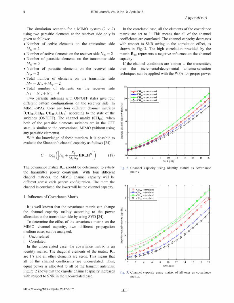
The simulation scenario for a MIMO system (2 9 2)using two parasitic elements at the receiver side only isgiven as follows:
• Number of active elements on the transmitter sideM ta ¼ 2
• Number of active elements on the receiver side N ra ¼ 2
• Number of parasitic elements on the transmitter sideM tp ¼ 0
• Number of parasitic elements on the receiver sideN rp ¼ 2
• Total number of elements on the transmitter sideMT ¼ M ta þM tp ¼ 2
• Total number of elements on the receiver sideNR ¼ N ra þ N rp ¼ 4Two parasitic antennas with ON/OFF states give four
different pattern configurations on the receiver side. InMIMO-SPAs, there are four different channel matricesCH00;CH01;CH10;CH11ð Þ; according to the state of theswitches (ON/OFF). The channel matrix (CH00), whenboth of the parasitic elements switches are in the OFFstate, is similar to the conventional MIMO (without usingany parasitic elements).With the knowledge of these matrices, it is possible to
evaluate the Shannon’s channel capacity as follows [24]:
C ¼ log2 INR þES
MTN0HRssHH
: (18)
The covariance matrix Rss should be determined to satisfythe transmitter power constraints. With four differentchannel matrices, the MIMO channel capacity will bedifferent across each pattern configuration. The more thechannel is correlated, the lower will be the channel capacity.
1. Influence of Covariance Matrix
It is well known that the covariance matrix can changethe channel capacity mainly according to the powerallocation at the transmitter side by using SVD [24].To determine the effect of the covariance matrix on the
MIMO channel capacity, two different propagationmedium cases can be analyzed:i Uncorrelatedii Correlated.In the uncorrelated case, the covariance matrix is an
identity matrix. The diagonal elements of the matrix Rss
are 1’s and all other elements are zeros. This means thatall of the channel coefficients are uncorrelated. Thus,equal power is allocated to all of the transmit antennas.Figure 2 shows that the ergodic channel capacity increaseswith respect to SNR in the uncorrelated case.
In the correlated case, all the elements of the covariancematrix are set to 1. This means that all of the channelcoefficients are correlated. The channel capacity decreaseswith respect to SNR owing to the correlation effect, asshown in Fig. 3. The high correlation provided by thematrix Rss, represents a negative influence on the channelcapacity.If the channel conditions are known to the transmitter,
then the incremental/decremental antenna-selectiontechniques can be applied with the WPA for proper power
00
SNR (dB)
Ergo
dic
chan
nel c
apac
ity (b
ps/H
z)
2
4
6
8
10
12
2 4 6 8 10 12 14 16 18 20
CH00 uncorrelatedCH01 uncorrelatedCH10 uncorrelatedCH11 uncorrelated
Fig. 2. Channel capacity using identity matrix as covariancematrix.
00
SNR (dB)
Ergo
dic
chan
nel c
apac
ity (b
ps/H
z)
1
2
3
4
5
6
2 4 6 8 10 12 14 16 18 20
CH00 correlatedCH01 correlatedCH10 correlated CH11 correlated
Fig. 3. Channel capacity using matrix of all ones as covariancematrix.
6 ETRI Journal, Vol. 0, No. 0, April 2018
https://doi.org/10.4218/etrij.2017-0071
Appendix-A
165

allocation at the transmitter side. The knowledge of thechannel conditions can be fed back to the transmitter inthe form of a covariance matrix. The covariance matrix
represents the correlation present in the channel, and withWPA, more power can be distributed to the best channel,and less power to channels that contribute less to thechannel capacity.A comparison of four different configurations for the
uncorrelated case with and without WPA is shown inFig. 4. For all of the parasitic configurations, the MIMOchannel capacity is improved with the power allocationusing WPA as compared to the equal power distributionacross all the eigenvalues.
2. Comparison of Different Covariance Matrices
In this section, the I-AST is used to select the best set ofantennas, and then allocates power by carrying out WPA.The comparison between covariance matrices across all
the pattern configurations is shown in Fig. 5. Thecomparison is discussed with three different covariancematrices as follows:
• I-AST with correlated covariance matrix- Rss½ corr• I-AST with uncorrelated covariance matrix- Rss½ uncorr• I-AST with improved covariance matrix WPA- Rss½ WPA
00
SNR (dB)
Ergo
dic
chan
nel c
apac
ity (b
ps/H
z)
2
4
6
8
10
12
2 4 6 8 10 12 14 16 18 20
CH00 WPACH00 w/o WPACH01 WPACH01 w/o WPACH10 WPACH10 w/o WPACH11 WPACH11 w/o WPA
Fig. 4. Comparison of all pattern configuration matrices withand without WPA.
Cha
nnel
cap
acity
(bps
/Hz)
00
2
4
6
8
10
12
2 4 6 8 10 12 14 16 18 20SNR (dB)
CH00 WPACH00 uncorrelatedCH00 correlated
Cha
nnel
cap
acity
(bps
/Hz)
00
2
4
6
8
10
12
2 4 6 8 10 12 14 16 18 20SNR (dB)
Cha
nnel
cap
acity
(bps
/Hz)
00
2
4
6
8
10
12
2 4 6 8 10 12 14 16 18 20SNR (dB)
Cha
nnel
cap
acity
(bps
/Hz)
00
2
4
6
8
10
12
2 4 6 8 10 12 14 16 18 20SNR (dB)
CH10 WPACH10 uncorrelatedCH10 correlated
CH11 WPACH11 uncorrelatedCH11 correlated
CH01 WPACH01 uncorrelatedCH01 correlated
Fig. 5. Comparison of channel capacity with three different forms of covariance matrices across all pattern configurations.
7Paramvir Kaur Pal and Robert Simon Sherratt
http://onlinelibrary.wiley.com/journal/10.4218/(ISSN)2233-7326
Appendix-A
166

In this comparison, when the channel matrix iscorrelated, it gives the lower bounds for the MIMOchannel capacity for all of the pattern configurations.When the channel matrix is uncorrelated with I-AST, thechannel capacity is improved compared to the correlatedcase. Figure 5 shows that when the covariance matrix isimproved with WPA, in all different configurationmatrices, the channel capacity provides the upper bounds.These are the bounds according to the influence of thecovariance matrix in three different cases.
3. Pattern Configuration Selection
CN is known as the channel quality indicator and usedto obtain the best pattern configuration. It represents theEVS of the channel as [15]:
CN ¼ kmax
kmin; (19)
where kmax and kmin are the maximum and minimumeigenvalues of the covariance matrix, respectively.If eigenvalues of the covariance matrix are less spread
out, it provides a small CN value. In MIMO-SPAs, thereare four different pattern configurations. All four patternconfigurations represent the four different channelmatrices CH00;CH01;CH10;CH11ð Þ, and have differentCNs. By performing the exhaustive search, the channelmatrix or pattern that has a low CN is selected. For theselection purpose in the uncorrelated case, as shown inFig. 5, the pattern configuration CH10 matrix with thelowest CN is selected. This is the optimal patternconfiguration with the best channel quality, and provides
the greatest channel capacity compared with otherconfigurations.
4. Pattern Configuration for Different SNR Values
The MIMO channel capacity also depends on the SNRvalues. The behavior of four pattern configurations atdifferent SNRs levels are shown in Fig. 6. It can be seenthat at 5 dB–15 dB, the second pattern configurationCH01 provides the highest channel capacity.At 20 dB and 25 dB, the third configuration CH10 can
be selected as it provides the highest channel capacity.
V. Conclusion
SPAs offer a significant advantage in terms of the use ofhandheld devices, where space, cost, and hardwarecomplexity are the primary constraints. The mainadvantages of SPAs are their ability to change theirradiation pattern and to operate within a specific changingenvironment, while maintaining good electromagneticcharacteristics. For simplicity, and to provide a limitedlevel of pattern diversity, only two switch positions (ON/OFF) were used in this study.Based on the knowledge of the channel statistics, a
decomposition model decouples the transmit signal intoorthogonal eigenbeams. The power distribution assignedto these eigenvalues is according to the WPA, whichmeans that there is a greater power in directions where thechannel is strong, but reduced or no power in directionswith weak channels. Using the I-AST technique withWPA, the MIMO-SPAs channel capacity is significantlyimproved for all the pattern configurations. A comparisonof three covariance matrices showed that the improvedpower allocation of the covariance matrix with WPA has ahigher channel capacity than others.The novel contribution of this paper is the use of the CN
as a selection criterion to determine the optimal patternconfiguration for the receiver antenna array. The behavior ofthe CN of the covariance matrix represents the EVS of thechannel. Using a good-quality channel, a high multiplexinggain can be achieved with proper transmission. Thus, theCN is an excellent indicator of channel quality, and is a veryuseful metric in link adaptation schemes.In the future, this work will be extended for application
to multicarrier systems such as orthogonal frequency-division multiplexing (OFDM), where it is possible toselect the pattern selection using the CN across a numberof subcarriers. It also has the advantage of feedback andbandwidth reduction in future wireless communicationsystems.
5
CH00
Ergo
dic
chan
nel c
apac
ity (b
ps/H
z)
Parasitic array configurations
10
15
20
25
30
35
40
CH01 CH10 CH11
SNR = 5 dBSNR = 10 dBSNR = 15 dBSNR = 20 dBSNR = 25 dB
Fig. 6. Pattern configuration selection at different SNR values.
8 ETRI Journal, Vol. 0, No. 0, April 2018
https://doi.org/10.4218/etrij.2017-0071
Appendix-A
167

References
[1] E. Telatar, “Capacity of Multi-antenna Gaussian Channel,”
Trans. Emerg. Telecommun. Technol., vol. 10, no. 6, Nov.1999, pp. 585–595.
[2] G.J. Foschini and M.J. Gans, “On Limits of WirelessCommunications in a Fading Environment when Using
Multiple Antennas,” Wireless Personal Commun., vol. 6,no. 3, Mar. 1998, pp. 311–335.
[3] R. Vaughan, “Switched Parasitic Elements for AntennaDiversity,” IEEE Trans. Antennas Propag., vol. 47, no. 2,Feb. 1999, pp. 399–405.
[4] M. Wennstrom and T. Svantesson, “An Antenna Solutionfor MIMO Channels: The Switched Parasitic Antenna,”
IEEE Int. Symp. Personal, Indoor Mobile Radio Commun.,San Diego, CA, USA, Sept. 2001, pp. 159–163.
[5] A. Kalis, A.G. Kanatas, and C.B. Papadias, “A NovelApproach to MIMO Transmission Using a Single RF Front
End,” IEEE J. Sel. Areas Commun., vol. 26, no. 6, Aug.2008, pp. 972–980.
[6] A. Kalis, A.G. Kanatas, and C.B. Papadias, Parasitic
Antenna Arrays for Wireless MIMO Systems, New York,USA: Springer, 2014.
[7] M.D. Migliore, D. Pinchera, and F. Schettino, “ImprovingChannel Capacity Using Adaptive MIMO Antennas,” IEEE
Trans. Antennas Propag., vol. 54, no. 11, Nov. 2006, pp.3481–3489.
[8] O.N. Alrabadi, C. Divarathne, P. Tragas, A. Kalis, N.Marchetti, C.B. Papadias, and R. Prasad, “Spatial
Multiplexing with a Single Radio: Proof-of-ConceptExperiments in an Indoor Environment with a 2.6 GHzPrototype,” IEEE Commun. Lett., vol. 15, no. 2, Feb. 2011,
pp. 178–180.[9] O.N. Alrabadi, J. Perruisseau-Carrier, and A. Kalis,
“MIMO Transmission Using a Single RF Source: Theoryand Antenna Design,” IEEE Trans. Antennas Propag., vol.
60, no. 2, Feb. 2012, pp. 654–664.[10] D. Gwak, I. Sohn, and S.H. Lee, “Analysis of Single-RF
MIMO Receiver with Beam-Switching Antenna,” ETRI J.,vol. 37, no. 4, Aug. 2015, pp. 647–656.
[11] R. Bains and R. Muller, “Using Parasitic Elements for
Implementing the Rotating Antenna for MIMO Receivers,”IEEE Trans. Wireless Commun., vol. 7, no. 11, Nov. 2008,
pp. 4522–4533.[12] M. DiZazzo, M.D. Migliore, F. Schettino, V. Patriarca, and
D. Pinchera, “A Novel Parasitic-MIMO Antenna,” IEEE
Antennas Propag. Soc. Inter. Symp., Albuquerque, NM,
USA, July 2006, pp. 4447–4450.[13] M. Yoshida, K. Sakaguchi, and K. Araki, “Single Front-
End MIMO Architecture with Parasitic Antenna Elements,”
IEICE Trans. Commun., vol. E95-B, no. 3, Mar. 2012, pp.882–888.
[14] M. Vu and A. Paulraj, “MIMO Wireless Linear Precoding,”
IEEE Signal Process. Mag., vol. 24, no. 5, Sept. 2007, pp.86–105.
[15] D. Sacristan-Murga and A. Pascual-Iserte, “DifferentialFeedback of MIMO Channel Gram Matrices Based on
Geodesic Curves,” IEEE Trans. Wireless Commun., vol. 9,no. 12, Dec. 2010, pp. 3714–3727.
[16] D. Tse and P. Viswanath, Fundamentals of Wireless
Communication, Cambridge, UK: Cambridge UniversityPress, 2005.
[17] J. Zik, Maximizing LTE Performance through MIMO
Optimization, Germantown, PA, USA: PCTEL Inc., Apr.
2011.[18] M. Zia, T. Kiani, H. Mahmood, T. Shah, and N.A. Saqib,
“Bandwidth-Efficient Selective Retransmission for MIMO-OFDM Systems,” ETRI J., vol. 37, no. 1, Feb. 2015, pp.
66–76.[19] R.W. Heath and A.J. Paulraj, “Switching Between Diversity
and Multiplexing in MIMO Systems,” IEEE Trans.
Commun., vol. 53, no. 6, 2005, pp. 962–968.[20] D. Piazza, J. Kountouriotis, M. D’Amico, and K.R.
Dandekar, “A Technique for Antenna ConfigurationSelection for Reconfigurable Circular Patch Arrays,” IEEE
Trans. Antennas Propag., vol. 8, no. 3, Mar. 2009, pp.1456–1467.
[21] A. Forenza, A. Pandharipande, H. Kim, and R.W. Heath,“Adaptive MIMO Transmission Scheme: Exploiting the
Spatial Selectivity of Wireless Channels,” IEEE Veh.
Technol. Conf., Stockholm, Sweden, May 30–June 1, 2005,pp. 3188–3192.
[22] D. Pinchera and M.D. Migliore, “Effectively ExploitingParasitic Arrays for Secret Key Sharing,” IEEE Trans. Veh.
Tech., vol. 65, no. 1, Jan. 2016, pp. 123–131.[23] R.W. Heath and D.J. Love, “Multimode Antenna Selection
for Spatial Multiplexing Systems with Linear Receivers,”IEEE Trans. Signal Process., vol. 53, no. 8, Aug. 2005, pp.
3042–3056.[24] J.V. Cuan-Cortes, C. Vargas-Rosales, and D. Munoz-
Rodriguez, “MIMO Channel Capacity Using AntennaSelection and Water Pouring,” EURASIP J. Wireless
Commun. Netw., vol. 2014, Dec. 2014, pp. 1–10.
[25] C.A. Balanis, Antenna Theory, New York, USA: Wiley,2005.
[26] C.E. Shannon, “A Mathematical Theory of Communication,”Bell Syst. Tech. J., vol. 27, no. 3, 1948, pp. 379–423.
[27] S.J. Orfanidis, “Electromagnetic Waves and Antennas,”Rutgers University, 2002, pp. 702–733, Accessed 2017.
http://www.ece.rutgers.edu/~orfanidi/ewa/
9Paramvir Kaur Pal and Robert Simon Sherratt
http://onlinelibrary.wiley.com/journal/10.4218/(ISSN)2233-7326
Appendix-A
168

[28] M.R.O. Mofolo, A.A. Lysko, T.O. Olwal, and W.A. Clarke,“Beam Steering for Circular Switched Parasitic ArraysUsing a Combinational Approach,” IEEE AFRICON,
Livingstone, Zambia, Sept. 13–15, 2011, pp. 1–6.[29] K. Gyoda and T. Ohira, “Design of Electronically Steerable
Passive Array Radiator (ESPAR) Antennas,” IEEE
Antennas Propag. Soc. Int. Symp., Salt Lake City, UT,
USA, July 16–21, 2000, pp. 922–925.
Paramvir Kaur Pal received her BEngdegree in electronics engineering from
Nagpur University, India, in 2001, and herMEng degree in electronics from Punjab
Engineering College, Chandigarh, India in2004. From 2004 to 2006, she worked as a
lecturer at the Shaheed Udham SinghCollege of Engineering and Technology, Mohali, India. She iscurrently pursuing her PhD degree at the University of Reading,
UK. Her research interests are in the area of MIMO wirelesscommunication for closely spaced antennas and spatial
multiplexing.
Robert Simon Sherratt received hisBEng degree in electronic systems and
control engineering from Sheffield CityPolytechnic, UK, in 1992, and his MSc
and PhD degrees in electronic engineeringfrom the University of Salford, UK, in
1994 and 1996, respectively. From 1996,he has been with the University of Reading, UK, where he isnow a full professor. His research areas are signal processing and
personal communications in consumer devices, focusing onwearable devices for healthcare applications.
10 ETRI Journal, Vol. 0, No. 0, April 2018
https://doi.org/10.4218/etrij.2017-0071
Appendix-A
169
MATLAB Code
clear all;
clc;
%Antenna Specifications to generate radiation patterns
N=4; % Active Element=2 + Parasitic Element=2 --- at Rx side
M=2; % Active Element=2 + Parasitic Element=0--- at Tx side
c=3e8; %speed of light in m/s
f=2.4e9; %operational frequency
lambda=(c/f); %lambda=c/f
phi=((0:2*pi/359:2*pi));
L = [0.5, 0.5,0.5,0.5]; % lengths of the antenna elements
a = [0.001, 0.001,0.001,0.001]; % radii of the antenna elements
d = [0.125,0; -0.125,0; 0,0.125;0,-0.125]; % xy locations
%%%%%%%%%%%%%%%%%%%%%%%%%%%%%%%%%%%%%%%%%%%
V=[1 1 0 0]'; %Driving voltages
Z = impedmat(L,a,d); % impedance matrix
%Combinations of the parasitic load values
Zload1 = [50 0 0 0;
0 50 0 0;
0 0 10000 0;
0 0 0 10000];
Zload2 = [50 0 0 0;
0 50 0 0;
0 0 10000 0;
0 0 0 1];
Zload3 = [50 0 0 0;
0 50 0 0;
0 0 1 0;
0 0 0 10000];
Zload4 = [50 0 0 0;
0 50 0 0;
0 0 1 0;
0 0 0 1];
% Calculate impedance matrix with parasitic load values
Z_r=Z;
Z_Rx1=Z_r+Zload1;
Appendix-B
170

Inv_Z_Rx1=inv(Z_Rx1);
Z_Rx11=Z_r*(Inv_Z_Rx1);
I1=Z_Rx1\V;
[ge1,gh1,gt1]=gain2(L,d,I1,359);
Z_Rx2=Z_r+Zload2;
Inv_Z_Rx2=inv(Z_Rx2);
Z_Rx22=Z_r*(Inv_Z_Rx2);
I2=Z_Rx2\V;
[ge2,gh2,gt2]=gain2(L,d,I2,359);
Z_Rx3=Z_r+Zload3;
Inv_Z_Rx3=inv(Z_Rx3);
Z_Rx33=Z_r*(Inv_Z_Rx3);
I3=Z_Rx3\V;
[ge3,gh3,gt3]=gain2(L,d,I3,359);
Z_Rx4=Z_r+Zload4;
Inv_Z_Rx4=inv(Z_Rx4);
Z_Rx44=Z_r*(Inv_Z_Rx4);
I4=Z_Rx4\V;
[ge4,gh4,gt4]=gain2(L,d,I4,359);
Z_Tx1=Z_Rx1;
Z_Tx2=Z_Rx2;
Z_Tx3=Z_Rx3;
Z_Tx4=Z_Rx4;
MaxIter=100; % Maximum Iterations
SNRdBs=[0:20];
for i=1:length(SNRdBs)
SNRdB = SNRdBs(i);
cum00_corr=0;
cum00_uncorr=0;
cum00_WPA=0;
cum01_corr=0;
cum01_uncorr=0;
cum01_WPA=0;
cum10_corr=0;
cum10_uncorr=0;
cum10_WPA=0;
cum11_corr=0;
cum11_uncorr=0;
cum11_WPA=0;
cumAE=0;
Appendix-B
171

for n=1:MaxIter
rand('seed',1);
randn('seed',1);
G=sqrt(0.5)*(randn(N,M)+1j*randn(N,M));
H_hat1=Z_Rx11*G*eye(2);
H_hat2=Z_Rx22*G*eye(2);
H_hat3=Z_Rx33*G*eye(2);
H_hat4=Z_Rx44*G*eye(2);
S_r=zeros(2,4);
S_t=zeros(4,2);
S_r(1,1)=1;
S_r(2,2)=1;
S_t=eye(2);
H1=S_r*H_hat1*S_t;
H2=S_r*H_hat2*S_t;
H3=S_r*H_hat3*S_t;
H4=S_r*H_hat4*S_t;
I=eye(2,2);
I_corr=ones(2,2);
%%%%%%%%%%%%%%%%%%%%%%%%%%%%%%%%%%%%%%%%%%%%
%H00-H1--2X2%%%%%%%%%%%%%%%%%%%%%%%%%%%%%%%%%%%%
H00_1=H1(:,1);
H00_2=H1(:,2);
sel_ant1=1;
SNR_sel_ant1 = 10.^(SNRdB/10)/sel_ant1;
log_SH00_1 = log2(real(det(I+SNR_sel_ant1*H00_1*H00_1')));
log_SH00_2 = log2(real(det(I+SNR_sel_ant1*H00_2*H00_2')));
log_SH00=[log_SH00_1 log_SH00_2 ];
c00=sort(log_SH00,'descend');
node00_1=find(c00(1)==log_SH00);
node00_2=find(c00(2)==log_SH00);
node00=[node00_1 node00_2 ];
newH00_1=H1(:,node00_1);
newH00_2=H1(:,node00_2);
%%%%%%%%%%%%%%%%%%%%%%%%%%%%%%%%%%%%%%%%%%%%
Appendix-B
172

newH00=[newH00_1 newH00_2];
SV00 = svd(newH00'*newH00);
Gamma00 = Water_Pouring(SV00,SNR_sel_ant1,2);
maximum_capacity00_WPA = log2(det(I+SNR_sel_ant1/2*diag(Gamma00)*diag(SV00)));
maximum_capacity_00_uncorr = log2(real(det(I+SNR_sel_ant1/2*H1'*H1)));
maximum_capacity_00_corr = log2(real(det(I+SNR_sel_ant1/2*I_corr*H1'*H1)));
%%%%%%%%%%%%%%%%%%%%%%%%%%%%%%%%%%%%%%%%%%%%%
cum00_uncorr = cum00_uncorr + maximum_capacity_00_uncorr; % uncorrelated
cum00_WPA = cum00_WPA + maximum_capacity00_WPA; % WPA
cum00_corr=cum00_corr + maximum_capacity_00_corr; % correlated
%%%%%%%%%%%%%%%%%%%%%%%%%%%%%%%%%%%%%%%%%%%%%
%H01----H2---2X2%%%%%%%%%%%%%%%%%%%%%%%%%%%%%%%%%%%%
H01_1=H2(:,1);
H01_2=H2(:,2);
sel_ant1=1;
SNR_sel_ant1 = 10.^(SNRdB/10)/sel_ant1;
log_SH01_1 = log2(real(det(I+SNR_sel_ant1*H01_1*H01_1')));
log_SH01_2 = log2(real(det(I+SNR_sel_ant1*H01_2*H01_2')));
log_SH01=[log_SH01_1 log_SH01_2 ];
c01=sort(log_SH01,'descend');
node01_1=find(c01(1)==log_SH01);
node01_2=find(c01(2)==log_SH01);
node01=[node01_1 node01_2];
newH01_1=H2(:,node01_1);
newH01_2=H2(:,node01_2);
%%%%%%%%%%%%%%%%%%%%%%%%%%%%%%%%%%%%%%%%%%%%%
newH01=[newH01_1 newH01_2];
SV01 = svd(newH01'*newH01);
Gamma01 = Water_Pouring(SV01,SNR_sel_ant1,2);
maximum_capacity01_WPA = log2(det(I+SNR_sel_ant1/2*diag(Gamma01)*diag(SV01)));
maximum_capacity_01_uncorr = log2(real(det(I+SNR_sel_ant1/2*H2'*H2)));
maximum_capacity_01_corr = log2(real(det(I+SNR_sel_ant1/2*I_corr*H2'*H2)));
%%%%%%%%%%%%%%%%%%%%%%%%%%%%%%%%%%%%%%%%%%%%%
cum01_uncorr = cum01_uncorr + maximum_capacity_01_uncorr; % uncorrelated
cum01_WPA = cum01_WPA + maximum_capacity01_WPA; % WPA
cum01_corr=cum01_corr + maximum_capacity_01_corr; % correlated
Appendix-B
173

%%%%%%%%%%%%%%%%%%%%%%%%%%%%%%%%%%%%%%%%%%%%
%%H10----H3---2X2%%%%%%%%%%%%%%%%%%%%%%%%%%%%%%%%%
H10_1=H3(:,1);
H10_2=H3(:,2);
sel_ant1=1;
SNR_sel_ant1 = 10.^(SNRdB/10)/sel_ant1;
log_SH10_1 = log2(real(det(I+SNR_sel_ant1*H10_1*H10_1')));
log_SH10_2 = log2(real(det(I+SNR_sel_ant1*H10_2*H10_2')));
log_SH10=[log_SH10_1 log_SH10_2 ];
c10=sort(log_SH10,'descend');
node10_1=find(c10(1)==log_SH10);
node10_2=find(c10(2)==log_SH10);
node10=[node10_1 node10_2];
newH10_1=H3(:,node10_1);
newH10_2=H3(:,node10_2);
%%%%%%%%%%%%%%%%%%%%%%%%%%%%%%%%%%%%%%%%%%%
newH10=[newH10_1 newH10_2 ];
SV10 = svd(newH10'*newH10);
Gamma10 = Water_Pouring(SV10,SNR_sel_ant1,2);
maximum_capacity10_WPA = log2(det(I+SNR_sel_ant1/2*diag(Gamma10)*diag(SV10)));
maximum_capacity_10_uncorr = log2(real(det(I+SNR_sel_ant1/2*H3'*H3)));
maximum_capacity_10_corr = log2(real(det(I+SNR_sel_ant1/2*I_corr*H3'*H3)));
%%%%%%%%%%%%%%%%%%%%%%%%%%%%%%%%%%%%%%%%%%
cum10_uncorr = cum10_uncorr + maximum_capacity_10_uncorr; % uncorrelated
cum10_WPA = cum10_WPA + maximum_capacity10_WPA; % WPA
cum10_corr=cum10_corr + maximum_capacity_10_corr; % correlated
%%%%%%%%%%%%%%%%%%%%%%%%%%%%%%%%%%%%%%%%%%%
%H11----H4---2X2%%%%%%%%%%%%%%%%%%%%%%%%%%%%%%%%%%
H11_1=H4(:,1);
H11_2=H4(:,2);
sel_ant1=1;
SNR_sel_ant1 = 10.^(SNRdB/10)/sel_ant1;
log_SH11_1 = log2(real(det(I+SNR_sel_ant1*H11_1*H11_1')));
log_SH11_2 = log2(real(det(I+SNR_sel_ant1*H11_2*H11_2')));
log_SH11=[log_SH11_1 log_SH11_2 ];
Appendix-B
174

c11=sort(log_SH11,'descend');
node11_1=find(c11(1)==log_SH11);
node11_2=find(c11(2)==log_SH11);
node11=[node11_1 node11_2];
newH11_1=H4(:,node11_1);
newH11_2=H4(:,node11_2);
%%%%%%%%%%%%%%%%%%%%%%%%%%%%%%%%%%%%%%%%%%
newH11=[newH11_1 newH11_2 ];
SV11 = svd(newH11'*newH11);
Gamma11 = Water_Pouring(SV11,SNR_sel_ant1,2);
maximum_capacity11_WPA = log2(det(I+SNR_sel_ant1/2*diag(Gamma11)*diag(SV11)));
maximum_capacity_11_uncorr = log2(real(det(I+SNR_sel_ant1/2*H4'*H4)));
maximum_capacity_11_corr = log2(real(det(I+SNR_sel_ant1/2*I_corr*H4'*H4)));
%%%%%%%%%%%%%%%%%%%%%%%%%%%%%%%%%%%%%%%%%%
cum11_uncorr = cum11_uncorr + maximum_capacity_11_uncorr; % uncorrelated
cum11_WPA = cum11_WPA + maximum_capacity11_WPA; % WPA
cum11_corr=cum11_corr + maximum_capacity_11_corr; % correlated
%%%%%%%%%%%%%%%%%%%%%%%%%%%%%%%%%%%%%%%%%%
%Without Parasitic elements---only Active Elements
%Impedance Matrix with only Active Elements
L1 = [0.5, 0.5]; % lengths
a1 = [0.001, 0.001]; % radii
d1 = [0.125,0; -0.125,0]; % xy locations
phi1=((0:2*pi/359:2*pi));
V1=[1 1]'; %Driving voltages
Z1 = impedmat(L1,a1,d1); % impedance matrix
Z_AE=Z1;
Zload_AE = [50 0;
0 50];
Z_Rx_AE=Z_AE+Zload_AE;
Inv_Z_Rx_AE=inv(Z_Rx_AE);
Z_Rx_AAEE=Z_AE*(Inv_Z_Rx_AE);
I_AE=Z_Rx_AE\V1;
[ge5,gh5,gt5]=gain2(L1,d1,I_AE,359);
%%%%%%%%%%%%%%%%%%%%%%%%%%%%%%%%%%%%%%%%%%%
H_AE=G(1:2,1:2);
H_hat_AE=Z_Rx_AAEE*H_AE*eye(2);
Appendix-B
175

cumAE=cumAE+log2(real(det(I+(SNR_sel_ant1/2)*H_hat_AE'*H_hat_AE)));
end
%%%%%%%%%%%%%%%%%%%%%%%%%%%%%%%%%%%%%%%%%%%%
sel_capacity00_uncorr(i) = cum00_uncorr/MaxIter;
sel_capacity00_corr(i) = cum00_corr/MaxIter;
sel_capacity00_WPA(i) = cum00_WPA/MaxIter;
sel_capacity01_uncorr(i) = cum01_uncorr/MaxIter;
sel_capacity01_corr(i) = cum01_corr/MaxIter;
sel_capacity01_WPA(i) = cum01_WPA/MaxIter;
sel_capacity10_uncorr(i) = cum10_uncorr/MaxIter;
sel_capacity10_corr(i) = cum10_corr/MaxIter;
sel_capacity10_WPA(i) = cum10_WPA/MaxIter;
sel_capacity11_uncorr(i) = cum11_uncorr/MaxIter;
sel_capacity11_corr(i) = cum11_corr/MaxIter;
sel_capacity11_WPA(i) = cum11_WPA/MaxIter;
sel_capacityAE(i) = cumAE/MaxIter;
end
sel_capacity = [sel_capacity00_uncorr' sel_capacity01_uncorr' sel_capacity10_uncorr'
sel_capacity11_uncorr'];
sel_capacity_AS = [sel_capacity00_WPA' sel_capacity01_WPA' sel_capacity10_WPA'
sel_capacity11_WPA'];
%%%%%%%%%%%%%%%%%%%%%%%%%%%%%%%%%%%%%%%%%%%
%Condition Number (CN)
CN1=cond(H1);
CN2=cond(H2);
CN3=cond(H3);
CN4=cond(H4);
CN=[CN1 CN2 CN3 CN4];
%Optimal CN
CN_lowest=sort(CN,'ascend');
BEST=find(CN_lowest(1)==CN);
%Condition Number (CN) in dB
CN_dB1=20.*log10(CN1);
CN_dB2=20.*log10(CN2);
CN_dB3=20.*log10(CN3);
CN_dB4=20.*log10(CN4);
CN_dB=[CN_dB1 CN_dB2 CN_dB3 CN_dB4];
Appendix-B
176

CN_dB_lowest=sort(CN_dB,'ascend');
BEST_dB=find(CN_dB_lowest(1)==CN_dB)
%%%%%%%%%%%%%%%%%%%%%%%%%%%%%%%%%%%%%%%%%%%%%
figure(1);
plot(SNRdBs,sel_capacity00_WPA,'-ro',SNRdBs,sel_capacity00_uncorr,'--ro',
SNRdBs, sel_capacity00_corr,':ro',SNRdBs,sel_capacity01_WPA,'-bx',
SNRdBs,sel_capacity01_uncorr,'--bx',SNRdBs,sel_capacity01_corr,':bx',
SNRdBs,sel_capacity10_WPA,'-gs',SNRdBs,sel_capacity10_uncorr,'--gs',
SNRdBs,sel_capacity10_corr,':gs',SNRdBs,sel_capacity11_WPA,'-kd',
SNRdBs,sel_capacity11_uncorr,'--kd',SNRdBs,sel_capacity11_corr,':kd');
xlabel('SNR [dB]');
ylabel('Ergodic Channel Capacity (bps/Hz)');
set(0,'DefaultAxesFontName', 'Times New Roman');
set(0,'DefaultAxesFontSize', 10);
grid on;
legend('CH00 WPA','CH00 Uncorrelated','CH00 Correlated',...
'CH01 WPA','CH01 Uncorrelated','CH01 Correlated',...
'CH10 WPA','CH10 Uncorrelated','CH10 Correlated',...
'CH11 WPA','CH11 Uncorrelated','CH11 Correlated');
legend('Location','Northwest');
%%%%%%%%%%%%%%%%%%%%%%%%%%%%%%%%%%%%%%%%%%%%%%
figure(2);
plot(SNRdBs,sel_capacity00_WPA,'-ko',SNRdBs,sel_capacity00_uncorr,'--ko',
SNRdBs, sel_capacity00_corr,':ko',SNRdBs,sel_capacity01_WPA,'-kx',
SNRdBs,sel_capacity01_uncorr,'--kx', SNRdBs,sel_capacity01_corr,':kx',
SNRdBs,sel_capacity10_WPA,'-ks',SNRdBs,sel_capacity10_uncorr,'--ks',
SNRdBs,sel_capacity10_corr,':ks',SNRdBs,sel_capacity11_WPA,'-kd',
SNRdBs,sel_capacity11_uncorr,'--kd',SNRdBs,sel_capacity11_corr,':kd');
xlabel('SNR [dB]');
ylabel('Ergodic Channel Capacity (bps/Hz)');
set(0,'DefaultAxesFontName', 'Times New Roman');
set(0,'DefaultAxesFontSize', 10);
grid on;
legend('CH00 WPA','CH00 Uncorrelated','CH00 Correlated',...
'CH01 WPA','CH01 Uncorrelated','CH01 Correlated',...
'CH10 WPA','CH10 Uncorrelated','CH10 Correlated',...
Appendix-B
177

'CH11 WPA','CH11 Uncorrelated','CH11 Correlated');
legend('Location','Northwest');
%%%%%%%%%%%%%%%%%%%%%%%%%%%%%%%%%%%%%%%%%%%%%%%
figure(3);
h = subplot(2,2,1)
plot( SNRdBs,sel_capacity00_WPA,'-k*',SNRdBs,sel_capacity00_uncorr,'-ko',
SNRdBs,sel_capacity00_corr,'-kd');
xlabel('SNR[dB]');
ylabel('Channel Capacity (bps/Hz)');
set(0,'DefaultAxesFontName', 'Times New Roman')
set(0,'DefaultAxesFontSize', 8)
grid on;
legend('CH00 WPA','CH00 Uncorrelated','CH00 Correlated');
legend('Location','Northwest');
xlim([0 20]);
ylim([0 12]);
h = subplot(2,2,2);
plot(SNRdBs,sel_capacity01_WPA,'-k*',SNRdBs,sel_capacity01_uncorr,'-ko',
SNRdBs,sel_capacity01_corr,'-kd')
xlabel('SNR[dB]');
ylabel('Channel Capacity (bps/Hz)');
set(0,'DefaultAxesFontName', 'Times New Roman');
set(0,'DefaultAxesFontSize', 8);
grid on;
legend('CH01 WPA','CH01 Uncorrelated','CH01 Correlated');
legend('Location','Northwest');
xlim([0 20]);
ylim([0 12]);
h = subplot(2,2,3);
plot( SNRdBs,sel_capacity10_WPA,'-k*',SNRdBs,sel_capacity10_uncorr,'-ko',
SNRdBs,sel_capacity10_corr,'-kd')
xlabel('SNR[dB]');
ylabel('Channel Capacity (bps/Hz)');
set(0,'DefaultAxesFontName', 'Times New Roman');
set(0,'DefaultAxesFontSize', 8);
grid on;
legend('CH10 WPA','CH10 Uncorrelated','CH10 Correlated');
legend('Location','Northwest');
xlim([0 20]);
ylim([0 12]);
h = subplot(2,2,4);
plot(SNRdBs,sel_capacity11_WPA,'-k*',SNRdBs,sel_capacity11_uncorr,'-ko',
Appendix-B
178

SNRdBs,sel_capacity11_corr,'-kd')
xlabel('SNR[dB]');
ylabel('Channel Capacity (bps/Hz)');
set(0,'DefaultAxesFontName', 'Times New Roman');
set(0,'DefaultAxesFontSize', 8);
grid on;
legend('CH11 WPA','CH11 Uncorrelated','CH11 Correlated');
legend('Location','Northwest');
xlim([0 20]);
ylim([0 12]);
subplotsqueeze(gcf, 1.2);
%%%%%%%%%%%%%%%%%%%%%%%%%%%%%%%%%%%%%%%%%%%%%%
figure(4);
plot(SNRdBs,sel_capacity00_uncorr,'-ro',SNRdBs,sel_capacity01_uncorr,'--bx',
SNRdBs,sel_capacity10_uncorr,'--gs',SNRdBs,sel_capacity11_uncorr,'--kd')
xlabel('SNR [dB]');
ylabel('Ergodic Channel Capacity (bps/Hz)');
set(0,'DefaultAxesFontName', 'Times New Roman');
set(0,'DefaultAxesFontSize', 10);
grid on;
legend('CH00','CH01','CH10','CH11');
legend('Location','Northwest');
%%%%%%%%%%%%%%%%%%%%%%%%%%%%%%%%%%%%%%%%%%%%%%%
figure(5);
plot(SNRdBs,sel_capacity00_uncorr,'-ko',SNRdBs,sel_capacity01_uncorr,'-kx',
SNRdBs,sel_capacity10_uncorr,'-ks',SNRdBs,sel_capacity11_uncorr,'-kd')
xlabel('SNR [dB]');
ylabel('Ergodic Channel Capacity (bps/Hz)');
set(0,'DefaultAxesFontName', 'Times New Roman');
set(0,'DefaultAxesFontSize', 10);
grid on;
legend('CH00 Uncorrelated','CH01 Uncorrelated','CH10 Uncorrelated','CH11 Uncorrelated');
legend('Location','Northwest');
%%%%%%%%%%%%%%%%%%%%%%%%%%%%%%%%%%%%%%%%%%%%%%
figure(6);
plot(SNRdBs, sel_capacity00_corr,':ro',SNRdBs,sel_capacity01_corr,':bx',
SNRdBs,sel_capacity10_corr,':gs',SNRdBs,sel_capacity11_corr,':kd')
xlabel('SNR [dB]');
ylabel('Ergodic Channel Capacity (bps/Hz)');
set(0,'DefaultAxesFontName', 'Times New Roman');
set(0,'DefaultAxesFontSize', 10);
Appendix-B
179

grid on;
legend('CH00','CH01','CH10','CH11');
legend('Location','Northwest');
%%%%%%%%%%%%%%%%%%%%%%%%%%%%%%%%%%%%%%%%%%%%%%
figure(7);
plot(SNRdBs, sel_capacity00_corr,'-ko',SNRdBs,sel_capacity01_corr,'-kx',
SNRdBs,sel_capacity10_corr,'-ks',SNRdBs,sel_capacity11_corr,'-kd')
xlabel('SNR [dB]');
ylabel('Ergodic Channel Capacity (bps/Hz)');
set(0,'DefaultAxesFontName', 'Times New Roman');
set(0,'DefaultAxesFontSize', 10);
grid on;
legend('CH00 Correlated','CH01 Correlated','CH10 Correlated','CH11 Correlated');
legend('Location','Northwest');
%%%%%%%%%%%%%%%%%%%%%%%%%%%%%%%%%%%%%%%%%%%%%%
figure(8);
plot(SNRdBs,sel_capacity00_WPA,'-ko',SNRdBs,sel_capacity00_uncorr,'--ko',...
SNRdBs,sel_capacity01_WPA,'-kx',SNRdBs,sel_capacity01_uncorr,'--kx',...
SNRdBs,sel_capacity10_WPA,'-ks',SNRdBs,sel_capacity10_uncorr,'--ks',...
SNRdBs,sel_capacity11_WPA,'-kd', SNRdBs,sel_capacity11_uncorr,'--kd');
xlabel('SNR [dB]');
ylabel('Ergodic Channel Capacity (bps/Hz)');
set(0,'DefaultAxesFontName', 'Times New Roman');
set(0,'DefaultAxesFontSize', 10);
grid on;
legend('CH00 WPA','CH00 w/o WPA',...
'CH01 WPA','CH01 w/o WPA',...
'CH10 WPA','CH10 w/o WPA',...
'CH11 WPA','CH11 w/o WPA');
legend('Location','Northwest');
%%%%%%%%%%%%%%%%%%%%%%%%%%%%%%%%%%%%%%%%%%%%%%
figure(9);
plot(SNRdBs,sel_capacity00_uncorr,'-ko',SNRdBs,sel_capacity01_uncorr,'-
kx',SNRdBs,sel_capacity10_uncorr,'-ks',SNRdBs,sel_capacity11_uncorr,'-
kd',SNRdBs,sel_capacityAE,'-r+')
xlabel('SNR [dB]');
ylabel('Ergodic Channel Capacity (bps/Hz)');
set(0,'DefaultAxesFontName', 'Times New Roman');
set(0,'DefaultAxesFontSize', 10);
grid on;
legend('CH00','CH01','CH10','CH11','AE');
Appendix-B
180

legend('Location','Northwest');
%%%%%%%%%%%%%%%%%%%%%%%%%%%%%%%%%%%%%%%%%%%%%%
figure(10);
h1=figure(10);
set(h1,'DefaultAxesFontSize',8);
subplot(2,2,1);polar(phi,gh1); title('States=00' );
subplot(2,2,2);polar(phi,gh2); title('States=01' );
subplot(2,2,3);polar(phi,gh3); title('States=10' );
subplot(2,2,4);polar(phi,gh4); title('States=11' );
%%%%%%%%%%%%%%%%%%%%%%%%%%%%%%%%%%%%%%%%%%%%%%
Appendix-B
181