HOW CLOSE IS THE SAMPLE COVARIANCE MATRIX TO …romanv/papers/sample-covariance.pdf · HOW CLOSE IS...
34
HOW CLOSE IS THE SAMPLE COVARIANCE MATRIX TO THE ACTUAL COVARIANCE MATRIX? ROMAN VERSHYNIN Abstract. Given a probability distribution in R n with general (non-white) covariance, a classical estimator of the covariance matrix is the sample co- variance matrix obtained from a sample of N independent points. What is the optimal sample size N = N (n) that guarantees estimation with a fixed accuracy in the operator norm? Suppose the distribution is supported in a centered Euclidean ball of radius O( √ n). We conjecture that the optimal sample size is N = O(n) for all distributions with finite fourth moment, and we prove this up to an iterated logarithmic factor. This problem is motivated by the optimal theorem of M. Rudelson [23] which states that N = O(n log n) for distributions with finite second moment, and a recent result of R. Adamczak et al. [1] which guarantees that N = O(n) for sub-exponential distributions. 1. Introduction 1.1. Approximation problem for covariance marices. Estimation of co- variance matrices of high dimensional distributions is a basic problem in mul- tivariate statistics. It arises in diverse applications such as signal processing [14], genomics [25], financial mathematics [16], pattern recognition [7], geo- metric functional analysis [23] and computational geometry [1]. The classical and simplest estimator of a covariance matrix is the sample covariance ma- trix. Unfortunately, the spectral theory of sample covariance matrices has not been well developed except for product distributions (or affine transformations thereof) where one can rely on random matrix theory for matrices with inde- pendent entries. This paper addresses the following basic question: how well does the sample covariance matrix approximate the actual covariance matrix in the operator norm? We consider a mean zero random vector X in a high dimensional space R n and N independent copies X 1 ,...,X N of X . We would like to approximate the covariance matrix of X Σ= EX ⊗ X = EXX T Partially supported by NSF grant FRG DMS 0918623. 1
Transcript of HOW CLOSE IS THE SAMPLE COVARIANCE MATRIX TO …romanv/papers/sample-covariance.pdf · HOW CLOSE IS...

HOW CLOSE IS THE SAMPLE COVARIANCE MATRIX TOTHE ACTUAL COVARIANCE MATRIX?
ROMAN VERSHYNIN
Abstract. Given a probability distribution in Rn with general (non-white)covariance, a classical estimator of the covariance matrix is the sample co-variance matrix obtained from a sample of N independent points. What isthe optimal sample size N = N(n) that guarantees estimation with a fixedaccuracy in the operator norm? Suppose the distribution is supported in acentered Euclidean ball of radius O(
√n). We conjecture that the optimal
sample size is N = O(n) for all distributions with finite fourth moment,and we prove this up to an iterated logarithmic factor. This problem ismotivated by the optimal theorem of M. Rudelson [23] which states thatN = O(n log n) for distributions with finite second moment, and a recentresult of R. Adamczak et al. [1] which guarantees that N = O(n) forsub-exponential distributions.
1. Introduction
1.1. Approximation problem for covariance marices. Estimation of co-variance matrices of high dimensional distributions is a basic problem in mul-tivariate statistics. It arises in diverse applications such as signal processing[14], genomics [25], financial mathematics [16], pattern recognition [7], geo-metric functional analysis [23] and computational geometry [1]. The classicaland simplest estimator of a covariance matrix is the sample covariance ma-trix. Unfortunately, the spectral theory of sample covariance matrices has notbeen well developed except for product distributions (or affine transformationsthereof) where one can rely on random matrix theory for matrices with inde-pendent entries. This paper addresses the following basic question: how welldoes the sample covariance matrix approximate the actual covariance matrixin the operator norm?
We consider a mean zero random vector X in a high dimensional space Rn
and N independent copies X1, . . . , XN of X. We would like to approximatethe covariance matrix of X
Σ = EX ⊗X = EXXT
Partially supported by NSF grant FRG DMS 0918623.1

2 ROMAN VERSHYNIN
by the sample covariance matrix
ΣN =1
N
N∑i=1
Xi ⊗Xi.
Problem. Determine the minimal sample size N = N(n, ε) that guaranteeswith high probability (say, 0.99) that the sample covariance matrix ΣN approx-imates the actual covariance matrix Σ with accuracy ε in the operator norm`2 → `2, i.e. so that
(1.1) ‖Σ− ΣN‖ ≤ ε.
The use of the operator norm in this problem allows one a good graspof the spectrum of Σ, as each eigenvalue of Σ would lie within ε from thecorresponding eigenvalue of ΣN .
It is common for today’s applications to operate with increasingly large num-ber of parameters n, and to require that sample sizes N be moderate comparedwith n. As we impose no a priori structure on the covariance matrix, we musthave N ≥ n for dimension reasons. Note that for some structured covariancematrices, such as sparse or having an off diagonal decay, one can sometimesachieve N smaller than n and even comparable to log n, by transforming thesample covariance matrix in order to adhere to the same structure (e.g. byshrinkage of eigenvalues or thresholding of entries). We will not consider struc-tured covariance matrices in this paper; see e.g. [22] and [18].
1.2. Two examples. The most extensively studied model in random matrixtheory is where X is a random vector with independent coordinates. However,independence of coordinates can not be justified in some important applica-tions, and in this paper we shall consider general random vectors. Let usillustrate this point with two well studied examples.
Consider some non-random vectors x1, . . . , xM in Rn which satisfy Parseval’sidentity (up to normalization):
(1.2)1
M
M∑j=1
〈xj, x〉2 = ‖x‖22 for all x ∈ Rn.
Such generalizations of orthogonal bases (xj) are called tight frames. Theyarise in convex geometry via John’s theorem on contact points of convex bodies[4] and in signal processing as a convenient mean to introduce redundancyinto signal representations [11]. From a probabilistic point of view, we canregard the normalized sum in (1.2) as the expected value of a certain random
variable. Indeed, Parseval’s identity (1.2) amounts to 1M
∑Mj=1 xj ⊗ xj = I.
Once we introduce a random vector X uniformly distributed in the set of Mpoints x1, . . . , xM, Parseval’s identity will read as EX ⊗ X = I. In other

APPROXIMATING COVARIANCE MATRICES 3
words, the covariance matrix of X is identity, Σ = I. Note that there is noreason to assume that the coordinates of X are independent.
Suppose further that the covariance matrix of X can be approximated bythe sample covariance matrix ΣN for some moderate sample size N = N(n, ε).Such an approximation ‖ΣN−I‖ ≤ ε means simply that a random subset of Nvectors xj1 , . . . , xjN taken from the tight frame x1, . . . , xM independentlyand with replacement is still an approximate tight frame:
(1− ε)‖x‖22 ≤
1
N
N∑i=1
〈xji , x〉2 ≤ (1 + ε)‖x‖22 for all x ∈ Rn.
In other words, a small random subset of a tight frame is still an approximatetight frame; the size of this subset N does not even depend on the frame sizeM . For applications of this type of results in communications see [28].
Another extensively studied class of examples is the uniform distribution ona convex body K in Rn. A number of algorithms in computational convexgeometry (for volume computing and optimization) rely on covariance estima-tion in order to put K in the isotropic position, see [12, 13]. Note that in thisclass of examples, the random vector uniformly distributed in K typically doesnot have independent coordinates.
1.3. Sub-gaussian and sub-exponential distributions. Known results onthe approximation problem differ depending on the moment assumptions onthe distribution. The simplest case is when X is a sub-gaussian random vectorin Rn, thus satisfying for some L that
(1.3) P(|〈X, x〉| > t) ≤ 2e−t2/L2
for t > 0 and x ∈ Sn−1.
Examples of sub-gaussian distributions with L = O(1) include the standardGaussian random distribution in Rn, the uniform distribution on the cube[−1, 1]n, but not the uniform distribution on the unit octahedron x ∈ Rn :|x1| + · · · + |xn| ≤ 1. For sub-gaussian distributions in Rn, the optimalsample size in the approximation problem (1.1) is linear in the dimension,thus N = OL,ε(n). This known fact follows from a large deviation inequalityand an ε-net argument, see Proposition 2.1 below.
Significant difficulties arise when one tries to extend this result to the largerclass of sub-exponential random vectors X, which only satisfy (1.3) with t2/L2
replaced by t/L. This class is important because, as follows from Brunn-Minkowski inequality, the uniform distribution on every convex body K issub-exponential provided that the covariance matrix is identity (see [10, Sec-tion 2.2.(b3)]). For the uniform distributions on convex bodies, a result ofJ. Bourgain [6] guaranteed approximation of covariance matrices with samplesize slightly larger than linear in the dimension, N = Oε(n log3 n). Around the

4 ROMAN VERSHYNIN
same time, a slightly better bound N = Oε(n log2 n) was proved by M. Rudel-son [23]. It was subsequently improved to N = Oε(n log n) for convex bodiessymmetric with respect to the coordinate hyperplanes by A. Giannopoulos etal. [8], and for general convex bodies by G. Paouris [20]. Finally, an optimalestimate N = Oε(n) was obtained by G. Aubrun [3] for convex bodies with thesymmetry assumption as above, and for general convex bodies by R. Adamczaket al. [1]. The result in [1] is actually valid for all sub-exponential distributionssupported in a ball of radius O(
√n). Thus, if X is a random vector in Rn that
satisfies for some K,L that
(1.4) ‖X‖2 ≤ K√n a.s., P(|〈X, x〉| > t) ≤ 2e−t/L for t > 0 and x ∈ Sn−1
then the optimal sample size is N = OK,L,ε(n).The boundedness assumption ‖X‖2 = O(
√n) is usually non-restrictive,
since many natural distributions satisfy this bound with overwhelming prob-ability. For example, the standard Gaussian random vector in Rn satisfiesthis with probability at least 1− e−n. It follows by union bound that for anysample size N en, all independent vectors in the sample X1, . . . , XN satisfythis inequality simultaneously with overwhelming probability. Therefore, bytruncation one may assume without loss of generality that ‖X‖2 = O(
√n). A
similar reasoning is valid for uniform distributions on convex bodies. In thiscase one can use the concentration result of G. Paouris [20] which implies that‖X‖2 = O(
√n) with probability at least 1− e−
√n.
1.4. Distributions with finite moments. Unfortunately, the class of sub-exponential distributions is too restrictive for many natural applications. Forexample, discrete distributions in Rn supported on less than eO(
√n) points are
usually not sub-exponential. Indeed, suppose a random vector X takes valuesin some set of M vectors of Euclidean length
√n. Then the unit vector x
pointing to the most likely value of X witnesses that P(|〈X, x〉| =√n) ≥ 1/M .
It follows that in order for the random vector X to be sub-exponential withL = O(1), it must be supported on a set of size M ≥ ec
√n. However, in
applications such as (1.2) it is desirable to have a result valid for distributionson sets of moderate sizes M , e.g. polynomial or even linear in dimension n.This may also be desirable in modern statistical applications, which typicallyoperate with large number of parameters n that may not be exponentiallysmaller than the population size M .
So far, there has been only one approximation result with very weak assump-tions on the distribution. M. Rudelson [23] showed that if a random vector Xin Rn satisfies
(1.5) ‖X‖2 ≤ K√n a.s., E〈X, x〉2 ≤ L2 for x ∈ Sn−1

APPROXIMATING COVARIANCE MATRICES 5
then the minimal sample size that guarantees approximation (1.1) is N =OK,L,ε(n log n). The second moment assumption in (1.5) is very weak; it isequivalent to the boundedness of the covariance matrix, ‖Σ‖ ≤ L. The log-arithmic oversampling factor is necessary in this extremely general result, ascan be seen from the example of the uniform distribution on the set of n vec-tors of Euclidean length
√n. The coupon collector’s problem calls for the size
N & n log n in order for the sample X1, . . . , XN to contain all these vectors,which is obviously required for a nontrivial covariance approximation.
There is clearly a big gap between the sub-exponential assumption (1.4)where the optimal size is N ∼ n and the weakest second moment assumption(1.5) where the optimal size is N ∼ n log n. It would be useful to classify thedistributions for which the logarithmic oversampling is needed. The pictureis far from complete – the uniform distributions on convex bodies in Rn forwhich we now know that the logarithmic oversampling is not needed are veryfar from the uniform distributions on O(n) points for which the logarithmicoversampling is needed. We conjecture that the logarithmic oversampling isnot needed for all distributions with q-th moment with appropriate absoluteconstant q; probably q = 4 suffices or even any q > 2. We will thus assumethat
(1.6) ‖X‖2 ≤ K√n a.s., E|〈X, x〉|q ≤ Lq for x ∈ Sn−1.
Conjecture 1.1. Let X be a random vector in Rn that satisfies the momentassumption (1.6) for some appropriate absolute constant q and some K, L.Let ε > 0. Then, with high probability, the sample size N &K,L,ε n suffices toapproximate the covariance matrix Σ of X by the sample covariance matrixΣN in the operator norm: ‖Σ− ΣN‖ ≤ ε.
In this paper we prove the Conjecture up to an iterated logarithmic factor.
Theorem 1.2. Consider a random vector X in Rn (n ≥ 4) which satisfiesmoment assumptions (1.6) for some q > 4 and some K, L. Let δ > 0. Then,with probability at least 1−δ, the covariance matrix Σ of X can be approximatedby the sample covariance matrix ΣN as
‖Σ− ΣN‖ .q,K,L,δ (log log n)2( nN
) 12− 2q.
Remarks. 1. The notation a .q,K,L,δ b means that a ≤ C(q,K, L, δ)b whereC(q,K, L, δ) depends only on the parameters q,K, L, δ; see Section 2.3 formore notation. The logarithms are to the base 2. We put the restriction n ≥ 4only to ensure that log log n ≥ 1; Theorem 1.2 and other results below clearlyhold for dimensions n = 1, 2, 3 even without the iterated logarithmic factors.

6 ROMAN VERSHYNIN
2. It follows that for every ε > 0, the desired approximation ‖Σ− ΣN‖ ≤ εis guaranteed if the sample has size
N &q,K,L,δ,ε (log log n)pn where1
p+
1
q=
1
4.
3. A similar result holds for independent random vectors X1, . . . , XN thatare not necessarily identically distributed; we will prove this general result inTheorem 6.1.
4. The boundedness assumption ‖X‖2 ≤ K√n in (1.6) can often be weak-
ened or even dropped by a simple modification of Theorem 1.2. This happens,for example, if maxi≤N ‖Xi‖ = O(
√n) holds with high probability, as one
can apply Theorem 1.2 conditionally on this event. We refer the reader to athorough discussion of the boundedness assumption in Section 1.3 of [30].
1.5. Extreme eigenvalues of sample covariance matrices. Theorem 1.2can be used to analyze the spectrum of sample covariance matrices ΣN . Thecase when the random vector X has i.i.d. coordinates is most studied inrandom matrix theory. Suppose that both N, n → ∞ while the aspect ration/N → β ∈ (0, 1]. If the coordinates of X have unit variance and finitefourth moment, then clearly Σ = I. The largest eigenvalue λ1(ΣN) thenconverges a.s. to (1 +
√β)2, and the smallest eigenvalue λn(ΣN) converges a.s.
to (1−√β)2, see [5]. For more on the extreme eigenvalues in both asymptotic
regime (N, n→∞) and non-asymptotic regime (N, n fixed), see [24].Without independence of the coordinates, analyzing the spectrum of sample
covariance matrices ΣN becomes significantly harder. Suppose that Σ = I. Forsub-exponential distributions, i.e. those satisfying (1.4), it was proved in [2]that
1−O(√β) ≤ λn(ΣN) ≤ λ1(ΣN) ≤ 1 +O(
√β).
(A weaker version with extra log(1/β) factors was proved earlier by the sameauthors in [1].) Under only finite moment assumption (1.6), Theorem 1.2clearly yields
1−O(log log n)β12− 2q ≤ λn(ΣN) ≤ λ1(ΣN) ≤ 1 +O(log log n)β
12− 2q .
Note that for large exponents q, the factor β12− 2q becomes close to
√β.
1.6. Norms of random matrices with independent columns. One caninterpret the results of this paper in terms of random matrices with indepen-dent columns. Indeed, consider an n × N random matrix A = [X1, . . . , XN ]whose columns X1, . . . , XN are drawn independently from some distribution onRn. The sample covariance matrix of this distribution is simply ΣN = 1
NAAT ,
so the eigenvalues of N1/2ΣN are the singular values of A. In particular, under

APPROXIMATING COVARIANCE MATRICES 7
the same finite moment assumptions as in Theorem 1.2, we obtain the boundon the operator norm
(1.7) ‖A‖ .q,K,L,δ log logN · (√n+√N).
This follows from a result leading to Theorem 1.2, see Corollary 5.2. Thebound is optimal up to the log logN factor for matrices with i.i.d. entries,because the operator norm is bounded below by the Euclidean norm of anycolumn and any row. For random matrices with independent entries, estimate(1.7) follows (under the fourth moment assumption) from more general boundsby Seginer [26] and Latala [15], and even without the log logN factor. Withoutindependence of entries, this bound was proved by the author [29] for productsof random matrices with independent entries and deterministic matrices, andalso without the log logN factor.
1.7. Organization of the rest of the paper. In the beginning of Section 2we outline the heuristics of our argument. We emphasize its two main ingre-dients – structure of divergent series and a decoupling principle. We finishthat section with some preliminary material – notation (Section 2.3), a knownargument that solves the approximation problem for sub-gaussian distribu-tions (Section 2.4), and the previous weaker result of the author [30] on theapproximation problem in the weak `2 norm (Section 2.5).
The heart of the paper are Sections 3 and 4. In Section 3 we study thestructure of series that diverge faster than the iterated logarithm. This struc-ture is used in Section 4 to deduce a decoupling principle. In Section 5 weapply the decoupling principle to norms of random matrices. Specifically, inTheorem 5.1 we estimate the norm of
∑i∈E Xi ⊗ Xi uniformly over subsets
E. We interpret this in Corollary 5.2 as a norm estimate for random matriceswith independent columns. In Section 6, we deduce the general form of ourmain result on approximation of covariance matrices, Theorem 6.1.
Acknowledgement. The author is grateful to the referee for useful sugges-tions.
2. Outline of the method and preliminaries
Let us now outline the two main ingredients of our method, which are a newstructure theorem for divergent series and a new decoupling principle. For thesake of simplicity in this discussion, we shall now concentrate on proving theweaker upper bound ‖ΣN‖ = O(1) in the case N = n. Once this simpler caseis understood, the full Theorem 1.2 will require a little extra effort using anow standard truncation argument due to J. Bourgain [6]. We thus considerindependent copies X1, . . . , Xn of a random vector X in Rn satisfying the finite

8 ROMAN VERSHYNIN
moment assumptions (1.6). We would like to show with high probability that
‖Σn‖ = supx∈Sn−1
1
n
n∑i=1
〈Xi, x〉2 = O(1).
In this expression we may recongize a stochastic process indexed by vectors xon the sphere. For each fixed x, we have to control the sum of independent ran-dom variables
∑i〈Xi, x〉2 with finite moments. Suppose the bad event occurs
– for some x, this sum is significantly larger than n. Unfortunately, because ofthe heavy tails of these random variables, the bad event may occur with poly-nomial rather than exponential probability n−O(1). This is too weak to controlthese sums for all x simultaneously on the n-dimensional sphere, where ε-netshave exponential sizes in n. So, instead of working with sums of independentrandom variables, we try to locate some structure in the summands responsiblefor the largeness of the sum.
2.1. Structure of divergent series. More generally, we shall study thestructure of divergent series
∑i bi = ∞, where bi ≥ 0. Let us first suppose
that the series diverges faster than logarithmic function, thusn∑i=1
bi log n for some n ≥ 2.
Comparing with the harmonic series we see that the non-increasing rearrange-ment b∗i of the coefficients at some point must be large:
b∗n1 1/n1 for some n1 ≤ n.
In other words, one can find n1 large terms of the sum: there exists an indexset I ⊂ [n] of size |I| = n1 and such that bi 1/n1 for i ∈ I. This collectionof large terms (bi)i∈I forms a desired structure responsible for the largenessof the series
∑i bi. Such a structure is well suited to our applications where
bi are independent random variables, bi = 〈Xi, x〉2/n. Indeed, the eventsbi 1/n1 are independent, and the probability of each such event is easilycontrolled by finite moment assumptions (2.2) through Markov’s inequality.This line was developed in [30], but it clearly leads to a loss of logarithmicfactor which we are trying to avoid in the present paper.
We will work on the next level of precision, thus studying the structure ofseries that diverge slower than the logarithmic function but faster than theiterated logarithm. So let us assume that
b∗i . 1/i for all i;n∑i=1
bi log log n for some n ≥ 4.
In Proposition 3.1 we will locate almost the same structure as we had forlogarithmically divergent series, except up to some factor log log n l . log n,

APPROXIMATING COVARIANCE MATRICES 9
as follows. For some n1 ≤ n there exists an index set I ⊂ [n] of size |I| = n1,such that
bi 1
ln1
for i ∈ I, and moreovern
n1
≥ 2l/2.
2.2. Decoupling. The structure that we found is well suited to our applica-tion where bi are independent random variables bi = 〈Xi, x〉2/n. In this casewe have
(2.1) 〈Xi, x〉2 n
ln1
&n
n1
/log(2n
n1
)& (n/n1)1−o(1) for i ∈ I.
The probability that this happens is again easy to control using independenceof 〈Xi, x〉 for fixed x, finite moment assumptions (2.2) and Markov’s inequality.Since there are
(nn1
)number of ways to choose the subset I, the probability of
the event in (2.1) is bounded by(n
n1
)P〈Xi, x〉2 (n/n1)1−o(1)
n1 ≤(n
n1
)(10n/n1)−(1−o(1))q/2 e−n1
where the last inequality follows because(nn1
)≤ (en/n1)n1 and since q > 2.
Our next task is to unfix x ∈ Sn−1. The exponential probability estimate weobtained allows us to take the union bound over all x in the unit sphere of anyfixed n1-dimensional subspace, since this sphere has an ε-net of size exponentialin n1. We can indeed assume without loss of generality that the vector x inour structural event (2.1) lies in the span of (Xi)i∈I which is n1-dimensional;this can be done by projecting x onto this span if necessary. Unfortunately,this obviously makes x depend on the random vectors (Xi)i∈I and destroys theindependence of random variables 〈Xi, x〉. This hurdle calls for a decouplingmechanism, which would make x in the structural event (2.1) depend on somesmall fraction of the vectors (Xi)i∈I . One would then condition on this fractionof random vectors and use the structural event (2.1) for the other half, whichwould quickly lead to completion of the argument.
Our decoupling principle, Proposition 4.1, is a deterministic statement thatworks for fixed vectors Xi. Loosely speaking, we assume that the structuralevent (2.1) holds for some x in the span of (Xi)i∈I , and we would like to forcex to lie in the span of a small fraction of these Xi. We write x as a linearcombination x =
∑i∈I ciXi. The first step of decoupling is to remove the
“diagonal” term ciXi from this sum, while retaining the largeness of 〈Xi, x〉.This task turns out to be somewhat difficult, and it will force us to refine ourstructural result for divergent series by adding a domination ingredient intoit. This will be done at the cost of another log log n factor. After the diagonalterm is removed, the number of terms in the sum for x will be reduced by aprobabilistic selection using Maurey’s empirical method.

10 ROMAN VERSHYNIN
2.3. Notation and preliminaries. We will use the following notation through-out this paper. C and c will stand for positive absolute constants; Cp will de-note a quantity which only depends on the parameter p, and similar notationwill be used with more than one parameter. For positive numbers a and b, theasymptotic inequality a . b means that a ≤ Cb. Similarly, inequalities of theform a .p,q b mean that a . Cp,qb. Intervals of integers will be denoted by[n] := 1, . . . , dne for n ≥ 0. The cardinality of a finite set I is denoted by|I|. All logarithms will be to the base 2.
The non-increasing rearrangement of a finite or infinite sequence of numbersa = (ai) will be denoted by (a∗i ). Recall that the `p norm is defined as ‖a‖p =(∑
i |ai|p)1/p for 1 ≤ p < ∞, and ‖a‖∞ = maxi |ai|. We will also consider theweak `p norm for 1 ≤ p < ∞, which is defined as the infimum of positivenumbers M for which the non-increasing rearrangement (|a|∗i ) of the sequence(|ai|) satisfies |a|∗i ≤ Mi−1/p for all i. For sequences of finite length n, itfollows from definition that the weak `p norm is equivalent to the `p norm upto a O(log n) factor, thus ‖a‖p,∞ ≤ ‖a‖p . log n · ‖a‖p,∞ for a ∈ Rn.
In this paper we deal with the `2 → `2 operator norm of n×n matrices ‖A‖,also known as spectral norm. By definition,
‖A‖ = supx∈Sn−1
‖Ax‖2
where Sn−1 denotes the unit Euclidean sphere in Rn. Equivalently, ‖A‖ is
the largest singular value of A and the largest eigenvalue of√AAT . We will
frequently use that for Hermitian matrices A one has
‖A‖ = supx∈Sn−1
|〈Ax, x〉|.
It will be convenient to work in a slightly more general than in Theorem 1.2,and consider independent random vectors Xi in Rn that are not necessarilyidentically distributed. All we need is that moment assumptions (1.6) holduniformly for all vectors:
(2.2) ‖Xi‖2 ≤ K√n a.s., (E|〈Xi, x〉|q)1/q ≤ L for all x ∈ Sn−1.
We can view our goal as establishing a law of large numbers in the operatornorm, and with quantitative estimates on convergence. Thus we would like toshow that the approximation error
(2.3)∥∥∥ 1
N
N∑i=1
Xi ⊗Xi − EXi ⊗Xi
∥∥∥ = supx∈Sn−1
∣∣∣ 1
N
N∑i=1
〈Xi, x〉2 − E〈Xi, x〉2∣∣∣
is small like in Theorem 1.2.

APPROXIMATING COVARIANCE MATRICES 11
2.4. Sub-gaussian distributions. A solution to the approximation problemis well known and easy for sub-gaussian random vectors, those satisfying (1.3).The optimal sample size here is proportional to the dimension, thus N =OL,ε(n). For the reader’s convenience, we recall and prove a general form ofthis result.
Proposition 2.1 (Sub-gaussian distributions). Consider independent randomvectors X1, . . . , XN in Rn, N ≥ n, which have sub-gaussian distribution as in(1.3) for some L. Then for every δ > 0 with probability at least 1− δ one has∥∥∥ 1
N
N∑i=1
Xi ⊗Xi − EXi ⊗Xi
∥∥∥ .L,δ ( nN
) 12.
One should compare this with our main result, Theorem 1.2, which yieldsalmost the same conclusion under only finite moment assumptions on the dis-tribution, except for an iterated logarithmic factor and a slight loss of theexponent 1/2 (the latter may be inevitable when dealing with finite moments).
The well known proof of Proposition 2.1 is based on Bernstein’s deviationinequality for independent random variables and an ε-net argument. The latterallows to replace the sphere Sn−1 in the computation of the norm in (2.3) bya finite ε-net as follows.
Lemma 2.2 (Computing norms on ε-nets). Let A be a Hermitian n×n matrix,and let Nε be an ε-net of the unit Euclidean sphere Sn−1 for some ε ∈ [0, 1).Then
‖A‖ = supx∈Sn−1
|〈Ax, x〉| ≤ (1− 2ε)−1 supx∈Nε|〈Ax, x〉|.
Proof. Let us choose x ∈ Sn−1 for which ‖A‖ = |〈Ax, x〉|, and choose y ∈ Nεwhich approximates x as ‖x − y‖2 ≤ ε. It follows by the triangle inequalitythat
|〈Ax, x〉 − 〈Ay, y〉| = |〈Ax, x− y〉+ 〈A(x− y), y〉|≤ ‖A‖‖x‖2‖x− y‖2 + ‖A‖‖x− y‖2‖y‖2 ≤ 2‖A‖ε.
It follows that
|〈Ay, y〉| ≥ |〈Ax, x〉| − 2‖A‖ε = (1− 2ε)‖A‖.This completes the proof.
Proof of Proposition 2.1. Without loss of generality, we can assume that inthe sub-gaussian assumption (1.3) we have L = 1 by replacing Xi by Xi/L.Identity (2.3) expresses the norm in question as a supremum over the unitsphere Sn−1. Next, Lemma 2.2 allows to replace the sphere in (2.3) by its 1/2-net N at the cost of an absolute constant factor. Moreover, we can arrange so

12 ROMAN VERSHYNIN
that the net has size |N | ≤ 6n; this follows by a standard volumetric argument(see [17, Lemma 9.5]).
Let us fix x ∈ N . The sub-gaussian assumption on Xi implies that therandom variables 〈Xi, x〉2 are sub-exponential: P(〈Xi, x〉2 > t) ≤ 2e−t for t >0. Bernstein’s deviation inequality for independent sub-exponential randomvariables (see e.g. [27, Section 2.2.2]) yields for all ε > 0 that
(2.4) P∣∣ 1
N
N∑i=1
〈Xi, x〉2 − E〈Xi, x〉2∣∣ > ε
≤ 2e−cε
2N .
Now we unfix x. Using (2.4) for each x in the net N , we conclude by the unionbound that the event∣∣ 1
N
N∑i=1
〈Xi, x〉2 − E〈Xi, x〉2∣∣ < ε for all x ∈ N
holds with probability at least
1− |N | · 2e−cε2N ≥ 1− 2e2n−cε2N .
Now if we choose ε2 = (4/c) log(2/δ)n/N , this probability is further boundedbelow by 1 − δ as required. By the reduction from the sphere to the netmentioned in the beginning of the argument, this completes the proof.
2.5. Results in the weak `2 norm, and almost orthogonality of Xi. Atruncation argument of J. Bourgain [6] reduces the approximation problem tofinding an upper bound on∥∥∥∑
i∈E
Xi ⊗Xi
∥∥∥ = supx∈Sn−1
∑i∈E
〈Xi, x〉2 = supx∈Sn−1
‖(〈Xi, x〉)i∈E‖22
uniformly for all index sets E ⊂ [N ] with given size. A weaker form of thisproblem, with the weak `2 norm of the sequence 〈Xi, x〉 instead of the its `2
norm, was studied in [30]. The following bound was proved there:
Theorem 2.3 ([30] Theorem 3.1). Consider random vectors X1, . . . , XN whichsatisfy moment assumptions (2.2) for some q > 4 and some K, L. Then, forevery t ≥ 1, with probability at least 1− Ct−0.9q one has
supx∈Sn−1
‖(〈Xi, x〉)i∈E‖22,∞ .q,K,L n+ t2
( N|E|
)4/q
|E| for all E ⊆ [N ].
For most part of our argument (through decoupling), we treat Xi as fixednon-random vectors. The only property we require from Xi is that they arealmost pairwise orthogonal. For random vectors, an almost pairwise orthogo-nality easily follows from the moment assumptions (2.2):
APPROXIMATING COVARIANCE MATRICES 13
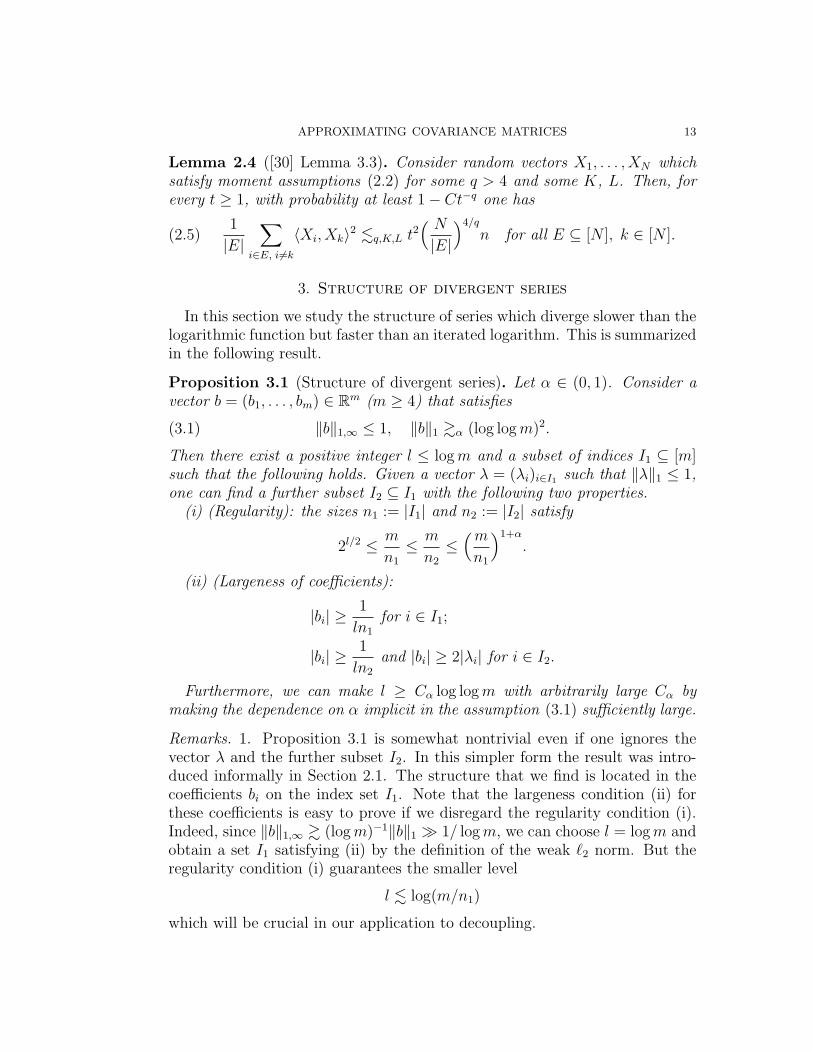
Lemma 2.4 ([30] Lemma 3.3). Consider random vectors X1, . . . , XN whichsatisfy moment assumptions (2.2) for some q > 4 and some K, L. Then, forevery t ≥ 1, with probability at least 1− Ct−q one has
(2.5)1
|E|∑
i∈E, i 6=k
〈Xi, Xk〉2 .q,K,L t2( N|E|
)4/q
n for all E ⊆ [N ], k ∈ [N ].
3. Structure of divergent series
In this section we study the structure of series which diverge slower than thelogarithmic function but faster than an iterated logarithm. This is summarizedin the following result.
Proposition 3.1 (Structure of divergent series). Let α ∈ (0, 1). Consider avector b = (b1, . . . , bm) ∈ Rm (m ≥ 4) that satisfies
(3.1) ‖b‖1,∞ ≤ 1, ‖b‖1 &α (log logm)2.
Then there exist a positive integer l ≤ logm and a subset of indices I1 ⊆ [m]such that the following holds. Given a vector λ = (λi)i∈I1 such that ‖λ‖1 ≤ 1,one can find a further subset I2 ⊆ I1 with the following two properties.
(i) (Regularity): the sizes n1 := |I1| and n2 := |I2| satisfy
2l/2 ≤ m
n1
≤ m
n2
≤(mn1
)1+α
.
(ii) (Largeness of coefficients):
|bi| ≥1
ln1
for i ∈ I1;
|bi| ≥1
ln2
and |bi| ≥ 2|λi| for i ∈ I2.
Furthermore, we can make l ≥ Cα log logm with arbitrarily large Cα bymaking the dependence on α implicit in the assumption (3.1) sufficiently large.
Remarks. 1. Proposition 3.1 is somewhat nontrivial even if one ignores thevector λ and the further subset I2. In this simpler form the result was intro-duced informally in Section 2.1. The structure that we find is located in thecoefficients bi on the index set I1. Note that the largeness condition (ii) forthese coefficients is easy to prove if we disregard the regularity condition (i).Indeed, since ‖b‖1,∞ & (logm)−1‖b‖1 1/ logm, we can choose l = logm andobtain a set I1 satisfying (ii) by the definition of the weak `2 norm. But theregularity condition (i) guarantees the smaller level
l . log(m/n1)
which will be crucial in our application to decoupling.

14 ROMAN VERSHYNIN
2. The freedom to choose λ in Proposition 3.1 ensures that the structurelocated in the set I1 is in a sense hereditary; it can pass to subsets I2. Thedomination of λ by b on I2 will be crucial in the removal of the diagonal termsin our application to decoupling.
We now turn to the proof of Proposition 3.1. Heuristically, we will first findmany (namely, l) sets I1 on which the coefficients are large as in (ii), thenchoose one that satisfies the regularity condition (i). This regularization stepwill rely on the following elementary lemma.
Lemma 3.2 (Regularization). Let N be a positive integer. Consider a nonemptysubset J ⊂ [L] with size l := |J |. Then, for every α ∈ (0, 1), there exist ele-ments j1, j2 ∈ J that satisfy the following two properties.
(i) (Regularity):
l/2 ≤ j1 ≤ j2 ≤ (1 + α)j1.
(ii) (Density):
|J ∩ [j1, j2]| &αl
log(2L/l).
Proof. We will find j1, j2 as some consecutive terms of the following geometricprogression. Define j(0) ∈ J to be the (unique) element such that
|J ∩ [1, j(0)]| = dl/2e, and let j(k) := (1 + α)j(k−1), k = 1, 2, . . . .
We will only need to consider K terms of this progression, where K := mink :j(k) ≥ L. Since j(0) ≥ dl/2e ≥ l/2, we have j(k) ≥ (1 + α)kj(0) ≥ (1 + α)kl/2.On the other hand, j(K−1) ≤ L. It follows that K .α log(2L/l).
We claim that there exists a term 1 ≤ k ≤ K such that
(3.2) |J ∩ [j(k−1), j(k)]| ≥ l
3K&α
l
log(2L/l).
Indeed, otherwise we would have
l = |J | ≤ |J ∩ [1, j(0)]|+K∑k=1
|J ∩ [j(k−1), j(k)]| ≤⌈ l
2
⌉+K · l
3K< l,
which is impossible.The terms j1 := j(k−1) and j2 := j(k) for which (3.2) holds clearly satisfy (i)
and (ii) of the conclusion. By increasing j1 and decreasing j2 if necessary wecan assume that j1, j2 ∈ J . This completes the proof.
Proof of Proposition 3.1. We shall prove the following slightly stronger state-ment. Consider a sufficiently large number
K &α log logm.

APPROXIMATING COVARIANCE MATRICES 15
Assume that the vector b satisfies
‖b‖1,∞ ≤ 1, ‖b‖1 &α K log logm.
We shall prove that the conclusion of the Proposition holds with (ii) replacedby:
|bi| ≥K
2ln1
for i ∈ I1;(3.3)
|bi| ≥K
2ln2
≥ 2|λi| for i ∈ I2.(3.4)
We will construct I1 and I2 in the following way. First we decompose theindex set [m] into blocks Ω1, . . . ,ΩL on which the coefficients bi have similarmagnitude; this is possible with L ∼ logm blocks. Using the assumption‖b‖1 & (log logm)2, one easily checks that many (at least l ∼ log logm) ofthe blocks Ωj have large contribution (at least 1/j) to the sum ‖b‖1 =
∑i |bi|.
We will only focus on such large blocks in the rest of the argument. At thispoint, the union of these blocks could be declared I1. We indeed proceed thisway, except we first use Regularization Lemma 3.2 on these blocks in orderto obtain the required regularity property (ii). Finally, assume we are givencoefficients (λi)i∈I1 with small sum
∑|λi| ≤ 1 as in the assumption. Since
the coefficients bi are large on I1 by construction, the pigeonhole principle willyield (loosely speaking) a whole block of coefficients Ωj where bi will dominateas required, |bi| ≥ 2|λi|. We declare this block I2 and complete the proof. Nowwe pass to the details of the argument.
Step 1: decomposition of [m] into blocks. Without loss of generality,
1
m< bi ≤ 1, λi ≥ 0 for all i ∈ [m].
Indeed, we can clearly assume that bi ≥ 0 and λi ≥ 0. The estimate bi ≤ 1follows from the assumption: ‖b‖∞ ≤ ‖b‖1,∞ ≤ 1. Furthermore, the contribu-tion of the small coefficients bi ≤ 1/m to the norm ‖b‖1 is at most 1, whileby the assumption ‖b‖1 &α K log logm ≥ 2. Hence we can ignore these smallcoefficients by replacing [m] with the subset corresponding to the coefficientsbi ≥ 1/m.
We decompose [m] into disjoint subsets (which we call blocks) according tothe magnitude of bi, and we consider the contribution of each block Ωj to thenorm ‖b‖1:
Ωj :=i ∈ [m] : 2−j < bi ≤ 2−j+1
; mj := |Ωj|; Bj :=
∑i∈Ωj
bi.

16 ROMAN VERSHYNIN
By our assumptions on b, there are at most logm nonempty blocks Ωj. As‖b‖1,∞ ≤ 1, Markov’s inequality yields for all j that
mj ≤∑k≤j
mk =∣∣i ∈ [m] : bi > 2−j
∣∣ ≤ 2j;(3.5)
Bj ≤ mj2−j+1 ≤ 2.(3.6)
Only the blocks with large contributions Bj will be of interest to us. Theirnumber is
l := maxj ∈ [logm] : B∗j ≥ K/j
;
and we let l = 0 if it happens that all Bj < K/j. We claim that there aremany such blocks:
(3.7)1
5K log logm ≤ l ≤ logm.
Indeed, by the assumption and using (3.6) we can bound
K log logm ≤ ‖b‖1 =
logm∑j=1
B∗j ≤ 2l + 0.6K log logm,
which yields (3.7).
Step 2: construction of the set I1. As we said before, we are onlyinterested in blocks Ωj with large contributions Bj. We collect the indices ofsuch blocks into the set
J :=j ∈ [logm] : Bj ≥ K/l
.
Since the definition of l implies that B∗l ≥ K/l, we have |J | ≥ l. Then we canapply Regularization Lemma 3.2 to the set logm − j : j ∈ J ⊆ [logm].Thus we find two elements j′, j′′ ∈ J satisfying
(3.8) l/2 ≤ logm− j′ ≤ logm− j′′ ≤ (1 + α/2)(logm− j′),and such that the set
J := J ∩ [j′′, j′]
has size |J | &α l/ log logm. Since by our choice of K we can assume thatK ≥ 8 log logm, we obtain
(3.9) |J | ≥ 8l
K.
We are going to show that the set
I1 :=⋃j∈J
Ωj
satisfies the conclusion of the Proposition.

APPROXIMATING COVARIANCE MATRICES 17
Step 3: sizes of the coefficients bi for i ∈ I1. Let us fix j ∈ J ⊆ J .From the definition of J we know that the contribution Bj is large: Bj ≥ K/l.One consequence of this is a good estimate of the size mj of the block Ωj.Indeed, the above bound together with (3.6) this implies
(3.10)K
2l2j ≤ mj ≤ 2j for j ∈ J.
Another consequence of the lower bound on Bj is the required lower bound onthe individual coefficients bi. Indeed, by construction of Ωj the coefficients bi,i ∈ Ωj are within the factor 2 from each other. It follows that
(3.11) bi ≥1
2|Ωj|∑i∈Ωj
bi =Bj
2mj
≥ K
2lmj
for i ∈ Ωj, j ∈ J.
In particuar, since by construciton Ωj ⊆ I1, we have mj ≤ |I1|, which implies
bi ≥K
2l|I1|for i ∈ I1.
We have thus proved the required lower bound (3.3).
Step 4: Construction of the set I2, and sizes of the coefficients bifor i ∈ I2. Now suppose we are given a vector λ = (λi)i∈I1 with ‖λ‖1 ≤ 1.We will have to construct a subset I2 ⊂ I1 as in the conclusion, and we will dothis as follows. Consider the contribution of the block Ωj to the norm ‖λ‖1:
Lj :=∑i∈Ωj
λj, j ∈ J.
On the one hand, the sum of all contributions is bounded as∑
j∈J Lj = ‖λ‖1 ≤1. On the other hand, there are many terms in this sum: |J | ≥ 8l/K as weknow from (3.9). Therefore, by the pigeonhole principle some of the contribu-tions must be small: there exists j0 ∈ J such that
Lj0 ≤ K/8l.
This in turn implies via Markov’s inequality that most of the coefficients λifor i ∈ Ωj0 are small, and we shall declare these set of indices I2. Specifically,since Lj0 =
∑i∈Ωj0
λj ≤ K/8l and |Ωj0| = mj0 , using Markov’s inequality we
see that the set
I2 :=i ∈ Ωj0 : λi ≤
K
4lmj0
has cardinality
(3.12)1
2mj0 ≤ |I2| ≤ mj0 .

18 ROMAN VERSHYNIN
Moreover, using (3.11), we obtain
bi ≥K
2lmj0
≥ 2λi for i ∈ I2.
We have thus proved the required lower bound (3.4).
Step 5: the sizes of the sets I1 and I2. It remains to check the regularityproperty (i) of the conclusion of the Proposition. We bound
|I1| =∑j∈J
mj (by definition of I1)
≤∑j≤j′
mj (by definition of J)
≤ 2j. (by (3.5))
Therefore, using (3.8) we conclude that
(3.13)m
|I1|≥ 2logm−j′ ≥ 2l/2.
We have thus proved the first inequality in (i) of the conclusion of the Propo-sition. Similarly, we bound
|I2| ≥1
2mj0 (by (3.12))
≥ K
4l2j0 (by (3.10), and since j0 ∈ J)
≥ K
4l2j′′. (by definition of J , and since j0 ∈ J)
Therefore
m
|I2|≤ 4l
K2logm−j′′
≤ 8
K(logm− j′)2(1+α/2)(logm−j′) (by (3.8))
≤ α
2(logm− j′)2(1+α/2)(logm−j′) (by the assumption on K)
≤ 2(1+α)(logm−j′)
≤( m|I1|
)1+α
. (by (3.13))
This completes the proof of (i) of the conclusion, and of the whole Proposi-tion 3.1.
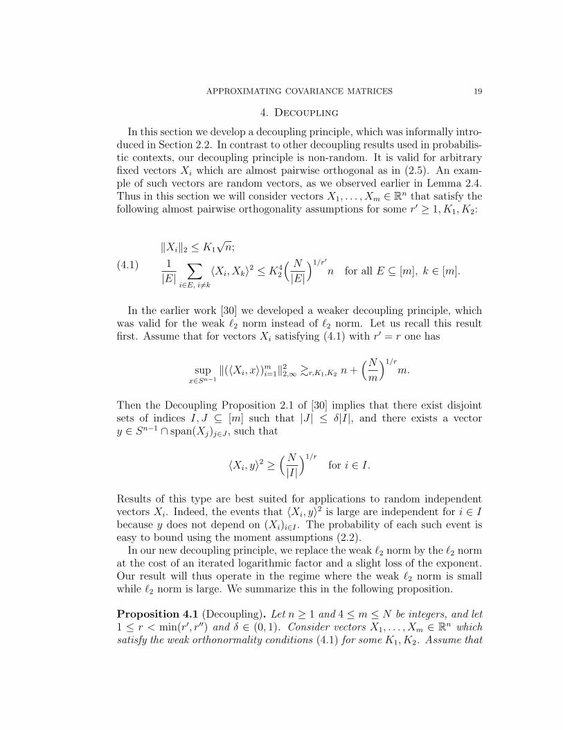
APPROXIMATING COVARIANCE MATRICES 19
4. Decoupling
In this section we develop a decoupling principle, which was informally intro-duced in Section 2.2. In contrast to other decoupling results used in probabilis-tic contexts, our decoupling principle is non-random. It is valid for arbitraryfixed vectors Xi which are almost pairwise orthogonal as in (2.5). An exam-ple of such vectors are random vectors, as we observed earlier in Lemma 2.4.Thus in this section we will consider vectors X1, . . . , Xm ∈ Rn that satisfy thefollowing almost pairwise orthogonality assumptions for some r′ ≥ 1, K1, K2:
‖Xi‖2 ≤ K1
√n;
1
|E|∑
i∈E, i 6=k
〈Xi, Xk〉2 ≤ K42
( N|E|
)1/r′
n for all E ⊆ [m], k ∈ [m].(4.1)
In the earlier work [30] we developed a weaker decoupling principle, whichwas valid for the weak `2 norm instead of `2 norm. Let us recall this resultfirst. Assume that for vectors Xi satisfying (4.1) with r′ = r one has
supx∈Sn−1
‖(〈Xi, x〉)mi=1‖22,∞ &r,K1,K2 n+
(Nm
)1/r
m.
Then the Decoupling Proposition 2.1 of [30] implies that there exist disjointsets of indices I, J ⊆ [m] such that |J | ≤ δ|I|, and there exists a vectory ∈ Sn−1 ∩ span(Xj)j∈J , such that
〈Xi, y〉2 ≥(N|I|
)1/r
for i ∈ I.
Results of this type are best suited for applications to random independentvectors Xi. Indeed, the events that 〈Xi, y〉2 is large are independent for i ∈ Ibecause y does not depend on (Xi)i∈I . The probability of each such event iseasy to bound using the moment assumptions (2.2).
In our new decoupling principle, we replace the weak `2 norm by the `2 normat the cost of an iterated logarithmic factor and a slight loss of the exponent.Our result will thus operate in the regime where the weak `2 norm is smallwhile `2 norm is large. We summarize this in the following proposition.
Proposition 4.1 (Decoupling). Let n ≥ 1 and 4 ≤ m ≤ N be integers, and let1 ≤ r < min(r′, r′′) and δ ∈ (0, 1). Consider vectors X1, . . . , Xm ∈ Rn whichsatisfy the weak orthonormality conditions (4.1) for some K1, K2. Assume that

20 ROMAN VERSHYNIN
for some K3 ≥ max(K1, K2) one has
supx∈Sn−1
‖(〈Xi, x〉)mi=1‖22,∞ ≤ K2
3
[n+
(Nm
)1/r
m],(4.2)
∥∥∥ m∑i=1
Xi ⊗Xi
∥∥∥ = supx∈Sn−1
m∑i=1
〈Xi, x〉2 &r,r′,r′′,δ K23(log logm)2
[n+
(Nm
)1/r
m].
(4.3)
Then there exist nonempty disjoint sets of indices I, J ⊆ [m] such that |J | ≤δ|I|, and there exists a vector y ∈ Sn−1 ∩ span(Xj)j∈J , such that
〈Xi, y〉2 ≥ K23
(N|I|
)1/r′′
for i ∈ I.
The proof of the Decoupling Proposition 4.1 will use Proposition 3.1 inorder to locate the structure of the large coefficients 〈Xi, x〉. The followingelementary lemma will be used in the argument.
Lemma 4.2. Consider a vector λ = (λ1, . . . , λn) ∈ Rn which satisfies
‖λ‖1 ≤ 1, ‖λ‖∞ ≤ 1/K
for some integer K. Then, for every real numbers (a1, . . . , an) ∈ Rn one has
n∑i=1
λiai ≤1
K
K∑i=1
a∗i .
Proof. It is easy to check that each extreme point of the convex set
Λ := λ ∈ Rn : ‖λ‖1 ≤ 1, ‖λ‖∞ ≤ 1/Khas exactly K nonzero coefficients which are equal to ±1/K. Evaluating thelinear form
∑λiai on these extreme points, we obtain
supλ∈Λ
n∑i=1
λiai = supλ∈ext(Λ)
n∑i=1
λiai =1
K
K∑i=1
a∗i .
The proof is complete.
Proof of Decoupling Proposition 4.1. By replacing Xi with Xi/K3 we can as-sume without loss of generality that K1 = K2 = K3 = 1. By perturbing thevectors Xi slightly we may also assume that Xi are all different.
Step 1: separation and the structure of coefficients. Suppose theassumptions of the Proposition hold, and let us choose a vector x ∈ Sn−1
which attains the supremum in (4.3). We denote
ai := 〈Xi, x〉 for i ∈ [m],

APPROXIMATING COVARIANCE MATRICES 21
and without loss of generality we may assume that ai 6= 0. We also denote
n := n+(Nm
)1/r
m.
We choose parameter α = α(r, r′, r′′, δ) ∈ (0, 1) sufficiently small; its choicewill become clear later on in the argument. At this point, we may assume that
‖a‖22,∞ ≤ n, ‖a‖2
2 &α (log logm)2n.
We can use Structure Proposition 3.1 to locate the structure in the coefficientsai. To this end, we apply this result for bi = a2
i /n and obtain a numberl ≤ logm and a subset of indices I1 ⊆ [m]. We can also assume that l issufficiently large – larger than an arbitrary quantity which depends on α.
Since a vector x ∈ Sn−1 satisfies 〈Xi/ai, x〉 = 1 for all i ∈ I1 (in fact forall i ∈ [m]), a separation argument for the convex hull K := conv(Xi/ai)i∈I1yields the existence of a vector x ∈ conv(K ∪ 0) that satisfies
(4.4) ‖x‖2 = 1, 〈Xi/ai, x〉 ≥ 1 for i ∈ I1.
We express x as a convex combination
(4.5) x =∑i∈I1
λiXi/ai for some λi ≥ 0,∑i∈I1
λi ≤ 1.
We then read the conclusion of Structure Proposition 3.1 as follows. Thereexists a futher subset of indices I2 ⊆ I1 such that the sizes n1 := |I1| andn2 := |I2| are regular in the sense that
(4.6) 2l/2 ≤ m
n1
≤ m
n2
≤(mn1
)1+α
,
and the coefficients on I1 and I2 are large:
a2i ≥
n
ln1
for i ∈ I1,(4.7)
a2i ≥
n
ln2
and a2i ≥ 2λin for i ∈ I2.(4.8)
Furthermore, we can make l sufficiently large depending on α, say l ≥ 100/α2.
Step 2: random selection. We will reduce the number of terms n1 inthe sum (4.5) defining x using random selection, trying to bring this numberdown to about n2. As is usual in dealing with sums of independent randomvariables, we will need to ensure that all summands λiXi/ai have controlledmagnitudes. To this end, we have ‖Xi‖2 ≤
√n by the assumption, and we can
bound 1/ai through (4.7). Finally, we have an a priori bound λi ≤ 1 on thecoefficients of the convex combination. However, the latter bound will turn outto be too weak, and we will need λi .α 1/n2 instead. To make this happen,

22 ROMAN VERSHYNIN
instead of the sets I1 and I2 we will be working on their large subsets I ′1 andI ′2 defines as
I ′1 :=i ∈ I1 : λi ≤
Cαn2
, I ′2 :=
i ∈ I2 : λi ≤
Cαn2
where Cα is a sufficiently large quantity whose value we will choose later. ByMarkov’s inequality, this incurs almost no loss of coefficients:
(4.9) |I1 \ I ′1| ≤n2
Cα, |I2 \ I ′2| ≤
n2
Cα.
We will perform a random selection on I1 using B. Maurey’s empiricalmethod [21]. Guided by the representation (4.5) of x as a convex combi-nation, we will treat λi as probabilities, thus introducing a random vector Vwith distribution
PV = Xi/ai = λi, i ∈ I ′1.
On the remainder of the probability space, we assign V zero value: PV =0 = 1 −
∑i∈I′1
λi. Consider independent copies V1, V2, . . . of V . We are not
going to do a random selection on the set I1 \ I ′1 where the coefficients λi maybe out of control, so we just add its the contribution by defining independentrandom vectors
Yj := Vj +∑
i∈I1\I′1
λiXiai, j = 1, 2, . . .
Finally, for C ′α := Cα/α, we consider the average of about n2 such vectors:
(4.10) y :=C ′αn2
n2/C′α∑j=1
Yj.
We would like to think of y as a random version of the vector x. This iscertainly true in expectation:
Ey = EY1 =∑i∈I1
λiXi/ai = x.
Also, like x, the random vector y is a convex combination of terms Xi/ai (noweven with equal weights). The advantage of y over x is that it is a convexcombination of much fewer terms, as n2/C
′α n2 ≤ n1. In the next two
steps, we will check that y is similar to x in the sense that its norm is alsowell bounded above, and at least ∼ n2 of the inner products 〈Xi/ai, y〉 are stillnicely bounded below.

APPROXIMATING COVARIANCE MATRICES 23
Step 3: control of the norm. By independence, we have
E‖y − x‖22 = E
∥∥∥C ′αn2
n2/C′α∑j=1
(Yj − EYj)∥∥∥2
2=(C ′αn2
)2n2/C′α∑j=1
E‖Yj − EYj‖22
.α1
n2
E‖Y1 − EY1‖22 =
1
n2
E‖V − EV ‖22 ≤
4
n2
E‖V ‖22
=4
n2
∑i∈I′1
λi‖Xi‖22/a
2i ≤
4
n2
maxi∈I1‖Xi‖2
2/a2i ,
where the last inequality follows because I ′1 ⊆ I1 and∑
i∈I1 λi ≤ 1.Since n ≥ n, (4.7) gives us the lower bound
a2i ≥
n
ln1
for i ∈ I1.
Together with the assumption ‖Xi‖22 ≤ n, this implies that
E‖y − x‖22 .α
1
n2
· n
n/ln1
≤ ln1
n2
.
Since ‖x‖22 = 1 ≤ ln1/n2, we conclude that with probability at least 0.9, one
has
(4.11) ‖y‖22 .α
ln1
n2
.
Step 4: removal of the diagonal term. We know from (4.4) that〈Xi/ai, x〉 ≥ 1 for many terms Xi. We would like to replace x by its ran-dom version y, establishing a lower bound 〈Xk/ak, y〉 ≥ 1 for many terms Xk.But at the same time, our main goal is decoupling, in which we would needto make the random vector y independent of those terms Xk. To make thispossible, we will first remove from the sum (4.10) defining y the “diagonal”term containing Xk, and we call the resulting vector y(k).
To make this precise, let us fix k ∈ I ′2 ⊆ I ′1 ⊆ I1. We consider independentrandom vectors
V(k)j := Vj1Vj 6=Xk/ak, Y
(k)j := V
(k)j +
∑i∈I1\I′1
λiXiai, j = 1, 2, . . .
Note that
(4.12) PY (k)j 6= Yj = PV (k)
j 6= Vj = PVj = Xk/ak = λk.
Similarly to the definition (4.10) of y, we define
y(k) :=C ′αn2
n2/C′α∑j=1
Y(k)j .

24 ROMAN VERSHYNIN
Then
(4.13) Ey(k) = EY (k)1 = EY1 − λkXk/ak = x− λkXk/ak.
As we said before, we would like to show that the random variable
Zk := 〈Xk/ak, y(k)〉
is bounded below by a constant with high probability. First, we will estimateits mean
EZk = 〈Xk/ak, x〉 − λk‖Xk‖22/a
2k.
To estimate the terms in the right hand side, note that 〈Xi/ai, x〉 ≥ 1 by (4.4)and ‖Xk‖2
2 ≤ n by the assumption. Now is the crucial point when we use thata2i dominate λi as in the second inequality in (4.8). This allows us to bound
the “diagonal” term as
λk‖Xk‖22/a
2k ≤ n/2n ≤ n/2n = 1/2.
As a result, we have
(4.14) EZk ≥ 1− 1/2 = 1/2.
Step 5: control of the inner products. We would need a strongerstatement than (4.14) – that Zk is bounded below not only in expectationbut also with high probability. We will get this immediately by Chebyshev’sinequality if we can upper bound the variance of Zk. In a way similar to Step 3,we estimate
VarZk = E(Zk − EZk)2 = E⟨Xk/ak,
C ′αn2
n2/C′α∑j=1
(Y(k)j − EY (k)
j )⟩2
.α1
n2
E〈Xk/ak, V(k)
1 〉2 =1
n2
∑i∈I′1, i 6=k
λi〈Xk/ak, Xi/ai〉2.(4.15)
Now we need to estimate the various terms in the right hand side of (4.15).We start with the estimate on the inner products, collecting them into
S :=∑
i∈I′1, i 6=k
λi〈Xk, Xi〉2 =∑i∈I′1
λipki where pki = 〈Xk, Xi〉21k 6=i.
Recall that, by the construction of λi and of I ′1 ⊆ I, we have∑
i∈I′1λi ≤ 1 and
λi ≤ Cα/n2 for i ∈ I ′1. We use Lemma 4.2 on order statistics to obtain thebound
S ≤ Cαn2
n2/Cα∑i=1
(pk)∗i =
Cαn2
maxE⊆[m]
|E|=n2/Cα
∑i∈E, i 6=k
〈Xi, Xk〉2.

APPROXIMATING COVARIANCE MATRICES 25
Finally, we use our weak orthonormality assumption (4.1) to conclude that
S .α(Nn2
)1/r′
n.
To complete the bound on the variance of Zk in (4.15) it remains to obtainsome good lower bounds on ak and ai. Since k ∈ I ′2 ⊆ I2, (4.8) yields
a2k ≥
n
ln2
≥ n
ln2
.
Similarly we can bound the coefficients ai in (4.15): using (4.7) we have a2i ≥
n/ln1 since since i ∈ I ′1 ⊆ I. But here we will not simply replace n by n, as weshall try to use a2
i to offset the term (N/n2)1/r′ in the estimate on S. To thisend, we note that n ≥ (N/m)1/rm ≥ (N/n1)1/rn1 because m ≥ n1. Therefore,using the last inequality in (4.6) and that N ≥ m, we have
(4.16)n
n1
≥(Nn1
)1/r
≥(Nn2
) 1(1+α)r
.
Using this, we obtain a good lower bound
a2i ≥
n
ln1
≥ 1
l
(Nn2
) 1(1+α)r
, for i ∈ I ′1.
Combining the estimates on S, ak and ai, we conclude our lower bound(4.15) on the variance of Zk as follows:
VarZk .α1
n2
· ln2
n· l(n2
N
) 1(1+α)r ·
(Nn2
)1/r′
n
≤ l2(n2
N
)α(by choosing α small enough depending on r, r′)
≤ l2(n2
m
)α≤ l22−αl/2 (by (4.6))
≤ α/16. (since l is large enough depending on α)
Combining this with the lower bound (4.14) on the expectation, we concludeby Chebyshev’s inequality the desired estimate
(4.17) PZk = 〈Xk/ak, y
(k)〉 ≥ 1
4
≥ 1− α for k ∈ I ′2.
Step 6: decoupling. We are nearing the completion of the proof. Let usconsider the good events
Ek :=〈Xk/ak, y〉 ≥
1
4and y = y(k)
for k ∈ I ′2.

26 ROMAN VERSHYNIN
To show that each Ek occurs with high probability, we note that by definitionof y and y(k) one has
Py 6= y(k) ≤ PYj 6= Y(k)j for some j ∈ [n2/C
′α]
≤n2/C′α∑j=1
PYj 6= Y(k)j =
n2
C ′α· λk (by (4.12))
≤ n2
C ′α· Cαn2
(by definition of I ′2)
= α. (as we chose C ′α = Cα/α)
From this and using (4.17) we conclude that
PEk ≥ 1− P〈Xk/ak, y
(k)〉 < 1
4
− Py 6= y(k) ≥ 1− 2α for k ∈ I ′2.
An application of Fubini theorem yields that with probability at least 0.9,at least (1 − 20α)|I ′2| of the events Ek hold simultaneously. More accurately,with probability at least 0.9 the following event occurs, which we denote by E .There exists a subset I ⊆ I ′2 of size |I| ≥ (1 − 20α)|I ′2| such that Ek holds forall k ∈ I. Note that using (4.9) and choosing Cα sufficiently large we have
(4.18) (1− 21α)n2 ≤ |I| ≤ n2.
Recall that the norm bound (4.11) also holds with high probability 0.9.Hence with probability at least 0.8, both E and this norm bound holds. Let usfix a realization of our random variables for which this happens. Then, first ofall, by definition of Ek we have
(4.19) 〈Xk/ak, y〉 ≥1
4for k ∈ I.
Next, we are going to observe that y lies in the span of few vectors Xi. Indeed,
by construction y(k) lies in the span of the vectors Y(k)j for j ∈ [n2/C
′α]. Each
such Y(k)j by construction lies in the span of the vectors Xi, i ∈ I1 \ I ′1 and of
one vector V(k)j . Finally, each such vector V
(k)j , again by construction, is either
equal zero or Vj, which in turn equals Xi0 for some i0 6= k. Since E holds, wehave y = y(k) for all k ∈ I. This implies that there exists a subset I0 ⊆ [m](consisting of the indices i0 as above) with the following properties. Firstly,I0 does not contain any of indices k ∈ I; in other words I0 is disjoint from I.Secondly, this set is small: |I0| ≤ n2/C
′α. Thirdly, y lies in the span of Xi,
i ∈ I0 ∪ (I1 \ I ′1). We claim that this set of indices,
J := I0 ∪ (I1 \ I ′1)
satisfies the conclusion of the Proposition.

APPROXIMATING COVARIANCE MATRICES 27
Since I and I0 are disjoint and I ⊆ I ′2 ⊆ I ′1, it follows that I and J aredisjoint as required. Moreover, by (4.9) and by choosing Cα, C ′α sufficientlylarge we have
|J | ≤ |I0|+ |I1 \ I ′1| ≤n2
C ′α+n2
Cα≤ αn2.
When we combine this with (4.18) and choose α sufficiently small dependingon δ, we achieve
|J | ≤ δ|I|as required. Finally, we claim that the normalized vector
y :=y
‖y‖2
satisfies the conclusion of the Proposition. Indeed, we already noted thaty ∈ span(Xj)j∈J , as required. Next, for each k ∈ I ⊆ I ′2 ⊆ I2 we have
〈Xk, y〉2 ≥a2k
16‖y‖22
(by (4.19))
&αn
ln2
· n2
ln1
(by (4.8) and (4.11))
=n
l2n1
≥ 1
l2
(Nn2
) 1(1+α)r
. (by (4.16))
We can get rid of l2 in this estimate using the bound(Nn2
) α(1+α)r ≥
(mn2
) α(1+α)r ≥ 2
αl2(1+α)r (by (4.6))
≥ 2αl3r ≥ 2α
2l (choosing α small enough depending on r)
≥ l2. (since l is large enough depending on α)
Therefore
〈Xk, y〉2 ≥(Nn2
) 1−α(1+α)r ≥
(Nn2
)1/r′′
for k ∈ I
where the last inequality follows by choosing α sufficiently small depending onr, r′′. This completes the proof of Decoupling Proposition 4.1.
5. Norms of random matrices with independent columns
In this section we apply our decoupling principle, Proposition 4.1, to es-timate norms of random matrices with independent columns. As we said,a simple truncation argument of J. Bourgain [6] reduces the approximationproblem for covariance matrices to bounding the norm of the random matrix∑
i∈E Xi ⊗Xi uniformly over index sets E. The following result gives such anestimate for random vectors Xi with finite moment assumptions.

28 ROMAN VERSHYNIN
Theorem 5.1. Let 1 ≤ n ≤ N be integers, and let 4 < p < q and t ≥1. Consider independent random vectors X1, . . . , XN in Rn (1 ≤ n ≤ N)which satisfy the moment assumptions (2.2). Then with probability at least1− Ct−0.9q, for every index set E ⊆ [N ], |E| ≥ 4, one has∥∥∥∑
i∈E
Xi ⊗Xi
∥∥∥ .p,q,K,L t2(log log |E|)2[n+
( N|E|
)4/p
|E|].
We can state Theorem 5.1 in terms of random matrices with independentcolumns.
Corollary 5.2. Let 1 ≤ n ≤ N be integers, and let 4 < p < q and t ≥ 1.Consider the n×N random matrix A whose columns are independent randomvectors X1, . . . , XN in Rn which satisfy (2.2). Then with probability at least1− Ct−0.9q one has
‖A‖ .p,q,K,L t log logN · (√n+√N).
Moreover, with the same probability all n×m submatrices B of A simultane-ously satisfy the following for all 4 ≤ m ≤ N :
‖B‖ .p,q,K,L t log logm ·[√
n+(Nm
)2/p√m].
Proof of Theorem 5.1. By replacing Xi with Xi/max(K,L) we can assumewithout loss of generality that K = L = 1. As we said, the argument willbe based on Decoupling Proposition 4.1. Its assumptions follow from knownresults. Indeed, the pairwise almost orthogonality of the vectors Xi followsfrom Lemma 2.4, which yields (2.5) with probability at least 1 − Ct−q. Also,the required bound on the weak `2 norm follows from Theorem 2.3, which giveswith probability at least 1− Ct−0.9q that
(5.1) supx∈Sn−1
‖(〈Xi, x〉)i∈I‖22,∞ .q t
2[n+
(N|I|
)4/q
|I|]
for I ⊆ [N ].
Consider the event E that both required bounds (2.5) and (5.1) hold.Let E0 denote the event in the conclusion of the Theorem. It remains to
prove that P(Ec0 and E) is small. To this end, assume that E holds but E0 doesnot. Then there exists an index set E ⊂ [N ] whose size we denote by m := |E|,and which satisfies∥∥∥∑
i∈E
Xi ⊗Xi
∥∥∥ = supx∈Sn−1
∑i∈E
〈Xi, x〉2 &p,q t2(log logm)2[n+
(Nm
)4/p
m].
Recalling (2.5) and (5.1) we see that the assumptions of Decoupling Proposi-tion 4.1 hold for 1/r = 4/p, 1/r′ = 4/q, r′′ = r′, K1 = K = 1, K2 = Cq
√t

APPROXIMATING COVARIANCE MATRICES 29
for suitably large Cq, K3 = max(K1, K2, 100t2), and for δ = δ(p, q) > 0 suf-ficiently small (to be chosen later). Applying Decoupling Proposition 4.1 weobtain disjoint index sets I, J ⊆ E ⊆ [N ] with sizes
|I| =: s, |J | ≤ δs,
and a vector y ∈ Sn−1 ∩ span(Xj)j∈J such that
(5.2) 〈Xi, y〉2 ≥ 100t2(Ns
)1/r′′
for i ∈ I.
We will need to discretize the set of possible vectors y. Let
ε :=(δsN
)5
and consider an ε-net NJ of the sphere Sn−1 ∩ span(Xj)j∈J . As in known bya volumetric argument (see e.g. [19] Lemma 2.6), one can choose such a netwith cardinality
|NJ | ≤ (3/ε)|J | ≤(2N
δs
)5δs
.
We can assume that the random set NJ depends only on the number ε, theset J and the random variables (Xj)j∈J . Given a vector y as we have foundabove, we can approximate it with some vector y0 ∈ NJ so that ‖y− y0‖2 ≤ ε.By (5.1) we have
‖(〈Xi, y − y0〉)i∈I‖22,∞ .q ε
2t2[n+
(Ns
)1/r′
s].
This implies that all but at most δs indices i in I satisfy the inequality
(5.3) 〈Xi, y − y0〉2 .qε2t2
δs
[n+
(Ns
)1/r′
s].
Let us denote the set of these indices by I0 ⊆ I. The bound in (5.3) can besimplified as
ε2
δs
[n+
(Ns
)1/r′
s]≤ 2δ.
Indeed, this estimate follows from the two bounds
ε2
δs· n ≤
(δsN
)10
· nδs≤ δ (because n ≤ N);
ε2
δs·(Ns
)1/r′
s ≤ 1
δ
(δsN
)10(Ns
)1/r′
≤ δ. (because δ ≤ 1, r′ ≥ 1)
In particular, by choosing δ = δ(q) > 0 sufficiently small, (5.3) implies
|〈Xi, y − y0〉| ≤ t for i ∈ I0.
Together with (5.2) this yields by triangle inequality that
|〈Xi, y0〉| ≥ 10t(Ns
)1/2r′′
− t ≥ 9t(Ns
)1/2r′′
for i ∈ I0.

30 ROMAN VERSHYNIN
Summarizing, we have shown that the event Ec0 and E implies the followingevent: there exists a number s ≤ N , disjoint index subsets I0, J ⊆ [N ] withsizes |I0| ≥ (1− δ)s, |J | ≤ δs, and a vector y0 ∈ NJ such that
|〈Xi, y0〉| ≥ 9t(Ns
)1/2r′′
for i ∈ I0.
It will now be easy to estimate the probability of this event. First of all, foreach fixed vector y0 ∈ Sn−1 and each index i, the moment assumptions (2.2)imply via Markov’s inequality that
P|〈Xi, y0〉| ≥ 9t
(Ns
)1/2r′′≤ 1
(9t)q
(Ns
)−q/2r′′≤ 1
9tq
(Ns
)−2
where the last line follows from our choice of q and r′′. By independence, foreach fixed vector y0 ∈ Sn−1 and a fixed index set I0 ⊆ [N ] of size |I0| ≥ (1−δ)swe have
P|〈Xi, y0〉| ≥ 9
(Ns
)1/2r′′
for i ∈ I0
≤[ 1
9tq
(Ns
)−2]|I0|≤ 9−(1−δ)st−(1−δ)q
(Ns
)−2(1−δ)s.(5.4)
Then we bound the probability of event Ec0 and E by taking the union boundover all s, I0, J as above, conditioning on the random variables (Xj)j∈J (whichfixes the ε-net NJ), taking the union bound over the choice of y0 ∈ NJ , andfinally evaluating the probability for using (5.4). This way we obtain viaStirling’s approximation of the binomial coefficients that
PEc0 and E ≤N∑s=1
(N
|I0|
)(N
|J |
)|NJ | 9−(1−δ)st−(1−δ)q
(Ns
)−2(1−δ)s
≤ t−(1−δ)qN∑s=1
( eN
(1− δ)s
)(1−δ)s(eNδs
)δs(2N
δs
)5δs
9−(1−δ)s(Ns
)−2(1−δ)s
≤ t−0.9q
N∑s=1
(N2s
)s(by choosing δ > 0 small enough)
≤ t−0.9q.
It follows that
PEc0 ≤ PEc0 and E+ PEc ≤ t−0.9q + Ct−q + Ct−0.9q . t−0.9q.
This completes the proof of Theorem 5.1.

APPROXIMATING COVARIANCE MATRICES 31
6. Approximating covariance matrices
In this final section, we deduce our main result on the approximation ofcovariance matrices for random vectors with finite moments.
Theorem 6.1. Consider independent random vectors X1, . . . , XN in Rn, 4 ≤n ≤ N , which satisfy moment assumptions (2.2) for some q > 4 and some K,L. Then for every δ > 0 with probability at least 1− δ one has
(6.1)∥∥∥ 1
N
N∑i=1
Xi ⊗Xi − EXi ⊗Xi
∥∥∥ .q,K,L,δ (log log n)2( nN
) 12− 2q.
In our proof of Theorem 6.1, we can clearly assume that K = L = 1 in themoment assumptions (2.2) by rescaling the vectors Xi. So in the rest of thissection we suppose Xi are such random vectors.
For a level B > 0 and a vector x ∈ Sn−1, we consider the (random) indexset of large coefficients
EB = EB(x) := i ∈ [N ] : |〈Xi, x〉| ≥ B.
Lemma 6.2 (Large coefficients). Let t ≥ 1. With probability at least 1−Ct0.9q,one has
|EB| .q n/B2 +N(t/B)q/2 for B > 0.
Proof. This estimate follows from Theorem 2.3. By definition of the set EBand the weak `2 norm, we obtain with the required probability that
B2|EB| ≤ ‖(〈Xi, x〉)i∈EB‖22,∞ .q n+ t2
( N
|EB|
)4/q
|EB|.
Solving for |EB| we obtain the bound as in the conclusion.
Proof of Theorem 6.1. The truncation argument described in [1] in the be-ginning of proof of Proposition 4.3 reduces the problem to estimating thecontribution to the sum of large coefficients. Denote
E =∥∥∥ 1
N
N∑i=1
Xi ⊗Xi − EXi ⊗Xi
∥∥∥ = supx∈Sn−1
∣∣∣ 1
N
N∑i=1
〈Xi, x〉2 − E〈Xi, x〉2∣∣∣.
The truncation argument yields that for every B ≥ 1, one has with probabilityat least 1− δ/3 that
E .q,δ B
√n
N+ sup
x∈Sn−1
1
N
∑i∈EB
〈Xi, x〉2 + supx∈Sn−1
1
NE∑i∈EB
〈Xi, x〉2
=: I1 + I2 + I3.(6.2)

32 ROMAN VERSHYNIN
We choose the value of the level
B =(Nn
)2/q
so that, using Lemma 6.2, with probability at least 1− δ/3 we have
(6.3) |EB| .q,δ n.It remains to estimate the right hand side of (6.2) using (6.3).
First, we clearly have
I1 =( nN
) 12− 2q.
An estimate of I2 follows from Theorem 5.1 for some p = p(q) ∈ (4, q) to bedetermined later. Note that enlarging EB can only make I2 and I3 larger.So without loss of generality we can assume that |EB| ≥ 4 as required inTheorem 5.1. This way, we obtain with probability at least 1− δ/3 that
I2 .q,δ1
N(log log |EB|)2
[n+
( N
|EB|
)4/p
|EB|]
.q,δ (log log n)2[ nN
+( nN
)1− 4p]. (by (6.3))
Finally, to estimate I3 let us fix x and consider the random variable Zi =|〈Xi, x〉|. Since EZq
i ≤ 1, an application of Holder’s and Markov’s inequalitiesyield
EZ2i 1Zi≥B ≤ (EZq
i )2/q(P(Zi ≥ B))1−2/q ≤ B2−q .q,δ
( nN
)2− 4q.
Therefore
I3 = supx∈Sn−1
1
N
N∑i=1
EZ2i 1Zi≥B .q,δ
( nN
)2− 4q.
Since we are free to choose p = p(q) in the interval (4, q), we choose themiddle of the interval, p = (q + 4)/2. Returning to (6.2) we conclude that
E .q,δ (log log n)2( nN
) 12− 2q.
This completes the proof of Theorem 6.1.
References
[1] R. Adamczak, A. Litvak, A. Pajor, N. Tomczak-Jaegermann, Quantitative estimates ofthe convergence of the empirical covariance matrix in log-concave ensembles, J. Amer.Math. Soc. 234 (2010), 535–561.
[2] R. Adamczak, A. Litvak, A. Pajor, N. Tomczak-Jaegermann, Sharp bounds on the rateof convergence of the empirical covariance matrix, preprint.
[3] G. Aubrun, Sampling convex bodies: a random matrix approach, Proc. Amer. Math.Soc. 135 (2007), 1293–1303

APPROXIMATING COVARIANCE MATRICES 33
[4] K. Ball, An elementary introduction to modern convex geometry. Flavors of geometry,1–58, Math. Sci. Res. Inst. Publ., 31, Cambridge Univ. Press, Cambridge, 1997
[5] Z. D. Bai and Y. Q. Yin, Limit of the smallest eigenvalue of a large dimensional samplecovariance matrix, Ann. Probab. 21 (1993), 1275–1294
[6] J. Bourgain, Random points in isotropic convex sets. Convex geometric analysis (Berke-ley, CA, 1996), 53–58, Math. Sci. Res. Inst. Publ., 34, Cambridge Univ. Press, Cam-bridge, 1999
[7] J. Dahmen, D. Keysers, M. Pitz, H. Ney, Structured Covariance Matrices for StatisticalImage Object Recognition. In: 22nd Symposium of the German Association for PatternRecognition. Springer, 2000, pp. 99–106
[8] A. Giannopoulos, M. Hartzoulaki, A. Tsolomitis, Random points in isotropic uncondi-tional convex bodies, J. London Math. Soc. 72 (2005), 779–798.
[9] A. Giannopoulos, V. D. Milman, Concentration property on probability spaces, Adv.Math. 156 (2000), 77–106.
[10] A. Giannopoulos, V. D. Milman, Euclidean structure in finite dimensional normedspaces. Handbook of the geometry of Banach spaces, Vol. I, 707–779, North-Holland,Amsterdam, 2001.
[11] E. Kovacevic, A. Chebira, An Introduction to Frames, Foundations and Trends in SignalProcessing, Now Publishers, 2008
[12] R. Kannan, L. Lovasz, M. Simonovits, Random walks and O∗(n5) volume algorithm forconvex bodies, Random Structures and Algorithms 2 (1997), 1–50
[13] R. Kannan, L. Rademacher, Optimization of a convex program with a polynomial per-turbation, Operations Research Letters 37(2009), 384–386
[14] H. Krim and M. Viberg, Two decades of array signal processing research: The para-metric approach, IEEE Signal Process. Mag. 13 (1996), 67–94
[15] R. Latala, Some estimates of norms of random matrices, Proc. Amer. Math. Soc. 133(2005), 1273–1282
[16] O. Ledoit, M. Wolf, Improved estimation of the covariance matrix of stock returns withan application to portfolio selection, Journal of Empirical Finance 10 (2003), 603–621
[17] M. Ledoux, M. Talagrand, Probability in Banach spaces. Isoperimetry and processes.Ergebnisse der Mathematik und ihrer Grenzgebiete (3), 23 Springer-Verlag, Berlin, 1991
[18] E. Levina, R. Vershynin, Partial estimation of covariance matrices, preprint[19] V. Milman, G. Schechtman, Asymptotic theory of finite dimensional normed spaces.
Lecture Notes in Mathematics, 1200. Springer-Verlag, Berlin, 1986[20] G. Paouris, Concentration of mass on convex bodies, Geom. Funct. Anal. 16 (2006),
1021–1049[21] G. Pisier, Remarques sur un resultat non publie de B. Maurey, Seminar on Functional
Analysis, 1980-1981, Exp. no V, 13 pp., Ecole Polytech, Palaiseau, 1981.[22] A. J. Rothman, E. Levina, J. Zhu, Generalized Thresholding of Large Covariance Ma-
trices, J. Amer. Statist. Assoc. (Theory and Methods) 104 (2009), 177–186[23] M. Rudelson, Random vectors in the isotropic position, J. Funct. Anal. 164 (1999),
60–72[24] M. Rudelson, R. Vershynin, Non-asymptotic theory of random matrices: extreme sin-
gular values, Proceedings of the International Congress of Mathematicians, Hyderabad,India, 2010, to appear.
[25] J. Schafer, K. Strimmer, A Shrinkage Approach to Large-Scale Covariance Matrix Esti-mation and Implications for Functional Genomics, Statistical Applications in Geneticsand Molecular Biology 4 (2005), Article 32

34 ROMAN VERSHYNIN
[26] Y. Seginer, The expected norm of random matrices, Combin. Probab. Comput. 9 (2000),149–166
[27] A. W. Van der Vaart, J. A. Wellner, Weak convergence and Empirical Processes.Springer-Verlag, 1996.
[28] R. Vershynin, Frame expansions with erasures: an approach through the non-commutative operator theory, Applied and Computational Harmonic Analysis 18 (2005),167–176
[29] R. Vershynin, Spectral norm of products of random and deterministic matrices, Proba-bility Theory and Related Fields, to appear.
[30] R. Vershynin, Approximating the moments of marginals of high dimensional distribu-tions, Annals of Probability, to appear.
Department of Mathematics, University of Michigan, 530 Church Street,Ann Arbor, MI 48109, U.S.A.
E-mail address: [email protected]