Midwest community tree guide
98
Benefits, Costs, and Strategic Planting United States Department of Agriculture Forest Service Pacific Southwest Research Station General Technical Report PSW-GTR-199 Community Midwest T ree Guide E. Gregory McPherson, James R. Simpson, Paula J. Peper, Shelley L. Gardner, Kelaine E. Vargas, Scott E. Maco, and Qingfu Xiao
Transcript of Midwest community tree guide

Benefits, Costs, and Strategic Planting
United States Department of Agriculture
Forest Service
Pacific Southwest Research Station
General Technical Report PSW-GTR-199
CommunityMidwest
Tree GuideE. Gregory McPherson, James R. Simpson, Paula J. Peper, Shelley L. Gardner, Kelaine E. Vargas, Scott E. Maco, and Qingfu Xiao

Areas of Research:
Investment Value
Energy Conservation
Air Quality
Water Quality
Firewise Landscapes
Mission Statement
We conduct research that demonstrates new ways in which trees
add value to your community, converting results into financial terms
to assist you in stimulating more investment in trees.The Forest Service of the U.S. Department of Agriculture is dedicated to the principle of multiple use management of the Nation’s forest resources for sustained yields of wood, water, forage, wildlife, and recreation. Through forestry research, cooperation with the States and private forest owners, and management of the National Forests and National Grasslands, it strives—as directed by Congress—to provide increasingly greater service to a growing Nation.
The U.S. Department of Agriculture (USDA) prohibits discrimination in all its programs and activities on the basis of race, color, national origin, age, disability, and where applicable, sex, marital status, familial status, parental status, religion, sexual orientation, genetic information, political beliefs, reprisal, or because all or part of an individual’s income is derived from any public assistance program. (Not all prohibited bases apply to all programs.) Persons with disabilities who require alternative means for communication of program information (Braille, large print, audiotape, etc.) should contact USDA’s TARGET Center at (202) 720-2600 (voice and TDD). To file a complaint of discrimination, write USDA, Director, Office of Civil Rights, 1400 Independence Avenue, SW, Washington, DC 20250-9410 or call (800) 795-3272 (voice) or (202) 720-6382 (TDD). USDA is an equal opportunity provider and employer.

�
Midwest Community Tree GuideBenefits, Costs, and Strategic Planting
AuthorsE. Gregory McPherson is a research forester, James R. Simpson is a forest meteorologist, Paula J. Peper is an ecologist, Scott E. Maco was a forester, and Shelley L. Gardner is a forester, U.S. Department of Agriculture, Pacific Southwest Research Station, Center for Urban Forest Research, Department of Plant Sciences, MS-6, University of California, Davis, One Shields Ave., Davis, CA 95616; Shauna K. Cozad was a graduate student, Geography Graduate Group, and Qingfu Xiao is a research hydrologist, Department of Land, Air, and Water Resources, University of California, Davis, One Shields Ave., Davis, CA 95616. Maco is now a forester with Davey Resource Group, 11253 Champagne Pt. Rd. NE, Kirkland, WA 98034.

��
What’s in This Tree Guide?
Executive Summary: Presents key findings.
Chapter 1: Describes the guide’s purpose, audience, and geographic scope.
Chapter 2: Provides background information on the potential of trees in Midwest communities to provide benefits, as well as manage-ment costs that are typically incurred.
Chapter 3: Provides calculations of tree benefits and costs.
Chapter 4: Illustrates how to estimate urban forest benefits and costs for tree-planting projects in your community and tips to increase cost-effectiveness.
Chapter 5: Presents guidelines for selecting and placing trees in residential yards and public open spaces.
References: Lists references cited in the guide.
Glossary of Terms: Provides a glossary of definitions for technical terms that appear in bold text.
Appendix A: Describes the methods, assumptions, and limitations associated with estimating tree benefits.
Appendix B: Contains tables that list annual benefits and costs of typical trees at 5-year intervals for 40 years after planting.
This guide will help users quantify the long-term benefits and costs associated with proposed tree-planting projects. The guide is also available online at http://www.fs.fed.us/psw/publications and also at http://www.fs.fed.us/psw/programs/cufr/. The Center for Urban Forest Research (CUFR) has developed a computer program called STRA-TUM to estimate the benefits and costs for existing street and park trees. STRATUM is part of the i-Tree software suite. More informa-tion on i-Tree and STRATUM is available at www.itreetools.org and the CUFR Web site.

���
This report quantifies benefits and costs for typical small, medium, and large deciduous (losing their leaves every autumn) trees: crabapple, red oak, and hackberry (see “Common and Scientific Names” section). The analysis assumed that trees were planted in a residential yard or public site (streetside or park) with a 60 percent survival rate over a 40-year timeframe. Tree care costs were based on results from a survey of municipal and commercial arborists. Benefits were calculated by using tree growth curves and numerical models that consider regional climate, building characteristics, air-pollutant concentrations, and prices.
Given the Midwest region’s large geographical area, this approach provides first-order approximations. It is a general accounting that can be easily adapted and adjusted for local planting projects. Two examples are provided that illustrate how to adjust benefits and costs to reflect different aspects of local planting projects.
Average annual net benefits (benefits minus costs) per computer-grown tree for a 40-year period were:
• $3 to $15 for a small tree
• $4 to $34 for a medium tree
• $58 to $76 for a large tree
Environmental benefits alone, such as energy savings, stormwater-runoff reduction, and reduced air-pollutant uptake, were three to five times the tree care costs for small, medium, and large trees.
Net benefits for a residential yard tree opposite a west wall and public street or park tree were substantial when summed over the entire 40-year period:
• $600 (yard) and $160 (public) for a small tree
• $1,360 (yard) and $640 (public) for a medium tree
• $3,040 (yard) and $2,320 (public) for a large tree
Yard trees produced higher net benefits than public trees did, primarily because of lower maintenance costs.
The average annual cost for tree care 20 years after planting ranged from $8 per yard tree to $36 per public tree.
• Small tree: $8 (yard) and $27 (public)
• Medium tree: $13 (yard) and $33 (public)
• Large tree: $15 (yard) and $36 (public)
Executive Summary
Benefits and costs quantified
Average annual net benefits
Net benefits summed for 40 years
Costs

iv
Tree pruning was the single greatest cost for trees ($5–$20/year per tree); annualized planting ($5–$10/year per tree) and removal ($4–$7/year per tree) costs were also important.
Large trees provide the most benefits. Average annual benefits increased with mature tree size (approximate size 40 years after planting), and at age 40 the annual benefits were:
• $20–$32 for a small tree
• $25–$54 for a medium tree
• $81–$99 for a large tree
Benefits associated with energy savings and property value accounted for the largest proportion of total benefits. Rainfall interception (water held on tree leaves and the trunk surface, reducing stormwater runoff), atmospheric carbon dioxide (CO
2) reduction, and improved
air quality were the next most important benefits.
Energy conservation benefits varied with tree location as well as size. Trees located opposite west-facing walls provided the greatest net heating and cooling energy savings. In addition, trees reduce storm-water runoff. A typical 20-year-old hackberry intercepts 1,394 gal of rainfall per year. After 40 years, this figure increases to 5,387 gal/year—valued at $25.
Reducing heating and cooling energy needs reduced CO2 emissions
and thereby reduced atmospheric CO2. Similarly, cooling savings that
reduced pollutant emissions at power plants accounted for impor-tant reductions in gases that produce ozone, a major component of smog. The magnitude of air quality benefits reported here reflects the relatively clean air in the Minneapolis region. Higher benefits are expected in regions with higher pollutant concentrations, such as Chicago, Detroit, and Cleveland. Net air-quality benefits were influ-enced to a small extent by tree emissions of biogenic volatile organic compounds (hydrocarbons produced by vegetation).
To demonstrate ways that communities can adapt the information in this report to their needs, two fictional cities interested in improving their urban forest have been created. The benefits and costs of different planting projects are determined. In the hypothetical city of Wabena Falls, net benefits and benefit–cost ratios (BCRs) were calculated for a hypothetical planting of 1,000 trees (1-in) assuming a cost of $100/tree, 60 percent survival rate, and 40-year analysis. Total costs were $1.26 million, benefits totaled $3.99 million, and net benefits were $2.73 million ($68/tree per year). The BCR was 3.17:1, indicating that $3.17 was returned for every $1 invested. The net benefits and BCRs by mature tree size were:
Average annual net benefits at age 40
Adjusting for local planting projects

v
• $30,120 (1.62:1) for 50 small crabapple trees
• $252,902 (2.05:1) for 200 medium red oak trees
• $2.45 million (3.52:1) for 750 large hackberry trees
Energy savings (56 percent) and increased property values (24 percent) accounted for 80 percent of the estimated benefits. Storm-water-runoff reduction (9 percent), air quality improvement (7 percent), and atmospheric CO
2 reduction (5 percent) were the
remaining benefits.
In the hypothetical city of Lindenville, long-term planting and tree care costs and benefits were compared to determine if a new policy that favors planting small trees will be cost-effective compared with the current policy of planting large trees where space permits. Over a 40-year period, the net benefit for a small crabapple was $659/tree, considerably less than $1,363/tree for the medium red oak, and $3,214/tree for the large hackberry.
Based on this analysis, the city of Lindenville decided to retain their policy. They now require tree shade plans that show how developers will achieve 50 percent shade over streets, sidewalks, and parking lots within 15 years of development.

vi
Table of Contents
Chapter 1. Introduction 1
The Midwest Region 1
Chapter 2. Identifying Benefits and Costs of Urban and Community Forests 5
Benefits 5
Saving Energy 5
Reducing Atmospheric Carbon Dioxide (CO2) 7
Improving Air Quality 9
Reducing Stormwater Runoff and Improving Hydrology 11
Esthetic and Other Benefits 13
Costs 16
Planting and Maintaining Trees 16
Conflicts With Urban Infrastructure 17
Wood Salvage, Recycling, and Disposal 20
Chapter 3. Determining Benefits and Costs of Community Forests in Midwest Communities 21
Overview of Procedures 21
Approach 21
Findings of This Study 23
Average Annual Net Benefits 23
Average Annual Costs 26
Average Annual Benefits 26
Chapter 4. Estimating Benefits and Costs for Tree Planting Projects in Your Community 31
Applying Benefit–Cost Data 31
Wabena Falls Example 31
City of Lindenville Example 35
Increasing Program Cost-Effectiveness 38
Increasing Benefits 38
Reducing Program Costs 39
Additional information 40
Chapter 5. General Guidelines for Selecting and Placing Trees 41
Guidelines for Energy Savings 41
Maximizing Energy Savings From Shading 41
Planting Windbreaks for Heating Savings 42
Selecting Trees to Maximize Benefits 43
Guidelines for Reducing Carbon Dioxide 44
Guidelines for Reducing Stormwater Runoff 45
Guidelines for Improving Air Quality 46

vii
Avoiding Tree Conflicts With Infrastructure 47
General Guidelines to Maximize Long-Term Benefits 49
Common and Scientific Names 52
Acknowledgments 53
Metric Equivalents 54
References 55
Glossary of Terms 63
Appendix A. Procedures for Estimating Benefits and Costs 68
Approach 68
Pricing Benefits and Costs 68
Growth Modeling 68
Reporting Results 69
Benefit and Cost Valuation 69
Calculating Benefits 70
Energy Benefits 70
Atmospheric Carbon Dioxide Reduction 71
Air-Pollutant Emissions Reduction 72
Rainfall Interception by Tree Canopies 73
Esthetic and Other Benefits 74
Calculating Costs 75
Planting 75
Pruning 75
Tree and Stump Removal 75
Pest and Disease Control 75
Irrigation 76
Other Costs for Public and Yard Trees 76
Calculating Net Benefits 77
Limitations of This Study 78
Appendix B. Benefit–Cost Information Tables 79


1
This chapter describes the objectives, audience, and scope of the Midwest Community Tree Guide.
The Midwest Region
From small towns surrounded by cropland or forests to the large cities of Chicago, Minneapolis, Kansas City, and Cleveland, the Midwest region contains a diverse assemblage of communities. With manufacturing, information technology, insurance, and financial industries joining the economies of agriculture and livestock, the region is experiencing rapid change. The Midwest region is home to approximately 50 million people. It is characterized by wooded states on the eastern side and former prairie lands mostly converted to corn, soy, and alfalfa fields on the western side. In the glacially sculpted landscape, lakes, streams, and wetlands are abundant. In many areas, forests at the interface of development continue to be an important component of the region’s economic, physical, and social fabric. Community forests* bring opportunity for economic renewal, combating development woes, and increasing the quality of life for community residents.
Chapter 1. Introduction
Figure 1—The Midwest region (shaded area) extends from Fargo, North Dakota, to Kansas City, Missouri, and from Cleveland, Ohio, through small communities in the Appalachian Mountains. Minneapolis, the reference city for the Midwest region, is highlighted.
* Words in bold are defined in the glossary.
Midwest communities can derive many benefits from community
forests

2
In the Midwest region, urban forest canopies form living umbrellas. They remain distinctive features of the landscape that protect residents from the elements, clean the water they drink and the air they breathe, and form a living connection to earlier generations that planted and tended these trees. Lessons learned in the wake of Dutch elm disease (see “Common and Scientific Names” section) that swept through the region and devastated large populations of American elms suggest a diversified urban and community forest with increased citizen participation.
On its western boundary, the Midwest region extends from North Dakota to northern Kansas (fig. 1). Its northern border crosses central Minnesota, Wisconsin, and Michigan. Its southern border crosses central Missouri, Illinois, Indiana, and Ohio. The Midwest region stretches to the southeast into the Appalachian Mountains of West Virginia, Virginia, Kentucky, Tennessee, Georgia, and the Carolinas. The only state that falls completely within the Midwest region is Iowa. Boundaries correspond with Sunset Climate Zones 36 (Brenzel 2001) and USDA Hardiness Zones 4–7. The climate in this region is notoriously cold in the winter, limiting the number of tree species that will grow. Summers are warm but pleasant. Annual precipitation ranges from 20 to 50 in (508–1270 mm). These guidelines are specific to the Midwest region, and are based on measurements and calcula-tions from open-growing urban trees.
As many Midwest communities continue to grow during the next decade, sustaining healthy community forests becomes integral to the quality of life residents experience. The role of urban forests in enhancing the environment, increasing community attractiveness and livability, and fostering civic pride is taking on greater significance as communities strive to balance economic growth with environmental
quality and social well-being. The simple act of planting trees provides opportunities to connect residents with nature and with each other. Neighborhood tree plantings and stewardship proj-ects stimulate investment by local citizens, businesses, and govern-ment for the betterment of their communities (fig. 2).
Midwest communities can promote energy efficiency through tree planting and stew-ardship programs that strategi-cally locate trees to save energy and minimize conflicts with
Geographic scope
Figure 2—Tree planting and stewardship programs provide opportunities for local residents to work together to build better communities.
Quality of life improves with trees

�
urban infrastructure. The same trees can provide additional benefits by reducing stormwater runoff; improving local air, soil, and water quality; reducing atmospheric carbon dioxide; providing wild-life habitat; increasing property values; slowing traffic; enhancing community attractiveness and investment; and promoting human well-being.
This guide builds upon previous studies by the USDA Forest Service (McPherson and others 1994, 1997) in Chicago, American Forests (1996) in Milwaukee, and others to extend existing knowledge of urban forest benefits in the Midwest. This guide:
• Quantifies benefits of trees on a per-tree basis rather than on a canopy-cover basis (it should not be used to estimate benefits and costs for trees growing in forest stands).
• Describes management costs and benefits.
• Details benefits and costs for trees in residential yards and along streets and in parks.
• Illustrates how to use this information to estimate benefits and costs for local tree planting projects.
Street, park, and shade trees are components of all Midwest commu-nities, and they impact every resident. Their benefits are myriad (fig. 3). With municipal tree programs dependent on taxpayer-supported general funds, however, communities are forced to ask whether trees are worth the price to plant and care for over the long term, thus requiring urban forestry programs to demonstrate their cost-effectiveness (McPherson 1995). If tree plantings are proven to benefit communi-ties, then monetary commitment to tree programs will be justified. Therefore, the objective of this tree guide is to iden-tify and describe the benefits and costs of planting trees in Midwest communi-ties—providing a tool for municipal tree managers, arbor-ists, and tree enthu-siasts to increase public awareness and support for trees (Dwyer and Miller 1999).
Trees provide environmental benefits
Scope defined
Audience and objective
Figure 3—Trees in Midwest communities enhance quality of life.

4
This tree guide addresses a number of questions about the environ-mental and esthetic benefits of community tree plantings in Midwest communities:
• What potential do tree planting programs have to improve envi-ronmental quality, conserve energy, and add value to communi-t�es?
• Where should residential yard and public trees be placed to maximize their benefits and cost-effectiveness?
• How can plantings minimize conflicts with power lines, side-walks, and buildings?
What will this tree guide do?

5
This chapter describes benefits and costs of publicly and privately managed trees. The functional benefits and associated economic value of community forests are described. Expenditures related to tree care and management are assessed—a necessary process for creating cost-effective programs (Hudson 1983, Dwyer and others 1992).
Benefits
Saving Energy
Conserving energy by greening our cities is important because it is often more cost-effective than building new power plants. For example, in Chicago a single tree was found to produce substan-tial savings ($75 per tree) for three-story brick buildings, as well as for more energy efficient two-story wood-frame houses ($23) (McPherson 1994). A 20-year economic analysis found that the benefit-cost ratio (discounted benefits divided by costs) from planting one tree per new home was 1.90:1, indicating that $1.90 was returned on every $1 expended for tree planting and management. These find-ings suggest that a utility-sponsored shade tree program could be cost-effective for both existing and new construction in Chicago.
Trees modify climate and conserve building energy use in three principal ways (fig. 4):
• Shading reduces the amount of heat absorbed and stored by built surfaces.
• Evapotranspiration (ET) converts liquid water to water vapor and cools the air by using solar energy that would otherwise result in heating of the air.
• Windspeed reduction reduces the infiltration of outside air into interior spaces and reduces conduc-tive heat loss, especially where conductivity is rela-tively high (e.g., windows) (Simpson 1998).
Chapter 2. Identifying Benefits and Costs of Urban and Community Forests
Figure 4—Trees save heating and cooling energy by shading buildings, lowering summertime temperatures, and reducing windspeeds. Secondary benefits from energy conservation are reduced water consumption and reduced pollutant emissions by power plants (drawing by Mike Thomas).
How trees work to save energy

6
Trees and other vegetation within individual building sites may lower air temperatures 5 °F compared with outside the greenspace. At larger scales (6 mi2), temperature differences of more than 9 °F have been observed between city centers and more vegetated suburban areas (Akbari and others 1992). These “hot spots” in cities are called urban heat islands.
For individual buildings, strategically placed trees can increase energy efficiency in the summer and winter. Because the summer sun is low in the east and west for several hours each day, solar angles should be considered. Trees that shade east, and especially west, walls help keep buildings cool (fig. 5). In winter, allowing the sun to strike the southern side of a building can warm interior spaces. However, even the trunks and branches of deciduous trees that shade south- and east-facing walls during winter can increase heating costs.
Rates at which outside air infiltrates a building can increase substantially with windspeed. In cold, windy weather, the entire volume of air in newer, tightly sealed homes may change every 2 to 3 hours. Windbreaks reduce windspeed and resulting air infiltration by up to 50 percent, translating into potential annual heating savings of 10 to 12 percent (Heisler 1986). Reductions in windspeed reduce heat transfer through conductive materials as well. Cool winter winds blowing against windows can contribute significantly to the heating load of buildings by increasing the gradient between inside and outside temperatures. Windbreaks reduce air infiltration and conductive heat loss from buildings.
Trees provide greater energy savings in the Midwest region than in milder climate regions because they can have greater effects during the cold winters and warm summers. An average energy-effi-cient home with an air conditioner in Minneapolis, Minnesota, spends about $750 each year for heating and $72 for cooling. A computer simulation demonstrated that wind protection from three 25-ft-tall (7.5 m) trees—two on the west side and one on the east side of the house—would save $25 each year for heating, a 3 percent reduction (5 MBtu) (McPherson and others 1993). Shade and lower air temper-atures from the same three trees during summer reduced annual
Figure 5—Paths of the sun on winter and summer solstices (from Sand 1991). Summer heat gain is primarily through east- and west-facing windows and walls. The roof receives most irradiance, but insulated attics reduce heat gain to living areas. Lower angle winter sun strikes the south-facing surfaces.
Trees lower temperatures
Trees increase home energy efficiency and save money
Windbreaks reduce heat loss

7
cooling costs by $40 (56 percent). The total $65 savings represented an 8 percent reduction in annual heating and cooling costs.
In the Midwest region, there is ample opportunity to “retrofit” communities with more sustainable landscapes through strategic tree planting and stewardship of existing trees. Strategically located tree plantings could reduce annual heating and cooling costs by 20 to 25 percent for typical households.
Reducing Atmospheric Carbon Dioxide (CO2)
Human activities, primarily fossil-fuel consumption, are adding greenhouse gases to the atmosphere, resulting in gradual temperature increases. This warming is expected to have a number of adverse effects. Melting polar ice caps are predicted to raise sea level by 6 to 37 in. With 50 to 70 percent of the world’s population living in coastal areas, the effects could be disastrous. Increasing frequency and duration of extreme weather events will tax emergency management resources. Some plants and animals may become extinct as habitat becomes restricted.
Urban forests have been recog-nized as important storage sites for CO
2, the primary green-
house gas (Nowak and Crane 2002). At the same time, private markets dedicated to economi-cally reducing CO
2 emissions
are emerging (McHale 2003, CO2e.com 2002). Carbon credits are selling for $0.11 to $20 per metric tonne (t), while the cost for a tree planting project in Arizona was $19/t of CO
2
(McPherson and Simpson 1999). As carbon reductions become accredited and prices rise, carbon credit markets could become monetary resources for commu-nity forestry programs.
Urban forests can reduce atmo-spheric CO
2 in two ways (fig. 6):
• Trees directly sequester CO2 in their stems and leaves while they grow.
Figure 6—Trees sequester CO2 (carbon dioxide) as they grow and indirectly
reduce CO2 emissions from power plants through energy conservation.
Carbon dioxide is released through decomposition and tree care activities that involve fossil-fuel consumption (Drawing by Mike Thomas).
Retrofit for more savings
Trees reduce CO2

8
• Trees near buildings can reduce the demand for heating and air conditioning, thereby reducing emissions associated with power production.
On the other hand, vehicles, chain saws, chippers, and other equip-ment release CO
2 during the process of planting and maintaining
trees. Eventually, all trees die, and most of the CO2 that has accumu-
lated in their structure is released into the atmosphere through decom-position.
Typically, CO2 released during tree planting, maintenance, and other
program-related activities is about 2 to 8 percent of annual CO2
reductions obtained through sequestration and avoided power plant emissions (McPherson and Simpson 1999). To provide a complete picture of atmospheric CO
2 reductions from tree plantings, it is
important to consider CO2 released into the atmosphere through tree
planting and care activities, as well as decomposition of wood from pruned or dead trees.
Regional variations in climate and the mix of fuels that produce energy to heat and cool buildings influence potential CO
2 emission
reductions. Minnesota’s average emission rate is 1,640 lb CO2/kWh,
close to the Midwest average of 1,720 lb (U.S. Environmental Protec-tion Agency 2003). Because of the large amount of coal in the mix of fuels used to generate power in the Midwest, this emission rate is higher than in some other regions. For example, the two-state average for Oregon and Washington is much lower—308 lb CO
2/kWh—
because hydroelectric power predominates. The Midwest region’s relatively high CO
2 emission rate means greater benefits from reduced
energy demand relative to other regions with lower emissions rates.
A study of Chicago’s urban forest found that the region’s trees stored about 7 million tons of atmospheric CO
2 (Nowak 1994a). The 51
million trees sequestered approximately 155,000 tons of atmospheric CO
2 annually.
Another study in Chicago focused on the carbon sequestration benefit of residential tree canopy cover. Tree canopy cover in two residential neighborhoods was estimated to sequester on average 0.11 lb/ft2, and released 0.01 lb/ft2 through pruning (Jo and McPherson 1995). Net annual carbon uptake was 0.10 lb/ft2.
A comprehensive study of CO2 reduction by Sacramento’s urban
forest found the region’s 6 million trees offset 1.8 percent of the total CO
2 emitted annually as a byproduct of human consumption
(McPherson 1998). This savings could be substantially increased through strategic planting and long-term stewardship that maximize future energy savings from new tree plantings.
Tree-related activities that release CO
2
Avoided CO2 emissions
Chicago’s urban forest

9
Since 1990, Trees Forever, an Iowa-based nonprofit organization, has planted trees for energy savings and atmospheric CO
2 reduction
with utility sponsorships. Over 1 million trees have been planted in 400 communities with the help of 120,000 volunteers. These trees are estimated to offset CO
2 emissions by 50,000 tons annually. Based on an
Iowa State University study, survival rates are an amazing 91 percent, indicating a highly trained and committed volunteer force (Ramsay 2002).
Improving Air Quality
Approximately 159 million people live in areas where ozone (O3)
concentrations violate federal air quality standards, and 100 million people live in areas where dust and other particulate matter (PM
10)
exceed levels for healthy air. Air pollution is a serious health threat to many city dwellers, causing coughing, headaches, respiratory and heart diseases, and cancer. Impaired health results in increased social costs for medical care, greater absenteeism on the job, and reduced longevity.
Although many communities in the Midwest region do not have poor air quality, several areas have exceeded U.S. Environmental Protection Agency (EPA) standards and continue to experience periods of poor air quality. These include Chicago/Milwaukee, Detroit and most of southern Michigan, Toledo/Cleveland/ Columbus, Fort Wayne, Indiana, and Charleston, West Virginia. Tree planting is one practical strategy for communities in these areas to meet and sustain mandated air quality standards.
Recently, the EPA recognized tree planting as a measure for reducing O
� in state implementation plans. Air-quality-management districts
have funded tree planting projects to control particulate matter. These policy decisions are creating new opportunities to plant and care for trees as a method for controlling air pollu-tion (Luley and Bond 2002).
Urban forests provide four main air quality benefits (fig. 7):
• They absorb gaseous pollut-ants (e.g., ozone, nitrogen oxides, and sulfur dioxide) through leaf surfaces.
• They intercept particulate matter (e.g., dust, ash, pollen, smoke).
Figure 7—Trees absorb gaseous pollutants, retain particles on their surfaces, and release oxygen and volatile organic compounds. By cooling urban heat islands and shading parked cars trees can reduce ozone forma-tion (Drawing by Mike Thomas).
CO2 reduction through
community forestry
Trees improve air quality

10
• They release oxygen through photosynthesis.
• They transpire water and shade surfaces, which lowers air temperatures, thereby reducing ozone levels.
Trees can adversely affect air quality. Most trees emit biogenic volatile organic compounds (BVOCs) such as isoprenes and mono-terpenes that can contribute to O
� formation. The ozone-forming
potential of different tree species differs considerably (Benjamin and Winer 1998). Genera having the greatest relative effect on increasing O
� are sweetgum (see “Common and Scientific Names” section),
black gum, sycamore, poplar, and oak (Nowak 2000). A computer simulation study for the Los Angeles basin found that increased tree planting of low-BVOC-emitting tree species would reduce O
� concentrations, whereas planting of medium and high emitters
would increase overall O� concentrations (Taha 1996). A study in the
Northeastern United States, however, found that species mix had no detectable effects on O
� concentrations (Nowak and others 2000).
The contribution of BVOC emissions of city trees to O� formation
depends on complex geographic and atmospheric interactions that have not been studied in most cities.
Trees absorb gaseous pollutants through leaf stomates—tiny open-ings in the leaves. Secondary methods of pollutant removal include adsorption of gases to plant surfaces and uptake through bark pores. Once gases enter the leaf they diffuse into intercellular spaces, where some react with inner leaf surfaces and others are absorbed by water films to form acids. Pollutants can damage plants by altering their metabolism and growth. At high concentrations, pollutants cause visible damage to leaves, such as stippling and bleaching (Costello and Jones 2003). As well as being plant health hazards, pollutants can be sources of essential nutrients for trees, such as nitrogenous gases.
Trees intercept small airborne particles. Some particles that impact a tree are absorbed, but most adhere to plant surfaces. Species with hairy or rough leaf, twig, and bark surfaces are efficient interceptors. Intercepted particles are often resuspended to the atmosphere when wind blows the branches.
Urban forests freshen the air we breathe by releasing oxygen into the air as a byproduct of photosynthesis. Net annual oxygen production varies depending on tree species, size, health, and location. A healthy tree, such as a 32-ft-tall ash, produces about 260 lb of net oxygen annually. A typical person consumes 386 lb of oxygen per year. Therefore, two medium-sized, healthy trees can supply the oxygen required for a single person over the course of a year.
The Chicago region’s 50.8 million trees were estimated to remove 234 tons of PM
10, 210 tons of O
�, 93 tons of sulfur dioxide (SO
2), and
17 tons of carbon monoxide in 1991. This environmental service was
Trees affect ozone formation
Trees absorb gaseous pollutants
Trees intercept particulate matter
Trees release oxygen
Trees reduce ozone and particulate matter

11
valued at $9.2 million (Nowak 1994b).
Trees in a Davis, California, parking lot were found to improve air quality by reducing air temperatures 1 to 3 °F (Scott and others 1999). By shading asphalt surfaces and parked vehicles, the trees reduced hydrocarbon emissions from gasoline that evaporates out of leaky fuel tanks and worn hoses. These evaporative emissions are a prin-cipal component of smog, and parked vehicles are a primary source. In Chicago, the EPA adapted these research findings to the local climate and developed a method for easily estimating the reductions in evaporative emissions owing to parking-lot trees. This approach could be used to quantify pollutant reductions from proposed parking-lot tree planting projects.
Reducing Stormwater Runoff and Improving Hydrology
Urban stormwater runoff is a major source of pollution entering wetlands, streams, lakes, and oceans. Healthy trees can reduce the amount of runoff and pollutant loading in receiving waters. This is important because federal law requires states and localities to control nonpoint-source pollu-tion, such as from pavements, buildings, and landscapes. Trees are mini-reservoirs, controlling runoff at the source because their leaves and branch surfaces inter-cept and store rainfall, thereby reducing runoff volumes and erosion of watercourses, as well as delaying the onset of peak flows. Trees can reduce runoff in several ways (fig. 8):
• Leaves and branch surfaces intercept and store rainfall, thereby reducing runoff volumes and delaying the onset of peak flows.
• Roots increase the rate at which rainfall infiltrates soil and the capacity of soil to store water, thereby reducing overland flow.
• Tree canopies reduce soil erosion by diminishing the impact of raindrops on barren surfaces.
Figure 8—Trees intercept a portion of rainfall that evaporates and never reaches the ground. Some rainfall runs to the ground along branches and stems (stem flow), and some falls through gaps or drips off leaves and branches (throughfall). Transpiration increases soil moisture storage potential (Drawing by Mike Thomas).
Tree shade prevents evaporative hydrocarbon emissions

12
• Transpiration through tree leaves reduces soil moisture, increasing the soil’s capacity to store rainfall.
Rainfall that is stored temporarily on canopy leaf and bark surfaces is called intercepted rainfall. Intercepted water evaporates, drips from leaf surfaces, and flows down stem surfaces to the ground. Tree-surface saturation generally occurs after 1 to 2 in of rainfall has fallen (Xiao and others 2000). During large storm events, rainfall exceeds the amount that the tree crown can store, about 50 to 100 gal per tree. The interception benefit is limited to this amount of inter-ception, as well as delaying the time of peak flow. Trees protect water quality by substantially reducing runoff during small rainfall events, which are responsible for most pollutant washoff. Therefore, urban forests generally produce more benefits through water quality protec-tion than through flood control (Xiao and others 1998).
The amount of rainfall trees intercept depends on their architecture, rainfall patterns, and the climate. Tree crown characteristics that influ-ence interception are the trunk, stem, and surface areas, textures, area of gaps, period when leaves are present, and dimensions (e.g., tree height and diameter). Trees with coarse surfaces retain more rainfall than trees with smooth surfaces do. Large trees generally intercept more rainfall than small trees do because of greater surface areas and higher evaporation rates. Tree crowns with few gaps reduce through-fall to the ground. Species that are in-leaf when rainfall is plentiful are more effective during the rainy season than are deciduous species that have dropped their leaves.
Studies that have simulated urban forest effects on stormwater runoff have reported reductions of 2 to 7 percent. Annual interception of rainfall by Sacramento’s urban forest for the total urbanized area was only about 2 percent because of the winter rainfall pattern and lack of evergreen species (Xiao and others 1998). However, average interception under the tree canopy ranged from 6 to 13 percent (150 gal per tree), close to values reported for rural forests. A typical medium-size tree in coastal southern California was estimated to intercept 2,380 gal, an annual value of $5 (McPherson and others 2000). Broadleaf evergreens and conifers intercept more rainfall than do deciduous species when rainfall is highest in fall, winter, or spring (Xiao and McPherson 2002).
Urban forests can provide other hydrologic benefits, too. For example, tree plantations or nurseries can be irrigated with initially treated wastewater. Infiltration of water through the soil can be a safe and productive means of water treatment. Reused wastewater applied to urban forest lands can recharge aquifers, reduce stormwater-treat-ment loads, and create income through sales of nursery or wood products. Recycling urban wastewater into greenspace areas can be an
Trees reduce runoff
Urban forests can treat wastewater

13
economical means of treatment and disposal, while at the same time providing other environmental benefits (NRCS 2005).
Power plants consume water in the process of producing electricity. For example, coal-fired plants use about 0.6 gal per kWh of electricity provided. Trees that reduce the demand for electricity, therefore, also reduce water consumed at the power plant (McPherson and others 1993). A strategically located shade tree in a Midwest community can reduce annual cooling demand by 200 kWh, thereby reducing power plant water consumption by 200 gal. As a result, precious water resources are conserved, and thermal pollution of rivers is reduced.
Esthetic and Other Benefits
Trees provide a host of esthetic, social, economic, and health benefits that should be included in any benefit-cost analysis. One of the most frequently cited reasons that people plant trees is for beautification. Trees add color, texture, line, and form to the landscape. In this way, trees soften the hard geometry that dominates built environments. Research on the esthetic quality of residential streets has shown that street trees are the single strongest positive influence on scenic quality (Schroeder and Cannon 1983).
Consumer surveys have found that preference ratings increase with the presence of trees in the commercial streetscape. In contrast to areas without trees, shoppers indicated that they shop more often and longer in well-landscaped business districts. They were willing to pay more for parking and up to 11 percent more for goods and services (Wolf 1999).
Research in public housing areas found that outdoor spaces with trees were used significantly more often than spaces without trees. By facilitating interactions among residents, trees can contribute to reduced levels of domestic violence, as well as foster safer and more sociable neighborhood environments (Sullivan and Kuo 1996).
Well-maintained trees increase the “curb appeal” of properties. Research comparing sales prices of residential properties with different tree resources suggests that people are willing to pay 3 to 7 percent more for properties with many trees versus properties with few or no trees. One of the most comprehensive studies of the influ-ence of trees on residential property values was based on actual sales prices and found that each large front-yard tree was associated with about a 1 percent increase in sales price (Anderson and Cordell 1988). A much greater value of 9 percent ($15,000) was determined in a U.S. Tax Court case for the loss of a large black oak on a property valued at $164,500 (Neely 1988). Depending on average home sales prices, the value of this benefit can contribute significantly to cities’ property tax revenues.
Tree shade reduces water use at power plants
Beautification
Attractiveness of retail settings
Public safety benefits
Property value benefits

14
Scientific studies confirm our intuition that trees in cities provide social and psychological benefits. Humans derive substantial plea-sure from trees, whether it is inspiration from their beauty, a spiritual connection, or a sense of meaning (Dwyer and others 1992, Lewis 1996). Following natural disasters people often report a sense of loss if the urban forest in their community has been damaged (Hull 1992). Views of trees and nature from homes and offices provide restorative experiences that ease mental fatigue and help people to concentrate (Kaplan and Kaplan 1989). Desk workers with a view of nature report lower rates of sickness and greater satisfaction with their jobs compared with those having no visual connection to nature (Kaplan 1992). Trees provide important settings for recreation and relaxation in and near cities (fig. 9). The act of planting trees can have social value, as bonds between people and local groups often result.
Trees in cities provide public health benefits and improve the well-being of those who live, work, and recreate in cities. Physical and emotional stress has both short-term and long-term effects. Prolonged stress can compromise the human immune system. A series of studies on human stress caused by general urban conditions and city driving show that views of nature reduce the stress response of both body and mind (Parsons and others 1998). Urban green also appears to have an “immunization effect,” in that people show less stress response if they have had a recent view of trees and vegetation. Hospitalized patients who have views of nature and spend time outdoors need less medication, sleep better, and have a better outlook than patients without connections to nature (Ulrich 1985). Skin cancer is especially hazardous in the sunny Southwest. Trees reduce exposure to ultra-violet light, thereby lowering the risk of harmful effects from skin cancer and cataracts (Tretheway and Manthe 1999).
Social and psychological benefits
Human health benefits
Figure 9—Parks and trees are oases in the city, providing opportunities for residents to relax, recreate, socialize, enjoy wildlife, and restore a sense of well-being.

15
Certain environmental benefits from trees are more difficult to quantify than those previously described, but can be just as impor-tant. Noise can reach unhealthy levels in cities. Trucks, trains, and planes can produce noise that exceeds 100 decibels—twice the level at which noise becomes a health risk. Thick strips of vegetation in conjunction with landforms or solid barriers can reduce highway noise by 6 to 15 decibels. Plants absorb more high frequency noise than low frequency, which is advantageous to humans since higher frequencies are most distressing to people (Cook 1978).
Numerous types of wildlife inhabit cities and are generally highly valued by residents. For example, older parks, cemeteries, and botanical gardens often contain a rich assemblage of wildlife. Remnant woodlands and riparian habitats within cities can connect a city to its surrounding bioregion (fig. 10). Wetlands, greenways (linear parks), and other greenspace can provide habitats that conserve biodiversity (Platt and others 1994).
Urban forestry can provide jobs for both skilled and unskilled labor. Public service programs and grassroots-led urban and community forestry programs provide horticultural training to volunteers across the United States. Also, urban and community forestry provides educational opportunities for residents who want to learn about nature through first-hand experience (McPherson and Mathis 1999). Local nonprofit tree groups and municipal volunteer programs often provide educational material, work with area schools, and provide hands-on training in the care of trees.
Figure 10—Natural areas within cities are refuges for wildlife and help connect city dwellers with their ecosystem.
Noise reduction
Wildlife habitat
Jobs and environmental education

16
Tree shade on streets can help offset pavement management costs by protecting paving from weathering. The asphalt paving on streets contains stone aggregate in an oil binder. Tree shade lowers the street surface temperature and reduces the heating and volatilization of the binder (Muchnick 2003). As a result, the aggregate remains protected by the oil binder for a longer period. When unprotected, vehicles loosen the aggregate and much like sandpaper, the loose aggregate grinds down the pavement. Because most weathering of asphalt-concrete pavement occurs during the first 5 to 10 years, when new street tree plantings provide little shade, this benefit mainly applies when older streets are resurfaced (fig. 11). In Midwest communities, the benefit from summer shade can be offset by winter shade that prolongs snow and ice accumulation, and may result in greater use of salt and sand. Further study is needed to evaluate the seasonal effects of tree shade on paving condition and safety.
Costs
Planting and Maintaining Trees
The environmental, social, and economic benefits of urban and community forests come with a price. A national survey reported that communities in the Midwest region spent an average of about $3.67 per tree, annually, for street- and park-tree management (Tschantz and Sacamano 1994). This amount is relatively low, with six national regions spending more than this and three regions spending less.
Shade can reduce street maintenance
Figure 11—Although shade trees can be expensive to maintain, their shade can reduce the cost for resurfacing streets (Muchnick 2003), promote pedestrian travel, and improve air quality directly through pollutant uptake and reduced emissions of volatile organic compounds from parked cars.

17
Nationwide, the single largest expenditure was for tree pruning, followed by tree removal and disposal, and tree planting.
Recently, the Midwest has been plagued by pests (Asian long-horned beetle, emerald ash borer) and diseases (Dutch elm disease) that have required unusually high expenditures for tree removal and disposal. Our survey of municipal foresters in Stevens Point and Waukesha, Wisconsin, Lansing, Michigan, Glen Ellyn, Illinois, and Minne-apolis, Minnesota, indicates that they are spending about $35 per tree annually. Most of this amount is for removal ($15 per tree), pruning ($12 per tree), and planting ($2 per tree). Other expenditures are for administration ($5 per tree) and other activities such as inspection, pest/disease control, and storm cleanup ($1 per tree). Other municipal departments incur costs for infrastructure repair and trip-and-fall claims that average about $3.50 per tree annually.
Frequently, trees in new residential subdivisions are planted by developers, whereas cities, counties, and volunteer groups plant trees on existing streets and parklands. In some cities, tree planting has not kept pace with removals. Moreover, limited growing space in cities is responsible for increased planting of smaller, shorter lived trees that provide fewer benefits than larger trees do.
Annual expenditures for tree management on private property have not been well documented. Costs differ considerably, ranging from some commercial and residential properties that receive regular professional landscape service to others that are virtually “wild” and without maintenance. An analysis of data for Sacramento suggested that households typically spend about $5 to $10 annually per tree for pruning and pest and disease control (McPherson and others 1993, Summit and McPherson 1998). Our survey of commercial arborists in the Midwest indicated that expenditures typically range from $15 to $25 per tree. On a per-tree basis, expenditures are usually greatest for pruning, planting, and removal.
Because of the region’s warm summer climate, newly planted trees require irrigation for 3 to 5 years. Once planted, trees typically require about 1 in of irrigation per week during warm periods without rain. Assuming water costs $2.38 per hundred cubic feet in Minneap-olis, annual water costs for irrigation are initially less than $2 per tree; however, as trees mature their water use can increase. During drought years, costs for irrigating trees may be higher.
Conflicts With Urban Infrastructure
Like other cities across the United States, communities in the Midwest region are spending millions of dollars each year to manage conflicts between trees and powerlines, sidewalks, sewers, and other elements of the urban infrastructure. In our survey of several Midwest
Residential costs vary
Irrigation costs
Tree roots can damage sidewalks
High removal costs due to Dutch elm disease

18
municipal foresters, cities spent an average of $220,000 or $3.70 per tree on sidewalk, curb, and gutter repair, and legal costs. This amount is less than the $11.22 per tree reported for 18 California cities (McPherson 2000). These figures apply only to street trees and do not include repair costs for damaged sewer lines, building foundations, parking lots, and various other hardscape elements. When these additional expenditures are included, the total cost of root-sidewalk conflicts is well over $50 million per year in the Midwest alone.
In the Midwest region, dwindling budgets are increasing the side-walk-repair backlog and forcing cities to shift the costs of sidewalk repair to residents. This shift has significant impacts on residents in older areas, where large trees have outgrown small sites and infra-structure has deteriorated.
Efforts to control these costs are having alarming effects on urban forests (Bernhardt and Swiecki 1993, Thompson and Ahern 2000):
• Cities are downsizing their urban forests by planting smaller trees. Although small trees are appropriate under power lines and in small planting sites, they are less effective than large trees at providing shade, absorbing air pollutants, and inter-cepting rainfall.
• Sidewalk damage was the second most common reason that street and park trees were removed. Thousands of healthy urban trees are lost each year and their benefits forgone because of this problem.
• Of cities surveyed, 25 percent were removing more trees than they were planting. A resident forced to pay for sidewalk repairs may not want replacement trees.
Collectively, this is a lose-lose situation. Cost-effective strategies to retain benefits from large street trees while reducing costs associated with infrastructure conflicts are described in Reducing Infrastruc-ture Damage by Tree Roots (Costello and Jones 2003). Matching the growth characteristics of trees to the conditions at the planting site is one strategy.
Tree roots can damage old sewer lines that are cracked or otherwise susceptible to invasion. Sewer-repair companies estimate that sewer damage is minor until trees and sewers are over 30 years old, and roots from trees in yards are usually more of a problem than roots from trees in planter strips along streets. The latter assertion may be due to the fact that sewers are closer to the root zone as they enter houses than at the street. Repair costs typically range from $100 for sewer rodding (inserting a cleaning implement to temporarily remove roots) to $1,000 or more for sewer excavation and replacement.
Cost of conflicts

19
Most communities sweep their streets regularly to reduce surface-runoff pollution entering local waterways. Street trees drop leaves, flowers, fruit, and branches year round that constitute a significant portion of collected debris. When leaves fall and winter rains begin, tree litter can clog sewers, dry wells, and other elements of flood-control systems. Costs include additional labor needed to remove leaves and property damage caused by localized flooding. Wind-storms also incur clean-up costs. Although these natural crises are infrequent, they can result in large expenditures.
Conflicts between trees and power lines are reflected in electric rates. Large trees under power lines require more frequent pruning than better-suited trees and can make trees appear less attractive (fig. 12). Frequent crown reduction reduces the benefits these trees could other-wise provide. Moreover, increased costs for pruning are passed on to customers.
Figure 12—Large trees planted under power lines can require extensive pruning, which increases tree care costs and reduces the benefits of those trees, including their appearance.
Cleaning up after trees
Large trees under power lines can be costly

20
Wood Salvage, Recycling, and Disposal
In our survey, most Midwest cities are recycling green waste from urban trees as mulch, compost, and firewood. In Minneapolis, a large tub grinder works year round to reduce large material from elms and other trees. Some power plants will use this wood to generate electricity, thereby helping to defray costs for hauling and grinding. Generally, the net costs of waste wood disposal are less than 1 percent of total tree-care costs as cities and contractors strive to break even. Hauling and recycling costs are nearly offset by revenues from sales of mulch, milled lumber, and firewood. The cost of waste wood disposal may be higher, however, depending on geographic location and the presence of exotic pests that require extensive waste wood disposal.
Hauling and recycling waste wood are primary costs

21
This chapter presents estimated benefits and costs for trees planted in typical residential yards and public sites. Because benefits and costs vary with tree size, we report results for typical small, medium, and large deciduous trees.
Estimates of benefits and costs are initial approximations as some benefits and costs are intangible or difficult to quantify (e.g., impacts on psychological health, crime, and violence). Limited knowledge about the physical processes at work and their interactions make esti-mates imprecise (e.g., fate of air pollutants trapped by trees and then washed to the ground by rainfall). Tree growth and mortality rates are highly variable throughout the region. Benefits and costs also vary, depending on differences in climate, air-pollutant concentrations, tree-maintenance practices, and other factors. Given the Midwest region’s large geographical area, with many different climates, soils, and types of community forestry programs, this approach provides first-order approximations. It is a general accounting that can be easily adapted and adjusted for local planting projects. It provides a basis for decisions that set priorities and influence management direc-tion (Maco and McPherson 2003).
Overview of Procedures
ApproachIn this study, annual benefits and costs were estimated over a 40-year planning horizon for newly planted trees in three residential yard locations (east, south, and west of the residence) and a public street-side or park location. Henceforth, we refer to trees in these hypothet-ical locations as “yard” trees and “public” trees. Prices were assigned to each cost (e.g., planting, pruning, removal, irrigation, infrastructure repair, liability) and benefit (e.g., heating/cooling energy savings, air-pollutant mitigation, stormwater-runoff reduction) through direct estimation and implied valuation of benefits as environmental exter-nalities. This approach made it possible to estimate the net benefits of plantings in “typical” locations and with “typical” tree species. More information on data collection, modeling procedures, and assump-tions can be found in appendix A.
To account for differences in the mature size and growth of different tree species, we report results for a small tree, the crabapple, a medium tree, the red oak, and a large tree, the hackberry (see “Common and Scientific Names” section). Growth curves were developed from street trees sampled in Minneapolis, Minnesota (fig. 13).
Chapter 3. Determining Benefits and Costs of Community Forests in Midwest Communities
A crabapple, representative of small trees in this report.
A mature red oak, representative of medium trees in this report.
A mature hackberry, representative of large trees in this report.

22
Figure 13—Tree dimensions are based on data collected from street and park trees in Minneapolis, Minnesota. Data for the “typical” small, medium, and large trees are from the crabapple, red oak, and hackberry, respectively. Differences in leaf surface area among species are most important for this analysis because functional benefits such as summer shade, rainfall interception, and pollutant uptake are related to leaf surface area.

23
Frequency and costs of tree management were estimated based on surveys with municipal foresters in Stevens Point and Waukesha, Wisconsin, Lansing, Michigan, Glen Ellyn, Illinois, and Minne-apolis, Minnesota. In addition, commercial arborists from Merton and Appleton, Wisconsin, and Troy, Michigan, provided information on tree-management costs on residential properties.
Benefits were calculated with numerical models and input data both from regions (e.g., pollutant emission factors for avoided emissions from energy savings) and local sources (e.g., Minneapolis climate data for energy effects). Regional electricity and natural-gas prices were used in this study to quantify energy savings. Control costs were used to estimate willingness to pay for air-quality improve-ments. For example, the prices for air-quality benefits were esti-mated by using marginal control costs (Wang and Santini 1995). If a developer is willing to pay an average of $1 per pound of treated and controlled pollutant to meet minimum standards, then the air-pollu-tion-mitigation value of a tree that intercepts one pound of pollution, eliminating the need for control, should be $1.
Reporting results
Results are reported in terms of annual value per tree planted. To make these calculations realistic, however, mortality rates are included. Based on our survey of regional municipal foresters and commercial arborists, this analysis assumed that 40 percent of the planted trees would die over the 40-year period. Annual mortality rates were 1 percent per year for the 40-year period. Hence, this accounting approach “grows” trees in different locations and uses computer simulation to directly calculate the annual flow of benefits and costs as trees mature and die (McPherson 1992). In appendix B, results are reported for 5-year intervals for 40 years.
Findings of This Study
Average Annual Net Benefits
Average annual net benefits (benefits minus costs) per tree increased with mature tree size (for detailed results, see app. B):
• $3 to $15 for a small tree
• $4 to $34 for a medium tree
• $58 to $76 for a large tree
Our findings suggest that average annual net benefits from large trees, like the red oak and hackberry, can be substantially greater than those from small trees like crabapple. Average annual net benefits for the small, medium, and large public trees were $4, $16, and
Tree care costs based on survey findings
Tree benefits based on numerical models
Tree mortality included
Average annual net benefits increase with size of tree
Large trees provide the most benefits

24
$58, respectively. The largest average annual net benefits, however, stemmed from yard trees opposite the west-facing wall of a house: $15, $34, and $76, for small, medium, and large trees, respectively.
The large residential tree opposite a west house wall produced a net annual benefit of $123 at year 40. In the same location, 40 years after planting, the red oak and crabapple produced annual net benefits of $58 and $45.
Forty years after planting at a typical public site, the small, medium, and large trees provided annual net benefits of $24, $37, and $99, respectively.
Net benefits for the yard tree opposite a west house wall and public tree increased with size when summed over the entire 40-year period:
• $600 (yard) and $160 (public) for a small tree
• $1,360 (yard) and $640 (public) for a medium tree
• $3,040 and $2,320 (public) for a large tree
Twenty years after planting, annual net benefits for a yard tree located west of a home were $20 for a small tree, $45 for a medium tree, and $87 for a large tree (table 1). For a large hackberry 20 years after planting, the total value of environmental benefits alone ($77) was five times the annual costs ($15). Similarly, environmental benefits
Benefit
Crabapple Red oak Hackberry
small tree medium tree large tree
22 ft tall 40 ft tall 47 ft tall
21 ft spread 27 ft spread 37 ft spread
RUs Total $ RUs Total $ RUs Total $
Electricity savings ($0.00759/kWh) 87.47 kWh 6.64 212.5 kWh 16.13 300.69 kWh 22.82
Natural gas savings ($0.0098/kBtu) 1,243.03 kBtu 12.18 1,816.46 kBtu 17.80 3,400.13 kBtu 33.32
CO2 ($0.0075/lb) 337.66 lb 2.53 645.36 lb 4.84 979.10 lb 7.34
Ozone ($3.34/lb) 0.05 lb 0.18 0.15 lb 0.51 0.18 lb 0.60
NO2 ($3.34/lb) 0.33 lb 1.11 0.66 lb 2.22 1.16 lb 3.88
SO2 ($2.06/lb) 0.20 lb 0.40 0.46 lb 0.94 0.73 lb 1.51
PM10
($2.84/lb) 0.14 lb 0.41 0.21 lb 0.59 0.25 lb 0.71
VOCs ($3.75/lb) 0.04 lb 0.16 0.09 lb 0.35 0.16 lb 0.59
BVOCs ($3.75/lb) 0 lb 0.00 -0.29 lb -1.08 0 lb 0.00
Rainfall interception ($0.0046/gal) 143.54 gal 0.66 767.19 gal 3.53 1,394.13 gal 6.41
Environmental subtotal 24.27 45.83 77.19
Other benefits 4.07 12.22 24.85
Total benefits 28.34 58.05 102.04
Total costs 8.47 13.11 15.11
Net benefits 19.86 44.93 86.93
Table 1—Estimated annual benefits and costs for a tree in a residential yard opposite a west-facing wall, 20 years after planting
RU = resource unit.
Net annual benefits at year 40
Net benefits summed for 40 years
Year 20—environmental benefits exceed tree care costs

25
totaled $46 and $24 for the red oak and crabapple, while tree care costs were substantially less, $13 and $8, respectively.
Twenty years after planting, the annual net benefit from a large public tree was $60 (table 2). At that time, net annual benefits from the medium and small public trees were $20 and $0, respectively. For the small tree, annual benefits and costs were both estimated at $27, whereas annual benefits were $53 and costs were $33 for the medium tree. Net benefits were less for public trees than for yard trees. Public-tree care costs were greater and energy benefits were generally lower than for yard trees because public trees were assumed to not shade buildings (fig. 14).
Crabapple Red oak Hackberry
small tree medium tree large tree
22 ft tall 40 ft tall 47 ft tall
21 ft spread 27 ft spread 37 ft spread
Benefit RUs Total$ RUs Total$ RUs Total$
Electricity savings ($0.0759/kWh) 38.5 kWh 2.92 68.73 kWh 5.22 136.63 kWh 10.37
Natural gas savings ($0.0098/kBtu) 1,432.65 kBtu 14.04 2,275.51 kBtu 22.30 3,756.12 kBtu 36.81
CO2 ($0.0075/lb) 281.47 lb 2.11 468.7 lb 3.52 757.77 lb 5.68
Ozone ($3.34/lb) 0.05 lb 0.18 0.15 lb 0.51 0.18 lb 0.60
NO2 ($3.34/lb) 0.33 lb 1.11 0.66 lb 2.22 1.16 lb 3.88
SO2 ($2.06/lb) 0.2 lb 0.40 0.46 lb 0.94 0.73 lb 1.51
PM10
($2.84/lb) 0.14 lb 0.41 0.21 lb 0.59 0.25 lb 0.71
VOCs ($3.75/lb) 0.04 lb 0.16 0.09 lb 0.35 0.16 lb 0.59
BVOCs ($3.75/lb) 0 lb 0.00 -0.29 lb -1.08 0 lb 0.00
Rainfall interception ($0.0046/gal) 143.54 gal 0.66 767.19 gal 3.53 1,394.13 gal 6.41
Environmental subtotal 22.00 38.09 66.57
Other benefits 4.80 14.44 29.36
Total benefits 26.80 52.52 95.93
Total costs 26.66 33.01 35.87
Net benefits 0.14 19.52 60.05
Figure 14—Although park trees seldom provide energy benefits from direct shading of buildings, they provide other benefits such as settings for recreation and relaxation and a temperature-lowering effect on the overall urban climate.
Net annual benefits at year 20 for public trees
Table 2—Estimated annual benefits and costs for a public tree on a street or in a park, 20 years after planting
RU = resource unit.

26
Average Annual Costs
Twenty years after planting, average annual costs for tree care ranged from $8 to $36 per tree (see table 3, for detailed results see app. B):
• $8 and $27 for a small tree
• $13 and $33 for a medium tree
• $15 and $36 for a large tree
Table 3 shows annual management costs 20 years after planting for yard trees to the west of a house and for public trees. Annual costs for yard trees ranged from $8 to $15, whereas costs for public trees were $27 to $36. In general, public trees are more expensive to main-tain than yard trees because of their prominence and because of the greater need for public safety.
Over the 40-year period, tree pruning was the single greatest cost for public trees, averaging approximately $5 to $20 per tree per year. Annualized expenditures for tree planting were important, especially for trees planted in private yards ($10/tree per year). We assumed that a yard tree with a 2.5-in diameter trunk was planted at a cost of $400. The cost for planting a 1.5-in public tree was $200 or $5/tree per year. The third greatest annual cost for yard trees was for removal and disposal ($4 to $7/tree per year).
Average Annual Benefits
Average annual benefits increased with mature tree size (for detailed results see last two columns in app. B):
RU = resource unit.
Crabapple Red oak Hackberry
small tree medium tree large tree
22 ft tall 40 ft tall 47 ft tall
21 ft spread 27 ft spread 37 ft spread
leaf surface area: 236 ft2 leaf surface area: 1,060 ft2 leaf surface area: 2,201 ft2
Cost Yard: west Public Yard: west Public Yard: west Public
Pruning 3.84 20 6.86 24 6.86 24
Remove and dispose 3.72 2.79 5.02 3.76 6.62 4.97
Pest and disease 0.72 0.05 0.97 0.07 1.28 0.1
Infrastructure repair 0.18 0.9 0.24 1.21 0.32 1.6
Cleanup 0.01 0.03 0.01 0.04 0.01 0.06
Liability and legal 0.01 0.05 0.02 0.1 0.02 0.11
Administration and other 0 2.83 0 3.82 0 5.04
Total costs 8.47 26.66 13.11 33.01 15.11 35.87
Total benefits 28.34 26.8 58.05 52.52 102.04 95.93
Total net benefits 19.86 0.14 44.93 19.52 86.93 60.05
Table 3—Estimated annual costs and benefits for a tree in a residential yard opposite a west-facing wall and for a public tree, 20 years after planting
Costs of tree care
Public trees are more expensive to maintain than yard trees
Greatest costs for pruning, planting, and removal

27
• $20 and $32 for a small tree
• $25 and $54 for a medium tree
• $81 and $99 for a large tree
Energy savings
Values were largest for energy bene-fits, which tended to increase with tree size. For example, average annual net energy benefits were only $20 for the small crabapple opposite a west-facing wall, but $51 for the large hackberry. Also, energy savings increased as trees matured and their leaf surface area (LSA) increased, regardless of their mature size (figs. 15 and 16).
As expected in a region with long winters, heating savings accounted for most of the total energy benefit. Average annual heating savings for the crabapple ranged from $5 to $15 and for the hackberry ranged from $21 to $34. Average annual cooling savings for the crabapple ranged from $4 to $7, and for the hackberry ranged from $10 to $20.
Average annual net energy benefits for residential trees were greatest for a tree located west of a building because the effect of shade on cooling costs was maximized. A yard tree located south of a building produced the least net energy benefit because it had the least benefit during summer and the greatest adverse effect from shade on heating costs in winter. Trees located east of a building provided intermediate net benefits. Net energy benefits also reflect species-related traits such as size, form, branch pattern and density, and time in leaf.
Average annual net energy benefits for public trees were less than for yard trees, and ranged from $19 for the crabapple to $44 for the hackberry.
Figure 15—Estimated annual benefits and costs for small (crabapple), medium (red oak), and large (hackberry) yard trees located west of a residence. Costs are greatest during the initial establishment period, whereas benefits increase with tree size.

28
Esthetic and other benefits
Benefits associated with property value accounted for the second largest portion of total benefits. As trees grow and become more visible, they can increase the property’s sales price. Average annual values associated with these esthetic and other benefits for public trees were $5, $13, and $28 for the small, medium, and large trees. The values for residential yard trees were slightly less than for public trees because off-street trees contribute less to a property’s curb appeal than more prominent street trees. Because our estimates are based on median home sale prices, the effects of trees on property values and esthetics will differ depending on local economies. This assumption has not been tested, so there is a high level of uncertainty associated with our results.
Carbon dioxide reduction
CO2 reduction accrues for large and
medium trees. Net atmospheric CO2
reductions accrued for all three tree types. Average annual net reductions ranged from 226 to 390 lbs ($2 to 3) for the small tree and from 665 to 911 lbs ($5 to $7) for the large tree. Trees opposite west-facing house walls produced the greatest CO
2 reduction
owing to avoided power plant emis-sions associated with energy savings. Twenty years after planting, a large yard tree opposite the west wall of a residence resulted in the following average annual reductions in CO
2:
882 lbs of avoided emissions, 109 lbs of sequestered CO
2, and 12 lbs of
released CO2. The net benefit was 979
lb ($7.34) (app. B). Releases of CO2
associated with tree care activities accounted for only 1 percent of net CO
2 sequestration.
Figure 16—Estimated annual benefits and costs for small (crabapple), medium (red oak), and large (hackberry) public trees.

29
Stormwater runoff reduction
Benefits associated with rainfall interception, reducing stormwater runoff, were substantial for all three tree types. The hackberry inter-cepted an average of 2,162 gal/year of rainfall with an implied value of $10. A large hackberry at 40 years after planting intercepted rain-fall at a rate of 5,387 gal/year, valued at $25.
Bark and foliage of the crabapple and red oak intercepted 292 and 1,129 gal/year on average, with values of $1 and $5, respectively.
With the exception of crabapple, these results indicate that the amount of rainfall trees intercept is considerably greater than the amount they consume through irrigation during establishment (300 gal). Also, because the price of irrigation water ($0.003) is less than the cost of treating stormwater per gallon ($0.005), water-quality benefits associ-ated with rainfall interception are greater than irrigation costs.
Air-quality improvement
Air-quality benefits were defined as the sum of pollutant uptake by trees and avoided power plant emissions from energy savings minus biogenic volatile organic compounds (BVOCs) released by trees. Overall, average annual benefits ranged from $3 to $8 per tree. These values are relatively low because air-pollutant concentrations in Minneapolis are low. Higher benefits are associated with higher pollutant concentrations found in areas such as Chicago, Detroit, and Cleveland.
The total average annual air-quality benefit was a relatively low $3 for the red oak and crabapple. Red oak is a high emitter of BVOCs. Larger benefits were estimated for the hackberry ($8/year) because they emitted fewer BVOCs and had high avoided emission rates and pollutant-uptake rates because of their size. Benefit values were greatest for NO
2, followed by SO
2, PM
10, and O
�. Trees had a small
positive effect on VOCs avoided at the power plant.
Avoided power plant emissions from cooling savings were especially important for NO
2 and SO
2 benefits. For example, the 20-year-old
hackberry opposite a west-facing wall was estimated to reduce the annual home cooling load by 301 kWh, and this savings reduced power plant emissions of NO
2 by 1.15 lb (0.52 kg). Uptake of NO
2
by the same tree was only 0.03 lb (0.01 kg). Hence, planting trees to conserve energy can also be an effective way to reduce emissions of NO
2, an ozone forming pollutant.
The cost of BVOCs released by the low-emitting hackberry was negligible. A single red oak, however, emitted about 0.5 lb (0.23 kg) of BVOCs per year on average. These releases somewhat offset annual benefits of $4.70 owing to pollutant uptake and $1.83 owing
Stormwater runoff benefits are crucial
Annual air-quality benefits are $3 to $8 per tree
Saving energy reduces NO
2 and SO
2 emissions
Low emitters increase air-quality benefits

30
to avoided emissions. As a result, the net air-quality benefit was only $2.87.
Summary of benefits
Average annual benefits for all trees exceeded costs of tree planting and management. Surprisingly, in most situations, annual environ-mental benefits alone exceeded total costs. Only small public trees did not meet this standard. Adding the value of esthetics and other bene-fits to the environmental benefits resulted in substantial net benefits.
Environmental benefits alone exceed costs for many trees

31
This chapter shows two ways that the benefit-cost information presented in this guide can be used. The first hypothetical example demonstrates how to adjust values from the guide for local condi-tions when the goal is to estimate benefits and costs for a proposed tree planting project. The second example explains how to compare net benefits derived from planting different types of trees. The second example compares large and small trees. The last section discusses actions communities can take to increase the cost-effectiveness of their tree programs.
Applying Benefit–Cost Data
Wabena Falls Example
The hypothetical city of Wabena Falls is located in the Midwest region and has a population of 24,000. Most of its street trees were planted in the 1930s, with silver maple (see “Common and Scientific Names” section) and green ash as the dominant species. Currently, the tree canopy cover is sparse because most of the trees have died and have not been replaced. Many of the remaining street trees are in declining health. The city hired an urban forester 2 years ago, and an active citizens’ group, the Green Team, has formed (fig. 17).
Initial discussions among the Green Team, local utilities, the urban forester, and other partners led to a proposed urban forestry program. The program intends to plant 1,000 trees in Wabena Falls over a 5-year period. Trained volunteers will plant ¾- to 1-in trees in the following proportions: 75 percent large trees, 20 percent medium trees, and 5 percent small trees. The total cost for planting will be $100/tree. Trees will be planted along Main Street, other downtown streets, and in parks. One hundred trees will be planted in parks, and the remaining 900 trees will be planted to shade streets.
The Wabena Falls City Council has agreed to maintain the current funding level for management of existing trees. Also, they will advocate forma-tion of a municipal tree district to raise funds for the proposed tree-planting project. A municipal tree district is similar in concept to a landscape assessment district that receives revenues based on formulas that account for the services different customers receive. For example, the proximity of
Chapter 4. Estimating Benefits and Costs for Tree Planting Projects in Your Community
Figure 17—The Green Team is gung-ho to regreen their community by planting 1,000 trees in 5 years.

32
customers to greenspace in the landscape assessment district may determine how much they pay for upkeep. A municipal tree district might receive funding from air-quality districts, stormwater manage-ment agencies, electric utilities, businesses, and residents in propor-tion to the value of future benefits trees will produce related to air quality, hydrology, energy, carbon dioxide (CO
2), and property value.
Such a district would require voter approval of a special assessment that charges recipients for tree planting and maintenance costs in proportion to the tangible benefits they receive from the new trees. The Council needs to know the amount of funding required for tree planting and maintenance, as well as how the benefits will be distrib-uted over the 40-year life of the project.
As a first step, the Wabena Falls city forester and the Green Team decided to use the tables in appendix B to quantify total cumulative benefits and costs over 40 years for the proposed planting of 1,000 public trees—50 small trees, 200 medium trees, and 750 large trees.
Before setting up a spreadsheet to calculate benefits and costs, the team considered aspects of Wabena Falls’s urban and community forestry project that may differ from the regionwide values used in this guide (the methods for calculating the values in appendix B are described in appendix A):
1. The prices of electricity and natural gas in Wabena Falls are $0.08/kWh and $0.015/kBtu, not $0.00759/kWh and $0.0098/kBtu assumed in this guide. It is assumed that the buildings the new street trees will eventually shade have air conditioning and natural gas heating.
2. The Green Team projected future annual costs for monitoring tree health and implementing their stewardship program. Administration and other costs are estimated to average $2.50/tree planted each year, or $5,500 annually for the life of the trees. Values in this guide assumed an average annual cost of $4.65/tree for large public trees. Thus, an adjustment is necessary.
3. Planting costs will total $100/tree for ¾- to 1-in trees because labor will be provided by trained volunteers. The guide assumes planting costs total $200/tree for 1.5-in trees.
4. Normally, tree mortality is greatest during the first years after planting; however, in this case a contractor has guaranteed to replace all dead or dying trees after the first season. The replacement guarantee should result in relatively high survival rates for the establishment period. Therefore, the team agreed to apply the survival rate assumed for calculations shown in appendix B of this guide (i.e., 60 percent after 40 years).
The first step: Determine tree planting numbers

��
To calculate the dollar value of total benefits and costs for the 40-year period, the forester created a spreadsheet table (table 4). Each benefit and cost category is listed in the first column. Prices, some adjusted and some not, are entered into the second column. The third column contains the resource units (RU) per tree per year associated with the benefit or the cost per tree per year. The fourth column lists the 40-year total values, obtained by multiplying the RU values by tree numbers, prices, and 40 years.
To adjust for higher electricity prices, the forester multiplied elec-tricity saved for a large public tree in the RU column (136 kWh) by the Wabena Falls price ($0.08/kWh). This value ($10.88/tree per year) was then multiplied by the number of trees planted and 40 years ($10.88 × 750 trees × 40 years = $326,400) to obtain cumulative air-conditioning energy savings for the large public trees (table 4). The same steps were followed to adjust the natural gas prices for all tree types (small, medium, and large trees). To find the annual value for net air-pollutant uptake ($2.95 for a large public tree), the 40-year average value of pollutant uptake was divided by the 40-year average amount of pollutant uptake ($7.65 ÷ 2.59 lb). This adjusted
50 Small trees 200 Medium trees 750 Large trees 1,000 Total trees
BenefitsPrice
($)RU/tree/
yr Total $RU/tree/
yr Total $RU/tree/
yr Total $ Total $ $/tree/yr % benefits
Electricity (kWh) 0.08 48 7,680 67 42,880 136 326,400 376,960 9.42 9.4
Natural gas (kBtu) 0.015 1,534 46,020 2,099 251,880 3,430 1,543,500 1,841,400 46.04 46.1
Net energy (kBtu) 53,700 294,760 1,869,900 2,218,360 55.46 55.6
Net CO2 (lb) 0.008 336 5,376 444 28,416 734 176,160 209,952 5.25 5.3
Air pollution (lb) 2.95 0.99 5,848 1.11 26,229 2.59 229,215 261,577 6.54 6.6
Hydrology (gal) 0.0048 292 2,803 1,129 43,354 2,162 311,328 357,485 8.94 9.0
Esthetics and other ($) 5.32 10,640 12.67 101,360 27.69 830,700 942,700 23.57 23.6
Total benefits 78,367 494,119 3,417,303 3,989,789 99.75 100.0
Costs $/tree/yr Total $ $/tree/yr Total $ $/tree/yr Total $ Total $ $/tree/yr % costs
Tree and planting ($) 2.5 5,000 2.5 20,000 2.5 75,000 100,000 2.50 7.9
Pruning ($) 15.04 30,080 20.11 160,880 20.61 618,281 809,241 20.23 64.2
Remove and dispose ($) 3.03 6,060 3.71 29,680 4.96 148,800 184,540 4.61 14.6
Pest and disease ($) 0.05 100 0.07 560 0.09 2,700 3,360 0.08 0.3
Infrastructure repair ($) 0.87 1,740 1.1 8,800 1.48 44,400 54,940 1.37 4.4
Irrigation (5 yrs) ($) 0.05 100 0.05 400 0.05 1,500 2,000 0.05 0.2
Cleanup ($) 0.03 60 0.04 320 0.05 1,500 1,880 0.05 0.1
Liability and legal ($) 0.05 100 0.09 720 0.1 3,000 3,820 0.10 0.3
Administration ($) 2.5 5,000 2.5 20,000 2.5 75,000 100,000 2.50 7.9
Total costs 48,240 241,360 970,181 1,259,781 31.49 100.0
Net benefit 30,127 252,759 2,447,122 2,730,008 68.25
Benefit/cost ratio 1.62 2.05 3.52 3.17
RU = resource unit.
Table 4—Spreadsheet calculations of benefits and costs for the Wabena Falls planting project (1,000 trees) over 40 years
The second step: Adjust for local prices of benefits

34
price accounts for differences in uptake amounts and values for the different pollutants in Wabena Falls. For esthetic and other benefits, the dollar values for public trees are placed in the resource unit columns.
To adjust cost figures, the city forester changed the planting cost from $200 assumed in the guide to $100 (table 4). This planting cost was annualized by dividing the cost per tree by 40 years ($100/40 = $2.50/tree per year). Total planting costs were calculated by multiplying this value by 750 large trees and 40 years ($75,000).
The administration, inspection, and outreach costs are expected to average $2.50/tree per year, or a total of $100/tree for the project’s life. Consequently, the total administration cost for large public trees is $2.50/tree times 750 large trees and 40 years ($75,000). The same procedure was followed to calculate costs for the medium and small trees.
Subtracting total costs from total benefits yielded net benefits for the small ($30,127 or $15.06/tree per year), medium ($252,759 or $31.59/tree per year), and large ($2,447,122 or $81.57/tree per year) trees. Benefits total $3.99 million ($100/tree per year) and costs total $1.26 million ($31/tree per year). The total net benefit for all 1,000 trees over the 40-year period is $2.73 million, or $68/tree per year. To calculate the average annual net benefit per tree, the forester divided the total net benefit by the number of trees planted (1,000) and 40 years ($2,730,008/1,000 trees/40 years = $68.25). Dividing total benefits by total costs yielded benefit-cost ratios (BCRs) that ranged from 1.62 for small trees, to 2.05 and 3.52 for medium and large public trees. The BCR for the entire planting is 3.17, indicating that $3.17 will be returned for every $1 invested.
Remember that this analysis assumes 40 percent of the planted trees die and does not account for the time value of money from a munic-ipal capital investment perspective. Use the municipal discount rate to compare this investment in tree planting and management with alternative municipal investments.
The city forester and Green Team now know that the project will cost about $1.26 million. The average annual cost will be $31,490 ($1.26 million for 40 years); however, more funds will be needed initially for planting and irrigation. The fifth and last step is to identify the distribution of functional benefits that the trees will provide. The last column in table 4 shows the distribution of benefits as a percentage of the total:
• Energy savings = 55 percent (cooling = 9 percent, heating = 46 percent)
The third step: Adjust for local costs
The fourth step: Calculate net benefits and benefit-cost ratios for public trees
The final step: Determine how benefits are distributed, and link these to sources of revenue

35
• Carbon dioxide (CO2) reduction = 5 percent
• Air-pollution reduction = 7 percent
• Stormwater-runoff reduction = 9 percent
• Esthetics/property value increase = 24 percent
With this information the planning team can determine how to distribute the costs for tree planting and maintenance based on who benefits from the services the trees will provide. For example, assuming the goal is to generate enough annual revenue to cover the costs of managing the trees ($1.26 million), fees could be distributed in the following manner:
• $700,307 from electric and natural gas utilities for peak energy savings (55 percent) (It is more cost-effective for utility compa-nies to plant trees to reduce peak energy demand than to meet peak needs through added infrastructure.)
• $66,279 from local businesses and industry for atmospheric carbon dioxide reductions (5 percent)
• $82,576 from the air-quality-management district for net reduc-tion of air pollutants (7 percent)
• $112,853 from the stormwater-management district for water-quality improvement associated with reduced runoff (9 percent)
• $297,598 from property owners for increased property values (24 percent)
Whether project funds are sought from partners, the general fund, or other sources, this information can assist managers in developing policy, setting priorities, and making decisions. The Center for Urban Forest Research has developed a computer program called STRATUM that simplifies these calculations for analysis of existing street-tree populations (Maco and McPherson 2003).
City of Lindenville Example
As a municipal cost-cutting measure, the hypothetical city of Linden-ville plans to stop planting street trees with new development. Instead, developers will be required to plant front yard trees, thereby reducing costs to the city. The community forester and concerned citizens believe that, although this policy will result in lower planting costs, developers may plant more small trees than the city would have. Currently, Lindenville’s policy is to plant as large a tree as possible given each site’s available growing space (fig. 18). Planting more small trees could result in benefits “forgone” that will exceed cost savings. To evaluate this possible outcome, the community forester and concerned citizens decided to compare costs and benefits
Distributing costs of tree management to multiple parties

36
of planting small, medium, and large trees for a hypothetical street-tree planting project in Lindenville.
As a first step, the city forester and concerned citizens decided to quantify the total cumulative benefits and costs over 40 years for a typical street-tree planting of 1,500 trees in Lindenville. For compar-ison purposes, the planting includes 500 small trees, 500 medium trees, and 500 large trees. Data in appendix B were used for the calcu-lations; however, three aspects of Lindenville’s urban and community forestry program are different from those assumed in this tree guide:
• The price of electricity is $0.11/kWh, not $0.00759/kWh.
• No funds are spent on pest and disease control.
• Planting costs are $225/tree for city trees instead of $200/tree.
To calculate the dollar value of total benefits and costs for the 40-year period, the last column in appendix B (40-year average) was multiplied by 40 years. Because this value is for one tree, it must be multiplied by the total number of trees planted in the respective small-, medium-, or large-tree size classes. To adjust for higher elec-tricity prices we multiplied electricity saved for a large public tree in the resource unit column by the Lindenville price (136 kWh × $0.11 = $14.96). This value was multiplied by 40 years and 500 trees (14.96
The first step: Calculate benefits and costs over 40 years
The second step: Adjust for local prices of benefits
Figure 18—Lindenville’s policy to plant as large a tree as the site will handle has provided ample benefits in the past. Here, large-stature trees have been planted.

37
× 40 × 500 = $299,200) to obtain cumulative air-conditioning energy savings for the project (table 5). The same steps were followed for medium and small trees.
To adjust cost figures we did not use a row for pest and disease control costs in table 5. We multiplied 500 large trees by the unit planting cost ($225) to obtain the adjusted cost for Lindenville (500 × $225 = $112,500). The average annual 40-year costs for other items were multiplied by 40 years and the appropriate number of trees to compute total costs. These 40-year cost values were entered into table 5.
Subtracting total costs from total benefits yielded net benefits for the small ($329,800), medium ($681,600), and large ($1,606,900) trees. The total net benefit for the 40-year period was $2.62 million (total benefits − total costs), or $1,744/tree ($2.62 million/1,500 trees) on average (table 5).
By not investing in street-tree planting, the city would save $337,700 in initial costs. There is a risk, however, that developers will not plant the largest trees possible. If the developer planted 1,500 small trees, benefits would total $1.94 million (3 × $645,600 for 500 small trees). If 1,500 large trees were planted, benefits would total $5.94 million. Planting all small trees would cost the city $4 million in forgone benefits. This amount exceeds the savings of $337,700 obtained by
The third step: Adjust for local costs
The fourth step: Calculate cost savings and benefits forgone
500 Small 500 Medium 500 Large 1,500 Tree Total Average
Benefits RUs Total $ RUs Total $ RUs Total $ RUs Total $ $/tree % benefits
Electricity (kWh) 960,000 105,600 1,340,000 147,400 2,720,000 299,200 5,020,000 552,200 368 10.2
Natural gas (kBtu) 30,680,000 297,600 41,980,000 407,200 68,600,000 665,400 141,260,000 1,370,200 913 25.3
Net CO2 (lb) 6,720,000 50,400 8,880,000 66,600 14,680,000 110,000 30,280,000 227,000 151 4.2
Air pollution (lb) 20,000 58,800 20,000 57,400 60,000 153,000 100,000 269,200 179 5.0
Hydrology (gal) 5,840,000 26,800 22,580,000 103,800 43,240,000 199,000 71,660,000 329,600 220 6.1
Esthetics and other ($) 106,400 253,400 553,800 913,600 609 16.8
Total benefits 645,600 1,035,800 1,980,400 3,661,800 2,440 100.0
Costs Total $ Total $ Total $ Total $
Tree and planting ($) 112,600 112,600 112,500 337,700 225 32.4
Pruning ($) 135,400 169,200 182,800 487,400 325 46.7
Remove and dispose ($) 38,800 40,600 43,800 123,200 82 11.8
Infrastructure ($) 3,400 3,600 4,000 11,000 7 1.1
Irrigation ($) 8,600 9,000 9,800 27,400 18 2.6
Cleanup ($) 13,000 14,400 15,400 42,800 29 4.1
Liability and legal ($) 3,200 3,400 3,600 10,200 7 1.0
Administration ($) 800 1,400 1,600 3,800 3 0.4
Total costs 315,800 354,200 373,500 1,043,500 696 100.0
Net benefits 329,800 681,600 1,606,900 2,618,300 1,744
Benefit/cost ratio 2.04 2.92 5.30 3.51
RU = resource unit.
Table 5—Spreadsheet calculations of benefits and costs for the city of Lindenville’s planting project (1,500 trees) over 40 years

38
requiring developers to plant new street trees, and suggests that, when turning over the responsibility for tree planting to others, the city should be very careful to develop and enforce a street tree ordinance that requires planting large trees where feasible.
The net benefits per public tree planted were as follows:
• $659 for a small tree
• $1,363 for a medium tree
• $3,214 for a large tree
Based on this analysis, the city of Lindenville decided to retain their policy of promoting planting of large trees where space permits. They now require tree shade plans that show how developers will achieve 50 percent shade over streets, sidewalks, and parking lots within 15 years of development.
This analysis assumed 40 percent of the planted trees died. It did not account for the time value of money from a municipal capital invest-ment perspective, but this could be done by using the municipal discount rate.
Increasing Program Cost-Effectiveness
What if the program you have designed is promising in terms of stormwater-runoff reduction, energy savings, volunteer participa-tion, and additional benefits, but the costs are too high? This section describes some steps to consider that may increase benefits and reduce costs, thereby increasing cost-effectiveness.
Increasing BenefitsImproved stewardship to increase the health and survival of recently planted trees is one strategy for increasing cost-effectiveness. An evaluation of the Sacramento Shade program found that tree survival rates had a substantial impact on projected benefits (Hildebrandt and others 1996). Higher survival rates increased energy savings and reduced tree removal costs.
Conifers and broadleaf evergreens intercept rainfall and particulates year round as well as reduce windspeeds, which lowers summer-cooling and winter-heating costs. Locating these types of trees in yards, parks, school grounds, and other open-space areas can increase benefits.
You can further increase energy benefits by planting a higher percentage of trees in locations that produce the greatest energy savings, such as opposite west-facing walls and close to buildings with air conditioning. By customizing tree locations to increase numbers in high-yield sites, energy savings can be boosted.
Target tree plantings with highest return
Customize planting locations
What if costs are too high?
Work to increase survival rates

39
Reducing Program Costs
Cost-effectiveness is influenced by program costs as well as benefits:
Cost-effectiveness = Total net benefit / total program cost
Cutting costs is one strategy to increase cost-effectiveness. A substan-tial percentage of total program costs occur during the first 5 years and are associated with tree planting and establishment (McPherson 1993). Some strategies to reduce these costs include:
• Plant bare-root or smaller tree stock
• Use trained volunteers for planting and pruning of young trees (fig. 19)
• Provide follow-up care to increase tree survival and reduce replacement costs
• Select and locate trees to avoid conflicts with infrastructure.
Where growing conditions are likely to be favorable, such as yard or garden settings, it may be cost-effective to use smaller, less expensive stock or bare-root trees that reduce purchase and planting costs. In highly urbanized settings and sites subject to vandalism, however, large stock may survive the initial establishment period better than small stock.
Investing in the resources needed to promote tree establishment during the first 5 years after planting is usually worthwhile, because once trees are estab-lished they have a high probability of continued survival. If your program has targeted trees on private property, then encourage residents to attend tree-care workshops. Develop standards of “estab-lishment success” for different types of tree species. Perform periodic inspections to alert residents to tree health problems, and reward those whose trees meet your program’s establishment standards. Replace dead trees as soon as possible, and identify ways to improve survivability.
Although organizing and training volunteers requires labor and resources, it is usually less costly than contracting the work. A cadre of trained volun-teers can easily maintain trees until they reach a height of about 20 ft and limbs are too high to prune from the ground with pole pruners. By the time trees reach this size they are well established. Pruning during this establishment period should result in trees that will require less care in the long term. Training young trees can provide a strong branching
Figure 19—Trained volunteers can plant and main-tain young trees, allowing the community to get more accomplished at lower cost and providing satisfaction for participants.
Reduce up-front and establishment costs
Use less expensive stock where appropriate

40
structure that requires less frequent thinning and shaping (Costello 2000). Ideally, young trees should be inspected and pruned every other year for the first 5 years after planting.
As trees grow larger, pruning costs may increase on a per-tree basis. The frequency of pruning will influence these costs, as it takes longer to prune a tree that has not been pruned in 10 years than one that was pruned a few years ago. Although pruning frequency differs by species and location, a return frequency of about 5 to 8 years is usually sufficient for older trees (Miller 1997).
Carefully select and locate trees to avoid conflicts with overhead power lines, sidewalks, and underground utilities. Time spent plan-ning the planting will result in long-term savings. Also consider soil type and irrigation, microclimate, and the type of activities occurring around the tree that will influence its growth and management.
When evaluating the bottom line—trees pay us back—do not forget to consider benefits other than the stormwater–runoff reductions, energy savings, atmospheric CO
2 reductions, and other tangible bene-
fits. The magnitude of benefits related to employment opportunities, job training, community building, reduced violence, and enhanced human health and well-being can be substantial (fig. 20). More-over, these benefits extend beyond the site where trees are planted, furthering collaborative efforts to build better communities.
Additional information
Additional information regarding urban and community forestry program design and implementation can be obtained from the following sources:
Utilizing Municipal Trees: Ideas From Across the Country (Bratkovich 2001)
Urban Forestry: Planning and Managing Urban Greenspaces (Miller 1997)
An Introductory Guide to Community and Urban Forestry in Washington, Oregon, and California (Morgan, not dated)
A Technical Guide to Urban and Community Forestry (Morgan 1993)
Urban Tree Risk Management: A Community Guide to Program Design and Implementation (Pokorny 2003)
Figure 20—The green infrastructure is a significant component of communities in the Midwest.
Match tree to site
It all adds up—trees pay us back
Prune early

41
This chapter gives general guidelines for selecting and locating trees. Both residential trees and trees in public places are considered.
Guidelines for Energy Savings
Maximizing Energy Savings From Shading
The right tree in the right place can save energy and reduce tree care costs. In midsummer, the sun shines on the east side of a building in the morning, passes over the roof near midday, and then shines on the west side in the afternoon (fig. 5). Electricity use is highest during the afternoon when temperatures are warmest and incoming sunshine is greatest. Therefore, the west side of a home is the most important side to shade (Sand 1994).
Depending on building orientation and window placement, sun shining through windows can heat a home quickly during the morning hours. The east side is the second most important side to shade when considering the net impact of tree shade on cooling and heating costs (fig. 21). Deciduous trees on the east side provide summer shade and more winter solar heat gain than ever-greens.
Trees located to shade south walls can block winter sunshine and increase heating costs because during winter the sun is lower in the sky and shines on the south side of homes (fig. 22). The warmth the sun provides is an asset, so do not plant evergreen trees that will block southern exposures and solar collectors. Use solar-friendly trees to the south because the bare branches of these deciduous trees allow most sunlight to strike the building (some solar unfriendly deciduous trees can reduce sunlight striking the south side of buildings by 50 percent) (Ames 1987). Examples of solar-friendly trees include most species and cultivars of maples (see “Common and Scien-tific Names” section), hackberry, honeylocust, Kentucky coffeetree, and Japanese pagodatree.
Chapter 5. General Guidelines for Selecting and Placing Trees
Figure 21—Locate trees to shade west and east windows (from Sand 1993).
Figure 22—Select solar-friendly trees for southern exposures and locate trees close enough to the house to provide winter sun and summer shade (from Sand 1991).
Where should shade trees be planted?

42
To maximize summer shade and minimize winter shade, locate shade trees about 10 to 20 ft south of the home. As trees grow taller, prune lower branches to allow more sun to reach the building if this will not weaken the tree’s struc-ture (fig. 23).
The closer a tree is to a home the more shade it provides, but the roots of trees that are too close can damage the foundation. Branches that impinge on the building can make it difficult to maintain exterior walls and windows. Keep trees 10 ft or further from the home depending on mature crown spread, to avoid these conflicts. Trees within 30 to 50 ft of the home most effec-tively shade windows and walls.
Paved patios and driveways can become heat sinks that warm the home during the day. Shade trees can make them cooler and more comfort-able spaces. If a home is equipped with an air conditioner, shading can reduce its energy use, but do not plant vegetation so close that it will obstruct the flow of air around the unit.
Plant only small-stature trees under overhead power lines and avoid planting directly above underground water and sewer lines if possible. Contact your local utility company before planting to determine where underground lines are located and which tree species should not be planted below power lines.
Planting Windbreaks for Heating Savings
A tree’s size and crown density can make it ideal for blocking wind, thereby reducing the impacts of cold winter weather and the drying effects of summer winds. Locate rows of trees perpen-dicular to the prevailing wind (fig. 24), usually the north and west side of homes in the Midwest region.
Design the windbreak row to be longer than the building being sheltered because windspeed increases at the edge of the windbreak. Ideally, the windbreak should be planted upwind about 25 to 50 ft from the building and should consist
Figure 23—Trees south of a home before and after pruning. Lower branches are pruned up to increase heat gain from winter sun (from Sand 1993).
Figure 24—Evergreens protect a building from dust and cold by reducing windspeeds (from Sand 1993).

43
of dense evergreens that will grow to twice the height of the building they shelter (Heisler 1986, Sand 1991). Avoid planting windbreaks that will block sunlight to south and east walls (fig. 25). Trees should be spaced close enough to form a dense screen, but not so close that they will block sunlight to each other, causing lower branches to self-prune. Most conifers can be spaced about 6 ft on center. If there is room for two or more rows, then space rows 10 to 12 ft apart.
Evergreens are preferred over deciduous trees for windbreaks because they provide better wind protection. The ideal windbreak tree is fast growing, visually dense, has branches that are firmly attached, and has stiff branches that do not self-prune. Large windbreak trees for communities in the Midwest include white fir, Colorado, and Black Hills spruce. Good windbreak species for smaller sites include eastern redcedar and arborvitae.
In settings where vegetation is not a fire hazard, evergreens planted close to the home create dead airspaces that reduce air infiltration and heat loss. Allow shrubs to form thick hedges, especially along north, west, and east walls.
Selecting Trees to Maximize Benefits
The ideal shade tree has a fairly dense, round crown with limbs broad enough to partially shade the roof. Given the same placement in relation to a building, a large tree will provide more shade than will a small tree. Deciduous trees allow sun to shine through leafless branches in winter. Plant small trees where nearby buildings or power lines limit aboveground space. Columnar trees are appropriate in
Figure 25—Midwinter shadows from a well-located windbreak and from shade trees do not block solar radiation on the south-facing wall (from Sand 1993).
Plant dense evergreens
Choices are many

44
narrow side yards. Because the best location for shade trees is rela-tively close to the west and east sides of buildings, the most suitable trees will be strong and capable of resisting storm damage, diseases, and pests (Sand 1994). Two examples of trees not to select for place-ment near buildings are cottonwoods because of their invasive roots, weak wood, and large size, and ginkgos because of their sparse shade and slow growth.
When selecting trees, match the tree’s water requirements with those of surrounding plants. For instance, select low water-use species for planting in areas that receive little irrigation. Also, match the tree’s maintenance requirements with the amount of care and the type of use different areas in the landscape receive. For instance, tree species that drop fruit that can be a slip-and-fall problem should not be planted near paved areas that are frequently used by pedestrians. Check with your local landscape professional before selecting trees to make sure that they are well suited to the site’s soil and climatic conditions.
Use the following practices to strategically plant and manage trees to maximize energy conservation benefits:
• Increase community-wide tree canopy, and target shade to streets, parking lots, and other paved surfaces, as well as to air-conditioned buildings.
• Shade west- and east-facing windows and walls.
• Avoid planting trees to the south of buildings.
• Select solar-friendly trees opposite east- and south-facing walls.
• Shade air conditioners, but don’t obstruct air flow.
• Avoid planting trees too close to utilities and buildings.
• Create multi-row, evergreen windbreaks where space permits, that are longer than the building.
Guidelines for Reducing Carbon Dioxide
Because trees in common areas and other public places may not shelter buildings from sun and wind and reduce energy use, carbon dioxide (CO
2) reductions are primarily due to sequestration. Fast-
growing trees sequester more CO2 initially than do slow-growing
trees, but this advantage can be lost if the fast-growing trees die at younger ages. Large trees have the capacity to store more CO
2 than
smaller trees (fig. 26). To maximize CO2 sequestration, select tree
species that are well suited to the site where they will be planted. Consult with your local landscape professional or arborist to select the right tree for your site. Trees that are not well adapted will grow slowly, show symptoms of stress, or die at an early age. Unhealthy trees do little to reduce atmospheric CO
2 and can be unsightly liabili-
ties in the landscape.
Figure 26—Compared with small trees, large trees can store more carbon, filter more air pollutants, intercept more rainfall, and provide greater energy savings.
Picking the right tree
Maximizing energy savings from trees

45
Design and management guidelines that can increase CO2 reductions
include the following:
• Maximize use of woody plants, especially trees, as they store more CO
2 than do herbaceous plants and grasses.
• Plant more trees where feasible and immediately replace dead trees to compensate for CO
2 lost through tree and stump
removal.
• Create a diverse assemblage of habitats, with trees of different ages and species, to promote a continuous canopy cover over time.
• Reduce maintenance by reducing grass and planting drought-tolerant or environmentally friendly landscapes.
• Group species with similar landscape maintenance requiments together and consider how irrigation, pruning, fertilization, weed, pest, and disease control activities can be minimized.
• Reduce CO2 associated with landscape management by using
push mowers (not gas or electric), hand saws (not chain saws), pruners (not gas or electric shears), and rakes (not leaf blowers), and employ landscape professionals who don’t have to travel far to your site.
• Consider the project’s lifespan when making species selection. Fast-growing species will sequester more CO
2 initially than will
slow-growing species, but may not live as long.
• Provide ample space belowground for tree roots to grow so that they can maximize CO
2 sequestration and tree longevity.
• When trees die or are removed, salvage as much wood as possible for use as furniture and other long-lasting products to forestall decomposition.
• Plant trees, shrubs, and vines in strategic locations to maximize summer shade and reduce winter shade, thereby reducing atmo-spheric CO
2 emissions associated with power production.
Guidelines for Reducing Stormwater Runoff
Trees are mini-reservoirs, controlling runoff at the source because their leaves and branch surfaces intercept and store rainfall, thereby reducing runoff volumes and erosion of watercourses, as well as delaying the onset of peak flows. Rainfall interception by large trees is a relatively inexpensive first line of defense in the battle to control nonpoint-source pollution.

46
When selecting trees to maximize rainfall interception benefits, consider the following:
• Select tree species with architectural features that maximize interception, such as large leaf surface area and rough bark surfaces that store water (Metro 2002).
• Increase interception by planting large trees where space permits (fig. 27).
• Match trees to rainfall patterns so that they are in leaf when precipitation is greatest.
• Select conifers because they have high interception rates, but avoid shading south-facing windows to maximize solar heat gain in winter.
• Plant low-water-use tree species where appropriate and native species that, once established, require little supplemental irriga-tion.
• In bioretention areas, such as roadside swales, select species that tolerate inundation, are long-lived, wide-spreading, and fast-growing (Metro 2002).
• Do not pave over streetside planting strips for easier weed control because this can reduce tree health and increase runoff.
Guidelines for Improving Air Quality
Trees, sometimes called the “lungs of our cities,” are impor-tant because of their ability to remove contaminants from the air. The amount of gaseous pollutants and particulates removed by trees depends on their size and architecture, as well as on local meteorology and pollutant concentrations.
Along streets, in parking lots, and in commercial areas, locate trees to maximize shade on paving and parked vehicles. Shade trees reduce heat that is stored or reflected by paved surfaces. By cooling streets and parking areas, trees reduce emissions of
Figure 27—Tree crowns can create a continuous canopy for maximum rainfall interception, even in commercial areas. In this example, a swale in the median filters runoff and provides ample space for large-stature trees. Parking-space sized planters contain the soil volume required to grow healthy, large trees (from Metro 2002).

47
evaporative hydrocarbons from parked cars and thereby reduce smog formation (Scott and others 1999). Large trees can shade a greater area than smaller trees can but should be used only where space permits. Remember that a tree needs space for both branches and roots.
Tree planting and management guidelines to improve air quality include the following (Nowak 2000, Smith and Dochinger 1976):
• Select species that tolerate pollutants that are present in harmful concentrations. For example, in areas with high O
� concentra-
tion avoid sensitive species such as white and green ash (see “Common and Scientific Names” section), tulip poplar, and Austrian pine (Noble and others 1988).
• Conifers have high surface-to-volume ratios and retain their foliage year round, which may make them more effective than deciduous species.
• Species with long petioles (leaf stems; e.g., ash, maple) and hairy plant parts (e.g., oak, birch, sumac) are especially efficient interceptors.
• Uptake depends on proximity to the pollutant source and amount of biomass. Where space permits, plant multilayered stands near the source of pollutants.
• Consider the local meteorology and topography to promote air flow that can “flush” pollutants at night and avoid trapping them in the urban canopy layer during the day.
• In areas with unhealthy ozone concentrations, maximize use of plants that emit low levels of biogenic volatile organic compounds (BVOCs) to reduce ozone formation.
• Sustain large healthy trees—they produce the greatest benefits.
• To reduce emissions of VOCs and other pollutants, plant trees to shade parked cars and conserve energy.
• Plant trees that tolerate pollution in polluted or heavily popu-lated areas.
Avoiding Tree Conflicts With Infrastructure
• Before planting, contact your state hotline, such as Holey Moley or one-call, to locate underground water, sewer, gas, and telecommunications lines.
• Avoid locating trees where they will block illumination from streetlights or views of street signs in parking lots, commercial areas, and along streets.
• Check with local transportation officials for sight visibility requirements. Keep trees at least 30 ft away from street inter-sections to ensure visibility.

48
• Avoid planting shallow-rooting species near sidewalks, curbs, and paving. Tree roots can heave pavement if planted too close to sidewalks and patios. Generally, avoid planting within 3 ft of pavement, and remember that trunk flare at the base of large trees can displace soil and paving for a considerable distance. Be aware of strategies to reduce infrastructure damage by tree roots such as meandering walks around trees and selecting deep-rooting species (Costello and Jones 2003).
• Select only small trees (<25 ft tall) for location under overhead power lines. Do not plant directly above underground water and sewer lines (fig. 28).
For trees to deliver benefits over the long term they require enough soil volume to grow and remain healthy. Matching tree species to the site’s soil volume can reduce sidewalk and curb damage as well. Figure 29 shows recommended soil volumes for different sized trees.
Maintenance requirements and public safety issues influence the type of trees selected for public places. The ideal public tree is not suscep-
Figure 28—(a,b) Know where power lines and other utility lines are before planting. (c) Under power lines use only small-growing trees (“low zone”) and avoid planting directly above underground utilities. Larger trees may be planted where space permits (“medium” and “tall zones”) (from ISA 1992). Copy-right International Society of Arboriculture. Used with permission.
a. b.
c.
49
tible to wind damage and branch drop, does not require frequent pruning, produces negligible litter, is deep-rooted, has few serious pest and disease problems, and tolerates a wide range of soil condi-tions, irrigation regimes, and air pollutants. Because relatively few trees have all these traits, it is important to match the tree species to the planting site by determining what issues are most important on a case-by-case basis. For example, parking-lot trees should be tolerant of hot, dry conditions, have strong branch attachments, and be resistant to attacks by pests that leave vehicles covered with sticky exudates. Check with your local landscape professional for horticul-tural information on tree traits.
General Guidelines to Maximize Long-Term Benefits
Selecting a tree from the nursery that has a high probability of becoming a healthy, trouble-free mature tree is critical to a successful outcome. Therefore, select the very best stock at your nursery and, when necessary, reject nursery stock that does not meet industry standards.
The health of the tree’s root ball is critical to its survival. If the tree is in a container, check for encircling woody roots the diameter of a pencil or larger by sliding off the container. Roots should penetrate to the edge of the root ball, but not densely circle the inside of the container. If the tree has many of these roots circling around the outside of the root ball or the root ball is very hard, it is said to be pot-bound. If the tree trunk is buried deep in the container and there are
Figure 29. Developed from several sources by Urban (1992), this graph shows the relationship between tree size and required soil volume. For example, a tree with a 16-in diameter at breast height with 640 ft2 of crown projection area under the drip-line requires 1,000 ft3 of soil (from Costello and Jones 2003).
The root ball is critical to survival

50
encircling roots, then the roots may girdle the tree. Do not purchase trees that are pot-bound to this degree.
Another way to evaluate the quality of the tree before planting is to gently move the trunk back and forth. A good tree trunk bends and does not move in the soil, whereas a poor trunk bends a little and pivots at or below the soil line—a tell-tale sign indicating a poorly anchored or deeply buried tree.
Within the root ball, find the depth to the first branch root. Dig the planting hole according to this depth. Soil balls most commonly have 4 to 6 in of soil over the roots. Place the tree so that the root flare is at the top of the soil. Make the hole two to three times as wide as the root ball and loosen the sides of the hole if it is a hard clay soil. Back-fill with the native soil unless it is very rocky or sandy, in which case you may want to add composted organic matter such as peat moss or shredded bark (fig. 30).
Planting trees in urban plazas, commercial areas, and parking lots poses special challenges because of limited soil volume and poor soil structure. Engineered or structural soils can be placed under the hardscape to increase rooting space while meeting engineering requirements. For more information on structural soils see Reducing Infrastructure Damage by Tree Roots: A Compendium of Strategies (Costello and Jones 2003).
Unless it is a poorly drained soil, use the extra soil left after planting to build a berm outside the root ball that is 6 in high and 3 ft in diameter. Soak the tree, and gently rock it to settle it in. Cover the
basin with a 4-in layer of mulch, but do not place mulch against the tree trunk. Water the new tree with 2 to 5 gal of water three times a week, and increase the amount of water as the tree grows larger. Gener-ally, a tree requires about 1 in of water a week unless it rains. Having a rain gauge or soil moisture sensor (tensiometer) can help determine tree watering needs.
• Inspect your tree several times a year, and
Figure 30—Prepare a broad planting area, plant tree with the root flare at ground level, and provide a watering ring to retain water (from Head and others 2001).
A good tree is well anchored
Plant the tree in the right size hole

51
contact a local certified arborist if problems develop.
• If your tree needed staking to keep it upright, remove the stake and ties after 1 year or as soon as the tree can hold itself up. The staking should allow some tree movement, as this move-ment sends hormones to the roots causing them to grow and create greater tree stability. It also promotes trunk taper and growth.
• Reapply mulch and irrigate the tree as needed.
• Leave lower side branches on young trees for the first year and prune back to 4 to 6 in to accelerate tree diameter development. Remove these lateral branches after the first full year. Prune the young tree to maintain a central main trunk and equally spaced branches. As the tree matures, have it pruned on a regular basis by a certified arborist or other experienced professional.
• By keeping your tree healthy, you maximize its ability to produce shade, intercept rainfall, reduce atmospheric CO
2,
and provide other benefits. For additional information on tree selection, planting, establishment, and care see the following resources:
- Planting Trees and Shrubs for Long-Term Health (Hargrave and others 2002)
- How to Prune Trees (Bedker and others 1995)
- Trees and Ice Storms: The Development of Ice Storm-Resistant Urban Tree Populations (Hauer and others 1994)
- How to Identify and Manage Dutch Elm Disease (Haugen 1998)
- How to Identify, Prevent, and Control Oak Wilt (O’Brien and others 2000)
- Tree City USA Bulletin series (Fazio, undated)
- International Society of Arboriculture (ISA) brochures (www.isa-arbor.com and www.treesaregood.com)
- Native Trees, Shrubs, and Vines for Urban and Rural America (Hightshoe 1988)
- Principles and Practice of Planting Trees and Shrubs (Watson and Himelick 1997)
- Arboriculture (Harris and others 1999)
- Training Young Trees for Structure and Form video (Costello 2000)
- An Illustrated Guide to Pruning (Gilman 2002)
• Contact your state urban forestry coordinator, ISA representa-tive, and Cooperative Extension Educators for research-based information and workshops.

52
Common and Scientific Names
Common name Scientific name
Arborvitae Thuja occidentalis L.
Austrian pine Pinus nigra J.F. Arnold
Black Hills spruce Picea glauca (Moench) Voss var. densata Bailey
Blackgum Nyssa spp.
Colorado spruce Picea pungens Engelm.
Cottonwood Populus spp.
Crabapple Malus spp.
Eastern redcedar Juniperus virginiana L.
Ginkgo Ginkgo biloba L.
Green ash Fraxinus pennsylvanica Marshall
Hackberry Celtis occidentalis L.
Hackberry Celtis spp.
Honeylocust Gleditsia triacanthos L.
Japanese pagodatree Sophora japonica L.
Kentucky coffeetree Gymnocladus dioicus (L.) K. Koch
Maple Acer spp.
Oak Quercus spp.
Poplar Populus spp.
Red oak Quercus rubra L.
Silver maple Acer saccharinum L.
Sweetgum Liquidambar styraciflua L.
Sycamore Platanus spp.
Tulip poplar Liriodendron tulipifera L.
White ash Fraxinus americana L.
White fir Abies concolor (Gordon & Glend.) Lindl. ex Hildebr.
Plants
Common name Scientific name
Asian long-horned beetle Anoplophora glabripennis (Motschulsky)
Emerald ash borer Agrilus planipennis Fairmaire
Insects
Common name Scientific name
Dutch elm disease Ophiostoma ulmi (Buisman) Nannf. and Ophiostoma novo-ulmi (Brasier)
Pathogens

53
Numerous people assisted with volunteer training, data collection, and provided technical assistance: Kelaine Vargas (CUFR); Gail Nozal, Janette Monear, Kirk Brown, and Rebekah Van Wieren (Tree Trust); Ralph Sievert, Jim Hermann, Paul Domholt, and Steve Gilbert (Minneapolis Parks and Recreation Board, Forestry); Michael Max (EnvironMentor Systems); Gary Johnson and Dave Hanson (Univer-sity of Minnesota); David Bloniarz (USDA Forest Service), Greg Ina, Jerry Bond, and Jim Jenkins (Davey Resource Group); Dave Nowak, Dan Crane, and Bob Hoehn (USDA Forest Service, Northeastern Research Station).
Tree care expenditure information was provided by Dave Scharfenberger of Wachtel Tree Science and Service Inc. (Merton, WI), Dan Traas of Ranger Services (Appleton, WI), Mike Barger of Mike’s Tree Surgeons (Troy, MI), Todd Ernster (City of Stevens Point, WI), Paul Dykema (City of Lansing, MI), Peggy Drescher (Village of Glen Ellyn, IL), and David Liska (City of Waukesha, WI).
Jim Kielbaso (Michigan State University, Emeritus), Rita McKenzie (Purdue Univer-sity), Rich Hauer (University of Wisconsin-Stevens Point), and Jim Geiger (CUFR) provided helpful reviews of this work.
Mark Buscaino, Phillip Rodbell, Robin Morgan, Jill Johnson (USDA Forest Service, State and Private Forestry), Ken Holman and Don Mueller (Minnesota Department of Natural Resources) provided invaluable support for this project.
The Northeastern Area communications team contributed many hours of hard work to the production of this document. The editing, revising, and layout efforts of Roberta Burzynski, Nancy Lough, Kathy Anderson, Juliette Watts, Patty Dougherty, and Susan Lacy are greatly appreciated.
Acknowledgments

54
Metric Equivalents
When you know: Multiply by: To find:
Inches (in) 25.4 Millimeters (mm)
Feet (ft) 0.305 Meters (m)
Square feet (ft2) 0.0929 Square meters (m2)
Miles (mi) 1.61 Kilometers (km)
Square miles (mi2) 2.59 Square kilometers (km2)
Gallons (gal) 0.00378 Cubic meters (m3)
Pounds (lb) 0.454 Kilograms (kg)
Pounds per square feet (lb/ft2) 4.882 Kilograms per square meter (kg/m2)
Tons (ton) 0.907 Metric tonne (t)
Thousand British thermal units (kBtu) 1.05 Megajoules (MJ)
Kilowatt hours (kWh) 3.6 Megajoules (MJ)

55
Akbari, H.; Davis, S.; Dorsano, S.; Huang, J.; Winnett, S., eds. 1992. Cooling our communities: a guidebook on tree planting and light-colored surfacing. Washington, DC: U.S. Environmental Protec-tion Agency. 26 p.
American Forests. 1996. Urban ecological analysis for Austin, Baltimore, Milwaukee. Washington, DC: American Forests. 32 p.
Ames, M.J. 1987. Solar friendly trees report. Portland, OR: City of Portland Energy Office.
Anderson, L.M.; Cordell, H.K. 1988. Residential property values improve by landscaping with trees. Southern Journal of Applied Forestry. 9: 162–166.
Bedker, P.J.; O’Brien, J.G.; Mielke, M.E. 1995. How to prune trees. NA-FR-01-95. [Newtown Square, PA]: U.S. Department of Agriculture, Forest Service, Northeastern Area State and Private Forestry. 28 p.
Benjamin, M.T.; Winer, A.M. 1998. Estimating the ozone-forming potential of urban trees and shrubs. Atmospheric Environment. 32: 53–68.
Bernhardt, E.; Swiecki, T.J. 1993. The state of urban forestry in California: results of the 1992 Cali-fornia Urban Forest Survey. Sacramento: California Department of Forestry and Fire Protection. 51 p.
Bratkovich, S.M. 2001. Utilizing municipal trees: ideas from across the country. NA-TP 06-01. Newton Square, PA: U.S. Department of Agriculture, Forest Service, Northeastern Area State and Private Forestry. 91 p.
Brenzel, K.N., ed. 2001. Sunset Western garden book. 7th ed. Menlo Park, CA: Sunset Books, Inc.
CenterPoint Energy. 2004. Residential energy prices. http://mn.centerpointenergy.com/for_your_home/energy_your_home/manage/pricing.asp. (12 September 2004).
City of Minneapolis. 2004. Personal communication. Public Works Department, Customer Service.
CO2e.com. 2002. CO2e market size and pricing. http://www.co2e.com/strategies/AdditionalInfo.
asp?PageID=273#1613. (23 October 2002).
Cook, D.I. 1978. Trees, solid barriers, and combinations: alternatives for noise control. In: Proceedings of the National Urban Forestry Conference. ESF Pub. 80-003. Syracuse, NY: State University of New York: 330–334.
Costello, L.R. 2000. Training young trees for structure and form. [Video] V99-A. Oakland, CA: Univer-sity of California, Agriculture and Natural Resources, Communication Services Cooperative Extension Service.
Costello, L.R.; Jones, K.S. 2003. Reducing infrastructure damage by tree roots: a compendium of strate-gies. Cohasset, CA: Western Chapter of the International Society of Arboriculture.
Dwyer, J.F.; McPherson, E.G.; Schroeder, H.W.; Rowntree, R.A. 1992. Assessing the benefits and costs of the urban forest. Journal of Arboriculture. 18(5): 227–234.
References

56
Dwyer, M.C.; Miller, R.W. 1999. Using GIS to assess urban tree canopy benefits and surrounding greenspace distributions. Journal of Arboriculture. 25(2): 102–107.
Fazio, J.R. [N.d.]. Tree City USA Bulletin Series. The National Arbor Day Foundation, Lincoln, NE.
Gilman, E.F. 2002. An illustrated guide to pruning. 2nd ed. Albany, NY: Delmar Publishing.
Guenther, A.B.; Monson, R.K.; Fall, R. 1991. Isoprene and monoterpene emission rate variability: observations with eucalyptus and emission rate algorithm development. Journal of Geophysical Research. 96: 10799–10808.
Guenther, A.B.; Zimmermann, P.R.; Harley, P.C.; Monson, R.K.; Fall, R. 1993. Isoprene and mono-terpene emission rate variability: model evaluations and sensitivity analyses. Journal of Geophysical Research. 98: 12609–12617.
Hammer, T.T.; Coughlin, R.; Horn, E. 1974. The effect of a large urban park on real estate value. Journal of the American Institute of Planning. July: 274–275.
Hargrave, R.; Johnson, G.R.; Zins, M.E. 2002. Planting trees and shrubs for long-term health. MI-07681-S. St. Paul, MN: University of Minnesota Extension Service. 12 p.
Harris, R.W.; Clark, J.R.; Matheny, N.P. 1999. Arboriculture. 3d ed. Englewood Cliffs, NJ: Regents/Prentice Hall.
Hauer, R.J.; Hruska, M.C.; Dawson, J.O. 1994. Trees and ice storms: the development of ice storm-resistant urban tree populations. Special Publication 94-1. Urbana, IL: Department of Forestry, Univer-sity of Illinois at Urbana-Champaign. 12 p.
Haugen, L.M. 1998. How to identify and manage Dutch elm disease. NA-PR-07-98. [Newtown Square, PA]: U.S. Department of Agriculture, Forest Service, Northeastern Area State and Private Forestry. 26 p.
Head, C.P.; Fisher, R.; O’Brien, M. 2001. Best management practices for community trees: a technical guide to tree conservation in Athens-Clarke County, Georgia. Athens, GA: Landscape Management Division Office.
Heisler, G.M. 1986. Energy savings with trees. Journal of Arboriculture. 12(5): 113–125.
Hightshoe, G.L. 1988. Native trees, shrubs, and vines for urban and rural America. New York: Van Nostrand Reinhold.
Hildebrandt, E.W.; Kallett, R.; Sarkovich, M.; Sequest, R. 1996. Maximizing the energy benefits of urban forestation. In: Proceedings of the ACEEE 1996 summer study on energy efficiency in buildings. Washington, DC: American Council for an Energy Efficient Economy: 121–131. Vol. 9.
Hudson, B. 1983. Private sector business analogies applied in urban forestry. Journal of Arboriculture. 9(10): 253–258.
Hull, R.B. 1992. How the public values urban forests. Journal of Arboriculture. 18(2): 98–101.
ISA. 1992. Avoiding tree and utility conflicts. Savoy, IL: International Society of Arboriculture. 4 p.

57
Jo, H.K.; McPherson, E.G. 1995. Carbon storage and flux in residential green-space. Journal of Envi-ronmental Management. 45: 109–133.
Kaplan, R. 1992. Urban forestry and the workplace. In: Gobster, P.H., ed. Managing urban and high-use recreation settings. Gen. Tech. Rep. NC-163. St. Paul, MN: U.S. Department of Agriculture, Forest Service, North Central Research Station: 41–45.
Kaplan, R.; Kaplan, S. 1989. The experience of nature: a psychological perspective. Cambridge, United Kingdom: Cambridge University Press.
Karlik, J.F.; Winer, A.M. 2001. Measured isoprene emission rates of plants in California landscapes: comparison to estimates from taxonomic relationships. Atmospheric Environment. 35: 1123–1131.
Lewis, C.A. 1996. Green nature/human nature: the meaning of plants in our lives. Chicago: University of Illinois Press.
Luley, C.J.; Bond, J. 2002. A plan to integrate management of urban trees into air quality planning. Naples, NY: Davey Resource Group. 61 p.
Maco, S.E.; McPherson, E.G. 2003. A practical approach to assessing structure, function, and value of street tree populations in small communities. Journal of Arboriculture. 29(2): 84–97.
Marion, W.; Urban, K. 1995. User’s manual for TMY2s—typical meteorological years. Golden, CO: National Renewable Energy Laboratory.
Markwardt, L.J. 1930. Comparative strength properties of woods grown in the United States. Tech. Bull. No. 158. Washington, DC: U.S. Department of Agriculture.
McHale, M. 2003. Carbon credit markets: Is there a role for community forestry? In: Kollin, C., ed. 2003 National urban forest conference proceedings. Washington, DC: American Forests: 74–77.
McPherson, E.G. 1992. Accounting for benefits and costs of urban greenspace. Landscape and Urban Planning. 22: 41–51.
McPherson, E.G. 1993. Evaluating the cost effectiveness of shade trees for demand-side management. The Electricity Journal. 6(9): 57–65.
McPherson, E.G. 1994. Energy-saving potential of trees in Chicago. In: McPherson, E.G.; Nowak, D.J.; Rowntree, R.A., eds. Chicago’s urban forest ecosystem: results of the Chicago Urban Forest Climate Project. Gen. Tech. Rep. NE-186. Radnor [Newtown Square], PA: U.S. Department of Agriculture, Forest Service, Northeastern Research Station: 95–113.
McPherson, E.G. 1995. Net benefits of healthy and productive forests. In: Bradley, G.A., ed. Urban forest landscapes: integrating multidisciplinary perspectives. Seattle, WA: University of Washington Press: 180–194.
McPherson, E.G. 1998. Atmospheric carbon dioxide reduction by Sacramento’s urban forest. Journal of Arboriculture. 24(4): 215–223.
McPherson, E.G. 2000. Expenditures associated with conflicts between street tree root growth and hard-scape in California. Journal of Arboriculture. 26(6): 289–297.

58
McPherson, E.G.; Mathis, S., eds. 1999. Proceedings of the Best of the West summit. Sacramento, CA: Western Chapter, International Society of Arboriculture. 93 p.
McPherson, E.G.; Peper, P.J. 1995. Infrastructure repair costs associated with street trees in 15 cities. In: Watson, G.W.; Neely, D., eds. Trees and building sites. Champaign, IL: International Society of Arbori-culture: 49–63.
McPherson, E.G.; Simpson, J.R. 1999. Guidelines for calculating carbon dioxide reductions through urban forestry programs. Gen. Tech. Rep. PSW-171. Albany, CA: U.S. Department of Agriculture, Forest Service, Pacific Southwest Research Station.
McPherson, E.G.; Simpson, J.R. 2003. Potential energy savings in buildings by an urban tree planting programme in California. Urban Forestry and Urban Greening. 2(2): 73–86.
McPherson, E.G.; Xiao, Q. 2004. A storm runoff model for the Trust for Public Land’s “What Is a Park Worth?” Project. Albany, CA: U.S. Department of Agriculture, Forest Service, Pacific Southwest Research Station. 12 p.
McPherson, E.G.; Nowak, D.J.; Heisler, G.; Grimmond, S.; Souch, C.; Grant, R; Rowntree, R.A. 1997. Quantifying urban forest structure, function, and value: Chicago’s Urban Forest Climate Project. Urban Ecosystems. 1: 49–61.
McPherson, E.G.; Nowak, D.J.; Rowntree, R.A. 1994. Chicago’s urban forest ecosystem: results of the Chicago Urban Forest Climate Project. Gen. Tech. Rep. NE-186. Radnor [Newtown Square], PA: U.S. Department of Agriculture, Forest Service, Northeastern Research Station. 201 p.
McPherson, E.G.; Sacamano, P.L.; Wensman, S. 1993. Modeling benefits and costs of community tree plantings. Albany, CA: U.S. Department of Agriculture, Forest Service, Pacific Southwest Research Station. 170 p.
McPherson, E.G.; Simpson, J.R.; Peper, P.J.; Scott, K.; Xiao, Q. 2000. Tree guidelines for coastal southern California communities. Sacramento, CA: Local Government Commission. 97 p.
McPherson, E.G.; Simpson, J.R.; Peper, P.J.; Xiao, Q. 1999a. Tree guidelines for San Joaquin Valley communities. Sacramento, CA: Local Government Commission. 63 p.
McPherson, E.G.; Simpson, J.R.; Peper, P.J.; Xiao, Q. 1999b. Benefit-cost analysis of Modesto’s municipal urban forest. Journal of Arboriculture. 25(5): 235–248.
Metro. 2002. Green streets: innovative solutions for stormwater and stream crossings. Portland, OR: Metro.
Metropolitan Council. 2004. Twin Cities area population. http://www.metrocouncil.org/about/facts/TwinCitiesPopulationFacts.pdf. (12 December 2004).
Miller, R.W. 1997. Urban forestry: planning and managing urban greenspaces. 2d ed. Upper Saddle River, NJ: Prentice-Hall. 502 p.
More, T.A.; Stevens, T.; Allen, P.G. 1988. Valuation of urban parks. Landscape and Urban Planning. 15: 139–152.
Morgan, R. [N.d.]. An introductory guide to community and urban forestry in Washington, Oregon, and California. Portland, OR: World Forestry Center.

59
Morgan, R. 1993. A technical guide to urban and community forestry. Portland, OR: World Forestry Center.
Muchnick, J. 2003. Effects of tree shade on asphalt concrete pavement performance. Davis, CA: Univer-sity of California. 82 p. M.S. thesis.
Natural Resource Conservation Service (NRCS), Agroforestry Center. 2005. Working trees for treating waste. Western Arborist. 31: 50–52.
Neely, D., ed. 1988. Valuation of landscape trees, shrubs, and other plants. 7th ed. Urbana, IL: Interna-tional Society of Arboriculture. 50 p.
Noble, R.D.; Martin, J.L.; Jensen, K.F. 1988. Air pollution effects on vegetation, including forest ecosystems. Proceedings of the second US–USSR symposium, Corvallis, OR, 1988. Gov. Doc. A13.42/2:2:A:7. Broomall [Newtown Square], PA: U.S. Department of Agriculture, Forest Service, Northeastern Research Station.
Nowak, D.J. 1994a. Atmospheric carbon dioxide reduction by Chicago’s urban forest. In: McPherson, E.G.; Nowak, D.J.; Rowntree, R.A., eds. Chicago’s urban forest ecosystem: results of the Chicago Urban Forest Climate Project. Gen. Tech. Rep. NE-186. Radnor [Newtown Square], PA: U.S. Depart-ment of Agriculture, Forest Service, Northeastern Research Station: 83–94.
Nowak, D.J. 1994b. Air pollution removal by Chicago’s urban forest. In: McPherson, E.G.; Nowak, D.J.; Rowntree, R.A., eds. Chicago’s urban forest ecosystem: results of the Chicago Urban Forest Climate Project. Gen. Tech. Rep. NE-186. Radnor [Newtown Square], PA: U.S. Department of Agriculture, Forest Service, Northeastern Research Station: 63–82.
Nowak, D.J. 2000. Tree species selection, design, and management to improve air quality. In: Scheu, D.L., ed. 2000 ASLA annual meeting proceedings. Washington, DC: American Society of Landscape Architects: 23–27.
Nowak, D.J.; Civerolo, K.L.; Rao, S.T.; Sistla, G.; Luley, C.J.; Crane, D.E. 2000. A modeling study of the impact of urban trees on ozone. Atmospheric Environment. 34: 1601–1613.
Nowak, D.J.; Crane, D.E. 2002. Carbon storage and sequestration by urban trees in the USA. Environ-mental Pollution. 116: 381–389.
O’Brien, J.G.; Mielke, M.E.; Starkey, D.; Juzwik, J. 2000. How to identify, prevent, and control oak wilt. NA-PR-03-00. [Newtown Square, PA]: U.S. Department of Agriculture, Forest Service, North-eastern Area State and Private Forestry. 28 p.
Ottinger, R.L.; Wooley, D.R.; Robinson, N.A.; Hodas, D.R.; Babb, S.E. 1990. Environmental costs of electricity. New York: Oceana Publications. 769 p.
Parsons, R.; Tassinary, L.G.; Ulrich, R.S.; Hebl, M.R.; Grossman-Alexander, M. 1998. The view from the road: implications for stress recovery and immunization. Journal of Environmental Psychology. 18(2): 113–140.
Peper, P.J.; McPherson, E.G. 2003. Evaluation of four methods for estimating leaf area of isolated trees. Urban Forestry and Urban Greening. 2(1): 19–29.

60
Pillsbury, N.H.; Reimer, J.L.; Thompson, R.P. 1998. Tree volume equations for fifteen urban species in California. Tech. Rep. 7. San Luis Obispo, CA: Urban Forest Ecosystems Institute, California Poly-technic State University. 56 p.
Platt, R.H.; Rowntree, R.A.; Muick, P.C., eds. 1994. The ecological city. Boston, MA: University of Massachusetts. 292 p.
Pokorny, J.D. 2003. Urban tree risk management: a community guide to program design and implemen-tation. NA-TP 03-03. Minneapolis, MN: U.S. Department of Agriculture, Forest Service, Northeastern Area. 190 p.
Ramsay, S. 2002. Personal communication. Executive Director, Trees Forever, Marion, IA.
Richards, N.A.; Mallette, J.R.; Simpson, R.J.; Macie, E.A. 1984. Residential greenspace and vegeta-tion in a mature city: Syracuse, New York. Urban Ecology. 8: 99–125.
Sand, M. 1991. Planting for energy conservation in the North. Minneapolis: Minnesota Department of Natural Resources. 19 p.
Sand, M. 1993. Energy saving landscapes: the Minnesota homeowner’s guide. Minneapolis: Minnesota Department of Natural Resources.
Sand, M. 1994. Design and species selection to reduce urban heat island and conserve energy. In: Proceedings from the sixth national urban forest conference: growing greener communities. Wash-ington, DC: American Forests: 282.
Schroeder, H.W.; Cannon, W.N. 1983. The esthetic contribution of trees to residential streets in Ohio towns. Journal of Arboriculture. 9: 237–243.
Schroeder, T. 1982. The relationship of local park and recreation services to residential property values. Journal of Leisure Research. 14: 223–234.
Scott, K.I.; McPherson, E.G.; Simpson, J.R. 1998. Air pollutant uptake by Sacramento’s urban forest. Journal of Arboriculture. 24(4): 224–234.
Scott, K.I.; Simpson, J.R.; McPherson, E.G. 1999. Effects of tree cover on parking lot microclimate and vehicle emissions. Journal of Arboriculture. 25(3): 129-142.
Simpson, J.R. 1998. Urban forest impacts on regional space conditioning energy use: Sacramento County case study. Journal of Arboriculture. 24(4): 201-214.
Smith, W.H.; Dochinger, L.S. 1976. Capability of metropolitan trees to reduce atmospheric contami-nants. In: Santamour, F.S.; Gerhold, H.D.; Little, S., eds. Better trees for metropolitan landscapes. Gen. Tech. Rep. NE-22. Upper Darby [Newtown Square], PA: U.S. Department of Agriculture, Forest Service, Northeastern Research Station: 49–60.
Sullivan, W.C.; Kuo, E.E. 1996. Do trees strengthen urban communities, reduce domestic violence? Arborist News 5(2): 33–34.
Summit, J.; McPherson, E.G. 1998. Residential tree planting and care: a study of attitudes and behavior in Sacramento, California. Journal of Arboriculture. 24(2): 89-97.

61
Taha, H. 1996. Modeling impacts of increased urban vegetation on ozone air quality in the South Coast Air Basin. Atmospheric Environment. 30: 3423-3430.
Thompson, R.P.; Ahern, J.J. 2000. The state of urban and community forestry in California. San Luis Obispo, CA: Urban Forest Ecosystems Institute, California Polytechnic State University.
Tretheway, R.; Manthe, A. 1999. Skin cancer prevention: another good reason to plant trees. In: McPherson, E.G.; Mathis, S. Proceedings of the Best of the West summit. Davis, CA: University of California: 72–75.
Tschantz, B.A.; Sacamano, P.L. 1994. Municipal tree management in the United States. Kent, OH: Davey Resource Group.
Tyrvainen, L. 1999. Monetary valuation of urban forest amenities in Finland. Res. Pap. 739. Vantaa, Finland: Finnish Forest Research Institute. 129 p.
Ulrich, R.S. 1985. Human responses to vegetation and landscapes. Landscape and Urban Planning. 13: 29–44.
Urban, J. 1992. Bringing order to the technical dysfunction within the urban forest. Journal of Arboricul-ture. 18(2): 85-90.
U.S. Census Bureau. 2002. State and county quick facts. http://quickfacts.census.gov/qfd/states/08/08001.html. (22 October 2002).
U.S. Environmental Protection Agency. 1998. Ap-42 Compilation of air pollutant emission factors. 5th ed. Research Triangle Park, NC. Volume I.
U.S. Environmental Protection Agency. 2003. E-GRID (E-GRID2002 Edition). http://www.epa.gov/cleanenergy/egrid/index.htm. (2 June 2004).
U.S. Environmental Protection Agency. 2004. Monitor values report for Anoka and Hennepin Co, MN. http://www.epa.gov/air/data/reports.html. (12 September 2004).
Wang, M.Q.; Santini, D.J. 1995. Monetary values of air pollutant emissions in various U.S. regions. Transportation Research Record 1475. Washington DC: Transportation Research Board.
Watson, G.W.; Himelick, E.B. 1997. Principles and practice of planting trees and shrubs. Savoy, IL: International Society of Arboriculture. 199 p.
Winer, A.M.; Karlik, J.; Arey, J.; Chung, Y.J.; Reissell, A. 1998. Biogenic hydrocarbon inventories for California: generation of essential databases. Final Report, Contract No. 95-309. California Air Resources Board. On file with: The California Air Resources Board, 1001 I St., P.O. Box 2815, Sacra-mento, CA 95812.
Wolf, K.L., 1999. Nature and commerce: human ecology in business districts. In: Kollin, C., ed. Building cities of green: proceedings of the 1999 national urban forest conference. Washington, DC: American Forests: 56–59.
Xcelenergy. 2004. Minnesota electric rate book—Mpuc No. 2. http://www.xcelenergy.com/docs/corp-comm/Me_Section_5.pdf. (12 September 2004).

62
Xiao, Q.; McPherson, E.G. 2002. Rainfall interception by Santa Monica’s municipal urban forest. Urban Ecosystems. 6: 291–302.
Xiao, Q.; McPherson, E.G.; Simpson, J.R.; Ustin, S.L. 1998. Rainfall interception by Sacramento’s urban forest. Journal of Arboriculture. 24(4): 235–244.
Xiao, Q.; McPherson, E.G.; Simpson, J.R.; Ustin, S.L. 2000. Winter rainfall interception by two mature open grown trees in Davis, California. Hydrological Processes. 14(4): 763-784.

63
AFUE: See annual fuel utilization efficiency.
annual fuel utilization efficiency (AFUE): A measure of space heating equipment efficiency defined as the fraction of energy output per energy input.
anthropogenic: Produced by humans.
avoided power plant emissions: Reduced emissions of CO2 or other pollutants that result from reduc-
tions in building energy use owing to the moderating effect of trees on climate. Reduced energy use for heating and cooling results in reduced demand for electrical energy, which translates into fewer emis-sions by power plants.
biodiversity: The variety of life forms in a given area. Diversity can be categorized in terms of the number of species, the variety in the area’s plant and animal communities, the genetic variability of the animals or plants, or a combination of these elements.
biogenic: Produced by living organisms.
biogenic volatile organic compounds (BVOCs): Hydrocarbon compounds from vegetation (e.g., isoprene, monoterpene) that exist in the ambient air and contribute to the formation of smog or may themselves be toxic. Emission rates (ug/g/hr) used for this report follow Benjamin and Winer (1998):
• Celtis occidentalis: 0.0 (isoprene); 0.0 (monoterpene)
• Quercus rubra: 14.2 (isoprene); 1.2 (monoterpene)
• Malus spp.: 0.0 (isoprene); 0.1 (monoterpene)
BVOC: See biogenic volatile organic compounds.
canopy: A layer or multiple layers of branches and foliage at the top or crown of a forest’s trees.
canopy cover: The area of land surface that is covered by tree canopy, as seen from above.
Ccf: One hundred cubic feet.
climate: The average weather for a particular region and period (usually 30 years). Weather describes the short-term state of the atmosphere; climate is the average pattern of weather for a particular region. Climatic elements include precipitation, temperature, humidity, sunshine, wind velocity, phenomena such as fog, frost, and hailstorms, and other measures of weather.
climate effects: Impact on residential space heating and cooling (kg CO2/tree per year) from trees located
more than 50 ft (15 m) from a building owing to associated reductions in windspeeds and summer air temperatures.
community forests: The sum of all woody and associated vegetation in and around human settlements, ranging from small rural villages to metropolitan regions.
contract rate: The percentage of residential trees cared for by commercial arborists; the proportion of trees contracted out for a specific service (e.g., pruning or pest management).
Glossary of Terms

64
control costs: The marginal cost of reducing air pollutants when using best available control technolo-gies.
crown: The branches and foliage at the top of a tree.
cultivar (derived from “cultivated variety”): Denotes certain cultivated plants that are clearly distin-guishable from others by any characteristic, and that when reproduced (sexually or asexually), retain their distinguishing characteristics. In the United States, variety is often considered synonymous with cultivar.
d.b.h.: See diameter at breast height.
deciduous: Trees or shrubs that lose their leaves every fall.
diameter at breast height (d.b.h.): The diameter of a tree outside the bark measured 4.5 ft (1.37 m) above the ground on the uphill side (where applicable) of the tree.
dripline: The area beneath a tree marked by the outer edges of the branches.
emission factor: The rate of CO2, NO
2, SO
2, and PM
10 output resulting from the consumption of elec-
tricity, natural gas, or any other fuel source.
ET: See evapotranspiration.
evapotranspiration (ET): The total loss of water by evaporation from the soil surface and by transpira-tion from plants, from a given area, and during a specified period of time.
evergreens: Trees or shrubs that are never entirely leafless. Evergreens may be broadleaved or coniferous (cone-bearing with needlelike leaves).
greenspace: Urban trees, forests, and associated vegetation in and around human settlements, ranging from small communities in rural settings to metropolitan regions.
hardscape: Paving and other impervious ground surfaces that reduce infiltration of water into the soil.
heat sinks: Paving, buildings, and other built surfaces that store heat energy from the sun.
hourly pollutant dry deposition: Removal of gases from the atmosphere by direct transfer to natural surfaces and absorption of gases and particles by natural surfaces such as vegetation, soil, water, or snow.
interception: Amount of rainfall held on tree leaves and stem surfaces.
kBtu: A unit of work or energy, measured as 1,000 British thermal units. One kBtu is equivalent to 0.293 kWh.
kWh (kilowatt-hour): A unit of work or energy, measured as 1 kilowatt (1,000 watts) of power expended for 1 hour. One kWh is equivalent to 3.412 kBtu.
LAI: See leaf area index.
leaf area index (LAI): Total leaf area per unit area of crown if crown were projected in two dimensions.
leaf surface area (LSA): Measurement of area of one side of a leaf or leaves.

65
LSA: See leaf surface area.
mature tree: A tree that has reached a desired size or age for its intended use. Size, age, and economic maturity vary depending on the species, location, growing conditions, and intended use.
mature tree size: The approximate size of a tree 40 years after planting.
MBtu: A unit of work or energy, measured as 1,000,000 British thermal units. One MBtu is equivalent to 0.293 MWh.
metric tonne: A measure of weight (abbreviated “t”) equal to 1,000,000 grams (1,000 kilograms) or 2,205 pounds.
municipal forester: A person who manages public street and/or park trees (municipal forestry programs) for the benefit of the community.
MWh (megawatt-hour): A unit of work or energy, measured as one Megawatt (1,000,000 watts) of power expended for one hour. One MWh is equivalent to 3.412 MBtu.
nitrogen oxides (oxides of nitrogen, NOx): A general term for compounds of nitric acid (NO), nitrogen
dioxide (NO2), and other oxides of nitrogen. Nitrogen oxides are typically created during combustion
processes and are major contributors to smog formation and acid deposition. NO2 may cause numerous
adverse human health effects.
NO2: See nitrogen oxides.
O3: See ozone.
ozone (O3): A strong-smelling, pale blue, reactive toxic chemical gas consisting of three oxygen atoms.
It is a product of the photochemical process involving the sun’s energy. Ozone exists in the upper layer of the atmosphere as well as at the Earth’s surface. Ozone at the Earth’s surface can cause numerous adverse human health effects. It is a major component of smog.
peak flow (or peak runoff): The maximum rate of runoff at a given point or from a given area, during a specific period.
photosynthesis: The process in green plants of converting water and carbon dioxide into sugar with light energy; accompanied by the production of oxygen.
PM10
(particulate matter): Major class of air pollutants consisting of tiny solid or liquid particles of soot, dust, smoke, fumes, and mists. The size of the particles (10 microns or smaller, about 0.0004 in or less) allows them to enter the air sacs (gas-exchange region) deep in the lungs where they may be deposited and cause adverse health effects. PM
10 also reduces visibility.
resource unit (RU): The value used to determine and calculate benefits and costs of individual trees. For example, the amount of air conditioning energy saved in kWh/year per tree, air-pollutant uptake in lbs/year per tree, or rainfall intercepted in gal/year per tree.
riparian habitats: Narrow strips of land bordering creeks, rivers, lakes, or other bodies of water.
RU: See resource unit.

66
seasonal energy efficiency ratio (SEER): Ratio of cooling output to power consumption; kBtu-output/kWh-input as a fraction. It is the Btu of cooling output during normal annual usage divided by the total electric energy input in kilowatt-hours during the same period.
SEER: See seasonal energy efficiency ratio.
sequestration: Annual net rate that a tree removes CO2 from the atmosphere through the processes of
photosynthesis and respiration (kg CO2/tree per year).
shade coefficient: The percentage of light striking a tree crown that is transmitted through gaps in the crown. This is the percentage of light that hits the ground.
shade effects: Impact on residential space heating and cooling (kg CO2/tree per year) from trees located
within 50 ft (15 m) of a building.
SO2: See sulfur dioxide.
solar-friendly trees: Trees that have characteristics that reduce blocking of winter sunlight. According to one numerical ranking system, these traits include open crowns during the winter heating season, leaves that fall early and appear late, relatively small size, and a slow growth rate (Ames 1987).
stem flow: Amount of rainfall that travels down the tree trunk and onto the ground.
sulfur dioxide (SO2): A strong-smelling, colorless gas that is formed by the combustion of fossil fuels.
Power plants, which may use coal or oil high in sulfur content, can be major sources of SO2. Sulfur
oxides contribute to the problem of acid deposition.
t: See metric tonne.
therm: A unit of heat equal to 100,000 British thermal units (BTUs) or 100 kBtu. Also, 1 kBtu is equal to 0.01 therm.
throughfall: Amount of rainfall that falls directly to the ground below the tree crown or drips onto the ground from branches and leaves.
transpiration: The loss of water vapor through the stomata of leaves.
tree or canopy cover: Within a specific area, the percentage covered by the crown of an individual tree or delimited by the vertical projection of its outermost perimeter; small openings in the crown are ignored. Used to express the relative importance of individual species within a vegetation community or to express the coverage of woody species.
tree litter: Fruit, leaves, twigs, and other debris shed by trees.
tree-related emissions: Carbon dioxide released when growing, planting, and caring for trees.
tree surface saturation storage capacity: The maximum volume of water that can be stored on a tree’s leaves, stems, and bark. This part of rainfall stored on the canopy surface does not contribute to surface runoff during and after a rainfall event.

67
urban heat island: An area in a city where summertime air temperatures are 3 °F to 8 °F warmer than temperatures in the surrounding countryside. Urban areas are warmer for two reasons: (1) dark construction materials for roofs and asphalt that absorb solar energy, and (2) few trees, shrubs, or other vegetation provide shade and cool the air.
VOCs: See volatile organic compounds.
volatile organic compounds (VOCs): Hydrocarbon compounds that exist in the ambient air. VOCs contribute to the formation of smog or are themselves toxic. VOCs often have an odor. Some examples of VOCs are gasoline, alcohol, and the solvents used in paints.
willingness to pay: The maximum amount of money an individual would be willing to pay, rather than do without, for nonmarket, public goods and services provided by environmental amenities such as trees and forests.

68
Approach Pricing Benefits and Costs
In this study, annual benefits and costs were estimated for newly planted trees in three residential yard locations (east, south, and west of the dwelling unit) and a public streetside or park location over a 40-year planning horizon. Trees in these hypothetical locations are called “yard” and “public” trees, respec-tively. Prices were assigned to each cost (e.g., planting, pruning, removal, irrigation, infrastructure repair, liability) and benefit (e.g., heating/cooling, energy savings, air-pollution reduction, stormwater-runoff reduction) through direct estimation and implied valuation of benefits as environmental externalities. This approach made it possible to estimate the net benefits of plantings in “typical” locations with “typical” tree species.
To account for differences in the mature size and growth rates of different tree species, we report results for typical small, medium, and large deciduous trees: crabapple (see “Common and Scientific Names” section), red oak, and hackberry, respectively. Results are reported for 5-year intervals for 40 years.
Mature tree height is frequently used to distinguish between small, medium, and large species because matching tree height to available overhead space is an important design consideration. However, in this analysis, leaf surface area (LSA) and crown diameter were also used to differentiate mature tree size. These additional measurements are useful indicators for many functional benefits of trees in relation to leaf–atmosphere processes (e.g., interception, transpiration, photosynthesis). Tree growth rates, dimen-sions, and LSA estimates are based on tree-growth modeling.
Growth Modeling
A complete inventory of Minneapolis’s street trees was in progress when this study started. By spring 2003 the inventory included 35,106 trees and over 5,000 available planting spaces. The city indicated that the sample trees were representative of the remaining population, and the inventory was suitable for sampling to develop growth models representative of the predominant tree species.
Tree-growth models developed from Minneapolis data were used as the basis for modeling tree growth for this report. Using Minneapolis’s tree inventory, we measured a stratified random sample of 17 tree species to establish relations between tree age, size, leaf area, and biomass.
For the growth models, information spanning the life cycle of predominant tree species was collected. The inventory was stratified into the following nine diameter at breast height (d.b.h.) classes:
• 0–3 in
• 3–6 in
• 6–12 in
• 12–18 in
• 18–24 in
• 24–30 in
• 30–36 in
• 36–42 in
• >42 in
Appendix A. Procedures for Estimating Benefits and Costs

69
Thirty to 50 trees of each species were randomly selected for surveying, along with an equal number of alternative trees. Tree measurements included d.b.h. (to nearest 0.1 cm by sonar measuring device), tree crown and bole height (to nearest 0.5 m by clinometer), crown diameter in two directions (parallel and perpendicular to nearest street to nearest 0.5 m by sonar measuring device), tree condition and location. Replacement trees were sampled when trees from the original sample population could not be located. Tree age was determined by street-tree managers. Fieldwork was conducted in June and July 2004.
Crown volume and leaf area were estimated from computer processing of tree-crown images obtained with a digital camera. The method has shown greater accuracy than other techniques (± 20 percent of actual leaf area) in estimating crown volume and leaf area of open-grown trees (Peper and McPherson 2003).
Linear regression was used to fit predictive models with d.b.h. as a function of age for each of the 21 sampled species. Predictions of LSA, crown diameter, and height metrics were modeled as a function of d.b.h. by using best-fit models. After inspecting the growth curves for each species, we selected the typical large, medium, and small tree species for this report.
Reporting Results
Results are reported in terms of annual values per tree planted. To make these calculations realistic, however, mortality rates are included. Based on our survey of regional municipal foresters and commer-cial arborists, this analysis assumed that 40 percent of the hypothetical planted trees died over the 40-year period. Annual mortality rates were 1 percent for the 40 years, or 40 percent total. Hence, this accounting approach “grows” trees in different locations and uses computer simulation to directly calculate the annual flow of benefits and costs as trees mature and die (McPherson 1992).
Benefits and costs are directly connected with tree-size variables such as trunk d.b.h., tree canopy cover, and LSA. For instance, pruning and removal costs usually increase with tree size expressed as d.b.h. For some parameters, such as sidewalk repair, costs are negligible for young trees but increase relatively rapidly as tree roots grow large enough to heave pavement. For other parameters, such as air-pollutant uptake and rainfall interception, benefits are related to tree canopy cover and leaf area.
Most benefits occur on an annual basis, but some costs are periodic. For instance, street trees may be pruned on regular cycles but are removed in a less regular fashion (e.g., when they pose a hazard or soon after they die). In this analysis, most costs and benefits are reported for the year in which they occur. However, periodic costs such as pruning, pest and disease control, and infrastructure repair are presented on an average annual basis. Although spreading one-time costs over each year of a maintenance cycle does not alter the 40-year nominal expenditure, it can lead to inaccuracies if future costs are discounted to the present.
Benefit and Cost Valuation
Source of cost estimates
Frequency and costs of tree management were estimated based on surveys with municipal foresters from Stevens Point and Waukesha, Wisconsin, Lansing, Michigan, Glen Ellyn, Illinois, and Minneapolis, Minnesota. In addition, commercial arborists in Merton and Appleton, Wisconsin, and Troy, Michigan, provided information on tree management costs on residential properties.

70
Pricing benefits
Electricity and natural-gas prices for utilities serving Minneapolis were used to quantify energy savings for the region. Control costs were used to estimate willingness-to-pay for air-quality improvements. For example, the prices for air-quality benefits were estimated by using marginal control costs (Wang and Santini 1995). If a developer is willing to pay an average of $1 per pound of treated and controlled pollutant to meet minimum standards, then the air pollution mitigation value of a tree that intercepts one pound of pollution, eliminating the need for control, should be $1.
Calculating Benefits
Energy Benefits
The prototypical building used as a basis for the simulations was typical of post-1980 construction prac-tices, and represents 30 percent of the total single-family residential housing stock in the Midwest region. The house was a one-story, wood-frame, slab-on-grade building with a conditioned floor area of 2,180 ft2, window area (double-glazed) of 242 ft2, and insulation of R19 (walls), R32 (ceiling), and R5 (foundation). The central cooling system had a seasonal energy efficiency ratio (SEER) of 10, and the natural-gas furnace had an annual fuel utilization efficiency (AFUE) of 78 percent. Building footprints were square, reflecting average impacts for a large number of buildings (McPherson and Simpson 1999). Buildings were simulated with 1.5-ft overhangs. Blinds had a visual density of 37 percent and were assumed to be closed when the air conditioner was operating. Summer thermostat settings were 78 °F; winter settings were 68 °F during the day and 60 °F at night. Because the prototype building was larger, but more energy efficient, than most other construction types, our projected energy savings can be considered similar to those for older, less thermally efficient, but smaller buildings. The energy simulations relied on typical meteorological data from Minneapolis (Marion and Urban 1995).
Calculating energy savings
The dollar value of energy savings was based on regional average prices of $0.00759/kWh for residential electricity and $0.0098 kBtu (0.98/therm) for natural gas. Electricity and natural-gas prices were for 2004 for Minnesota (Xcelenergy 2004 and Centerpoint Energy 2004, respectively). Homes were assumed to have central air conditioning and natural-gas heating.
Calculating shade effects
Residential yard trees were within 60 ft of homes so as to directly shade walls and windows. Shade effects of these trees on building energy use were simulated for small, medium, and large trees at three tree-to-building distances, following methods outlined by McPherson and Simpson (1999). The small tree (crabapple) had a visual density of 85 percent during summer and 15 percent during winter. The medium tree (red oak) had a density of 81 percent during summer and 26 percent during winter, and the large tree (hackberry) had a density of 88 percent during summer and 47 percent during winter. Small trees were leafless October 1 to May 20, medium trees November 7 to May 10, and large trees October 20 to May 20. Results of shade effects for each tree were averaged over distance and weighted by occurrence within each of three distance classes: 28 percent at 10 to 20 ft, 68 percent at 20 to 40 ft, and 4 percent at 40 to 60 ft (McPherson and Simpson 1999). Results are reported for trees shading east-, south-, and west-facing surfaces. Our results for public trees are conservative in that we assumed that they do not provide shading benefits. For example, in Modesto, California, 15 percent of total annual dollar energy savings from street trees was due to shade and 85 percent due to climate effects (McPherson and others 1999a).

71
Calculating climate effects
In addition to localized shade effects, which were assumed to accrue only to residential yard trees, lowered air temperatures and windspeeds from increased neighborhood tree cover (referred to as climate effects) produced a net decrease in demand for winter heating and summer cooling (reduced windspeeds by themselves may increase or decrease cooling demand, depending on the circumstances). Climate effects on energy use, air temperature, and windspeed, as a function of neighborhood canopy cover, were estimated from published values (McPherson and Simpson 1999). Existing tree canopy plus building cover was 33 percent based on estimates for Minneapolis (McPherson and Simpson 1999). Canopy cover was calculated to increase by 6.7, 8.9, and 9.8 percent for 20-year-old small, medium, and large trees, respectively, based on an effective lot size (actual lot size plus a portion of adjacent street and other rights-of-way) of 10,000 ft2, and one tree on average was assumed per lot. Climate effects were estimated by simulating effects of wind and air-temperature reductions on energy use. Climate effects accrued for both public and yard trees.
Calculating windbreak effects
Trees near buildings result in additional windspeed reductions beyond those from the aggregate effects of trees throughout the neighborhood. This leads to a small additional decrease in annual heating energy use of about 0.6 percent per tree for the Midwest region (McPherson and Simpson 1999). Yard and public conifer trees were assumed to be windbreaks, and therefore located where they did not increase heating loads by obstructing winter sun. Windbreak effects were not attributed to deciduous trees, as their crowns are leafless and above the ground, and therefore do not block winds near ground level.
Atmospheric Carbon Dioxide Reduction
Calculating reduction in CO2 emissions from power plants
Conserving energy in buildings can reduce CO2 emissions from power plants. These avoided emis-
sions were calculated as the product of energy savings for heating and cooling based on the CO2 emis-
sion factors (table A-1) and were based on data for Minnesota where the average fuel mix is 1.9 percent hydroelectric, 2.6 percent natural gas, 65 percent coal, 26.1 percent nuclear, and 4.6 percent other (US EPA 2003). The value of $15/ton CO
2 reduction (table A-1) was based on the average of high and low
estimates by CO2e.com (2002).
Calculating carbon storage
Sequestration, the net rate of CO2 storage in above- and belowground biomass over the course of one
growing season, was calculated by using tree height and d.b.h. data with biomass equations (Pillsbury and others 1998). Volume estimates were converted to green and dry-weight estimates (Markwardt 1930) and divided by 78 percent to incorporate root biomass. Dry-weight biomass was converted to carbon (50 percent), and these values were converted to CO
2. The amount of CO
2 sequestered each year is the annual
increment of CO2 stored as trees increase their biomass.
Calculating CO2 released by power equipment
Tree-related emissions of CO2, based on gasoline and diesel fuel consumption during tree care in our
survey cities, were calculated by using the value 0.47 lb CO2/in d.b.h. This amount may overestimate CO
2
release associated with less intensively maintained residential yard trees.

72
Calculating CO2 released during decomposition
To calculate CO2 released through decomposition of dead woody biomass, we conservatively estimated
that dead trees were removed and mulched in the year that death occurred, and that 80 percent of their stored carbon was released to the atmosphere as CO
2 in the same year (McPherson and Simpson 1999).
Air-Pollutant Emissions Reduction
Reductions in building energy use also result in reduced emission of air pollutants from power plants and space-heating equipment. Volatile organic compounds (VOCs) and nitrogen dioxide (NO
2 )—both precursors of ozone
formation—as well as sulfur dioxide (SO2 ) and particulate
matter of < 10-micron diameter (PM10
) were considered. Changes in average annual emissions and their monetary values were calculated in the same way as for CO
2 by using
utility-specific emissions factors for electricity and heating fuels (Ottinger and others 1990, US EPA 1998). The price of emissions savings were derived from models that calcu-late the marginal cost of controlling different pollutants to meet air quality standards (Wang and Santini 1995). Emis-sions concentrations were obtained from US EPA (2003; table A-1), and population estimates from the U.S. Census Bureau (2002).
Calculating pollutant uptake by trees
Trees also remove pollutants from the atmosphere. The modeling method we applied was developed by Scott and others (1998). It calculates hourly pollutant dry deposition per tree expressed as the product of deposition velocity (V
d = 1/[R
a + R
b + R
c]), pollutant concentration (C), canopy-projection area (CP),
and a time step. Hourly decomposition velocities for each pollutant were calculated during the growing season by using estimates for the resistances (R
a + R
b + R
c ) for each hour throughout the year. Hourly
concentrations for NO2, SO
2, O
�, and PM
10 and hourly meteorological data (i.e., air temperature, wind-
speed, solar radiation) from Minneapolis and the surrounding area for 2003 were obtained from the Minnesota Pollution Control Agency and the University of Minnesota, respectively. The year 2003 was chosen because data were available and it closely approximated long-term, regional climate records. To set a value for pollutant uptake by trees we used the procedure described above for emissions reductions (table A-1). The monetary value for NO
2 was used for ozone.
Estimating BVOC emissions from trees
Annual emissions for biogenic volatile organic compounds (BVOCs) were estimated for the three tree species by using the algorithms of Guenther and others (1991, 1993). Annual emissions were simulated during the growing season over 40 years. The emission of carbon as isoprene was expressed as a product of the base emission rate (micrograms of carbon per gram foliar biomass per hour), adjusted for sunlight and temperature and the amount of dry, foliar biomass present in the tree. Monoterpene emissions were estimated by using a base emission rate adjusted for temperature. The base emission rates for the three species were based on values reported in the literature (Benjamin and Winer 1998). Hourly emissions were summed to get monthly and annual emissions.
Emission factor ImpliedvalueElectricity Natural gas
(lb/MWh)a (lb/MBtu)b ($/lb)c
CO2
1,604.10 117.65 0.01
NO2
3.81 0.1 3.34
SO2
3.4 0 2.06
PM10
0.67 0.01 2.84
VOCs 0.66 0.01 3.75
VOC = volatile organic compound.a Data are from US EPA (2003), except VOC data (Ot-tinger and others 1990).b US EPA (1998).c CO
2 from CO
2.com (2002). Other values based on
the methods of Wang and Santini (1995) using emis-sions concentrations from US EPA (2004) and popula-tion estimates from the Metropolitan Council (2004).
Table A1—Emissions factors and implied values for CO
2 and criteria air pollutants

73
Annual dry foliar biomass was derived from field data collected in Minneapolis, Minnesota, during the summer of 2004. The amount of foliar biomass present for each year of the simulated tree’s life was unique for each species. Hourly air temperature and solar radiation data for 2003 described in the pollutant uptake section were used as model inputs.
Calculating net air-quality benefits
Net air-quality benefits were calculated by subtracting the costs associated with BVOC emissions from benefits owing to pollutant uptake and avoided power plant emissions. These calculations did not take into account the ozone-reduction benefit from lowering summertime air temperatures, thereby reducing hydrocarbon emissions from anthropogenic and biogenic sources. Simulation results from Los Angeles indicate that ozone reduction benefits of tree planting with “low-emitting” species exceeded costs associ-ated with their BVOC emissions (Taha 1996).
Rainfall Interception by Tree Canopies
A numerical simulation model was used to estimate annual rainfall interception (Xiao and others 2000). The interception model accounted for water intercepted by the tree, as well as throughfall and stem flow. Intercepted water is stored temporarily on canopy leaf and bark surfaces. Rainwater drips from leaf surfaces and flows down the stem surface to the ground or evaporates. Tree-canopy parameters that affect interception include species, leaf and stem surface areas, shade coefficients (visual density of the crown), foliation periods, and tree dimensions (e.g., tree height, crown height, crown diameter, and d.b.h.). Tree-height data were used to estimate windspeed at different heights above the ground and resulting rates of evaporation.
The volume of water stored in the tree crown was calculated from crown-projection area (area under tree dripline), leaf area indices (LAI, the ratio of leaf surface area to crown projection area), and the depth of water captured by the canopy surface. Gap fractions, foliation periods, and tree surface saturation storage capacity influence the amount of projected throughfall. The gap fractions are 15, 19, and 12 percent during summer, and 85, 74, and 53 percent during winter for crabapple, red oak, and hackberry, respectively. Tree surface saturation was 0.04 in for all three trees. Hourly meteorological and rainfall data for 2003 from the Minnesota Meteorological Network (MNMET) (Station: St. Paul Campus Clima-tological Observatory, latitude 44°56'52"N, longitude 93°06'13"W) were used for this simulation. Annual precipitation during 2003 was 24.5 in, close to the recent 30-year-average annual precipitation of 28.4 in. Storm events less than 0.1 in were assumed not to produce runoff and were dropped from the analysis. More complete descriptions of the interception model can be found in Xiao and others (1998, 2000).
Calculating the water quality protection and flood control benefit
Treatment of runoff is one way of complying with Federal Clean Water Act regulations by preventing contaminated stormwater from entering local waterways. Therefore, to estimate the value of rainfall intercepted and potential cost reductions in stormwater-management control—a value that includes the cost of collection, conveyance, and treatment—single-family residential sewer service fees were used ($3.43/Ccf per dwelling unit) (City of Minneapolis 2004). Sewer service fees cover the capital, operation, and improvements of the citywide sewer and stormwater-management systems. Although this value is not the current assessed cost of stormwater management in Minneapolis, the sewer service fee is a conserva-tive proxy for the level of service currently provided. At $0.0046/gal, this fee is below the average price of stormwater-runoff reduction ($0.089/gal) assessed in similar studies (McPherson and Xiao 2004).

74
Esthetic and Other Benefits
Many benefits attributed to urban trees are difficult to translate into economic terms. Beautification, privacy, wildlife habitat, shade that increases human comfort, sense of place, and well-being are services that are difficult to price. However, the value of some of these benefits may be captured in the property values of the land on which trees stand.
To estimate the value of these “other” benefits, we applied results of research that compared differences in sales prices of houses to statistically quantify the difference associated with trees. All else being equal, the difference in sales price reflects the willingness of buyers to pay for the benefits and costs associ-ated with trees. This approach has the virtue of capturing in the sales price both the benefits and costs of trees as perceived by the buyers. Limitations to this approach include difficulty determining the value of individual trees on a property, the need to extrapolate results from studies done years ago in the East and South to the Midwest region, and the need to extrapolate results from front-yard trees on residential prop-erties to trees in other locations (e.g., backyards, streets, parks, and nonresidential land).
Anderson and Cordell (1988) surveyed 844 single-family residences in Athens, Georgia, and found that each large front-yard tree was associated with a 0.88-percent increase in the average home sales price. This percentage of sales price was used as an indicator of the additional value a resident in the Midwest region would gain from selling a home with a large tree.
The sales price of residential properties ranged widely by location within the region; for example, in 2004, median home prices ranged from $125,900 in Indianapolis to $263,300 in Chicago. By averaging the values for seven cities we calculated the average home price for Midwest communities as $160,843. Therefore, the value of a large tree that added 0.88 percent to the sales price of such a home was $1,418. To estimate annual benefits, the total added value was divided by the leaf surface area of a 40-year-old hackberry ($1,418/7,352 ft2) to yield the base value of LSA—$0.19/ft2. This value was multiplied by the amount of LSA added to the tree during 1 year of growth.
Calculating the esthetic value of residential yard trees
To calculate the base value for a large tree on private residential property we assumed that a 40-year-old hackberry in the front yard increased the property sales price by $1,418. Approximately 75 percent of all yard trees, however, are in backyards (Richards and others 1984). Lacking specific research findings, it was assumed that backyard trees had 75 percent of the impact on “curb appeal” and sales price compared to front-yard trees. The average annual esthetic benefit for a tree on private property was estimated as $0.16/ft2 of LSA. To estimate annual benefits, this value was multiplied by the amount of LSA added to the tree during 1 year of growth.
Calculating the base value of a street tree
The base value of street trees was calculated in the same way as front-yard trees. Because street trees may be adjacent to land with little value or resale potential, however, an adjusted value was calculated. An analysis of street trees in Modesto, California, sampled from aerial photographs (sample size: 8 percent of street trees), found that 15 percent were located adjacent to nonresidential or commercial property (McPherson and others 1999b). We assumed that 33 percent of these trees—or 5 percent of the entire street-tree population—produced no benefits associated with property value increases.
Although the impact of parks on real estate values has been reported (Hammer and others 1974, Schroeder 1982, Tyrvainen 1999), to our knowledge, the onsite and external benefits of park trees alone have not been isolated (More and others 1988). After reviewing the literature and recognizing an absence

75
of data, we assumed that park trees had the same impact on property prices as street trees. Given these assumptions, we estimated typical large street and park trees to increase property values by $0.18/ft2 and $0.19/ft2 of LSA, respectively. Assuming that 80 percent of all municipal trees were on streets and 20 percent in parks, a weighted average benefit of $0.19/ft2 of LSA was calculated for each tree.
Calculating Costs
Planting
Planting costs include the cost of the tree and the cost for planting, staking, and mulching the tree. Based on our survey of Midwest municipal and commercial arborists, planting costs depend on tree size. Costs ranged from $200 for a 1-in tree to $560 for a 3-in tree. In this analysis we assumed that a 2.5-in yard tree was planted at a cost of $400. The cost for planting a 1.5-in public tree was $200. These prices include the tree and planting, staking, and mulching by a professional.
Pruning
Pruning costs for public trees
After studying data from municipal forestry programs and their contractors, we assumed that young public trees were inspected and pruned every other year during the first 5 years after planting, at a cost of $25/tree. After this training period, pruning occurred once every 4 years for small trees (< 20 ft tall) at a cost of $50/tree. Medium trees (20 to 40 ft tall) were inspected/pruned every 8 years, and large trees (> 40 ft tall) every 10 years. More expensive equipment and more time was required to prune medium ($200/tree) and large trees ($300/tree) than small trees. After factoring in pruning frequency, annualized costs for pruning public trees were $12.50, $12.50, $25, and $30 per tree for young, small, medium, and large trees, respectively.
Pruning costs for yard trees
Based on findings from our survey of commercial arborists in the Midwest region, pruning cycles for yard trees were similar to public trees, but only 20 percent of all private trees were professionally pruned (contract rate). However, the number of professionally pruned trees grows as the trees grow. We assumed that professionals are paid to prune all large trees, 60 percent of the medium trees, and only 6 percent of the small and young trees (Summit and McPherson 1998). Using these contract rates, along with average pruning prices ($30, $90, $200, and $300 for young, small, medium, and large trees, respec-tively), we found the average annual costs for pruning a yard tree to be $0.18, $0.36, $4.80, and $8.57 for young, small, medium, and large trees.
Tree and Stump Removal
The costs for tree removal and disposal were $25 per in d.b.h. for public trees, and $35 per in d.b.h. for yard trees. Stump removal costs were $5 per in d.b.h. for both public and yard trees. Therefore, total costs for removal and disposal of trees and stumps were $30 per in d.b.h. for public trees, and $40 per in d.b.h. for yard trees.
Pest and Disease Control
Pests such as the emerald ash borer and Asian long-horned beetle, and diseases such as Dutch elm disease and elm phloem necrosis pose a serious threat to the health of Midwest trees. As a result, some cities and

76
residents are investing in preventive treatments and aggressive control measures to reduce tree mortality. In Midwest communities, pest and disease control expenditures averaged about $0.13 per tree per year or approximately $0.0087 per in d.b.h. for public trees. Results of our survey indicated that only 1 percent of all yard trees were treated, and the amount of money spent averaged $145 per tree. The estimated cost for treating pests and diseases in yard trees was $1.45 per tree per year or $0.097 per in d.b.h.
Irrigation
Because of the region’s warm summer climate, newly planted trees require irrigation for 1 to 3 years. Once planted, trees typically require 100 to 300 gal per year. Assuming a water price of $2.38/Ccf in Minneapolis, annual irrigation water costs are initially less than $1/tree per year. Trees planted in lawn areas with existing irrigation usually do not require supplemental irrigation after an establishment period. We assumed that all public and yard trees were irrigated by hand during a 2- to 3-year establishment period at an average annual cost of $0.40/tree based on Minneapolis water prices (City of Minneapolis 2004). After this time, trees were assumed to grow without supplemental watering.
Other Costs for Public and Yard Trees
Other costs associated with the management of trees include expenditures for infrastructure repair and root pruning, leaf-litter cleanup, litigation and liability, and inspection and administration. Cost data were obtained from the municipal arborist survey and assume that 50 percent of public trees are street trees and 50 percent are park trees. Costs for park trees tend to be lower than for street trees because there are fewer conflicts with infrastructure such as power lines and sidewalks.
Infrastructure conflict costs
Many Midwest municipalities have a substantial number of large old trees and deteriorating sidewalks. As trees and sidewalks age, roots can cause damage to sidewalks, curbs, paving, and sewer lines. Sidewalk repair is typically one of the largest expenses for public trees (McPherson and Peper 1995). Infrastruc-ture-related expenditures for public trees in Midwest communities were high relative to other regions, averaging approximately $4.05/tree and $0.135/in d.b.h. on an annual basis. Roots from most trees in residential yards do not damage sidewalks and sewers. Therefore, the cost for yard trees was estimated to be only 2 percent of the cost for public trees.
Liability costs
Urban trees can, and do, incur costly payments and legal fees owing to trip-and-fall claims. A survey of Western U.S. cities showed that an average of 8.8 percent of total tree-related expenditures was spent on tree-related liability (McPherson 2000). Our survey found that Midwest communities spend $0.10/tree per year on average ($0.0033/in d.b.h.). Because street trees are closer to sidewalks and sewer lines than most trees in yards, we assumed that legal costs for yard trees were 10 percent of those for public trees (McPherson and others 1993).
Litter and storm cleanup costs
The average annual per tree cost for litter cleanup (i.e., street sweeping, storm-damage cleanup) was $0.15/tree ($0.0033/in d.b.h.). This value was based on average annual litter cleanup costs and storm cleanup, assuming a large storm results in extraordinary costs about once a decade. Because most resi-dential yard trees are not littering the streets with leaves, it was assumed that cleanup costs for yard trees were 10 percent of those for public trees.

77
Green-waste disposal costs
Green-waste disposal and recycling costs were negligible for our survey of Midwest communities because 95 to 100 percent of green waste is recycled as mulch, compost, firewood, or other products. Fees from the sale of these products largely offset the costs of processing and hauling. Arborists and residents pay tipping fees for disposal of green waste, but these disposal costs are already included in the pruning and removal estimates.
Inspection and administration costs
Municipal tree programs have administrative costs for salaries of supervisors and clerical staff, operating costs, and overhead. Our survey found that the average annual cost for inspection and administration associated with street- and park-tree management was $6.62/tree ($0.44/in d.b.h.). Trees on private prop-erty do not accrue this expense.
Calculating Net Benefits
When calculating net benefits, it is important to recognize that trees produce benefits that accrue both on- and offsite. Benefits are realized at four different scales: parcel, neighborhood, community, and global. For example, property owners with onsite trees not only benefit from increased property values, but they may also directly benefit from improved health (e.g., reduced exposure to cancer-causing UV radiation) and greater psychological well-being through visual and direct contact with plants. On the cost side, however, increased health care costs may be incurred because the pollen of nearby trees may induce aller-gies and respiratory ailments. We assumed that these intangible benefits and costs were reflected in what we term “esthetic and other benefits.”
The property owner can obtain additional economic benefits from onsite trees depending on their location and condition. For example, carefully located onsite trees can provide air-conditioning savings by shading windows and walls and cooling building microclimates. This benefit can extend to adjacent neighbors who benefit from shade and air-temperature reductions that lower their cooling costs.
Neighborhood attractiveness and property values can be influenced by the extent of tree canopy cover on individual properties. At the community scale, benefits are realized through cleaner air and water, as well as social, educational, and employment and job training benefits that can reduce costs for health care, welfare, crime prevention, and other social service programs.
Reductions in atmospheric CO2 concentrations owing to trees are an example of benefits that are realized
at the global scale.
The sum of all benefits is …
B = E + AQ + CO2 + H + A
where
E = value of net annual energy savings (cooling and heating)
AQ = value of annual air-quality improvement (pollutant uptake, avoided power plant emissions, and BVOC emissions)
CO2 = value of annual carbon dioxide reductions (sequestration, avoided emissions, release owing
to tree care and decomposition)
H = value of annual stormwater-runoff reductions
A = value of annual esthetic and other benefits.

78
The sum of all costs is …
On the other side of the benefit–cost equation are costs for tree planting and management. Expenditures are borne by property owners (irrigation, pruning, and removal) and the community (pollen and other health care costs). Annual costs (C) are the sum of costs for residential yard trees (C
Y ) and public trees
(CP ) where:
CY = P + T + R + D + I + S + Cl + L
CP = P + T + R + D + I + S + Cl + L + A
where
P = cost of tree and planting
T = average annual tree pruning cost
R = annualized tree and stump removal and disposal cost
D = average annual pest- and disease-control cost
I = annual irrigation cost
S = average annual cost to repair/mitigate infrastructure damage
Cl = annual litter and storm cleanup cost
L = average annual cost for litigation and settlements owing to tree-related claims
A = annual program administration, inspection, and other costs.
Net benefits are …
Net benefits are calculated as the difference between total benefits and costs:
Net benefits = B – C
Limitations of This Study
This analysis does not account for the wide variety of trees planted in the Midwest communities or their diverse placement. It does not incorporate the full range of climatic differences within the region that influence potential energy, air-quality, and hydrology benefits. Estimating esthetic and other benefits is difficult because the science in this area is not well developed. We considered only residential and municipal tree cost scenarios, but realize that the costs associated with planting and managing trees can differ widely depending on program characteristics. For example, our analysis does not incorporate costs incurred by utility companies and passed on to customers for maintenance of trees under power lines. As described in the examples in chapter 3, however, local cost data can be substituted for the data in this report to evaluate the benefits and costs of alternative programs.
In this analysis, results are presented in terms of future values of benefits and costs, not present values. Thus, findings do not incorporate the time value of money or inflation. We assume that the user intends to invest in community forests, and our objective is to identify the relative magnitudes of future costs and benefits. If the user is interested in comparing an investment in urban forestry with other investment opportunities, it is important to discount all future benefits and costs to the beginning of the investment period. For example, trees with a future value of $100,000 in 10 years have a present value of $55,840, assuming a 6 percent annual interest rate.

79
Information in this appendix can be used to estimate benefits and costs associated with proposed tree plantings. The tables contain data for typical small, medium, and large trees: crabapple (see “Common and Scientific Names” section), red oak, and hackberry, respectively. Data are presented as annual values for each 5-year interval after planting. Annual values incorporate effects of tree loss. We assume that 1 percent of the trees planted die each year for the 40-year period.
For the benefits tables (tables B-1, B-4, and B-7), there are two columns for each 5-year interval. In the first column, values describe resource units (RUs): for example, the amount of air-conditioning energy saved in kilowatthours per year per tree, air-pollutant uptake in pounds per year per tree, and rainfall intercepted in gallons per year per tree. Energy and CO
2 benefits for residential yard trees
are broken out by tree location to show how shading impacts differ among trees opposite west-, south-, and east-facing building walls. The second column for each 5-year interval contains dollar values obtained by multiplying RUs by local prices.
Costs for yard and public trees do not differ by planting location (i.e., east, west, south walls). Although tree and planting costs occur at year 1, we divided this value by 5 years to derive an average annual cost for the first 5-year period. All other costs are estimated values for each year and not values averaged over 5 years (tables B-2, B-5, and B-8).
Total net benefits are calculated by subtracting total costs from total benefits. Data are presented for a yard tree opposite west-, south-, and east-facing walls, as well as for the public tree (tables B-3, B-6, and B-9).
The last column(s) in each table present 40-year-average annual values. These numbers were calculated by dividing the total costs and benefits by 40 years.
Appendix B. Benefit–Cost Information Tables

80
Yea
r 5
Yea
r 10
Yea
r 15
Yea
r 20
Yea
r 25
Yea
r 30
Yea
r 35
Yea
r 40
40-y
ear
aver
age
Ben
efits
RU
$R
U$
RU
$R
U$
RU
$R
U$
RU
$R
U$
RU
$
Coo
ling
(kW
h)
Yar
d: w
est
60.
4821
1.56
564.
2387
6.64
114
8.64
136
10.3
416
212
.27
182
13.8
396
7.25
Yar
d: s
outh
40.
3312
0.94
282.
1042
3.21
624.
6878
5.93
947.
1610
78.
1554
4.06
Yar
d: e
ast
50.
3715
1.15
382.
8759
4.45
806.
0698
7.43
117
8.88
132
10.0
468
5.16
Pub
lic4
0.33
120.
9426
1.96
392.
9256
4.21
705.
3282
6.24
926.
9748
3.61
Hea
ting
(kB
tu)
Yar
d: w
est
148
1.45
432
4.24
857
8.40
1,24
312
.18
1,65
016
.17
1,99
419
.55
2,13
020
.87
2,21
621
.71
1,33
413
.07
Yar
d: s
outh
116
1.13
286
2.80
345
3.39
415
4.07
681
6.67
908
8.90
773
7.58
631
6.18
519
5.09
Yar
d: e
ast
141
1.38
407
3.99
796
7.80
1,15
011
.27
1,53
815
.08
1,86
818
.30
1,98
719
.47
2,05
920
.18
1,24
312
.18
Pub
lic15
81.
5547
34.
6497
89.
581,
433
14.0
41,
883
18.4
52,
264
22.1
82,
470
24.2
02,
614
25.6
21,
534
15.0
3
Net
ene
rgy
(kB
tu)
Yar
d: w
est
211
1.93
638
5.80
1,41
512
.63
2,11
818
.82
2,78
924
.81
3,35
729
.89
3,74
733
.15
4,03
835
.55
2,28
920
.32
Yar
d: s
outh
158
1.46
410
3.74
622
5.49
838
7.28
1,29
711
.35
1,69
014
.84
1,71
714
.74
1,70
514
.34
1,05
59.
15
Yar
d: e
ast
190
1.75
559
5.14
1,17
410
.67
1,73
615
.72
2,33
721
.14
2,84
725
.74
3,15
628
.35
3,38
230
.22
1,92
317
.34
Pub
lic20
11.
8759
75.
581,
236
11.5
41,
818
16.9
72,
438
22.6
72,
964
27.5
03,
292
30.4
43,
533
32.5
92,
010
18.6
4
Net
CO
2 (lb
)
Yar
d: w
est
340.
2599
0.75
223
1.67
338
2.53
457
3.42
562
4.21
660
4.95
745
5.59
390
2.92
Yar
d: s
outh
270.
2069
0.52
118
0.88
168
1.26
259
1.94
341
2.56
392
2.94
439
3.29
226
1.70
Yar
d: e
ast
310.
2388
0.66
187
1.40
280
2.10
389
2.92
485
3.64
571
4.29
647
4.85
335
2.51
Pub
lic32
0.24
910.
6818
91.
4228
12.
1139
02.
9348
73.
6557
34.
2964
74.
8533
62.
52
Air
pollu
tion
(lb)*
O3
upta
ke0.
0008
60.
000.
0038
50.
010.
0254
50.
090.
0535
20.
180.
1283
50.
430.
2031
80.
680.
3175
71.
060.
4336
31.
450.
150.
49
NO
2 up
take
and
avo
ided
0.03
333
0.11
0.09
903
0.33
0.22
012
0.74
0.33
296
1.11
0.46
389
1.55
0.57
699
1.93
0.67
359
2.25
0.75
251
2.52
0.39
1.32
SO
2 up
take
and
avo
ided
0.01
693
0.03
0.05
180.
110.
1264
60.
260.
1956
50.
400.
2706
40.
560.
3348
80.
690.
4020
80.
830.
4570
40.
940.
230.
48
PM
10 u
ptak
e an
d av
oide
d0.
0046
90.
010.
0172
60.
050.
0564
20.
160.
1430
20.
410.
2576
30.
730.
2719
10.
770.
2846
60.
810.
2946
90.
840.
170.
47
VO
Cs
avoi
ded
0.00
401
0.02
0.01
210.
050.
0281
70.
110.
0429
80.
160.
0588
30.
220.
0723
0.27
0.08
472
0.32
0.09
454
0.35
0.05
0.19
BV
OC
s re
leas
ed0
0.00
−0.
0000
50.
00−
0.00
030.
00−
0.00
104
0.00
−0.
0023
7−
0.01
−0.
0023
7−
0.01
−0.
0023
7−
0.01
−0.
0023
7−
0.01
0−
0.01
Avo
ided
and
net
upt
ake
0.06
0.18
0.18
40.
540.
456
1.35
0.76
72.
261.
177
3.48
1.45
74.
331.
765.
262.
036.
090.
992.
94
Hyd
rolo
gy (
gal)*
Rai
nfal
l int
erce
ptio
n9
0.04
300.
1483
0.38
144
0.66
251
1.15
358
1.64
605
2.78
859
3.95
292
1.34
Est
hetic
s an
d ot
her
Yar
d--
-0.
09--
-1.
33--
-2.
57--
-4.
07--
-5.
83--
-7.
86--
-7.
40--
-6.
86--
-4.
50
Pub
lic--
-0.
11--
-1.
58--
-3.
03--
-4.
80--
-6.
89--
-9.
29--
-8.
75--
-8.
10--
-5.
32
Tota
l ben
efits
Yar
d: w
est
---
2.49
---
8.56
---
18.6
0--
-28
.34
---
38.7
1--
-47
.94
---
53.5
4--
-58
.03
---
32.0
3
Yar
d: s
outh
---
1.97
---
6.27
---
10.6
7--
-15
.52
---
23.7
6--
-31
.24
---
33.1
3--
-34
.52
---
19.6
3
Yar
d: e
ast
---
2.29
---
7.82
---
16.3
7--
-24
.81
---
34.5
2--
-43
.22
---
48.0
8--
-51
.97
---
28.6
3
Pub
lic--
-2.
44--
-8.
52--
-17
.72
---
26.8
0--
-37
.12
---
46.4
2--
-51
.53
---
55.5
9--
-30
.77
Tabl
e B
1—A
nnua
l ben
efits
for
the
repr
esen
tativ
e sm
all t
ree
(cra
bapp
le)
Not
e: A
nnua
l val
ues
inco
rpor
ate
effe
cts
of tr
ee lo
ss. W
e as
sum
e an
ann
ual m
orta
lity
of 1
per
cent
, for
a to
tal m
orta
lity
over
40
year
s of
40
perc
ent.
RU
= r
esou
rce
unit.
*Val
ues
are
the
sam
e fo
r ya
rd a
nd p
ublic
tree
s.

81
Co
sts
Yea
r 5
Yea
r 10
Yea
r 15
Yea
r 20
Yea
r 25
Yea
r 30
Yea
r 35
Yea
r 40
40-y
ear
aver
age
Tre
e an
d pl
antin
g
Yar
d80
.00
0.00
0.00
0.00
0.00
0.00
0.00
0.00
10.0
0
Pub
lic40
.00
0.00
0.00
0.00
0.00
0.00
0.00
0.00
5.00
Pru
ning
Yar
d0.
170.
320.
303.
843.
603.
363.
122.
882.
08
Pub
lic11
.88
11.2
510
.63
20.0
018
.75
17.5
016
.25
15.0
015
.04
Rem
ove
and
disp
ose
Yar
d0.
841.
742.
703.
724.
805.
947.
148.
404.
01
Pub
lic0.
631.
302.
022.
793.
604.
455.
356.
303.
03
Pes
t and
dis
ease
Yar
d0.
190.
380.
550.
720.
871.
001.
121.
220.
70
Pub
lic0.
010.
030.
040.
050.
070.
080.
090.
090.
05
Infr
astr
uctu
re r
epai
r
Yar
d0.
050.
090.
140.
180.
220.
250.
280.
300.
17
Pub
lic0.
240.
470.
690.
901.
091.
261.
401.
520.
87
Irrig
atio
n
Yar
d0.
380.
000.
000.
000.
000.
000.
000.
000.
05
Pub
lic0.
380.
000.
000.
000.
000.
000.
000.
000.
05
Cle
anup
Yar
d0.
000.
000.
000.
010.
010.
010.
010.
010.
01
Pub
lic0.
010.
020.
020.
030.
040.
050.
050.
050.
03
Liab
ility
and
lega
l
Yar
d0.
000.
010.
010.
010.
010.
010.
010.
010.
01
Pub
lic0.
020.
030.
050.
050.
060.
060.
060.
060.
05
Adm
inis
trat
ion
and
othe
r
Yar
d0.
000.
000.
000.
000.
000.
000.
000.
000.
00
Pub
lic0.
761.
492.
182.
833.
423.
964.
424.
792.
75
Tota
l cos
ts
Yar
d81
.64
2.54
3.71
8.47
9.50
10.5
711
.68
12.8
217
.02
Pub
lic53
.93
14.6
015
.64
26.6
627
.02
27.3
527
.62
27.8
326
.87
Tabl
e B
2—A
nnua
l cos
ts fo
r th
e re
pres
enta
tive
smal
l tre
e (c
raba
pple
)
Not
e: A
nnua
l val
ues
inco
rpor
ate
effe
cts
of tr
ee lo
ss. W
e as
sum
e an
ann
ual m
orta
lity
of 1
per
cent
, for
a to
tal m
orta
lity
over
40
year
s of
40
perc
ent.
*Alth
ough
tree
and
pla
ntin
g co
sts
occu
r in
yea
r 1,
this
val
ue w
as d
ivid
ed b
y 5
year
s to
der
ive
an a
vera
ge a
nnua
l cos
t for
the
first
5-y
ear
perio
d.
Net
ben
efits
Yea
r 5
Yea
r 10
Yea
r 15
Yea
r 20
Yea
r 25
Yea
r 30
Yea
r 35
Yea
r 40
40-y
ear
aver
age
Yar
d: W
est
−79
615
2029
3742
4515
Yar
d: S
outh
−80
47
714
2121
223
Yar
d: E
ast
−79
513
1625
3336
3912
Pub
lic−
51-6
20
1019
2428
4
Tabl
e B
3—A
nnua
l net
ben
efits
for
the
repr
esen
tativ
e sm
all t
ree
(cra
bapp
le)
Not
e: A
nnua
l val
ues
inco
rpor
ate
effe
cts
of tr
ee lo
ss. W
e as
sum
e an
ann
ual m
orta
lity
of 1
per
cent
, for
a to
tal m
orta
lity
over
40
year
s of
40
perc
ent.
See
tabl
es B
1 fo
r an
nual
be
nefit
s an
d ta
ble
B2
for
annu
al c
osts
.
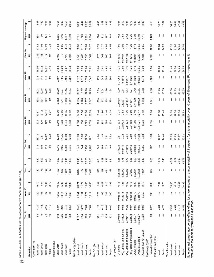
82
Yea
r 5
Yea
r 10
Yea
r 15
Yea
r 20
Yea
r 25
Yea
r 30
Yea
r 35
Yea
r 40
40-y
ear
aver
age
Ben
efits
RU
$R
U$
RU
$R
U$
RU
$R
U$
RU
$R
U$
RU
$
Coo
ling
(kW
h)
Yar
d: w
est
584.
3912
99.
7918
213
.82
213
16.1
323
317
.67
238
18.0
823
818
.06
235
17.8
219
114
.47
Yar
d: s
outh
191.
4651
3.84
795.
9710
37.
8112
09.
1213
410
.15
141
10.7
214
611
.06
997.
52
Yar
d: e
ast
342.
6082
6.24
120
9.11
144
10.8
915
912
.11
168
12.7
617
113
.01
172
13.0
413
19.
97
Pub
lic16
1.19
362.
7053
4.01
695.
2280
6.07
896.
7594
7.13
977.
3467
5.05
Hea
ting
(kB
tu)
Yar
d: w
est
518
5.07
1,06
310
.42
1,49
314
.63
1,81
617
.80
2,04
019
.99
2,15
221
.09
2,19
721
.53
2,19
821
.54
1,68
516
.51
Yar
d: s
outh
−22
6−
2.22
−51
7−
5.06
−63
3−
6.20
−48
5−
4.75
−36
3−
3.56
−21
1−
2.07
−95
−0.
935
0.05
−31
6−
3.09
Yar
d: e
ast
449
4.40
956
9.37
1,37
113
.44
1,70
316
.69
1,93
418
.95
2,05
620
.15
2,10
920
.67
2,12
020
.78
1,58
715
.56
Pub
lic66
36.
501,
363
13.3
61,
898
18.6
02,
275
22.3
02,
533
24.8
22,
657
26.0
42,
702
26.4
82,
697
26.4
32,
099
20.5
7
Net
ene
rgy
(kB
tu)
Yar
d: w
est
1,09
79.
472,
354
20.2
13,
314
28.4
53,
941
33.9
34,
368
37.6
64,
535
39.1
74,
577
39.5
94,
546
39.3
63,
591
30.9
8
Yar
d: s
outh
−34
−0.
76−
11−
1.22
154
−0.
2354
43.
0683
85.
561,
126
8.07
1,31
89.
791,
463
11.1
267
54.
42
Yar
d: e
ast
793
7.01
1,77
715
.60
2,57
222
.55
3,13
827
.58
3,52
931
.06
3,73
732
.90
3,82
433
.68
3,83
833
.81
2,90
125
.53
Pub
lic82
07.
691,
719
16.0
62,
427
22.6
12,
962
27.5
13,
333
30.8
93,
547
32.7
93,
642
33.6
13,
664
33.7
72,
764
25.6
2
Net
CO
2 (lb
)
Yar
d: w
est
171
1.28
375
2.81
535
4.01
645
4.84
725
5.44
758
5.69
773
5.80
770
5.78
594
4.46
Yar
d: s
outh
220.
1663
0.47
119
0.89
199
1.49
261
1.96
312
2.34
348
2.61
369
2.77
212
1.59
Yar
d: e
ast
125
0.94
287
2.15
421
3.16
521
3.91
595
4.46
634
4.76
656
4.92
660
4.95
487
3.66
Pub
lic12
10.
9026
01.
9537
52.
8146
93.
5253
84.
0357
84.
3460
14.
5160
74.
5644
43.
33
Air
pollu
tion
(lb)*
O3
upta
ke0.
0079
50.
030.
0398
40.
130.
0834
50.
280.
1522
50.
510.
2123
30.
710.
2979
51.
000.
3706
91.
240.
4493
91.
500.
20.
67
NO
2 up
take
and
avo
ided
0.15
822
0.53
0.36
318
1.21
0.53
272
1.78
0.66
411
2.22
0.75
738
2.53
0.82
001
2.74
0.85
422.
860.
8745
72.
920.
632.
10
SO
2 up
take
and
avo
ided
0.10
847
0.22
0.25
468
0.52
0.37
249
0.77
0.45
546
0.94
0.51
324
1.06
0.54
813
1.13
0.56
477
1.16
0.57
186
1.18
0.42
0.87
PM
10 u
ptak
e an
d av
oide
d0.
0247
80.
070.
0651
10.
180.
1217
0.35
0.20
712
0.59
0.31
488
0.89
0.43
811
1.24
0.44
121
1.25
0.44
212
1.26
0.26
0.73
VO
Cs
avoi
ded
0.02
277
0.09
0.05
272
0.20
0.07
681
0.29
0.09
383
0.35
0.10
560.
400.
1122
90.
420.
1152
30.
430.
1160
70.
440.
090.
33
BV
OC
s re
leas
ed−
0.00
027
0.00
−0.
0197
9−
0.07
−0.
0965
5−
0.36
−0.
2875
−1.
08−
0.57
971
−2.
17−
0.97
32−
3.65
−0.
9732
−3.
65−
0.97
32−
3.65
−0.
49-1
.83
Avo
ided
and
net
upt
ake
0.32
20.
930.
756
2.18
1.09
13.
101.
285
3.53
1.32
43.
421.
243
2.88
1.37
33.
301.
481
3.65
1.11
2.87
Hyd
rolo
gy (
gal)*
Rai
nfal
l int
erce
ptio
n59
0.27
196
0.90
394
1.81
767
3.53
1,09
55.
041,
671
7.68
2,16
09.
942,
690
12.3
81,
129
5.19
Est
hetic
s an
d ot
her
Yar
d--
-4.
01--
-7.
84--
-10
.52
---
12.2
2--
-13
.08
---
13.2
5--
-12
.86
---
12.0
4--
-10
.73
Pub
lic--
-4.
73--
-9.
26--
-12
.43
---
14.4
4--
-15
.45
---
15.6
5--
-15
.19
---
14.2
3--
-12
.67
Tota
l ben
efits
Yar
d: w
est
---
15.9
7--
-33
.95
---
47.8
9--
-58
.05
---
64.6
3--
-68
.68
---
71.4
8--
-73
.20
---
54.2
3
Yar
d: s
outh
---
4.62
---
10.1
7--
-16
.09
---
23.8
3--
-29
.05
---
34.2
3--
-38
.50
---
41.9
5--
-24
.81
Yar
d: e
ast
---
13.1
6--
-28
.68
---
41.1
4--
-50
.77
---
57.0
5--
-61
.48
---
64.6
9--
-66
.83
---
47.9
7
Pub
lic--
-14
.53
---
30.3
6--
-42
.77
---
52.5
2--
-58
.83
---
63.3
5--
-66
.55
---
68.5
8--
-49
.69
Tabl
e B
4—A
nnua
l ben
efits
for
the
repr
esen
tativ
e m
ediu
m tr
ee (
red
oak)
Not
e: A
nnua
l val
ues
inco
rpor
ate
effe
cts
of tr
ee lo
ss. W
e as
sum
e an
ann
ual m
orta
lity
of 1
per
cent
, for
a to
tal m
orta
lity
over
40
year
s of
40
perc
ent.
RU
= r
esou
rce
unit.
*Val
ues
are
the
sam
e fo
r ya
rd a
nd p
ublic
tree
s.

83
Co
sts
Yea
r 5
Yea
r 10
Yea
r 15
Yea
r 20
Yea
r 25
Yea
r 30
Yea
r 35
Yea
r 40
40-y
ear
aver
age
Tre
e an
d pl
antin
g
Yar
d80
.00
0.00
0.00
0.00
0.00
0.00
0.00
0.00
10.0
0
Pub
lic40
.00
0.00
0.00
0.00
0.00
0.00
0.00
0.00
5.00
Pru
ning
Yar
d0.
174.
324.
086.
866.
436.
005.
575.
144.
57
Pub
lic11
.88
22.5
021
.25
24.0
022
.50
21.0
019
.50
18.0
020
.11
Rem
ove
and
disp
ose
Yar
d1.
472.
733.
915.
026.
057.
017.
898.
704.
92
Pub
lic1.
102.
042.
933.
764.
545.
255.
926.
523.
71
Pes
t and
dis
ease
Yar
d0.
340.
590.
800.
971.
101.
191.
241.
260.
88
Pub
lic0.
030.
040.
060.
070.
080.
090.
090.
100.
07
Infr
astr
uctu
re r
epai
r
Yar
d0.
080.
150.
200.
240.
270.
300.
310.
320.
22
Pub
lic0.
420.
741.
001.
211.
371.
481.
551.
581.
10
Irrig
atio
n
Yar
d0.
380.
000.
000.
000.
000.
000.
000.
000.
05
Pub
lic0.
380.
000.
000.
000.
000.
000.
000.
000.
05
Cle
anup
Yar
d0.
000.
010.
010.
010.
010.
010.
010.
010.
01
Pub
lic0.
020.
030.
040.
040.
050.
050.
060.
060.
04
Liab
ility
and
lega
l
Yar
d0.
010.
020.
020.
020.
020.
020.
020.
020.
02
Pub
lic0.
060.
080.
090.
100.
100.
100.
090.
090.
09
Adm
inis
trat
ion
and
othe
r
Yar
d0.
000.
000.
000.
000.
000.
000.
000.
000.
00
Pub
lic1.
332.
333.
163.
824.
324.
674.
884.
973.
45
Tota
l cos
ts
Yar
d82
.46
7.81
9.02
13.1
113
.88
14.5
215
.04
15.4
520
.66
Pub
lic55
.21
27.7
728
.53
33.0
132
.95
32.6
432
.09
31.3
133
.61
Tabl
e B
5—A
nnua
l cos
ts fo
r th
e re
pres
enta
tive
med
ium
tree
(re
d oa
k)
Not
e: A
nnua
l val
ues
inco
rpor
ate
effe
cts
of tr
ee lo
ss. W
e as
sum
e an
ann
ual m
orta
lity
of 1
per
cent
, for
a to
tal m
orta
lity
over
40
year
s of
40
perc
ent.
*Alth
ough
tree
and
pla
ntin
g co
sts
occu
r in
yea
r 1,
this
val
ue w
as d
ivid
ed b
y 5
year
s to
der
ive
an a
vera
ge a
nnua
l cos
t for
the
first
5-y
ear
perio
d.
Tabl
e B
6—A
nnua
l net
ben
efits
for
the
repr
esen
tativ
e m
eidu
m tr
ee (
red
oak)
Not
e: A
nnua
l val
ues
inco
rpor
ate
effe
cts
of tr
ee lo
ss. W
e as
sum
e an
ann
ual m
orta
lity
of 1
per
cent
, for
a to
tal m
orta
lity
over
40
year
s of
40
perc
ent.
See
tabl
es B
4 fo
r an
nual
be
nefit
s an
d ta
ble
B5
for
annu
al c
osts
.
Net
ben
efits
Yea
r 5
Yea
r 10
Yea
r 15
Yea
r 20
Yea
r 25
Yea
r 30
Yea
r 35
Yea
r 40
40-y
ear
aver
age
Yar
d: w
est
−66
2639
4551
5456
5834
Yar
d: s
outh
−78
27
1115
2023
274
Yar
d: e
ast
−69
2132
3843
4750
5127
Pub
lic−
413
1420
2631
3437
16

84
Yea
r 5
Yea
r 10
Yea
r 15
Yea
r 20
Yea
r 25
Yea
r 30
Yea
r 35
Yea
r 40
40-y
ear
aver
age
Ben
efits
RU
$R
U$
RU
$R
U$
RU
$R
U$
RU
$R
U$
RU
$
Coo
ling
(kW
h)
Yar
d: w
est
745.
61
188
14.3
0 25
419
.29
301
22.8
2 32
324
.51
333
25.2
6 33
425
.36
333
25.2
6 26
820
.30
Yar
d: s
outh
302.
25
846.
35
140
10.6
3 19
114
.49
233
17.6
6 26
319
.98
283
21.4
9 29
222
.15
189
14.3
8
Yar
d: e
ast
473.
60
124
9.38
18
113
.71
224
17.0
2 25
018
.98
267
20.2
4 27
520
.90
280
21.2
2 20
615
.63
Pub
lic26
1.99
64
4.85
10
37.
85
137
10.3
7 16
112
.22
184
13.9
5 20
115
.22
212
16.0
6 13
610
.31
Hea
ting
(kB
tu)
Yar
d: w
est
938
9.19
19
8719
.47
2778
27.2
2 34
0033
.32
3796
37.2
0 40
2839
.48
4136
40.5
4 41
0540
.23
3146
30.8
3
Yar
d: s
outh
498
4.88
88
58.
67
1464
14.3
5 20
3219
.91
2555
25.0
4 29
5528
.96
3227
31.6
2 33
3632
.70
2119
20.7
7
Yar
d: e
ast
871
8.53
18
5818
.21
2663
26.0
9 33
1032
.44
3742
36.6
7 40
0239
.22
4131
40.4
9 41
0740
.25
3085
30.2
4
Pub
lic10
4110
.20
2235
21.9
1 30
9630
.34
3756
36.8
1 41
4940
.66
4357
42.6
9 44
3443
.45
4373
42.8
5 34
3033
.61
Net
ene
rgy
(kB
tu)
Yar
d: w
est
1678
14.8
0 38
7233
.78
5319
46.5
1 64
0756
.14
7026
61.7
1 73
5764
.74
7478
65.9
0 74
3465
.49
5821
51.1
3
Yar
d: s
outh
795
7.13
17
2115
.02
2865
24.9
8 39
4134
.40
4882
42.7
0 55
8848
.94
6059
53.1
2 62
5454
.84
4013
35.1
4
Yar
d: e
ast
1345
12.1
3 30
9427
.59
4470
39.8
1 55
5249
.46
6243
55.6
5 66
6959
.46
6885
61.3
9 69
0461
.47
5145
45.8
7
Pub
lic13
0312
.19
2875
26.7
6 41
3038
.19
5122
47.1
8 57
6052
.89
6195
56.6
4 64
3958
.67
6488
58.9
1 47
8943
.93
Net
CO
2 (lb
)
Yar
d: w
est
242
1.81
56
84.
26
798
5.98
97
97.
34
1097
8.22
11
718.
78
1213
9.10
12
259.
19
911
6.84
Yar
d: s
outh
119
0.89
27
12.
03
460
3.45
64
24.
82
806
6.04
93
37.
00
1024
7.68
10
698.
02
665
4.99
Yar
d: e
ast
191
1.43
44
93.
37
666
5.00
84
66.
34
973
7.30
10
627.
96
1118
8.39
11
408.
55
806
6.04
Pub
lic17
71.
33
398
2.98
59
34.
45
758
5.68
87
86.
59
970
7.28
10
347.
75
1062
7.96
73
45.
50
Air
pollu
tion
(lb)*
O3
upta
ke0.
0071
0.02
0.
0330
50.
11
0.09
675
0.32
0.
1795
20.
60
0.28
223
0.94
0.
4152
91.
39
0.54
892
1.84
0.
7161
62.
39
0.28
0.95
NO
2 up
take
and
avo
ided
0.25
532
0.85
0.
6210
42.
08
0.91
762
3.07
1.
1615
53.
88
1.33
272
4.46
1.
4597
74.
88
1.54
222
5.16
1.
5925
5.32
1.
113.
71
SO
2 up
take
and
avo
ided
0.15
124
0.31
0.
3927
60.
81
0.58
165
1.20
0.
7336
51.
51
0.83
551
1.72
0.
9093
61.
87
0.95
51.
97
0.98
166
2.02
0.
691.
43
PM
10 u
ptak
e an
d av
oide
d0.
0362
50.
10
0.09
596
0.27
0.
1604
60.
46
0.25
102
0.71
0.
3586
31.
02
0.48
471.
38
0.63
589
1.81
0.
8077
22.
29
0.35
1.01
VO
Cs
avoi
ded
0.03
362
0.13
0.
0849
0.32
0.
1249
0.47
0.
1568
90.
59
0.17
802
0.67
0.
1926
10.
72
0.20
106
0.75
0.
2047
70.
77
0.15
0.55
BV
OC
s re
leas
ed0
0.00
0
0.00
0
0.00
0
0.00
0
0.00
0
0.00
0
0.00
0
0.00
0
0.00
Avo
ided
and
net
upt
ake
0.48
41.
42
1.22
83.
59
1.88
15.
51
2.48
37.
30
2.98
78.
81
3.46
210
.24
3.88
311
.52
4.30
312
.80
2.59
7.65
Hyd
rolo
gy (
gal)*
Rai
nfal
l int
erce
ptio
n13
30.
61
374
1.72
80
73.
71
1,39
46.
41
2,14
69.
87
3,07
114
.13
3,98
718
.34
5387
24.7
8 21
629.
95
Est
hetic
s an
d ot
her
Yar
d--
-9.
07
---
15.7
2 --
-20
.93
---
24.8
5 --
-27
.59
---
29.2
9 --
-30
.06
---
30.0
2 --
-23
.44
Pub
lic--
-10
.71
---
18.5
7 --
-24
.73
---
29.3
6 --
-32
.60
---
34.6
0 --
-35
.51
---
35.4
7 --
-27
.69
Tota
l ben
efits
Yar
d: w
est
---
27.7
1 --
-59
.06
---
82.6
5 --
-10
2.04
--
-11
6.21
--
-12
7.17
--
-13
4.91
--
-14
2.28
--
-99
.01
Yar
d: s
outh
---
19.1
2 --
-38
.07
---
58.5
9 --
-77
.77
---
95.0
1 --
-10
9.59
--
-12
0.72
--
-13
0.46
--
-81
.17
Yar
d: e
ast
---
24.6
6 --
-51
.98
---
74.9
6 --
-94
.36
---
109.
22
---
121.
08
---
129.
69
---
137.
63
---
92.9
5
Pub
lic--
-26
.26
---
53.6
2 --
-76
.60
---
95.9
3 --
-11
0.76
--
-12
2.89
--
-13
1.79
--
-13
9.93
--
-94
.72
Not
e: A
nnua
l val
ues
inco
rpor
ate
effe
cts
of tr
ee lo
ss. W
e as
sum
e an
ann
ual m
orta
lity
of 1
per
cent
, for
a to
tal m
orta
lity
over
40
year
s of
40
perc
ent.
RU
= r
esou
rce
unit.
*Val
ues
are
the
sam
e fo
r ya
rd a
nd p
ublic
tree
s.
Tabl
e B
7—A
nnua
l ben
efits
for
the
repr
esen
tativ
e la
rge
tree
(ha
ckbe
rry)

85
Co
sts
Yea
r 5
Yea
r 10
Yea
r 15
Yea
r 20
Yea
r 25
Yea
r 30
Yea
r 35
Yea
r 40
40-y
ear
aver
age
Tre
e an
d pl
antin
g*
Yar
d80
.00
0.00
0.00
0.00
0.00
0.00
0.00
0.00
10.0
0
Pub
lic40
.00
0.00
0.00
0.00
0.00
0.00
0.00
0.00
5.00
Pru
ning
Yar
d0.
344.
324.
086.
866.
436.
005.
575.
144.
96
Pub
lic11
.88
22.5
021
.25
24.0
022
.50
21.0
019
.50
18.0
020
.61
Rem
ove
and
disp
ose
Yar
d2.
023.
605.
146.
628.
059.
4410
.77
12.0
56.
59
Pub
lic1.
512.
703.
854.
976.
047.
088.
089.
044.
96
Pes
t and
dis
ease
Yar
d0.
460.
781.
061.
281.
461.
601.
691.
751.
18
Pub
lic0.
040.
060.
080.
100.
110.
120.
130.
130.
09
Infr
astr
uctu
re r
epai
r
Yar
d0.
120.
200.
260.
320.
370.
400.
420.
440.
30
Pub
lic0.
580.
981.
321.
601.
832.
002.
122.
191.
48
Irrig
atio
n
Yar
d0.
380.
000.
000.
000.
000.
000.
000.
000.
05
Pub
lic0.
380.
000.
000.
000.
000.
000.
000.
000.
05
Cle
anup
Yar
d0.
000.
010.
010.
010.
010.
010.
020.
020.
01
Pub
lic0.
020.
040.
050.
060.
070.
070.
080.
080.
05
Liab
ility
and
lega
l
Yar
d0.
010.
020.
020.
020.
020.
020.
030.
020.
02
Pub
lic0.
060.
080.
100.
110.
120.
120.
130.
120.
10
Adm
inis
trat
ion
and
othe
r
Yar
d0.
000.
000.
000.
000.
000.
000.
000.
000.
00
Pub
lic1.
833.
094.
165.
045.
756.
296.
666.
884.
65
Tota
l cos
ts
Yar
d83
.33
8.93
10.5
715
.11
16.3
417
.47
18.4
919
.42
23.1
0
Pub
lic56
.29
29.4
530
.81
35.8
736
.41
36.6
836
.68
36.4
436
.99
Tabl
e B
8—A
nnua
l cos
ts fo
r th
e re
pres
enta
tive
larg
e tr
ee (
hack
berr
y)
Not
e: A
nnua
l val
ues
inco
rpor
ate
effe
cts
of tr
ee lo
ss. W
e as
sum
e an
ann
ual m
orta
lity
of 1
per
cent
, for
a to
tal m
orta
lity
over
40
year
s of
40
perc
ent.
*Alth
ough
tree
and
pla
ntin
g co
sts
occu
r in
yea
r 1,
this
val
ue w
as d
ivid
ed b
y 5
year
s to
der
ive
an a
vera
ge a
nnua
l cos
t for
the
first
5-y
ear
perio
d.
Tabl
e B
9—A
nnua
l net
ben
efits
for
the
repr
esen
tativ
e la
rge
tree
(ha
ckbe
rry)
Not
e: A
nnua
l val
ues
inco
rpor
ate
effe
cts
of tr
ee lo
ss. W
e as
sum
e an
ann
ual m
orta
lity
of 1
per
cent
, for
a to
tal m
orta
lity
over
40
year
s of
40
perc
ent.
See
tabl
es B
7 fo
r an
nual
be
nefit
s an
d ta
ble
B8
for
annu
al c
osts
.
Net
ben
efits
Yea
r 5
Yea
r 10
Yea
r 15
Yea
r 20
Yea
r 25
Yea
r 30
Yea
r 35
Yea
r 40
40-y
ear
aver
age
Yar
d: w
est
−56
5072
8710
011
011
612
376
Yar
d: s
outh
−64
2948
6379
9210
211
158
Yar
d: e
ast
−59
4364
7993
104
111
118
70
Pub
lic−
3024
4660
7486
9510
358


Pacific Southwest Research Station
PO Box 245
Berkeley, CA 94701
www.fs.fed.us/psw

USDA Forest Service, Pacific Southwest Research StationCenter for Urban Forest Research One Shields Avenue, UC Davis, Davis, California 95616(530) 752-7636 Fax (530) 752-6634 http://www.fs.fed.us/psw/programs/cufr/