Midweek intensification of rain in the U.S.: Does air … · weekly cycle in summertime rainfall...
18
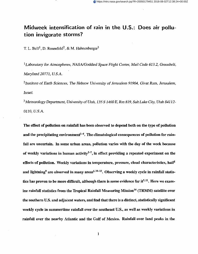
Midweek intensification of rain in the U.S.: Does air pollu- tion invigorate storms? T. L. Bell', D. Rosenfeld2, & M. Hahnenberge2 Laboratory for Atmospheres, NASNGoddard Space Flight Center, Mail Code 61 3.2, Greenbelt, Maryland 20771, U.S.A. 21nstitute of Earth Sciences, The Hebrew University of Jerusalem 91904, Givat Ram, Jerusalem, Israel. Meteorology Department, University of Utah, 135 S 1460 E, Rm 819, Salt Lake City, Utah 841 12- 01 10, U.S.A. The effect of pollution on rainfall has been observed to depend both on the type of pollution and the precipitating environment1-". The climatological consequences of pollution for rain- fall are uncertain. In some urban areas, pollution varies with the day of the week because of weekly variations in human activity5-', in effect providing a repeated experiment on the effects of pollution. Weekly variations in temperature, pressure, cloud characteristics, hails and lightning9are observed in many Observing a weekly cycle in rainfall statis- tics has proven to be more difficult, although there is some evidence for it5911. Here we exam- ine rainfall statistics from the Tropical Rainfall Measuring Mission14 (TRMM) satellite over the southern U.S. and adjacent waters, and find that there is a distinct, statistically significant weekly cycle in summertime rainfall over the southeast U.S., as well as weekly variations in rainfall over the nearby Atlantic and the Gulf of Mexico. Rainfall over land peaks in the 1 https://ntrs.nasa.gov/search.jsp?R=20050179451 2018-08-02T12:38:24+00:00Z
Transcript of Midweek intensification of rain in the U.S.: Does air … · weekly cycle in summertime rainfall...
Midweek intensification of rain in the U.S.: Does air pollu- tion invigorate storms?
T. L. Bell', D. Rosenfeld2, & M. Hahnenberge2
Laboratory for Atmospheres, NASNGoddard Space Flight Center, Mail Code 61 3.2, Greenbelt,
Maryland 20771, U.S.A.
21nstitute of Earth Sciences, The Hebrew University of Jerusalem 91 904, Givat Ram, Jerusalem,
Israel.
Meteorology Department, University of Utah, 135 S 1460 E, Rm 819, Salt Lake City, Utah 841 12-
01 10, U.S.A.
The effect of pollution on rainfall has been observed to depend both on the type of pollution
and the precipitating environment1-". The climatological consequences of pollution for rain-
fall are uncertain. In some urban areas, pollution varies with the day of the week because
of weekly variations in human activity5-', in effect providing a repeated experiment on the
effects of pollution. Weekly variations in temperature, pressure, cloud characteristics, hails
and lightning9 are observed in many Observing a weekly cycle in rainfall statis-
tics has proven to be more difficult, although there is some evidence for it5911. Here we exam-
ine rainfall statistics from the Tropical Rainfall Measuring Mission14 (TRMM) satellite over
the southern U.S. and adjacent waters, and find that there is a distinct, statistically significant
weekly cycle in summertime rainfall over the southeast U.S., as well as weekly variations in
rainfall over the nearby Atlantic and the Gulf of Mexico. Rainfall over land peaks in the
1
https://ntrs.nasa.gov/search.jsp?R=20050179451 2018-08-02T12:38:24+00:00Z

middle of the week, suggesting that summer rainfall on large scales may increase as pollution
levels rise. Both rain statistics over land and what appear to be compensating effects over
adjacent seas support the suggestion that air pollution invigorates convection and outflow
aloft.
Pollution aerosols have been documented to suppress precipitation from shallow clouds
(cloud heights below about the -10°C isotherm)'i2* l5-I7. When polluted clouds develop to greater
heights (lower temperatures), however, as often happens in the summertime over land, it has been
suggested'*, l9 that suppressed rainout enables unprecipitated water to reach greater heights where
freezing can release latent heat and further invigorate the cloud updrafts. This might in turn de-
lay the onset of precipitation and the development of downdrafts and so prolong the growth of the
convective cloud, allowing more water vapor to be ingested and further invigoration of the st01-m'~.
Recent cloud simulations2' support this suggestion: in a moist, unstable atmosphere such as pre-
vails during the summer in the SE U.S., pollution aerosols can induce clouds to develop stronger
updrafts and downdrafts, grow taller, trigger secondary storm development, and produce more rain.
The analyses of weekly cycles in satellite precipitation estimates reported here might serve as the
first observational evidence of this suggestion, and provide a first clue towards quantifying it on a
climate scale.
It is well d ~ c u m e n t e d ~ ~ ~ , ' ~ ~ ~ ~ ~ ~ ~ that pollution levels change with the day of the week in
many urban areas, generally attributed to changes in vehicular traffic, though variations in power
consumption may also play a role. Searches for a weekly cycle in precipitation have yielded mixed
2

r e ~ u l t s ~ ~ * ~ ~ * ~ ~ ~ ~ . Our results suggest in fact that the weekly cycle is weaker in coastal areas, and
studies of data from coastal cities may therefore have failed to find a significant weekly cycle in
precipitation for this reason. Cerveny & Balling" ("CB" hereafter), using rain estimates from the
Microwave Sounding Unit (MSU) on TIROS-N satellites25 for 1979-1995 found a weekly cycle
in precipitation over the Atlantic near the east coast of the U.S., with peak rainfall occurring on
Saturday and minimum rainfall on Monday.
The TRMM satellite has been orbiting the Earth since late 1997. It is unique in that it carries
a meteorological radar which can be used to improve the rain estimates made with its passive
microwave instrument, the TRMM Microwave Imager (TMI). Averages for each day of the week
based on 6 years (1998-2003) of data for summertime (June-August) rain rates, estimated using
version 5 of the TMI retrieval were obtained for each 2.5" x 2.5" grid box viewed by
TRMM in the vicinity of the continental U.S. (TRMM's orbital plane is inclined 35" with respect
to the Equator, and the TMI cannot see poleward of 40°.)
The daily averages r ( t ) were fit to a sinusoidal form
with w-/ = 2n/(7d), t the day of the week, ro the average rain rate, r7 the amplitude of the weekly
cycle, and @7 the day of the week when the sinusoidal fit peaks. The statistical significance of the
amplitude q relative to the hypothesis that there is no weekly cycle (1-7 = 0) was obtained using a
technique based on the one described by Bell & Reid27. Figure l a shows a map of the phase for
each grid box, with gray level adjusted according to the significance level of the weekly amplitude.
3
The strongest colors indicate significance levels at p = 0.05 ("2-sigma") or better. Although there
is considerable variability in the phase (much of which can be explained by sampling error due to
the length of the dataset), it appears that there is a tendency for average rain rates to peak during
the middle of the week (Tue-Thu) over the continental U.S., and to peak Sat-Mon over the nearby
Atlantic and perhaps the Gulf of Mexico. There also appears to be a tendency for the weekly cycle
to weaken near the coasts. (We note that weekly variations in hail intensity have been observed to
weaken as one approaches the Atlantic coast of France from inland8.)
Even with 6 years of data, the statistical uncertainty in the weekly cycle in many of the grid
boxes is large. We therefore try to increase the signal-to-noise ratio by averaging over larger areas,
guided by our physical understanding of where and how the weekly cycle in pollution is likely to
affect precipitation. Summer precipitation over the U.S. differs markedly in the eastern and western
halves, due in part to the effects of the moisture brought to the eastern half from the Gulf of Mexico
by prevailing winds and in part to the differences in topography. We have therefore derived average
rain rates from the five averaging areas A-E shown in Fig. lb. Grid boxes containing substantial
amounts of coastline are excluded. Area C is identical to the region examined by CB except for
two 2.5" grid boxes in their area too far north for TRMM.
Figure 2a shows the average rain rate for each day of the week for areas A-C. The SE U.S.
(area B) average daily rain rate for Tue-Fri is higher than for Sat-Mon, with a maximum on Tue.
The SW U.S. (area A) seems to show a weak cycle with slightly higher rates during weekdays
compared with weekends. In contrast, the coastal Atlantic (area C) shows strongest rain rates
4

Sat-Mon and lower rain rates Tue-Fri, similar to what CB found, but it should be noted that they
averaged data over entire years whereas our average includes only summers. Figure 3a shows the
average rain rate for areas C-E. The Atlantic region D east of region C seems to show a weaker but
similar cycle. The Gulf of Mexico area E has a mild cycle with largest values Fri-Sun and smallest
values Mon-Thu.
Figures 2b and 3b show the daily average fraction of TMI footprints (nominally of order
10 km in diameter) with detectable rain in them. It appears that the weekly cycle over the SE
U.S. is due as much to intensification of rain rates as to an increase in the area or frequency with
which it rains, whereas over the other areas the weekly response is more due to changes in area
or frequency than to intensification. This is brought out further in Figs. 2c and 3c, where the ratio
of the mean rain rate (panel a) to mean fraction-with-rain (panel b) is plotted. Note the increase
in intensity over the SE U.S. in Fig. 2c during midweek (although the minimum on Friday is not
readily explained).
The question immediately arises concerning whether these cycles are artifacts of the obser-
vational characteristics of TRMM, or accidents due to natural variability of precipitation unrelated
to the day of the week. In Methods we discuss why the sampling pattern of TRMM is unlikely to
have generated spurious weekly cycles of the magnitude seen here. Bootstrap techniques used to
estimate the statistical signficance of the cycles are also described there.
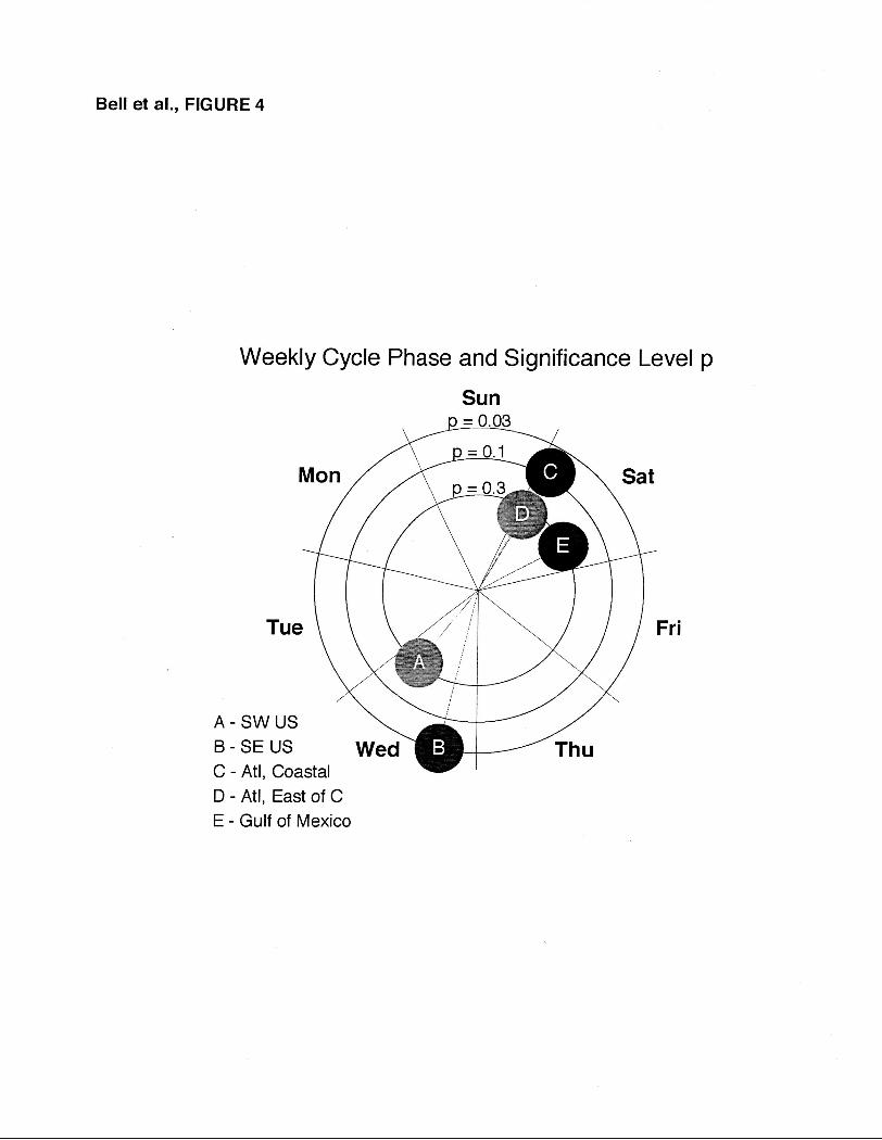
Figure 4 shows the phases and significance levels p for the averages over each of the 5 areas
in Fig. l b derived from fitting the 6 summers of TRMM data to the sinusoid (l), with p estimated
5
using the bootstrap approach described in Methods. Distance from the origin is proportional to
I/*. The weekly cycle of the average over the SE U.S. (area B) is significant at the p = 0.03
level [ro = 0.180 mmh-’, 1-7 = 0.042 mmh-’, 9/ = 4.7d (& = 0 .--) 0000 Saturday)]. The coastal
Atlantic (area C) cycle is significant at the p = 0.08 level [ro = 0.266 mmh-’, 7-7 = 0.054 mmh-’;
&I = 0.9dI. The other 3 area averages have weekly amplitudes that are approximately “1-sigma”
in size, and so are not very well determined by the amount of data analyzed; by themselves they
would not constitute much “proof” of a weekly cycle, but if one accepts that there is a weekly
cycle in these last three area averages, there is some information to be gleaned.
The SE U.S. area B appears to have a significant weekly cycle; its amplitude is almost 25%
of the mean. The plot in Fig. 2a indicates that average rain rate over the SE U.S. is largest during
the middle of the week and drops to its lowest value on Sunday-behavior very similar to anthro-
pogenic pollution. This suggests that summertime (mostly convective) rain amounts are increased,
at least on large scales, by the increase in the lunds of pollution that vary weekly because of hu-
man activity. Figs. 2b,c suggest that the increase is due in about equal parts to intensification and
increase in aredfrequency. It is important at this point, however, to recall how the TMI is used to
obtain rain-rate estimates. Over land the estimates are based mostly on microwave radiance mea-
sured by the 85 GHz channel, which responds chiefly to the amount and size of ice particles at the
tops of clouds. Since production of ice aloft is common during the intense convection in summer
storms, this method of estimating rainfall at the surface generally works quite However,
clouds with smaller drops such as caused by air pollution have been documented to produce larger
raindrops for the same rain intensities, mainly due to the larger ice hydrometeors aloft2*. The
6

pollution-induced invigoration of the clouds also produces larger ice hydrometeors aloft2'. There-
fore it is possible that the weekly cycle in the TRMM rain estimates may be due to changes in the
ice aloft that are not in fact accompanied by much change in rainfall at the surface. The dynami-
cal implications of such changes in cloud structure would be important, however, even if surface
rainfall were to be unaffected.
The weaker response over the SW U.S. (area A) is consistent with simulations showing that
invigoration of convection by pollution is diminished in drier conditions, and may even reverse2'.
The weekly cycle in the Atlantic off the east coast of the U.S. (area C) is remarkable in that
it is almost exactly opposite in phase to the cycle over the nearby land. Several explanations are
possible:
1) the effect of pollution on rain formation over the ocean may be quite different from its
effect on the more vigorous convection over land;
2) the phase difference may be due to the lag in time when pollution is carried to this region
from the land;
3) precipitation over the ocean may be dynamically suppressed when it is most vigorous over
the nearby continent.
Explanation 1 is plausible, given that convection is less vigorous and less ice is formed over
the ocean, and sea salt aerosols mitigate some of the suppression effects of the pollution aerosol^'^.
Explanation 2 was offered by CB, who mention that they saw a steadily increasing delay in peak
rainfall in the oceanic areas further and further east of area C. The almost simultaneous peak in
7

the rainfall over area D (Fig. 3) does not seem to be consistent with this hypothesis, however. (We
examined the rainfall over an area east of D and adjacent to it, which has a slight weekly cycle,
but its phase is not statistically distinguishable from that of the two oceanic areas C and D.) Expla-
nation 3 is consistent with invigoration of the convection over land, which must be compensated
somewhere with downward motion of the air. It involves quantitative dynamical understanding of
how changes in convection over the continent might affect offshore convection, and will probably
require modeling studies to evaluate it.
Methods
Because TRMM visits a grid box several days in a row at the same hour (local time) of the day,
then visits the box for several days one hour earlier (local time), et^.^^, there is some danger that the
satellite might, for example, consistently overfly an area on weekends at noontime while visiting
the area during the middle of the week only at night. In other words, the diurnal variation of
rainfall might produce an artificial weekly cycle in the TRMM observations. This possibility has
been ruled out by examining the number of observations as a function of both the day of the week
and the hour of the day: all hours of the day are about equally observed each day of the week. We
have also replaced the actual time series of area averages with an artificial diurnal cycle and found
that the spurious weekly cycle it generates is two orders of magnitude smaller than the observed
cycle.
The likelihood that the weekly cycle is an accident of natural variation in rainfall, which, of
course, has no preferred day of the week, has been estimated in two ways, both of which proved
8

to give similar values for the statistical significance level of the cycles: The first method is based
on a method described in [27], and involves estimating the sampling error in a sinusoidal fit to the
weekly cycle as in Eq. (1). The time series is broken into 2-week long chunks, each of which is fit
to the linear version of Eq. (1) with 3 unknown amplitudes, r(t) = ro + q c o s ( w t ) + s7sin(qt) .
The amplitude and phase q, & in (1) are derived from c7 and s7. The variance in the coefficients
c7 and s7 can then be used to estimate the error in the least squares estimates of r7, & from the
entire series. The second method uses a bootstrap (resampling) approach that generates artificial
(resampled) time series from randomly chosen chunks of data while attempting to preserve the time
correlation in the data30. (Most bootstrap studies use randomly chosen data points.) Resampling
was carried out by using the original time sequence of observations, dividing it into chunks of
lengths 4, 5, or 6 days (randomly chosen) and replacing each chunk with another segment of the
same length randomly selected from those segments of the data whose local times of observation
are within 2 hours of the chunk being replaced. This preserves the effects of the diurnal cycle of
rainfall in the statistics, but scrambles any associations with the day of the week. A set of 10,000
fake time series and the associated fits r p ) and a = 1,. . . , 10,000, were obtained. The
fraction of fits rp’ larger than the observed amplitude r7 for the actual data was used to estimate
the probability p that the observed amplitude was an accident, under the null hypothesis that there
is no real weekly cycle.
1. Rosenfeld, D. TRMM observed first direct evidence of smoke from forest fires inhibiting
rainfall. Geophys. Res. Lett. 26,3105-3108 (1999).
9

2. Rosenfeld, D. Suppression of rain and snow by urban and industrial air pollution. Science
287,1793-1796 (2000).
3. Phillips, V. T. J., Choularton, T. W., Blyth, A. M. & Latham, J. The influence of aerosol
concentrations on the glaciation and precipitation of a cumulus cloud. Quart. J. Roy. Meteox
SOC. 128,951-971 (2002).
4, Rudich, Y. & Khersonsky, 0. Treating clouds with a grain of salt. Geophys. Res. Lett. 29,
10.1029/2002GL016055 (2002).
5. Simmonds, I. & Keay, K. Weekly cycle of meteorological variations in Melbourne and the
role of pollution and anthropogenic heat release. Atmos. Environ. 31,1589-1603 (1997).
6. Marr, L. C. & Harley, R. A. Modeling the effect of weekday-weekend differences in motor
vehicle emissions on photochemical air pllution in central California. Environ. Sci. Technol.
36,4099-4106 (2002).
7. Beirle, S., Platt, U., Wenig, M. & Wagner, T. Weekly cycle of NO2 by GOME measurements:
A signature of anthropogenic sources. Atmos. Chem. Phys. 3,2225-2232 (2003).
8. Dessens, J., Fraile, R., Pont, V. & Sanchez, J. L. Day-of-the-week variability of hail in south-
western France. Atmos. Res. 59,63-76 (2001).
9. Mullayarov, V. A., Karimov, R. R., Kozlov, V. I. & Poddelsky, I. N. Possible weekly
variations in the thunderstorm activity. J. Atmos. Solar-Terx Phys. 67,397-403 (2005). URZ,
http://gateway.isiknowledge.com/gateway/Gateway.cgi?GWVersion=2&SrcAuth=
10
Alerting&SrcApp=Alerting&DestApp=WOS&DestLinkType=FullRecord;KeyUT=OOO22
7269700009.
10. Gordon, A. H. Weekdays warmer than weekends? Nature 367,325-326 (1994).
11. Cerveny, R. S. & Balling, R. C., Jr. Weekly cycles of air pollutants, precipitation and tropical
cyclones in the coastal NW Atlantic region. Nature 394,561-563 (1998).
12. de E Forster, P. M. & Solomon, S . Observations of a “weekend effect” in diurnal temperature
range. Proc. Nat. Acad. Sciences 100,11225-1 1230 (2003).
13. Jin, M., Shepherd, J. M. & King, M. D. Urban aerosols and their variations with clouds and
rainfall: A case study for New York and Houston. J. Geophys. Res. (2005). In press.
14. Kummerow, C. et al. The status of the Tropical Rainfall Measuring Mission (TRMM) after
two years in orbit. J. Appl. Meteor 39, 1965-1982 (2000).
15. Gunn, R. & Phillips, B. B. An experimental investigation of the effect of air pollution on the
initiation of rain. J. Meteol: 14,272-280 (1957).
16. Albrecht, B. A. Aerosols, cloud microphysics and fractional cloudiness. Science 245, 1227-
1230 (1989).
17. Rosenfeld, D., Lahav, R., Khain, A. P. & Pinsky, M. The role of sea-spray in cleansing air
pollution over ocean via cloud processes. Science 297,1667-1670 (2002).
18. Williams, E. et aE. Contrasting convective regimes over the Amazon: Implications for cloud
electrification. J. Geophys. Res. 107, 10.1029/2001JD000380 (2002).
11
19. Andreae, M. 0. et al. Smoking rain clouds over the Amazon. Science 303,1337-1342 (2004).
20. Khain, A., Rosenfeld, D. & Pokrovsky, A. Aerosol impact on the dynamics and microphysics
of convective clouds. Q. J. Royal Meteol: SOC. (2005). Submitted.
21. Salcedo, R. L. R., AlvimFerraz, M. C. M., Alves, C. A. & Martins, F. G. Time-series analysis
of air pollution data. Atmos. Envir 33,2361-2372 (1999).
22. Blanchard, C. L. & Tanenbaum, S . J. Differences between weekday and weekend air pollutant
levels in southern California. J. Air Waste Management Assoc. 53, 816-828 (2003).
23. Cehak, K. Note on the dependence of precipitation on the day of the week in a medium
industrialized city. Arch. Met. Geoph. Biokl. B30,247-25 1 (1982).
24. DeLisi, M. P. & Cope, A. M. Weekly precipitation cycles along the Northeast Corridor?
Weather and Forecasting 16,343-353 (2001).
25. Spencer, R. W. Global oceanic precipitation from the MSU during 1979-1991 and comparisons
with other climatologies. J. Clim. 6, 1301-1326 (1993).
26. Kummerow, C. et al. The evolution of the Goddard Profiling Algorithm (GPROF) for rainfall
estimation from passive microwave sensors. J. Appl. Meteor 40, 1801-1820 (2001).
27. Bell, T. L. & Reid, N. Detecting the diurnal cycle of rainfall using satellite observations. J.
Appl. Meteol: 32,3 11-322 (1993).
28. Rosenfeld, D. & Ulbrich, C. W. Cloud microphysical properties, processes, and rain-
fall estimation opportunities. In Wakimoto, R. M. & Srivastava, R. (eds.) Radar
12

and Atmospheric Science: A Collection of Essays in Honor of David Atlas, vol. 52
of Meteorological Monographs, chap. 10, 237-258 (Amer. Met. SOC., 2003). URL
http://earth.huji.ac.il/data/pics/ZR-Met-Monog.pdf.
29. Negri, A. J., Bell, T. L. & Xu, L. Sampling of the diurnal cycle of precipitation using TRMM.
J. Atmos. Oceanic Tech. 19, 1333-1344 (2002).
30. Wilks, D. S. Resampling hypothesis tests for autocorrelated fields. J. Climate 10, 65-82
(1 997).
Acknowledgements Research by TLB was supported by the Office of Earth Science of the National Aero-
nautics and Space Administration as part of the Precipitation Measurement Mission program. Special thanks
to P. K. Kundu and the Data Mining Effort at the Goddard Earth Sciences DAAC, especially J. M. McManus
and W. L. Teng, who greatly facilitated processing the data used in this study.
Competing Interests The authors declare that they have no competing financial interests.
Correspondence and requests for materials should be addressed to T.L.B. ([email protected]).
13

Figure 1 Study region and gridded phases of weekly cycle. a, Colors for each grid box indicate
day of the week with maximum rainfall, based on fits to a 7-d sinusoid of averages of TRMM
rain estimates for 6 summers. Grayness of colors is based on the significance level p for the
amplitude. Areas with rain rates less than 0.01 mmh-* are masked. b, Five averaging areas
chosen t o improve the signal-to-noise ratio for cycle detection.
Figure 2 Rain statistics from TRMM for each day of the week for areas A-C in Fig. l b . a,
Average rain rate. b, Fraction of TMI footprints with rain. c, Ratio of results in panels a and b,
indicating intensity of rain where it rains (i.e., conditional on R > 0).
Figure 3 Rain statistics as in Fig. 2 for areas C-E in Fig. l b . Statistics for area C in Fig. 2
repeated here to aid comparisons.
Figure 4 Phase and significance level of weekly cycles for 5 areas. Angular position is determined
by day of week with maximum rain rate in sinusoidal fits to plots in Figs. 2a and 3a, and radial
position is determined by significance level of weekly cycle.
14

Bell et al., FIGURE 1
Phase of Weekly Cycle (JJA) 40
30
20
p < 0.050 p > 0.500 fl R < 0.01 mm/h
40
30 :
Sat Sun Mon Tue Wed Thu Fri
Averaging Regions
20 i
.....
.....
.....

Bell et al., FIGURE 2
- Sat Sun Mon Tue Wed Thu Fri Sat Sun Mon Tue Wed Thu Fri
Sat Sun Mon Tue Wed Thu Fri Sat Sun Mon Tue WedThu Day of Week

Bell et al., FIGURE 3
- Sat Sun Mon Tue Wed Thu Fri Sat Sun Mon Tue Wed Thu Fri
n
2 4 a
Sat Sun Mon Tue Wed Thu 8 ‘t
Fri Sat Sun Mon Tue Wed Thu
A - Y
- Fri
Day of Week
Bell et al., FIGURE 4
A - B - C -
Weekly Cycle Phase and Significance Level p
Sun
Mon
Fri
sw us SE US We hu Atl, Coastal
D - Atl, East of C E - Gulf of Mexico