1

Microneedle Delivery of

Ophthalmic Macromolecules

Cherilyn Go

Alan Gomez

Brian Hsu

Hillary Lam

BENG 221

October 24, 2014

2

Table of Contents

Introduction............................................................................................................................... 3

Microneedle Model.................................................................................................................... 4

Topical Delivery Model............................................................................................................. 4

Results and Discussion of Microneedle Model........................................................................ 6

Limitations of Analytical and Numerical Methods................................................................ 8

Results and Discussion of Topical Delivery Model................................................................. 8

Model Limitations and Adjustments ....................................................................................... 10

Conclusion................................................................................................................................. 10

References.................................................................................................................................. 11

Appendix A: Analytical Solution ............................................................................................ 12

Appendix B: Matlab Code for Analytical Solution ............................................................... 14

Appendix C: Matlab Code for Numerical Methods .............................................................. 16

3

Introduction

Since the introduction of human insulin for the treatment of diabetes, the use of

biopharmaceuticals for the treatment of human disease and illness has rapidly increased [1].

Biopharmaceuticals allow for the treatment of diseases with few side effects whereas typical

pharmaceuticals may be less effective or exhibit harmful side effects. One major field of

medicine in which biomolecules have been making an impact is in the treatment of ocular

diseases. In 2010, the number of visually impaired people worldwide was approximately 285

million, of which 39 million people were blind [2]. The most common diseases that significantly

affect vision are age-related macular degeneration (AMD), diabetic retinopathy, cataracts,

uveitis, keratitis, and glaucoma [3]. There already exists a number of biomolecules for

ophthalmic indications approved by the FDA such as aptamer, pegatanib and ranibizumab [4],

with many more in clinical trials. As the sales of ophthalmic biopharmaceuticals are expected to

exceed $8 billion in 2016, there is a significant market for improvements in ophthalmic

treatments [4].

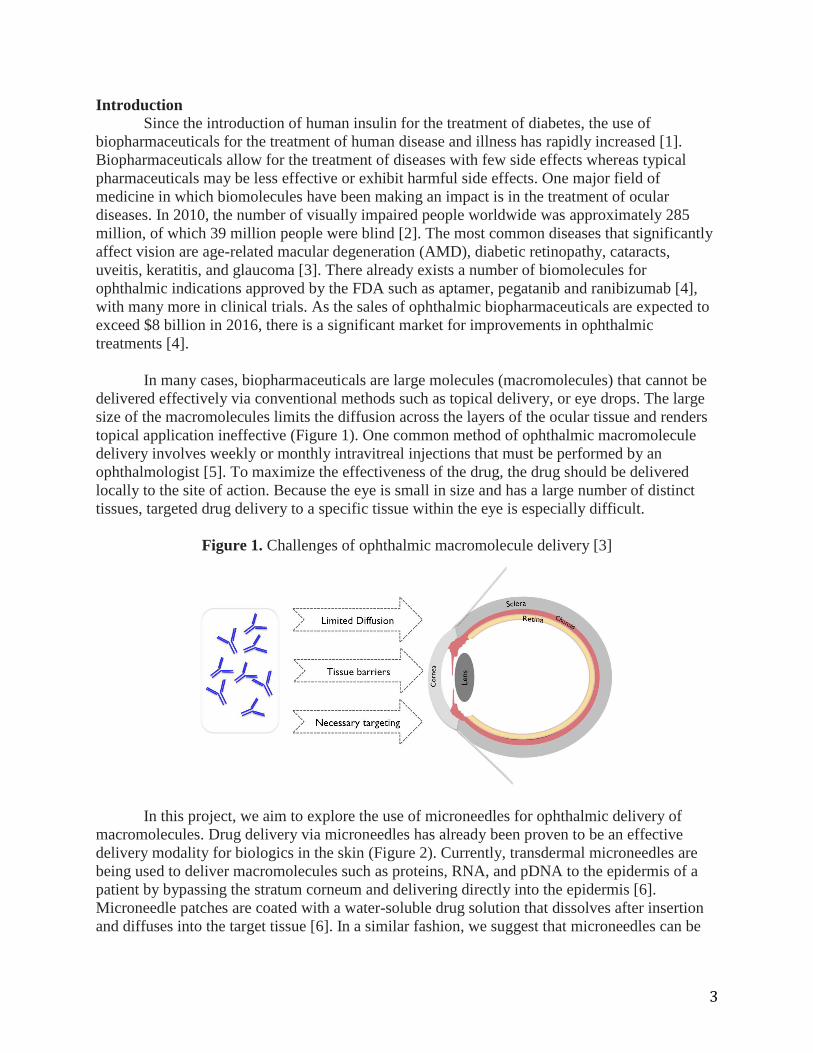
In many cases, biopharmaceuticals are large molecules (macromolecules) that cannot be

delivered effectively via conventional methods such as topical delivery, or eye drops. The large

size of the macromolecules limits the diffusion across the layers of the ocular tissue and renders

topical application ineffective (Figure 1). One common method of ophthalmic macromolecule

delivery involves weekly or monthly intravitreal injections that must be performed by an

ophthalmologist [5]. To maximize the effectiveness of the drug, the drug should be delivered

locally to the site of action. Because the eye is small in size and has a large number of distinct

tissues, targeted drug delivery to a specific tissue within the eye is especially difficult.

Figure 1. Challenges of ophthalmic macromolecule delivery [3]

In this project, we aim to explore the use of microneedles for ophthalmic delivery of

macromolecules. Drug delivery via microneedles has already been proven to be an effective

delivery modality for biologics in the skin (Figure 2). Currently, transdermal microneedles are

being used to deliver macromolecules such as proteins, RNA, and pDNA to the epidermis of a

patient by bypassing the stratum corneum and delivering directly into the epidermis [6].

Microneedle patches are coated with a water-soluble drug solution that dissolves after insertion

and diffuses into the target tissue [6]. In a similar fashion, we suggest that microneedles can be

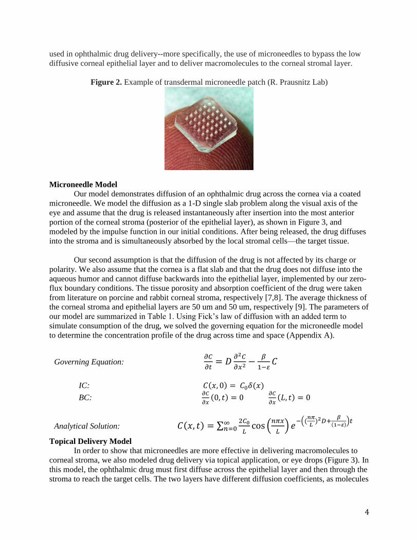
4

used in ophthalmic drug delivery--more specifically, the use of microneedles to bypass the low

diffusive corneal epithelial layer and to deliver macromolecules to the corneal stromal layer.

Figure 2. Example of transdermal microneedle patch (R. Prausnitz Lab)

Microneedle Model

Our model demonstrates diffusion of an ophthalmic drug across the cornea via a coated

microneedle. We model the diffusion as a 1-D single slab problem along the visual axis of the

eye and assume that the drug is released instantaneously after insertion into the most anterior

portion of the corneal stroma (posterior of the epithelial layer), as shown in Figure 3, and

modeled by the impulse function in our initial conditions. After being released, the drug diffuses

into the stroma and is simultaneously absorbed by the local stromal cells—the target tissue.

Our second assumption is that the diffusion of the drug is not affected by its charge or

polarity. We also assume that the cornea is a flat slab and that the drug does not diffuse into the

aqueous humor and cannot diffuse backwards into the epithelial layer, implemented by our zero-

flux boundary conditions. The tissue porosity and absorption coefficient of the drug were taken

from literature on porcine and rabbit corneal stroma, respectively [7,8]. The average thickness of

the corneal stroma and epithelial layers are 50 um and 50 um, respectively [9]. The parameters of

our model are summarized in Table 1. Using Fick’s law of diffusion with an added term to

simulate consumption of the drug, we solved the governing equation for the microneedle model

to determine the concentration profile of the drug across time and space (Appendix A).

Topical Delivery Model In order to show that microneedles are more effective in delivering macromolecules to

corneal stroma, we also modeled drug delivery via topical application, or eye drops (Figure 3). In

this model, the ophthalmic drug must first diffuse across the epithelial layer and then through the

stroma to reach the target cells. The two layers have different diffusion coefficients, as molecules

Governing Equation: 𝜕𝐶

𝜕𝑡= 𝐷

𝜕2𝐶

𝜕𝑥2−

𝛽

1−𝜀𝐶

IC: 𝐶(𝑥, 0) = 𝐶0𝛿(𝑥)

BC: 𝜕𝐶

𝜕𝑥(0, 𝑡) = 0

𝜕𝐶

𝜕𝑥(𝐿, 𝑡) = 0

Analytical Solution: 𝐶(𝑥, 𝑡) = ∑2𝐶0

𝐿cos (

𝑛𝜋𝑥

𝐿) 𝑒

−((𝑛𝜋

𝐿)2𝐷+

𝛽

(1−𝜀))𝑡∞

𝑛=0

5

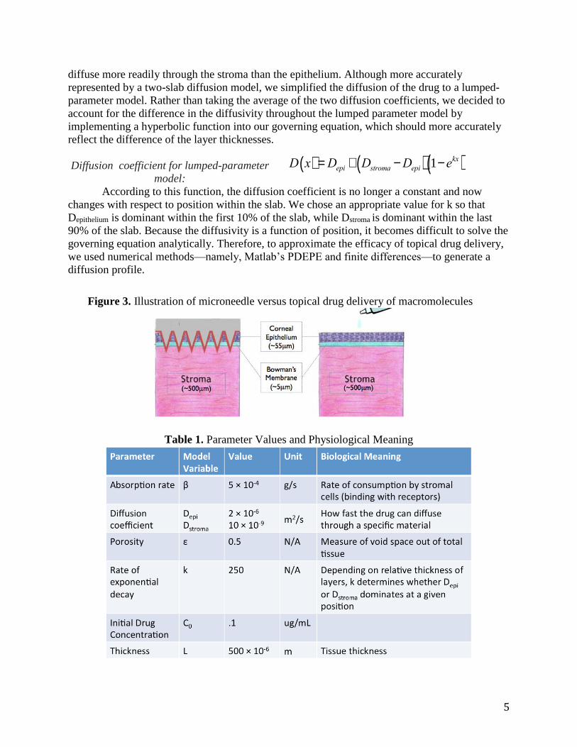
diffuse more readily through the stroma than the epithelium. Although more accurately

represented by a two-slab diffusion model, we simplified the diffusion of the drug to a lumped-

parameter model. Rather than taking the average of the two diffusion coefficients, we decided to

account for the difference in the diffusivity throughout the lumped parameter model by

implementing a hyperbolic function into our governing equation, which should more accurately

reflect the difference of the layer thicknesses.

Diffusion coefficient for lumped-parameter

model:

According to this function, the diffusion coefficient is no longer a constant and now

changes with respect to position within the slab. We chose an appropriate value for k so that

Depithelium is dominant within the first 10% of the slab, while Dstroma is dominant within the last

90% of the slab. Because the diffusivity is a function of position, it becomes difficult to solve the

governing equation analytically. Therefore, to approximate the efficacy of topical drug delivery,

we used numerical methods—namely, Matlab’s PDEPE and finite differences—to generate a

diffusion profile.

Table 1. Parameter Values and Physiological Meaning

D x( ) =Depi + Dstroma -Depi( ) 1-ekx( )

Figure 3. Illustration of microneedle versus topical drug delivery of macromolecules

6

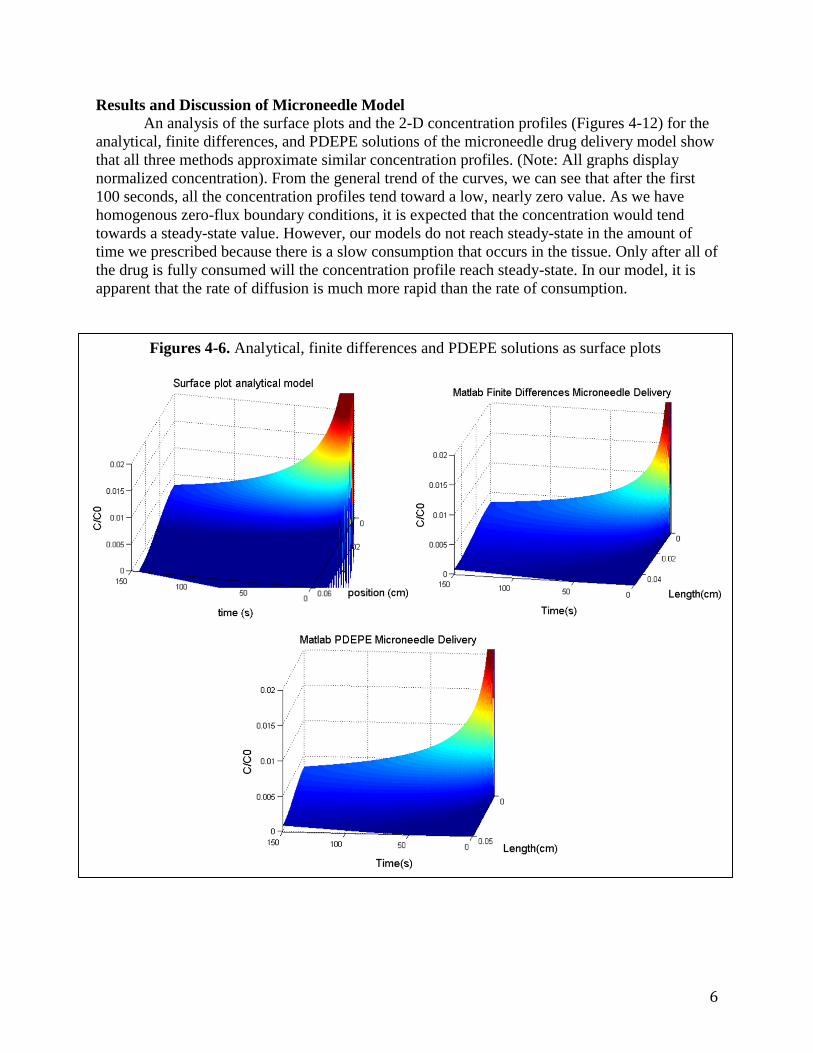
Results and Discussion of Microneedle Model

An analysis of the surface plots and the 2-D concentration profiles (Figures 4-12) for the

analytical, finite differences, and PDEPE solutions of the microneedle drug delivery model show

that all three methods approximate similar concentration profiles. (Note: All graphs display

normalized concentration). From the general trend of the curves, we can see that after the first

100 seconds, all the concentration profiles tend toward a low, nearly zero value. As we have

homogenous zero-flux boundary conditions, it is expected that the concentration would tend

towards a steady-state value. However, our models do not reach steady-state in the amount of

time we prescribed because there is a slow consumption that occurs in the tissue. Only after all of

the drug is fully consumed will the concentration profile reach steady-state. In our model, it is

apparent that the rate of diffusion is much more rapid than the rate of consumption.

Figures 4-6. Analytical, finite differences and PDEPE solutions as surface plots

7

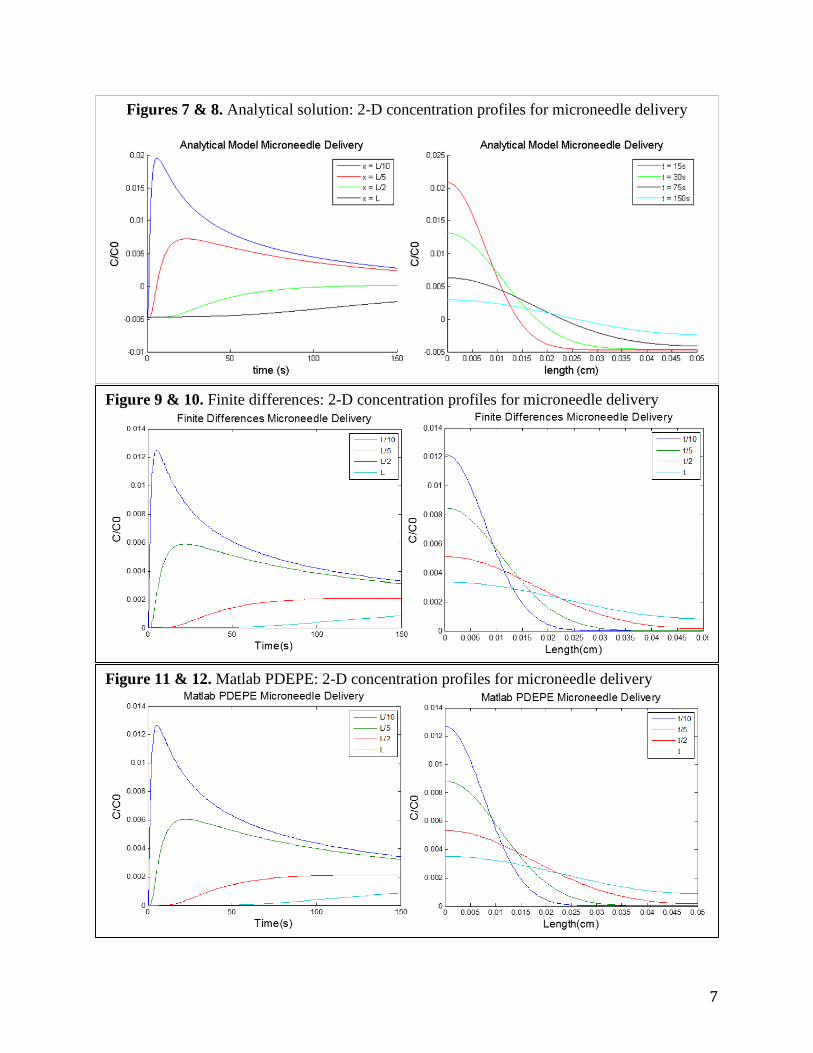
Figures 7 & 8. Analytical solution: 2-D concentration profiles for microneedle delivery

Figure 9 & 10. Finite differences: 2-D concentration profiles for microneedle delivery

Figure 11 & 12. Matlab PDEPE: 2-D concentration profiles for microneedle delivery

8

Both numerical methods approach about the same concentration values, peaking at

approximately 0.012 at both length L/10 and at time t/10 (Figures 9-12); the analytical method

demonstrates similar profiles, although the values were approximately 60% greater than those of

the numerical solutions, as shown by the peak value of 0.02 at length L/10 and time t/10 (15 s) in

Figures 7 and 8. This discrepancy may be due to the number of iterations run (n=100); a larger

number of iterations may help to more accurately reflect the solution. Although the two

numerical methods show very similar results, there are still slight differences in the values of

each method, which can be attributed to their respective limitations.

Limitations of Analytical, Finite Differences and PDEPE Methods

Using the analytical solution, Matlab cannot implement a dirac delta function and must

be approximated by an infinite summation; on the other hand, the numerical methods can

implement the dirac delta function relatively well. For the analytical model, we ran 100

iterations, which ignores all the higher eigenmodes. Theoretically, to achieve the most accurate

analytical solution, we would need to perform the summation over an infinite number of

iterations. Although the low number of iterations saves a great amount of computation time and

power, it comes at the detrimental cost of accuracy, which is evident in our model: the analytical

solution begins at a negative concentration due to the oscillatory behavior from the cosine term

and the position we chose to observe.

One major limitation of the finite differences method is that it is intolerant of changes to

dt and dx; reducing dx causes the step size to increase significantly, which requires a two-fold

decrease in dt to compensate. Thus, in order to achieve good spatial resolution, dx and dt must be

reduced, which causes an increase in number of time steps and computation time.

The greatest limitation of PDEPE is the number of iterations it can run before requiring

excessive computational time and power, similar to the limitations of the analytical and finite

differences method. Amongst the three methods, given a discrete amount of computational time

and power, PDEPE seemed to provide us with an accurate approximation of the solution with the

least amount of effort needed for optimization (unlike the required optimization of the number of

summations for the analytical solution, and of the step size for the finite differences method).

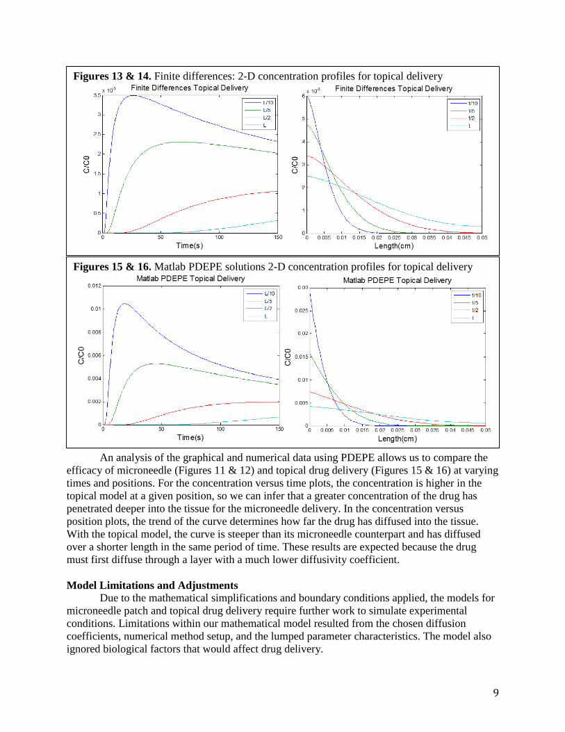
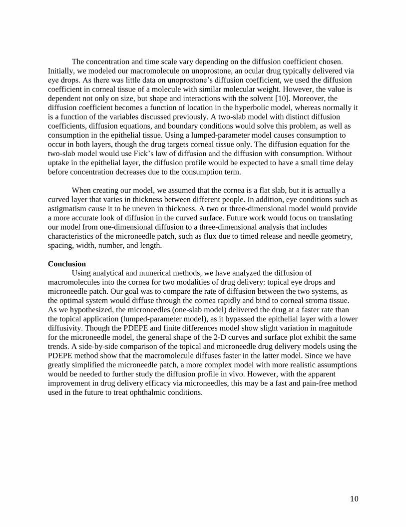
Results and Discussion of Topical Delivery Model

After verifying that the numerical methods provided good approximations of the

microneedle delivery profiles, we can now utilize these same methods to approximate the

solution to the governing equation of the topical delivery lumped-parameter model without

solving it analytically. Using the topical delivery model, limitations of the finite differences

methods become more apparent and significant. As seen previously, the finite differences

method is intolerant in of changes to parameter values. For example, if Dstroma is less than

Depithelium, the step size becomes a negative term, causing oscillations centered at zero. The finite

difference method is also limited by its nature: because the step size is a function of diffusivity,

and in turn the diffusivity of the lumped-parameter model is a function of position, the step size

changes with each iteration. With each iteration, errors accumulate, providing us with an

inaccurate approximation of the solution (Figures 13-16). Therefore, in order to compare the

microneedle delivery to the topical delivery, solely PDEPE was used.

9

An analysis of the graphical and numerical data using PDEPE allows us to compare the

efficacy of microneedle (Figures 11 & 12) and topical drug delivery (Figures 15 & 16) at varying

times and positions. For the concentration versus time plots, the concentration is higher in the

topical model at a given position, so we can infer that a greater concentration of the drug has

penetrated deeper into the tissue for the microneedle delivery. In the concentration versus

position plots, the trend of the curve determines how far the drug has diffused into the tissue.

With the topical model, the curve is steeper than its microneedle counterpart and has diffused

over a shorter length in the same period of time. These results are expected because the drug

must first diffuse through a layer with a much lower diffusivity coefficient.

Model Limitations and Adjustments

Due to the mathematical simplifications and boundary conditions applied, the models for

microneedle patch and topical drug delivery require further work to simulate experimental

conditions. Limitations within our mathematical model resulted from the chosen diffusion

coefficients, numerical method setup, and the lumped parameter characteristics. The model also

ignored biological factors that would affect drug delivery.

Figures 15 & 16. Matlab PDEPE solutions 2-D concentration profiles for topical delivery

Figures 13 & 14. Finite differences: 2-D concentration profiles for topical delivery

10

The concentration and time scale vary depending on the diffusion coefficient chosen.

Initially, we modeled our macromolecule on unoprostone, an ocular drug typically delivered via

eye drops. As there was little data on unoprostone’s diffusion coefficient, we used the diffusion

coefficient in corneal tissue of a molecule with similar molecular weight. However, the value is

dependent not only on size, but shape and interactions with the solvent [10]. Moreover, the

diffusion coefficient becomes a function of location in the hyperbolic model, whereas normally it

is a function of the variables discussed previously. A two-slab model with distinct diffusion

coefficients, diffusion equations, and boundary conditions would solve this problem, as well as

consumption in the epithelial tissue. Using a lumped-parameter model causes consumption to

occur in both layers, though the drug targets corneal tissue only. The diffusion equation for the

two-slab model would use Fick’s law of diffusion and the diffusion with consumption. Without

uptake in the epithelial layer, the diffusion profile would be expected to have a small time delay

before concentration decreases due to the consumption term.

When creating our model, we assumed that the cornea is a flat slab, but it is actually a

curved layer that varies in thickness between different people. In addition, eye conditions such as

astigmatism cause it to be uneven in thickness. A two or three-dimensional model would provide

a more accurate look of diffusion in the curved surface. Future work would focus on translating

our model from one-dimensional diffusion to a three-dimensional analysis that includes

characteristics of the microneedle patch, such as flux due to timed release and needle geometry,

spacing, width, number, and length.

Conclusion Using analytical and numerical methods, we have analyzed the diffusion of

macromolecules into the cornea for two modalities of drug delivery: topical eye drops and

microneedle patch. Our goal was to compare the rate of diffusion between the two systems, as

the optimal system would diffuse through the cornea rapidly and bind to corneal stroma tissue.

As we hypothesized, the microneedles (one-slab model) delivered the drug at a faster rate than

the topical application (lumped-parameter model), as it bypassed the epithelial layer with a lower

diffusivity. Though the PDEPE and finite differences model show slight variation in magnitude

for the microneedle model, the general shape of the 2-D curves and surface plot exhibit the same

trends. A side-by-side comparison of the topical and microneedle drug delivery models using the

PDEPE method show that the macromolecule diffuses faster in the latter model. Since we have

greatly simplified the microneedle patch, a more complex model with more realistic assumptions

would be needed to further study the diffusion profile in vivo. However, with the apparent

improvement in drug delivery efficacy via microneedles, this may be a fast and pain-free method

used in the future to treat ophthalmic conditions.

11

References

[1] Ryu, Jae Kuk, Hyo Sun Kim, and Doo Hyun Nam. "Current status and perspectives of

biopharmaceutical drugs." Biotechnology and Bioprocess Engineering 17.5 (2012): 900-911.

[2] Pascolini, Donatella, and Silvio Paolo Mariotti. "Global estimates of visual impairment:

2010." British Journal of Ophthalmology (2011): bjophthalmol-2011.

[3] Kim, Yoo Chun, et al. "Ocular delivery of macromolecules." Journal of Controlled

Release 190 (2014): 172-181.

[4] Syed, Basharut A., James B. Evans, and Leonard Bielory. "Wet AMD market."Nature

Reviews Drug Discovery 11.11 (2012): 827-827.

[5] El Sanharawi, M., et al. "Protein delivery for retinal diseases: from basic considerations to

clinical applications." Progress in retinal and eye research29.6 (2010): 443-465.

[6] Kim, Yeu-Chun, Jung-Hwan Park, and Mark R. Prausnitz. "Microneedles for drug and

vaccine delivery." Advanced drug delivery reviews 64.14 (2012): 1547-1568.

[7] Xiao, Jianhui, et al. "Construction of the recellularized corneal stroma using porous acellular

corneal scaffold." Biomaterials 32.29 (2011): 6962-6971.

[8] Kashiwagi, Kenji, Yoko Iizuka, and Shigeo Tsukahara. "Metabolites of isopropyl

unoprostone as potential ophthalmic solutions to reduce intraocular pressure in pigmented

rabbits." The Japanese Journal of Pharmacology 81.1 (1999): 56-62.

[9] Doughty, Michael J., and Mohammed L. Zaman. "Human corneal thickness and its impact on

intraocular pressure measures: a review and meta-analysis approach." Survey of

ophthalmology 44.5 (2000): 367-408.

[10] Zhang, Wensheng, Mark R. Prausnitz, and Aurélie Edwards. "Model of transient drug

diffusion across cornea." Journal of Controlled Release 99.2 (2004): 241-258.

12

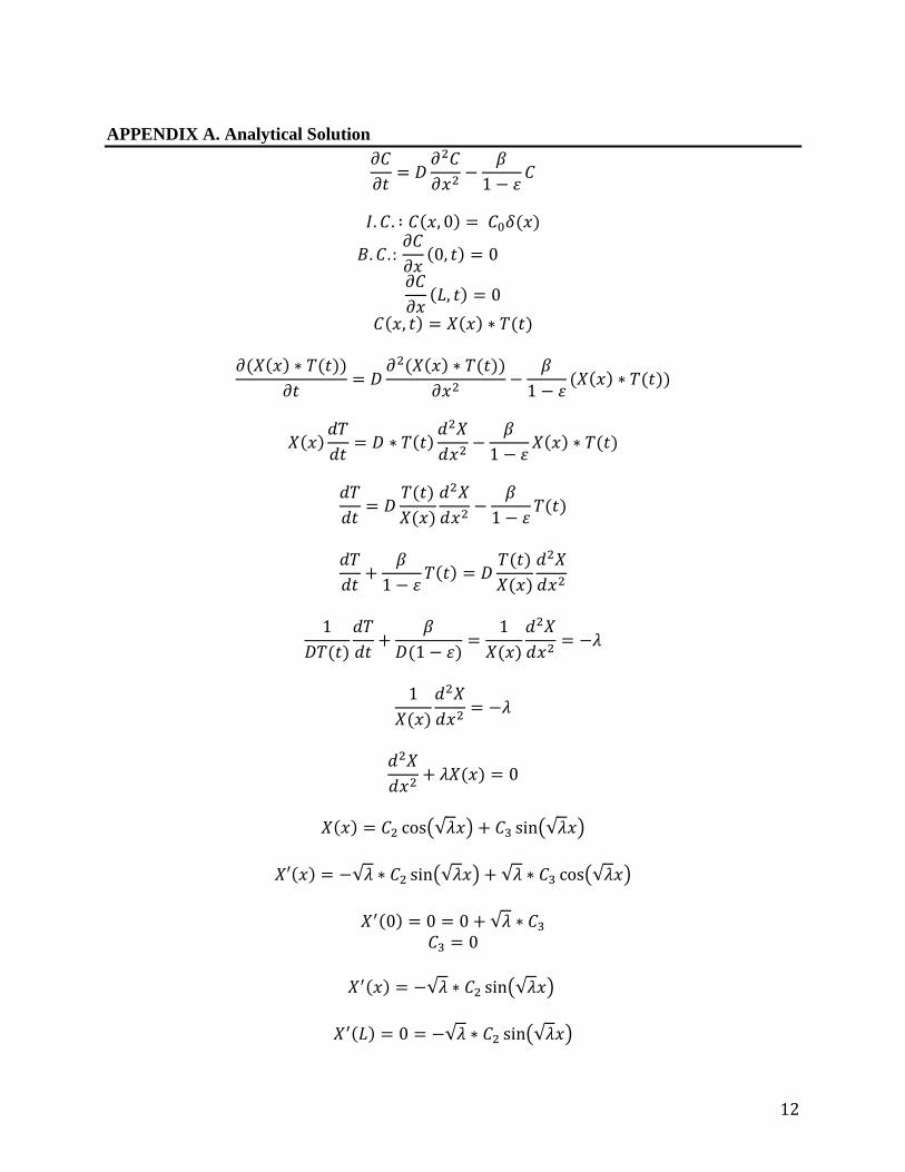
APPENDIX A. Analytical Solution

𝜕𝐶

𝜕𝑡= 𝐷

𝜕2𝐶

𝜕𝑥2−

𝛽

1 − 휀𝐶

𝐼. 𝐶. ∶ 𝐶(𝑥, 0) = 𝐶0𝛿(𝑥)

𝐵. 𝐶.: 𝜕𝐶

𝜕𝑥(0, 𝑡) = 0

𝜕𝐶

𝜕𝑥(𝐿, 𝑡) = 0

𝐶(𝑥, 𝑡) = 𝑋(𝑥) ∗ 𝑇(𝑡)

𝜕(𝑋(𝑥) ∗ 𝑇(𝑡))

𝜕𝑡= 𝐷

𝜕2(𝑋(𝑥) ∗ 𝑇(𝑡))

𝜕𝑥2−

𝛽

1 − 휀(𝑋(𝑥) ∗ 𝑇(𝑡))

𝑋(𝑥)𝑑𝑇

𝑑𝑡= 𝐷 ∗ 𝑇(𝑡)

𝑑2𝑋

𝑑𝑥2−

𝛽

1 − 휀𝑋(𝑥) ∗ 𝑇(𝑡)

𝑑𝑇

𝑑𝑡= 𝐷

𝑇(𝑡)

𝑋(𝑥)

𝑑2𝑋

𝑑𝑥2−

𝛽

1 − 휀𝑇(𝑡)

𝑑𝑇

𝑑𝑡+

𝛽

1 − 휀𝑇(𝑡) = 𝐷

𝑇(𝑡)

𝑋(𝑥)

𝑑2𝑋

𝑑𝑥2

1

𝐷𝑇(𝑡)

𝑑𝑇

𝑑𝑡+

𝛽

𝐷(1 − 휀)=

1

𝑋(𝑥)

𝑑2𝑋

𝑑𝑥2= −𝜆

1

𝑋(𝑥)

𝑑2𝑋

𝑑𝑥2= −𝜆

𝑑2𝑋

𝑑𝑥2+ 𝜆𝑋(𝑥) = 0

𝑋(𝑥) = 𝐶2 cos(√𝜆𝑥) + 𝐶3 sin(√𝜆𝑥)

𝑋′(𝑥) = −√𝜆 ∗ 𝐶2 sin(√𝜆𝑥) + √𝜆 ∗ 𝐶3 cos(√𝜆𝑥)

𝑋′(0) = 0 = 0 + √𝜆 ∗ 𝐶3 𝐶3 = 0

𝑋′(𝑥) = −√𝜆 ∗ 𝐶2 sin(√𝜆𝑥)

𝑋′(𝐿) = 0 = −√𝜆 ∗ 𝐶2 sin(√𝜆𝑥)

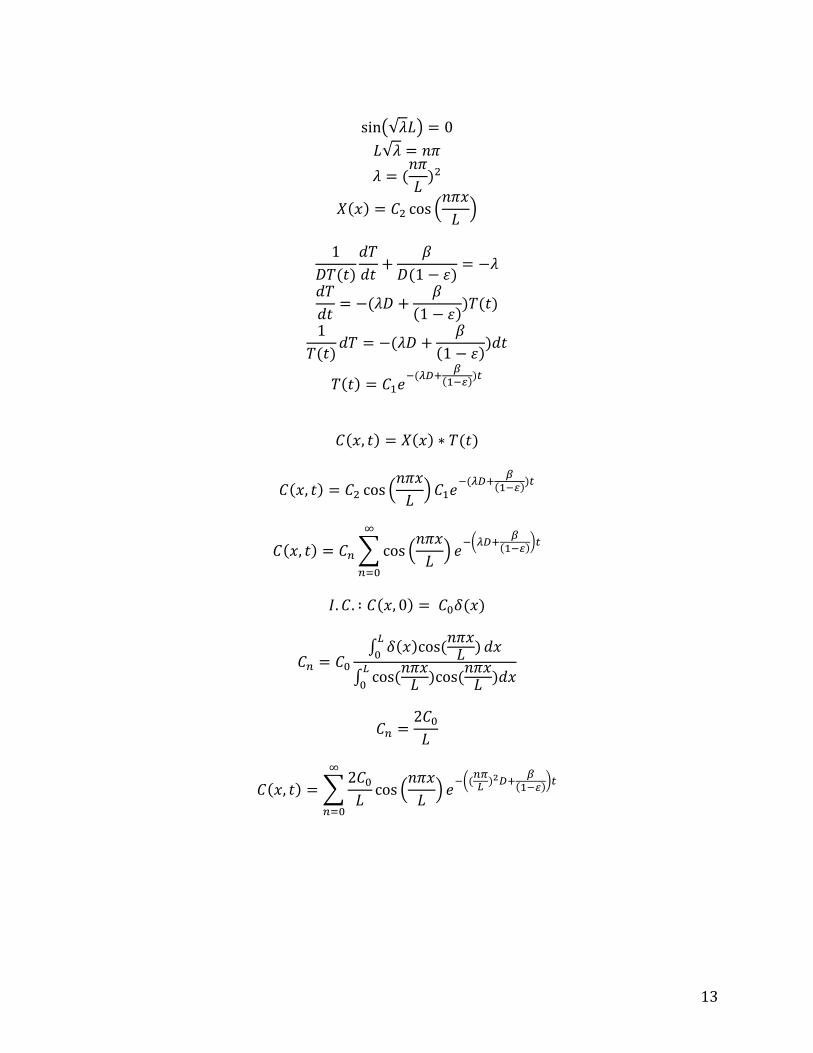
13

sin(√𝜆𝐿) = 0

𝐿√𝜆 = 𝑛𝜋

𝜆 = (𝑛𝜋

𝐿)2

𝑋(𝑥) = 𝐶2 cos (𝑛𝜋𝑥

𝐿)

1

𝐷𝑇(𝑡)

𝑑𝑇

𝑑𝑡+

𝛽

𝐷(1 − 휀)= −𝜆

𝑑𝑇

𝑑𝑡= −(𝜆𝐷 +

𝛽

(1 − 휀))𝑇(𝑡)

1

𝑇(𝑡)𝑑𝑇 = −(𝜆𝐷 +

𝛽

(1 − 휀))𝑑𝑡

𝑇(𝑡) = 𝐶1𝑒−(𝜆𝐷+

𝛽(1−𝜀)

)𝑡

𝐶(𝑥, 𝑡) = 𝑋(𝑥) ∗ 𝑇(𝑡)

𝐶(𝑥, 𝑡) = 𝐶2 cos (𝑛𝜋𝑥

𝐿) 𝐶1𝑒

−(𝜆𝐷+𝛽

(1−𝜀))𝑡

𝐶(𝑥, 𝑡) = 𝐶𝑛 ∑ cos (𝑛𝜋𝑥

𝐿) 𝑒

−(𝜆𝐷+𝛽

(1−𝜀))𝑡

∞

𝑛=0

𝐼. 𝐶. ∶ 𝐶(𝑥, 0) = 𝐶0𝛿(𝑥)

𝐶𝑛 = 𝐶0

∫ 𝛿(𝑥)cos (𝑛𝜋𝑥

𝐿 )𝐿

0𝑑𝑥

∫ cos (𝑛𝜋𝑥

𝐿 )cos (𝑛𝜋𝑥

𝐿 )𝑑𝑥𝐿

0

𝐶𝑛 =2𝐶0

𝐿

𝐶(𝑥, 𝑡) = ∑2𝐶0

𝐿cos (

𝑛𝜋𝑥

𝐿) 𝑒

−((𝑛𝜋𝐿

)2𝐷+𝛽

(1−𝜀))𝑡

∞

𝑛=0

14

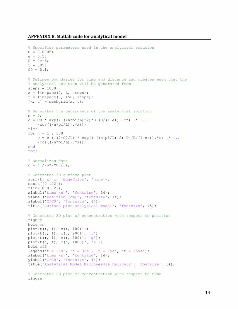
APPENDIX B. Matlab code for analytical model

% Specifies parameters used in the analytical solution B = 0.0005; e = 0.5; D = 2e-6; L = .05; C0 = 0.1;

% Defines boundaries for time and distance and creates mesh that the % analytical solution will be generated from steps = 1000; x = linspace(0, L, steps); t = linspace(0, 150, steps); [x, t] = meshgrid(x, t);

% Generates the datapoints of the analytical solution n = 0; c = C0 * exp((-((n*pi/L)^2)*D-(B/(1-e))).*t) .* ... (cos(((n*pi/L)).*x)); tic; for n = 1 : 100 c = c + (2*C0/L) * exp((-((n*pi/L)^2)*D-(B/(1-e))).*t) .* ... (cos(((n*pi/L)).*x)); end toc;

% Normalizes data c = c /(n*2*C0/L);

% Generates 3D surface plot surf(t, x, c, 'EdgeColor', 'none'); caxis([0 .02]); zlim([0 0.02]); xlabel('time (s)', 'fontsize', 14); ylabel('position (cm)', 'fontsize', 14); zlabel('C/C0', 'fontsize', 14); title('Surface plot analytical model', 'fontsize', 15);

% Generates 2D plot of concentration with respect to position figure hold on plot(t(:, 1), c(:, 100)'); plot(t(:, 1), c(:, 200)', 'r'); plot(t(:, 1), c(:, 500)', 'g'); plot(t(:, 1), c(:, 1000)', 'k'); hold off legend('t = 15s', 't = 30s', 't = 75s', 't = 150s'); xlabel('time (s)', 'fontsize', 14); ylabel('C/C0', 'fontsize', 14); title('Analytical Model Microneedle Delivery', 'fontsize', 14);

% Generates 2D plot of concentration with respect to time figure

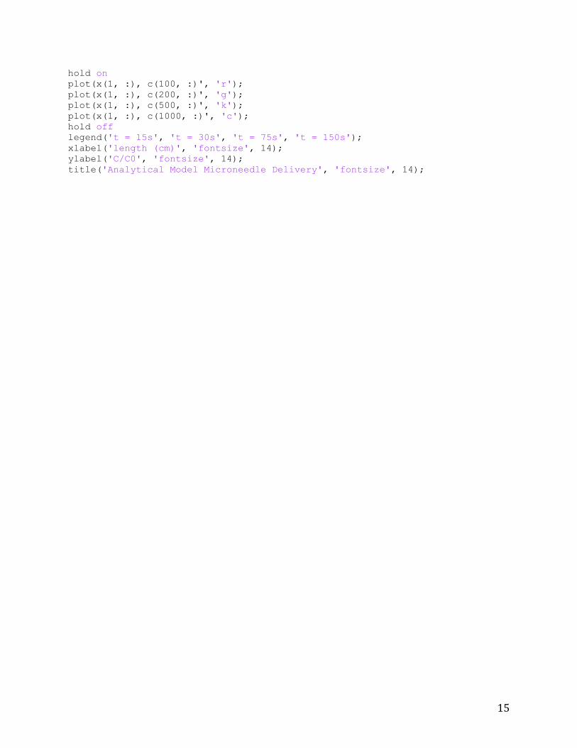
15

hold on plot(x(1, :), c(100, :)', 'r'); plot(x(1, :), c(200, :)', 'g'); plot(x(1, :), c(500, :)', 'k'); plot(x(1, :), c(1000, :)', 'c'); hold off legend('t = 15s', 't = 30s', 't = 75s', 't = 150s'); xlabel('length (cm)', 'fontsize', 14); ylabel('C/C0', 'fontsize', 14); title('Analytical Model Microneedle Delivery', 'fontsize', 14);

16

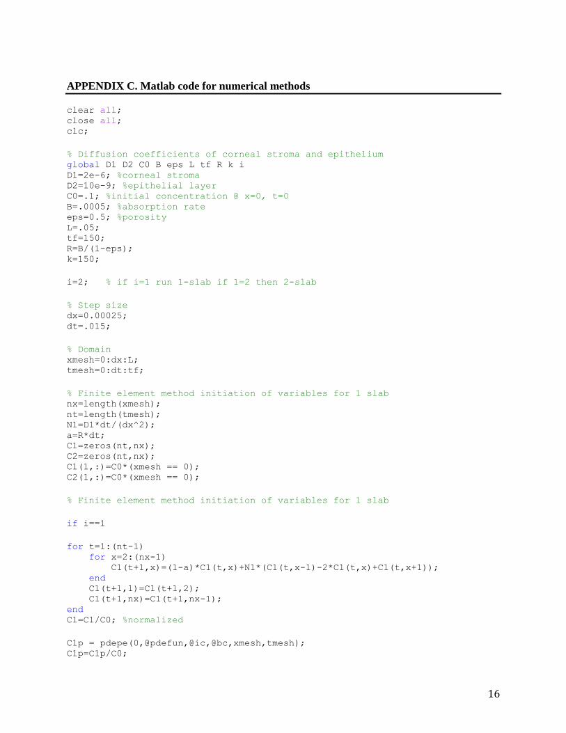
APPENDIX C. Matlab code for numerical methods

clear all;

close all; clc;

% Diffusion coefficients of corneal stroma and epithelium global D1 D2 C0 B eps L tf R k i D1=2e-6; %corneal stroma D2=10e-9; %epithelial layer C0=.1; %initial concentration @ x=0, t=0 B=.0005; %absorption rate eps=0.5; %porosity L=.05; tf=150; R=B/(1-eps); k=150;

i=2; % if i=1 run 1-slab if 1=2 then 2-slab

% Step size dx=0.00025; dt=.015;

% Domain xmesh=0:dx:L; tmesh=0:dt:tf;

% Finite element method initiation of variables for 1 slab nx=length(xmesh); nt=length(tmesh); N1=D1*dt/(dx^2); a=R*dt; C1=zeros(nt,nx); C2=zeros(nt,nx); C1(1,:)=C0*(xmesh == 0); C2(1,:)=C0*(xmesh == 0);

% Finite element method initiation of variables for 1 slab

if i==1

for t=1:(nt-1) for x=2:(nx-1) C1(t+1,x)=(1-a)*C1(t,x)+N1*(C1(t,x-1)-2*C1(t,x)+C1(t,x+1)); end C1(t+1,1)=C1(t+1,2); C1(t+1,nx)=C1(t+1,nx-1); end C1=C1/C0; %normalized

C1p = pdepe(0,@pdefun,@ic,@bc,xmesh,tmesh); C1p=C1p/C0;

17

figure (1) plot(tmesh,C1(:,floor(nx/10)),tmesh,C1(:,floor(nx/5)),tmesh,C1(:,floor(nx/2))

,tmesh,C1(:,floor(nx))); title('Finite Differences Microneedle Delivery','FontSize',14) xlabel('Time(s)','FontSize',14) ylabel('C/C0','FontSize',14) legend('L/10','L/5','L/2','L')

figure(2) plot(tmesh,C1p(:,floor(nx/10)),tmesh,C1p(:,floor(nx/5)),tmesh,C1p(:,floor(nx/

2)),tmesh,C1p(:,floor(nx))); title('Matlab PDEPE Microneedle Delivery','FontSize',14) xlabel('Time(s)','FontSize',14) ylabel('C/C0','FontSize',14) legend('L/10','L/5','L/2','L')

figure (3) plot(xmesh,C1(floor(nt/10),:),xmesh,C1(floor(nt/5),:),xmesh,C1(floor(nt/2),:)

,xmesh,C1(floor(nt),:)); title('Finite Differences Microneedle Delivery','FontSize',14) xlabel('Length(cm)','FontSize',14) ylabel('C/C0','FontSize',14) legend('t/10','t/5','t/2','t')

figure (4) plot(xmesh,C1p(floor(nt/10),:),xmesh,C1p(floor(nt/5),:),xmesh,C1p(floor(nt/2)

,:),xmesh,C1p(floor(nt),:)); title('Matlab PDEPE Microneedle Delivery','FontSize',14) xlabel('Length(cm)','FontSize',14) ylabel('C/C0','FontSize',14) legend('t/10','t/5','t/2','t')

figure(5)

H2=surf(tmesh,xmesh,C1p') title('Matlab PDEPE Microneedle Delivery','FontSize',14) xlabel('Time(s)','FontSize',14) ylabel('Length(cm)','FontSize',14) zlabel('C/C0','FontSize',14) set(H2, 'linestyle', 'none') axis([0 tf 0 L 0 .02 0 1]) caxis([0 .02])

else for t=1:(nt-1) for x=2:(nx-1) C2(t+1,x)=(1-a)*C2(t,x)+(dt/(dx^2))*(D2+(D1-D2)*(1-exp(-

k*x*dx)))*(C2(t,x+1)-2*C2(t,x)+C2(t,x-1));

end C2(t+1,1)=C2(t+1,2); C2(t+1,nx)=C2(t+1,nx-1); end

18

C2=C2/C0; %normalized C2p = pdepe(0,@pdefun,@ic,@bc,xmesh,tmesh); C2p=C2p/C0;

figure (1) plot(tmesh,C2(:,floor(nx/10)),tmesh,C2(:,floor(nx/5)),tmesh,C2(:,floor(nx/2))

,tmesh,C2(:,floor(nx))); title('Finite Differences Topical Delivery','FontSize',14) xlabel('Time(s)','FontSize',14) ylabel('C/C0','FontSize',14) legend('L/10','L/5','L/2','L')

figure(2) plot(tmesh,C2p(:,floor(nx/10)),tmesh,C2p(:,floor(nx/5)),tmesh,C2p(:,floor(nx/

2)),tmesh,C2p(:,floor(nx))); title('Matlab PDEPE Topical Delivery','FontSize',14) xlabel('Time(s)','FontSize',14) ylabel('C/C0','FontSize',14) legend('L/10','L/5','L/2','L')

figure (3) plot(xmesh,C2(floor(nt/10),:),xmesh,C2(floor(nt/5),:),xmesh,C2(floor(nt/2),:)

,xmesh,C2(floor(nt),:)); title('Finite Differences Topical Delivery','FontSize',14) xlabel('Length(cm)','FontSize',14) ylabel('C/C0','FontSize',14) legend('t/10','t/5','t/2','t')

figure (4) plot(xmesh,C2p(floor(nt/10),:),xmesh,C2p(floor(nt/5),:),xmesh,C2p(floor(nt/2)

,:),xmesh,C2p(floor(nt),:)); title('Matlab PDEPE Topical Delivery','FontSize',14) xlabel('Length(cm)','FontSize',14) ylabel('C/C0','FontSize',14) legend('t/10','t/5','t/2','t')

figure(5) H2=surf(tmesh,xmesh,C2p') title('Matlab PDEPE Topical Delivery','FontSize',14) xlabel('Time(s)','FontSize',14) ylabel('Length(cm)','FontSize',14) zlabel('C/C0','FontSize',14) set(H2, 'linestyle', 'none') axis([0 tf 0 L 0 .02 0 1]) caxis([0 .02])

end

function [c, f, s] = pdefun(x, t, u, DuDx)

global D1 R i D2 k

if i==1

c = 1;

19

f = D1 * DuDx; s = -R*u;

else

c = 1; f = (D2+(D1-D2)*(1-exp(-k*x)))*DuDx; s = -R*u;

end

end

function u0 = ic(x)

global C0 u0 = C0 * (x==0); %assumed instantaneous release

function [pl, ql, pr, qr] = bc(xl, ul, xr, ur, t)

pl = 0; %flux = 0 on needle side ql = 1; %flux = 0 on needle side pr = 0; %c = 0 on corneal end qr = 1; %flux = 0 on corneal end