MicroMAPS: From Storage to Flight
176
MicroMAPS: From Storage to Flight AOE 4066: Aircraft and Space Design Department of Aerospace and Ocean Engineering Virginia Polytechnic Institute and State University 5 May 2003 Team Members Adam Dubinskas Conor Haines Rivers Lamb Jennifer Lin Lee McCoy Shan Mohiuddin Christopher Nickell Monsid Poovantana Binh Tran Mike Tuttle Whitney Waldron Josh Zhou
Transcript of MicroMAPS: From Storage to Flight
MicroMAPS: From Storage to Flight
AOE 4066: Aircraft and Space Design
Department of Aerospace and Ocean Engineering
Virginia Polytechnic Institute and State University
5 May 2003
Team Members
Adam Dubinskas
Conor Haines
Rivers Lamb
Jennifer Lin
Lee McCoy
Shan Mohiuddin
Christopher Nickell
Monsid Poovantana
Binh Tran
Mike Tuttle
Whitney Waldron
Josh Zhou
ii
Table of Contents
List of Figures ............................................................................................................... vii
List of Tables................................................................................................................... x
List of Acronyms.......................................................................................................... xii
Chapter 1: Introduction and Problem Definition ................................................................ 1
1.1 MicroMAPS Information.......................................................................................... 1
1.1.1 MicroMAPS History.......................................................................................... 1
1.1.2 MicroMAPS Science Mission............................................................................ 2
1.1.3 MAPS History.................................................................................................... 2
1.1.4 MicroMAPS Physical Characteristics................................................................ 3
1.1.5 Descriptive Scenario .......................................................................................... 4
1.2 Problem Definition ................................................................................................... 4
1.2.1 Assessment of Scope.......................................................................................... 5
1.2.2 Required Disciplines .......................................................................................... 5
1.2.3 Societal Sectors and Actors Involved ................................................................ 6
1.2.4 Relevant and Subjective Elements..................................................................... 6
1.3 Needs, Alterables, and Constraints ........................................................................... 6
1.3.1 Proteus Mission Needs, Alterables, and Constraints ......................................... 7
1.3.2 Dedicated Aircraft Needs, Alterables, and Constraints ..................................... 8
1.3.3 Dedicated Spacecraft Needs, Alterables, and Constraints ................................. 9
1.4 Summary................................................................................................................. 10
Chapter 2: Value System Design ...................................................................................... 11
2.1 Proteus Objectives .................................................................................................. 11
2.1.1 Maximization of Performance ......................................................................... 11
2.1.2 Minimization of Cost ....................................................................................... 13
2.2 Dedicated Aircraft Objectives ................................................................................ 14
2.2.1 Maximization of Performance ......................................................................... 14
2.2.2 Minimization of Cost ....................................................................................... 16
2.3 Dedicated Spacecraft Objectives ............................................................................ 17
2.3.1 Maximization of Performance ......................................................................... 17
iii
2.3.2 Minimization of Cost ....................................................................................... 20
2.4 Summary................................................................................................................. 21
Chapter 3: Proteus.......................................................................................... 22
3.1 Mission Overview................................................................................................... 22
3.2 Power ...................................................................................................................... 23
3.2.1 System Overview ............................................................................................. 23
3.2.2 Main Power Converter NB50S41...................................................................... 26
3.2.3 PC104 Power Supply CB5S8 ........................................................................... 29
3.2.4 Triple Output MicroMAPS Power Supply NB45T41....................................... 30
3.2.5 EMI Filter NBF5041 ......................................................................................... 32
3.2.6 Heat Dissipation............................................................................................... 34
3.2.7 Wires, Connectors, and Line Diagram............................................................. 34
3.3 Data Acquisition ..................................................................................................... 37
3.3.1 Computer55 ....................................................................................................... 37
3.3.2 CPU Board ....................................................................................................... 37
3.3.3 Power Board..................................................................................................... 38
3.3.4 PC104 Enclosure.............................................................................................. 40
3.3.5 System Setup.................................................................................................... 41
3.4.1 1-Wire® Network14........................................................................................... 42
3.4.2 1-Wire® Serial Interface35 ................................................................................ 44
3.4.3 Thermal Compound ......................................................................................... 45
3.5 Structure.................................................................................................................. 45
3.5.1 Systems and Weights ....................................................................................... 46
3.5.2 MicroMAPS Viewing Window ....................................................................... 50
3.5.3 Instrument Suite Mounting Platform ............................................................... 51
3.5.4 Installation and Configuration ......................................................................... 53
4.1 Introduction............................................................................................................. 55
4.2 Aircraft RFP............................................................................................................ 55
4.3 Selection of Final Design Concept ......................................................................... 59
4.3.1 Menelaus I........................................................................................................ 59
4.3.2 Menelaus II ...................................................................................................... 60
iv
4.3.3 The Decision and Suggested Changes ............................................................. 61
4.4 Detailed Sizing........................................................................................................ 63
4.4.1 Sizing Process .................................................................................................. 64
4.4.2 Sizing Results................................................................................................... 69
4.5 Propulsion ............................................................................................................... 69
4.5.1 System Requirements....................................................................................... 69
4.5.2 Engine Selection .............................................................................................. 70
4.5.3 FJ44 Performance Characteristics.................................................................... 72
4.5.4 Engine Ducting ................................................................................................ 73
4.4.5 System Maintenance ........................................................................................ 74
4.6 Aerodynamics ......................................................................................................... 74
4.6.1 Configuration Design....................................................................................... 75
4.6.2 Airfoils ............................................................................................................. 77
4.6.3 Computational Aerodynamic Analysis ............................................................ 82
4.7 Stability and Control............................................................................................... 87
4.7.1 Justification of Configuration Geometry ......................................................... 87
4.7.2 Static Margin.................................................................................................... 89
4.7.3 Control Surface Sizing..................................................................................... 92
4.8 Performance ............................................................................................................ 95
4.8.1 Mission Profile Analysis.................................................................................. 95
4.8.2 Aircraft Comparison ........................................................................................ 97
4.9.1 Materials .......................................................................................................... 98
4.9.2 V-n Diagram .................................................................................................. 100
4.9.3 Wing Elements............................................................................................... 100
4.9.4 Fuselage ......................................................................................................... 101
4.9.5 Tail Booms..................................................................................................... 103
4.9.6 Weights Breakdown....................................................................................... 103
4.9.7 Center Of Gravity Travel ............................................................................... 104
4.10 Systems ............................................................................................................... 104
4.10.1 General Layout............................................................................................. 104
4.10.2 Payload System............................................................................................ 105
4.10.3 Fuel System.................................................................................................. 106

v
4.10.4 Landing Gear ............................................................................................... 106
4.10.5 Communication............................................................................................ 106
4.10.6 Avionics ....................................................................................................... 107
4.10.6 Flight Controls ............................................................................................. 107
4.11 Cost Analysis ...................................................................................................... 107
4.12 Final Proposal ..................................................................................................... 109
Chapter 5: Aiolos ............................................................................................................ 112
5.1 Orbit Design.......................................................................................................... 112
5.1.1 Specialized Orbits .......................................................................................... 112
5.1.2 Propulsion ...................................................................................................... 113
5.1.3 Altitude .......................................................................................................... 114
5.1.4 Inclination ...................................................................................................... 116
5.1.5 Orbit Determination System .......................................................................... 117
5.2 Attitude Determination and Control System (ADCS) .......................................... 118
5.2.1 Control Modes ............................................................................................... 119
5.2.2 Attitude Determination Components ............................................................. 119
5.2.3 Disturbance Torques ...................................................................................... 122
5.2.4 Attitude Control Components ........................................................................ 124
5.3 Power .................................................................................................................... 126
5.3.1 Operating Conditions and Requirements ....................................................... 127
5.3.2 Power Generation........................................................................................... 128
5.3.3 Energy Storage............................................................................................... 131
5.4 Command and Data Handling (C&DH) ............................................................... 132
5.5 Communication..................................................................................................... 133
5.5.1 Antenna .......................................................................................................... 133
5.5.2 Transmitter ..................................................................................................... 134
5.5.3 Receiver ......................................................................................................... 135
5.6 Thermal Management ........................................................................................... 136
5.6.1 Temperature Limits........................................................................................ 136
5.6.2 Heat Sources .................................................................................................. 137
5.6.3 Radiator.......................................................................................................... 138
5.6.4 Multi-Layered Insulation ............................................................................... 140
vi
5.7 Launch Vehicle ..................................................................................................... 141
5.7.1 Cost Comparison............................................................................................ 142
5.7.2 Athena II ........................................................................................................ 142
5.7.3 Delta II ........................................................................................................... 145
5.7.4 Taurus ............................................................................................................ 147
5.7.5 Comparison of Options .................................................................................. 150
5.8 Structures .............................................................................................................. 151
5.9 Cost Analysis ........................................................................................................ 157
5.10 Spacecraft Summary ........................................................................................... 157
References.................................................................................................................... 158
vii
List of Figures
Frontispiece: The Proteus Aircraft in Flight49
Figure 1: The MicroMAPS Instrument34 ............................................................................ 4
Figure 2: MicroMAPS power supply chassis10................................................................. 26
Figure 3: NB50S Main Converter Schematic41 ................................................................ 28
Figure 4: CB5S PC104 Power Supply Diagram8.............................................................. 30
Figure 5: NB45T MicroMAPS Power Supply41 ............................................................... 32
Figure 6: NBF50 EMI Filter Diagram41............................................................................ 33
Figure 7: Power System Connection Diagram.................................................................. 36
Figure 8: MZ104+ Mechanical Specifications55............................................................... 38
Figure 9: CT104 Enclosure – 6 inch depth55 .................................................................... 40
Figure 10: DS18S20 1-Wire® Digital Temperature Sensor14 ........................................... 43
Figure 11: HMP-2001S Digital Humidity Sensor (left) and............................................. 44
Figure 12: TEMP05 1-Wire® Serial Interface35................................................................ 45
Figure 13: PC104 Exterior Casing and Mounting Base (all dimensions in inches) ......... 47
Figure 14: MicroMAPS Diagram (inches) ....................................................................... 48
Figure 15: NBF50 Diagram (inches) ................................................................................ 48
Figure 16: CB5S Diagram (inches)................................................................................... 49
Figure 17: NB50S Diagram (inches) ................................................................................ 49
Figure 18: MicroMAPS Power Supply Diagram (inches)................................................ 49
Figure 19: External Pod Diagram ..................................................................................... 50
Figure 20: Base Platform Diagram, 6061-T6 Aluminum (inches) ................................... 51
Figure 21: Pod Mounting Configuration10........................................................................ 52
Figure 22: Endurance Mission Profile .............................................................................. 59
Figure 23: Menelaus I ....................................................................................................... 60
Figure 24: Menelaus II...................................................................................................... 61
Figure 25: New Configuration, Including Changes Developed in Decision Process ....... 64
Figure 26: Constraints Diagram to Optimize T/W and W/S............................................. 68
Figure 27: FJ44-1A Propulsion System62 ......................................................................... 71
Figure 28: FJ44-1A Variant Properties62 .......................................................................... 71
Figure 29: Net Thrust and SFC for FJ44 Variant ............................................................. 72
viii
Figure 30: Take-off Thrust under Varying Conditions..................................................... 73
Figure 31: The Main Wing Airfoil - NASA/Langley/Whitcomb LS(1)-0417 (GA(W))5778
Figure 32: The Tail Surface Airfoil - NACA 64-01257..................................................... 79
Figure 33: Main Wing Thickness-to-Chord Ratio and Wing Fuel Capacity .................... 80
Figure 34: Results from Boundary Layer Analysis .......................................................... 82
Figure 35: Model Layout and Pressure Distribution in Tornado...................................... 84
Figure 36: Numerical Data Generated by Tornado Iterations (all forces in Newtons)..... 85
Figure 37: Span Loading Generated by Tornado.............................................................. 86
Figure 38: Detail of the A-tail and Communications Pod ................................................ 88
Figure 39: Illustration of Roll-Yaw Coupling .................................................................. 89
Figure 40: Tornado-Generated Stability Derivatives........................................................ 91
Figure 41: Perseus B Aileron Size and Location39 ........................................................... 92
Figure 42: Menelaus Aileron Size and Location (all dimensions in ft)............................ 93
Figure 43: Predator B Ruddervator Size and Location39 .................................................. 94
Figure 44: Menelaus Ruddervator Size and Location (all dimensions in ft) .................... 94
Figure 45: Optimal Mission Profile .................................................................................. 96
Figure 46: V-n Diagram.................................................................................................. 100
Figure 47: Wing Structure .............................................................................................. 101
Figure 48: Fuselage Structure ......................................................................................... 102
Figure 49: Nose Cone Connection.................................................................................. 102
Figure 50: Center of Gravity Travel ............................................................................... 104
Figure 51: General Layout of Systems ........................................................................... 105
Figure 52: Landing Gear Arrangement (dimensions in ft) ............................................. 106
Figure 53: Percentage of RDT&E Cost .......................................................................... 108
Figure 54: Menelaus Three-View ................................................................................... 111
Figure 55: World Population Density63 .......................................................................... 116
Figure 56: SGR-20 Receiver and Antennas48 ................................................................. 118
Figure 57: Ithaco Conical Earth Sensor4......................................................................... 120
Figure 58: Surrey Two Axis Sun Sensor48...................................................................... 121
Figure 59: Ithaco IM-1034 .............................................................................................. 122
Figure 60: Ithaco Type A and B Wheels4 ....................................................................... 125
Figure 61: Ithaco Magnetic Torquers4 ............................................................................ 126
ix
Figure 62: S-band Quadrifilar Helix Antenna Footprint48.............................................. 134
Figure 63: Athena II Launch Vehicle3 ............................................................................ 143
Figure 64 Athena II Performance28................................................................................. 144
Figure 65: Athena II Payload Fairing28........................................................................... 144
Figure 66: Delta II Launch Vehicle Family15 ................................................................. 145
Figure 67: Delta II Launch Vehicle15.............................................................................. 146
Figure 68: Delta II 7920 Performance28.......................................................................... 146
Figure 69: Delta II Payload Fairings15 ............................................................................ 147
Figure 70: Taurus Launch Vehicle Family30 .................................................................. 148
Figure 71: Taurus Launch Vehicle30............................................................................... 148
Figure 72: Taurus Performance28.................................................................................... 149
Figure 73: Taurus Payload Fairing30............................................................................... 149
Figure 74: MicroMAPS Location within Aiolos ............................................................ 155
Figure 75: Complete Aiolos Configuration .................................................................... 156

x
List of Tables
Table 1: MicroMAPS Physical Characteristics59................................................................ 3
Table 2: General Needs, Alterables, and Constraints ......................................................... 7
Table 3: Proteus Mission Needs, Alterables, and Constraints ............................................ 8
Table 4: Dedicated Aircraft Needs, Alterables, and Constraints ........................................ 9
Table 5: Dedicated Spacecraft Needs, Alterables, and Constraints.................................... 9
Table 6: Proteus Performance Objectives......................................................................... 13
Table 7: Proteus Cost Objectives...................................................................................... 14
Table 8: Dedicated Aircraft Performance Objectives....................................................... 16
Table 9: Dedicated Aircraft Cost Objectives .................................................................... 17
Table 10: Dedicated Spacecraft Performance Objectives................................................. 20
Table 11: Dedicated Spacecraft Cost Objectives.............................................................. 21
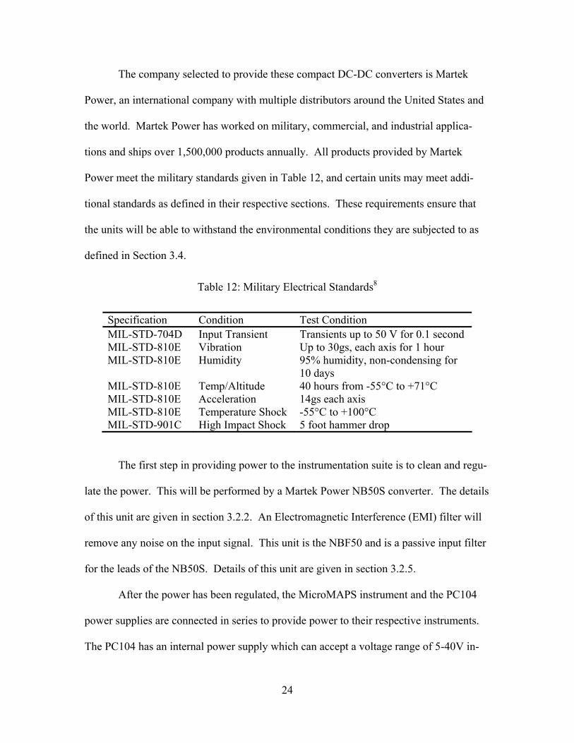
Table 12: Military Electrical Standards8........................................................................... 24
Table 13: NB50S Main Converter Details41 ..................................................................... 28
Table 14: CB5S PC104 Power Supply Details8................................................................ 29
Table 15: NB45T MicroMAPS Power Supply Details41................................................. 31
Table 16: NBF50 EMI Filter Details41.............................................................................. 33
Table 17: Heat generation................................................................................................. 34
Table 18: Electrical and Mechanical specifications of the HE10455 ................................ 39
Table 19: The Decision Matrix ......................................................................................... 62
Table 20: Estimation of CL ............................................................................................... 65
Table 21: Wing Loading and Span Loading ..................................................................... 65
Table 22: TOGW for Turbofan and Turboprop................................................................ 66
Table 23: TOGW Estimated from Existing Aircraft......................................................... 66
Table 24: Aspect Ratio Estimation ................................................................................... 67
Table 25: Thrust-to-Weight Ratio..................................................................................... 67
Table 26: Results of Aircraft Sizing Process .................................................................... 69
Table 27: Initial Engine Candidates62 ............................................................................... 70
Table 28: The Results from Friction Analysis for the Shortened Aircraft ....................... 77
Table 29: Input Data for Boundary Layer Analysis.......................................................... 81
Table 30: Final Aerodynamic Properties .......................................................................... 87
xi
Table 31: Menelaus Comparison ...................................................................................... 97
Table 32: Approximate Material Cost58............................................................................ 99
Table 33: Weight Summary ............................................................................................ 103
Table 34: Breakdown of RDT&E Cost Analysis............................................................ 108
Table 35: Comparison with RFP..................................................................................... 109
Table 36: Atmospheric Densities at Minimum Solar Activity 61.................................... 115
Table 37: Orbital Decay Calculations............................................................................. 115
Table 38: SGR-10 Data48 ................................................................................................ 118
Table 39: Ithaco Conical Earth Sensor Specifications4 .................................................. 120
Table 40: Surrey Sun Sensor Specifications48 ................................................................ 121
Table 41: Ithaco IM-103 Specifications4 ........................................................................ 122
Table 42: Disturbance Torque Equations Variable Definition ....................................... 123
Table 43: Disturbance Torque Calculations ................................................................... 124
Table 44: Attitude Actuator Calculations ....................................................................... 125
Table 45: Ithaco Wheel TW-16B32 Specifications4....................................................... 125
Table 46: Ithaco Magnetic Torquer TR30CFN Specifications4 ..................................... 126
Table 47: Subsystem Power Requirements..................................................................... 128
Table 48: Spectrolab Triple Junction Solar Cell Information56 ...................................... 129
Table 49: SAFT Lithium Ion Battery Information32....................................................... 131
Table 50: Operational Temperature Limit ...................................................................... 137
Table 51: Environmental Fluxes in Space23.................................................................... 138
Table 52: Internal Power Dissipation ............................................................................. 138
Table 53: Thermal Calculation Variables and Definitions ............................................. 140
Table 54: Launch Vehicle Cost Analysis61..................................................................... 142
Table 55: Launch Vehicle Selection Criteria3,15,28,30 ...................................................... 150
Table 56: Ranking of Launch Vehicles .......................................................................... 151
Table 57: Aluminum 7075-T73 Material Properties ...................................................... 152
Table 58: Launch Vehicle Structural Impact .................................................................. 153
Table 59: Launch Vehicle Dynamic Impact ................................................................... 154
Table 60: Subsystem Mass Summation .......................................................................... 155
Table 61: Inertia Calculations......................................................................................... 156
Table 62: Cost Analysis .................................................................................................. 157
xii
List of Acronyms
AC Alternating Current
ADCS Attitude Determination and Control System
BOL Beginning of Life
C&DH Command and Data Handling
CES Conical Earth Sensor
CG Center of Gravity
CO Carbon Monoxide
DARCO Defense Airborne Reconnaissance Office
DC Direct Current
DoD Department of Defense
DOD Depth of Discharge
EMI Electromagnetic Interference
EOL End of Life
ERAST Environmental Research Aircraft and Sensor Technology
FAA Federal Aviation Administration
GPS Global Positioning System
GTO Geosynchronous Transfer Orbit
HPA High Power Amplifier
IR Infrared
KLC Kodiak Launch Complex
KSC Kennedy Space Center
KTAS Knots True Airspeed
LaRC Langley Research Center
LELR Long Endurance Long Range
LEO Low Earth Orbit
MAPS Measurement of Air Pollution from Space
MLI Multi-Layer Insulation
NASA National Aeronautics and Space Administration
OH Hydroxyl Radical
OSR Optical Solar Reflectors
xiii
R&D Research and Development
RAM Random Access Memory
RFP Request for Proposal
ROM Read Only Memory
SGR Space GPS Receivers
SSLV Standard Small Launch Vehicle
SSTI Small Spacecraft Technology Initiative
SSTL Surrey Satellite Technology Ltd.
STS Space Shuttle Transportation System
TDRS Tracking and Data Relay Satellite
TFU Theoretical First Unit
TOGW Takeoff Gross Weight
UAV Unmanned Aerial Vehicle
VAFB Vandenberg Air Force Base
VSGC Virginia Space Grant Consortium
W/S Wing Loading
1
Chapter 1: Introduction and Problem Definition
The problem definition portion of the report provides background information for
the problem at hand. In addition, it sets the guidelines for the design process and the re-
quirements for the mission analyses that are completed. The establishment of these goals
leads to a more effective and efficient design process. This problem definition includes
basic information on the MicroMAPS instrument, a problem definition, and the needs,
alterables, and constraints of the mission.
1.1 MicroMAPS Information
Originally flown on the Space Shuttle in 1981, the MAPS (Measurement of Air
Pollution from Satellites) instrument measured carbon monoxide levels in the tropo-
sphere59. The MicroMAPS project was intended to be a longer duration, cheaper solution
meant to enhance the previous scientific results.59 Originally it was intended for use on
the Clark spacecraft, which was cancelled in 1998 as discussed below. Currently, re-
searchers at the National Aeronautics and Space Administration’s (NASA) Langley Re-
search Center (LaRC) are interested in flying the MicroMAPS instrument on the Proteus
research aircraft. The work of this design team includes designing the instrument inter-
face with the Proteus. In addition, dedicated aircraft and spacecraft are designed for the
MicroMAPS instrument, resulting in a final comparison between the three options.24
1.1.1 MicroMAPS History
In February 1998, NASA made the decision to terminate the Clark spacecraft be-
cause of mission costs, launch schedule delays, and concerns over on-orbit capabilities.40
As part of the Small Spacecraft Technology Initiative (SSTI), this mission was intended
2
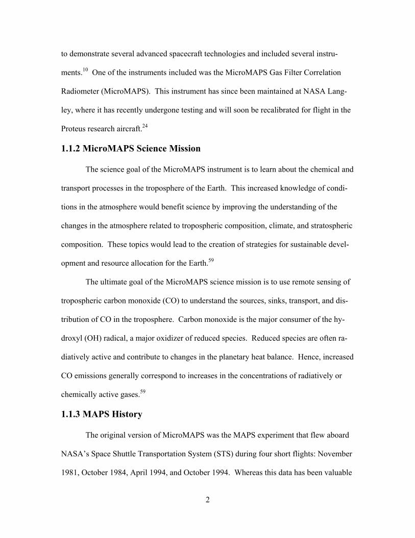
to demonstrate several advanced spacecraft technologies and included several instru-
ments.10 One of the instruments included was the MicroMAPS Gas Filter Correlation
Radiometer (MicroMAPS). This instrument has since been maintained at NASA Lang-
ley, where it has recently undergone testing and will soon be recalibrated for flight in the
Proteus research aircraft.24
1.1.2 MicroMAPS Science Mission
The science goal of the MicroMAPS instrument is to learn about the chemical and
transport processes in the troposphere of the Earth. This increased knowledge of condi-
tions in the atmosphere would benefit science by improving the understanding of the
changes in the atmosphere related to tropospheric composition, climate, and stratospheric
composition. These topics would lead to the creation of strategies for sustainable devel-
opment and resource allocation for the Earth.59
The ultimate goal of the MicroMAPS science mission is to use remote sensing of
tropospheric carbon monoxide (CO) to understand the sources, sinks, transport, and dis-
tribution of CO in the troposphere. Carbon monoxide is the major consumer of the hy-
droxyl (OH) radical, a major oxidizer of reduced species. Reduced species are often ra-
diatively active and contribute to changes in the planetary heat balance. Hence, increased
CO emissions generally correspond to increases in the concentrations of radiatively or
chemically active gases.59
1.1.3 MAPS History
The original version of MicroMAPS was the MAPS experiment that flew aboard
NASA’s Space Shuttle Transportation System (STS) during four short flights: November
1981, October 1984, April 1994, and October 1994. Whereas this data has been valuable
3
in establishing the variations of CO distributions, these missions had a maximum dura-
tion of 10 days and a latitude range of ± 57°. MicroMAPS was designed to be a smaller
and cheaper instrument that could collect global data with a lifetime goal of at least a
year. This information would improve the understanding of CO variations from season to
season and across variations in location.59
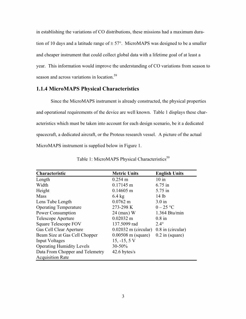
1.1.4 MicroMAPS Physical Characteristics
Since the MicroMAPS instrument is already constructed, the physical properties
and operational requirements of the device are well known. Table 1 displays these char-
acteristics which must be taken into account for each design scenario, be it a dedicated
spacecraft, a dedicated aircraft, or the Proteus research vessel. A picture of the actual
MicroMAPS instrument is supplied below in Figure 1.
Table 1: MicroMAPS Physical Characteristics59
Characteristic Metric Units English Units Length 0.254 m 10 in Width 0.17145 m 6.75 in Height 0.14605 m 5.75 in Mass 6.4 kg 14 lb Lens Tube Length 0.0762 m 3.0 in Operating Temperature 273-298 K 0 – 25 °C Power Consumption 24 (max) W 1.364 Btu/min Telescope Aperture 0.02032 m 0.8 in Square Telescope FOV 137.5099 rad 2.4° Gas Cell Clear Aperture 0.02032 m (circular) 0.8 in (circular) Beam Size at Gas Cell Chopper 0.00508 m (square) 0.2 in (square) Input Voltages 15, -15, 5 V Operating Humidity Levels 30-50% Data From Chopper and Telemetry Acquisition Rate
42.6 bytes/s

4
Figure 1: The MicroMAPS Instrument34
1.1.5 Descriptive Scenario
Successful implementation of the MicroMAPS instrument would be a tremendous
science asset. Whether onboard an aircraft or a spacecraft, this instrument would be able
to record vital information about carbon monoxide emissions and the transport processes
that are interrelated. This information is important in contributing to the understanding of
the Earth as a system. Scientists are likely to use this information both for confirming
other data as well as for the data itself.
1.2 Problem Definition
Due to the cancellation of the Clark spacecraft explained above, scientists at
LaRC have been searching for alternative platforms for MicroMAPS. While the decision
has been made to use the Proteus research aircraft, there is interest in comparing this op-
tion to the dedicated aircraft and spacecraft options. This section outlines the goals of
these three projects.

5
1.2.1 Assessment of Scope
The nature of the upcoming MicroMAPS mission requires that the first priority be
the successful integration of the instrument into the Proteus aircraft. This portion of the
project requires a thorough understanding of the characteristics of Proteus and the devel-
opment of an interface between the instrument and the aircraft. As such, the first task is
to design the structure and the subsystems required so that MicroMAPS can be operated
while flying onboard Proteus. A similar interface may be used for the design of the dedi-
cated aircraft and spacecraft. These two vehicles are designed specifically for the Mi-
croMAPS instrument and include all of the appropriate subsystems design and analysis.
These complete designs allow for a performance and cost comparison of the three op-
tions.
1.2.2 Required Disciplines
The scope as explained here involves many disciplines. Knowledge of atmos-
pheric sciences is required for an understanding of how MicroMAPS will behave in vary-
ing atmospheric conditions on the three possible platforms. Detailed electrical and com-
puter engineering work is necessary for development of the interface between Proteus
and MicroMAPS as well as the systems such as communications and command and data
handling on both the aircraft and spacecraft. In addition, a range of disciplines is re-
quired for the final designs: mission planning, trajectory analysis, aerodynamics, stability
and control, performance, structural design, power analysis, thermal management, and
project management. Aerospace engineering students in the aircraft and spacecraft de-
sign classes at Virginia Tech fill these roles.
6
1.2.3 Societal Sectors and Actors Involved
During this process, the engineering students at Virginia Tech have to interact
with other organizations and must consider the impact of design decisions. Contact with
NASA is vital to understand the science goals and restrictions of the MicroMAPS in-
strument. While other interactions with the agency are necessary, the primary contact is
LaRC, the center responsible for the instrumentation for atmospheric science data. Inter-
national laws must be upheld in all three MicroMAPS scenarios. Finally, public safety is
of paramount importance for the decisions made in planning these missions.
1.2.4 Relevant and Subjective Elements
As mentioned previously, the top priority for this project is to complete the design
of the structure that allows MicroMAPS to be integrated with the Proteus research air-
craft. This portion of the project is restrictive, as the existing MicroMAPS instrument
and the Proteus aircraft dictate the decisions that are made. Some of the subjective ele-
ments include the flight profile and the configuration of the Proteus and the method by
which MicroMAPS stores and transmits data.
The dedicated aircraft and spacecraft allow for a considerable amount of flexibil-
ity. The primary goal for these two missions is basic: to conduct a science mission using
the MicroMAPS instrument. Completion of this goal requires a thorough subsystem de-
sign and overall analysis of each mission. These decisions are left to the design team and
are reached after weighing the implications on the cost and performance for each case.
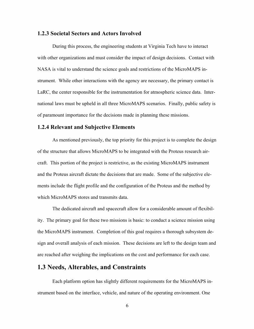
1.3 Needs, Alterables, and Constraints
Each platform option has slightly different requirements for the MicroMAPS in-
strument based on the interface, vehicle, and nature of the operating environment. One
7
way to analyze these requirements is through the tabulation of needs, alterables, and con-
straints. Compiling such a list provides a better understanding of what the goals are for
the project and what aspects can be changed. The needs category includes a simple defi-
nition of the problem; the alterables category includes those considerations that are
changed to meet the goals of the mission; and the constraints category includes the guide-
lines and restrictions that must be met by the mission. For the MicroMAPS project, there
are a few fundamental considerations and aspects which apply to all three scenarios. This
general list of needs, alterables, and constraints is included in Table 2.
Table 2: General Needs, Alterables, and Constraints
Category Element Needs: To develop and assess three distinct options for carrying out the sci-
ence mission for which the MicroMAPS instrument was built Alterables: Mission profile
Material selection Method of data acquisition
Method of data communication/storage Method of environmental protection
Constraints: Cost Vibration control Structural limits Attitude requirement: ± 2.5° of nadir pointing Attitude knowledge: ± 0.5° of nadir pointing Size and weight of instrument and supporting systems Project lifetime Atmospheric regulation: Relative humidity between 0% and 55% Temperature regulation: 32°F (0°C) and 77°F (25°C) Power requirements: 24 Watts, 5 V and ±15 V
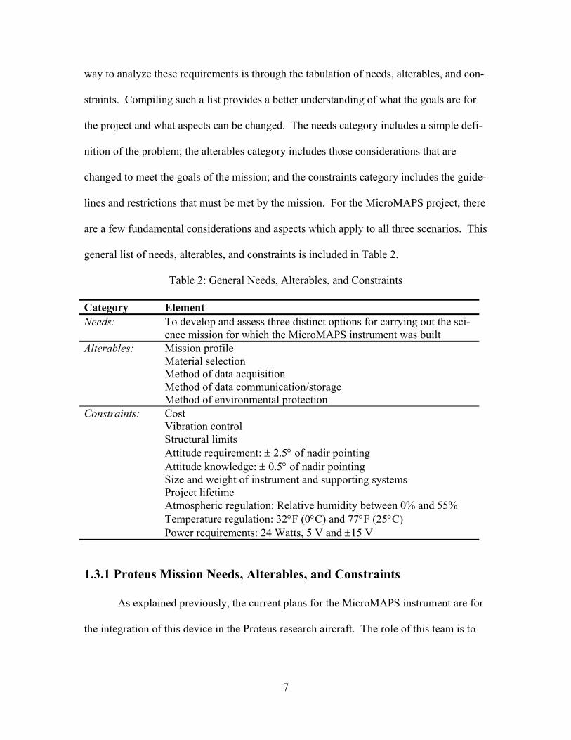
1.3.1 Proteus Mission Needs, Alterables, and Constraints
As explained previously, the current plans for the MicroMAPS instrument are for
the integration of this device in the Proteus research aircraft. The role of this team is to
8
design a system to provide an interface between the aircraft and the instrument. The
needs, alterables, and constraints that only apply to this portion of the project are listed in
Table 3.
Table 3: Proteus Mission Needs, Alterables, and Constraints
Category Element Needs: To provide an effective operating environment onboard the Proteus
aircraft for the MicroMAPS instrument Alterables: Location of instrument on airframe
Vehicle configuration Constraints: Prevention of contamination and condensation
Requirements of other missions on Proteus Proteus’s endurance/range: 14 hours at 500 NM radius (with 12500 lb takeoff weight) Rules and procedures for Proteus flights Power supplied by Proteus: 20 kW (continuous, thermal-managed)
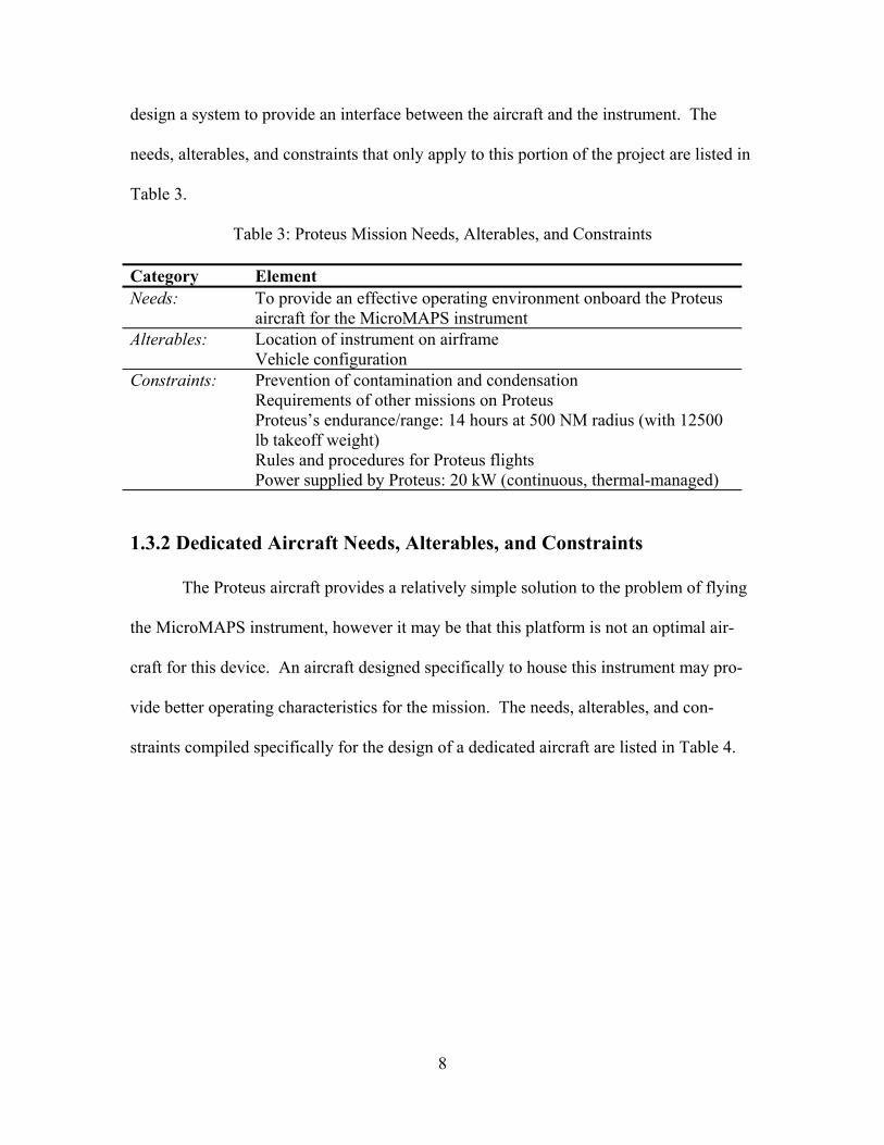
1.3.2 Dedicated Aircraft Needs, Alterables, and Constraints
The Proteus aircraft provides a relatively simple solution to the problem of flying
the MicroMAPS instrument, however it may be that this platform is not an optimal air-
craft for this device. An aircraft designed specifically to house this instrument may pro-
vide better operating characteristics for the mission. The needs, alterables, and con-
straints compiled specifically for the design of a dedicated aircraft are listed in Table 4.
9
Table 4: Dedicated Aircraft Needs, Alterables, and Constraints
Category Element Needs: To design a dedicated aircraft to carry out the science mission of the
MicroMAPS instrument Alterables: Aircraft type
Propulsion type Power source Geometric characteristics Support systems design
Constraints: Prevention of contamination and condensation Altitude requirement: 60,000 ft Endurance/range requirement: 40 hours at 1000 NM radius Lifespan of instrument in atmospheric flight conditions FAA compliant
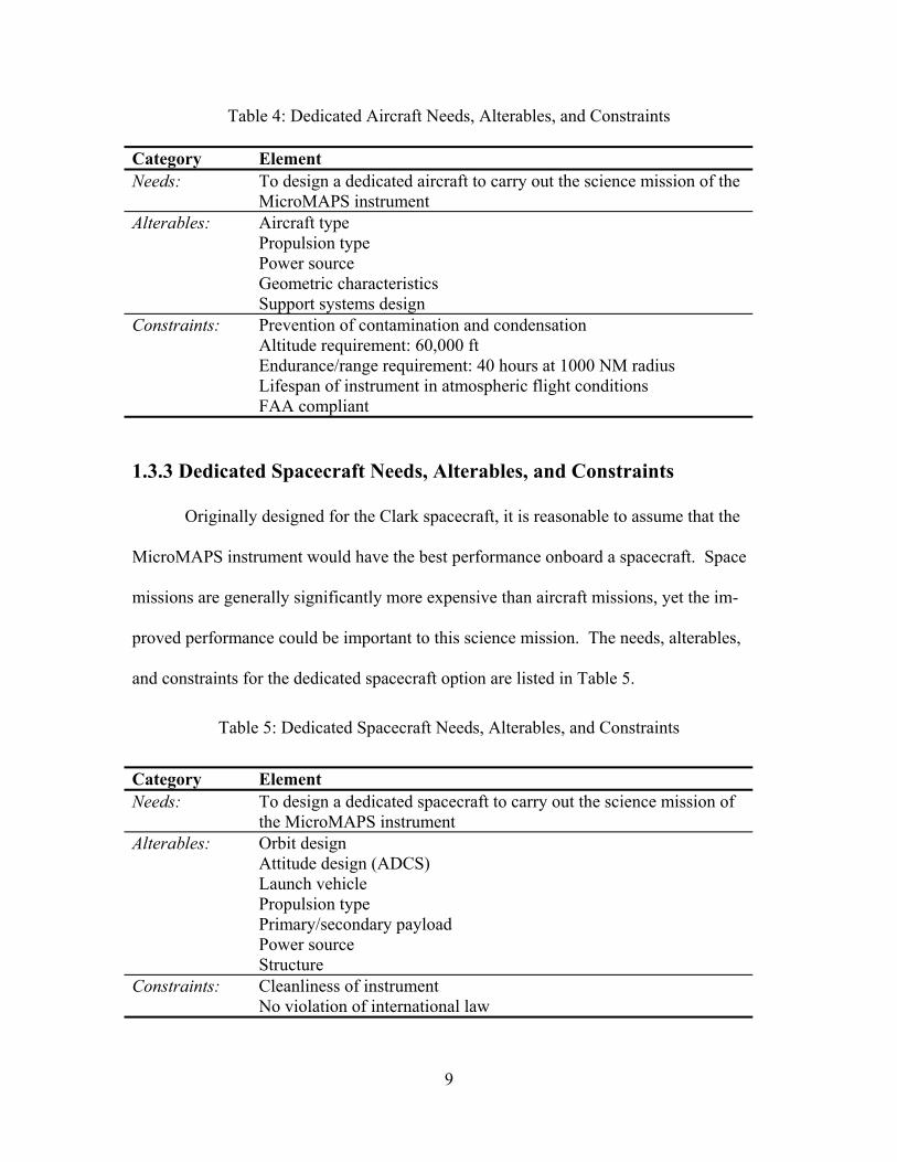
1.3.3 Dedicated Spacecraft Needs, Alterables, and Constraints
Originally designed for the Clark spacecraft, it is reasonable to assume that the
MicroMAPS instrument would have the best performance onboard a spacecraft. Space
missions are generally significantly more expensive than aircraft missions, yet the im-
proved performance could be important to this science mission. The needs, alterables,
and constraints for the dedicated spacecraft option are listed in Table 5.
Table 5: Dedicated Spacecraft Needs, Alterables, and Constraints
Category Element Needs: To design a dedicated spacecraft to carry out the science mission of
the MicroMAPS instrument Alterables: Orbit design
Attitude design (ADCS) Launch vehicle Propulsion type Primary/secondary payload Power source Structure
Constraints: Cleanliness of instrument No violation of international law

10
1.4 Summary
Chapter 1 gives an introduction to the history of the MicroMAPS instrument. It
explains the top priority of this design team, to design the interface that allows the sci-
ence mission to be conducted from the Proteus aircraft. In addition, the dedicated aircraft
and spacecraft options are presented, covering the options for comparison in this analysis.
Through the listing of needs, alterables, and constraints, the scope of each scenario is dis-
cussed. The following chapter discusses the value system design, leading to the detailed
analysis of each design option.
11
Chapter 2: Value System Design
One requirement of the design process is the development of guidelines which are
used to optimize the design. This value system design starts at the top level with two ba-
sic objectives: to maximize mission performance and to minimize mission cost. If these
two conditions are met, then the overall design is optimized. For each subsystem, there
are sub-objectives that fall into either the performance or cost categories. This section
presents these sub-objectives for each of the three possible platforms, and the manner in
which each objective can be measured.
2.1 Proteus Objectives
The Proteus design primarily involves the creation of the interface that supports
MicroMAPS in its mission on this research aircraft. As such, many constraints are al-
ready set. Yet, it is important to provide guidelines and a basis that is used in the analysis
and comparison of performance and cost for each possible option.
2.1.1 Maximization of Performance
Several subsystems must be optimized to maximize performance of the Proteus-
based operation of MicroMAPS. These include the thermal management system, the en-
vironmental control system, the power and electrical system, and the data acquisition and
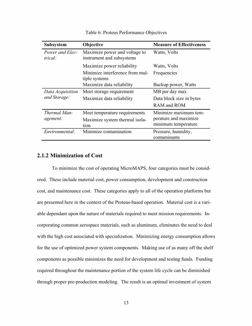
storage system. The performance requirements are compiled in Table 6.
The MicroMAPS interface guide stipulates that MicroMAPS be kept within a
specific internal temperature range of –5˚ C to 30˚ C to properly process incoming data.
Based on the expected mission profile of Proteus, the vehicle may encounter a tempera-
ture range of –57˚ C to 50˚ C during its total mission in the atmosphere. Designs that are
12
able to monitor and regulate the internal temperature range most efficiently will be val-
ued accordingly.
A proper operating environment is necessary for MicroMAPS to function cor-
rectly and minimize data corruption. In addition to the above temperature requirements,
other essential environmental properties of the MicroMAPS system include pressure and
humidity regulation. MicroMAPS requires a clean optical system in order to function
properly and minimize data corruption.
Another requirement is to supply power to all MicroMAPS instrument and inter-
face subsystems. The instrument requires a 24-Watt power supply capable of +5 and ±15
output voltages, and ideally, a backup power system could be included for redundancy.
A power management system is also required to control the power distribution and to en-
sure that the interference between other systems onboard the Proteus is kept to a mini-
mum.
Before any incoming signals are processed there must be a data storage system in
place to compile the information obtained during flight, complemented by a backup stor-
age system. The instrument is able to gather a maximum of 0.432 MB of data per day,
which will be extracted following each mission.
13
Table 6: Proteus Performance Objectives
Subsystem Objective Measure of Effectiveness Maximize power and voltage to instrument and subsystems
Watts, Volts
Maximize power reliability Watts, Volts Minimize interference from mul-tiple systems
Frequencies
Power and Elec-trical:
Maximize data reliability Backup power, Watts Meet storage requirement MB per day max Maximize data reliability Data block size in bytes
Data Acquisition and Storage:
RAM and ROM Meet temperature requirements Thermal Man-
agement: Maximize system thermal isola-tion
Minimize maximum tem-perature and maximize minimum temperature
Environmental: Minimize contamination Pressure, humidity, contaminants
2.1.2 Minimization of Cost
To minimize the cost of operating MicroMAPS, four categories must be consid-
ered. These include material cost, power consumption, development and construction
cost, and maintenance cost. These categories apply to all of the operation platforms but
are presented here in the context of the Proteus-based operation. Material cost is a vari-
able dependant upon the nature of materials required to meet mission requirements. In-
corporating common aerospace materials, such as aluminum, eliminates the need to deal
with the high cost associated with specialization. Minimizing energy consumption allows
for the use of optimized power system components. Making use of as many off the shelf
components as possible minimizes the need for development and testing funds. Funding
required throughout the maintenance portion of the system life cycle can be diminished
through proper pre-production modeling. The result is an optimal investment of system
14
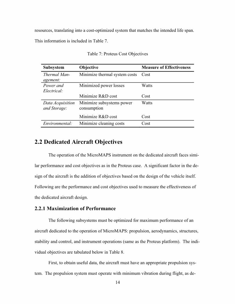
resources, translating into a cost-optimized system that matches the intended life span.
This information is included in Table 7.
Table 7: Proteus Cost Objectives
Subsystem Objective Measure of Effectiveness Thermal Man-agement:
Minimize thermal system costs Cost
Power and Electrical:
Minimized power losses Watts
Minimize R&D cost Cost Data Acquisition and Storage:
Minimize subsystems power consumption
Watts
Minimize R&D cost Cost Environmental: Minimize cleaning costs Cost
2.2 Dedicated Aircraft Objectives
The operation of the MicroMAPS instrument on the dedicated aircraft faces simi-
lar performance and cost objectives as in the Proteus case. A significant factor in the de-
sign of the aircraft is the addition of objectives based on the design of the vehicle itself.
Following are the performance and cost objectives used to measure the effectiveness of
the dedicated aircraft design.
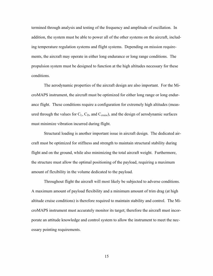
2.2.1 Maximization of Performance
The following subsystems must be optimized for maximum performance of an
aircraft dedicated to the operation of MicroMAPS: propulsion, aerodynamics, structures,
stability and control, and instrument operations (same as the Proteus platform). The indi-
vidual objectives are tabulated below in Table 8.
First, to obtain useful data, the aircraft must have an appropriate propulsion sys-
tem. The propulsion system must operate with minimum vibration during flight, as de-
15
termined through analysis and testing of the frequency and amplitude of oscillation. In
addition, the system must be able to power all of the other systems on the aircraft, includ-
ing temperature regulation systems and flight systems. Depending on mission require-
ments, the aircraft may operate in either long endurance or long range conditions. The
propulsion system must be designed to function at the high altitudes necessary for these
conditions.
The aerodynamic properties of the aircraft design are also important. For the Mi-
croMAPS instrument, the aircraft must be optimized for either long range or long endur-
ance flight. These conditions require a configuration for extremely high altitudes (meas-
ured through the values for CL, CD, and Ccruise), and the design of aerodynamic surfaces
must minimize vibration incurred during flight.
Structural loading is another important issue in aircraft design. The dedicated air-
craft must be optimized for stiffness and strength to maintain structural stability during
flight and on the ground, while also minimizing the total aircraft weight. Furthermore,
the structure must allow the optimal positioning of the payload, requiring a maximum
amount of flexibility in the volume dedicated to the payload.
Throughout flight the aircraft will most likely be subjected to adverse conditions.
A maximum amount of payload flexibility and a minimum amount of trim drag (at high
altitude cruise conditions) is therefore required to maintain stability and control. The Mi-
croMAPS instrument must accurately monitor its target; therefore the aircraft must incor-
porate an attitude knowledge and control system to allow the instrument to meet the nec-
essary pointing requirements.
16
In addition to these requirements, the dedicated aircraft must meet certain tem-
perature, power, and data storage requirements as dictated by the MicroMAPS instru-
ment. These constraints are described in detail in Section 1.3.
Table 8: Dedicated Aircraft Performance Objectives
Subsystem Objective Measure of Effectiveness Aerodynamics: Optimize for long
range/endurance (L/D)max (E)
(D/V) (R) Optimize for high altitude CL, CD, Vcruise Minimize vibration Frequency and amplitude Stability and Maximize payload flexibility Static margin Control: Minimize trim drag (high alti-
tude) CM at high altitude
Structures: Optimize strength Material/configuration yield strength
Minimize weight (high alti-tude)
Material density and volume
Maximize payload flexibility Available payload volume Optimize stiffness Material/configuration Young's
Modulus Propulsion: Minimize vibration Frequency and amplitude Maximize power for instru-
ment & subsystems Watts
Optimize for high altitude (L/D)max, Wmin T=(D/L)*W Optimize for long
range/endurance Distance/vol. of fuel or time/vol. of fuel
2.2.2 Minimization of Cost
There are certain issues to consider when trying to minimize the cost of the dedi-
cated aircraft. Certainly all of the ways to minimize the cost associated with the instru-
ment operation as mentioned in the Proteus section of this chapter are applicable here as
well. Specific aircraft design choices rely on adherence to the NASA mission goals and
most notably require a long range and high endurance aircraft. Aircraft parameters that
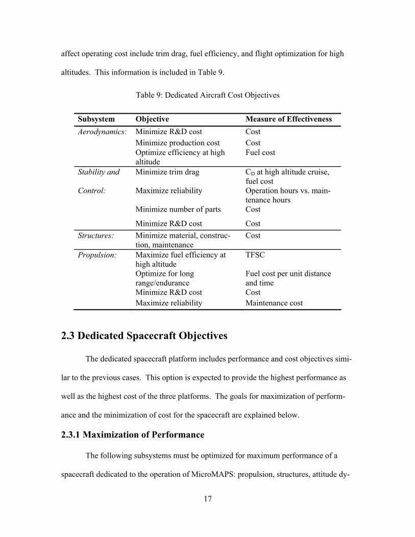
17
affect operating cost include trim drag, fuel efficiency, and flight optimization for high
altitudes. This information is included in Table 9.
Table 9: Dedicated Aircraft Cost Objectives
Subsystem Objective Measure of Effectiveness Aerodynamics: Minimize R&D cost Cost Minimize production cost Cost Optimize efficiency at high
altitude Fuel cost
Stability and Minimize trim drag CD at high altitude cruise, fuel cost
Control: Maximize reliability Operation hours vs. main-tenance hours
Minimize number of parts Cost
Minimize R&D cost Cost Structures: Minimize material, construc-
tion, maintenance Cost
Propulsion: Maximize fuel efficiency at high altitude
TFSC
Optimize for long range/endurance
Fuel cost per unit distance and time
Minimize R&D cost Cost Maximize reliability Maintenance cost
2.3 Dedicated Spacecraft Objectives
The dedicated spacecraft platform includes performance and cost objectives simi-
lar to the previous cases. This option is expected to provide the highest performance as
well as the highest cost of the three platforms. The goals for maximization of perform-
ance and the minimization of cost for the spacecraft are explained below.
2.3.1 Maximization of Performance
The following subsystems must be optimized for maximum performance of a
spacecraft dedicated to the operation of MicroMAPS: propulsion, structures, attitude dy-
18
namics and control, launch vehicle, and instrument operations (same as the Proteus plat-
form). The performance objectives of the dedicated spacecraft are compiled in Table 10.
One of the primary advantages of the dedicated spacecraft in the application of
MicroMAPS is the ability to monitor a relatively large area for a long period of time.
Depending on the scientific goals, it may be necessary to include a propulsion system ca-
pable of efficiently changing or modifying the orbit of the spacecraft.
The MicroMAPS instrument operates at an ideal state under “clean” conditions.
A space mission is not exposed to the same atmospheric conditions as Proteus or the
dedicated spacecraft. Therefore the environment under which MicroMAPS is to be inte-
grated into the spacecraft must be clean to minimize contaminants within the instrument
itself. Such contaminants compromise the quality of the data obtained during missions.
The spacecraft will be exposed to temperature ranges exceeding those for which
MicroMAPS is designed. Therefore, a thermal management system must be in place to
measure and regulate the temperature of the instrument. The system must also monitor
the heat produced by auxiliary systems and thermal radiation from the operating envi-
ronment.
The MicroMAPS instrument must be pointed correctly to obtain useful data. The
instrument requires that the spacecraft have an attitude determination and control system
capable of ensuring that the attitude control of MicroMAPS is within ±2.5˚ and that the
attitude knowledge error is no greater than ±0.5˚.
During launch and operation, the MicroMAPS instrument and the spacecraft will
be subjected to varying loads. The structural design must be sufficient to withstand the
anticipated loading from the launch vehicle. The stiffness of the structure must be such
19
that the vibration of the spacecraft is minimized. A maximum amount of payload flexi-
bility would allow different configurations to be used for a variety of situations.
A launch vehicle is required to place the spacecraft in low earth orbit (LEO). The
launch vehicle must be selected to minimize the forces acting on the spacecraft during
launch. Lower launch loads correlate to a lower total spacecraft mass.
The same temperature and power requirements of the instrument that were men-
tioned previously in the Proteus section of this chapter, also apply to the spacecraft. The
instrument gathers a maximum of 0.432 MB of data, and the spacecraft must have the
capability to transmit the data periodically to a ground station. The power used by the
transmission and storage system must be kept to a minimum.
20
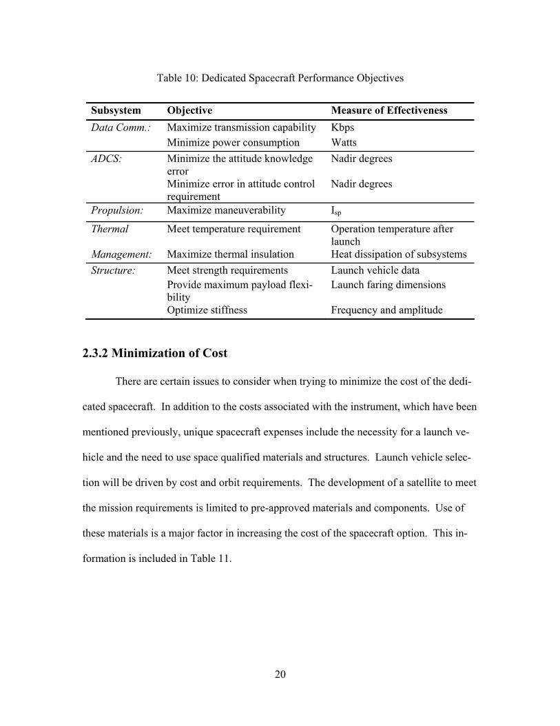
Table 10: Dedicated Spacecraft Performance Objectives
Subsystem Objective Measure of Effectiveness Data Comm.: Maximize transmission capability Kbps Minimize power consumption Watts ADCS: Minimize the attitude knowledge
error Nadir degrees
Minimize error in attitude control requirement
Nadir degrees
Propulsion: Maximize maneuverability Isp
Thermal Meet temperature requirement Operation temperature after launch
Management: Maximize thermal insulation Heat dissipation of subsystems Structure: Meet strength requirements Launch vehicle data Provide maximum payload flexi-
bility Launch faring dimensions
Optimize stiffness Frequency and amplitude
2.3.2 Minimization of Cost
There are certain issues to consider when trying to minimize the cost of the dedi-
cated spacecraft. In addition to the costs associated with the instrument, which have been
mentioned previously, unique spacecraft expenses include the necessity for a launch ve-
hicle and the need to use space qualified materials and structures. Launch vehicle selec-
tion will be driven by cost and orbit requirements. The development of a satellite to meet
the mission requirements is limited to pre-approved materials and components. Use of
these materials is a major factor in increasing the cost of the spacecraft option. This in-
formation is included in Table 11.
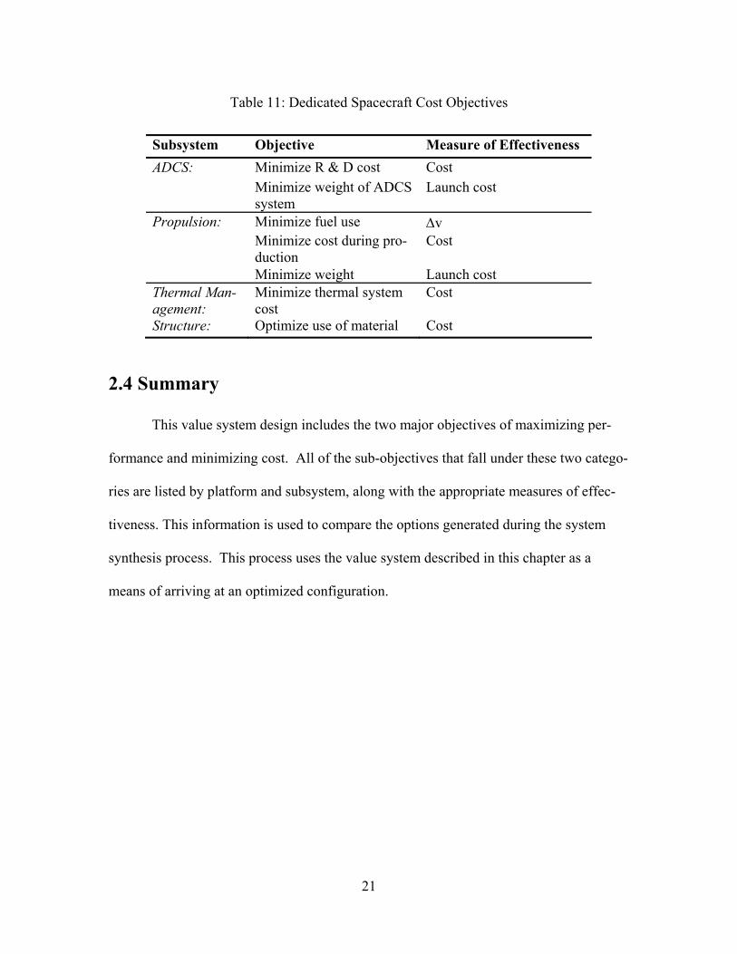
21
Table 11: Dedicated Spacecraft Cost Objectives
Subsystem Objective Measure of Effectiveness ADCS: Minimize R & D cost Cost Minimize weight of ADCS
system Launch cost
Propulsion: Minimize fuel use ∆v Minimize cost during pro-
duction Cost
Minimize weight Launch cost Thermal Man-agement:
Minimize thermal system cost
Cost
Structure: Optimize use of material Cost
2.4 Summary
This value system design includes the two major objectives of maximizing per-
formance and minimizing cost. All of the sub-objectives that fall under these two catego-
ries are listed by platform and subsystem, along with the appropriate measures of effec-
tiveness. This information is used to compare the options generated during the system
synthesis process. This process uses the value system described in this chapter as a
means of arriving at an optimized configuration.
22
Chapter 3: Proteus
3.1 Mission Overview
The Proteus research aircraft was designed and built by Scaled Composites, In-
corporated. The aircraft is designed to be modular to allow for different configurations
depending on payload and mission requirements. Multiple payloads and missions can be
flown and operated on the aircraft during a single flight. Scaled Composites operates the
aircraft in association with the payload designers and operators. The aircraft is setup to
provide multiple mounting points for instrumentation depending on the size and mission
requirements. All payloads can be monitored by the pilots from inside the cockpit for
real time data verification and analysis. The Proteus is optimized for high altitude and
long endurance research and thus the payloads are also generally optimized for a flight
altitude of greater than 60,000 feet and flights lasting up to 14 hours.49
There are four major components to consider when integrating the MicroMAPS
instrument into Proteus: structural configuration, environmental control, data acquisition,
and system power. The following sections describe in detail the recommended configu-
ration for incorporating MicroMAPS into Proteus.
The Proteus project has been developed with the assistance of three additional
parties. NASA Langley Research Center proposed the project and assisted in mission
development and the MicroMAPS operating procedures. VSGC assisted in the design of
the internal structure and interfaces required to operate the instrument on the Proteus.
Scaled Composites aided in the interface between the aircraft and the instrument suite,
along with environmental conditions and operational procedures. The MicroMAPS team
would like to extend special thanks to those actively involved: Vicki Conners, NASA

23
LaRC; Dr. Reichele, NASA LaRC; John Companion, VSGC; Mike Alsbury, Scaled
Composites; Don Oliver, NASA LaRC.
The original plans called for the possibility of one or more students to help build
and test the Proteus interface for MicroMAPS. Current plans call for Raytheon to build
the electronics suite, and Scaled Composites to build the structural interfaces.
3.2 Power
3.2.1 System Overview
The instrumentation suite is designed to support all the necessary functions of the
MicroMAPS instrument. One essential function of this structure is to provide power to
the instrument and associated hardware. Power must be supplied to the MicroMAPS in-
struments power supply, the data acquisition computer, and the environmental sensors.
This power must also be regulated to ensure efficient operation of the hardware. All
voltages mentioned in this section are direct current (DC) voltages unless otherwise
noted.
The Proteus aircraft supplies power to the instrumentation suite by power cables
running through the wheel well. Two generators running off the turbofan engines pro-
vide up to 800 amperes total current at 28 volts to the entire aircraft. The problem with
the power output from the Proteus generators is that the voltage can fluctuate by as much
as one half volt above or below the nominal 28V.
A system of converters will be used to clean, regulate, and monitor the power be-
ing supplied to the instrument suite. Due to the low power consumption of the entire sys-
tem, small compact converters can be used to save space, improve efficiency, and meet
the requirements necessary to operate the instrument and hardware.
24
The company selected to provide these compact DC-DC converters is Martek
Power, an international company with multiple distributors around the United States and
the world. Martek Power has worked on military, commercial, and industrial applica-
tions and ships over 1,500,000 products annually. All products provided by Martek
Power meet the military standards given in Table 12, and certain units may meet addi-
tional standards as defined in their respective sections. These requirements ensure that
the units will be able to withstand the environmental conditions they are subjected to as
defined in Section 3.4.
Table 12: Military Electrical Standards8
Specification Condition Test Condition MIL-STD-704D Input Transient Transients up to 50 V for 0.1 second MIL-STD-810E Vibration Up to 30gs, each axis for 1 hour MIL-STD-810E Humidity 95% humidity, non-condensing for
10 days MIL-STD-810E Temp/Altitude 40 hours from -55°C to +71°C MIL-STD-810E Acceleration 14gs each axis MIL-STD-810E Temperature Shock -55°C to +100°C MIL-STD-901C High Impact Shock 5 foot hammer drop
The first step in providing power to the instrumentation suite is to clean and regu-
late the power. This will be performed by a Martek Power NB50S converter. The details
of this unit are given in section 3.2.2. An Electromagnetic Interference (EMI) filter will
remove any noise on the input signal. This unit is the NBF50 and is a passive input filter
for the leads of the NB50S. Details of this unit are given in section 3.2.5.
After the power has been regulated, the MicroMAPS instrument and the PC104
power supplies are connected in series to provide power to their respective instruments.
The PC104 has an internal power supply which can accept a voltage range of 5-40V in-
25
put. The total power consumption of the PC104 should not exceed 3 watts. A model
CB5S DC-DC converter will be used to convert the 28V into 15V with a maximum
power consumption of 5 watts. Details of this unit are given in section 3.2.3. The Mi-
croMAPS power supply has an input of 28V and outputs of 5V and +/- 15V. This con-
verter is to be supplied by NASA and further details of the instrument are currently un-
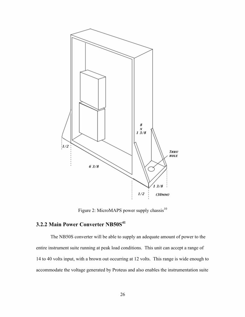
available. A basic diagram of the size of the MicroMAPS power supply is shown in
Figure 2.
An alternative solution for the MicroMAPS instrument power supply is the
NB45T triple output DC-DC converter (section 3.2.4) offered by Martek Power. This
unit can provide the necessary power and regulation required to efficiently run the in-
strument and should be coupled with an additional NBF50 EMI filter.
26
Figure 2: MicroMAPS power supply chassis10
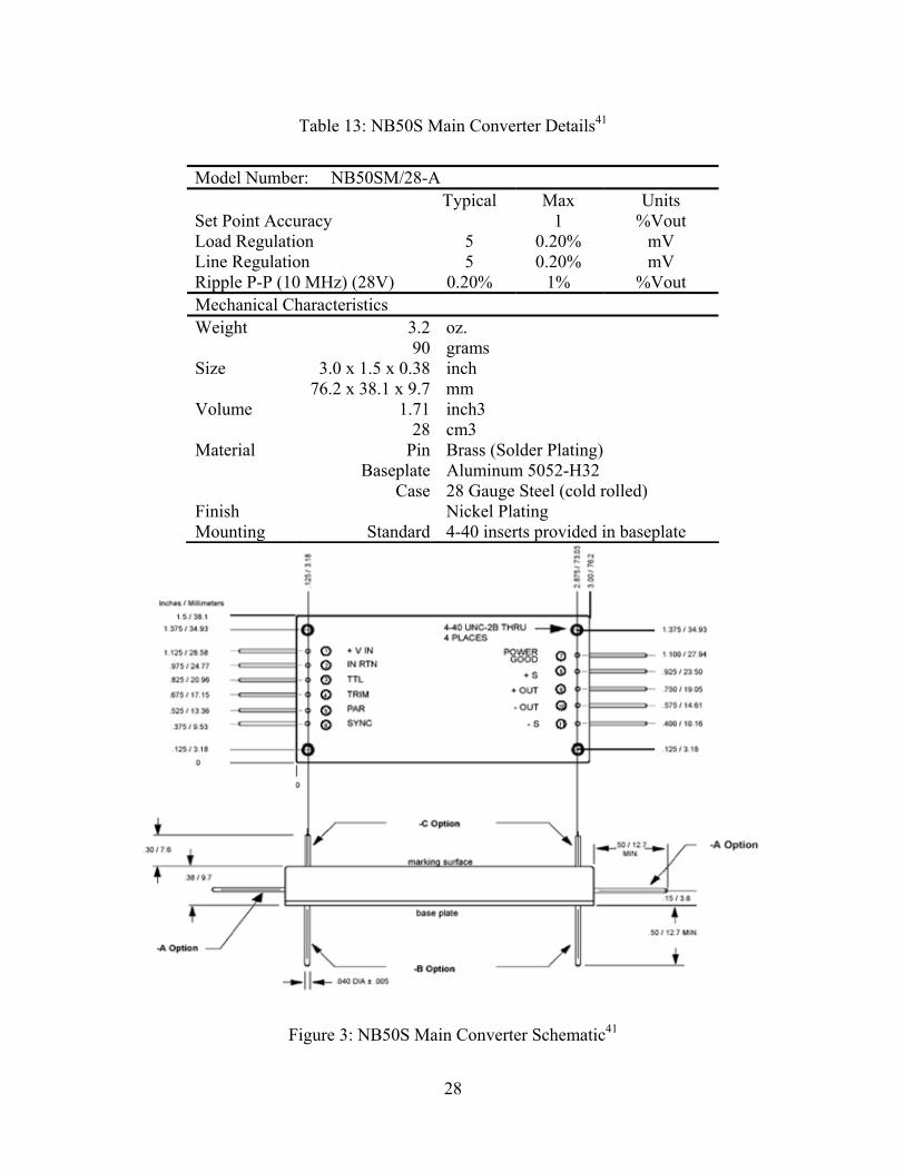
3.2.2 Main Power Converter NB50S41
The NB50S converter will be able to supply an adequate amount of power to the
entire instrument suite running at peak load conditions. This unit can accept a range of
14 to 40 volts input, with a brown out occurring at 12 volts. This range is wide enough to
accommodate the voltage generated by Proteus and also enables the instrumentation suite

27
to be used on any other system within the input range of the unit. Additional details of
the converter are shown in Table 13. Figure 3 shows a detailed schematic of the NB50S.
There is a heatsink attached to the bottom of the module. The unit is attached to
the main-plate through four 4-40 inserts. There are different options for the arrangements
of the input and output pins. The ideal choice for this system is option A: pins out of the
side of the unit. This configuration should be used for all modules requiring this option.
The input leads to this unit should be supplemented with an NBF50 EMI filter
(section 3.2.5). In addition, two fuses should be connected in parallel to the positive lead
of the NBF50 EMI filter. These fuses are slo-blow type MDX or equivalent fuses with a
minimum current rating of 5 amps and a voltage rating of at least 125V. The output con-
nections should also be wired into the positive and negative S pins, as shown in Figure 7.
These pins enable remote sensing of voltage to compensate for voltage loss due to wiring.
This feature is not necessary but must be disabled as described.
28
Table 13: NB50S Main Converter Details41
Model Number: NB50SM/28-A Typical Max Units Set Point Accuracy 1 %Vout Load Regulation 5 0.20% mV Line Regulation 5 0.20% mV Ripple P-P (10 MHz) (28V) 0.20% 1% %Vout Mechanical Characteristics Weight 3.2 oz. 90 grams Size 3.0 x 1.5 x 0.38 inch 76.2 x 38.1 x 9.7 mm Volume 1.71 inch3 28 cm3 Material Pin Brass (Solder Plating) Baseplate Aluminum 5052-H32 Case 28 Gauge Steel (cold rolled) Finish Nickel Plating Mounting Standard 4-40 inserts provided in baseplate
Figure 3: NB50S Main Converter Schematic41
29
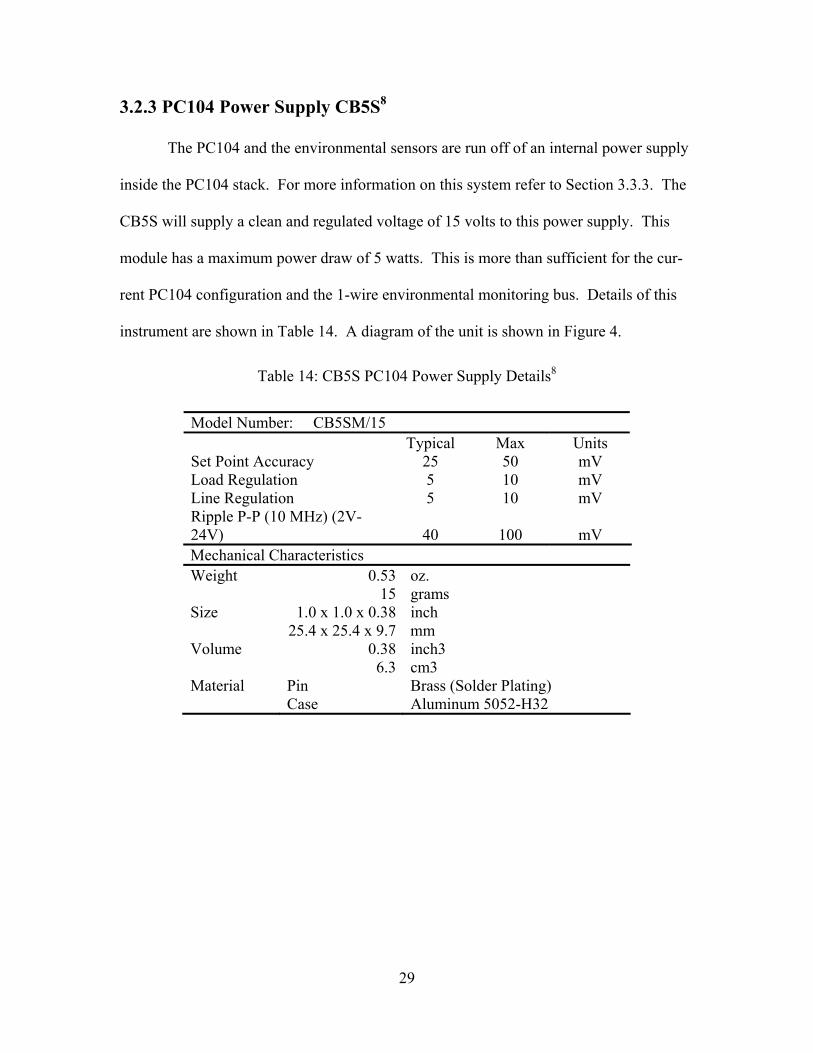
3.2.3 PC104 Power Supply CB5S8
The PC104 and the environmental sensors are run off of an internal power supply
inside the PC104 stack. For more information on this system refer to Section 3.3.3. The
CB5S will supply a clean and regulated voltage of 15 volts to this power supply. This
module has a maximum power draw of 5 watts. This is more than sufficient for the cur-
rent PC104 configuration and the 1-wire environmental monitoring bus. Details of this
instrument are shown in Table 14. A diagram of the unit is shown in Figure 4.
Table 14: CB5S PC104 Power Supply Details8
Model Number: CB5SM/15 Typical Max Units Set Point Accuracy 25 50 mV Load Regulation 5 10 mV Line Regulation 5 10 mV Ripple P-P (10 MHz) (2V-24V) 40 100 mV Mechanical Characteristics Weight 0.53 oz. 15 grams Size 1.0 x 1.0 x 0.38 inch 25.4 x 25.4 x 9.7 mm Volume 0.38 inch3 6.3 cm3 Material Pin Brass (Solder Plating) Case Aluminum 5052-H32
30
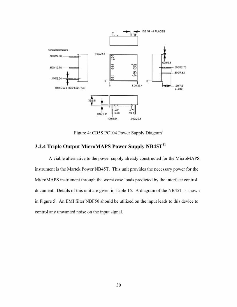
Figure 4: CB5S PC104 Power Supply Diagram8
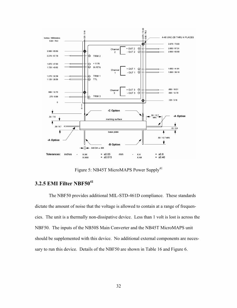
3.2.4 Triple Output MicroMAPS Power Supply NB45T41
A viable alternative to the power supply already constructed for the MicroMAPS
instrument is the Martek Power NB45T. This unit provides the necessary power for the
MicroMAPS instrument through the worst case loads predicted by the interface control
document. Details of this unit are given in Table 15. A diagram of the NB45T is shown
in Figure 5. An EMI filter NBF50 should be utilized on the input leads to this device to
control any unwanted noise on the input signal.
31
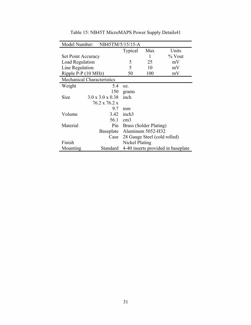
Table 15: NB45T MicroMAPS Power Supply Details41
Model Number: NB45TM/5/15/15-A Typical Max Units Set Point Accuracy 1 % Vout Load Regulation 5 25 mV Line Regulation 5 10 mV Ripple P-P (10 MHz) 50 100 mV Mechanical Characteristics Weight 5.4 oz. 150 grams Size 3.0 x 3.0 x 0.38 inch
76.2 x 76.2 x
9.7 mm Volume 3.42 inch3 56.1 cm3 Material Pin Brass (Solder Plating) Baseplate Aluminum 5052-H32 Case 28 Gauge Steel (cold rolled) Finish Nickel Plating Mounting Standard 4-40 inserts provided in baseplate
32
Figure 5: NB45T MicroMAPS Power Supply41
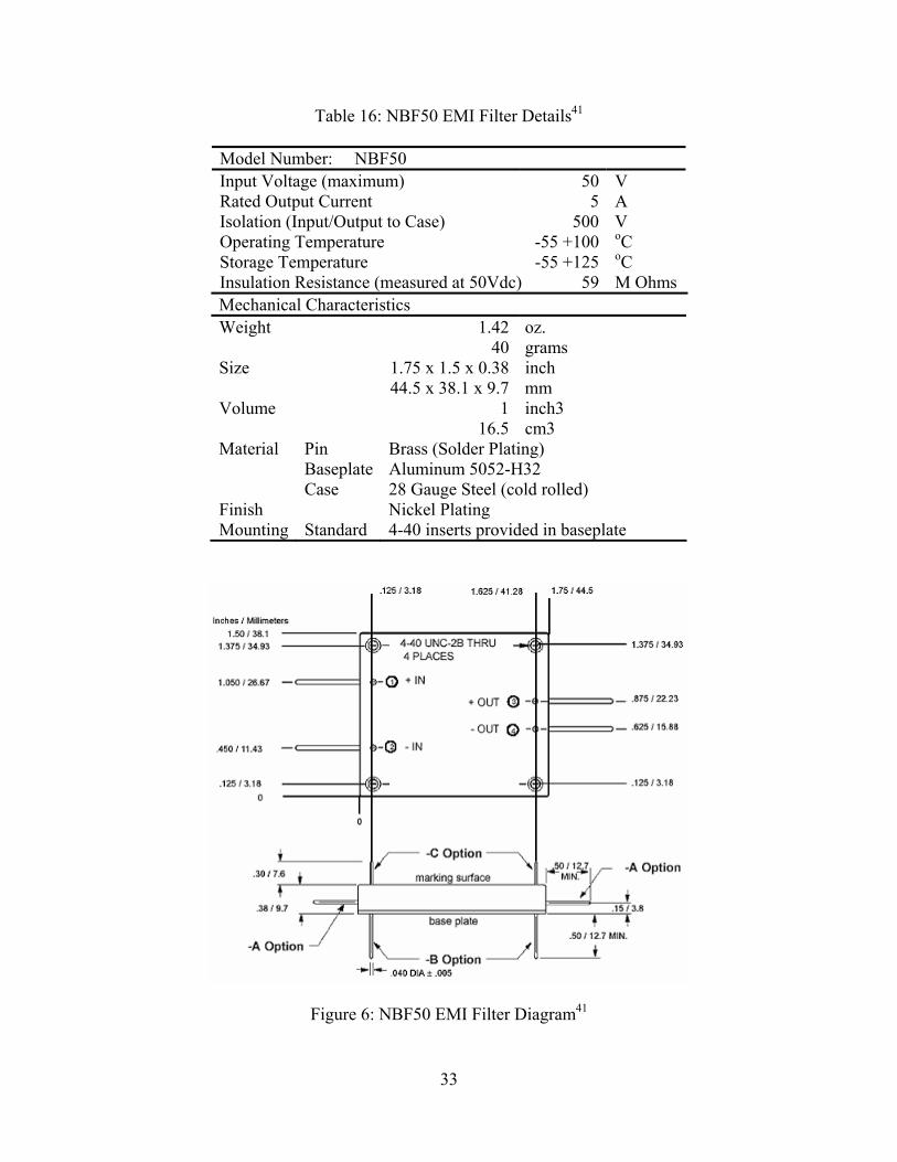
3.2.5 EMI Filter NBF5041
The NBF50 provides additional MIL-STD-461D compliance. These standards
dictate the amount of noise that the voltage is allowed to contain at a range of frequen-
cies. The unit is a thermally non-dissipative device. Less than 1 volt is lost is across the
NBF50. The inputs of the NB50S Main Converter and the NB45T MicroMAPS unit
should be supplemented with this device. No additional external components are neces-
sary to run this device. Details of the NBF50 are shown in Table 16 and Figure 6.
33
Table 16: NBF50 EMI Filter Details41
Model Number: NBF50 Input Voltage (maximum) 50 V Rated Output Current 5 A Isolation (Input/Output to Case) 500 V Operating Temperature -55 +100 oC Storage Temperature -55 +125 oC Insulation Resistance (measured at 50Vdc) 59 M Ohms Mechanical Characteristics Weight 1.42 oz. 40 grams Size 1.75 x 1.5 x 0.38 inch 44.5 x 38.1 x 9.7 mm Volume 1 inch3 16.5 cm3 Material Pin Brass (Solder Plating) Baseplate Aluminum 5052-H32 Case 28 Gauge Steel (cold rolled) Finish Nickel Plating Mounting Standard 4-40 inserts provided in baseplate
Figure 6: NBF50 EMI Filter Diagram41
34
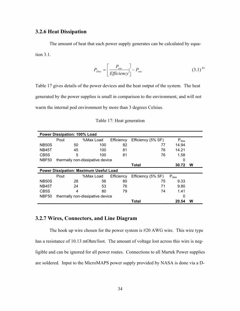
3.2.6 Heat Dissipation
The amount of heat that each power supply generates can be calculated by equa-
tion 3.1.
outout
Diss PEfficiency
PP −
= (3.1) 41
Table 17 gives details of the power devices and the heat output of the system. The heat
generated by the power supplies is small in comparison to the environment, and will not
warm the internal pod environment by more than 3 degrees Celsius.
Table 17: Heat generation
Power Dissipation: 100% Load Pout %Max Load Efficiency Efficiency (5% SF) Pdiss NB50S 50 100 82 77 14.94 NB45T 45 100 81 76 14.21 CB5S 5 100 81 76 1.58 NBF50 thermally non-dissipative device 0 Total 30.72 W Power Dissipation: Maximum Useful Load Pout %Max Load Efficiency Efficiency (5% SF) Pdiss NB50S 28 56 80 75 9.33 NB45T 24 53 76 71 9.80 CB5S 4 80 79 74 1.41 NBF50 thermally non-dissipative device 0 Total 20.54 W
3.2.7 Wires, Connectors, and Line Diagram
The hook up wire chosen for the power system is #20 AWG wire. This wire type
has a resistance of 10.13 mOhm/foot. The amount of voltage lost across this wire is neg-
ligible and can be ignored for all power routes. Connections to all Martek Power supplies
are soldered. Input to the MicroMAPS power supply provided by NASA is done via a D-
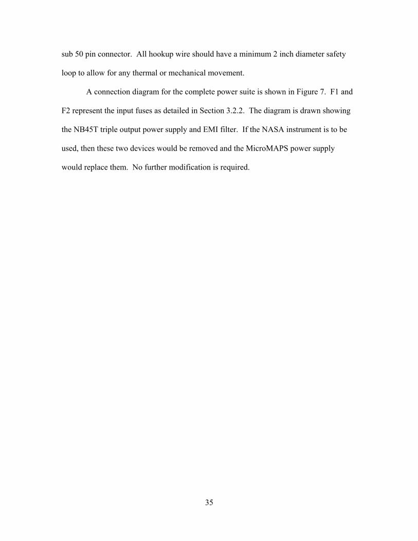
35
sub 50 pin connector. All hookup wire should have a minimum 2 inch diameter safety
loop to allow for any thermal or mechanical movement.
A connection diagram for the complete power suite is shown in Figure 7. F1 and
F2 represent the input fuses as detailed in Section 3.2.2. The diagram is drawn showing
the NB45T triple output power supply and EMI filter. If the NASA instrument is to be
used, then these two devices would be removed and the MicroMAPS power supply
would replace them. No further modification is required.
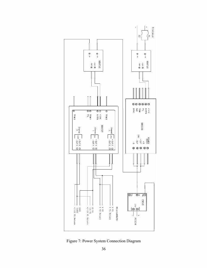
36
Figure 7: Power System Connection Diagram
37
3.3 Data Acquisition
The MicroMAPS instrument and environmental monitoring suite export data
which needs to be recorded. In addition, certain flight characteristics will also need to be
recorded: velocity, position, altitude, attitude, external environmental conditions, and
flight time. The Proteus aircraft exports this data to any payloads that request it, elimi-
nating the need for subsystems such as GPS. This data must be coordinated with the Mi-
croMAPS data in real time. The following section describes the hardware integration of
this system.
3.3.1 Computer55
The computer form factor chosen is the PC104. This compact device allows for
efficient operation in terms of electrical, mechanical, and digital data acquisition. The
PC104 had been widely adopted in the aviation and space industry. The PC104 is a reli-
able data acquisition choice and is stable in a multitude of environments.
3.3.2 CPU Board
The CPU board chosen for the MicroMAPS data acquisition and collection sys-
tem is the MZ104+ ZFx86 board. Integrated within the board is a dual Intel 82559ER
10/100 BaseT fast Ethernet connector, two 16550-compatible RS232 serial ports with
baud rates of up to 115.2 K baud, one IDE channel supporting up to two devices, dual
USB 1.1 ports, and one enhanced bidirectional parallel port. The ports for all of these
integrated systems lie on the included utility interface card. The computer will be
equipped with a 64 megabyte dimm of SDRAM which shall be purchased separately.
The chosen operating system was Linux, which shall be run from the Solid State Flash
Storage. Operating at a CPU frequency of 100 MHz with 64 megabytes of SDRAM the
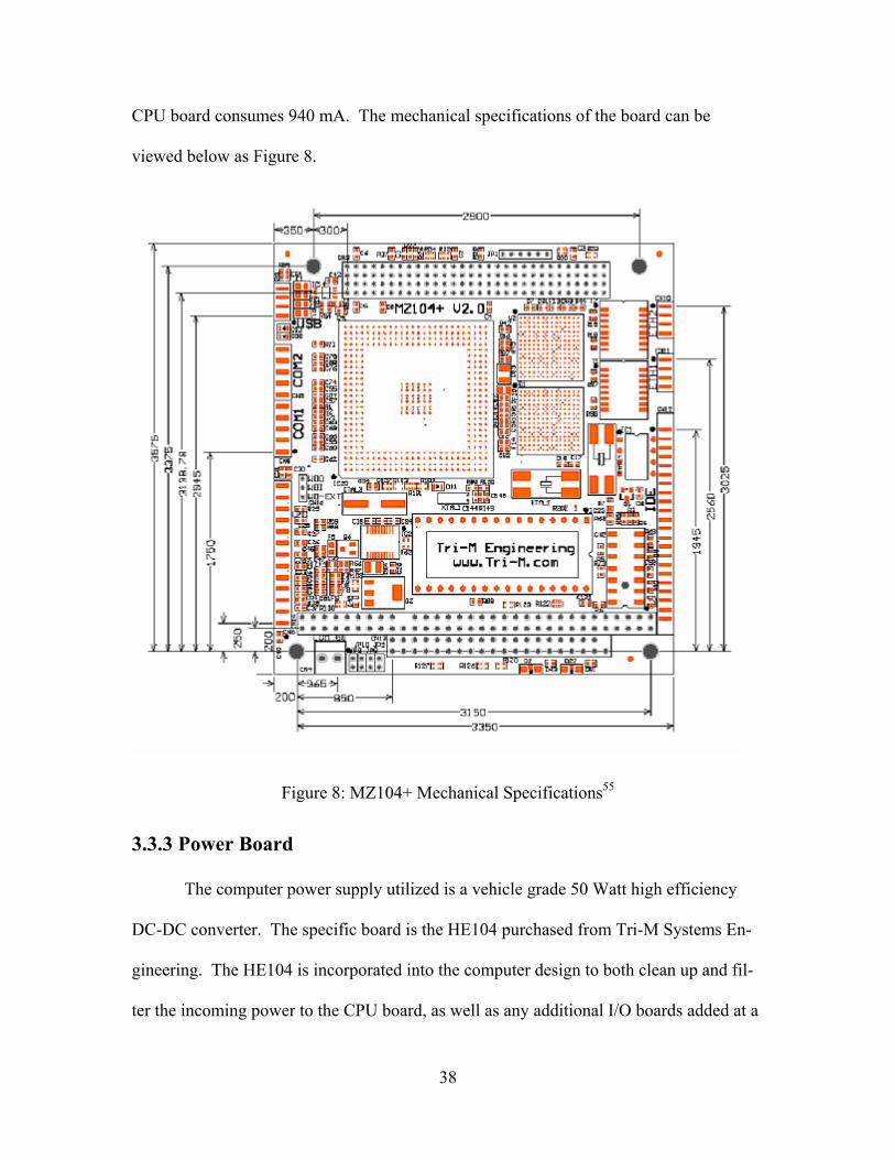
38
CPU board consumes 940 mA. The mechanical specifications of the board can be
viewed below as Figure 8.
Figure 8: MZ104+ Mechanical Specifications55
3.3.3 Power Board
The computer power supply utilized is a vehicle grade 50 Watt high efficiency
DC-DC converter. The specific board is the HE104 purchased from Tri-M Systems En-
gineering. The HE104 is incorporated into the computer design to both clean up and fil-
ter the incoming power to the CPU board, as well as any additional I/O boards added at a
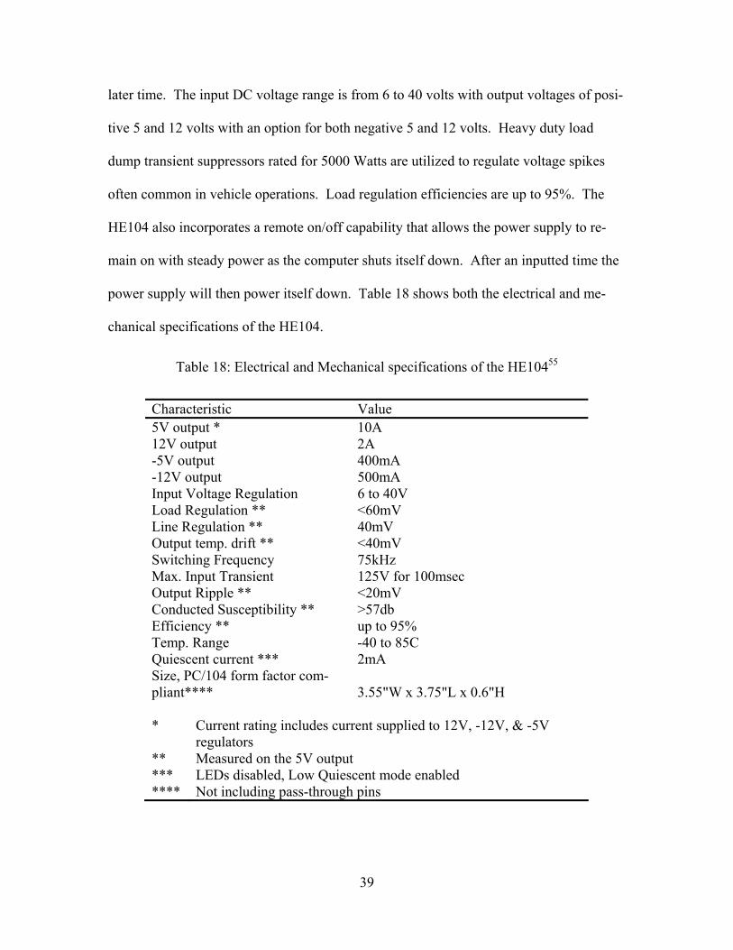
39
later time. The input DC voltage range is from 6 to 40 volts with output voltages of posi-
tive 5 and 12 volts with an option for both negative 5 and 12 volts. Heavy duty load
dump transient suppressors rated for 5000 Watts are utilized to regulate voltage spikes
often common in vehicle operations. Load regulation efficiencies are up to 95%. The
HE104 also incorporates a remote on/off capability that allows the power supply to re-
main on with steady power as the computer shuts itself down. After an inputted time the
power supply will then power itself down. Table 18 shows both the electrical and me-
chanical specifications of the HE104.
Table 18: Electrical and Mechanical specifications of the HE10455
Characteristic Value 5V output * 10A 12V output 2A -5V output 400mA -12V output 500mA Input Voltage Regulation 6 to 40V Load Regulation ** <60mV Line Regulation ** 40mV Output temp. drift ** <40mV Switching Frequency 75kHz Max. Input Transient 125V for 100msec Output Ripple ** <20mV Conducted Susceptibility ** >57db Efficiency ** up to 95% Temp. Range -40 to 85C Quiescent current *** 2mA Size, PC/104 form factor com-pliant**** 3.55"W x 3.75"L x 0.6"H * Current rating includes current supplied to 12V, -12V, & -5V
regulators ** Measured on the 5V output *** LEDs disabled, Low Quiescent mode enabled **** Not including pass-through pins
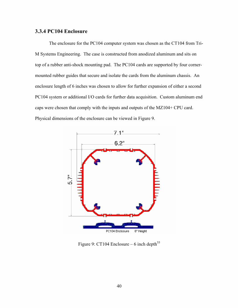
40
3.3.4 PC104 Enclosure
The enclosure for the PC104 computer system was chosen as the CT104 from Tri-
M Systems Engineering. The case is constructed from anodized aluminum and sits on
top of a rubber anti-shock mounting pad. The PC104 cards are supported by four corner-
mounted rubber guides that secure and isolate the cards from the aluminum chassis. An
enclosure length of 6 inches was chosen to allow for further expansion of either a second
PC104 system or additional I/O cards for further data acquisition. Custom aluminum end
caps were chosen that comply with the inputs and outputs of the MZ104+ CPU card.
Physical dimensions of the enclosure can be viewed in Figure 9.
Figure 9: CT104 Enclosure – 6 inch depth55
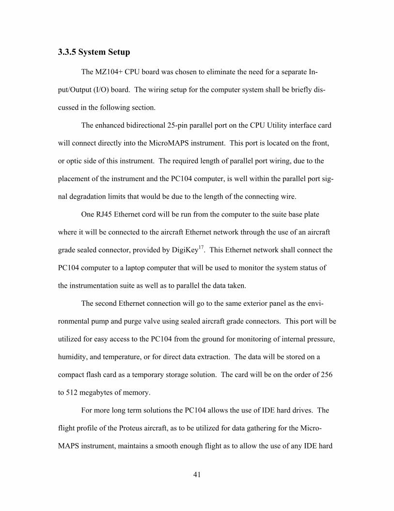
41
3.3.5 System Setup
The MZ104+ CPU board was chosen to eliminate the need for a separate In-
put/Output (I/O) board. The wiring setup for the computer system shall be briefly dis-
cussed in the following section.
The enhanced bidirectional 25-pin parallel port on the CPU Utility interface card
will connect directly into the MicroMAPS instrument. This port is located on the front,
or optic side of this instrument. The required length of parallel port wiring, due to the
placement of the instrument and the PC104 computer, is well within the parallel port sig-
nal degradation limits that would be due to the length of the connecting wire.
One RJ45 Ethernet cord will be run from the computer to the suite base plate
where it will be connected to the aircraft Ethernet network through the use of an aircraft
grade sealed connector, provided by DigiKey17. This Ethernet network shall connect the
PC104 computer to a laptop computer that will be used to monitor the system status of
the instrumentation suite as well as to parallel the data taken.
The second Ethernet connection will go to the same exterior panel as the envi-
ronmental pump and purge valve using sealed aircraft grade connectors. This port will be
utilized for easy access to the PC104 from the ground for monitoring of internal pressure,
humidity, and temperature, or for direct data extraction. The data will be stored on a
compact flash card as a temporary storage solution. The card will be on the order of 256
to 512 megabytes of memory.
For more long term solutions the PC104 allows the use of IDE hard drives. The
flight profile of the Proteus aircraft, as to be utilized for data gathering for the Micro-
MAPS instrument, maintains a smooth enough flight as to allow the use of any IDE hard

42
drive for mass storage if necessary. The G-loads as experienced by the pod are under the
failure loads of a normal off the shelf IDE hard drive. Up to two hard drives can be con-
nected in series through the IDE interface. One of the RS232 9-pin serial ports shall be
used to take the outside data from the networked flight computer to correlate with the in-
strumentation data. The two samples of data will be connected through a time stamp.
The second RS232 9-pin serial port shall be connected to the 1-wire bus card and from
this card a single RJ11 telephone cord will be placed around the instrument suite that will
contain the internal environmental telemetry sensors. This card and the associated sen-
sors are discussed in more depth in the environmental section.
3.4 Environmental Monitoring System
Through a joint effort by Virginia Tech and Virginia Space Grant Consortium an
environmental control system was developed for the safe and successful operation of the
MicroMAPS instrument and all other components. The following internal pod conditions
were established for the optimal performance of the MicroMAPS instrument: the internal
pod temperature will not be regulated since MicroMAPS performs better in a cold envi-
ronment, and humidity shall be kept at or near zero percent in order to minimize conden-
sation.
3.4.1 1-Wire® Network14
The 1-Wire® net, sometimes referred to as a MicroLAN, is a low cost bus based
on a PC or microcontroller communicating digitally over a twisted pair cable with 1-
Wire® devices. The system consists of three main elements: a bus master with controlling
software, the wiring and associated connectors, and 1-Wire® devices. Each device con-
nected on the 1-Wire® net is encoded with a 64-bit serial code unique to each device so
43
that is can be called up by the bus master. In order to achieve maximum performance,
CAT 5 UTP (unshielded twisted pair) cable is recommended for use in routing the 1-
Wire® net. Power is provided to the 1-Wire® net over the same line used for communica-
tion and ranges from 3.5 to 5 volts.
It was determined that the internal pod temperature would not be regulated, but
monitored using a number of 1-Wire® Digital Thermometers developed by Dallas Semi-
conductor. The DS18S20 1-Wire® Digital Thermometer measures temperatures from
-55°C to +125°C (-67°F to +257°F) and has an accuracy of ±0.5°C from -10°C to
+85°C14. Temperatures inside the pod during the entire mission profile will vary from
+50°C on the ground to -10°C at cruise altitude making the DS18S20 a perfect choice for
temperature observations.
Figure 10: DS18S20 1-Wire® Digital Temperature Sensor14
Humidity and condensation inside the pod will be controlled by a pump and purge
system similar to the model currently used with the NAST-I experiment on the Proteus
aircraft. The system will pump UHP (ultra high pure) nitrogen at 5 PSI into the pod re-
sulting in a dry environment with humidity at or near zero percent. Internal pod humidity
will be measured using the HMP-2001S Digital Humidity Sensor developed by Point Six,
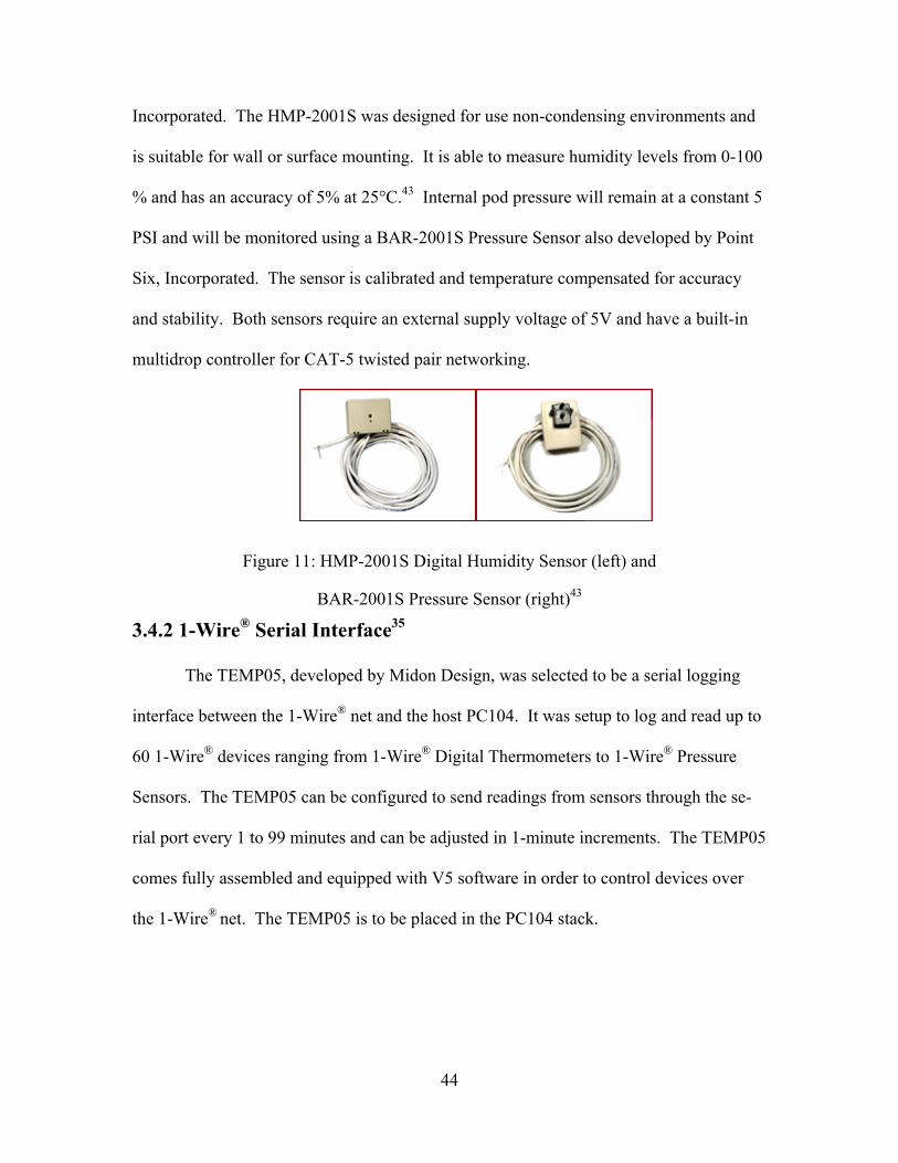
44
Incorporated. The HMP-2001S was designed for use non-condensing environments and
is suitable for wall or surface mounting. It is able to measure humidity levels from 0-100
% and has an accuracy of 5% at 25°C.43 Internal pod pressure will remain at a constant 5
PSI and will be monitored using a BAR-2001S Pressure Sensor also developed by Point
Six, Incorporated. The sensor is calibrated and temperature compensated for accuracy
and stability. Both sensors require an external supply voltage of 5V and have a built-in
multidrop controller for CAT-5 twisted pair networking.
Figure 11: HMP-2001S Digital Humidity Sensor (left) and
BAR-2001S Pressure Sensor (right)43
3.4.2 1-Wire® Serial Interface35
The TEMP05, developed by Midon Design, was selected to be a serial logging
interface between the 1-Wire® net and the host PC104. It was setup to log and read up to
60 1-Wire® devices ranging from 1-Wire® Digital Thermometers to 1-Wire® Pressure
Sensors. The TEMP05 can be configured to send readings from sensors through the se-
rial port every 1 to 99 minutes and can be adjusted in 1-minute increments. The TEMP05
comes fully assembled and equipped with V5 software in order to control devices over
the 1-Wire® net. The TEMP05 is to be placed in the PC104 stack.
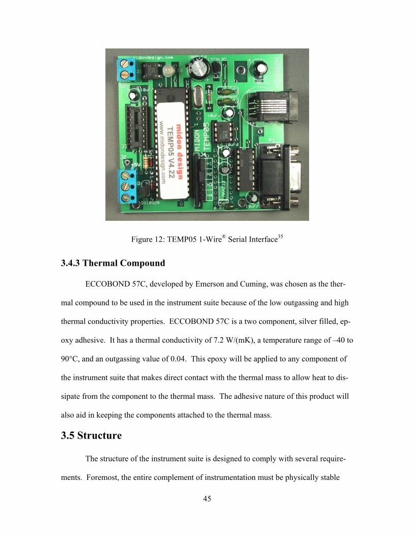
45
Figure 12: TEMP05 1-Wire® Serial Interface35
3.4.3 Thermal Compound
ECCOBOND 57C, developed by Emerson and Cuming, was chosen as the ther-
mal compound to be used in the instrument suite because of the low outgassing and high
thermal conductivity properties. ECCOBOND 57C is a two component, silver filled, ep-
oxy adhesive. It has a thermal conductivity of 7.2 W/(mK), a temperature range of –40 to
90°C, and an outgassing value of 0.04. This epoxy will be applied to any component of
the instrument suite that makes direct contact with the thermal mass to allow heat to dis-
sipate from the component to the thermal mass. The adhesive nature of this product will
also aid in keeping the components attached to the thermal mass.
3.5 Structure
The structure of the instrument suite is designed to comply with several require-
ments. Foremost, the entire complement of instrumentation must be physically stable
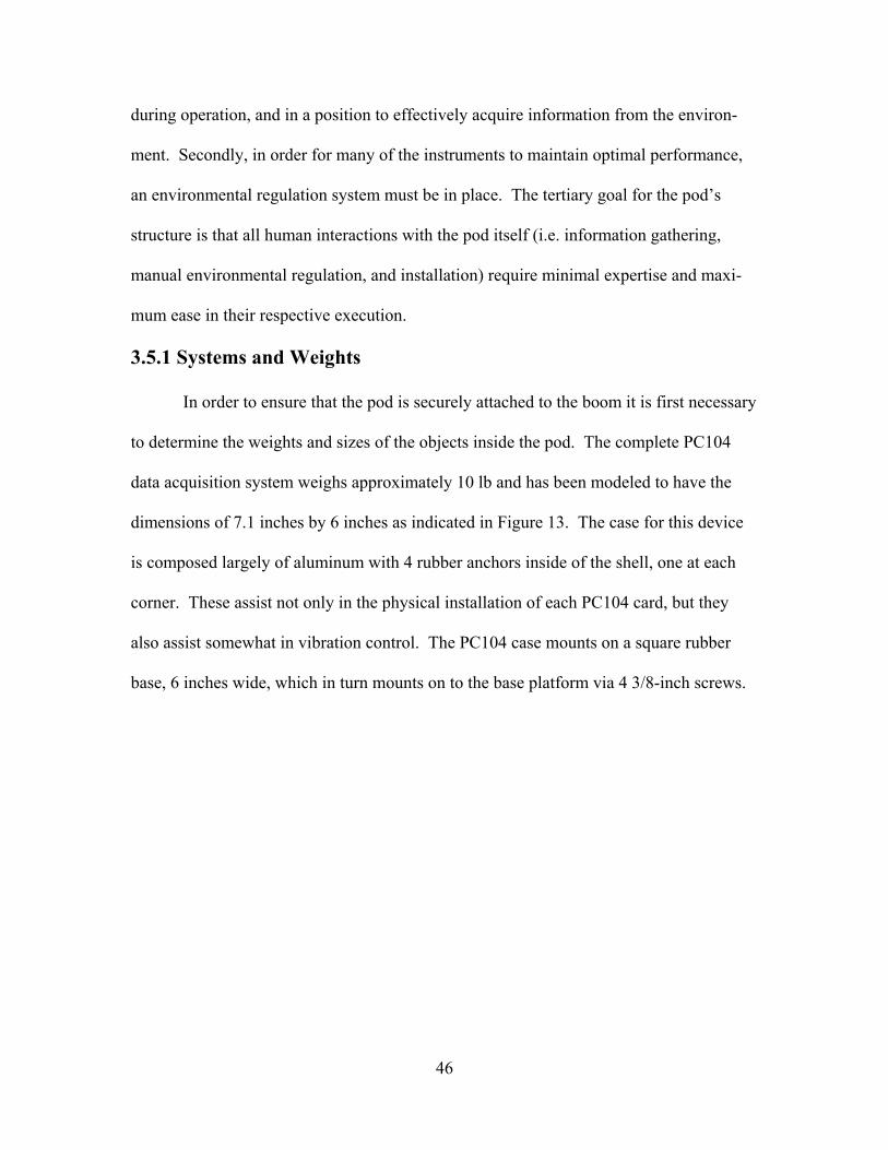
46
during operation, and in a position to effectively acquire information from the environ-
ment. Secondly, in order for many of the instruments to maintain optimal performance,
an environmental regulation system must be in place. The tertiary goal for the pod’s
structure is that all human interactions with the pod itself (i.e. information gathering,
manual environmental regulation, and installation) require minimal expertise and maxi-
mum ease in their respective execution.
3.5.1 Systems and Weights
In order to ensure that the pod is securely attached to the boom it is first necessary
to determine the weights and sizes of the objects inside the pod. The complete PC104
data acquisition system weighs approximately 10 lb and has been modeled to have the
dimensions of 7.1 inches by 6 inches as indicated in Figure 13. The case for this device
is composed largely of aluminum with 4 rubber anchors inside of the shell, one at each
corner. These assist not only in the physical installation of each PC104 card, but they
also assist somewhat in vibration control. The PC104 case mounts on a square rubber
base, 6 inches wide, which in turn mounts on to the base platform via 4 3/8-inch screws.

47
Figure 13: PC104 Exterior Casing and Mounting Base (all dimensions in inches)
The MicroMAPS instrument (Figure 14) weighs at maximum 14 lb. It has a cy-
lindrical viewing aperture 3 inches long and 1.6 inches in diameter. The rest of the in-
strument is 10 inches long, 5 ¾ inches tall and 5 3/8 inches wide. There are two 25-pin
connectors and two 15-pin connectors on the front. Four feet are attached to the base of
MicroMAPS through which 5/16-inch holes are drilled. Through these holes screws will
pass to anchor MicroMAPS to the base platform.

48
Figure 14: MicroMAPS Diagram (inches)
There are several items which comprise the power regulation and supply system.
These are discussed in detail in section 3.2 of this document. Figure 15 shows the
NBF50 EMI filter, Figure 16 shows the CB5S PC104 power supply, and Figure 17 shows
the NB50S main converter. Figure 18 shows the power supply, which is to be used ex-
clusively with MicroMAPS.
Figure 15: NBF50 Diagram (inches)
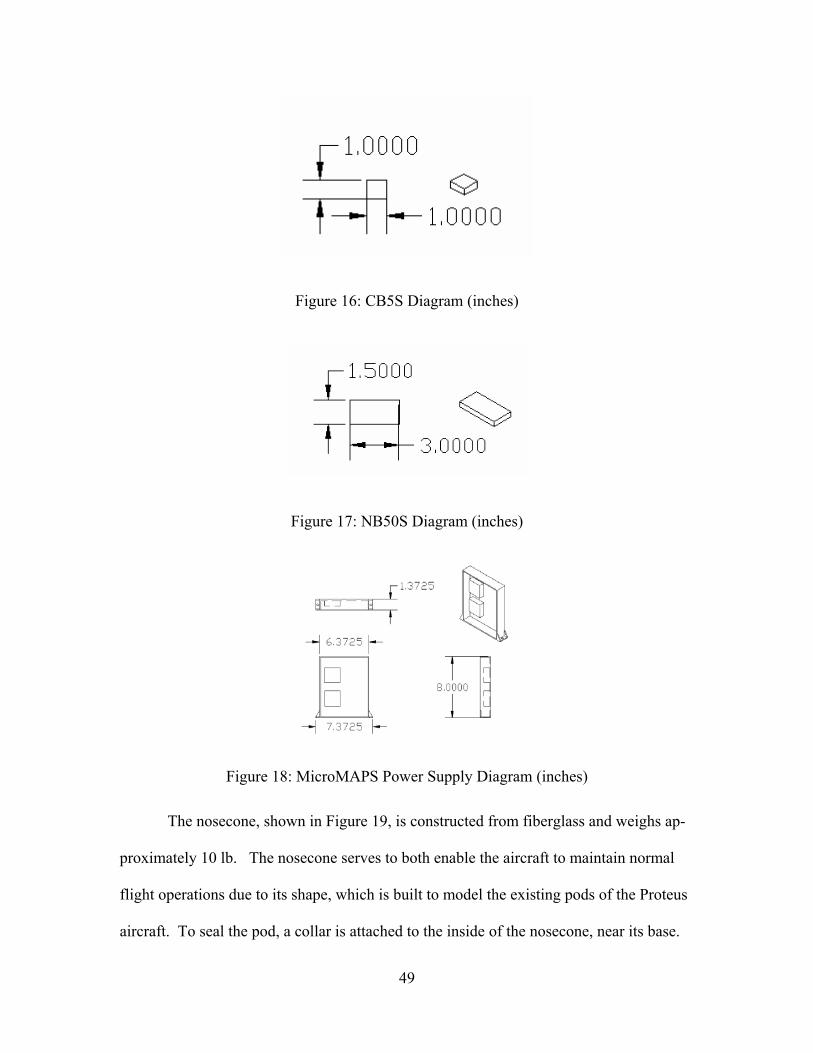
49
Figure 16: CB5S Diagram (inches)
Figure 17: NB50S Diagram (inches)
Figure 18: MicroMAPS Power Supply Diagram (inches)
The nosecone, shown in Figure 19, is constructed from fiberglass and weighs ap-
proximately 10 lb. The nosecone serves to both enable the aircraft to maintain normal
flight operations due to its shape, which is built to model the existing pods of the Proteus
aircraft. To seal the pod, a collar is attached to the inside of the nosecone, near its base.
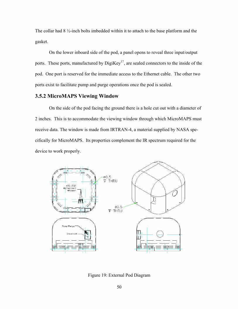
50
The collar had 8 ½-inch bolts imbedded within it to attach to the base platform and the
gasket.
On the lower inboard side of the pod, a panel opens to reveal three input/output
ports. These ports, manufactured by DigiKey17, are sealed connectors to the inside of the
pod. One port is reserved for the immediate access to the Ethernet cable. The other two
ports exist to facilitate pump and purge operations once the pod is sealed.
3.5.2 MicroMAPS Viewing Window
On the side of the pod facing the ground there is a hole cut out with a diameter of
2 inches. This is to accommodate the viewing window through which MicroMAPS must
receive data. The window is made from IRTRAN-4, a material supplied by NASA spe-
cifically for MicroMAPS. Its properties complement the IR spectrum required for the
device to work properly.
Figure 19: External Pod Diagram
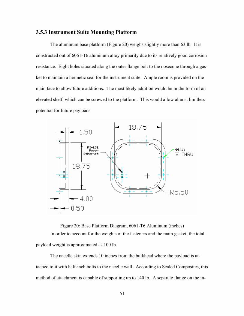
51
3.5.3 Instrument Suite Mounting Platform
The aluminum base platform (Figure 20) weighs slightly more than 63 lb. It is
constructed out of 6061-T6 aluminum alloy primarily due to its relatively good corrosion
resistance. Eight holes situated along the outer flange bolt to the nosecone through a gas-
ket to maintain a hermetic seal for the instrument suite. Ample room is provided on the
main face to allow future additions. The most likely addition would be in the form of an
elevated shelf, which can be screwed to the platform. This would allow almost limitless
potential for future payloads.
Figure 20: Base Platform Diagram, 6061-T6 Aluminum (inches)
In order to account for the weights of the fasteners and the main gasket, the total
payload weight is approximated as 100 lb.
The nacelle skin extends 10 inches from the bulkhead where the payload is at-
tached to it with half-inch bolts to the nacelle wall. According to Scaled Composites, this
method of attachment is capable of supporting up to 140 lb. A separate flange on the in-
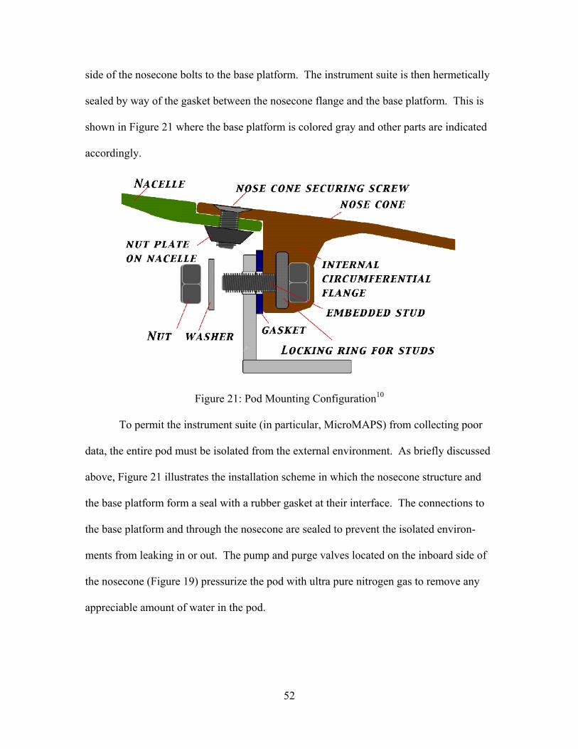
52
side of the nosecone bolts to the base platform. The instrument suite is then hermetically
sealed by way of the gasket between the nosecone flange and the base platform. This is
shown in Figure 21 where the base platform is colored gray and other parts are indicated
accordingly.
Figure 21: Pod Mounting Configuration10
To permit the instrument suite (in particular, MicroMAPS) from collecting poor
data, the entire pod must be isolated from the external environment. As briefly discussed
above, Figure 21 illustrates the installation scheme in which the nosecone structure and
the base platform form a seal with a rubber gasket at their interface. The connections to
the base platform and through the nosecone are sealed to prevent the isolated environ-
ments from leaking in or out. The pump and purge valves located on the inboard side of
the nosecone (Figure 19) pressurize the pod with ultra pure nitrogen gas to remove any
appreciable amount of water in the pod.
53
3.5.4 Installation and Configuration
The third main consideration in designing the payload installation is to ensure that
all interactions with the pod are easily carried out. The pod has a set of internal connec-
tions to the Proteus aircraft: one RS-232 interface to relay flight data to the PC104, one
Ethernet jack to relay information from the PC104 to the on-board laptop computer, and
the parasite power supply from Proteus to power the instruments.
After the physical installation of the pod, there are two sets of external connec-
tions which must be used. The first set, used prior to takeoff, is the set of pump and
purge valves which infuses the internal environment with Nitrogen gas. The second con-
nection through the nosecone is another Ethernet jack, which allows data that the PC104
has compiled to be accessed either directly on the runway or after the payload has been
physically removed from the aircraft. The installation scheme for the pod is quite simple.
The suggested method of installation is as follows:
1) All of the internal connections between the PC104, the MicroMAPS device, the 1-
wire bus, and the power supplies must be made (this is discussed in detail in sec-
tions 3.2, 3.3, and 3.4).
2) On the instrument-side of the base platform, cables are to be run from the
DigiKey sealed connectors to their respective instruments. The RS-232 and the
Ethernet cable run to the PC104 computer, the power cable runs to the NB50S
main power supply. One additional internal Ethernet cable must be run from the
PC104 to the jack on the inboard interior of the nosecone. This permits data to be
downloaded directly on the runway without removing the entire nosecone.
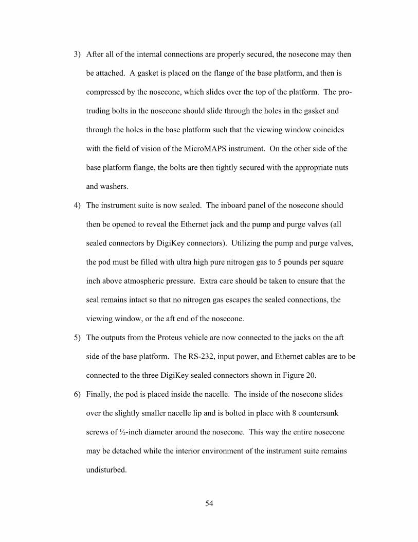
54
3) After all of the internal connections are properly secured, the nosecone may then
be attached. A gasket is placed on the flange of the base platform, and then is
compressed by the nosecone, which slides over the top of the platform. The pro-
truding bolts in the nosecone should slide through the holes in the gasket and
through the holes in the base platform such that the viewing window coincides
with the field of vision of the MicroMAPS instrument. On the other side of the
base platform flange, the bolts are then tightly secured with the appropriate nuts
and washers.
4) The instrument suite is now sealed. The inboard panel of the nosecone should
then be opened to reveal the Ethernet jack and the pump and purge valves (all
sealed connectors by DigiKey connectors). Utilizing the pump and purge valves,
the pod must be filled with ultra high pure nitrogen gas to 5 pounds per square
inch above atmospheric pressure. Extra care should be taken to ensure that the
seal remains intact so that no nitrogen gas escapes the sealed connections, the
viewing window, or the aft end of the nosecone.
5) The outputs from the Proteus vehicle are now connected to the jacks on the aft
side of the base platform. The RS-232, input power, and Ethernet cables are to be
connected to the three DigiKey sealed connectors shown in Figure 20.
6) Finally, the pod is placed inside the nacelle. The inside of the nosecone slides
over the slightly smaller nacelle lip and is bolted in place with 8 countersunk
screws of ½-inch diameter around the nosecone. This way the entire nosecone
may be detached while the interior environment of the instrument suite remains
undisturbed.
55
Chapter 4: Menelaus
4.1 Introduction
In this chapter, the aircraft design is taken from RFP requirements to final pro-
posal. The chapter is organized as follows: Request for Proposal (RFP), Selection of the
Final Design Concept; Detailed Sizing; Propulsion; Aerodynamics; Stability and Control;
Performance; Materials and Structure; Systems; Cost; and Final Proposal.
4.2 Aircraft RFP
The need for an aircraft to carry out atmospheric observation with MicroMAPS
evolved over the last three decades. In the 1970s, scientists developing chemical and
transport models for atmospheric gases identified a need for a “long term measurement
program for atmospheric CO, CH4, and OH concentrations” in the troposphere.53 In re-
sponse, large and rather crude space-based instruments, like MAPS (Measurement of
Atmospheric Pollution for Satellites), were developed and deployed. NASA’s small sat-
ellite technology initiative (SSTI) then instigated the development of a second-generation
instrument. The motivation for the new design was to make the instrument smaller,
cheaper, and more useful. The result is MicroMAPS.
MicroMAPS was originally designed as a space-based platform, but the scientists
at NASA Langley Research Center (LaRC) realized that operating the instrument on-
board an aircraft could offer excellent data gathering opportunities. The aircraft platform
affords several advantages over the satellite platform. These advantages include lower
cost, more detailed local data, improved geophysical data, and the capacity to respond to
56
and track specific emissions episodes, amass detailed column distribution data, and fly in
multi-aircraft, multi-instrument coordinated missions.
The cost of launching a satellite of this size into low earth orbit (LEO) is on the
order of ten to twenty million dollars. For a fraction of that cost, MicroMAPS could be
operated in atmospheric flight, taking advantage of the flexible mission profile an aircraft
platform offers.
Aircraft-based operation of MicroMAPS allows gathering of ultra-fine and spa-
tially varying data.12 A spacecraft in LEO has a ground speed of about 15,000 kts
(~17,000 mph) and cannot change its direction. The observational opportunities are lim-
ited to a fast-moving, fixed-swath-width, linear path that requires many orbits to pass
over the same location on earth twice. Onboard an aircraft, the instrument can gather
much finer data due to the relatively slow ground speed. The ground track is not limited
to one direction, but is determined at the scientists’ discretion.
MicroMAPS can gather better geophysical data from the relatively low opera-
tional altitude onboard an aircraft than it can from LEO.12 The instrument uses earth-
generated infrared radiation (IR) to detect the absorption line spectra of trace gases in the
atmosphere. This radiation, like all electromagnetic radiation, decreases in strength in
proportion to the square of the distance from its source. The IR signal at high altitude,
atmospheric flight (~65,000 ft) will be about 350 times stronger than that available at
LEO altitudes.
An aircraft-based instrument allows scientists to respond to specific emissions
episodes and to track their effect on atmospheric chemistry.12 These events include natu-
ral sources of gases, such as a volcanic eruption, and anthropogenic sources, such as
57
biomass burning caused by deforestation. A spacecraft, constrained by its orbit, cannot
respond to specific episodes.
With its capacity to operate the instrument at various altitudes, an aircraft plat-
form allows MicroMAPS to gather extensive altitude profiling data.12 Column distribu-
tion measurements can be made from LEO, but the detail of the data is limited by the
spacecraft’s fixed altitude. An aircraft can fly any altitude schedule the scientists wish,
giving them more options for data gathering.
An aircraft-based instrument could be operated in multi-aircraft coordinated mis-
sions. These coordinated flights could provide multi-platform validation, enhanced
measurement from combined instruments, a wider effective swath, and a larger coverage
zone.12 Each aircraft could be fitted with a MicroMAPS instrument or with a different
instrument. This type of coordinated data gathering offers the scientists a great deal of
flexibility with their science goals.
An aircraft platform is desirable for the mission flexibility and unique data gather-
ing opportunities it affords the scientists. To maximize these benefits, the requirements
of the RFP have been developed. They are stated and explained below.
7) The cruise altitude shall be no less than 60,000 ft [65,000]*. This altitude will
place the instrument far enough above the troposphere (0 to 36,000 ft) and will
give a wide enough viewing swath to gather the desired data.
8) The maximum endurance at cruise altitude shall be no less than 36 [40] hours
without refueling. This endurance will allow tracking of specific emissions epi-
* Please note that the RFP was altered after a February 2003 meeting with Dr. Vickie Connors. The old requirements are enclosed in brackets.
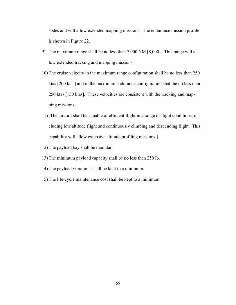
58
sodes and will allow extended mapping missions. The endurance mission profile
is shown in Figure 22.
9) The maximum range shall be no less than 7,000 NM [8,000]. This range will al-
low extended tracking and mapping missions.
10) The cruise velocity in the maximum range configuration shall be no less than 250
ktas [200 ktas] and in the maximum endurance configuration shall be no less than
250 ktas [150 ktas]. These velocities are consistent with the tracking and map-
ping missions.
11) [The aircraft shall be capable of efficient flight in a range of flight conditions, in-
cluding low altitude flight and continuously climbing and descending flight. This
capability will allow extensive altitude profiling missions.]
12) The payload bay shall be modular.
13) The minimum payload capacity shall be no less than 250 lb.
14) The payload vibrations shall be kept to a minimum.
15) The life-cycle maintenance cost shall be kept to a minimum.
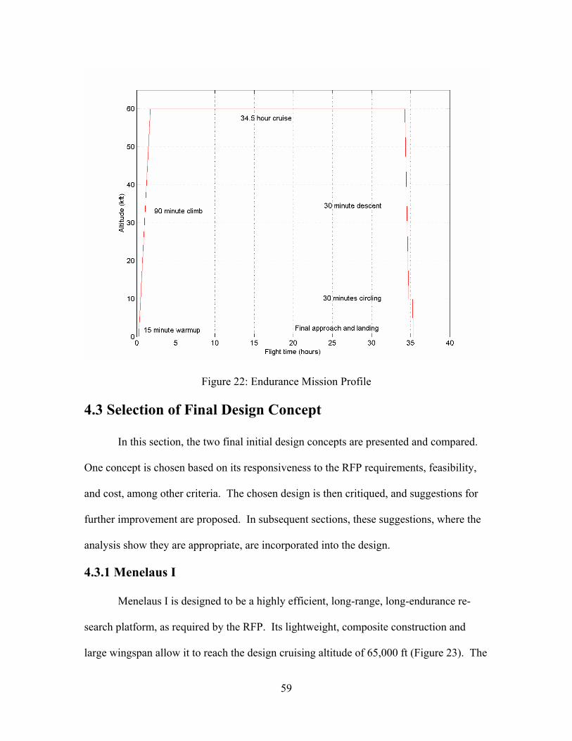
59
Figure 22: Endurance Mission Profile
4.3 Selection of Final Design Concept
In this section, the two final initial design concepts are presented and compared.
One concept is chosen based on its responsiveness to the RFP requirements, feasibility,
and cost, among other criteria. The chosen design is then critiqued, and suggestions for
further improvement are proposed. In subsequent sections, these suggestions, where the
analysis show they are appropriate, are incorporated into the design.
4.3.1 Menelaus I
Menelaus I is designed to be a highly efficient, long-range, long-endurance re-
search platform, as required by the RFP. Its lightweight, composite construction and
large wingspan allow it to reach the design cruising altitude of 65,000 ft (Figure 23). The
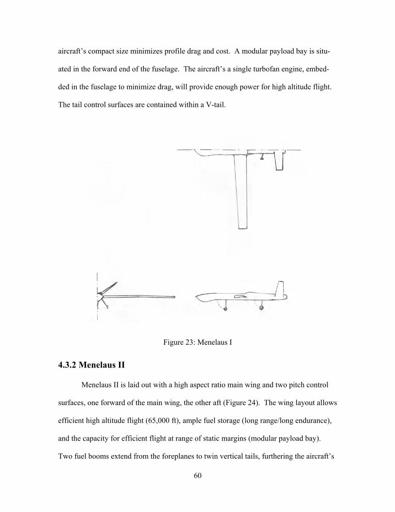
60
aircraft’s compact size minimizes profile drag and cost. A modular payload bay is situ-
ated in the forward end of the fuselage. The aircraft’s a single turbofan engine, embed-
ded in the fuselage to minimize drag, will provide enough power for high altitude flight.
The tail control surfaces are contained within a V-tail.
Figure 23: Menelaus I
4.3.2 Menelaus II
Menelaus II is laid out with a high aspect ratio main wing and two pitch control
surfaces, one forward of the main wing, the other aft (Figure 24). The wing layout allows
efficient high altitude flight (65,000 ft), ample fuel storage (long range/long endurance),
and the capacity for efficient flight at range of static margins (modular payload bay).
Two fuel booms extend from the foreplanes to twin vertical tails, furthering the aircraft’s
61
fuel capacity. The axi-symmetric fuselage nosecone is free to rotate around its axis, al-
lowing a control system to maintain nadir pointing during a turn. A small turbofan en-
gine drives the aircraft. The air intake is on top of the fuselage, well aft. This system of-
fers excellent efficiency at high altitude and meets the cruise speed requirement (250
ktas). If later trade studies show a turboprop or a piston motor-driven propeller to be
more appropriate, this concept could be modified to accommodate the change easily.
Figure 24: Menelaus II
4.3.3 The Decision and Suggested Changes
The decision matrix in Table 19 is used to decide between the two concepts. The
criteria for this decision are developed directly from the RFP and from a general consid-
eration of feasibility. Each design is then given a numerical rating with respect to each
category. The numerical scale ranges from –2 to 2, where –2 is the least desirable, 2 is
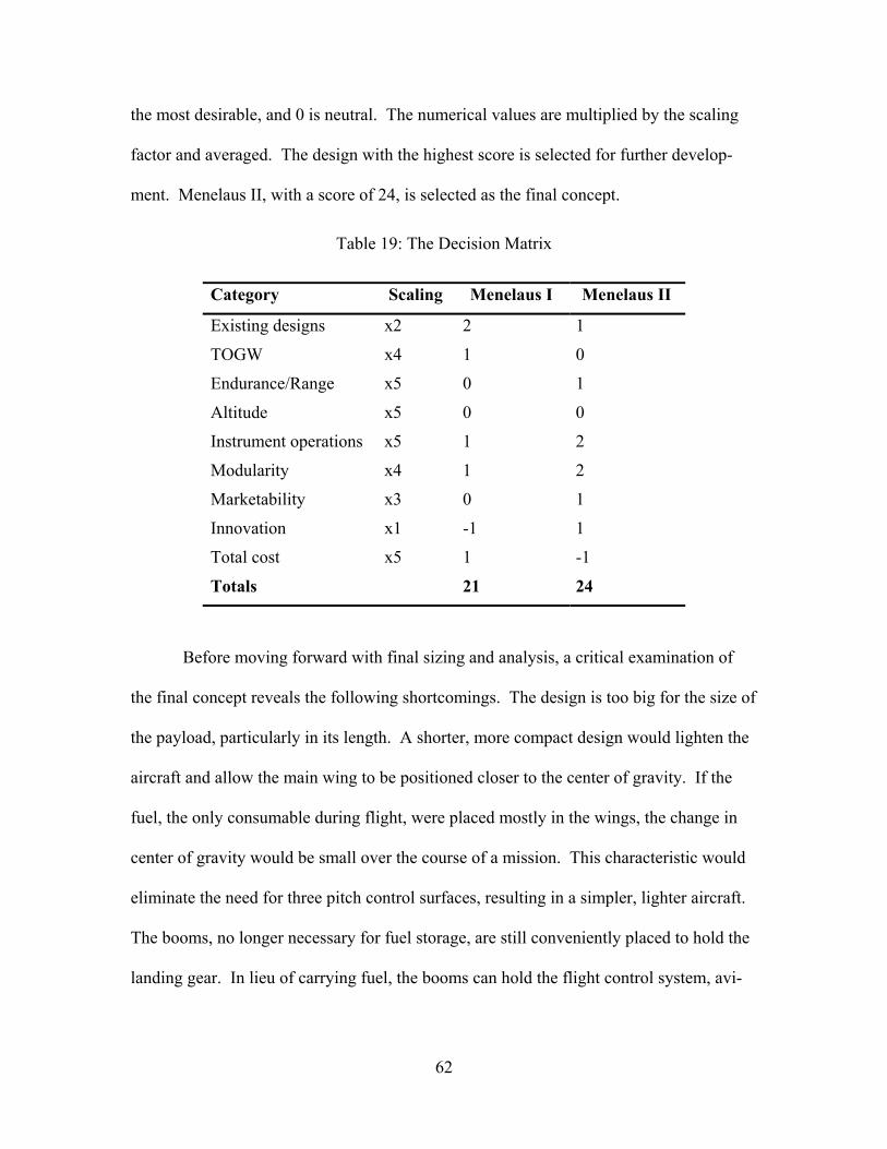
62
the most desirable, and 0 is neutral. The numerical values are multiplied by the scaling
factor and averaged. The design with the highest score is selected for further develop-
ment. Menelaus II, with a score of 24, is selected as the final concept.
Table 19: The Decision Matrix
Category Scaling Menelaus I Menelaus II
Existing designs x2 2 1
TOGW x4 1 0
Endurance/Range x5 0 1
Altitude x5 0 0
Instrument operations x5 1 2
Modularity x4 1 2
Marketability x3 0 1
Innovation x1 -1 1
Total cost x5 1 -1
Totals 21 24
Before moving forward with final sizing and analysis, a critical examination of
the final concept reveals the following shortcomings. The design is too big for the size of
the payload, particularly in its length. A shorter, more compact design would lighten the
aircraft and allow the main wing to be positioned closer to the center of gravity. If the
fuel, the only consumable during flight, were placed mostly in the wings, the change in
center of gravity would be small over the course of a mission. This characteristic would
eliminate the need for three pitch control surfaces, resulting in a simpler, lighter aircraft.
The booms, no longer necessary for fuel storage, are still conveniently placed to hold the
landing gear. In lieu of carrying fuel, the booms can hold the flight control system, avi-

63
onics, radar, and other systems, freeing space in the fuselage for the payload, fuel system,
engine, and additional fuel tanks.
The empennage design, with two vertical surfaces and a connecting horizontal
surface looks over-sized and heavy. It could be redesigned as an inverted V-tail (this tail
configuration will be referred to as an A-tail for the remainder of the report). This con-
figuration could reduce drag by decreasing the wetted surface area and could save struc-
tural weight.
These suggested changes are evaluated and implemented in the following sec-
tions.
4.4 Detailed Sizing
Before the final round of sizing is performed, the suggested changes to the design
are incorporated. The aircraft’s fuselage and tail booms are shortened. The booms’
noses are placed just forward of the main wing, and the foreplanes are eliminated. The
empennage design is changed from two vertical surfaces and a joining horizontal surface
to an A-tail, which incorporates pitch-yaw control surfaces (these surfaces will be re-
ferred to a ruddervators for the remainder of the report). The design is shown in Figure
25.

64
Figure 25: New Configuration, Including Changes Developed in Decision Process
The resulting concept is a low wing monoplane with axi-symmetric fuselage and
tail booms. The A-tail supports the ruddervators and, at its apex, a satellite communica-
tions dome. The fuel is stored primarily in the high aspect ratio wing, which is mounted
near the aircraft’s center of gravity. The tail boom noses, which extend forward of the
main wing’s leading edge, house a collision control system that will sense other aircraft
and execute tactics to avoid them autonomously. (Such a system is under development at
NASA and has been successfully tested onboard Proteus.) 39 The analysis that justifies
this configuration is developed in sections dedicated to the aircraft’s subsystems.
4.4.1 Sizing Process
Detailed sizing is accomplished using two methods. First, a detailed analysis of
data gathered from existing aircraft that meet some of the RFP requirements is per-
formed. A weighted average of the value of interest is calculated, giving more weight to
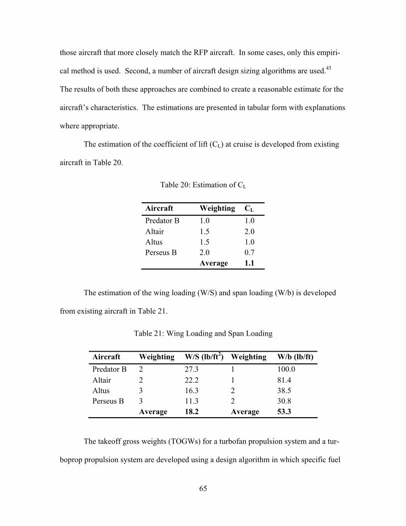
65
those aircraft that more closely match the RFP aircraft. In some cases, only this empiri-
cal method is used. Second, a number of aircraft design sizing algorithms are used.45
The results of both these approaches are combined to create a reasonable estimate for the
aircraft’s characteristics. The estimations are presented in tabular form with explanations
where appropriate.
The estimation of the coefficient of lift (CL) at cruise is developed from existing
aircraft in Table 20.
Table 20: Estimation of CL
Aircraft Weighting CL
Predator B 1.0 1.0 Altair 1.5 2.0 Altus 1.5 1.0 Perseus B 2.0 0.7 Average 1.1
The estimation of the wing loading (W/S) and span loading (W/b) is developed
from existing aircraft in Table 21.
Table 21: Wing Loading and Span Loading
Aircraft Weighting W/S (lb/ft2) Weighting W/b (lb/ft) Predator B 2 27.3 1 100.0 Altair 2 22.2 1 81.4 Altus 3 16.3 2 38.5 Perseus B 3 11.3 2 30.8 Average 18.2 Average 53.3
The takeoff gross weights (TOGWs) for a turbofan propulsion system and a tur-
boprop propulsion system are developed using a design algorithm in which specific fuel
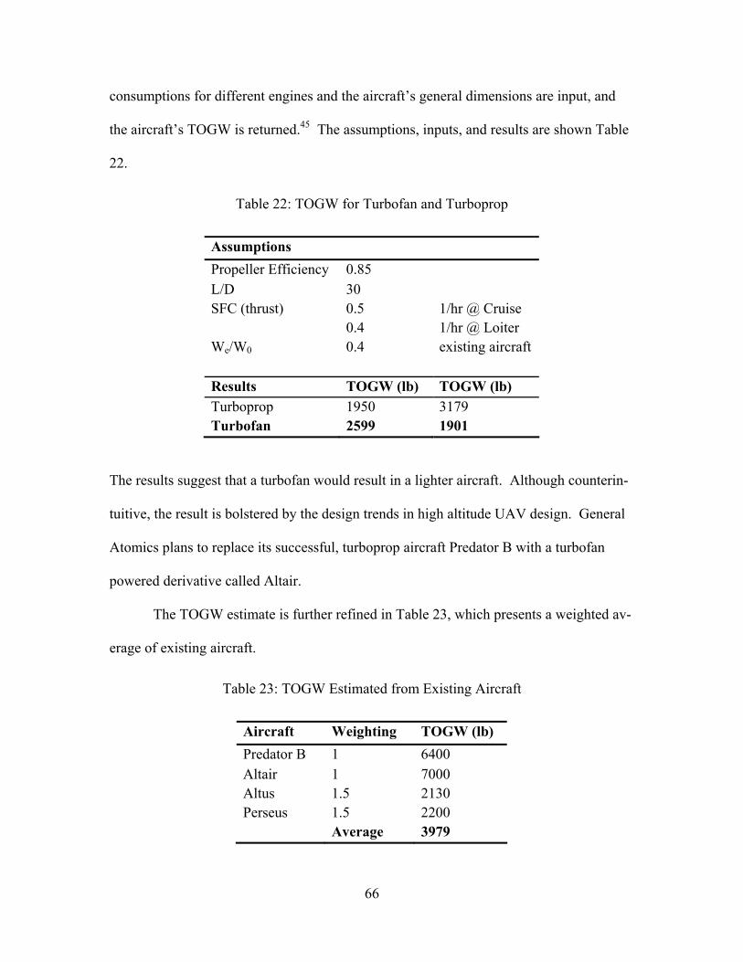
66
consumptions for different engines and the aircraft’s general dimensions are input, and
the aircraft’s TOGW is returned.45 The assumptions, inputs, and results are shown Table
22.
Table 22: TOGW for Turbofan and Turboprop
Assumptions
Propeller Efficiency 0.85 L/D 30 SFC (thrust) 0.5 1/hr @ Cruise 0.4 1/hr @ Loiter We/W0 0.4 existing aircraft Results TOGW (lb) TOGW (lb) Turboprop 1950 3179 Turbofan 2599 1901
The results suggest that a turbofan would result in a lighter aircraft. Although counterin-
tuitive, the result is bolstered by the design trends in high altitude UAV design. General
Atomics plans to replace its successful, turboprop aircraft Predator B with a turbofan
powered derivative called Altair.
The TOGW estimate is further refined in Table 23, which presents a weighted av-
erage of existing aircraft.
Table 23: TOGW Estimated from Existing Aircraft
Aircraft Weighting TOGW (lb)
Predator B 1 6400 Altair 1 7000 Altus 1.5 2130 Perseus 1.5 2200 Average 3979
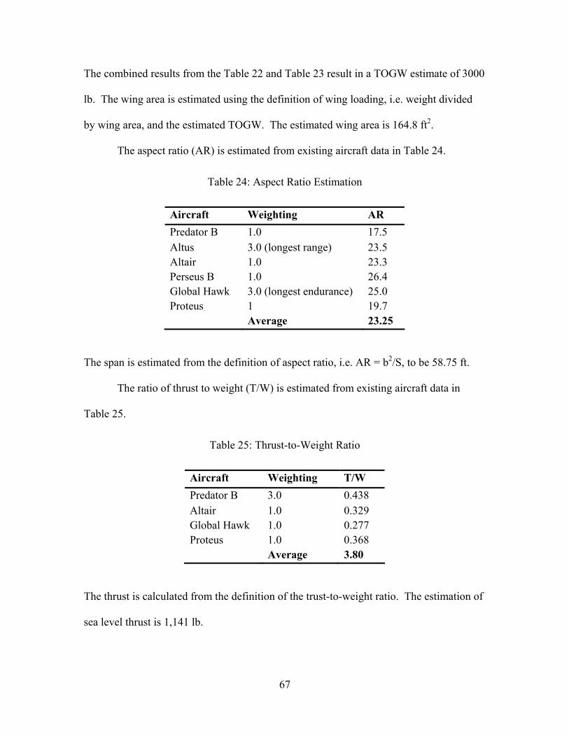
67
The combined results from the Table 22 and Table 23 result in a TOGW estimate of 3000
lb. The wing area is estimated using the definition of wing loading, i.e. weight divided
by wing area, and the estimated TOGW. The estimated wing area is 164.8 ft2.
The aspect ratio (AR) is estimated from existing aircraft data in Table 24.
Table 24: Aspect Ratio Estimation
Aircraft Weighting AR
Predator B 1.0 17.5 Altus 3.0 (longest range) 23.5 Altair 1.0 23.3 Perseus B 1.0 26.4 Global Hawk 3.0 (longest endurance) 25.0 Proteus 1 19.7 Average 23.25
The span is estimated from the definition of aspect ratio, i.e. AR = b2/S, to be 58.75 ft.
The ratio of thrust to weight (T/W) is estimated from existing aircraft data in
Table 25.
Table 25: Thrust-to-Weight Ratio
Aircraft Weighting T/W
Predator B 3.0 0.438 Altair 1.0 0.329 Global Hawk 1.0 0.277 Proteus 1.0 0.368 Average 3.80
The thrust is calculated from the definition of the trust-to-weight ratio. The estimation of
sea level thrust is 1,141 lb.
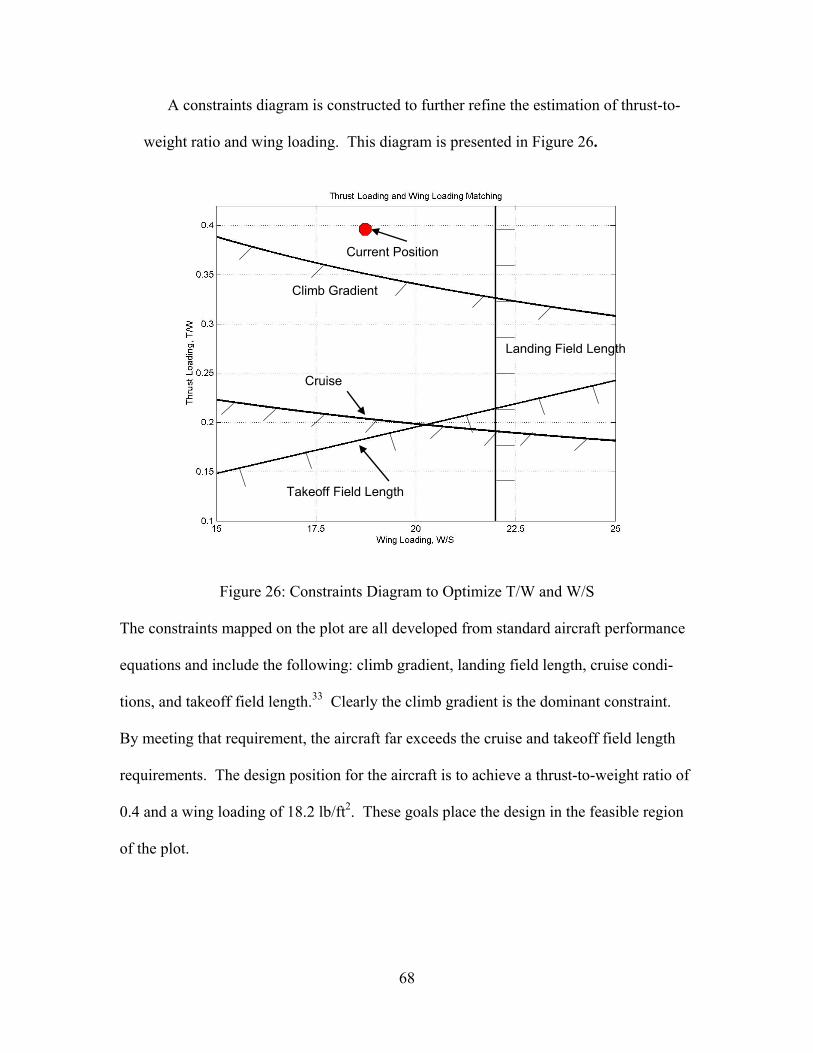
68
A constraints diagram is constructed to further refine the estimation of thrust-to-
weight ratio and wing loading. This diagram is presented in Figure 26.
Cruise
Takeoff Field Length
Current Position
Climb Gradient
Landing Field Length
Figure 26: Constraints Diagram to Optimize T/W and W/S
The constraints mapped on the plot are all developed from standard aircraft performance
equations and include the following: climb gradient, landing field length, cruise condi-
tions, and takeoff field length.33 Clearly the climb gradient is the dominant constraint.
By meeting that requirement, the aircraft far exceeds the cruise and takeoff field length
requirements. The design position for the aircraft is to achieve a thrust-to-weight ratio of
0.4 and a wing loading of 18.2 lb/ft2. These goals place the design in the feasible region
of the plot.
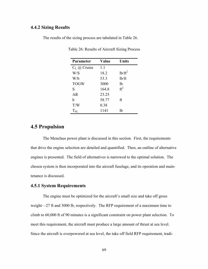
69
4.4.2 Sizing Results
The results of the sizing process are tabulated in Table 26.
Table 26: Results of Aircraft Sizing Process
Parameter Value Units
CL @ Cruise 1.1 W/S 18.2 lb/ft2
W/b 53.3 lb/ft TOGW 3000 lb S 164.8 ft2
AR 23.25 b 58.77 ft T/W 0.38 TSL 1141 lb
4.5 Propulsion
The Menelaus power plant is discussed in this section. First, the requirements
that drive the engine selection are detailed and quantified. Then, an outline of alternative
engines is presented. The field of alternatives is narrowed to the optimal solution. The
chosen system is then incorporated into the aircraft fuselage, and its operation and main-
tenance is discussed.
4.5.1 System Requirements
The engine must be optimized for the aircraft’s small size and take off gross
weight—27 ft and 3000 lb, respectively. The RFP requirement of a maximum time to
climb to 60,000 ft of 90 minutes is a significant constraint on power plant selection. To
meet this requirement, the aircraft must produce a large amount of thrust at sea level.
Since the aircraft is overpowered at sea level, the take off field RFP requirement, tradi-
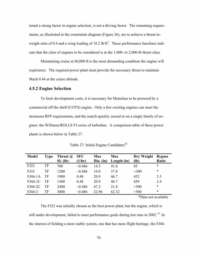
70
tional a strong factor in engine selection, is not a driving factor. The remaining require-
ments, as illustrated in the constraints diagram (Figure 26), are to achieve a thrust-to-
weight ratio of 0.4 and a wing loading of 18.2 lb/ft2. These performance baselines indi-
cate that the class of engines to be considered is in the 1,000- to 2,000-lb thrust class.
Maintaining cruise at 60,000 ft is the most demanding condition the engine will
experience. The required power plant must provide the necessary thrust to maintain
Mach 0.44 at the cruise altitude.
4.5.2 Engine Selection
To limit development costs, it is necessary for Menelaus to be powered by a
commercial off the shelf (COTS) engine. Only a few existing engines can meet the
strenuous RFP requirements, and the search quickly zeroed in on a single family of en-
gines: the Williams/ROLLS FJ series of turbofans. A comparison table of these power
plants is shown below in Table 27.
Table 27: Initial Engine Candidates62
Model Type Thrust @ SL (lb)
SFC (1/hr)
Max Dia. (in)
Max Length (in)
Dry Weight (lb)
Bypass Ratio
FJ22 TF 700 ~0.486 14.5 41.0 85 * FJ33 TF 1200 ~0.486 19.0 37.8 <300 * FJ44-1A TF 1900 0.48 20.9 46.7 452 3.3 FJ44-1C TF 1500 0.48 20.9 46.7 459 3.4 FJ44-2C TF 2400 ~0.486 47.2 21.8 >500 * FJ44-3 TF 3000 ~0.486 22.96 62.32 >500 *
*Data not available
The FJ22 was initially chosen as the best power plant, but the engine, which is
still under development, failed to meet performance goals during test runs in 2002.19 In
the interest of fielding a more stable system, one that has more flight heritage, the FJ44-
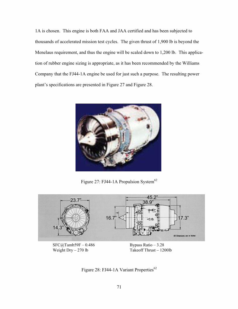
71
1A is chosen. This engine is both FAA and JAA certified and has been subjected to
thousands of accelerated mission test cycles. The given thrust of 1,900 lb is beyond the
Menelaus requirement, and thus the engine will be scaled down to 1,200 lb. This applica-
tion of rubber engine sizing is appropriate, as it has been recommended by the Williams
Company that the FJ44-1A engine be used for just such a purpose. The resulting power
plant’s specifications are presented in Figure 27 and Figure 28.
Figure 27: FJ44-1A Propulsion System62
23.7” 38.9”
17.3”16.7”
14.3”
45.2”
SFC@Tamb59F – 0.486 Bypass Ratio – 3.28Weight Dry – 270 lb Takeoff Thrust – 1200lb
Figure 28: FJ44-1A Variant Properties62

72
4.5.3 FJ44 Performance Characteristics
Williams International provided the engine parameters, with further data being
interpolated via standard on/off performance algorithms. Figure 29 outlines the variation
in thrust as the engine undergoes variation in altitude and Mach number. The engine’s
specific fuel consumption (SFC) under various conditions is also highlighted. Although
the power plant performs adequately in every respect, the values for SFC are larger than
desired. This is due to the adaptation of this system into a flight profile that is higher in
altitude than the engine design conditions. As conformation of the takeoff and landing
performance of the aircraft, Figure 30 shows takeoff thrust rating as affected by various
altitudes and ambient temperatures. This series of data indicates that excess power is
provided under all reasonable field conditions.
Figure 29: Net Thrust and SFC for FJ44 Variant

73
Figure 30: Take-off Thrust under Varying Conditions
4.5.4 Engine Ducting
Two engine placement configurations are practical in the Menelaus airframe. The
first is to enclose the engine and avionics in an attached pod above the fuselage, as in the
Northrop Grumman Global Hawk aircraft. This option is the most simplistic and requires
minimal alteration to the airframe. The second is to integrate the engine into the fuse-
lage, requiring ducting to deliver airflow from the inlet to the power plant. This latter
option is used in the Altair, a new derivative of the General Atomics Predator B. This
configuration allows for the thrust to be produced along the fuselage’s axis of symmetry,
reducing the thrust-induced pitching moment. Additionally, the lack of an external en-
gine pod decreases parasite drag. Due to these benefits, the embedded engine position is
chosen and a standard rectangular to circular ducted configuration is incorporated into the
design.
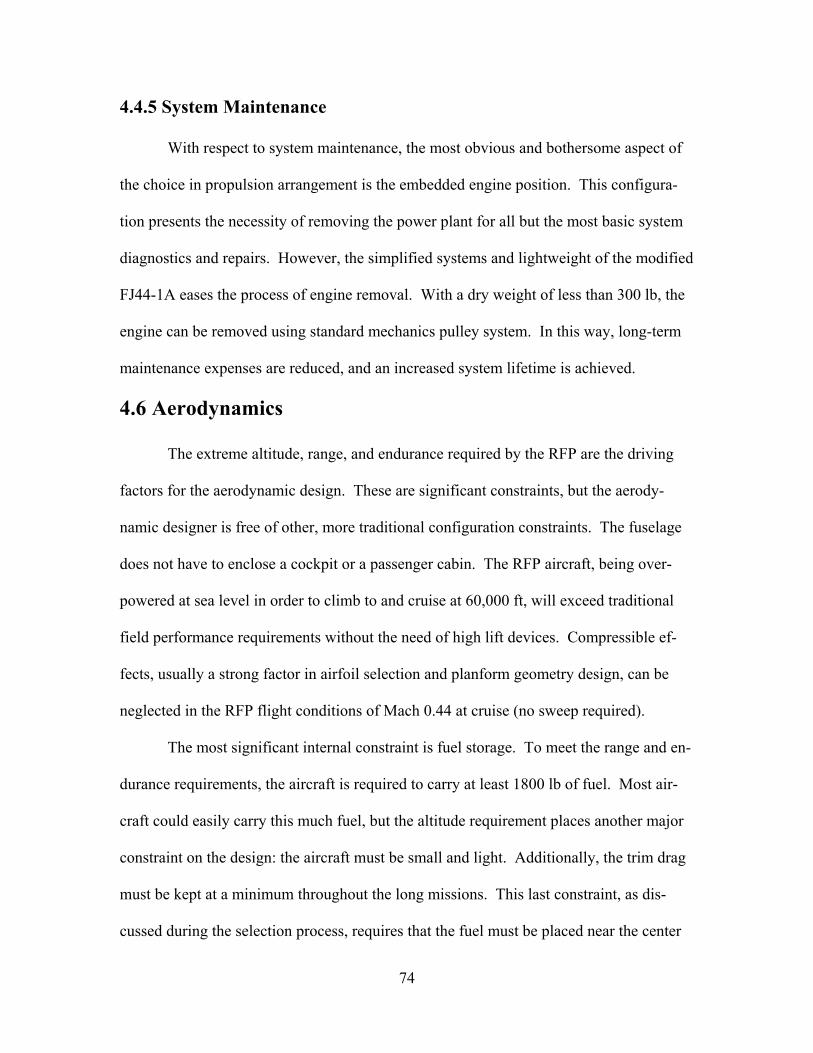
74
4.4.5 System Maintenance
With respect to system maintenance, the most obvious and bothersome aspect of
the choice in propulsion arrangement is the embedded engine position. This configura-
tion presents the necessity of removing the power plant for all but the most basic system
diagnostics and repairs. However, the simplified systems and lightweight of the modified
FJ44-1A eases the process of engine removal. With a dry weight of less than 300 lb, the
engine can be removed using standard mechanics pulley system. In this way, long-term
maintenance expenses are reduced, and an increased system lifetime is achieved.
4.6 Aerodynamics
The extreme altitude, range, and endurance required by the RFP are the driving
factors for the aerodynamic design. These are significant constraints, but the aerody-
namic designer is free of other, more traditional configuration constraints. The fuselage
does not have to enclose a cockpit or a passenger cabin. The RFP aircraft, being over-
powered at sea level in order to climb to and cruise at 60,000 ft, will exceed traditional
field performance requirements without the need of high lift devices. Compressible ef-
fects, usually a strong factor in airfoil selection and planform geometry design, can be
neglected in the RFP flight conditions of Mach 0.44 at cruise (no sweep required).
The most significant internal constraint is fuel storage. To meet the range and en-
durance requirements, the aircraft is required to carry at least 1800 lb of fuel. Most air-
craft could easily carry this much fuel, but the altitude requirement places another major
constraint on the design: the aircraft must be small and light. Additionally, the trim drag
must be kept at a minimum throughout the long missions. This last constraint, as dis-
cussed during the selection process, requires that the fuel must be placed near the center

75
of gravity. The best way to place a large amount of fuel in the shortest possible longitu-
dinal distribution is to use the wings as fuel tanks; thus the fuel constraint translates into a
constraint on the airfoil thickness-to-chord ratio.
Another constraint on the wing thickness is structural weight. This constraint,
like the fuel capacity constraint, requires a thick airfoil—the thicker the wing spars, the
lighter the structure. The analysis, however, shows that the fuel capacity is the dominant
driver of wing thickness, especially considering the lightweight carbon fiber box beam
construction that is discussed in the structures section.
The goals of the aerodynamic design are to reduce the cruise drag to a minimum,
achieve the appropriate lift-to-drag ratio to meet the range and endurance requirements,
and promote an efficient, lightweight airframe. The drag and lift-to-drag ratio goals can
be achieved with an aircraft that minimizes three-dimensional flow, promotes a nearly
elliptical spanwise lift distribution, and minimizes cross sectional and wetted surface
area.
The aerodynamic analysis is presented in this section in the following subsec-
tions: Configuration Design, in which the choices of aircraft geometry are presented and
justified; Airfoil, in which the airfoil choices and dimensioning are discussed; Computa-
tional Aerodynamic Analysis, in which the results of computer simulation iterations are
discussed; and Final Aerodynamic Configuration, in which the final choices for aerody-
namics are compiled and presented.
4.6.1 Configuration Design
The configuration design begins with incorporating the changes discussed at the
end of the concept selection process into the design and justifying the changes with

76
analysis. A shorter, more compact aircraft is qualitatively desirable. It is assumed that
such an aircraft would create less drag and would be lighter and simpler. Also, if the fuel
were contained in the wings, the change in center of gravity position during flight would
be small, eliminating the need for three pitch control surfaces.
To validate shortening the aircraft, a drag analysis of the old and new configura-
tions is performed. The Friction.f program, which calculates the viscous drag, requires
the basic dimensions of the aircraft and the flight conditions.51 For simplicity, the air-
craft’s fuselage and booms are modeled as cylinders and the wings are modeled as plates
with finite thickness. The flight conditions are taken from the cruise requirements of the
RFP (60,000 ft, 250 ktas). The Reynolds number for this aircraft at cruise is 840,000,
which is above the limit for flat plate transition from laminar to turbulent flow (500,000).
This limit, however, can be exceeded by carefully choosing aerodynamic surface shapes
that sustain favorable pressure gradients as long as possible. With this in mind, laminar
flow is assumed in the Friction.f calculations.
The analysis shows that the changes in configuration afforded an 11% reduction
in wetted surface area and a reduction in drag coefficient of 8%. The drag coefficient
discussed here is the combination of friction drag and form drag, but does not include the
induced drag, which is calculated in a later section. These results justify the shortening
of the aircraft and are presented in Table 28.
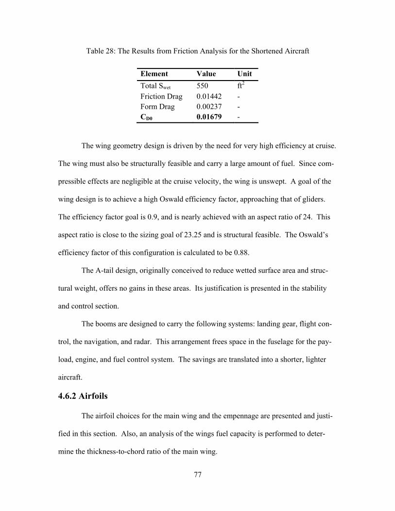
77
Table 28: The Results from Friction Analysis for the Shortened Aircraft
Element Value Unit
Total Swet 550 ft2
Friction Drag 0.01442 - Form Drag 0.00237 - CD0 0.01679 -
The wing geometry design is driven by the need for very high efficiency at cruise.
The wing must also be structurally feasible and carry a large amount of fuel. Since com-
pressible effects are negligible at the cruise velocity, the wing is unswept. A goal of the
wing design is to achieve a high Oswald efficiency factor, approaching that of gliders.
The efficiency factor goal is 0.9, and is nearly achieved with an aspect ratio of 24. This
aspect ratio is close to the sizing goal of 23.25 and is structural feasible. The Oswald’s
efficiency factor of this configuration is calculated to be 0.88.
The A-tail design, originally conceived to reduce wetted surface area and struc-
tural weight, offers no gains in these areas. Its justification is presented in the stability
and control section.
The booms are designed to carry the following systems: landing gear, flight con-
trol, the navigation, and radar. This arrangement frees space in the fuselage for the pay-
load, engine, and fuel control system. The savings are translated into a shorter, lighter
aircraft.
4.6.2 Airfoils
The airfoil choices for the main wing and the empennage are presented and justi-
fied in this section. Also, an analysis of the wings fuel capacity is performed to deter-
mine the thickness-to-chord ratio of the main wing.

78
Figure 31: The Main Wing Airfoil - NASA/Langley/Whitcomb LS(1)-0417 (GA(W))57
The main wing airfoil choice is the NASA/Langley/Whitcomb LS(1)-0417
(GA(W)) airfoil (Figure 31). This class of airfoils shows excellent low speed characteris-
tics and has good stall performance. The maximum thickness, and therefore the position
of the minimum pressures, is relatively far aft at 40% of the chord, and the change in
thickness is small through the central part of the airfoil. This arrangement delays the on-
set of an adverse pressure gradient and produces a gradual change in pressure over most
of the airfoil. The lift distribution shows an even spread along the length of the chord,
with no sharp peaks near the leading edge. These aerodynamic properties promote lami-
nar flow and thus low drag. The thickness of the central section of the airfoil is also de-
sirable for fuel capacity and structural design. This family of airfoils is used on Predator
B, a successful high altitude UAV design.
The airfoil choice for the tail surfaces is a NACA 64-012 symmetric, laminar flow
airfoil. The thickness-to-chord ratio is chosen to be 0.12, which is a good compromise
between low drag and structural design. The airfoil section for the empennage is shown
in Figure 32.
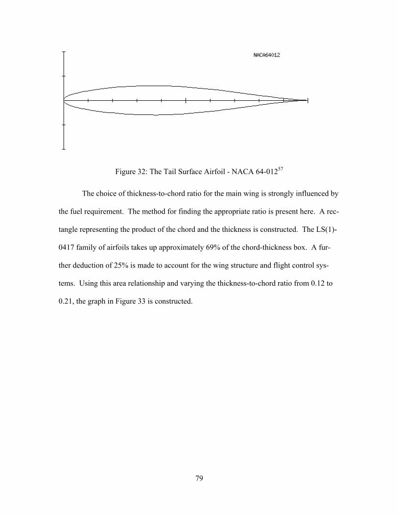
79
Figure 32: The Tail Surface Airfoil - NACA 64-01257
The choice of thickness-to-chord ratio for the main wing is strongly influenced by
the fuel requirement. The method for finding the appropriate ratio is present here. A rec-
tangle representing the product of the chord and the thickness is constructed. The LS(1)-
0417 family of airfoils takes up approximately 69% of the chord-thickness box. A fur-
ther deduction of 25% is made to account for the wing structure and flight control sys-
tems. Using this area relationship and varying the thickness-to-chord ratio from 0.12 to
0.21, the graph in Figure 33 is constructed.

80
Figure 33: Main Wing Thickness-to-Chord Ratio and Wing Fuel Capacity
The target weight for fuel is 1800 lb, 1600 lb of which should be carried in the wings.
This target value, shown in the graph as a vertical line, leads to a thickness-to-chord ratio
of 17.2%. The ratio is set at 17%, leaving additional required fuel to be stored in the fu-
selage tank.
With the airfoils chosen, and the thickness-to-chord ratio set, a more detailed
analysis of the flow over the airfoil is made. First the inviscid solution of the flow over
the LS(1)-0417 airfoil is found using a vortex lattice method code.20 The resultant veloc-
ity profile is then plugged into a code that calculates incompressible, laminar boundary
layers with Waltz’s integral method. This method, not accurate enough for detailed air-
foil analysis, will provide enough information to test the assumption of laminar flow

81
made in earlier analysis. The calculation will show if the flow experiences transition, and
approximately where that transition occurs. The input information is presented in Table
29.
Table 29: Input Data for Boundary Layer Analysis
Fluid Properties Viscosity (m^2/s) = 1.222e-4 Reference Properties Freestream velocity (m/s) = 128.6 Reference length L (m) = 0.805 Surface Characteristics 2D body, rounded leading edge = 1 Pressure profile determined by velocity profile Calculation Parameters Maximum x/L = 1 Number of x steps = 201
Figure 34 shows the results from the boundary layer calculation. The upper plot
shows the velocity profile (which is directly related to the pressure profile) and the bot-
tom plot shows the boundary layer growth and location of the beginning of the transition.
The results indicate that the flow experiences transition at nearly 60% of the chord aft of
the leading edge. This transition is far enough aft to support the assumptions of laminar
flow in the Fiction.f calculations, but could be improved upon. Designing custom airfoils
for specific aircraft has become an increasingly affordable option (X-Foil is a free airfoil
design software package). These airfoils typically exceed the performance of “off the
shelf” airfoils, like the LS(1)-0417 (GA(W)).

82
Figure 34: Results from Boundary Layer Analysis
4.6.3 Computational Aerodynamic Analysis
The main tool used to analyze the aerodynamics of the design is Tornado, a
MATLAB vortex lattice method code.54 The configuration is run through multiple itera-
tions, systematically altering the wing area, aspect ratio, span, main wing incidence angle
and location, tail boom length, tail surface area, and angle of attack. These iterations and
other analysis performed in the stability and control section lead to the final configura-
tion, which is presented at the end of this section.
The Tornado program, like other vortex lattice programs, assumes irrotational and
inviscid flow, but it differs form other codes in its treatment of the trailing vortices. In-
stead of idealizing the trailing vortex system as a three-piece horseshoe, Tornado divides
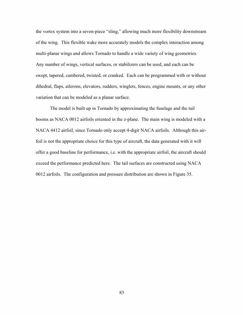
83
the vortex system into a seven-piece “sling,” allowing much more flexibility downstream
of the wing. This flexible wake more accurately models the complex interaction among
multi-planar wings and allows Tornado to handle a wide variety of wing geometries.
Any number of wings, vertical surfaces, or stabilizers can be used, and each can be
swept, tapered, cambered, twisted, or cranked. Each can be programmed with or without
dihedral, flaps, ailerons, elevators, rudders, winglets, fences, engine mounts, or any other
variation that can be modeled as a planar surface.
The model is built up in Tornado by approximating the fuselage and the tail
booms as NACA 0012 airfoils oriented in the z-plane. The main wing is modeled with a
NACA 4412 airfoil, since Tornado only accept 4-digit NACA airfoils. Although this air-
foil is not the appropriate choice for this type of aircraft, the data generated with it will
offer a good baseline for performance, i.e. with the appropriate airfoil, the aircraft should
exceed the performance predicted here. The tail surfaces are constructed using NACA
0012 airfoils. The configuration and pressure distribution are shown in Figure 35.
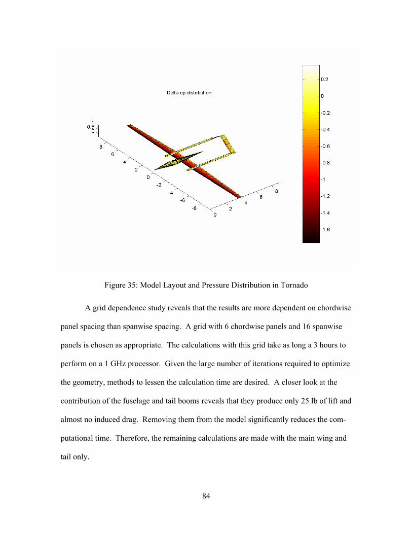
84
Figure 35: Model Layout and Pressure Distribution in Tornado
A grid dependence study reveals that the results are more dependent on chordwise
panel spacing than spanwise spacing. A grid with 6 chordwise panels and 16 spanwise
panels is chosen as appropriate. The calculations with this grid take as long a 3 hours to
perform on a 1 GHz processor. Given the large number of iterations required to optimize
the geometry, methods to lessen the calculation time are desired. A closer look at the
contribution of the fuselage and tail booms reveals that they produce only 25 lb of lift and
almost no induced drag. Removing them from the model significantly reduces the com-
putational time. Therefore, the remaining calculations are made with the main wing and
tail only.
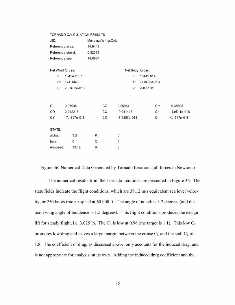
85
TORNADO CALCULATION RESULTS
JID: MenelausWingsOnly
Reference area: 14.9443
Reference chord: 0.82379
Reference span: 18.8967
Net Wind forces:
L: 13454.2387
D: 171.1446
S: -1.0492e-013
Net Body forces:
Z: 13442.814
X: -1.0492e-013
Y: -580.1581
CL 0.96046
CD 0.012218
CY -7.4897e-018
CZ 0.95964
CX -0.041416
CC -7.4897e-018
Cm -0.38505
Cn -1.9511e-018
Cl 4.1547e-018
STATE:
alpha: 3.2
beta: 0
Airspeed: 39.12
P: 0
Q: 0
R: 0
Figure 36: Numerical Data Generated by Tornado Iterations (all forces in Newtons)
The numerical results from the Tornado iterations are presented in Figure 36. The
state fields indicate the flight conditions, which are 39.12 m/s equivalent sea level veloc-
ity, or 250 knots true air speed at 60,000 ft. The angle of attack is 3.2 degrees (and the
main wing angle of incidence is 1.5 degrees). This flight conditions produces the design
lift for steady flight, i.e. 3,025 lb. The CL is low at 0.96 (the target is 1.1). This low CL
promotes low drag and leaves a large margin between the cruise CL and the stall CL of
1.8. The coefficient of drag, as discussed above, only accounts for the induced drag, and
is not appropriate for analysis on its own. Adding the induced drag coefficient and the
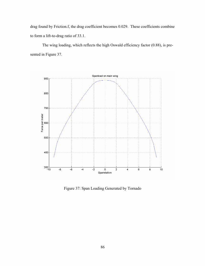
86
drag found by Friction.f, the drag coefficient becomes 0.029. These coefficients combine
to form a lift-to-drag ratio of 33.1.
The wing loading, which reflects the high Oswald efficiency factor (0.88), is pre-
sented in Figure 37.
Figure 37: Span Loading Generated by Tornado
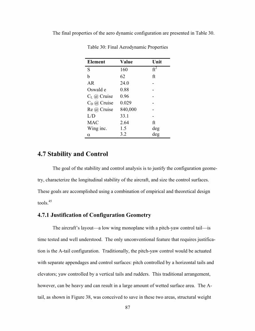
87
The final properties of the aero dynamic configuration are presented in Table 30.
Table 30: Final Aerodynamic Properties
Element Value Unit
S 160 ft2
b 62 ft AR 24.0 - Oswald e 0.88 - CL @ Cruise 0.96 - CD @ Cruise 0.029 - Re @ Cruise 840,000 - L/D 33.1 - MAC 2.64 ft Wing inc. 1.5 deg α 3.2 deg
4.7 Stability and Control
The goal of the stability and control analysis is to justify the configuration geome-
try, characterize the longitudinal stability of the aircraft, and size the control surfaces.
These goals are accomplished using a combination of empirical and theoretical design
tools.45
4.7.1 Justification of Configuration Geometry
The aircraft’s layout—a low wing monoplane with a pitch-yaw control tail—is
time tested and well understood. The only unconventional feature that requires justifica-
tion is the A-tail configuration. Traditionally, the pitch-yaw control would be actuated
with separate appendages and control surfaces: pitch controlled by a horizontal tails and
elevators; yaw controlled by a vertical tails and rudders. This traditional arrangement,
however, can be heavy and can result in a large amount of wetted surface area. The A-
tail, as shown in Figure 38, was conceived to save in these two areas, structural weight
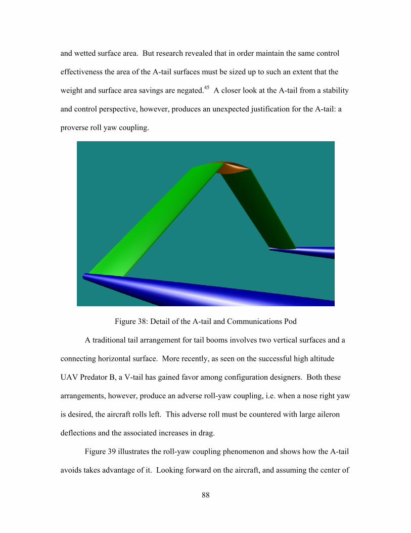
88
and wetted surface area. But research revealed that in order maintain the same control
effectiveness the area of the A-tail surfaces must be sized up to such an extent that the
weight and surface area savings are negated.45 A closer look at the A-tail from a stability
and control perspective, however, produces an unexpected justification for the A-tail: a
proverse roll yaw coupling.
Figure 38: Detail of the A-tail and Communications Pod
A traditional tail arrangement for tail booms involves two vertical surfaces and a
connecting horizontal surface. More recently, as seen on the successful high altitude
UAV Predator B, a V-tail has gained favor among configuration designers. Both these
arrangements, however, produce an adverse roll-yaw coupling, i.e. when a nose right yaw
is desired, the aircraft rolls left. This adverse roll must be countered with large aileron
deflections and the associated increases in drag.
Figure 39 illustrates the roll-yaw coupling phenomenon and shows how the A-tail
avoids takes advantage of it. Looking forward on the aircraft, and assuming the center of

89
gravity is located at the center of the fuselage, it is easy to see that the forces required to
produce a nose right yaw will produce a right roll in both the V-tail and the traditional
tail. The same maneuver actuated by the A-tail produces a favorable roll-yaw coupling,
and reduced drag during the maneuver. In addition to this control advantage (which
alone could justify the configuration), the A-tail works well with the engine and boom
layout and affords convenient placement of the satellite communication dome.
(a) V-Tail
(b) Traditional Tail
(c) A-Tail
Figure 39: Illustration of Roll-Yaw Coupling
4.7.2 Static Margin
The static margin of typical commercial transport aircraft is between 5% and 10%
stable. This level of longitudinal stability produces aircraft that pilots can handle easily
and that can fly efficiently in many different loading conditions. But the gains in han-
dling qualities and center of gravity range come at the price of trim drag at cruise and re-
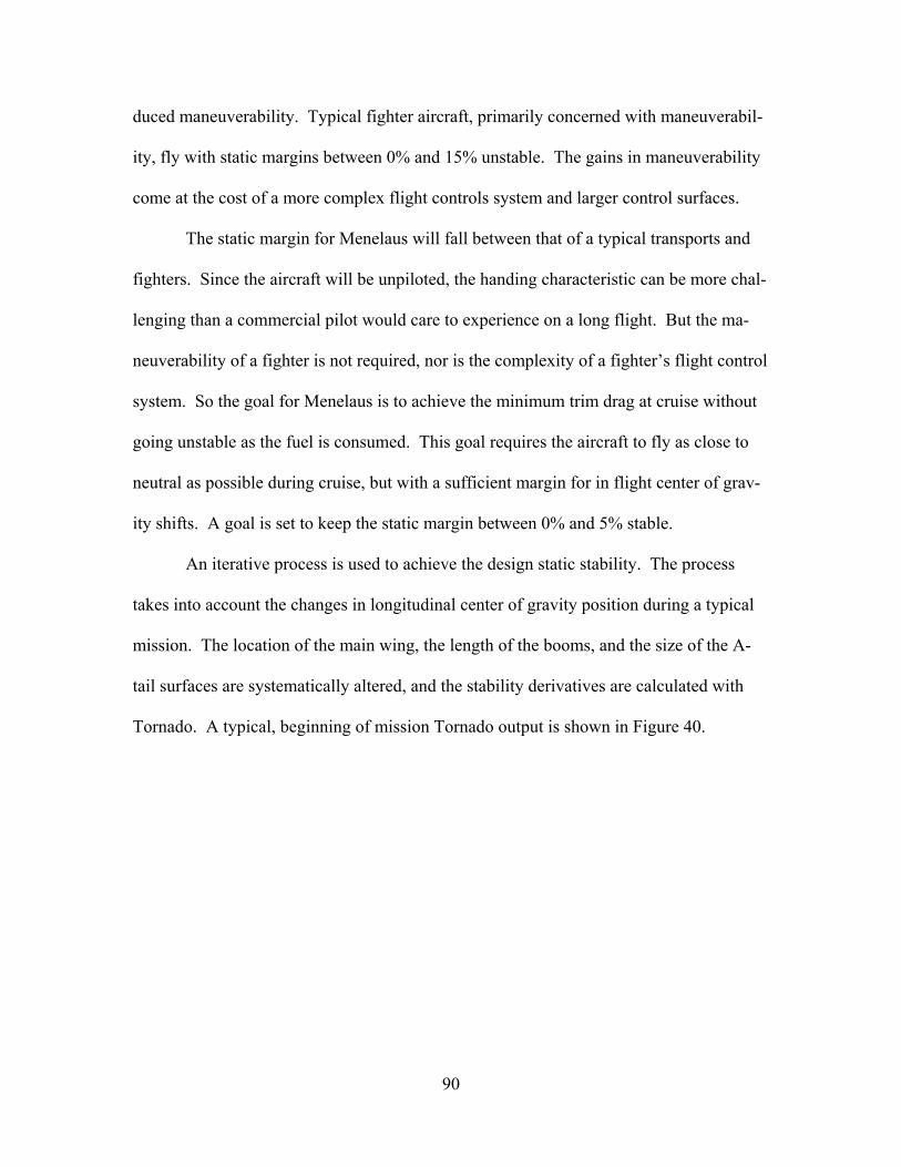
90
duced maneuverability. Typical fighter aircraft, primarily concerned with maneuverabil-
ity, fly with static margins between 0% and 15% unstable. The gains in maneuverability
come at the cost of a more complex flight controls system and larger control surfaces.
The static margin for Menelaus will fall between that of a typical transports and
fighters. Since the aircraft will be unpiloted, the handing characteristic can be more chal-
lenging than a commercial pilot would care to experience on a long flight. But the ma-
neuverability of a fighter is not required, nor is the complexity of a fighter’s flight control
system. So the goal for Menelaus is to achieve the minimum trim drag at cruise without
going unstable as the fuel is consumed. This goal requires the aircraft to fly as close to
neutral as possible during cruise, but with a sufficient margin for in flight center of grav-
ity shifts. A goal is set to keep the static margin between 0% and 5% stable.
An iterative process is used to achieve the design static stability. The process
takes into account the changes in longitudinal center of gravity position during a typical
mission. The location of the main wing, the length of the booms, and the size of the A-
tail surfaces are systematically altered, and the stability derivatives are calculated with
Tornado. A typical, beginning of mission Tornado output is shown in Figure 40.
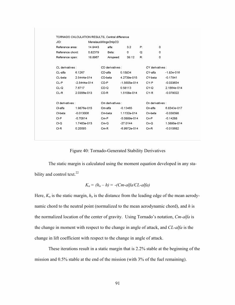
91
Figure 40: Tornado-Generated Stability Derivatives
The static margin is calculated using the moment equation developed in any sta-
bility and control text.22
Kn = (hn – h) = -(Cm-alfa/CL-alfa)
Here, Kn is the static margin, hn is the distance from the leading edge of the mean aerody-
namic chord to the neutral point (normalized to the mean aerodynamic chord), and h is
the normalized location of the center of gravity. Using Tornado’s notation, Cm-alfa is
the change in moment with respect to the change in angle of attack, and CL-alfa is the
change in lift coefficient with respect to the change in angle of attack.
These iterations result in a static margin that is 2.2% stable at the beginning of the
mission and 0.5% stable at the end of the mission (with 3% of the fuel remaining).
92
4.7.3 Control Surface Sizing
Typical aircraft design sizing algorithms for control surfaces generally result in
control surfaces that were too large for Menelaus. Therefore, existing high altitude, long
endurance/range aircraft are used as a guide for surface sizing, and Tornado is used to
validate the choices.
For aileron sizing, a rule of thumb approach leads to surfaces that are 20% to 25%
of the wings chord, and extend from 50% to 90% of the wing’s semispan.45 Ailerons of
this size, place so far outboard, would most likely result in control reversal for such a
high aspect ratio wing, and are unnecessary for the types of maneuvers Menelaus is ex-
pected to perform.
Figure 41: Perseus B Aileron Size and Location39
Perseus B, designed be Aurora Flight Sciences, is a high altitude UAV that
closely matches the size of Menelaus. The photograph in Figure 41 shows the size and

93
location one of the ailerons. The surface is about 15% of the chord in the chordwise di-
rection and 20% of the semispan in the spanwise direction. It is located between 40%
and 60% of the semispan outboard. Tornado analysis, however, shows that these surfaces
are too small for Menelaus. Sizing them up to 20% of the chord and 28% of the semis-
pan and locating them between 39% and 67% of the semispan outboard lead to reason-
able results from Tornado. The resultant ailerons are 4.2 ft2 each and are shown in Figure
42.
Figure 42: Menelaus Aileron Size and Location (all dimensions in ft)
The V-tail ruddervators on Predator B, a General Atomics high altitude UAV, are
used as a model for the A-tail surface sizing. Although the V-tail and A-tail look differ-
ent and produce different roll-yaw coupling, they are required to generate essentially the
same forces for controlling the aircraft. The size of the control surfaces should be the
same. Predator’s control surfaces are shown in Figure 43. They are about 20% of the
chord in the chordwise direction and extend the entire length of the tail surface in the
spanwise direction. To make up for the extra control force Predator generates with the
ventral vertical surface, the ruddervators for Menelaus are sized up to 25% the chord in
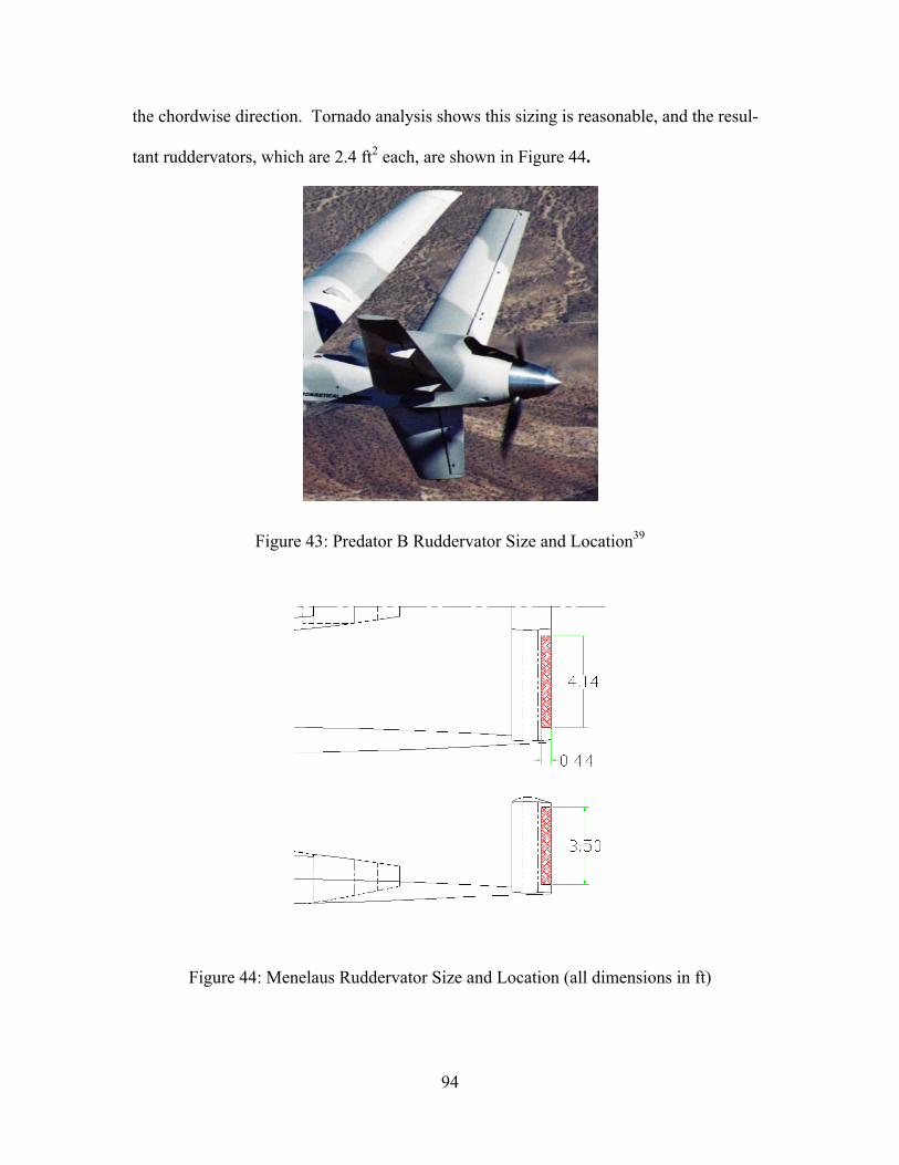
94
the chordwise direction. Tornado analysis shows this sizing is reasonable, and the resul-
tant ruddervators, which are 2.4 ft2 each, are shown in Figure 44.
Figure 43: Predator B Ruddervator Size and Location39
Figure 44: Menelaus Ruddervator Size and Location (all dimensions in ft)
95
4.8 Performance
Many aircraft exist that some or most of the RFP requirements. The central justi-
fication of this design project is to improve upon previous designs and to generate a vi-
able platform that meets all of the RFP requirements. The quantitative measures of mis-
sion success are the Menelaus performance characteristics. In this section, the aircraft
design’s performance is calculated and compared to the RFP requirements.
4.8.1 Mission Profile Analysis
The Virginia Tech Mission Program is used to calculate the design aircraft’s per-
formance. The measures of effectiveness are taken from the RFP and are listed as fol-
lows: cruise altitude (60,000 ft), range (7,000 NM), endurance (36 hours), and time to
climb (90 minutes).
The following two missions were modeled in the mission analysis program:
1 – Twenty Minute Loiter Time at Full Thrust (simulating taxi, etc…)
2 – Climb to 60,000 ft. Using Best Rate of Climb
3 – Cruise at 60,000 ft. at Mach 0.44 for over 8,000 NM
4 – Descend to Sea Level
1 – Twenty Minute Loiter Time at Full Thrust (simulating taxi, etc…)
2 – Climb to 60,000 ft. Using Best Rate of Climb
3 – Cruise at 60,000 ft. at Mach 0.38 for over 7,000 NM
4 – Descend to Sea Level
Analysis of the two outputs serves to validate the ability of Menelaus to meet all
of the RFP requirements. In both cases, more than a 300 lb of fuel remains at the end of
the mission; therefore the missions are plausible. In the first mission a sea level climb
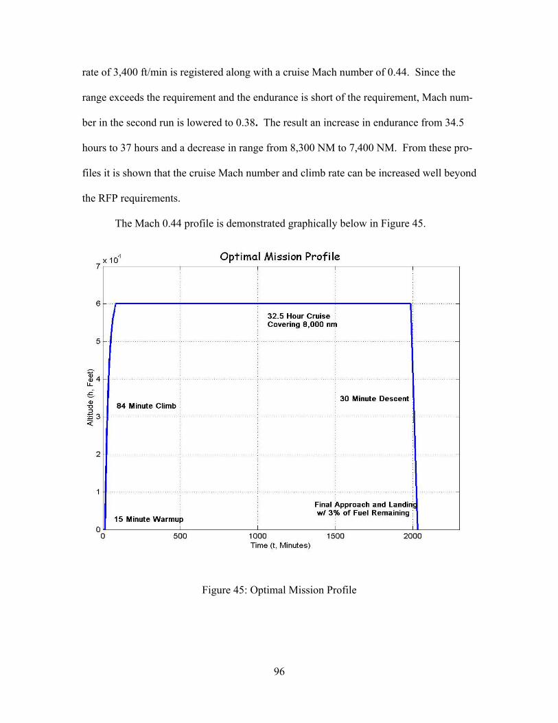
96
rate of 3,400 ft/min is registered along with a cruise Mach number of 0.44. Since the
range exceeds the requirement and the endurance is short of the requirement, Mach num-
ber in the second run is lowered to 0.38. The result an increase in endurance from 34.5
hours to 37 hours and a decrease in range from 8,300 NM to 7,400 NM. From these pro-
files it is shown that the cruise Mach number and climb rate can be increased well beyond
the RFP requirements.
The Mach 0.44 profile is demonstrated graphically below in Figure 45.
Figure 45: Optimal Mission Profile

97
4.8.2 Aircraft Comparison
Justification for the Menelaus program is seen in a comparison between the
aforementioned aircraft and those comparable systems, as seen in Table 31.
Table 31: Menelaus Comparison
98
4.9 Materials and Structure
4.9.1 Materials
Since the Menelaus is a proof of concept aircraft, the main driving factors for the
structural design are as follows:
1) Weight
2) Strength
3) Cost
Table 32 shows the comparison of approximate material cost when the Menelaus is con-
structed with different materials for each major component. The heaviest configuration is
the one in which all major components are constructed with Aluminum. The lightest
configuration is the one in which the wings, A-tail, fuselage, and booms are constructed
with carbon fiber and landing gear, engine mount, and payload interface is constructed
with Aluminum. Carbon fiber is approximate 50% lighter and 500% more expensive
than Aluminum. Carbon fiber also comes with higher tensile and yield strength per unit
weight than Aluminum. Although the mostly carbon fiber aircraft is easily the most ex-
pensive, mission analysis has shown that it is the only configuration that can meet the
RFP requirements.
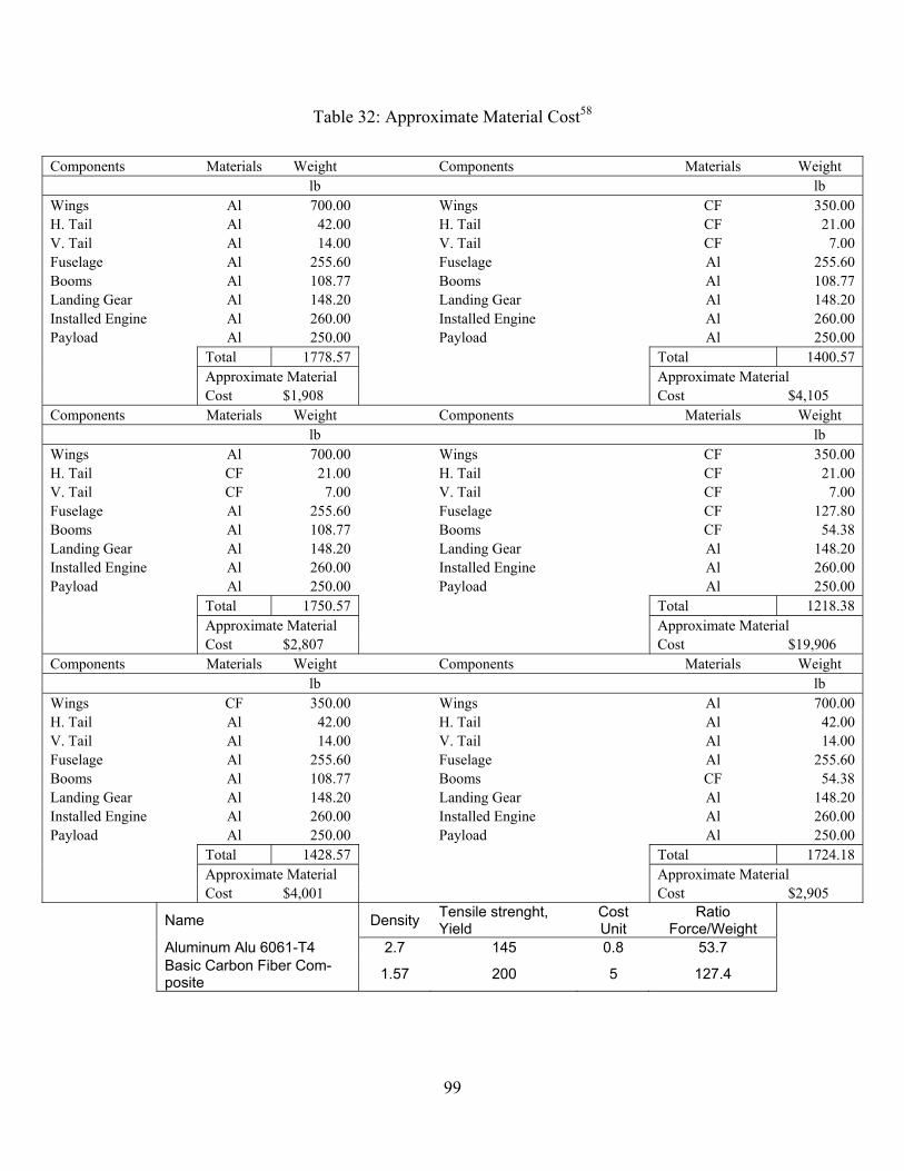
99
Table 32: Approximate Material Cost58
Components Materials Weight Components Materials Weight lb lb Wings Al 700.00 Wings CF 350.00 H. Tail Al 42.00 H. Tail CF 21.00 V. Tail Al 14.00 V. Tail CF 7.00 Fuselage Al 255.60 Fuselage Al 255.60 Booms Al 108.77 Booms Al 108.77 Landing Gear Al 148.20 Landing Gear Al 148.20 Installed Engine Al 260.00 Installed Engine Al 260.00 Payload Al 250.00 Payload Al 250.00 Total 1778.57 Total 1400.57 Approximate Material Approximate Material Cost $1,908 Cost $4,105 Components Materials Weight Components Materials Weight lb lb Wings Al 700.00 Wings CF 350.00 H. Tail CF 21.00 H. Tail CF 21.00 V. Tail CF 7.00 V. Tail CF 7.00 Fuselage Al 255.60 Fuselage CF 127.80 Booms Al 108.77 Booms CF 54.38 Landing Gear Al 148.20 Landing Gear Al 148.20 Installed Engine Al 260.00 Installed Engine Al 260.00 Payload Al 250.00 Payload Al 250.00 Total 1750.57 Total 1218.38 Approximate Material Approximate Material Cost $2,807 Cost $19,906 Components Materials Weight Components Materials Weight lb lb Wings CF 350.00 Wings Al 700.00 H. Tail Al 42.00 H. Tail Al 42.00 V. Tail Al 14.00 V. Tail Al 14.00 Fuselage Al 255.60 Fuselage Al 255.60 Booms Al 108.77 Booms CF 54.38 Landing Gear Al 148.20 Landing Gear Al 148.20 Installed Engine Al 260.00 Installed Engine Al 260.00 Payload Al 250.00 Payload Al 250.00 Total 1428.57 Total 1724.18 Approximate Material Approximate Material Cost $4,001 Cost $2,905
Name Density Tensile strenght, Yield
Cost Unit
Ratio Force/Weight
Aluminum Alu 6061-T4 2.7 145 0.8 53.7
Basic Carbon Fiber Com-posite 1.57 200 5 127.4
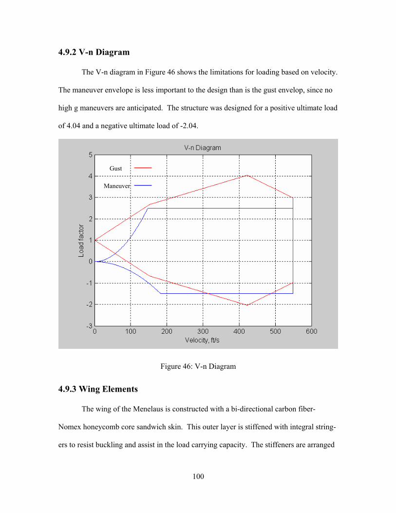
100
4.9.2 V-n Diagram
The V-n diagram in Figure 46 shows the limitations for loading based on velocity.
The maneuver envelope is less important to the design than is the gust envelop, since no
high g maneuvers are anticipated. The structure was designed for a positive ultimate load
of 4.04 and a negative ultimate load of -2.04.
Figure 46: V-n Diagram
4.9.3 Wing Elements
The wing of the Menelaus is constructed with a bi-directional carbon fiber-
Nomex honeycomb core sandwich skin. This outer layer is stiffened with integral string-
ers to resist buckling and assist in the load carrying capacity. The stiffeners are arranged
Gust
Maneuver
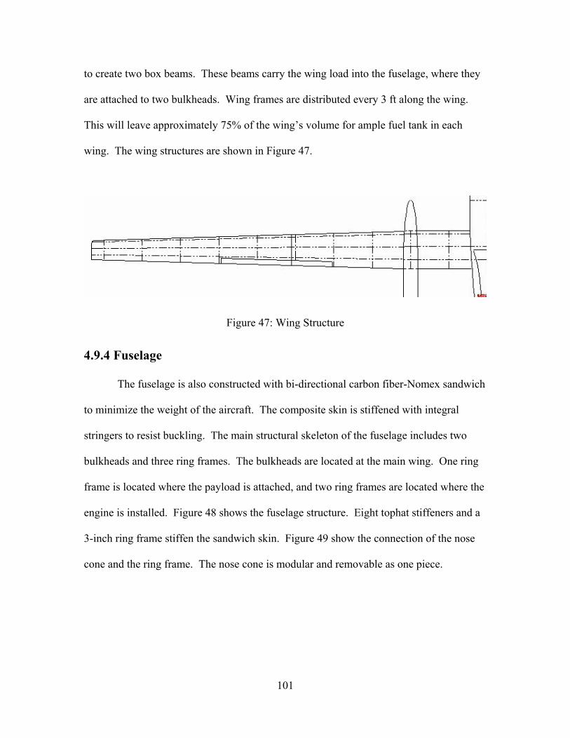
101
to create two box beams. These beams carry the wing load into the fuselage, where they
are attached to two bulkheads. Wing frames are distributed every 3 ft along the wing.
This will leave approximately 75% of the wing’s volume for ample fuel tank in each
wing. The wing structures are shown in Figure 47.
Figure 47: Wing Structure
4.9.4 Fuselage
The fuselage is also constructed with bi-directional carbon fiber-Nomex sandwich
to minimize the weight of the aircraft. The composite skin is stiffened with integral
stringers to resist buckling. The main structural skeleton of the fuselage includes two
bulkheads and three ring frames. The bulkheads are located at the main wing. One ring
frame is located where the payload is attached, and two ring frames are located where the
engine is installed. Figure 48 shows the fuselage structure. Eight tophat stiffeners and a
3-inch ring frame stiffen the sandwich skin. Figure 49 show the connection of the nose
cone and the ring frame. The nose cone is modular and removable as one piece.
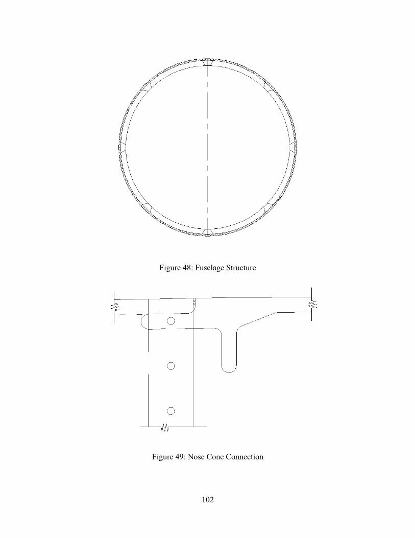
102
Figure 48: Fuselage Structure
Figure 49: Nose Cone Connection
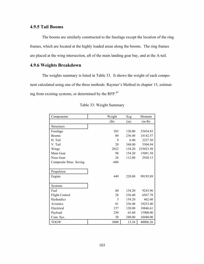
103
4.9.5 Tail Booms
The booms are similarly constructed to the fuselage except the location of the ring
frames, which are located at the highly loaded areas along the booms. The ring frames
are placed at the wing intersection, aft of the main landing gear bay, and at the A-tail.
4.9.6 Weights Breakdown
The weights summary is listed in Table 33. It shows the weight of each compo-
nent calculated using one of the three methods: Raymer’s Method in chapter 15, estimat-
ing from existing systems, or determined by the RFP.45
Table 33: Weight Summary
Components Weight Xcg Moment (lb) (in) (in-lb) Structures Fuselage 283 120.00 25454.83 Booms 80 236.40 14142.57 H. Tail 9 6.40 2227.30 V. Tail 20 348.00 5304.94 Wings 2032 154.20 235023.50 Main Gear 98 154.20 15091.58 Nose Gear 26 112.80 2920.13 Composite Struc. Saving -606 Propulsion Engine 449 220.80 99195.89 Systems Fuel 60 154.20 9243.96 Flight Control 28 236.40 6567.78 Hydraulics 3 154.20 462.60 Avionics 81 236.40 19253.40 Electrical 157 120.00 18846.61 Payload 250 63.60 15900.00 Com. Sys. 30 348.00 10440.00 TOGW 3000 13.34 40006.26
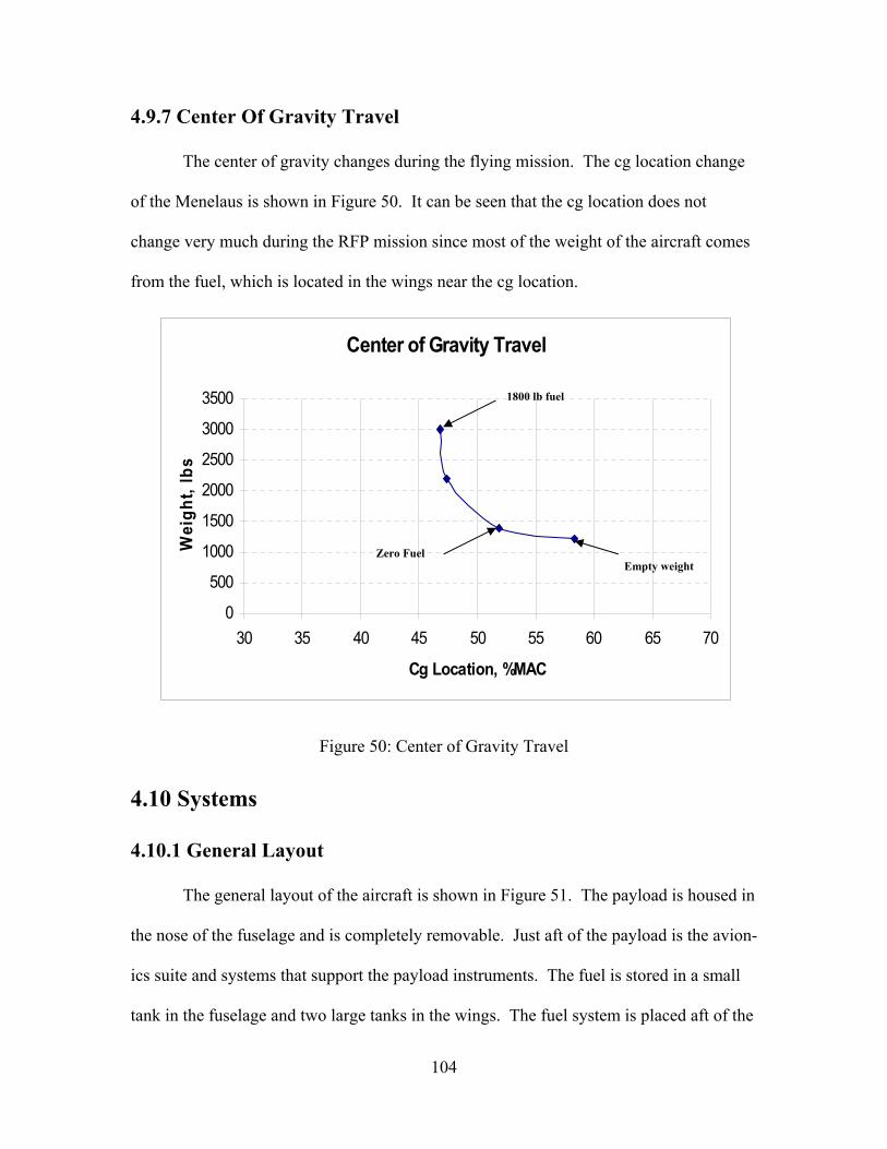
104
4.9.7 Center Of Gravity Travel
The center of gravity changes during the flying mission. The cg location change
of the Menelaus is shown in Figure 50. It can be seen that the cg location does not
change very much during the RFP mission since most of the weight of the aircraft comes
from the fuel, which is located in the wings near the cg location.
Center of Gravity Travel
0
500
1000
1500
2000
2500
3000
3500
30 35 40 45 50 55 60 65 70
Cg Location, %MAC
Wei
ght,
lbs
Figure 50: Center of Gravity Travel
4.10 Systems
4.10.1 General Layout
The general layout of the aircraft is shown in Figure 51. The payload is housed in
the nose of the fuselage and is completely removable. Just aft of the payload is the avion-
ics suite and systems that support the payload instruments. The fuel is stored in a small
tank in the fuselage and two large tanks in the wings. The fuel system is placed aft of the
1800 lb fuel
Zero Fuel Empty weight
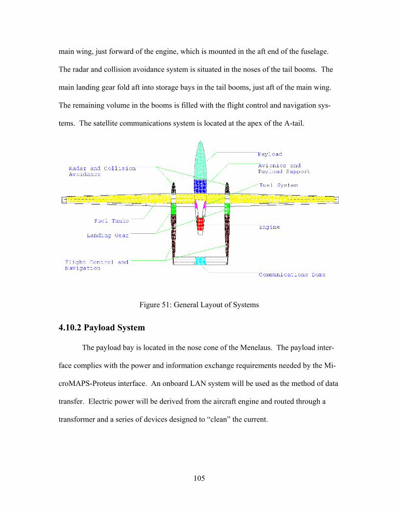
105
main wing, just forward of the engine, which is mounted in the aft end of the fuselage.
The radar and collision avoidance system is situated in the noses of the tail booms. The
main landing gear fold aft into storage bays in the tail booms, just aft of the main wing.
The remaining volume in the booms is filled with the flight control and navigation sys-
tems. The satellite communications system is located at the apex of the A-tail.
Figure 51: General Layout of Systems
4.10.2 Payload System
The payload bay is located in the nose cone of the Menelaus. The payload inter-
face complies with the power and information exchange requirements needed by the Mi-
croMAPS-Proteus interface. An onboard LAN system will be used as the method of data
transfer. Electric power will be derived from the aircraft engine and routed through a
transformer and a series of devices designed to “clean” the current.
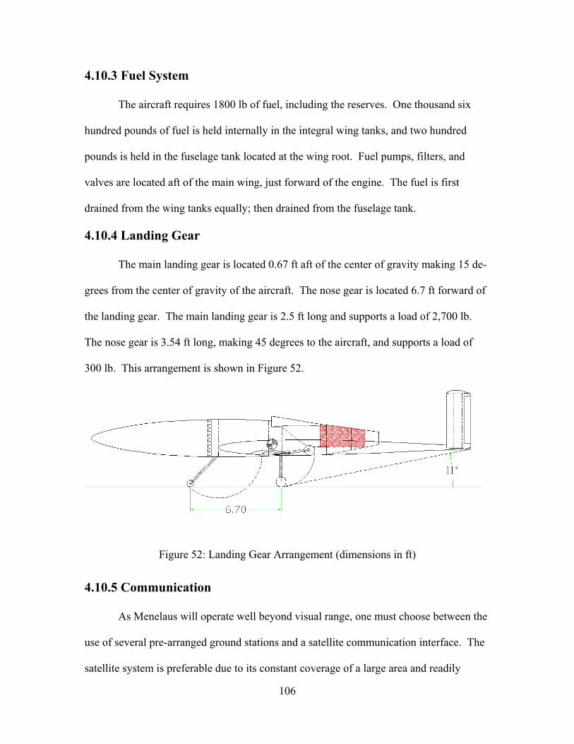
106
4.10.3 Fuel System
The aircraft requires 1800 lb of fuel, including the reserves. One thousand six
hundred pounds of fuel is held internally in the integral wing tanks, and two hundred
pounds is held in the fuselage tank located at the wing root. Fuel pumps, filters, and
valves are located aft of the main wing, just forward of the engine. The fuel is first
drained from the wing tanks equally; then drained from the fuselage tank.
4.10.4 Landing Gear
The main landing gear is located 0.67 ft aft of the center of gravity making 15 de-
grees from the center of gravity of the aircraft. The nose gear is located 6.7 ft forward of
the landing gear. The main landing gear is 2.5 ft long and supports a load of 2,700 lb.
The nose gear is 3.54 ft long, making 45 degrees to the aircraft, and supports a load of
300 lb. This arrangement is shown in Figure 52.
Figure 52: Landing Gear Arrangement (dimensions in ft)
4.10.5 Communication
As Menelaus will operate well beyond visual range, one must choose between the
use of several pre-arranged ground stations and a satellite communication interface. The
satellite system is preferable due to its constant coverage of a large area and readily
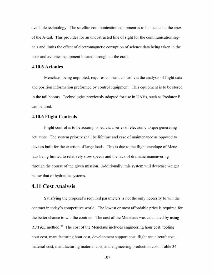
107
available technology. The satellite communication equipment is to be located at the apex
of the A-tail. This provides for an unobstructed line of sight for the communication sig-
nals and limits the effect of electromagnetic corruption of science data being taken in the
nose and avionics equipment located throughout the craft.
4.10.6 Avionics
Menelaus, being unpiloted, requires constant control via the analysis of flight data
and position information preformed by control equipment. This equipment is to be stored
in the tail booms. Technologies previously adapted for use in UAVs, such as Predator B,
can be used.
4.10.6 Flight Controls
Flight control is to be accomplished via a series of electronic torque generating
actuators. The system priority shall be lifetime and ease of maintenance as opposed to
devises built for the exertion of large loads. This is due to the flight envelope of Mene-
laus being limited to relatively slow speeds and the lack of dramatic maneuvering
through the course of the given mission. Additionally, this system will decrease weight
below that of hydraulic systems.
4.11 Cost Analysis
Satisfying the proposal’s required parameters is not the only necessity to win the
contract in today’s competitive world. The lowest or most affordable price is required for
the better chance to win the contract. The cost of the Menelaus was calculated by using
RDT&E method.45 The cost of the Menelaus includes engineering hour cost, tooling
hour cost, manufacturing hour cost, development support cost, flight test aircraft cost,
material cost, manufacturing material cost, and engineering production cost. Table 34
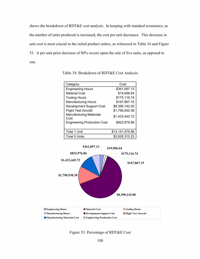
108
shows the breakdown of RDT&E cost analysis. In keeping with standard economics, as
the number of units produced is increased, the cost per unit decreases. This decrease in
unit cost is most crucial in the initial product orders, as witnessed in Table 34 and Figure
53. A per unit price decrease of 80% occurs upon the sale of five units, as opposed to
one.
Table 34: Breakdown of RDT&E Cost Analysis
Category Cost Engineering Hours $361,097.13 Material Cost $19,906.64 Tooling Hours $175,116.74 Manufacturing Hours $167,867.15 Development Support Cost $8,390,142.00 Flight Test Aircraft $1,790,930.38 Manufacturing Materials Cost $1,433,445.72
Engineering Production Cost $822,976.86 Total 1 Unit $13,141,575.98 Total 5 Units $2,628,315.22
$8,390,142.00
$1,790,930.38
$167,867.15
$175,116.74
$361,097.13 $19,906.64$822,976.86
$1,433,445.72
Engineering Hours Material Cost Tooling Hours
Manufacturing Hours Development Support Cost Flight Test Aircraft
Manufacturing Materials Cost Engineering Production Cost
Figure 53: Percentage of RDT&E Cost
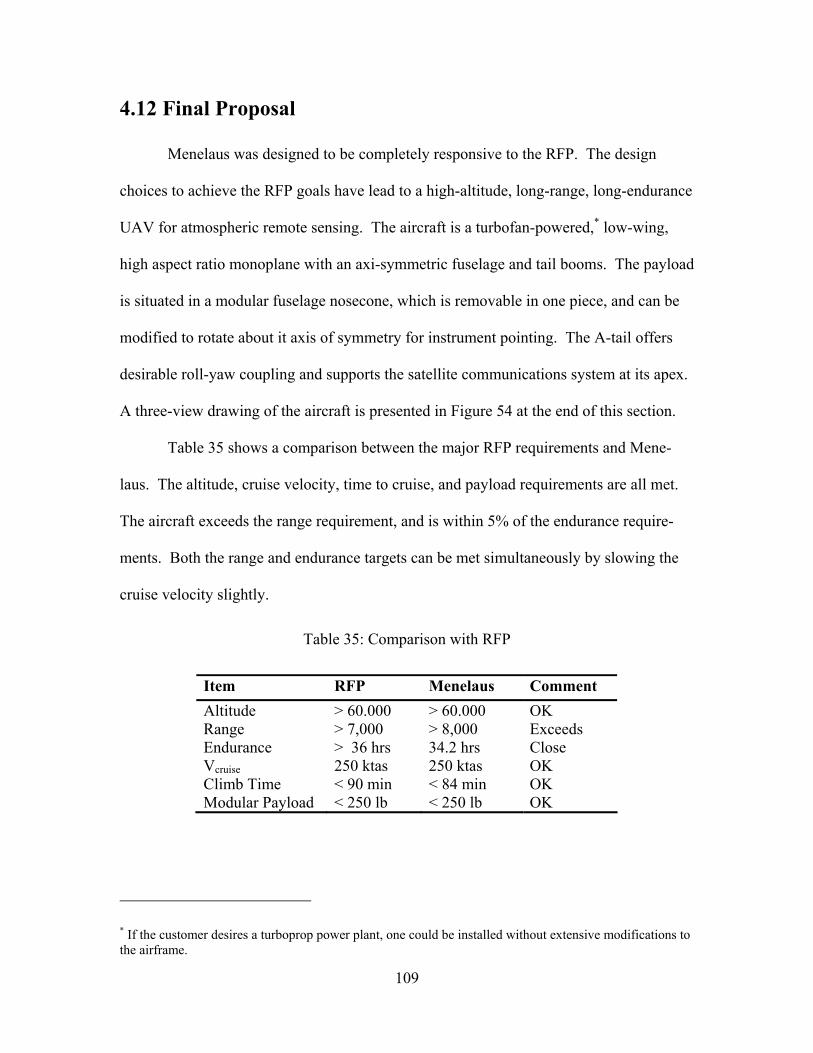
109
4.12 Final Proposal
Menelaus was designed to be completely responsive to the RFP. The design
choices to achieve the RFP goals have lead to a high-altitude, long-range, long-endurance
UAV for atmospheric remote sensing. The aircraft is a turbofan-powered,* low-wing,
high aspect ratio monoplane with an axi-symmetric fuselage and tail booms. The payload
is situated in a modular fuselage nosecone, which is removable in one piece, and can be
modified to rotate about it axis of symmetry for instrument pointing. The A-tail offers
desirable roll-yaw coupling and supports the satellite communications system at its apex.
A three-view drawing of the aircraft is presented in Figure 54 at the end of this section.
Table 35 shows a comparison between the major RFP requirements and Mene-
laus. The altitude, cruise velocity, time to cruise, and payload requirements are all met.
The aircraft exceeds the range requirement, and is within 5% of the endurance require-
ments. Both the range and endurance targets can be met simultaneously by slowing the
cruise velocity slightly.
Table 35: Comparison with RFP
Item RFP Menelaus Comment
Altitude Range Endurance Vcruise Climb Time Modular Payload
> 60.000 > 7,000 > 36 hrs 250 ktas < 90 min < 250 lb
> 60.000 > 8,000 34.2 hrs 250 ktas < 84 min < 250 lb
OK Exceeds Close OK OK OK
* If the customer desires a turboprop power plant, one could be installed without extensive modifications to the airframe.
110
By meeting or exceeding the RFP requirements, Menelaus achieves all the advan-
tages an aircraft platform has over a space-based platform. These were listed in the RFP
and include the following: lower cost (no launch cost), opportunities for maintenance
(without astronauts), mission flexibility, and payload flexibility. The performance of this
aircraft (altitude, range, endurance) offers scientists new and unique data gathering op-
portunities impossible only a few years ago. The low cost opens up these opportunities to
scientists who cannot afford a space mission with a price tag of at least tens of millions of
dollars. As indicated in the RFP, a need exists for high quality, inexpensive alternative to
space-based atmospheric remote sensing platforms, and Menelaus is the answer.
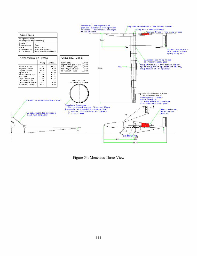
111
Figure 54: Menelaus Three-View
112
Chapter 5: Aiolos
A spacecraft carrying the MicroMAPS instrument would likely be built and oper-
ated by NASA or by contractors working with the agency. In this situation, the possibil-
ity exists that NASA would choose to design a spacecraft platform that would conduct
several science missions from orbit around the Earth. The spacecraft designed for this
project, however, is to carry only one science instrument (MicroMAPS). Such a design
leads to the assumption that the mission would have a relatively small budget, making
cost a significant driver in the design process. As explained in the following sections, the
attempt to reduce cost impacts major decisions such as not including a propulsion system,
launching as a secondary payload, and minimizing the amount of redundancy in the
spacecraft systems. The spacecraft is named Aiolos after the Greek god of the winds,
since the mission calls for the study of the atmospheric transport processes.
5.1 Orbit Design
The science requirements of the MicroMAPS instrument place several restrictions
on the spacecraft orbit design. Since there is only one instrument, formation flying or
constellation missions are not feasible. Due to the nature of the science data, the instru-
ment can only operate from low Earth orbit (LEO). In general, the science mission re-
quires coverage of a high percentage of the Earth’s surface, an indicator that high inclina-
tion orbits should be used.
5.1.1 Specialized Orbits
Two specialized orbits, polar and sun-synchronous, are possibilities for high in-
clinations at LEO. A polar orbit has an inclination of 90° and therefore can take science
113
data over all of the Earth. As discussed later, the primary areas of interest to the science
mission do not include the polar regions. For this reason, the polar orbit is not used so
that a higher percentage of the mission’s lifetime is spent taking useful science data.
The other possible specialized orbit is a sun-synchronous orbit. Due to the effects
of the perturbations on this orbit, the orientation of the orbital plane with respect to the
sun stays constant. Since the spacecraft passes through the orbit’s ascending node at the
same solar time during every orbit, the surface of the Earth can be viewed under consis-
tent lighting conditions. This feature would be useful for MicroMAPS, as the orbit could
be chosen to minimize the interference from clouds in the atmosphere. Yet, this situation
is not optimal for MicroMAPS, as a need exists to understand how carbon monoxide dis-
tribution changes over the course of a day. In addition, a sun-synchronous orbit requires
a propulsion system, which significantly increases the mission cost. Primarily for these
two reasons, the sun-synchronous orbit is not chosen for the Aiolos design.
5.1.2 Propulsion
The inclusion of a spacecraft propulsion system is an important consideration for
orbit design. Propulsion makes orbit control possible, which is advantageous because the
spacecraft could maintain a consistent altitude for the MicroMAPS instrument. A chang-
ing altitude, however, is not a concern as the instrument can compensate for this change
with little impact on the science data.13 A propulsion system also adds considerable cost
to the mission. This cost ranges from $1 million for a huge and heavy cold gas system to
several million dollars for hydrazine, bipropellant, or electic propulsion systems.2 A
propulsion system is not included in the Aiolos design since the science mission benefit
does not justify the cost.
114
5.1.3 Altitude
Aiolos cannot prevent orbital decay without a propulsion system. Orbital decay is
caused by atmospheric drag, eventually causing the spacecraft to burn up in the Earth’s
atmosphere. The most important consideration for the beginning of life (BOL) altitude is
the lifetime desired for the science mission. Since the variation in carbon monoxide data
from one year to another is of interest to scientists, the operational goal for Aiolos is three
years. For this mission, end of life (EOL) is considered to be at an altitude of 300 km.
Designing spacecraft systems to operate below this altitude is impractical and at 300 km,
less than two months remain before the spacecraft burns up in the atmosphere.61 This
mission uses a circular orbit in order to provide approximately consistent viewing condi-
tions for the science instrument throughout a given orbit.
Orbit decay rate (o& ) is determined by Eq. (5.1) where r is the orbit radius, ρ is
atmospheric density, CB is ballistic coefficient and P is the orbit period.
PCro
B
ρπ2
2−=& (5.1) 61
The ballistic coefficient is determined by the physical characteristics of the space-
craft. The orbit radius and period are determined by altitude, and the atmospheric density
is determined by both altitude and the solar cycle. One way to maximize the spacecraft
lifetime at a given altitude is to launch when solar activity is at a minimum. The next
minimum in the solar cycle occurs in 200761, and as such, an ideal launch date for Aiolos
would be June 2007. Table 36 lists the values of atmospheric density at 50 km incre-
ments during minimum solar activity.
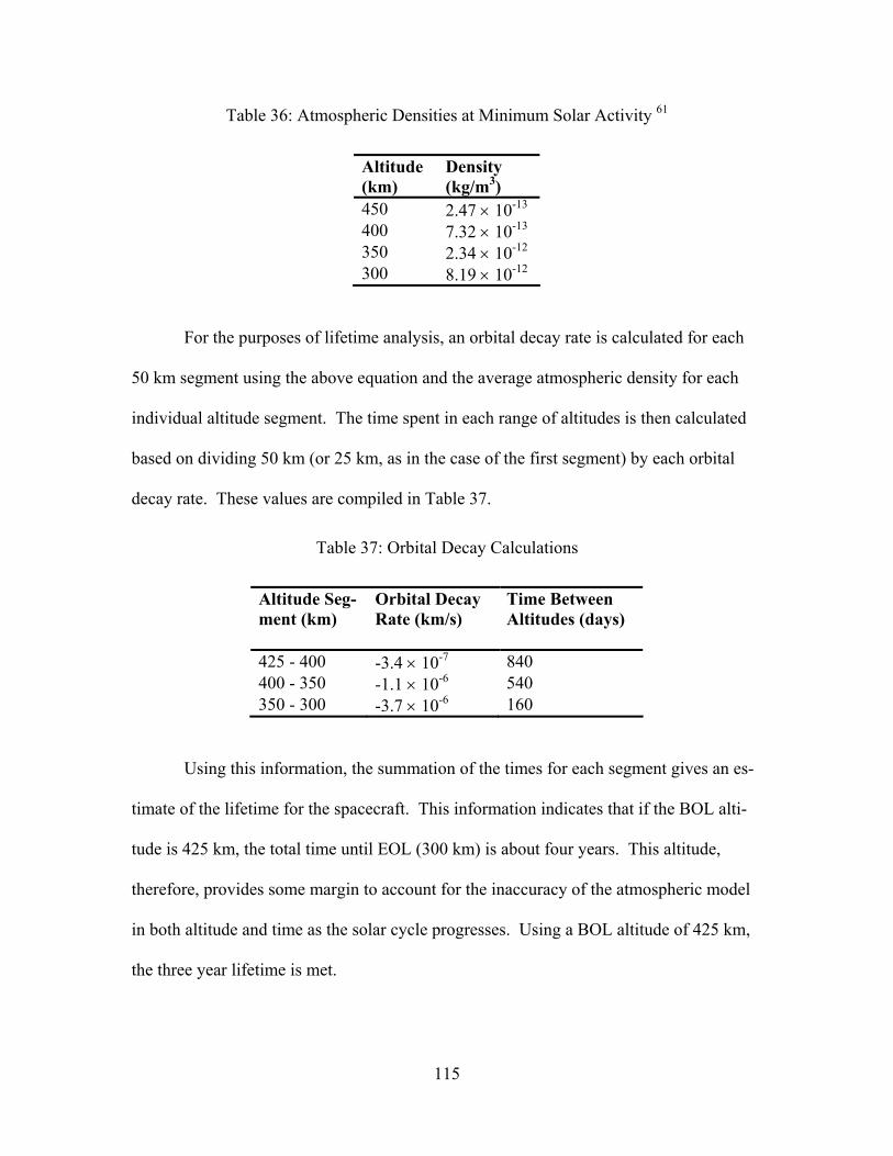
115
Table 36: Atmospheric Densities at Minimum Solar Activity 61
Altitude (km)
Density (kg/m3)
450 2.47 × 10⁻¹³ 400 7.32 × 10⁻¹³ 350 2.34 × 10⁻¹² 300 8.19 × 10⁻¹²
For the purposes of lifetime analysis, an orbital decay rate is calculated for each
50 km segment using the above equation and the average atmospheric density for each
individual altitude segment. The time spent in each range of altitudes is then calculated
based on dividing 50 km (or 25 km, as in the case of the first segment) by each orbital
decay rate. These values are compiled in Table 37.
Table 37: Orbital Decay Calculations
Altitude Seg-ment (km)
Orbital Decay Rate (km/s)
Time Between Altitudes (days)
425 - 400 -3.4 × 10⁻⁷ 840 400 - 350 -1.1 × 10⁻⁶ 540 350 - 300 -3.7 × 10⁻⁶ 160
Using this information, the summation of the times for each segment gives an es-
timate of the lifetime for the spacecraft. This information indicates that if the BOL alti-
tude is 425 km, the total time until EOL (300 km) is about four years. This altitude,
therefore, provides some margin to account for the inaccuracy of the atmospheric model
in both altitude and time as the solar cycle progresses. Using a BOL altitude of 425 km,
the three year lifetime is met.

116
5.1.4 Inclination
Another major component of orbit design is the inclination of the orbit with re-
spect to the equator. This characteristic determines the range of latitudes over which the
MicroMAPS instrument takes science data. The two primary sources of carbon monox-
ide are densely populated, developing countries and biomass burning in various parts of
the world.13 Figure 55 shows population density throughout the world, the densest areas
colored in red.
Figure 55: World Population Density63
The primary transport processes on the Earth move east to west, meaning that
coverage is necessary up to the most extreme latitudes where carbon monoxide produc-
tion is a major concern. As the figure above shows, the most extreme region with a high
population density is Europe, at nearly 60° north latitude. Launching the spacecraft into
an orbit inclined 60° to the equator provides all the necessary coverage for carbon mon-
117
oxide produced from both population density and biomass burning. For the purposes of
launch vehicle selection, the final desired orbit inclination is set at 64°.
5.1.5 Orbit Determination System
Another consideration for orbit design is how orbit determination will be com-
pleted. Historically, most missions have used ground stations or the Tracking and Data
Relay Satellites (TDRS) to track spacecraft. Ground based tracking usually requires sev-
eral orbits and achieves results of several kilometers for LEO.61 The TDRS system pro-
vides nearly complete coverage for LEO with an accuracy on the order of 50 meters.61
This type of system can be used as a backup for Aiolos, but this spacecraft takes advan-
tage of the benefits of a Global Positioning System (GPS) for orbit determination.
Increasing numbers of spacecraft are using GPS for navigation requirements in
LEO. Such a system provides autonomous and real-time orbit determination by provid-
ing the position and velocity of the spacecraft in addition to a highly accurate measure of
the current time. The GPS orbit determination system is an improvement over the accu-
racy of ground based tracking and has low costs.
Surrey Satellite Technology Ltd (SSTL) is a manufacturer of small satellites and
subsystems, including Space GPS Receivers (SGR).48 The SGR-10 model suits the goals
of the Aiolos mission. This receiver includes two antennas that provide position,
velocity, and time measurements. Important data about the SGR-10 is included in Figure
56, and a picture of SGR-20 is shown in Figure 56. The only significant difference
between SGR-10 and SGR-20 is that SGR-20 has four antennas instead of two.
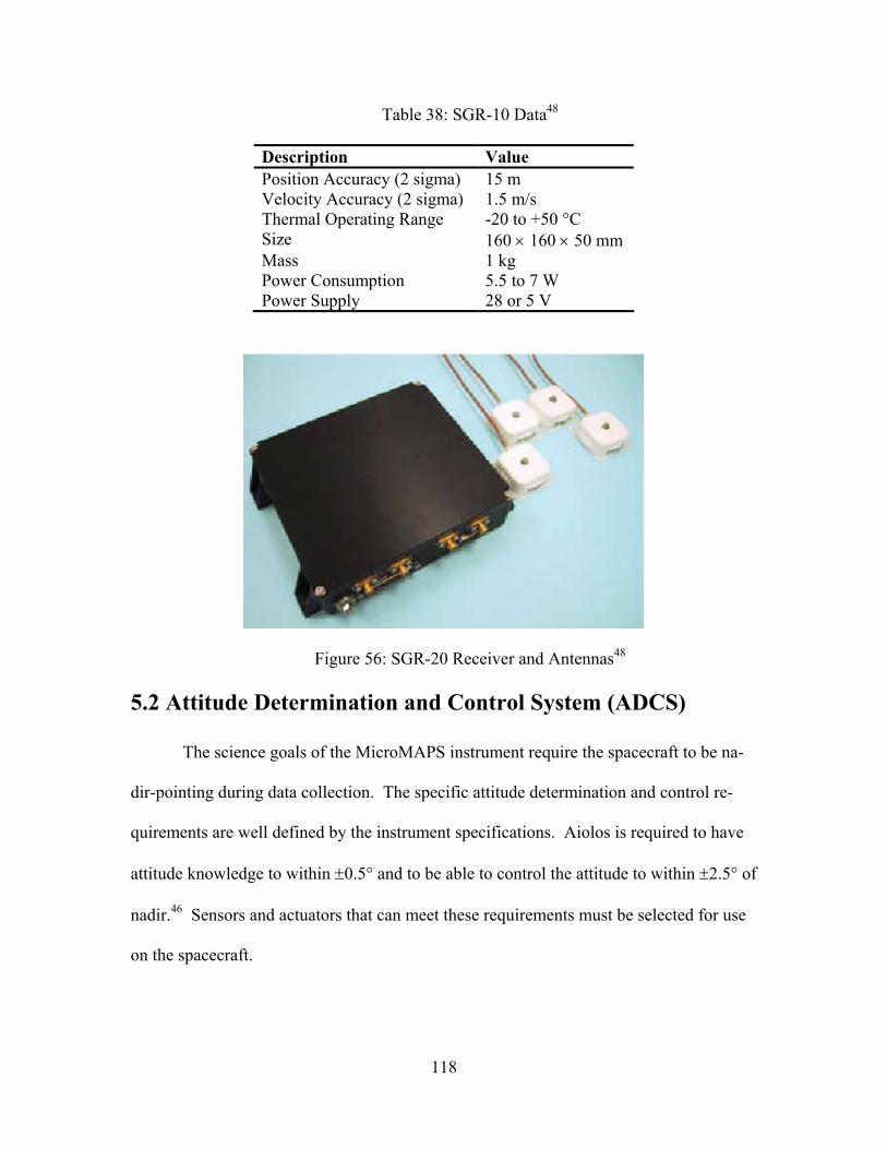
118
Table 38: SGR-10 Data48
Description Value Position Accuracy (2 sigma) 15 m Velocity Accuracy (2 sigma) 1.5 m/s Thermal Operating Range -20 to +50 °C Size 160 × 160 × 50 mm Mass 1 kg Power Consumption 5.5 to 7 W Power Supply 28 or 5 V
Figure 56: SGR-20 Receiver and Antennas48
5.2 Attitude Determination and Control System (ADCS)
The science goals of the MicroMAPS instrument require the spacecraft to be na-
dir-pointing during data collection. The specific attitude determination and control re-
quirements are well defined by the instrument specifications. Aiolos is required to have
attitude knowledge to within ±0.5° and to be able to control the attitude to within ±2.5° of
nadir.46 Sensors and actuators that can meet these requirements must be selected for use
on the spacecraft.
119
Two forms of attitude control systems can be used for a nadir-pointing mission:
gravity-gradient and three axis stabilization.61 Gravity gradient stabilization can only be
the primary method of control for requirements greater than 5°.61 Aiolos, therefore, uses
a three axis primary control scheme but is also configured to take advantage of gravity-
gradient stabilization.
5.2.1 Control Modes
During a mission, ADCS may have several different modes of operation, depend-
ing on the goals of the particular mission segment. These modes can include orbit inser-
tion, acquisition, normal, slew, safe, and special modes.61 Aiolos uses an acquisition
mode to stabilize the vehicle following launch and a safe mode for emergencies on the
spacecraft. The primary mode, however, is the normal mode during which the spacecraft
completes the science mission. The ADCS is designed to operate in this mode through-
out the vast majority of the spacecraft lifetime.
5.2.2 Attitude Determination Components
A wide variety of attitude sensors are typically used on space missions, including
gyroscopes, sun sensors, horizon sensors, star trackers, and magnetometers. Sun sensors,
horizon sensors, and magnetometers are appropriate for this mission due to their rela-
tively low cost, low weight, and high reliability. 61 GPS receivers are also considered, but
attitude determination using GPS is a relatively new concept. Due to the small size of
Aiolos, GPS receivers are unlikely to provide the attitude knowledge needed for this mis-
sion.27
A horizon sensor provides pitch and roll knowledge to the spacecraft. Ithaco
Space Systems builds a Conical Earth Sensor (CES) which meets the requirements of

120
Aiolos. The CES is flight proven, as over 40 of the sensors have been flown on NASA
and DoD missions, demonstrating an accuracy of 0.1°.4 This sensor is vital to the com-
pletion of the Aiolos mission, as it is the primary source for pitch and roll data. Accord-
ingly, two of the sensors are flown on the spacecraft to provide redundancy should one
fail. The CES is shown in instrument information is provided in Table 39.
and instrument information is provided in Table 39.
Figure 57: Ithaco Conical Earth Sensor4
Table 39: Ithaco Conical Earth Sensor Specifications4
Description Value Accuracy 0.1° Size, Sensor Head 9.9d × 11.8 cm Size, Electronics 16.8 × 17.0 × 8.3 cm Mass, Sensor Head 1.1 kg Mass, Electronics 1.9 kg Power Consumption 8 W Input Voltage 22-36 or 31-52 V
For complete attitude determination, knowledge of the third axis, yaw, must be
provided. Aiolos uses sun sensors and a magnetometer to complete the attitude
determination instrument suite. While yaw data are not vital to the science mission, such
information does help to maintain the desired spacecraft orientation throughout the orbit.
Aiolos uses five sun sensors produced by SSTL (Figure 58) as the primary source of yaw

121
data. The two axis sensors provide data for azimuth and elevation to the sun at an
accuracy of 0.5°.48 The five sensors are distributed over the spacecraft to provide data on
the sun’s position while Aiolos is in daylight. This arrangement is designed to maximize
the time that the sun vector is known so that the solar arrays can be most efficient. Data
on the sun sensors are provided in Table 40.
Figure 58: Surrey Two Axis Sun Sensor48
Table 40: Surrey Sun Sensor Specifications48
Description Value Accuracy (Three Sigma) 0.5° Sensor Field of View ± 50° Operating Temperature -50 to 80°C Size 95 × 107 × 35 mm Mass 0.3 kg Power Consumption (sunlit) 100 mW Power Supply ± 12 V
While Aiolos is in eclipse, a magnetometer can be used to determine the yaw
orientation of the spacecraft. Magnetometers do not generally provide the accuracy of a
sun sensor but are particularly useful in conjunction with the magnetic torquers used for
attitude control.61 Ithaco produces a three axis magnetometer, IM-103, that meets the
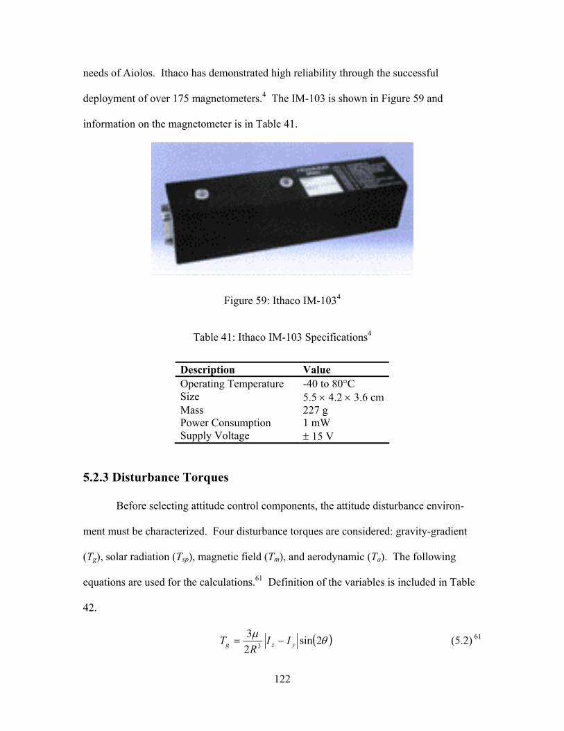
122
needs of Aiolos. Ithaco has demonstrated high reliability through the successful
deployment of over 175 magnetometers.4 The IM-103 is shown in Figure 59 and
information on the magnetometer is in Table 41.
Figure 59: Ithaco IM-1034
Table 41: Ithaco IM-103 Specifications4
Description Value Operating Temperature -40 to 80°C Size 5.5 × 4.2 × 3.6 cmMass 227 g Power Consumption 1 mW Supply Voltage ± 15 V
5.2.3 Disturbance Torques
Before selecting attitude control components, the attitude disturbance environ-
ment must be characterized. Four disturbance torques are considered: gravity-gradient
(Tg), solar radiation (Tsp), magnetic field (Tm), and aerodynamic (Ta). The following
equations are used for the calculations.61 Definition of the variables is included in Table
42.
( )θµ 2sin23
3 yzg IIR
T −= (5.2) 61
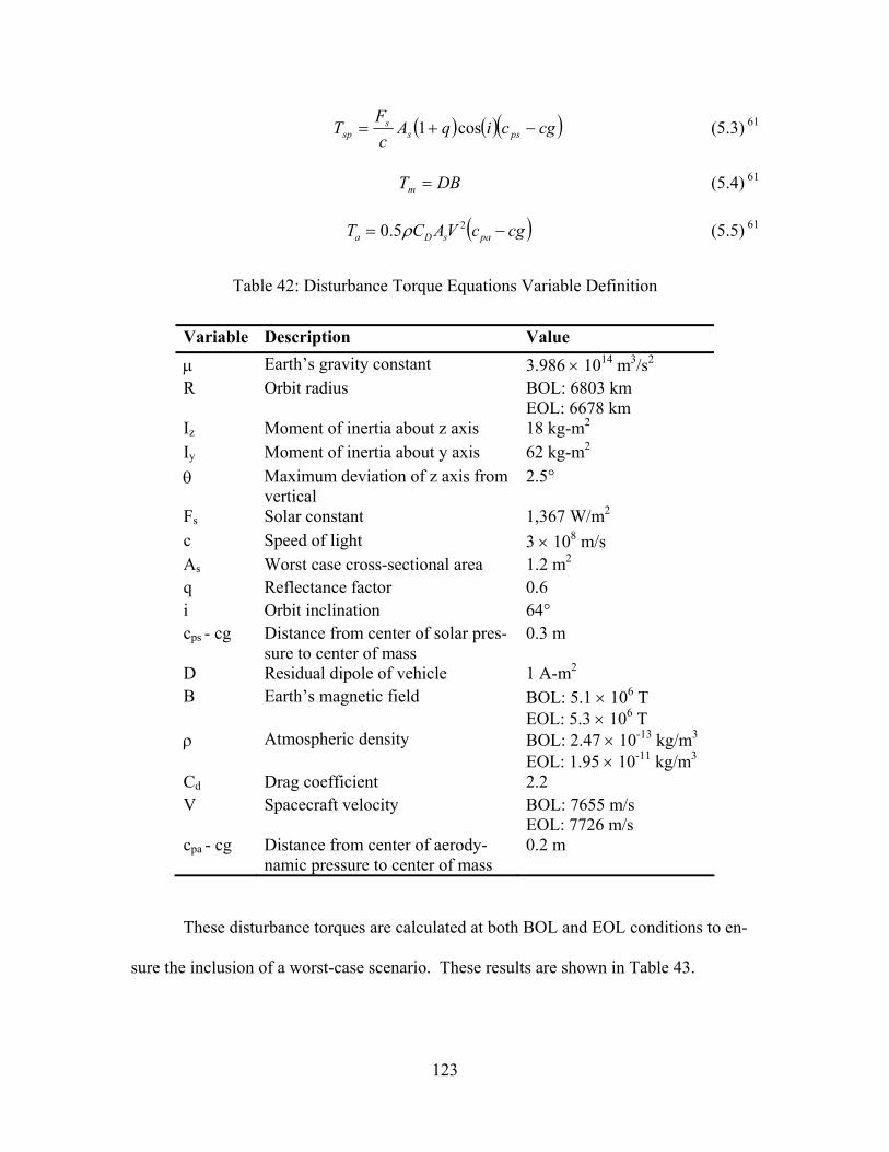
123
( ) ( )( )cgciqAcF
T psss
sp −+= cos1 (5.3) 61
DBTm = (5.4) 61
( )cgcVACT pasDa −= 25.0 ρ (5.5) 61
Table 42: Disturbance Torque Equations Variable Definition
Variable Description Value µ Earth’s gravity constant 3.986 × 10¹⁴ m3/s2 R Orbit radius BOL: 6803 km
EOL: 6678 km Iz Moment of inertia about z axis 18 kg-m2 Iy Moment of inertia about y axis 62 kg-m2 θ Maximum deviation of z axis from
vertical 2.5°
Fs Solar constant 1,367 W/m2 c Speed of light 3 × 10⁸ m/s As Worst case cross-sectional area 1.2 m2 q Reflectance factor 0.6 i Orbit inclination 64° cps - cg Distance from center of solar pres-
sure to center of mass 0.3 m
D Residual dipole of vehicle 1 A-m2 B Earth’s magnetic field BOL: 5.1 × 10⁶ T
EOL: 5.3 × 10⁶ T ρ Atmospheric density BOL: 2.47 × 10⁻¹³ kg/m3
EOL: 1.95 × 10⁻¹¹ kg/m3 Cd Drag coefficient 2.2 V Spacecraft velocity BOL: 7655 m/s
EOL: 7726 m/s cpa - cg Distance from center of aerody-
namic pressure to center of mass 0.2 m
These disturbance torques are calculated at both BOL and EOL conditions to en-
sure the inclusion of a worst-case scenario. These results are shown in Table 43.

124
Table 43: Disturbance Torque Calculations
Torque BOL EOL Gravity-Gradient 7.2 × 10⁻⁶ N-m 7.6 × 10⁻⁶ N-m Solar Radiation 2.6 × 10⁻⁶ N-m 2.6 × 10⁻⁶ N-m Magnetic Field 5.1 × 10⁻⁵ N-m 5.3 × 10⁻⁵ N-m Aerodynamic 3.8 × 10⁻⁶ N-m 3.0 × 10⁻⁴ N-m Total Disturbance Torque 6.4 × 10⁻⁵ N-m 3.7 × 10⁻⁴ N-m
5.2.4 Attitude Control Components
A three axis stabilized system can include many different attitude control actua-
tors, including thrusters, reaction and momentum wheels, control moment gyroscopes,
and magnetic torquers. For Aiolos, thrusters and gyros are not reasonable solutions due
to their high cost and weight. The best solution appears to be a bias momentum wheel
aligned along the pitch axis. The pitch axis is normal to the orbit plane, and such a wheel
allows movement along this axis while stabilizing the other two axes. Magnetic torquer
bars are included to account for attitude drift and to de-saturate the momentum wheel.
The following two equations are used to size the momentum wheel and the magnetic tor-
quers.61
4PTh
a
×=θ
(5.6) 61
BTD = (5.7) 61
In the above equations, h is angular momentum, T is the worst-case disturbance
torque, P is orbital period, θa is allowable motion, D is electrical current, and B is the
Earth’s magnetic field. These values are calculated and shown in Table 44.
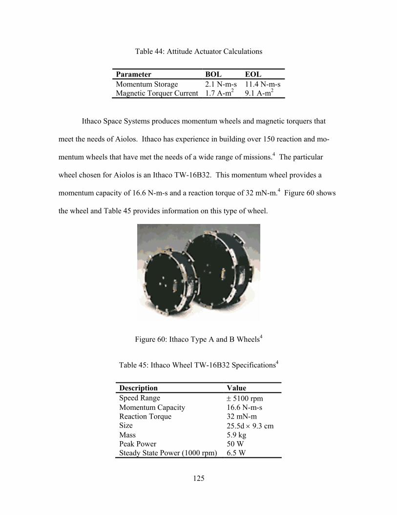
125
Table 44: Attitude Actuator Calculations
Parameter BOL EOL Momentum Storage 2.1 N-m-s 11.4 N-m-s Magnetic Torquer Current 1.7 A-m2 9.1 A-m2
Ithaco Space Systems produces momentum wheels and magnetic torquers that
meet the needs of Aiolos. Ithaco has experience in building over 150 reaction and mo-
mentum wheels that have met the needs of a wide range of missions.4 The particular
wheel chosen for Aiolos is an Ithaco TW-16B32. This momentum wheel provides a
momentum capacity of 16.6 N-m-s and a reaction torque of 32 mN-m.4 Figure 60 shows
the wheel and Table 45 provides information on this type of wheel.
Figure 60: Ithaco Type A and B Wheels4
Table 45: Ithaco Wheel TW-16B32 Specifications4
Description Value Speed Range ± 5100 rpm Momentum Capacity 16.6 N-m-s Reaction Torque 32 mN-m Size 25.5d × 9.3 cm Mass 5.9 kg Peak Power 50 W Steady State Power (1000 rpm) 6.5 W
126
In addition to the wheel, three magnetic torquers are included in Aiolos to provide
the ability to control the attitude about all three axes and to de-saturate the momentum
wheel. Ithaco Space Systems also produces magnetic torquers that fit the requirements of
Aiolos. Three TR10CFR torquers are used, each providing a moment of 12 A-m2. These
torquers are shown in Figure 61 and information is provided in Table 46.
Figure 61: Ithaco Magnetic Torquers4
Table 46: Ithaco Magnetic Torquer TR30CFN Specifications4
Description Value Moment 12 A-m2 Size 1.8d × 38.1 cm Mass 1 kg Power 0.9 W Voltage 15.4 V
5.3 Power
An efficient method of generating, storing, and regulating electric power onboard
the spacecraft is crucial to the success of the mission. The various subsystems are com-
prised of multiple components, all with their own specific power requirements that must
127
be met by the power system. The power generation system on Aiolos converts solar en-
ergy into useable electric energy, which is used to power the spacecraft in daylight. The
energy storage system powers the spacecraft in eclipse and during peak operating condi-
tions. A regulation system is employed to monitor power usage among the various com-
ponents.
5.3.1 Operating Conditions and Requirements
As stated previously, the power subsystem is tasked with providing ample power
to the various spacecraft subsystems when needed. Each component of each subsystem
has its own power and voltage requirements that must be met for optimal operation.
These requirements vary between what is needed on average and what is needed in a
peak condition and are shown in Table 47.
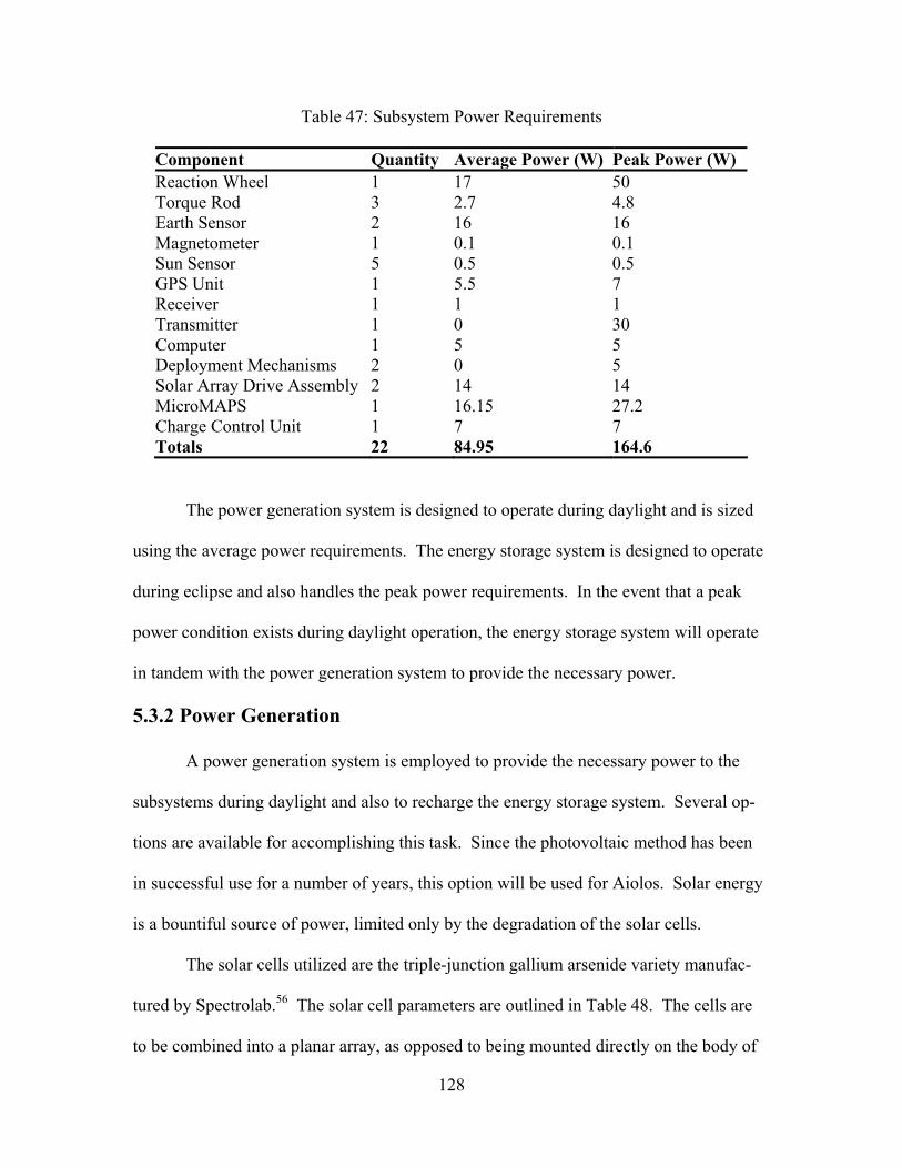
128
Table 47: Subsystem Power Requirements
Component Quantity Average Power (W) Peak Power (W) Reaction Wheel 1 17 50 Torque Rod 3 2.7 4.8 Earth Sensor 2 16 16 Magnetometer 1 0.1 0.1 Sun Sensor 5 0.5 0.5 GPS Unit 1 5.5 7 Receiver 1 1 1 Transmitter 1 0 30 Computer 1 5 5 Deployment Mechanisms 2 0 5 Solar Array Drive Assembly 2 14 14 MicroMAPS 1 16.15 27.2 Charge Control Unit 1 7 7 Totals 22 84.95 164.6
The power generation system is designed to operate during daylight and is sized
using the average power requirements. The energy storage system is designed to operate
during eclipse and also handles the peak power requirements. In the event that a peak
power condition exists during daylight operation, the energy storage system will operate
in tandem with the power generation system to provide the necessary power.
5.3.2 Power Generation
A power generation system is employed to provide the necessary power to the
subsystems during daylight and also to recharge the energy storage system. Several op-
tions are available for accomplishing this task. Since the photovoltaic method has been
in successful use for a number of years, this option will be used for Aiolos. Solar energy
is a bountiful source of power, limited only by the degradation of the solar cells.
The solar cells utilized are the triple-junction gallium arsenide variety manufac-
tured by Spectrolab.56 The solar cell parameters are outlined in Table 48. The cells are
to be combined into a planar array, as opposed to being mounted directly on the body of
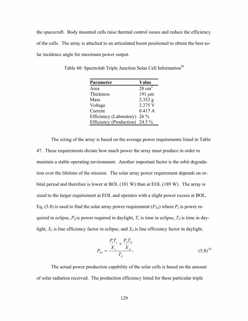
129
the spacecraft. Body mounted cells raise thermal control issues and reduce the efficiency
of the cells. The array is attached to an articulated boom positioned to obtain the best so-
lar incidence angle for maximum power output.
Table 48: Spectrolab Triple Junction Solar Cell Information56
Parameter Value Area 28 cm2 Thickness 191 µm Mass 2.352 g Voltage 2.275 V Current 0.417 A Efficiency (Laboratory) 26 % Efficiency (Production) 24.5 %
The sizing of the array is based on the average power requirements listed in Table
47. These requirements dictate how much power the array must produce in order to
maintain a stable operating environment. Another important factor is the orbit degrada-
tion over the lifetime of the mission. The solar array power requirement depends on or-
bital period and therefore is lower at BOL (181 W) than at EOL (189 W). The array is
sized to the larger requirement at EOL and operates with a slight power excess at BOL.
Eq. (5.8) is used to find the solar array power requirement (PSA) where Pe is power re-
quired in eclipse, Pd is power required in daylight, Te is time in eclipse, Td is time in day-
light, Xe is line efficiency factor in eclipse, and Xd is line efficiency factor in daylight.
d
d
dd
e
ee
SA TX
TPXTP
P+
= (5.8) 61
The actual power production capability of the solar cells is based on the amount
of solar radiation received. The production efficiency listed for these particular triple
130
junction cells is 24.5%.56 Therefore, the ideal power production capability is 335 W/m2,
occurring when the incident solar radiation is normal to the surface of the array. The in-
herent degradation of the cells (a loss of 23%) must be taken into account to find the ac-
tual power production capability at BOL. The incidence angle of the sun must also be
considered, but the array is articulated to achieve a nearly normal incidence angle at all
times. A 10° deviation, however, is assumed to be a worst case scenario, resulting in a
BOL power production capability of 254 W/m2.
Over the course of the mission, the array will degrade so that the capability
achieved at EOL becomes 250 W/m2. The power output is based on the lifetime degrada-
tion of the cells (0.5 % per year) and the duration of the mission (3 years).61 Using the
solar array power requirement and the EOL power production capability, the area of the
array is found to be 0.754 m2. For symmetry purposes, the array area is split between two
small arrays with a total mass of 7.25 kg.
The solar array also must provide the proper bus voltage and current, achieved by
combining the cells into parallel and series strings. The cells are combined into parallel
strings to produce the bus current, and these strings combine in series to produce the bus
voltage.16 Since the entire array is sized according to the conditions at EOL, the individ-
ual strings are designed in the same manner.31 A 28 V bus, the nominal value for most
spacecraft, is desirable. Using this value and the solar array power requirement, the bus
current is computed at 6.7 A. The total number of cells in the array (266) is found using
the array power requirement and the power production capability per cell at EOL. The
number of cells in parallel (19) is found using the bus current and the current provided
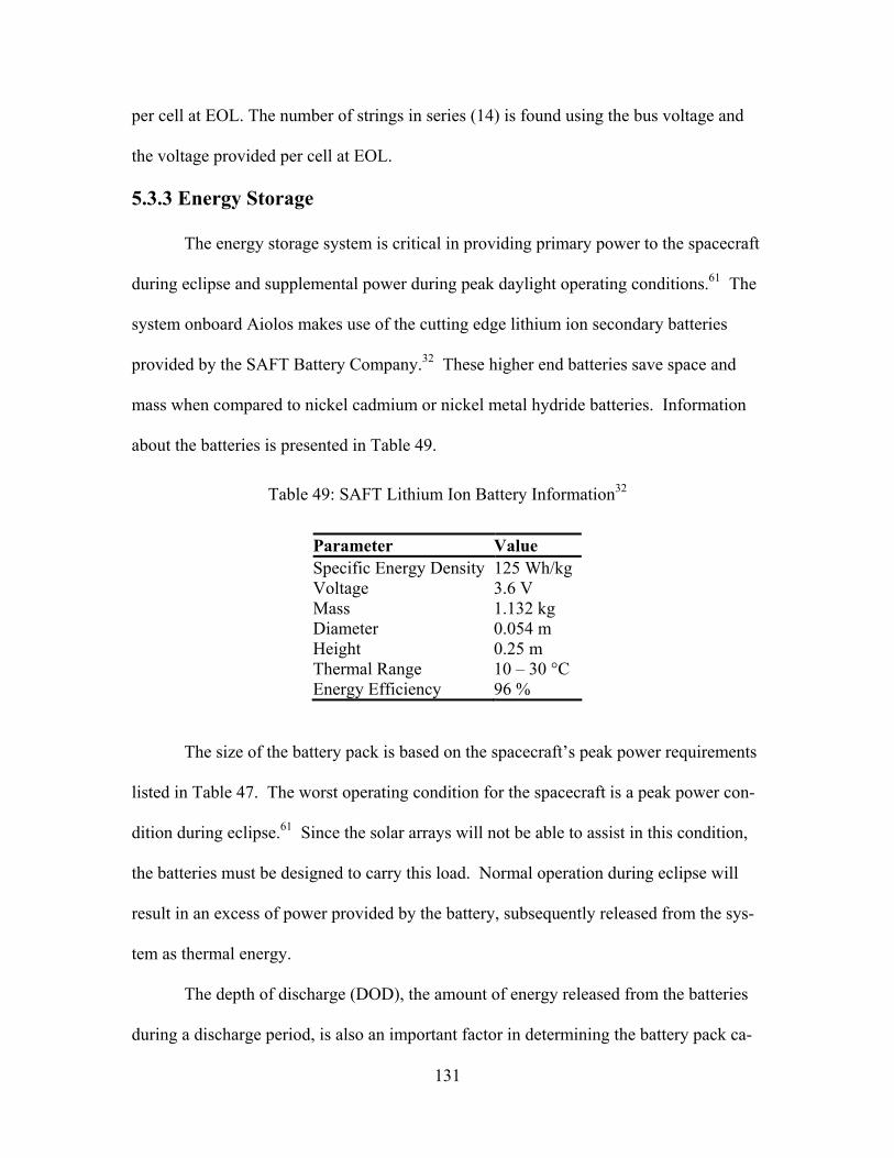
131
per cell at EOL. The number of strings in series (14) is found using the bus voltage and
the voltage provided per cell at EOL.
5.3.3 Energy Storage
The energy storage system is critical in providing primary power to the spacecraft
during eclipse and supplemental power during peak daylight operating conditions.61 The
system onboard Aiolos makes use of the cutting edge lithium ion secondary batteries
provided by the SAFT Battery Company.32 These higher end batteries save space and
mass when compared to nickel cadmium or nickel metal hydride batteries. Information
about the batteries is presented in Table 49.
Table 49: SAFT Lithium Ion Battery Information32
Parameter Value Specific Energy Density 125 Wh/kg Voltage 3.6 V Mass 1.132 kg Diameter 0.054 m Height 0.25 m Thermal Range 10 – 30 °C Energy Efficiency 96 %
The size of the battery pack is based on the spacecraft’s peak power requirements
listed in Table 47. The worst operating condition for the spacecraft is a peak power con-
dition during eclipse.61 Since the solar arrays will not be able to assist in this condition,
the batteries must be designed to carry this load. Normal operation during eclipse will
result in an excess of power provided by the battery, subsequently released from the sys-
tem as thermal energy.
The depth of discharge (DOD), the amount of energy released from the batteries
during a discharge period, is also an important factor in determining the battery pack ca-
132
pacity. A spacecraft operating in LEO experiences about 15 eclipses per day.61 Keeping
the DOD low (in this case, 30%) allows the battery to operate nominally until EOL. The
spacecraft will experience 17,000 eclipse cycles, and this DOD level will be maintained
because the lithium ion batteries preserve their charge better than other battery choices.
The necessary battery capacity is found to be 385 Wh, which can be achieved us-
ing three lithium ion cells in parallel. The battery must also be able to provide and main-
tain the bus voltage of 28 V, therefore requiring eight cells in series. The total pack mass
in this configuration is 17.5 kg, compared to a nickel metal hydride pack with 22 cells
and a mass of 44 kg.
5.4 Command and Data Handling (C&DH)
The primary function of the C&DH subsystem of Aiolos is to store data and to
control the functions of the spacecraft. The data storage requirements include both sci-
ence and telemetry data. The C&DH system stores the data until transmission to a
ground station.
The C&DH system chosen for Aiolos is the OBC 386 on-board data handling sys-
tem made by SSTL.48 The processor is an Intel 386EX running the Posix or SCOS oper-
ating systems with a 25 MHz clockspeed. The system has a 128 MB ramdisk and needs a
28 V potential with a 5 W power supply. No transformer is required since the spacecraft
power subsystem provides the same electrical potential from the solar panels. The sys-
tem weighs 1.7 kg and dimensions are 330 by 330 by 32 mm. This system has long flight
heritage as it has been used on the following spacecraft: FASAT, TMSat, Tsinghua-1,
Tiungsat, and UoSAT-12.
133
The system serves as a central command unit for spacecraft operations. The
communication subsystem, consisting of the transmitter and receiver, is connected to the
C&DH system using two high-speed serial communication channels. Other subsystems
in the spacecraft are connected to the C&DH system via the 10 Mbps Ethernet connec-
tion. The science and telemetry data are stored for later transmission with time flags to
differentiate the data. Interaction between subsystems is also evaluated and controlled by
the computer.
5.5 Communication
The communication subsystem, made up of a transmitter, a receiver, and an an-
tenna, serves as a link between the spacecraft and the ground station. Since the configu-
ration of an antenna depends on its frequency range, a single frequency range used for
both transmitting and receiving would eliminate the need for having two antennas. S-
band frequency, from 2.0 to 4.0 GHz, offers a good choice for the link frequency. Since
the energy of the signal is proportional to the signal frequency, a higher frequency signal
has more energy. For spacecraft to ground communication S-band technologies have a
rich heritage, and many products are available for an S-band communication link. For
these reasons, the S-band frequency is chosen for both uplink and downlink.
5.5.1 Antenna
The antenna chosen is the SSTL S-band Quadrifilar Helix Antenna. The receiv-
ing frequency ranges from 2.01 to 2.10 GHz, and the transmitting frequency ranges from
2.22 to 2.29 GHz. The radiation pattern, shown in Figure 62, is a conical beam with the
maximum gain at the radio horizons.

134
Figure 62: S-band Quadrifilar Helix Antenna Footprint48
The maximum gain configuration of the antenna occurs at each horizon. There-
fore the spacecraft could use the maximum gain opportunity to transmit and receive data
as the ground station enters and exits the footprint. The antenna has a maximum beam
width of 120 degrees with no signal strength at nadir. This beam width translates into a
distance of 1472 km from horizon to horizon in a 425 km orbit. In this orbit, the space-
craft travels at approximately 7.65 km/s, resulting in a total contact duration between the
spacecraft and the ground station of about three minutes. This duration is sufficient due
to the data rate of the transmitter and receiver, discussed in the next few paragraphs.
Physically, the antenna is 100 by 100 by 500 mm and has a mass of 0.5 kg.
5.5.2 Transmitter
The transmitter chosen for Aiolos is the AeroAstro S-band Transmitter with a
transmission range from 2.20 to 2.30 GHz.44 The frequency selected for this mission is
2.25 GHz to counter signal fluctuations and still allow signal transmission. The maxi-
mum output power of the transmitter is 500 mW without an amplifier or a maximum of 5
135
W with the built-in high power amplifier (HPA). This extra power comes at a cost as the
input power requirement increases from 20 W to 30 W, and the mass increases from 180
g to 500 g with the HPA. The voltage is set at 28 V to eliminate the need for a trans-
former. The transmission rate reaches a maximum at 10 Mbps with the HPA in place and
allows a minimum downlink connection time.
MicroMAPS collects 0.45 MB of data per day. Telemetry data depends on sys-
tem activity and is estimated as a maximum of 0.45 MB. Therefore, a maximum of 0.90
MB of data needs to be stored daily. Since the computer can store up to 128 MB of data,
the spacecraft can operate as long as 128 days before requiring an opportunity to trans-
mit. From LEO, Aiolos will be able to contact a ground station much more often than
once every 128 days. Even in this worst case, the spacecraft would only need two sec-
onds to transmit all of its stored data to the ground station.
5.5.3 Receiver
The receiver chosen for Aiolos is the AeroAstro S-band Receiver with a fre-
quency range from 2.025 to 2.120 GHz.44 The frequency is set at 2.060 GHz so that it is
at the center of the range. The data rate which can be received is from 1.0 to 9.6 kbps,
and since the uplink data will only be commands, the data will not be more than a KB.
The data rate set for the receiver is 9.6 kbps since this rate allows the maximum amount
of data to be received.
The uplink sequence starts when the spacecraft is near the horizon, passing out of
the view of the ground station. At this time, a single signal containing the size of the up-
link is received from the ground station. The computer analyzes the signal to determine
when to start the uplink sequence to ensure enough time for the connection. This process
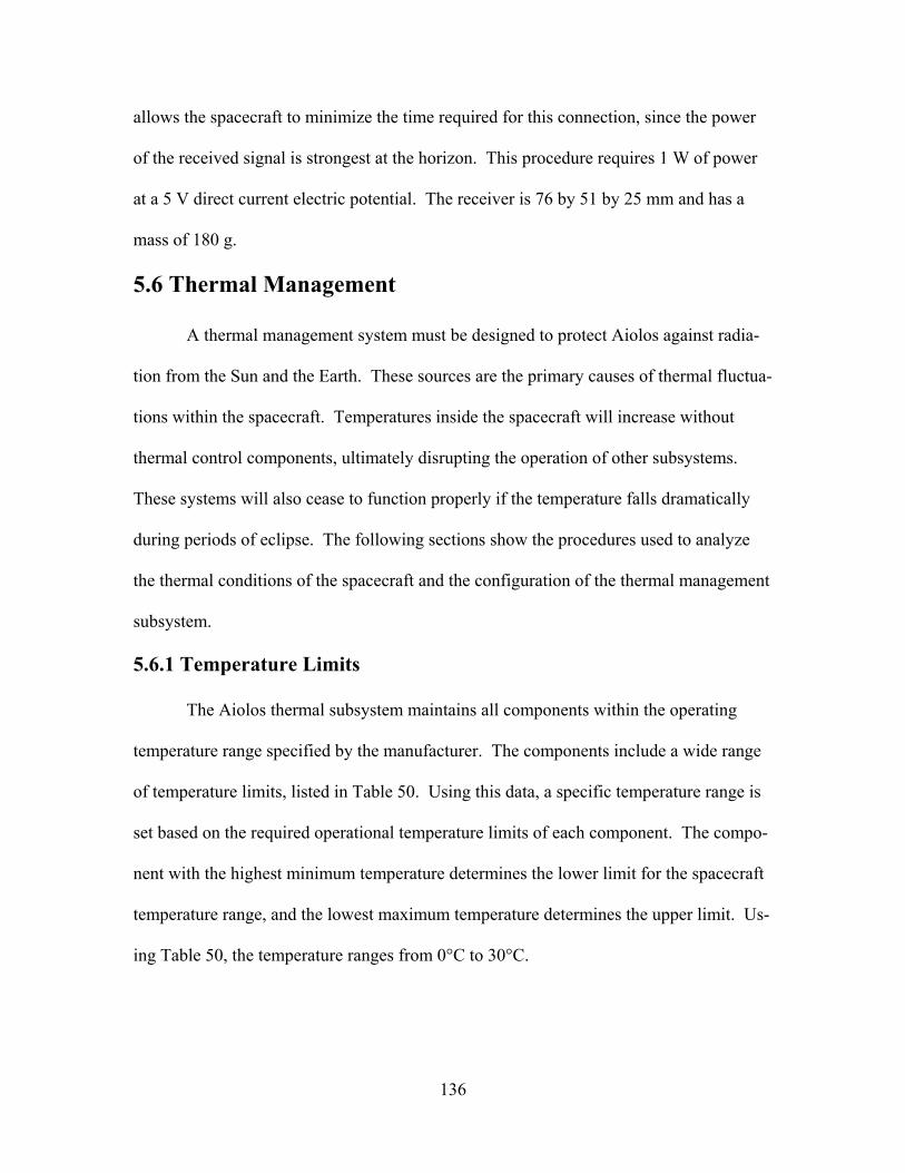
136
allows the spacecraft to minimize the time required for this connection, since the power
of the received signal is strongest at the horizon. This procedure requires 1 W of power
at a 5 V direct current electric potential. The receiver is 76 by 51 by 25 mm and has a
mass of 180 g.
5.6 Thermal Management
A thermal management system must be designed to protect Aiolos against radia-
tion from the Sun and the Earth. These sources are the primary causes of thermal fluctua-
tions within the spacecraft. Temperatures inside the spacecraft will increase without
thermal control components, ultimately disrupting the operation of other subsystems.
These systems will also cease to function properly if the temperature falls dramatically
during periods of eclipse. The following sections show the procedures used to analyze
the thermal conditions of the spacecraft and the configuration of the thermal management
subsystem.
5.6.1 Temperature Limits
The Aiolos thermal subsystem maintains all components within the operating
temperature range specified by the manufacturer. The components include a wide range
of temperature limits, listed in Table 50. Using this data, a specific temperature range is
set based on the required operational temperature limits of each component. The compo-
nent with the highest minimum temperature determines the lower limit for the spacecraft
temperature range, and the lowest maximum temperature determines the upper limit. Us-
ing Table 50, the temperature ranges from 0°C to 30°C.

137
Table 50: Operational Temperature Limit
Component Min. Temp (°C) Max. Temp (°C) MicroMAPS Instrument -6.67 48.9 Ithaco Reaction Wheel -55 70 Ithaco Magnetic Torquer Rods -34 71 Ithaco 3-Axis Magnetometer -20 60 Surrey 2-Axis Sun Sensor -90 90 Computer/Processor -5 50 SSTL S-Band Transmitter -20 50 AeroAstro S-Band Receiver -40 60 SAFT Lithium Ion Batteries 0 30 Aluminum 7075-T73 N/A 532 Aluminized Kapton® (MLI) -269 400
5.6.2 Heat Sources
Two main sources of heat affect Aiolos in LEO: external sources in the environ-
ment and internal heat generated by the subsystems. The external sources include radia-
tion from the Sun and the Earth. In LEO, the radiation received by Aiolos is approxi-
mately equal to the amount of radiation received by the Earth. Solar flux oscillates dur-
ing the year based on the Earth’s orientation with respect to the Sun. An average value of
1353 W/m2 for the solar flux is used in the subsequent analysis.23 The radiation emitted
from the Earth must also be considered, and based on an orbital inclination of 64°, the
Earth emitted radiation ranges from 220 W/m2 to 246 W/m2.23 A third component of ex-
ternal radiation, Earth-reflected solar flux, is called the albedo. Based on the orbital in-
clination, the albedo is 36% of the radiation emitted from Earth.23 Table 51 shows the
environmental fluxes in space.
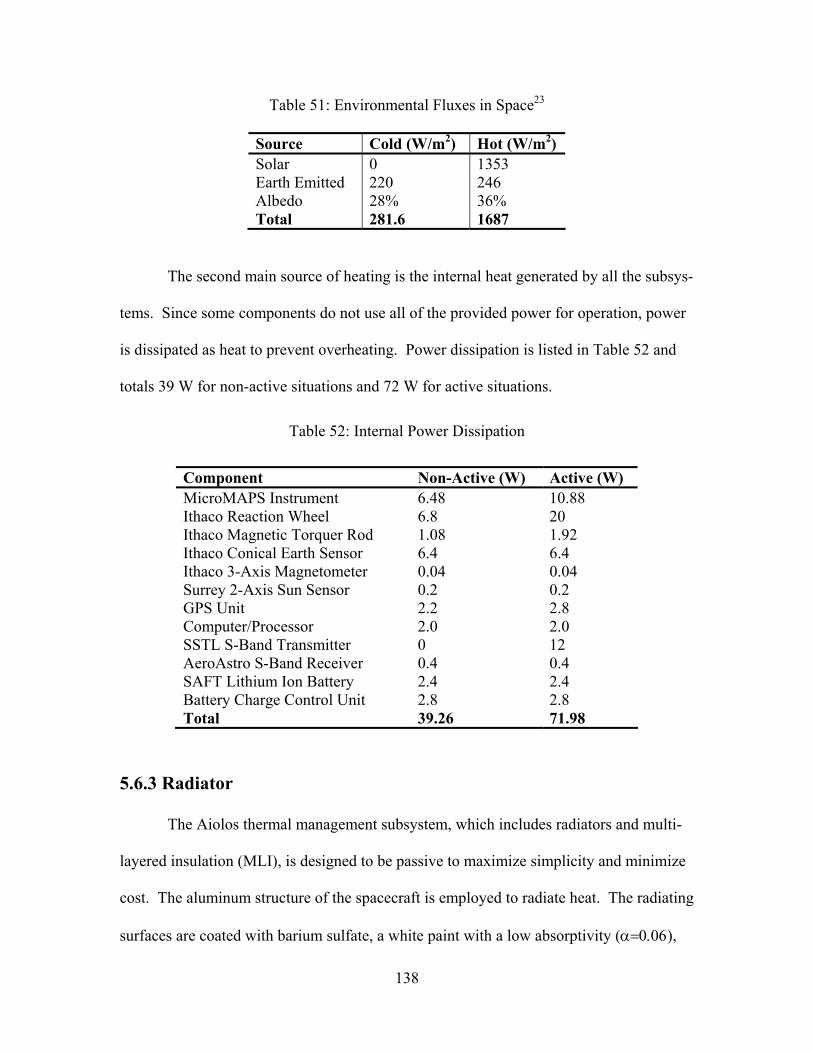
138
Table 51: Environmental Fluxes in Space23
Source Cold (W/m2) Hot (W/m2) Solar 0 1353 Earth Emitted 220 246 Albedo 28% 36% Total 281.6 1687
The second main source of heating is the internal heat generated by all the subsys-
tems. Since some components do not use all of the provided power for operation, power
is dissipated as heat to prevent overheating. Power dissipation is listed in Table 52 and
totals 39 W for non-active situations and 72 W for active situations.
Table 52: Internal Power Dissipation
Component Non-Active (W) Active (W) MicroMAPS Instrument 6.48 10.88 Ithaco Reaction Wheel 6.8 20 Ithaco Magnetic Torquer Rod 1.08 1.92 Ithaco Conical Earth Sensor 6.4 6.4 Ithaco 3-Axis Magnetometer 0.04 0.04 Surrey 2-Axis Sun Sensor 0.2 0.2 GPS Unit 2.2 2.8 Computer/Processor 2.0 2.0 SSTL S-Band Transmitter 0 12 AeroAstro S-Band Receiver 0.4 0.4 SAFT Lithium Ion Battery 2.4 2.4 Battery Charge Control Unit 2.8 2.8 Total 39.26 71.98
5.6.3 Radiator
The Aiolos thermal management subsystem, which includes radiators and multi-
layered insulation (MLI), is designed to be passive to maximize simplicity and minimize
cost. The aluminum structure of the spacecraft is employed to radiate heat. The radiating
surfaces are coated with barium sulfate, a white paint with a low absorptivity (α=0.06),
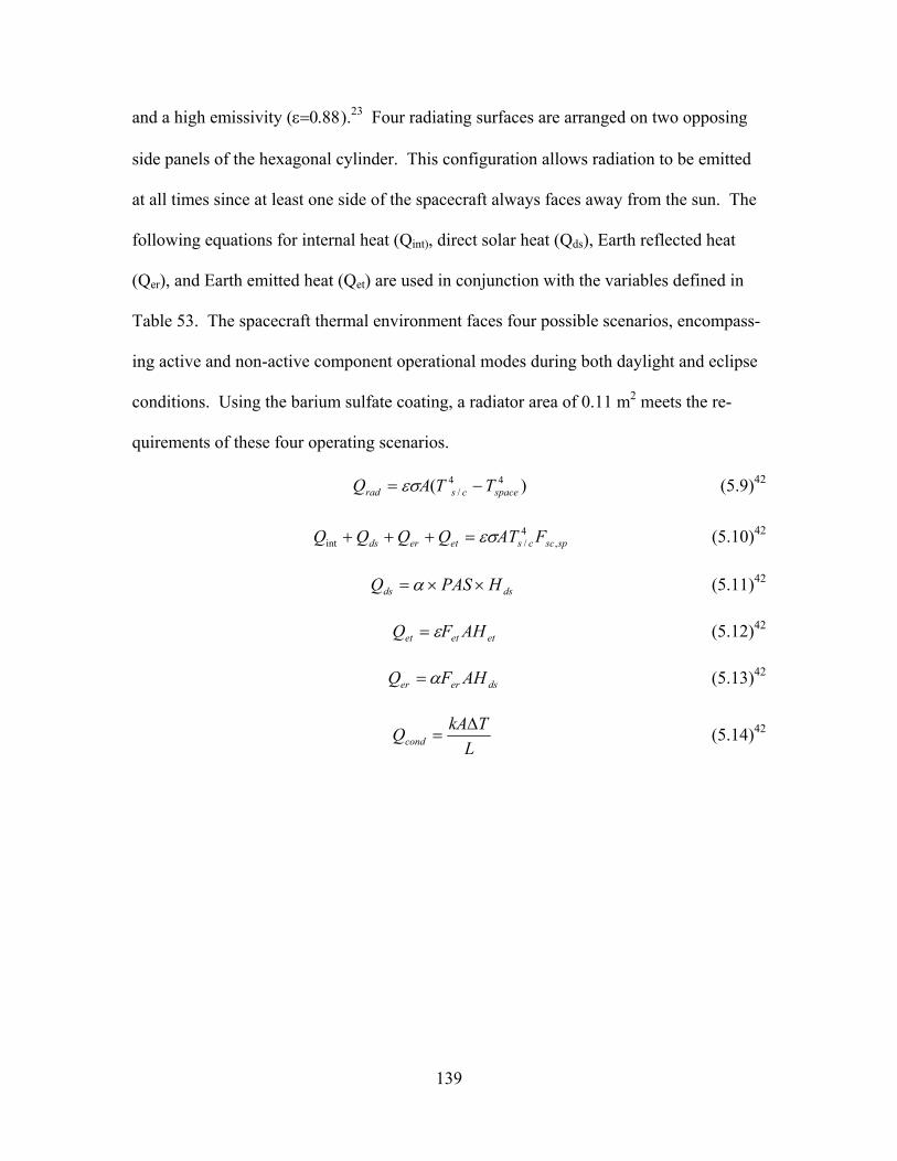
139
and a high emissivity (ε=0.88).23 Four radiating surfaces are arranged on two opposing
side panels of the hexagonal cylinder. This configuration allows radiation to be emitted
at all times since at least one side of the spacecraft always faces away from the sun. The
following equations for internal heat (Qint), direct solar heat (Qds), Earth reflected heat
(Qer), and Earth emitted heat (Qet) are used in conjunction with the variables defined in
Table 53. The spacecraft thermal environment faces four possible scenarios, encompass-
ing active and non-active component operational modes during both daylight and eclipse
conditions. Using the barium sulfate coating, a radiator area of 0.11 m2 meets the re-
quirements of these four operating scenarios.
)( 44/ spacecsrad TTAQ −= εσ (5.9)42
spsccseterds FATQQQQ ,4/int εσ=+++ (5.10)42
dsds HPASQ ××= α (5.11)42
etetet AHFQ ε= (5.12)42
dserer AHFQ α= (5.13)42
LTkAQcond
∆= (5.14)42
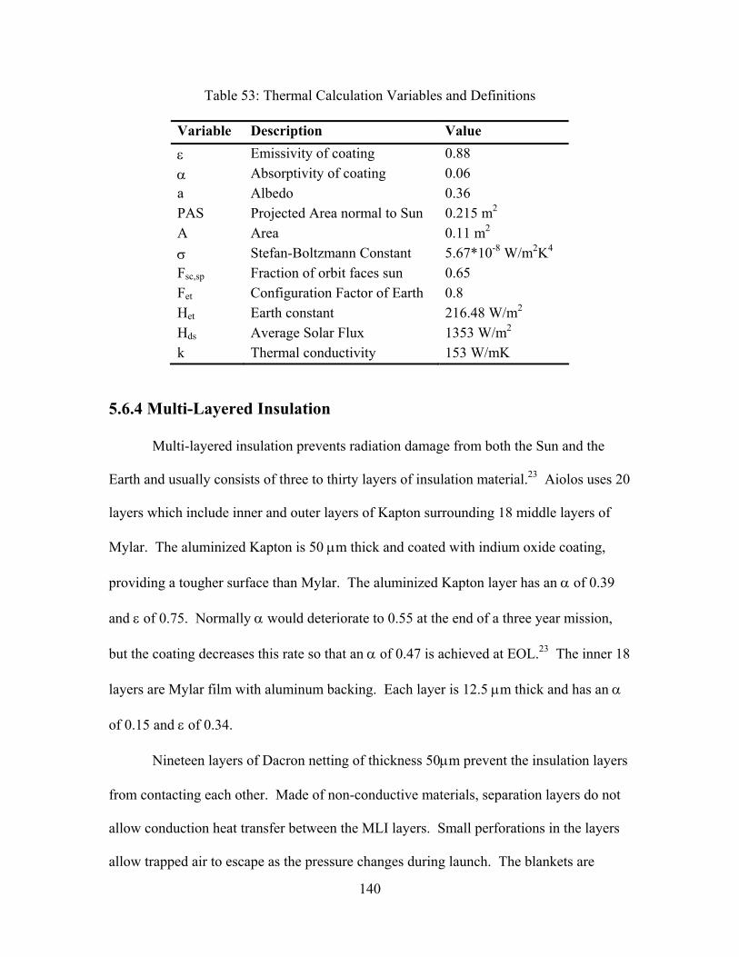
140
Table 53: Thermal Calculation Variables and Definitions
Variable Description Value ε Emissivity of coating 0.88 α Absorptivity of coating 0.06 a Albedo 0.36 PAS Projected Area normal to Sun 0.215 m2 A Area 0.11 m2 σ Stefan-Boltzmann Constant 5.67*10-8 W/m2K4 Fsc,sp Fraction of orbit faces sun 0.65 Fet Configuration Factor of Earth 0.8 Het Earth constant 216.48 W/m2
Hds Average Solar Flux 1353 W/m2 k Thermal conductivity 153 W/mK
5.6.4 Multi-Layered Insulation
Multi-layered insulation prevents radiation damage from both the Sun and the
Earth and usually consists of three to thirty layers of insulation material.23 Aiolos uses 20
layers which include inner and outer layers of Kapton surrounding 18 middle layers of
Mylar. The aluminized Kapton is 50 µm thick and coated with indium oxide coating,
providing a tougher surface than Mylar. The aluminized Kapton layer has an α of 0.39
and ε of 0.75. Normally α would deteriorate to 0.55 at the end of a three year mission,
but the coating decreases this rate so that an α of 0.47 is achieved at EOL.23 The inner 18
layers are Mylar film with aluminum backing. Each layer is 12.5 µm thick and has an α
of 0.15 and ε of 0.34.
Nineteen layers of Dacron netting of thickness 50µm prevent the insulation layers
from contacting each other. Made of non-conductive materials, separation layers do not
allow conduction heat transfer between the MLI layers. Small perforations in the layers
allow trapped air to escape as the pressure changes during launch. The blankets are

141
stitched together around the edges and are attached to the spacecraft using Velcro strips.23
Holes are cut in the insulation to accommodate the radiators, the antenna, the Micro-
MAPS optics, and the solar array drive.
5.7 Launch Vehicle
The orbit design discussed previously heavily influences the launch vehicle selec-
tion. Since this project is a NASA mission, launch vehicle selection is restricted to
United States vehicles and launch sites. In addition, the orbit design requires that the
launch vehicle reach LEO. This requirement eliminates vehicles that primarily launch
geosynchronous transfer orbit (GTO) missions such as Atlas, Delta III and IV, Sea
Launch, and Titan IV. Launching into a high inclination orbit requires the use of launch
sites at either Vandenberg Air Force Base (VAFB) or the Kodiak Launch Complex
(KLC). Due to the size of Aiolos, mass and payload restrictions are not driving factors in
the launch vehicle selection. Structural requirements are considered in Section 5.8. The
most feasible launch vehicles are cheap and reliable and can accommodate the spacecraft
as a secondary payload.
Launching as a secondary payload has several implications for the Aiolos mis-
sion. The desired orbital inclination and altitude may not be attainable, depending on
launch vehicle availability. This design assumes that the launch vehicle can reach the
optimal orbit discussed previously. Aiolos is designed to launch on several vehicles to
improve the number of launch opportunities and to provide competition for the launch
contract.
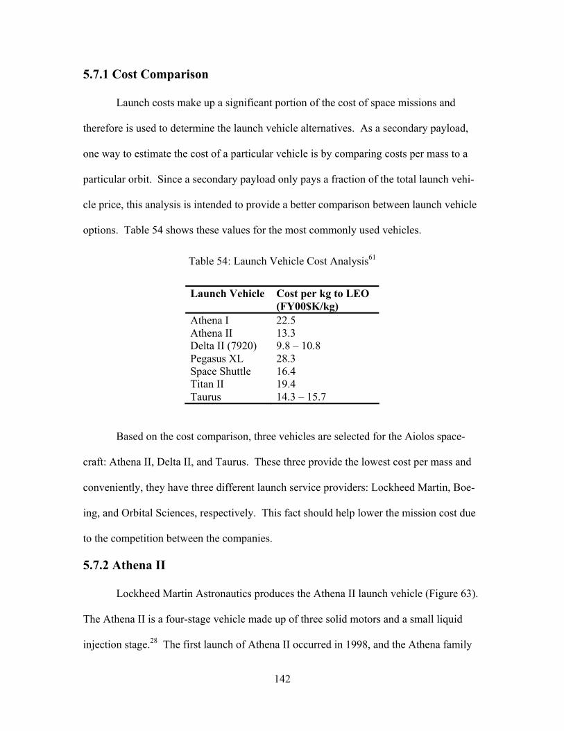
142
5.7.1 Cost Comparison
Launch costs make up a significant portion of the cost of space missions and
therefore is used to determine the launch vehicle alternatives. As a secondary payload,
one way to estimate the cost of a particular vehicle is by comparing costs per mass to a
particular orbit. Since a secondary payload only pays a fraction of the total launch vehi-
cle price, this analysis is intended to provide a better comparison between launch vehicle
options. Table 54 shows these values for the most commonly used vehicles.
Table 54: Launch Vehicle Cost Analysis61
Launch Vehicle Cost per kg to LEO (FY00$K/kg)
Athena I 22.5 Athena II 13.3 Delta II (7920) 9.8 – 10.8 Pegasus XL 28.3 Space Shuttle 16.4 Titan II 19.4 Taurus 14.3 – 15.7
Based on the cost comparison, three vehicles are selected for the Aiolos space-
craft: Athena II, Delta II, and Taurus. These three provide the lowest cost per mass and
conveniently, they have three different launch service providers: Lockheed Martin, Boe-
ing, and Orbital Sciences, respectively. This fact should help lower the mission cost due
to the competition between the companies.
5.7.2 Athena II
Lockheed Martin Astronautics produces the Athena II launch vehicle (Figure 63).
The Athena II is a four-stage vehicle made up of three solid motors and a small liquid
injection stage.28 The first launch of Athena II occurred in 1998, and the Athena family

143
has flown at a rate of 0-2 per year because of relatively low demand.28 Lockheed Martin
reports that a flight rate of at least 10 per year is possible.28 Launch operations from Ko-
diak Launch Complex in Alaska provide a mission inclination range from 64-116°.28
Based on Figure 64, Athena II can carry about 1650 kg to an orbit of 425 km. The pay-
load fairing dimensions are shown in Figure 65.
Figure 63: Athena II Launch Vehicle3
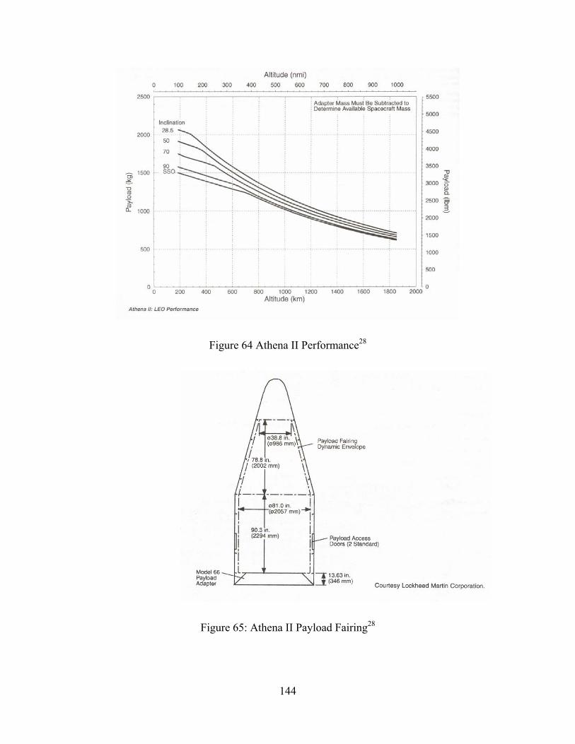
144
Figure 64 Athena II Performance28
Figure 65: Athena II Payload Fairing28
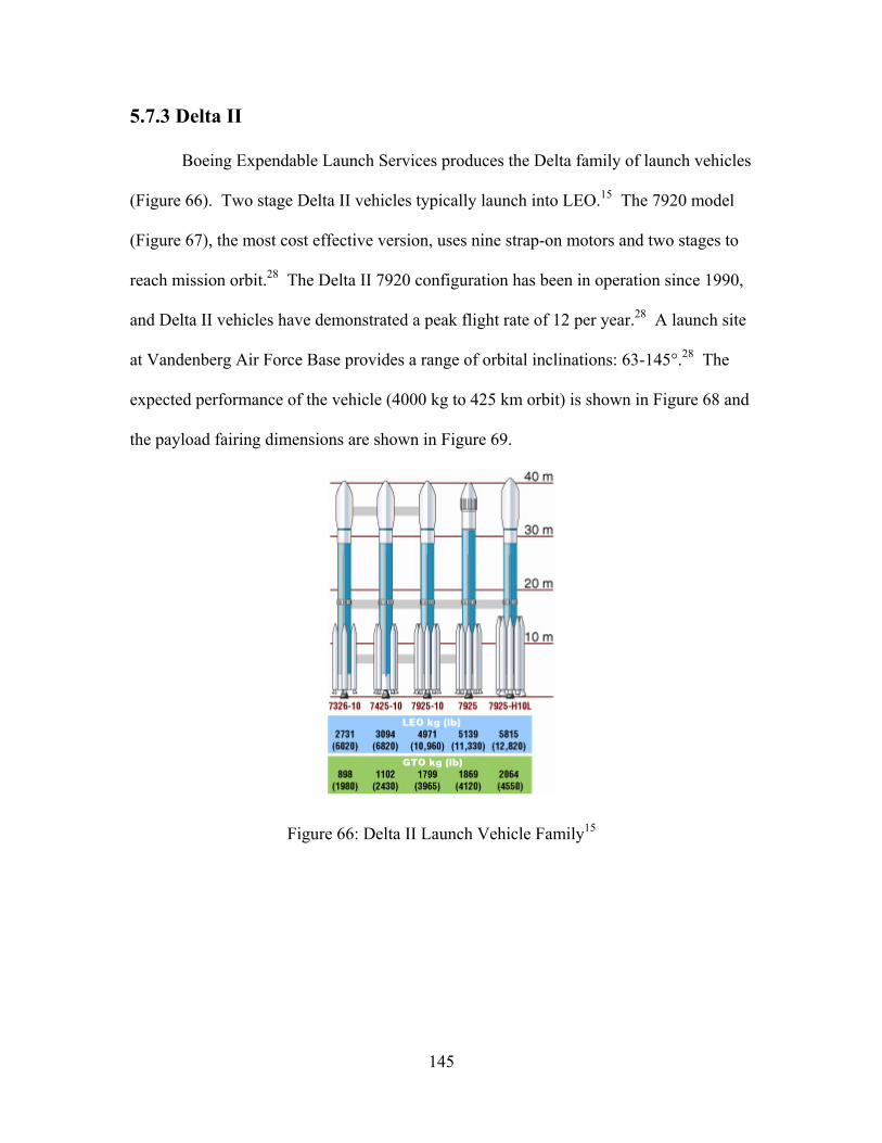
145
5.7.3 Delta II
Boeing Expendable Launch Services produces the Delta family of launch vehicles
(Figure 66). Two stage Delta II vehicles typically launch into LEO.15 The 7920 model
(Figure 67), the most cost effective version, uses nine strap-on motors and two stages to
reach mission orbit.28 The Delta II 7920 configuration has been in operation since 1990,
and Delta II vehicles have demonstrated a peak flight rate of 12 per year.28 A launch site
at Vandenberg Air Force Base provides a range of orbital inclinations: 63-145°.28 The
expected performance of the vehicle (4000 kg to 425 km orbit) is shown in Figure 68 and
the payload fairing dimensions are shown in Figure 69.
Figure 66: Delta II Launch Vehicle Family15
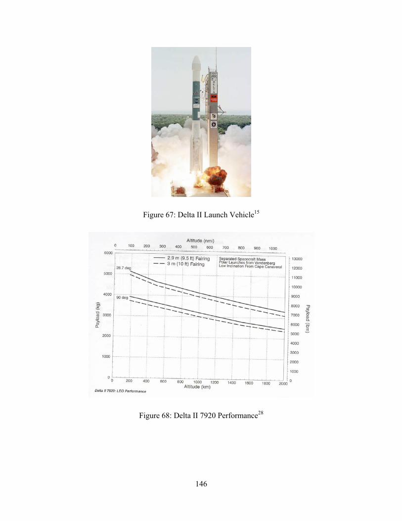
146
Figure 67: Delta II Launch Vehicle15
Figure 68: Delta II 7920 Performance28
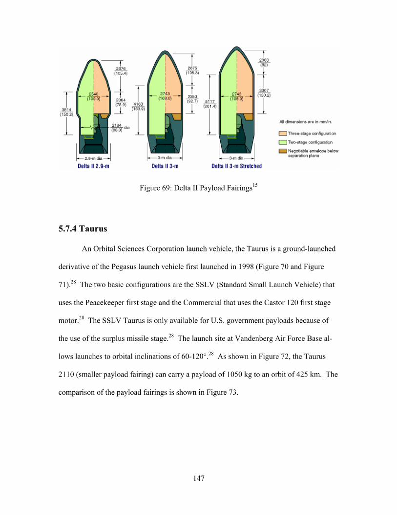
147
Figure 69: Delta II Payload Fairings15
5.7.4 Taurus
An Orbital Sciences Corporation launch vehicle, the Taurus is a ground-launched
derivative of the Pegasus launch vehicle first launched in 1998 (Figure 70 and Figure
71).28 The two basic configurations are the SSLV (Standard Small Launch Vehicle) that
uses the Peacekeeper first stage and the Commercial that uses the Castor 120 first stage
motor.28 The SSLV Taurus is only available for U.S. government payloads because of
the use of the surplus missile stage.28 The launch site at Vandenberg Air Force Base al-
lows launches to orbital inclinations of 60-120°.28 As shown in Figure 72, the Taurus
2110 (smaller payload fairing) can carry a payload of 1050 kg to an orbit of 425 km. The
comparison of the payload fairings is shown in Figure 73.
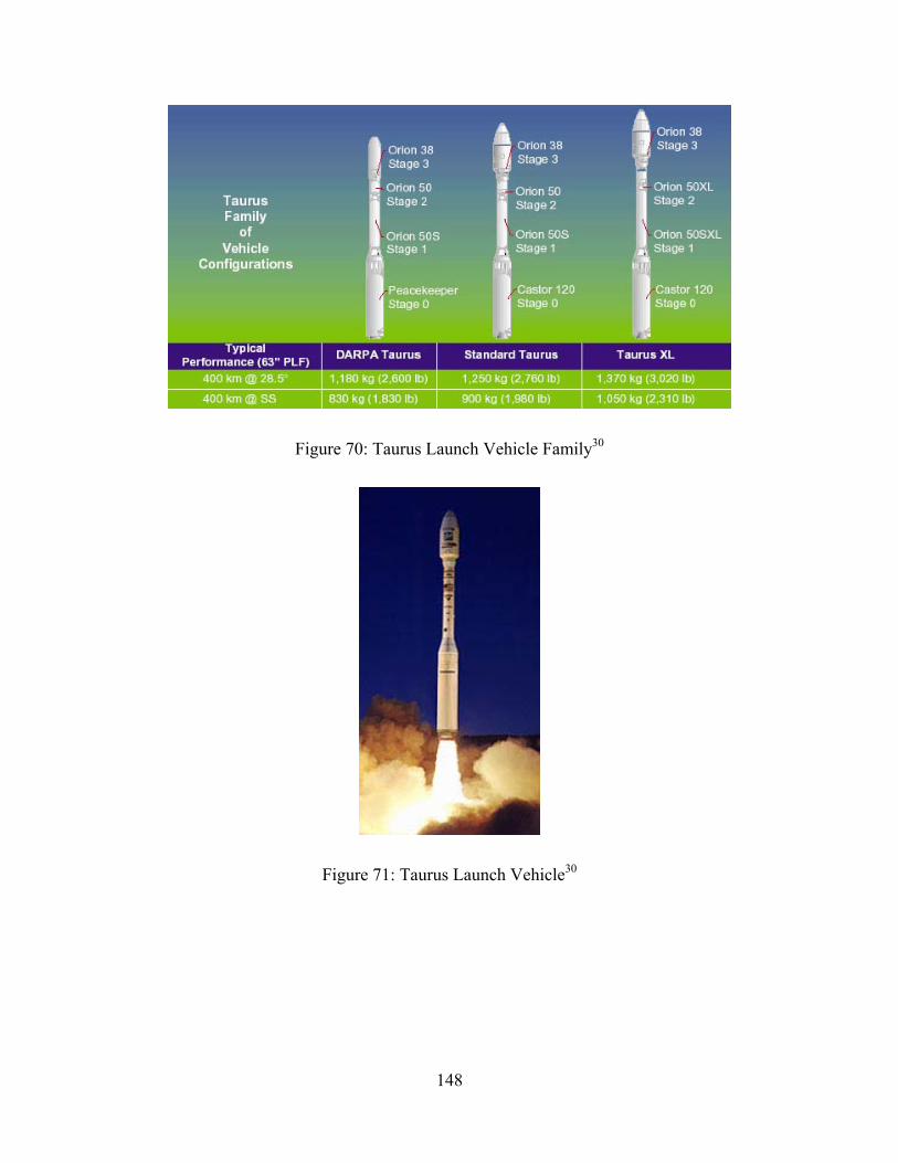
148
Figure 70: Taurus Launch Vehicle Family30
Figure 71: Taurus Launch Vehicle30
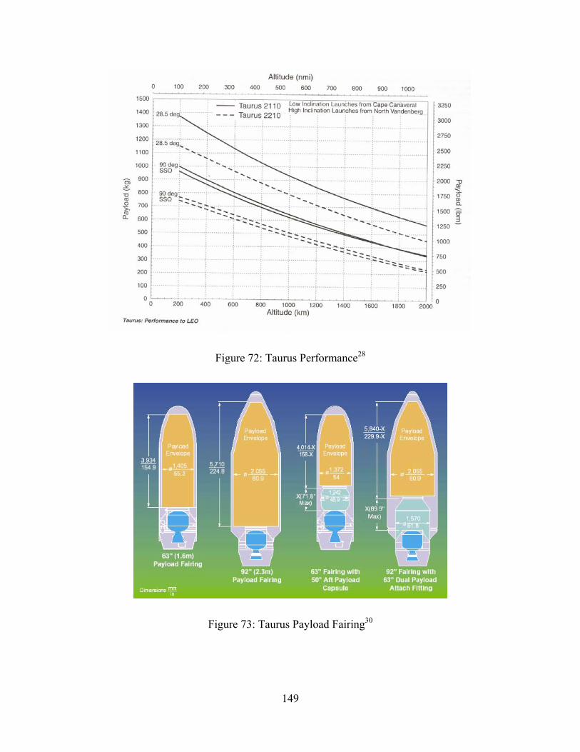
149
Figure 72: Taurus Performance28
Figure 73: Taurus Payload Fairing30

150
5.7.5 Comparison of Options
Aiolos is designed so that it can launch in all three launch vehicle options: Athena
II, Delta II 7920, and Taurus. A listing of parameters relevant to this design is provided
in Table 55.
Table 55: Launch Vehicle Selection Criteria3,15,28,30
Vehicle Athena II Delta II 7920 Taurus Launch Service Provider Lockheed Martin Boeing Orbital SciencesLaunch Site (for 64°) KLC VAFB VAFB Unit Cost ($M) 26 50-55 20-22 Cost per kg to LEO ($K/kg) 13.3 9.8-10.8 14.3-15.7 Flight Record 3/5 103/105 5/6 Flight Rate (units per year) 0-2 10-12 0-2 Payload (to 450 km, 64°) 1650 kg 4000 kg 1050 kg Orbit Injection Accuracy ± 20 km ± 9.3 km ± 29.6 km Payload Fairing 6.1 × 2.3 m 8.49 × 2.9 m 5.5 × 1.6 m Axial Load 8.0 g 6.0 g 8 g Lateral Load 1.8 g 2.5 g 2.5 g Min Longitudinal Frequency 30 Hz 35 Hz 25 Hz Min Lateral Frequency 12 Hz 15 Hz 25 Hz
Although Aiolos is designed to launch in all three vehicles, a need exists to rank
the vehicles based on preference. Several parameters are most important to this decision:
cost, launch environment, reliability, availability, mass to orbit, and payload volume.
Cost is explained previously and is still a factor in the comparison. Launch environment
describes the forces and vibrations the spacecraft will encounter during launch. Reliabil-
ity describes the chance of launch vehicle failure, and availability describes the number
of opportunities to launch. In all cases, Aiolos is well within mass to orbit and payload
volume restrictions, but large values allow more capability for other missions sharing the
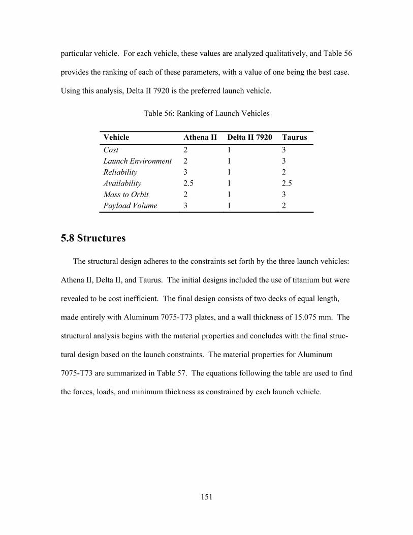
151
particular vehicle. For each vehicle, these values are analyzed qualitatively, and Table 56
provides the ranking of each of these parameters, with a value of one being the best case.
Using this analysis, Delta II 7920 is the preferred launch vehicle.
Table 56: Ranking of Launch Vehicles
Vehicle Athena II Delta II 7920 Taurus Cost 2 1 3 Launch Environment 2 1 3 Reliability 3 1 2 Availability 2.5 1 2.5 Mass to Orbit 2 1 3 Payload Volume 3 1 2
5.8 Structures
The structural design adheres to the constraints set forth by the three launch vehicles:
Athena II, Delta II, and Taurus. The initial designs included the use of titanium but were
revealed to be cost inefficient. The final design consists of two decks of equal length,
made entirely with Aluminum 7075-T73 plates, and a wall thickness of 15.075 mm. The
structural analysis begins with the material properties and concludes with the final struc-
tural design based on the launch constraints. The material properties for Aluminum
7075-T73 are summarized in Table 57. The equations following the table are used to find
the forces, loads, and minimum thickness as constrained by each launch vehicle.
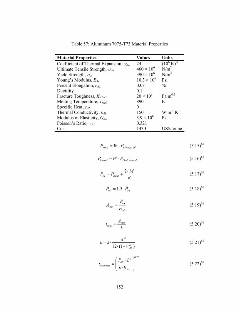
152
Table 57: Aluminum 7075-T73 Material Properties
Material Properties Values Units Coefficient of Thermal Expansion, αAL 24 (106 K)-1
Ultimate Tensile Strength, σult 460 × 106 N/m2
Yield Strength, σys 390 × 106 N/m2
Young’s Modulus, EAL 10.3 × 10⁶ Psi Percent Elongation, eAL 0.08 % Ductility 0.1 Fracture Toughness, KALIC 20 × 106 Pa m0.5 Melting Temperature, Tmelt 890 K Specific Heat, cAL 0 Thermal Conductivity, kAL 150 W m-1 K-1
Modulus of Elasticity, GAL 3.9 × 10⁶ Psi Poisson’s Ratio, νAL 0.321 Cost 1430 US$/tonne
axialLimitaxial PWP ,⋅= (5.15)61
lateralLimitlateral PWP ,⋅= (5.16)61
RMPP axialeq
⋅+=
2 (5.17)61
eqult PP ⋅= 5.1 (5.18)61
ult
eqPA
σ=min (5.19)61
LAt min
min = (5.20)61
)1(12`
2
2
AL
kkν
π−⋅
⋅= (5.21)61
25.02
`
⋅
⋅=
AL
ultbuckling Ek
LPt (5.22)61
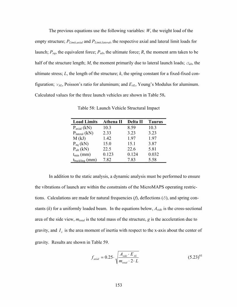
153
The previous equations use the following variables: W, the weight load of the
empty structure; PLimit,axial and PLimit,lateral, the respective axial and lateral limit loads for
launch; Peq, the equivalent force; Pult, the ultimate force; R, the moment arm taken to be
half of the structure length; M, the moment primarily due to lateral launch loads; σult, the
ultimate stress; L, the length of the structure; k, the spring constant for a fixed-fixed con-
figuration; νAL, Poisson’s ratio for aluminum; and EAL, Young’s Modulus for aluminum.
Calculated values for the three launch vehicles are shown in Table 58.
Table 58: Launch Vehicle Structural Impact
Load Limits Athena II Delta II Taurus Paxial (kN) 10.3 8.59 10.3 Plateral (kN) 2.33 3.23 3.23 M (kJ) 1.42 1.97 1.97 Peq (kN) 15.0 15.1 3.87 Pult (kN) 22.5 22.6 5.81 tmin (mm) 0.123 0.124 0.032 tbuckling (mm) 7.82 7.83 5.58
In addition to the static analysis, a dynamic analysis must be performed to ensure
the vibrations of launch are within the constraints of the MicroMAPS operating restric-
tions. Calculations are made for natural frequencies (f), deflections (δ), and spring con-
stants (k) for a uniformly loaded beam. In the equations below, Aside is the cross-sectional
area of the side view, mtotal is the total mass of the structure, g is the acceleration due to
gravity, and xI is the area moment of inertia with respect to the x-axis about the center of
gravity. Results are shown in Table 59.
LmEA
ftotal
ALsideaxial ⋅⋅
⋅⋅=
225.0 (5.23)61
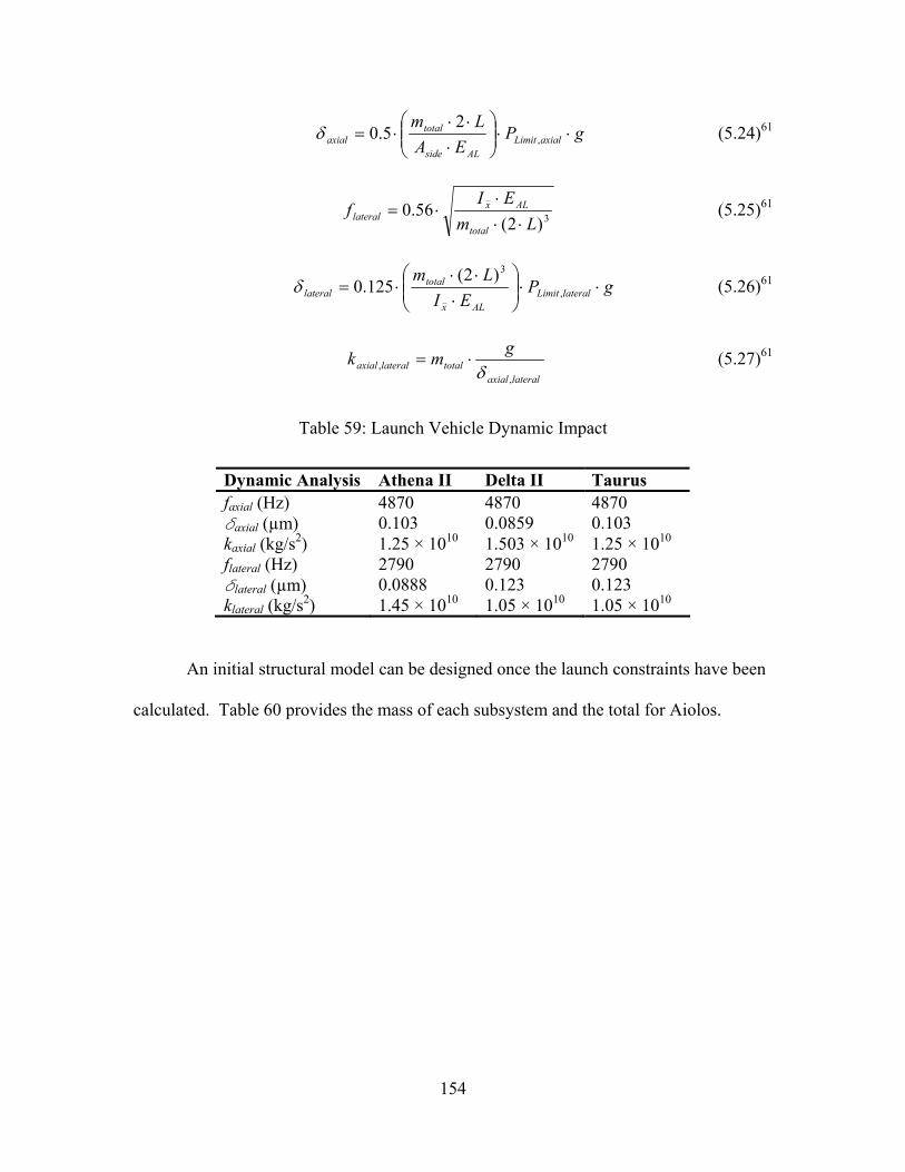
154
gPEA
LmaxialLimit
ALside
totalaxial ⋅⋅
⋅
⋅⋅⋅= ,
25.0δ (5.24)61
3)2(56.0
LmEI
ftotal
ALxlateral ⋅⋅
⋅⋅= (5.25)61
gPEI
LmlateralLimit
ALx
totallateral ⋅⋅
⋅
⋅⋅⋅= ,
3)2(125.0δ (5.26)61
lateralaxialtotallateralaxial
gmk,
, δ⋅= (5.27)61
Table 59: Launch Vehicle Dynamic Impact
Dynamic Analysis Athena II Delta II Taurus faxial (Hz) 4870 4870 4870 δaxial (µm) 0.103 0.0859 0.103 kaxial (kg/s2) 1.25 × 10¹⁰ 1.503 × 10¹⁰ 1.25 × 10¹⁰ flateral (Hz) 2790 2790 2790 δlateral (µm) 0.0888 0.123 0.123 klateral (kg/s2) 1.45 × 10¹⁰ 1.05 × 10¹⁰ 1.05 × 10¹⁰
An initial structural model can be designed once the launch constraints have been
calculated. Table 60 provides the mass of each subsystem and the total for Aiolos.
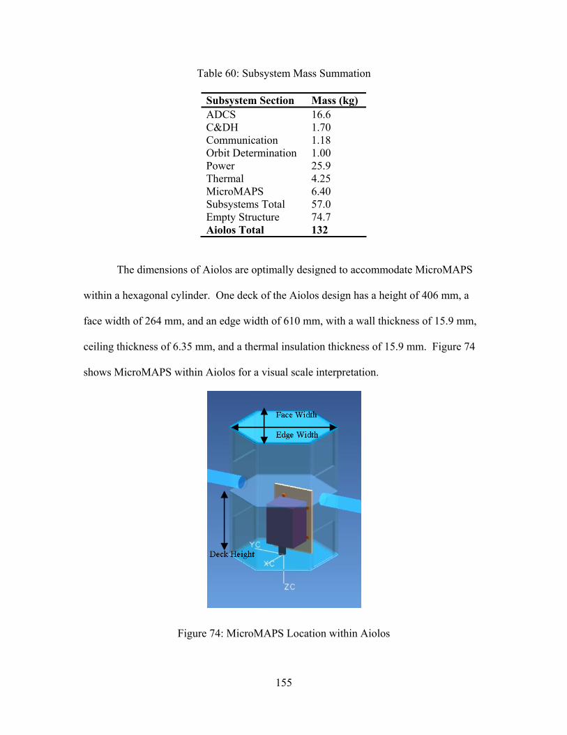
155
Table 60: Subsystem Mass Summation
Subsystem Section Mass (kg) ADCS 16.6 C&DH 1.70 Communication 1.18 Orbit Determination 1.00 Power 25.9 Thermal 4.25 MicroMAPS 6.40 Subsystems Total 57.0 Empty Structure 74.7 Aiolos Total 132
The dimensions of Aiolos are optimally designed to accommodate MicroMAPS
within a hexagonal cylinder. One deck of the Aiolos design has a height of 406 mm, a
face width of 264 mm, and an edge width of 610 mm, with a wall thickness of 15.9 mm,
ceiling thickness of 6.35 mm, and a thermal insulation thickness of 15.9 mm. Figure 74
shows MicroMAPS within Aiolos for a visual scale interpretation.
Figure 74: MicroMAPS Location within Aiolos

156
Subsystems are individually added at specific locations in the structure to mini-
mize the mass and area moments of inertia values. The resulting design is shown in
Figure 75.
Velocity Vector NadirVelocity Vector NadirVelocity Vector Nadir
Figure 75: Complete Aiolos Configuration
The ADCS subsystem is highlighted in red, power is in green, C&DH is in dark
blue, communication is in teal, and MicroMAPS is in purple. The total mass and area
moments of inertia are calculated in Table 61.
Table 61: Inertia Calculations
Moments of Inertia Values Units
XAI 0.0128 m4
YAI 0.0223 m4
ZAI 0.0267 m4
XmI 53.1 kg m2
YmI 61.6 kg m2
ZmI 18.0 kg m2
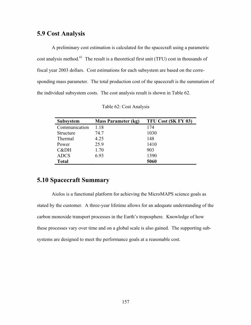
157
5.9 Cost Analysis
A preliminary cost estimation is calculated for the spacecraft using a parametric
cost analysis method.61 The result is a theoretical first unit (TFU) cost in thousands of
fiscal year 2003 dollars. Cost estimations for each subsystem are based on the corre-
sponding mass parameter. The total production cost of the spacecraft is the summation of
the individual subsystem costs. The cost analysis result is shown in Table 62.
Table 62: Cost Analysis
Subsystem Mass Parameter (kg) TFU Cost ($K FY 03) Communication 1.18 174 Structure 74.7 1030 Thermal 4.25 148 Power 25.9 1410 C&DH 1.70 903 ADCS 6.93 1390 Total 5060
5.10 Spacecraft Summary
Aiolos is a functional platform for achieving the MicroMAPS science goals as
stated by the customer. A three-year lifetime allows for an adequate understanding of the
carbon monoxide transport processes in the Earth’s troposphere. Knowledge of how
these processes vary over time and on a global scale is also gained. The supporting sub-
systems are designed to meet the performance goals at a reasonable cost.
158
References
1. “Alaska Aerospace Development Corporation’s Kodiak Launch Complex." Space
Today Online. 8 November 2002.
http://www.spacetoday.org/Rockets/Spaceports/KodiakIsland.html.
2. Asato, D. Propulsion Branch. Guidance, Navigation, and Control Division. NASA
Goddard Space Flight Center. Electronic Mail Correspondence. 14 January 2003.
3. “Athena.” Lockheed Martin Company. 22 March 2003.
http://www.lockheedmartin.com/factsheets/product384.html
4. “Attitude Control Products.” Ithaco Space Systems. 29 March 2003.
http://www.ithaco.com/products.html.
5. Bergquist, A., et al. “Proposed Design for VASCAT.” Design Report. Aerospace
and Ocean Engineering, Virginia Tech. Blacksburg, VA. Spring 2002.
6. Bertin, J. J., and M. L. Smith. Aerodynamics for Engineers. Third Edition. Upper
Saddle River, New Jersey: Prentice Hall, 1998.
7. Bray, B. "Staying Cool on the Space Station". NASA Marshall Space
Flight Center. Huntsville, AL. 14 Oct 2002.
http://liftoff.msfc.nasa.gov/avantgo/stage/news%2Dstationcool.asp.
8. “CB Series 28Vin DC / DC Converters.” Martek Power Abbot, Inc. 2003.
http://www.martekpowerabbott.com.
9. Cengel, Y. A. Introduction to Thermodynamics and Heat Transfer. The McGraw-
Hill Companies, Boston, MA, 1998.
10. Companion, J. A. Virginia Space Grant Consortium. Electronic Mail Correspon-
dence. October 2002 –May 2003.
159
11. “Clark.” JPL Mission and Spacecraft Library Quicklook. 20 September 2002.
http://samadhi.jpl.nasa.gov/msl/QuickLooks/clarkQL.html.
12. Connors, V., Larar, A., Beck, S., and Smith, W., “Proteus Payload.” NASA Goddard
Spaceflight Center. Greenbelt, MD. 12-14 May 1999.
http://eospso.gsfc.nasa.gov/eos_homepage/SAFARI/workshop_links/ptslarar.pdf.
13. Connors, V. NASA Langley Research Center. Informal Conversation. Blacksburg,
VA. 11 February 2003.
14. Dallas Semiconductor. 1 March 2003. http://www.dalsemi.com
15. “Delta.” The Boeing Company. 22 March 2003. http://www.boeing.com/defense-
space/space/delta/flash.html.
16. “Designing a Spacecraft Power System.” Hall, C. D. 20 March 2003.
http://www.aoe.vt.edu/~chall/courses/aoe4065/.
17. Digi-Key Corporation. April 20, 2003. http://www.digikey.com.
18. Doody, D. Basics of Space Flight. Jet Propulsion Laboratory. Pasadena, CA. Feb-
ruary 2001. Available: http://www.jpl.nasa.gov/basics/.
19. “Eclipse Aviation Terminates Contract with Williams International.” Eclipse Avia-
tion. 13 April 2003. http://www.eclipseaviation.com.
20. “engApplets.” W. Davenport, R. Kapania, K. Rojiani, K. Singh, Virginia Tech. 25
April 2003. http://www.engapplets.vt.edu/.
21. Emerson and Cuming. April 22 2003. http://www.emersoncuming.com.
22. Etkin, B., and Reid, L. D. Dynamics of Flight – Stability and Control. Third Edition.
New York: John Wiley & Sons, Inc., 1996.
160
23. Gilmore, D.G. and Bello, M., (editors). Satellite Thermal Control Handbook. The
Aerospace Corporation Press, El Segundo, CA, 1994.
24. Hall, C. D. “Request for Proposal: Air and Space Opportunities for the MicroMAPS
Instrument.” 20 September 2002.
http://www.aoe.vt.edu/~chall/courses/aoe4065/RFPMicroMAPS.pdf.
25. Holman, J.P. Heat Transfer. The McGraw-Hill Companies: New York, NY, 1996.
26. Humble, R.W., G. N. Henry, and W. J. Larson. Space Propulsion Analysis and De-
sign. The McGraw-Hill Companies, 1995.
27. Hwang, Y. “Attitude Determination Using GPS.” 1 November 2002. http://www-
ccar.colorado.edu/~hwangy/gps_atti.htm.
28. Isakowitz, S. J., J. P. Hopkins, and J. B. Hopkins. International Reference Guide to
Space Launch Systems. Third Edition. American Institute of Aeronautics and Astro-
nautics, Reston, VA, 1999.
29. Kutz, M. Temperature Control. John Wiley & Sons, Inc., New York, NY, 1968.
30. “Launch Vehicle Systems.” Orbital Sciences Corporation. Dulles, VA. 8 November
2002. http://www.orbital.com/LaunchVehicle/.
31. Lennox, S. Department of Aerospace and Ocean Engineering. Informal Conversa-
tion. Blacksburg, VA. 27 March 2003.
32. “Lithium Ion Batteries.” SAFT Battery Company. Saft Poitiers, France. 17 March
2002. http://www.saftbatteries.com/130-Catalogue/PDF/space_lithium.pdf.
33. Marchman, J. F. Introductory Aircraft Design. Second Edition. Blacksburg, VA: A-
1 Copies, 2001.
161
34. “MicroMAPS- A Low Cost Orbital Remote Sensor for the Detection of CO and
N2O.” Resonance Ltd. Barrie, Ontario. 31 October 2002.
http://www.resonance.on.ca/mmaps.html.
35. Midon Design. 1 April 2003. http://www.midondesign.com
36. Moreau, M. C. Flight Dynamics Analysis Branch. Guidance, Navigation, and Con-
trol Division. NASA Goddard Space Flight Center. Electronic Mail Correspondence.
November 2002.
37. Morrow, B. Resonance Ltd. Electronic Mail Correspondence. November 2002.
38. “NASA ERAST – A Gateway into Future Aeronautics.” NASA. 2 November 2001.
http://www.dfrc.nasa.gov/Projects/Erast/erast.html.
39. “NASA Facts.” NASA – Dryden Flight Research Center. 15 April 2003.
http://www.dfrc.nasa.gov/Newsroom/FactSheets/index.html.
40. “NASA Terminates Clark Science Mission.” NASA Headquarters Press Release 98-
35. Washington, DC. 25 February 1998.
http://geo.arc.nasa.gov/sge/landsat/clark.html.
41. “NB Series 28Vin DC / DC Converters.” Martek Power Abbot, Inc. 2003.
http://www.martekpowerabbott.com
42. Pisacane, V, L. and Moore, R. C. (editors). Fundamentals of Space Systems. Oxford
University Press, New York, NY, 1994.
43. Point Six, Inc. 10 April 2003. http://www.poinsix.com/cgi-bin/PointSix.cgi?1-Wire
44. “Products and Services.” AeroAstro Inc. Ashburn, VA. 8 April 2003.
http://www.aeroastro.com/products.html.
162
45. Raymer, D. P., ed. Aircraft Design: A Conceptual Approach. Third Edition. Reston,
Virginia: American Institute of Aeronautics and Astronautics, Inc., 1999.
46. Rummell, K. and Walberg, G. “Small Spacecraft Technology Initiative: Measure-
ment of Air Pollution from Satellites (MicroMAPS) Instrument Interface Control
Document.” SSTI-SEIT-014. NASA Contract NASW-4944. 5 May 1995.
47. “SAFT-Space Industry.” SAFT Battery Company. Saft Poitiers, France. 9 Novem-
ber 2002. http://www.saftbatteries.com/space_industry/index.htm.
48. “Satellites and Services.” Surrey Satellite Technology Ltd. 22 March 2003.
http://www.sstl.co.uk/services/subpage_services.html.
49. “Scaled Composites Unveils Proteus, A New High-Altitude, Multi-Mission Aircraft.”
Scaled Composites. Mojave, CA. Updated 23 September 1998.
http://www.scaled.com/projects/proteus/proteus.htm.
50. Schetz, J. A. Boundary Layer Analysis. Upper Saddle, New Jersey: Prentice Hall,
1993.
51. “Software for Aerodynamics and Aircraft Design.” W. H. Mason, Virginia Tech. 15
March 2003. http://www.aoe.vt.edu/~mason/Mason_f/MRsoft.html.
52. “Solar Cells.” Spectrolab, A Boeing Company. Sylmar, CA. 10 November 2002.
http://www.spectrolab.com/prd/prd.asp.
53. Sze, N., Anthropogenic CO emissions: Implications for the atmospheric CO-OH-CH4
cycle, Science, 195673-674 1977.
54. “Tornado: A Vortex lattice MATLAB Implementation for
Linear Aerodynamic Wing Applications.” T. Melin, Royal Institute of Technology

163
KTH, Sweden. 17 February 2003.
http://www.flyg.kth.se/divisions/aero/software/tornado.
55. Tri-M Systems and Engineering. 22 February 2003. http://www.tri-m.com
56. “Triple Junction Solar Cells.” Spectrolab, A Boeing Company. Sylmar, CA. 13
March 2003. http://www.spectrolab.com/DataSheets/TJCell/tj.pdf.
57. “UIUC Airfoil Data Site.” M. Selig, University of Illinois at Urbana-Champaign. 18
March 2003. http://www.aae.uiuc.edu/m-selig/ads.html.
58. U.S. Composite. 22 March 2003. http://www.shopmaninc.com/crbonpage.html.
59. Walberg, G., H. G. Reichle, and W. H. Morrow. “Design and Testing of the Micro-
MAPS Gas Filter Correlation Radiometer.” Final Report SSTI:94C:004. 21 January
1999.
60. “Website for the Defense Industries – Airforce.” Airforce Technology.
http://www.airforce-technology.com/index.html.
61. Wertz, J. R. and Larson, W. J., (editors). Space Mission Analysis and Design. Third
Edition. Microcosm Press and Kluwer Academic Publishers, Boston, 1999.
62. Williams International. 1 April 2003. http://www.williams-int.com/index.htm.
63. “World Population Density.” McGraw-Hill Online Learning Center. 22 March
2003. http://highered.mcgraw-hill.com/sites/007248179x/student_view0/chapter8/
web_map_4.html.