Microbiome Analysis with QIIME2: A Hands-On...
122
Microbiome Analysis with QIIME2: A Hands-On Tutorial Amanda Birmingham Center for Computational Biology & Bioinformatics University of California at San Diego
Transcript of Microbiome Analysis with QIIME2: A Hands-On...

Microbiome Analysis with QIIME2:A Hands-On Tutorial
Amanda BirminghamC e n t e r f o r C o m p u t a t i o n a l B i o l o g y & B i o i n f o r m a t i c sU n i v e r s i t y o f C a l i f o r n i a a t S a n D i e g o

Software Selection• Google “16S analysis <program name>”; main contenders are
•Mothur◦ Name: not an acronym (play on DOTUR, SONS)
◦ Philosophy: single piece of re-implemented software
◦ Top pro: easy to install
◦ Top con: re-implementations could be buggy
◦ Language: C++
◦ Model: open-source
◦ License: GPL
◦ Published: 2009
◦ Developed: at Umichigan

Software Selection• Google “16S analysis <program name>”; main contenders are
• QIIME
◦ Name: Quantitative Insights Into Microbial Ecology
◦ Philosophy: wrapper of best-in-class software
◦ Top pro: extremely flexible
◦ Top con: QIIME 2 not yet feature-complete
◦ Language: python (wrapper)
◦ Model: open-source
◦ License: mixed
◦ Published: 2010
◦ Developed: At UCSD, NAU
Software Selection• Google “16S analysis <program name>”
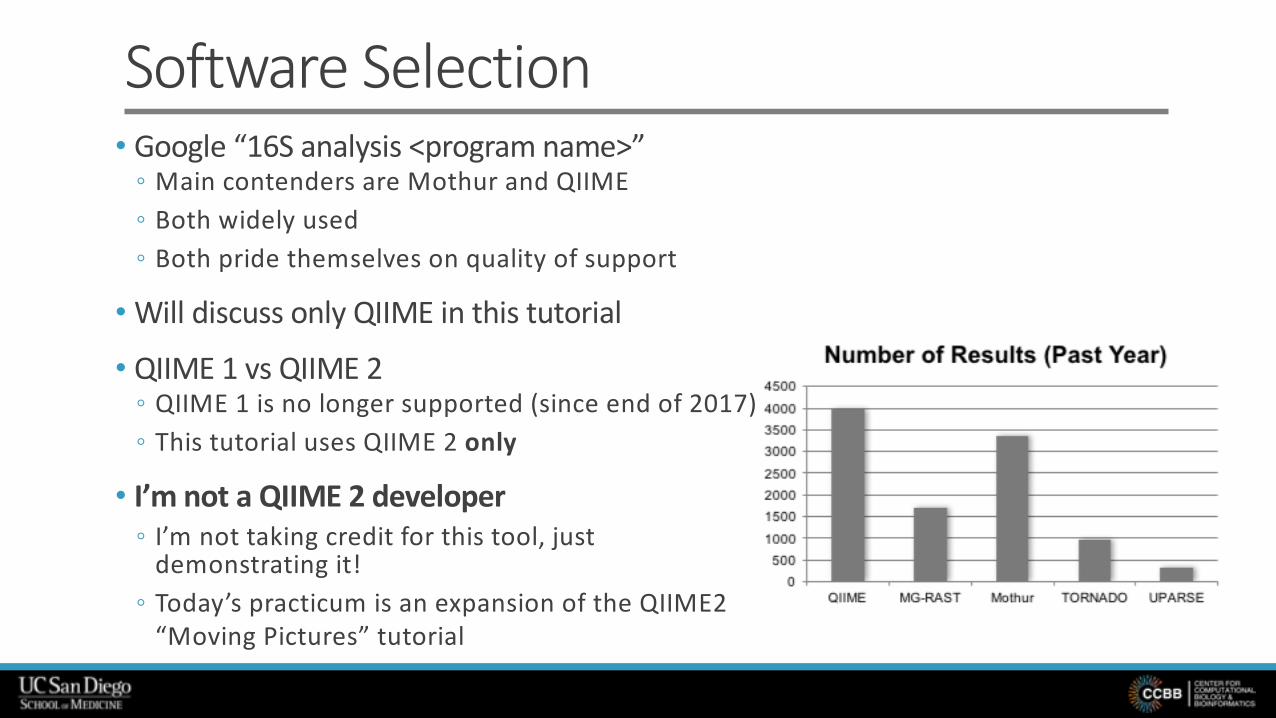
◦ Main contenders are Mothur and QIIME◦ Both widely used◦ Both pride themselves on quality of support
•Will discuss only QIIME in this tutorial
• QIIME 1 vs QIIME 2◦ QIIME 1 is no longer supported (since end of 2017)◦ This tutorial uses QIIME 2 only
• I’m not a QIIME 2 developer◦ I’m not taking credit for this tool, just
demonstrating it!◦ Today’s practicum is an expansion of the QIIME2
“Moving Pictures” tutorial

Prologue: Tuning• Show of hands, please:
◦ How many have analyzed 16S data before?◦ How many know what the “command line” is?◦ How many are comfortable with unix shell commands?

Approach: • Practicum on 16S analysis with QIIME 2
◦ Alternating lecture and tutorial on command-line software
• Suggest you pair up with a partner◦ Two eyes are better than one for finding mistakes and patterns
• Use the provided post-it notes to signal your status◦ None—command not yet completed◦ Green—command completed, no problems◦ Red—having problems!
• Red post-its will be visited by my lovely assistant J

Get Ready To Practice!• “Why are you making me type?!”
◦ QIIME 2 has a GUI—but still under development◦ QIIME 2 command-line interface is easy to install and ready to run◦ Typing is better than copy/pasting commands because in your real analyses, you will
need to type in the appropriate commands for your data§ Need to make realistic typing mistakes now so you know how to correct them later!

Tips to Help•When typing a file name or directory path, you can use tab completion
◦ Start typing file/directory path, then hit tab—if only one file/directory matches what you already typed, shell fills that in§ Very helpful for correctly entering long file names§ If >1 matches, shell fills in as much as it can
• Press up arrow to get back previous commands you typed• If you type a command, press enter, and “nothing happens”, don’t just run it again
◦ Many unix commands produce no visible output to shell—just get back command prompt◦ That doesn’t mean they do nothing, so running them *again* can screw up results◦ Do not store commands in a word processing program (or PowerPoint, etc)§ E.g., MS Word changes hyphens to “m dash”—which command line can’t understand
◦ Shell commands are case-sensitive
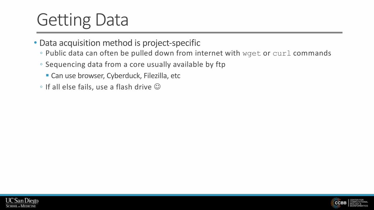
Getting Data• Data acquisition method is project-specific
◦ Public data can often be pulled down from internet with wget or curl commands◦ Sequencing data from a core usually available by ftp§ Can use browser, Cyberduck, Filezilla, etc
◦ If all else fails, use a flash drive J

Getting Data (cont.)• For today’s tutorial, we will use public data from the QIIME2 websitemkdir qiime2-moving-pictures-tutorial
cd qiime2-moving-pictures-tutorial
wget -O "sample-metadata.tsv" \"https://data.qiime2.org/2018.4/tutorials/moving-pictures/sample_metadata.tsv"
mkdir emp-single-end-sequences
wget -O "emp-single-end-sequences/barcodes.fastq.gz" \"https://data.qiime2.org/2018.4/tutorials/moving-pictures/emp-single-end-sequences/barcodes.fastq.gz"
wget -O "emp-single-end-sequences/sequences.fastq.gz" \"https://data.qiime2.org/2018.4/tutorials/moving-pictures/emp-single-end-sequences/sequences.fastq.gz"
wget -O "gg-13-8-99-515-806-nb-classifier.qza" \"https://data.qiime2.org/2018.4/common/gg-13-8-99-515-806-nb-classifier.qza"

Making a Mapping File
• “Mapping file” contains metadata for study◦ Must contain info needed to process sequences and test YOUR hypotheses
• QIIME 1 required certain columns in certain order, but QIIME 2 is more flexible◦ Tab-separated text file with column labels in first line + at least one data line§ Column label values must be unique (i.e. no duplicate values)
◦ First column is the “identifier” column (sample ID)
§ All values in the first column must be unique (i.e. no duplicate values)
◦ See https://docs.qiime2.org/2017.6/tutorials/metadata/
• The easiest way to make a mapping file is with a spreadsheet◦ But Excel is not your friend!§ Routinely corrupts gene symbols, anything interpreted as a dates, etc, & isn’t reversible

Practicum: Viewing A Mapping File• Open Terminal
◦ For below, remember to try tab completion!
◦ Ensure you are in the tutorial directory:
§ qiime2-moving-pictures-tutorial
source activate qiime2-2018.4
ls
nano sample-metadata.tsv
• Stretch the window so you can look at the contents; then, to close, type
Ctrl + x
•Mapping file errors can lead to QIIME 2 errors—or worse, garbage results!
◦ Keemei (pronounced ‘key may’) tool checks for errors in Google Sheets§ Chrome only, and must have Google account to use; see http://keemei.qiime.org/

Mapping File View

Common Issues in Marker Gene Studies• Neglecting metadata
◦ Analysis can not test for effects of, or discard bias from, categories you didn’t record!
• Picking novel 16S primers—not all created equal◦ Earth Microbiome Project recommends 515f-806r primers, error-correcting barcodes
• Not taking precautions to support amplicon sequencing◦ Some Illumina machines require high PhiX, low cluster density
• Selecting an inappropriate reference database◦ E.g., Greengenes (16S) reference database when sequencing ITS
• Expecting species-level taxonomy calls◦ Most sequence variants only specify to family or genus level
• Using inappropriate statistical tests◦ Taxa abundance requires a compositionality-aware test like ANCOM◦ Differences in β diversity distances across groups requires test like PERMANOVA, not ANOVA

Importing Data• After sequence data is on your machine, must be imported to a QIIME 2 “artifact”
◦ Artifact = data + metadata
◦ QIIME 2 artifacts have extension .qza◦ Different kinds of input data (e.g., single-end vs paired-end) and different formats of
input data (e.g., sequences & barcodes in same or different file) need different imports
§ See “Importing data” tutorial at https://docs.qiime2.org/

Practicum: Importing Data
• Backslash is line continuation◦ Could leave out and just type whole command as one run-on line J
• Note structure of arguments to qiime command◦ Plugin name then method name then arguments§ Order matters
qiime tools import \--type EMPSingleEndSequences \--input-path emp-single-end-sequences \--output-path emp-single-end-sequences.qza
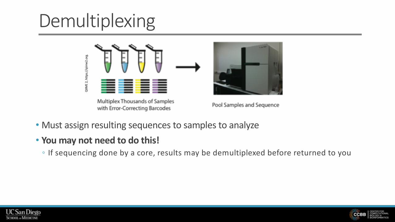
Demultiplexing
•Must assign resulting sequences to samples to analyze • You may not need to do this!
◦ If sequencing done by a core, results may be demultiplexed before returned to you
QIIM
E 2,
http
s://q
iime2
.org
.

Practicum: Demultiplexingqiime demux emp-single \--i-seqs emp-single-end-sequences.qza \--m-barcodes-file sample-metadata.tsv \--m-barcodes-column BarcodeSequence \--o-per-sample-sequences demux.qza
• Arguments have a naming convention◦ Inputs (--i-<whatever>), metadata (--m-<whatever>), parameter (--p-<whatever),
output (--o-<whatever>)◦ Order doesn’t matter

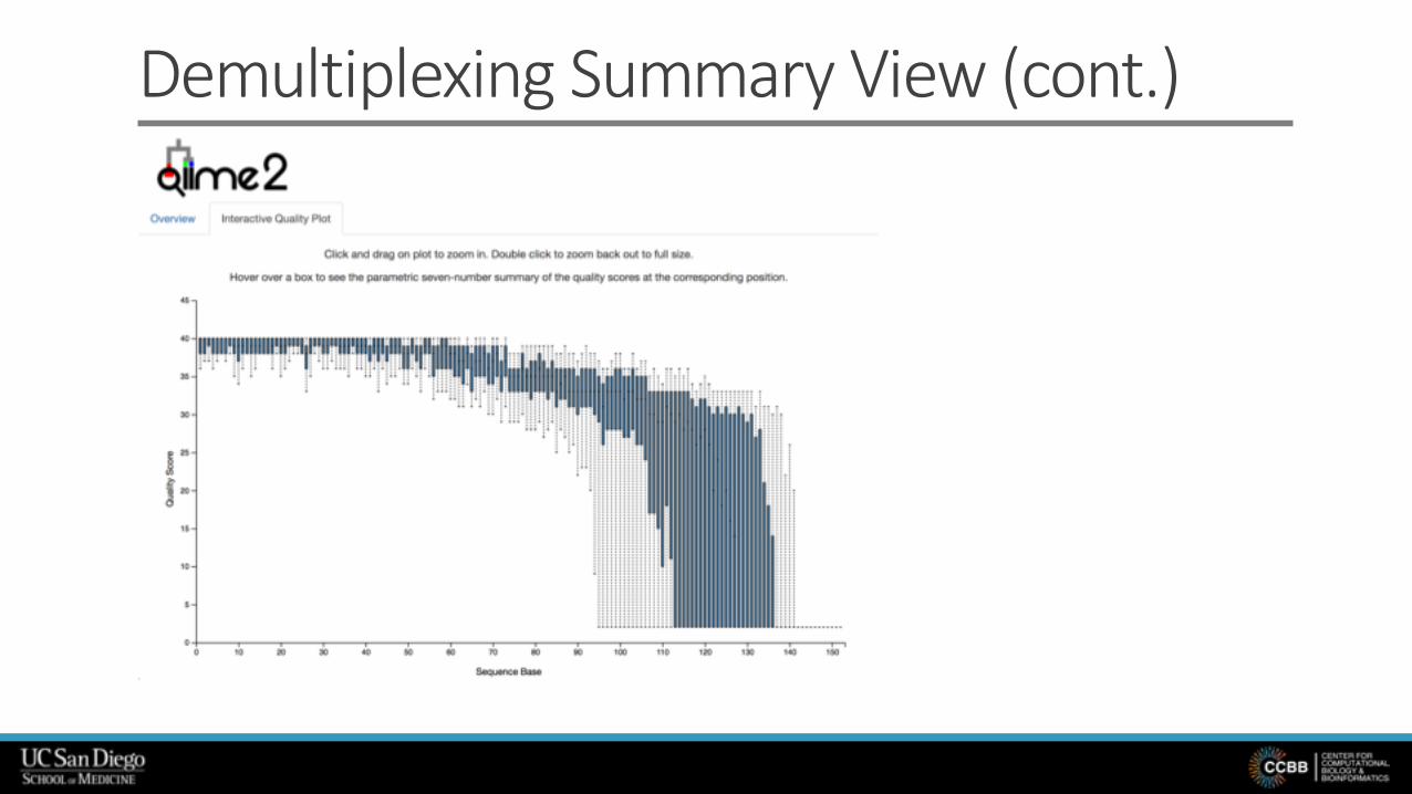
Practicum: Demultiplexing (cont.)• Presumably you’d like to know how your demultiplexing worked• But the artifact doesn’t show you that info, so create a visualization
◦ Note that visualizations have the extension .qzv instead of .qza
• Now view the visualization, locallyqiime tools view demux.qzv
•When done examining, in Terminal, type JUST q◦ Don’t need to hit Enter afterwards◦ Beware: quitting visualization doesn’t close web page (but page becomes unreliable)
qiime demux summarize \--i-data demux.qza \--o-visualization demux.qzv
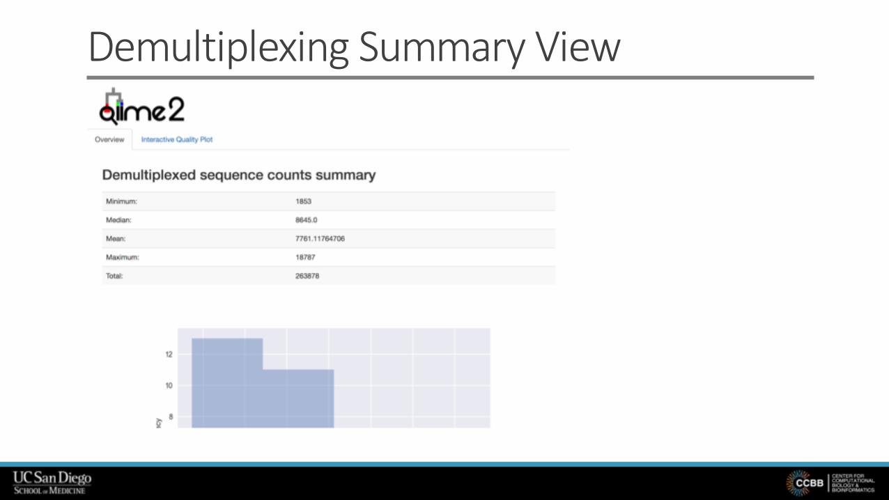
Demultiplexing Summary View

Demultiplexing Summary View (cont.)
Demultiplexing Summary View (cont.)
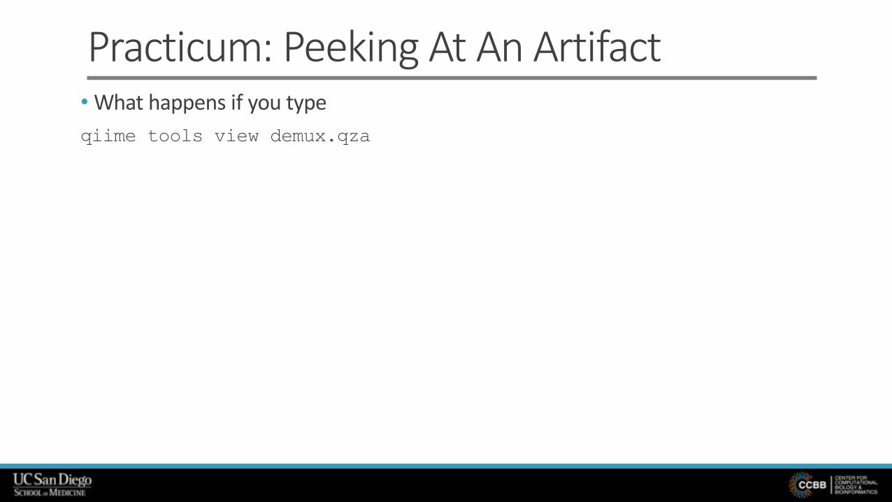
Practicum: Peeking At An Artifact•What happens if you typeqiime tools view demux.qza

Practicum: Peeking At An Artifact (cont.)•What happens if you typeqiime tools view demux.qza
• You getUsage: qiime tools view [OPTIONS] VISUALIZATION_PATH
Error: Invalid value: demux-filtered.qza is not a QIIME 2 Visualization. Only QIIME 2 Visualizations can be viewed
• Instead, runqiime tools view demux.qza
• See something likeUUID: cce55836-0f04-42de-8476-83224254b419Type: SampleData[SequencesWithQuality]Data format: SingleLanePerSampleSingleEndFastqDirFmt

Aside: Viewing Artifact Provenance• Provenance tracking is absolutely critical to reproducible analyses
◦ Almost no tool actually tracks it for you—really a fantastic new QIIME 2 feature
• Provenance can be viewed through the QIIME2 View website◦ Open Chrome and go to https://view.qiime2.org◦ Drag and drop file demux.qza◦ Click on “Provenance” tab
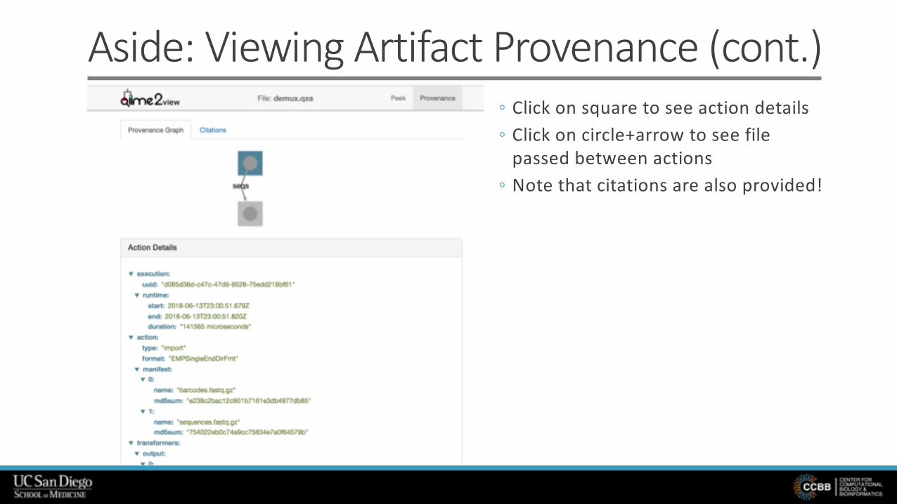
Aside: Viewing Artifact Provenance (cont.)◦ Click on square to see action details◦ Click on circle+arrow to see file
passed between actions◦ Note that citations are also provided!

Quality Control
Bokulich, N. et al. (2013). Quality-filtering vastly improves diversity estim
ates from Illum
inaamplicon
sequencing. Nat M
ethods, 10(1), 57–59.
QIIME defaults:• r = 3 • q = 3• p = 0.75• n = 0• c = 0.005% or 2
Practicum: Quality Controlqiime quality-filter q-score \--i-demux demux.qza \--o-filtered-sequences demux-filtered.qza \--o-filter-stats demux-filter-stats.qza

Practicum: Quality Control (cont.)qiime quality-filter q-score \--i-demux demux.qza \--o-filtered-sequences demux-filtered.qza \--o-filter-stats demux-filter-stats.qza
qiime metadata tabulate \--m-input-file demux-filter-stats.qza \--o-visualization demux-filter-stats.qzv
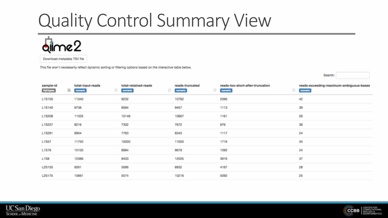
Quality Control Summary View

Practicum: Feature Table Creation
• This can take up to 10 minutes to run, so while we wait …◦ Where do you guess the number 120 came from?
qiime deblur denoise-16S \--i-demultiplexed-seqs demux-filtered.qza \--p-trim-length 120 \--o-representative-sequences rep-seqs.qza \--o-table table.qza \--p-sample-stats \--o-stats deblur-stats.qza

Practicum: Feature Table Creationqiime deblur denoise-16S \--i-demultiplexed-seqs demux-filtered.qza \--p-trim-length 120 \--o-representative-sequences rep-seqs.qza \--o-table table.qza \--p-sample-stats \--o-stats deblur-stats.qza

Feature Table Creation—The Past• Last year: OTU (Operational Taxonomic Unit)
◦ “an operational definition of a species used when only DNA sequence data is available”◦ Sequences at/above a given similarity threshold considered part of the same OTU§ 97% is the usual “species-level” threshold−Similarity determined using alignment (time-consuming)
§ Purpose is to minimize impact of sequencing errors−But also masks fine (sub-OTU) variation in real biological sequences
◦ Results very difficult to compare across studies if done de novo§ “Closed reference”, “open reference” methods increase comparability require reference database
• Output is a “feature table”:§ Rows are samples§ Columns are OTUs (arbitrary identifiers if de novo, from reference database if closed reference)§ Values are frequency of reads from that OTU in that sample
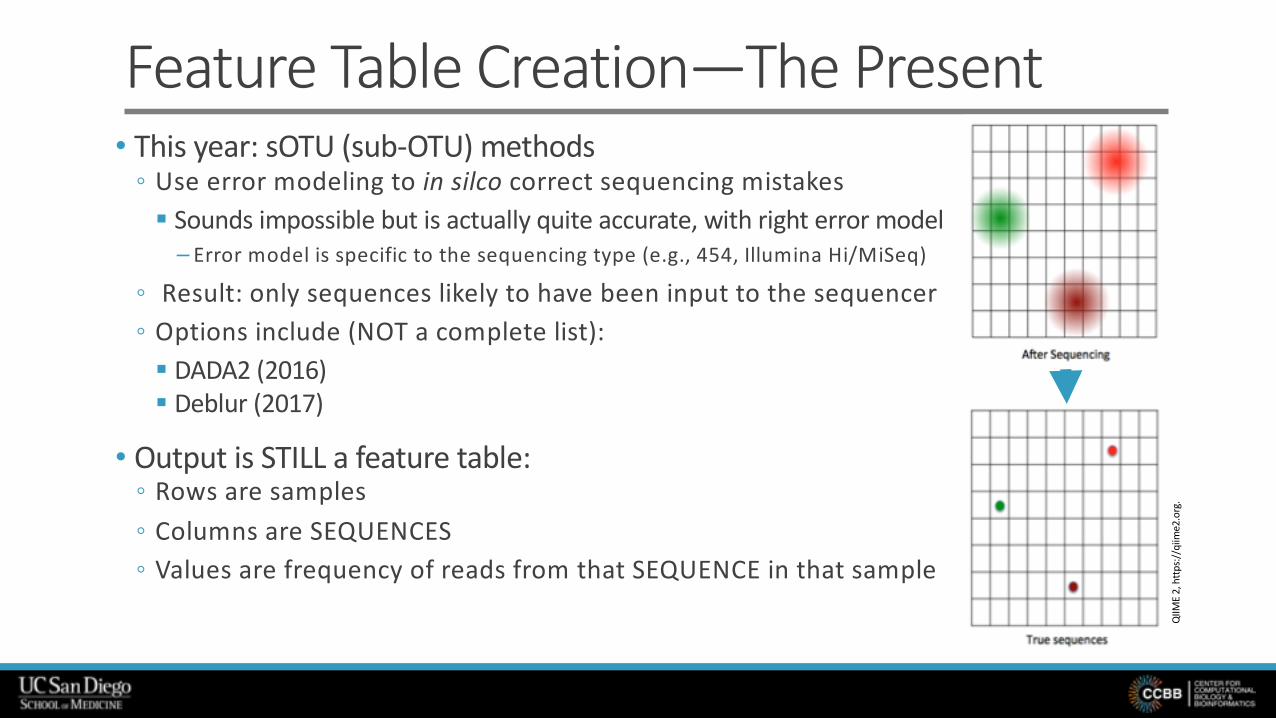
Feature Table Creation—The Present• This year: sOTU (sub-OTU) methods
◦ Use error modeling to in silco correct sequencing mistakes§ Sounds impossible but is actually quite accurate, with right error model−Error model is specific to the sequencing type (e.g., 454, Illumina Hi/MiSeq)
◦ Result: only sequences likely to have been input to the sequencer◦ Options include (NOT a complete list):§ DADA2 (2016)§ Deblur (2017)
• Output is STILL a feature table:◦ Rows are samples◦ Columns are SEQUENCES◦ Values are frequency of reads from that SEQUENCE in that sample
QIIM
E 2,
http
s://q
iime2
.org
.
Practicum: Feature Table Creation (cont.)qiime deblur visualize-stats \--i-deblur-stats deblur-stats.qza \--o-visualization deblur-stats.qzv

Deblur Statistics View

Practicum: Feature Table Creation (cont.)qiime feature-table summarize \--i-table table.qza \--o-visualization table.qzv \--m-sample-metadata-file sample-metadata.tsv
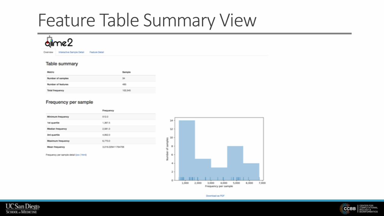
Feature Table Summary View

Feature Table Summary View (cont.)

Feature Table Summary View (cont.)

Feature Table Summary View (cont.)

Feature Table Summary View (cont.)
…
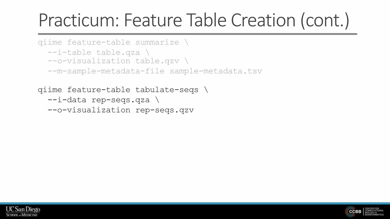
Practicum: Feature Table Creation (cont.)qiime feature-table summarize \--i-table table.qza \--o-visualization table.qzv \--m-sample-metadata-file sample-metadata.tsv
qiime feature-table tabulate-seqs \--i-data rep-seqs.qza \--o-visualization rep-seqs.qzv

Feature Table Tabulation View

Phylogenetic Tree Creation• Evolution is the core concept of biology
◦ There’s only so much you can learn from microbes while ignoring evolution!
• Evolution-aware analyses of a dataset need a phylogenetic tree of its sequences◦ De novo: infer tree using only sequences from dataset◦ Reference-based: insert sequences from dataset into an existing phylogenetic tree§ Not all existing phylogenies are created equal—have strengths and weaknesses based on
intended purpose when developed
• Phylogenetically based analyses in QIIME 2 need a rooted tree
Unrooted: Rooted:
Geer, R.C., Messersmith, D.J, Alpi, K., Bhagwat, M., Chattopadhyay, A., Gaedeke, N., Lyon, J., Minie, M.E., Morris, R.C., Ohles, J.A., Osterbur, D.L. & Tennant, M.R. 2002. NCBI Advanced Workshop for Bioinformatics Information Specialists. [Online] http://www.ncbi.nlm.nih.gov/Class/NAWBIS/.

Practicum: Phylogenetic Tree Creation
• Note: here we are doing de novo phylogenetic tree creation◦ Not necessarily the BEST approach, but an easy one to show you J
qiime alignment mafft \--i-sequences rep-seqs.qza \--o-alignment aligned-rep-seqs.qza

Practicum: Phylogenetic Tree Creation (cont.)qiime alignment mafft \--i-sequences rep-seqs.qza \--o-alignment aligned-rep-seqs.qza
qiime alignment mask \--i-alignment aligned-rep-seqs.qza \--o-masked-alignment masked-aligned-rep-seqs.qza

Practicum: Phylogenetic Tree Creation (cont.)qiime alignment mafft \--i-sequences rep-seqs.qza \--o-alignment aligned-rep-seqs.qza
qiime alignment mask \--i-alignment aligned-rep-seqs.qza \--o-masked-alignment masked-aligned-rep-seqs.qza
qiime phylogeny fasttree \--i-alignment masked-aligned-rep-seqs.qza \--o-tree unrooted-tree.qza
qiime phylogeny midpoint-root \--i-tree unrooted-tree.qza \--o-rooted-tree rooted-tree.qza
• No visualizations provided for these artifacts
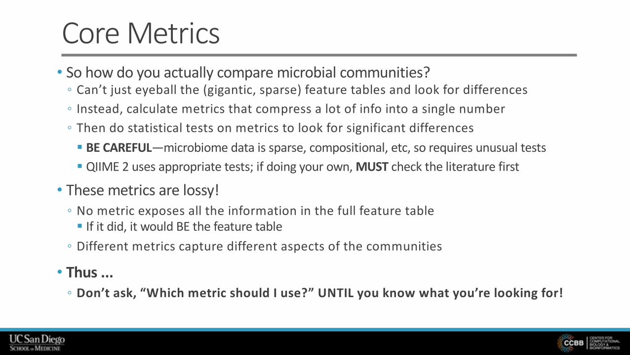
Core Metrics• So how do you actually compare microbial communities?
◦ Can’t just eyeball the (gigantic, sparse) feature tables and look for differences◦ Instead, calculate metrics that compress a lot of info into a single number◦ Then do statistical tests on metrics to look for significant differences§ BE CAREFUL—microbiome data is sparse, compositional, etc, so requires unusual tests§ QIIME 2 uses appropriate tests; if doing your own, MUST check the literature first
• These metrics are lossy!◦ No metric exposes all the information in the full feature table§ If it did, it would BE the feature table
◦ Different metrics capture different aspects of the communities
• Thus ...◦ Don’t ask, “Which metric should I use?” UNTIL you know what you’re looking for!
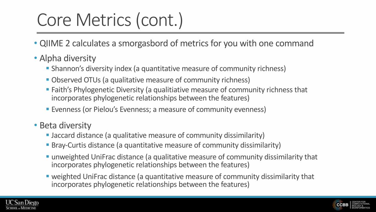
Core Metrics (cont.)• QIIME 2 calculates a smorgasbord of metrics for you with one command• Alpha diversity
§ Shannon’s diversity index (a quantitative measure of community richness)§ Observed OTUs (a qualitative measure of community richness)§ Faith’s Phylogenetic Diversity (a qualitiative measure of community richness that
incorporates phylogenetic relationships between the features)§ Evenness (or Pielou’s Evenness; a measure of community evenness)
• Beta diversity§ Jaccard distance (a qualitative measure of community dissimilarity)§ Bray-Curtis distance (a quantitative measure of community dissimilarity)§ unweighted UniFrac distance (a qualitative measure of community dissimilarity that
incorporates phylogenetic relationships between the features)§ weighted UniFrac distance (a quantitative measure of community dissimilarity that
incorporates phylogenetic relationships between the features)

Normalization for Core Metrics
• Normalization is necessary for valid comparisons of abundance/diversity◦ “But how?!”§ Longstanding approach: rarefaction (reduce all samples to uniform sampling depth)§ Recent publication caused concern− Waste not, want not: why rarefying microbiome data is inadmissible. McMurdie PJ, Holmes S. PLoS
Comput Biol. 2014;10(4).
§ Further work demonstrated concern is excessive− Normalization and microbial differential abundance strategies depend upon data characteristics.
Weiss S, et al. Microbiome. 2017 Mar 3;5(1):27. (Note: I’m an author, so not objective)
• Calculated metric values depend on sampling depth• Ex: circled column has more non-zero counts than others
◦ Is its community really more diverse—or do we just SEE more?◦ Samples with more sequences (greater sampling depth) show
more diversity

Rarefaction• What is rarefaction?
◦ randomly subsampling the same number of sequences from each sample◦ NB: samples without that number of sequences are discarded
• Concerns:◦ Too low: ignore a lot of samples’ information
◦ Too high: ignore a lot of samples
◦ Still a good choice for normalization (Weiss S, et al. Microbiome. 2017):§ “Rarefying more clearly clusters samples according to biological origin than other
normalization techniques do for ordination metrics based on presence or absence”§ “Alternate normalization measures are potentially vulnerable to artifacts due to library
size”
• Researcher must choose sampling depth—but how?

Sampling Depth Selection• Don’t sweat it too much
◦ “Low” depths (10-1000 sequences per sample) capture all but very subtle variations
◦ Retaining samples is usually more important than retaining sequences§ May care not just how many samples are left out but WHICH samples are left out
Fig. 2 , Kuczynski, J. et al., "D irect sequencing of the hum an m icrobiom e readily reveals com m unity d ifferences", G enom e B io logy, 2010

Practicum: Core Metricsqiime diversity core-metrics-phylogenetic \--i-phylogeny rooted-tree.qza \--i-table table.qza \--p-sampling-depth ??? \--m-metadata-file sample-metadata.tsv--output-dir metrics
•Which sampling depth should we use?◦ How can we decide?

Exercise: Core Metricsqiime diversity core-metrics-phylogenetic \--i-phylogeny rooted-tree.qza \--i-table table.qza \--p-sampling-depth ??? \--m-metadata-file sample-metadata.tsv--output-dir metrics
•Which sampling depth should we use?◦ How can we decide?
◦ Work with your partner to choose a sampling depth, then answer:§ Why did you choose this value?§ How many samples will be excluded from your analysis based on this choice?§ How many total sequences will you be analyzing in the core metrics command?
qiime tools view table.qzv

Answers: Core Metricsqiime diversity core-metrics-phylogenetic \--i-phylogeny rooted-tree.qza \--i-table table.qza \--p-sampling-depth 800 \--m-metadata-file sample-metadata.tsv--output-dir metrics
•My answers:◦ Why did you choose this value?§ Anything higher excludes >= half of right palm samples
◦ How many samples will be excluded from your analysis based on this choice?§ 4, all from right palm of subject 1
◦ How many total sequences will you be analyzing in the core metrics command?§ 24,000 (23.40%)
• Note: there is no single visualization for core metrics
Alpha Diversity• “Within-sample” diversity
◦ Many different metrics exist § Taxonomy-based (e.g., number of observed OTUs)−Assume everything is equally dissimilar−More likely to see differences based on close relatives
§ Phylogeny-based (e.g., phylogenetic diversity over whole tree)−Treat less related items as more dissimilar−Better at scaling the observed differences
◦ The “correct” metric(s) are those relevant to your hypothesis§ Please do HAVE a hypothesis!
• Testing approach:◦ Examine alpha diversity metric by metadata values◦ Test whether differences in metric distribution is different between groups (if
metadata is categorical) or correlated with metadata (if metadata is continuous)

Number of OTUs by sampling site
Alpha Diversity

Number of OTUs by sampling site
Alpha Diversity
High within-sample diversity—why?
Practicum: Alpha Diversity Group Significance
• Note: only showing you the group significance visualization of ONE alpha diversity metric◦ Remember that 3 others are calculated by core-metrics-phylogenetic alone◦ The one I am showing is not “the correct one”—pick the one that fits your hypothesis
• To check the group significance of a different metric, just input a different vector file ◦ To find them:
qiime diversity alpha-group-significance \--i-alpha-diversity metrics/faith_pd_vector.qza \--m-metadata-file sample-metadata.tsv \--o-visualization metrics/faith-pd-group-significance.qzv
cd metrics/ls *_vector.qza

Alpha Diversity Group Significance View

Alpha Diversity Group Significance View

Exercise: Alpha Diversity Group Significance
•Work with your partner to answer these questions:◦ Is BodySite value associated with significant differences in phylogenetic diversity?◦ Which two sites have the most significant difference in phylogenetic diversity
distributions?§ Note different between p-value and q-value
◦ Is Subject value associated with significant differences in phylogenetic diversity?
qiime diversity alpha-group-significance \--i-alpha-diversity metrics/faith_pd_vector.qza \--m-metadata-file sample-metadata.tsv \--o-visualization metrics/faith-pd-group-significance.qzv
Answers: Alpha Diversity Group Significance
•My answers:◦ Is BodySite value associated with significant differences in phylogenetic diversity?§ Yes, with p < 1 E-3
◦ Which two sites have the most significantly difference in phylogenetic diversity distributions?§ Left palm is (equally) most significantly different from gut and tongue−Consider: any idea why perhaps left palm but not right?
◦ Is Subject value associated with significant differences in phylogenetic diversity?§ No
qiime diversity alpha-group-significance \--i-alpha-diversity metrics/faith_pd_vector.qza \--m-metadata-file sample-metadata.tsv \--o-visualization metrics/faith-pd-group-significance.qzv
Practicum: Alpha Diversity Correlation
• Same caveat as before: ◦ Only showing the correlation visualization of ONE alpha diversity metric§ Not necessarily “the correct one”!
qiime diversity alpha-correlation \--i-alpha-diversity metrics/evenness_vector.qza \--m-metadata-file sample-metadata.tsv \--o-visualization metrics/evenness-alpha-correlation.qzv

Alpha Diversity Correlation View

Beta Diversity• “Between-sample” diversity
◦ Has similar categories, caveats as ! diversity
• A popular phylogenetic option is 'UniFrac’: ◦ Measures how different two samples' component sequences are
◦ Weighted UniFrac: takes abundance each sequence into account
Illus
trat
ion
cour
tesy
of D
r. R
ob K
nigh
t

Beta Diversity Ordination• Ordination: multivariate techniques that arrange samples along axes on the
basis of composition• Principal Coordinates Analysis: a way to map non-Euclidean distances into a
Euclidean space to enable further investigation◦ Abbreviated as PCoA, not to be confused with PCA (Principal Component Analysis)◦ Starting point is distance matrix§ NOT the full set of independent variables for each sample
◦ n pairwise distances are projected into n-1 dimensions◦ PCA performed to reduce the dimensionality back down
• PCoA axes can’t be decomposed into independent variable contributions◦ But results can be compared to metadata to identify patterns
A B C
A BC
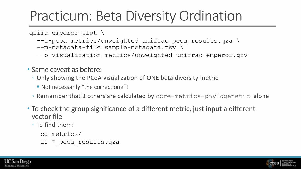
Practicum: Beta Diversity Ordinationqiime emperor plot \--i-pcoa metrics/unweighted_unifrac_pcoa_results.qza \--m-metadata-file sample-metadata.tsv \--o-visualization metrics/unweighted-unifrac-emperor.qzv
• Same caveat as before: ◦ Only showing the PCoA visualization of ONE beta diversity metric
§ Not necessarily “the correct one”!
◦ Remember that 3 others are calculated by core-metrics-phylogenetic alone
• To check the group significance of a different metric, just input a different vector file ◦ To find them:
cd metrics/ls *_pcoa_results.qza

Beta Diversity Ordination View

Exercise: Beta Diversity Ordination
•Work with your partner to answer the following question:◦ Can you find a metadata category that appears associated with the observed clusters? § Hint: Experiment with coloring points by different metadata
qiime emperor plot \--i-pcoa metrics/unweighted_unifrac_pcoa_results.qza \--m-metadata-file sample-metadata.tsv \--o-visualization metrics/unweighted-unifrac-emperor.qzv

Answers: Beta Diversity Ordination
•My answer:◦ Can you find a metadata category that appears associated with the observed clusters? § Yep: BodySite
qiime emperor plot \--i-pcoa metrics/unweighted_unifrac_pcoa_results.qza \--m-metadata-file sample-metadata.tsv \--o-visualization metrics/unweighted-unifrac-emperor.qzv
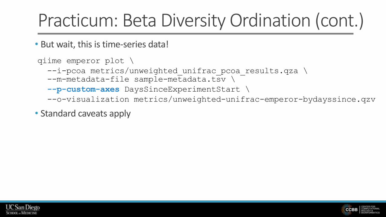
Practicum: Beta Diversity Ordination (cont.)• But wait, this is time-series data!qiime emperor plot \--i-pcoa metrics/unweighted_unifrac_pcoa_results.qza \--m-metadata-file sample-metadata.tsv \--p-custom-axes DaysSinceExperimentStart \--o-visualization metrics/unweighted-unifrac-emperor-bydayssince.qzv
• Standard caveats apply

Beta Diversity Ordination View (cont.)

Practicum: Beta Diversity Group Significance
• Standard caveats apply
qiime diversity beta-group-significance \--i-distance-matrix metrics/unweighted_unifrac_distance_matrix.qza \--m-metadata-file sample-metadata.tsv \--m-metadata-column BodySite \--p-pairwise \--o-visualization metrics/unweighted-unifrac-bodysite-significance.qzv

Beta Diversity Group Significance View
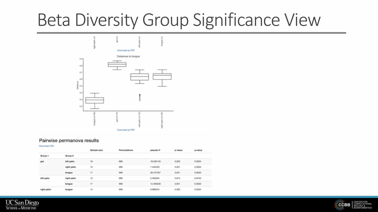
Beta Diversity Group Significance View

Exercise: Beta Diversity Group Significance
•Work with your partner to answer these questions:◦ Does the group significance analysis bear out your intuition from the ordination?§ If so, are the differences statistically significant?§ Are there specific pairs of BodySite values that are significantly different from each other?
◦ How about Subject?§ Hint: you will need to run a new command!
qiime diversity beta-group-significance \--i-distance-matrix metrics/unweighted_unifrac_distance_matrix.qza \--m-metadata-file sample-metadata.tsv \--m-metadata-category BodySite \--p-pairwise \--o-visualization metrics/unweighted-unifrac-bodysite-significance.qzv

Answers: Beta Diversity Group Significance
•My answers:◦ Does the group significance analysis bear out your intuition from the ordination?§ Yes§ If so, are the differences statistically significant?−Yes, with p <= 0.001 (bonus: why do I say ”less than or equal to”?)
§ Are there specific pairs of BodySite values that are significantly different from each other?−Yes, all of the pairs except left palm/right palm
qiime diversity beta-group-significance \--i-distance-matrix metrics/unweighted_unifrac_distance_matrix.qza \--m-metadata-file sample-metadata.tsv \--m-metadata-category BodySite \--p-pairwise \--o-visualization metrics/unweighted-unifrac-bodysite-significance.qzv
Taxonomic Assignment• Sequence features or OTUs have limited utility
◦ At some point, you’ll want to link your findings to published work
◦ That requires identifying the taxonomy of each sequence feature
• Steps:◦ Pick reference database§ I hear you cry, “Which one should I use?”
◦ Train a classifier algorithm to assign taxonomies to sequences
§ Use the reference database as the training set
◦ Run the classifier algorithm on your sequence features

Taxonomic Assignment• Sequence features or OTUs have limited utility
◦ At some point, you’ll want to link your findings to published work◦ That requires identifying the taxonomy of each sequence feature
• Steps:◦ Pick reference database§ I hear you cry, “Which one should I use?”
◦ Train a classifier algorithm to assign taxonomies to sequences§ Use the reference database as the training set
◦ Run the classifier algorithm on your sequence features

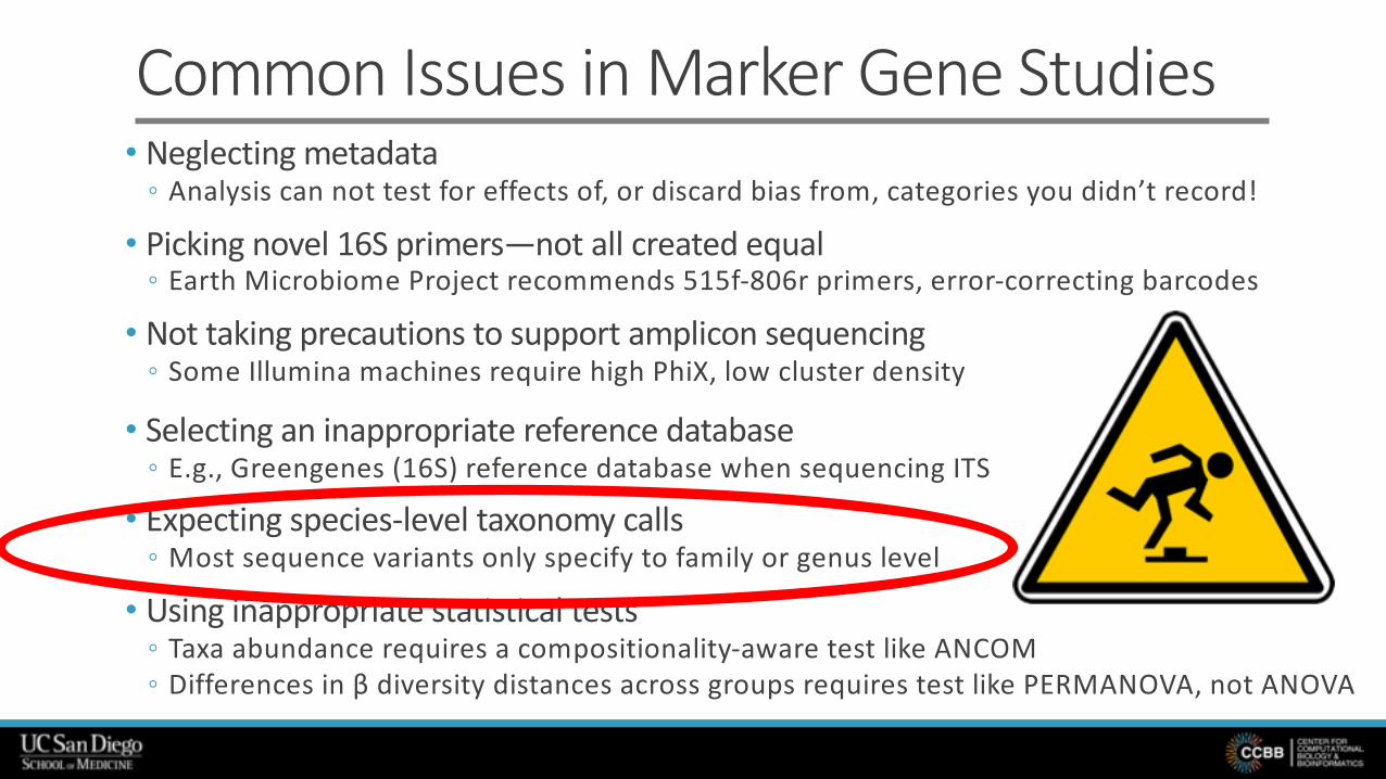
Common Issues in Marker Gene Studies• Neglecting metadata
◦ Analysis can not test for effects of, or discard bias from, categories you didn’t record!
• Picking novel 16S primers—not all created equal◦ Earth Microbiome Project recommends 515f-806r primers, error-correcting barcodes
• Not taking precautions to support amplicon sequencing◦ Some Illumina machines require high PhiX, low cluster density
• Selecting an inappropriate reference database◦ E.g., Greengenes (16S) reference database when sequencing ITS
• Expecting species-level taxonomy calls◦ Most O sequence variants only specify to family or genus level
• Using inappropriate statistical tests◦ Taxa abundance requires a compositionality-aware test like ANCOM◦ Differences in β diversity distances across groups requires test like PERMANOVA, not ANOVA
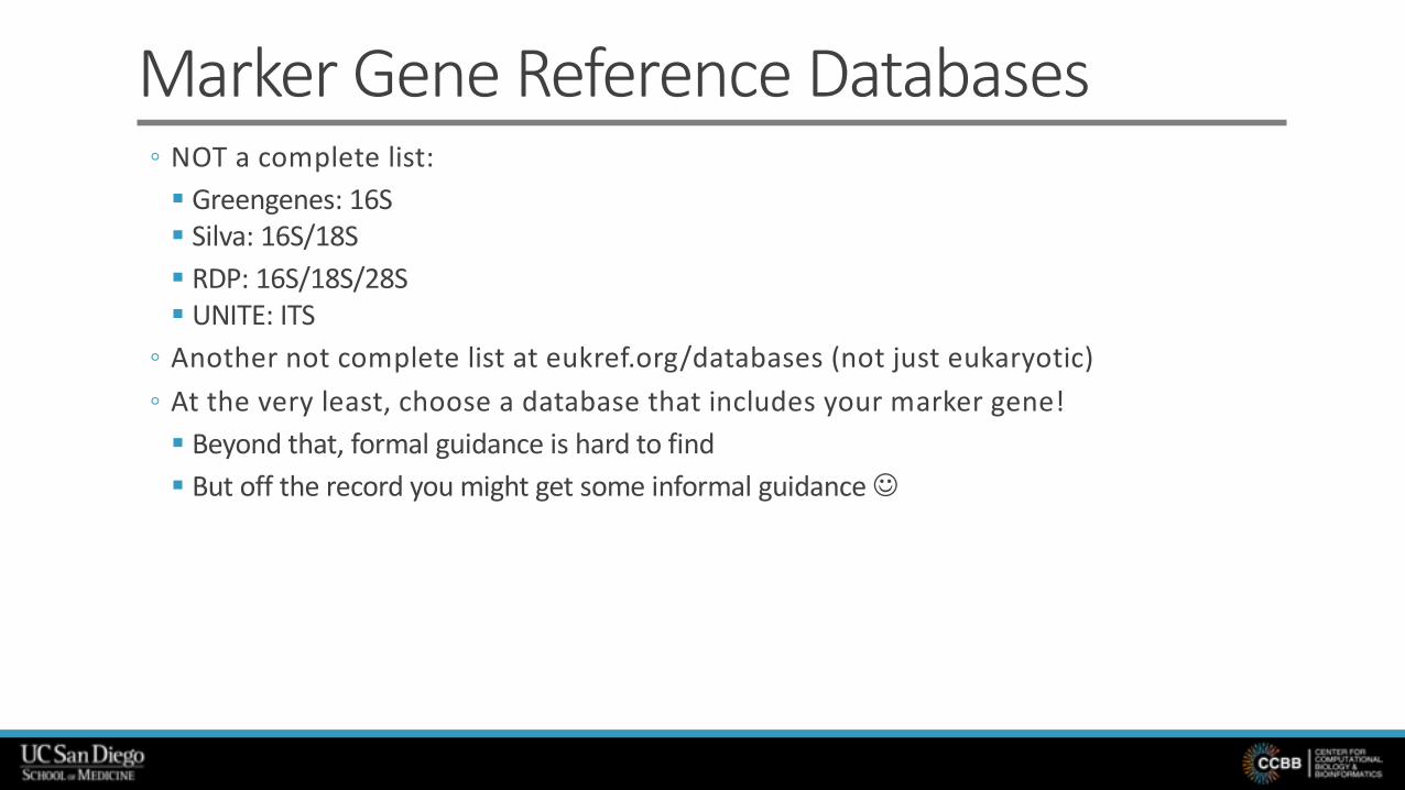
Marker Gene Reference Databases◦ NOT a complete list:§ Greengenes: 16S§ Silva: 16S/18S§ RDP: 16S/18S/28S§ UNITE: ITS
◦ Another not complete list at eukref.org/databases (not just eukaryotic)◦ At the very least, choose a database that includes your marker gene!§ Beyond that, formal guidance is hard to find§ But off the record you might get some informal guidance J

Taxonomic Assignment• Sequence features or OTUs have limited utility
◦ At some point, you’ll want to link your findings to published work
◦ That requires identifying the taxonomy of each sequence feature
• Steps:◦ Pick reference database§ I hear you cry, “Which one should I use?”
◦ Train a classifier algorithm to assign taxonomies to sequences
§ Use the reference database as the training set
◦ Run the classifier algorithm on your sequence features
Common Issues in Marker Gene Studies• Neglecting metadata
◦ Analysis can not test for effects of, or discard bias from, categories you didn’t record!
• Picking novel 16S primers—not all created equal◦ Earth Microbiome Project recommends 515f-806r primers, error-correcting barcodes
• Not taking precautions to support amplicon sequencing◦ Some Illumina machines require high PhiX, low cluster density
• Selecting an inappropriate reference database◦ E.g., Greengenes (16S) reference database when sequencing ITS
• Expecting species-level taxonomy calls◦ Most sequence variants only specify to family or genus level
• Using inappropriate statistical tests◦ Taxa abundance requires a compositionality-aware test like ANCOM◦ Differences in β diversity distances across groups requires test like PERMANOVA, not ANOVA

Taxonomy: Expectation Vs RealityIdeal Result Real Result
Kingdom Bacteria BacteriaPhylum Proteobacteria ProteobacteriaClass Gammaproteobacteria GammaproteobacteriaOrder Enterobacteriales EnterobacterialesFamily Enterobacteriaceae EnterobacteriaceaeGenus Eschericia ---Species coli OTU 2445338Strain O157:H7 --

Practicum: Taxonomic Assignment
• Note: the classifier has already been trained for you
◦ trained on the Greengenes 13_8 99% OTUs
◦ sequences trimmed to only include 250 bases from the region of the 16S that was
sequenced in this analysis
§ the V4 region, bound by the 515F/806R primer pair
• Other pre-trained classifiers available in Data Resources page on docs.qiime2.org
qiime feature-classifier classify-sklearn \--i-classifier gg-13-8-99-515-806-nb-classifier.qza \--i-reads rep-seqs.qza \--o-classification taxonomy.qza

Practicum: Taxonomic Assignmentqiime feature-classifier classify-sklearn \--i-classifier gg-13-8-99-515-806-nb-classifier.qza \--i-reads rep-seqs.qza \--o-classification taxonomy.qza
qiime metadata tabulate \--m-input-file taxonomy.qza \--o-visualization taxonomy.qzv

Taxonomic Assignment Tabulation View
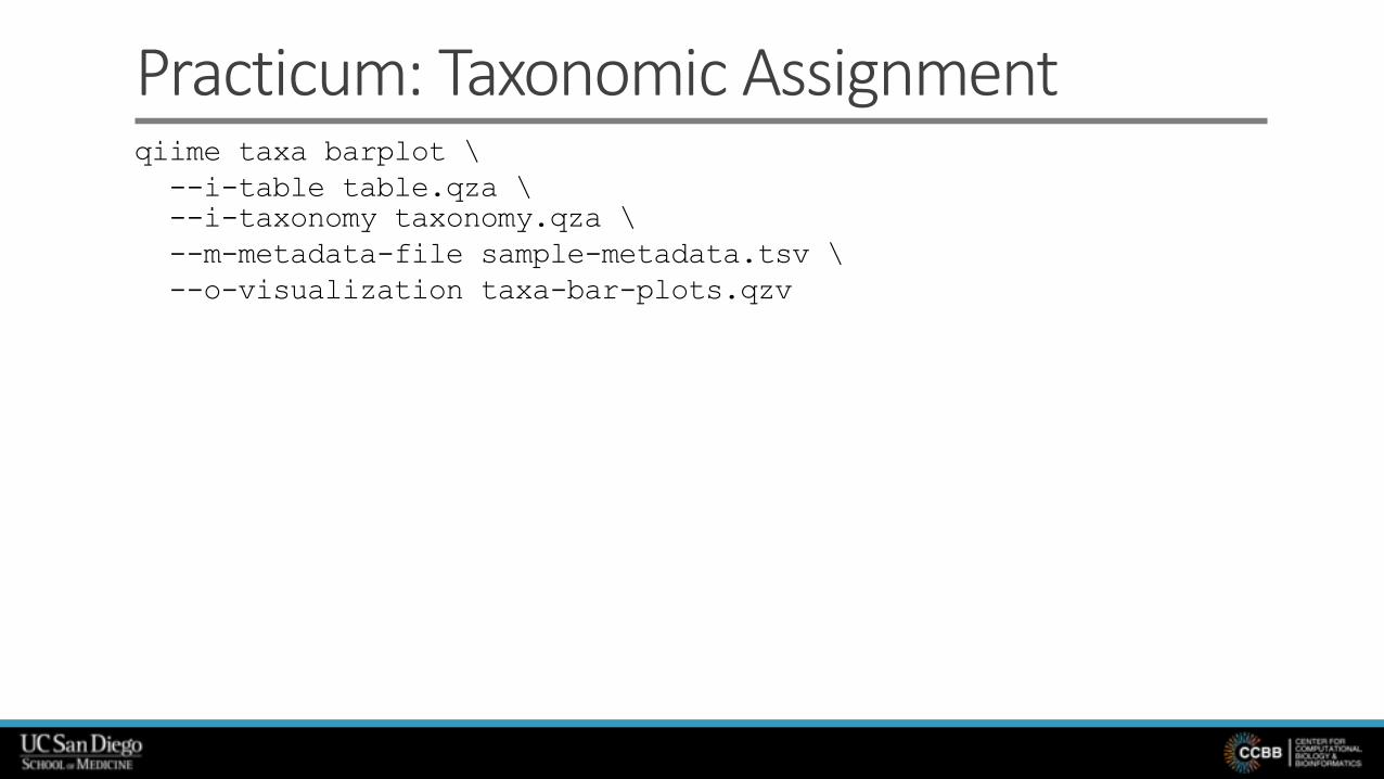
Practicum: Taxonomic Assignmentqiime taxa barplot \--i-table table.qza \--i-taxonomy taxonomy.qza \--m-metadata-file sample-metadata.tsv \--o-visualization taxa-bar-plots.qzv

Taxonomic Assignment Bar Plot View

Exercise: Taxonomic Assignment
• “Level 1” = kingdom, “Level 2” = phylum, etc•Work with your partner to:
◦ Visualize the taxa at level 2◦ Sort the samples by BodySite◦ Do you see anything suggestive?
qiime taxa barplot \--i-table table.qza \--i-taxonomy taxonomy.qza \--m-metadata-file sample-metadata.tsv \--o-visualization taxa-bar-plots.qzv

Answers: Taxonomic Assignment
• Gut sure seems to have a lot more Bacteroidetesthan the other sites

Differential Abundance Analysis•Why go to the trouble of assigning taxonomies?
◦ Probably you want to know whether any particular taxa are differentially abundant§ In different individuals, environments, time points, etc
• How to test for differential abundance?◦ Microbiome datasets are “compositional” (fixed sum)
Taxon 1Taxon 2Taxon 3Taxon 4
Group 1 Reads
Taxon 1Taxon 2Taxon 3Taxon 4
Group 2 Reads

Differential Abundance Analysis•Why go to the trouble of assigning taxonomies?
◦ Probably you want to know whether any particular taxa are differentially abundant§ In different individuals, environments, time points, etc
• How to test for differential abundance?◦ Microbiome datasets are “compositional” (fixed sum)
◦ Watch out: “traditional” statistical methods perform badly for this sort of data§ e.g., t-test, ANOVA§ False discovery rate can be as high as 90%!
Taxon 1Taxon 2Taxon 3Taxon 4
Group 1 Reads
Taxon 1Taxon 2Taxon 3Taxon 4
Group 2 Reads Fo
ld-c
hang
e 2
-2
Group 2 vs Group 1

Differential Abundance Analysis (cont.)◦ What to use instead?
§ ANCOM (Analysis of Composition of Microbiomes)
−Identifies taxa that are present in different abundances across sample groups
◦ Compares log ratio of the abundance of each taxon to abundance of all remaining taxa one at a time
−Assumes that <25% of the features are changing between groups—not a given!
§ ilr (Isometric Log Ratio transforms—a.k.a. balance trees or gneiss)
−Identifies microbial subcommunities that present in different abundances across sample groups
§ Neither require rarefication of inputs
§ Both recommend filtering out taxa that don’t contain much info, such as
−Features that have few reads (i.e. less than 10 reads across all samples).
−Features that are rarely observed (i.e. present in less than 5 samples in a study).
−Features that have very low variance (i.e. less than 10e-4)
◦ This is left as an exercise for the reader J Check out feature-table filter-samples

Practicum: ANCOM Analysis•We already saw in that different body sites look very different• Given that, probably many features (sequences) are changing in abundance
across body sites◦ This violates ANCOM’s statistical assumption!
• Therefore, limit ANCOM analysis to samples from a single body site:qiime feature-table filter-samples \--i-table table.qza \--m-metadata-file sample-metadata.tsv \--p-where "BodySite='gut'" \--o-filtered-table gut-table.qza
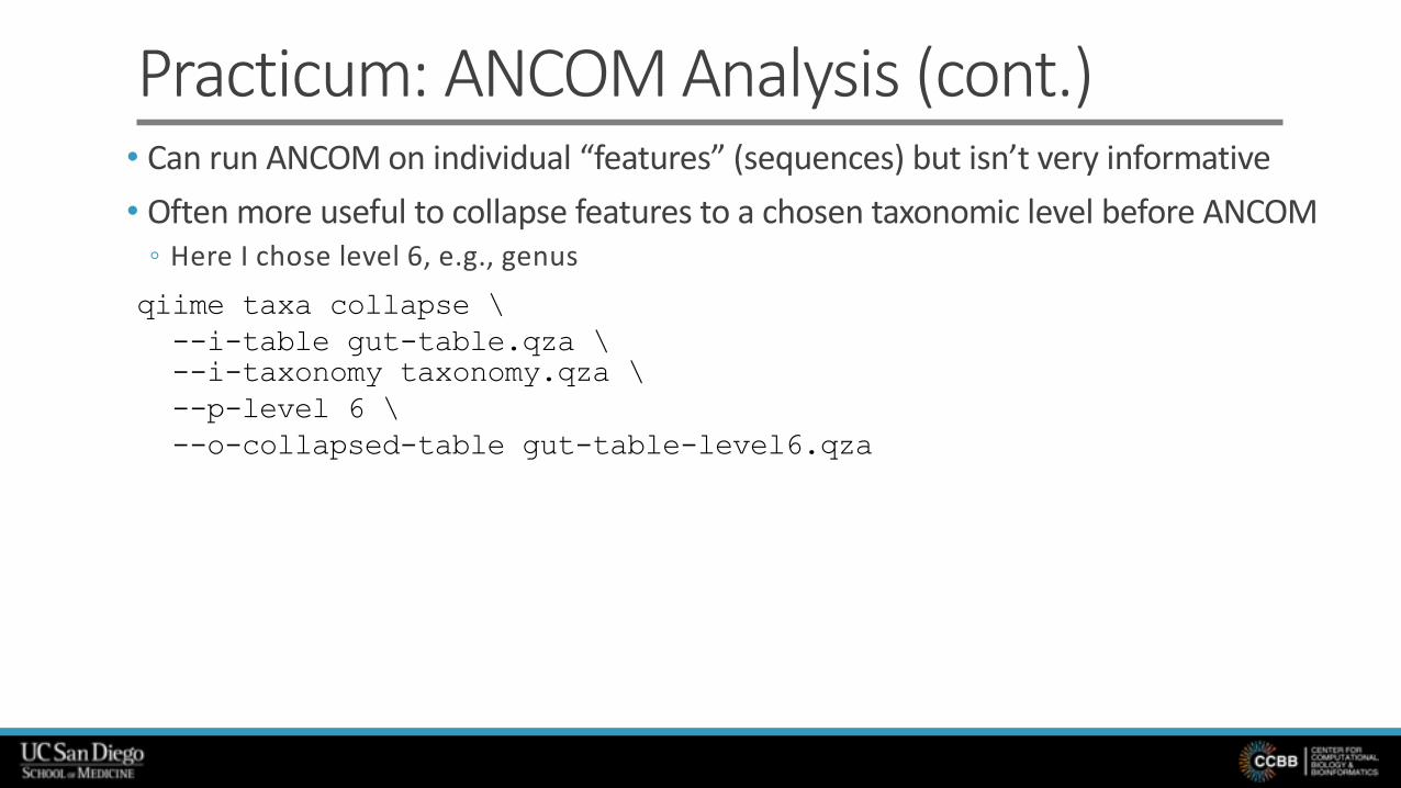
Practicum: ANCOM Analysis (cont.)• Can run ANCOM on individual “features” (sequences) but isn’t very informative• Often more useful to collapse features to a chosen taxonomic level before ANCOM
◦ Here I chose level 6, e.g., genusqiime taxa collapse \--i-table gut-table.qza \--i-taxonomy taxonomy.qza \--p-level 6 \--o-collapsed-table gut-table-level6.qza

Practicum: ANCOM Analysis (cont.)• Internally, ANCOM takes logs—and log of zero is undefined
◦ Common approach: add one count to every value (pseudocount)◦ Not limited to ANCOM—used for any log-based method
qiime composition add-pseudocount \--i-table gut-table-level6.qza \--o-composition-table comp-gut-table-level6.qza

Practicum: ANCOM Analysis (cont.)qiime composition ancom \--i-table comp-gut-table-level6.qza \--m-metadata-file sample-metadata.tsv \--m-metadata-column Subject \--o-visualization ancom-subject-level6.qzv

ANCOM View

Details: ANCOM View•W-statistic
◦ # of features that a single feature is tested to be significantly different against◦ ANCOM internally decides what W value indicates significance, returns only
significant results§ You aren’t going to find a p-value here, no matter how hard you look J
• Percentile abundance table:◦ A table of features and their percentile abundances in each group◦ Rows are features or taxa◦ Columns are percentile within a group◦ Values are abundance of reads for given percentile for that group § e.g.: The lowest-in-this-taxon 25% of samples in ”group” subject-2 had 100.75 or fewer
sequences assigned to this taxon

ilr and Balance Trees•Microbiome sequence data give proportions of taxa abundance◦ Because of compositionality
• “[B]ased on proportions alone, it is impossible to determine whether the growth or decline of any individual species has truly occurred”• Balance trees instead ask an
answerable question:◦ Has the balance of sub-
communities changed?
Quote and figure from Morton et al, mSystems 2017
Sample 1 Sample 2

ilr and Balance Trees (cont.)
• The subcommunities of interest are defined by a tree of all the species◦ Each internal node in the tree is a “balance” between the subcommunities in its left
and right children
• For each sample, at each balance, calculate the isometric log ratio transform (ilr)◦ Gives a measure of relative abundance of subcommunities on each side of the balance
Sample 1 Sample 2=0.36
=-0 .21
=-0 .08
=0.34
=0.26
=-0 .21
=0.33
=0
Fig
mod
ified
from
Mor
ton
et a
l, m
Syst
ems2
017

ilr and Balance Trees (cont.)• After ilr, result is a matrix
◦ ilr values by sample by balance
• Simple case:◦ Only one balance is of interest◦ Can just do Student’s t-test
•More realistic case:◦ All balances are of interest§ Want to characterize whole community
◦ Do multivariate response linear regression§ Fit a linear regression model for each balance
based on all samples for that balance−e.g., Yb1 = β1X1 + β2X2+ β3X3 + …. βiXi + εb1
§ Coefficients significantly ≠ 0 = categories associated w/difference in subcommunities of balance
b1 b2 b3 b4
Sample 1 0.36 -0.08 -0.21 0.34
Sample 2 0.26 0.33 -0.21 0.00
b1 b2 b3 b4
Sample 1 0.36 -0.08 -0.21 0.34
Sample 3 0.33 -0.11 -0.20 0.29
Sample 5 0.37 -0.03 -0.18 0.35
Sample 2 0.26 0.33 -0.21 0.00
Sample 4 0.28 0.30 -0.22 0.01
Sample 6 0.25 0.34 -0.20 0.02
Gro
up 1
Gro
up 2

Practicum: gneiss Analysis• Balance trees were first developed in geology
◦ “gneiss” (say: nice) is a kind of rock
• Like ANCOM, gneiss uses logs, so requires a pseudocountqiime gneiss add-pseudocount \--i-table table.qza \--p-pseudocount 1 \--o-composition-table composition.qza

Practicum: gneiss Analysis (cont.)• The tree used defines which balances are assessed
◦ i.e., which subcommunities of species are compared◦ How to choose it?
• Use an externally defined tree (e.g., phylogeny)
• Build a tree based on a numeric metric related to your hypothesis◦ e.g., from your metadata, such as pH◦ Using gradient clustering gneiss command
• Build a tree with unsupervised clustering across all your data◦ Group together organisms based on how often they co-occur with each other
qiime gneiss correlation-clustering \--i-table composition.qza \--o-clustering hierarchy.qza

Practicum: gneiss Analysis (cont.)•What does the tree actually look like?qiime gneiss dendrogram-heatmap \--i-table composition.qza \--i-tree hierarchy.qza \--m-metadata-file sample-metadata.tsv \--m-metadata-column BodySite \--p-color-map seismic \--o-visualization tree_heatmap_by_bodysite.qzv

gneiss Tree View

Practicum: gneiss Analysis (cont.)• Calculate the ilr transformsqiime gneiss ilr-transform \--i-table composition.qza \--i-tree hierarchy.qza \--o-balances balances.qza
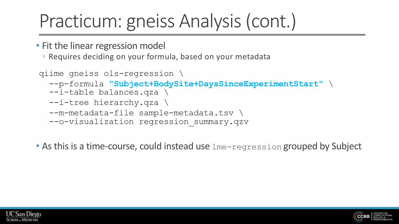
Practicum: gneiss Analysis (cont.)• Fit the linear regression model
◦ Requires deciding on your formula, based on your metadata
• As this is a time-course, could instead use lme-regression grouped by Subject
qiime gneiss ols-regression \--p-formula "Subject+BodySite+DaysSinceExperimentStart" \--i-table balances.qza \--i-tree hierarchy.qza \--m-metadata-file sample-metadata.tsv \--o-visualization regression_summary.qzv
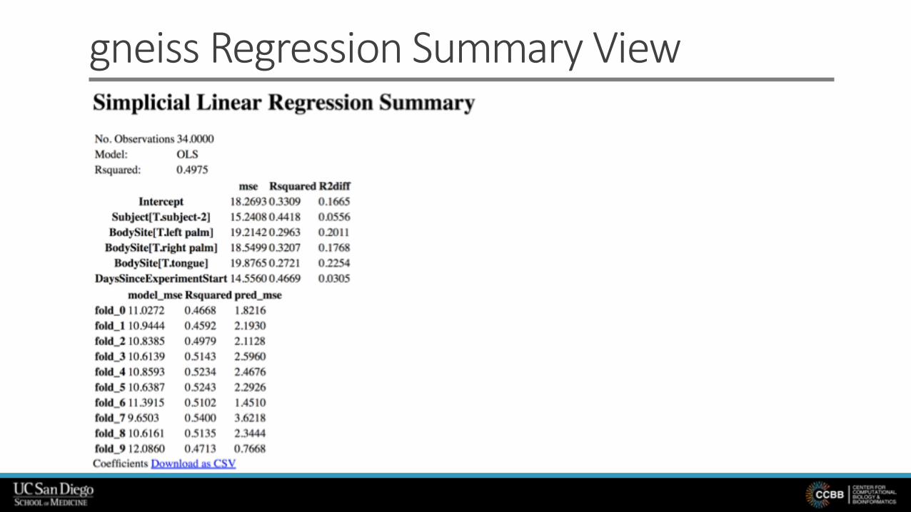
gneiss Regression Summary View

gneiss Regression Summary View (cont.)

gneiss Regression Summary View (cont.)

Practicum: gneiss Analysis (cont.)•Well, great, but we seem to have strayed a long way from actual taxa!qiime gneiss balance-taxonomy \--i-table composition.qza \--i-tree hierarchy.qza \--i-taxonomy taxonomy.qza \--p-taxa-level 2 \--p-balance-name 'y0' \--m-metadata-file sample-metadata.tsv \--m-metadata-column BodySite \--o-visualization y0_taxa_summary.qzv

gneiss Balance Taxa Summary View

gneiss Balance Taxa Summary View• Possible meanings
◦ The taxa in the y0 numerator on average increase in other sites compared to gut
◦ The taxa in the y0 denominator on average decrease in other sites compared to gut
◦ A combination of the above occurs◦ Taxa abundances in both y0 numerator and
y0 denominator both increase compared to gut, but taxa abundances in numerator increase more compared to denominator
◦ Taxa abundances in both y0 numerator and y0 denominator both decrease, but taxa abundances in denominator increase more compared to numerator

gneiss Balance Taxa Summary View (cont.)

Practicum Summary• Steps practiced
◦ Importing data◦ Demultiplexing◦ Running Quality Control◦ Creating a feature table◦ Building a phylogenetic tree◦ Calculating core diversity metrics◦ Testing alpha diversity group significance and correlation◦ Performing beta diversity ordination◦ Testing beta diversity group significance◦ Assigning taxonomies◦ Performing differential abundance analysis with ANCOM and/or gneiss

Acknowledgements• Center for Computational Biology & Bioinformatics, University of California at
San Diego• Caporaso lab, Northern Arizona University
• Knight lab, UCSD• QIIME 2 development team!