MICRO WATERSHED LEVEL WATER RESOURCE MANAGEMENT BASED ON THREE YEARS RUNOFF

ESTIMATION USING REMOTE SENSING AND GIS TECHNIQUES FOR SIMLAPAL BLOCK, BANKURA, W.B

V.S.S.KIRAN

Lead Faculty - IIC Academy, IIC Technologies Ltd, Visakhapatnam, Andhra Pradesh-530041 Email: Kiran.vuppala@iictechnologies.com, Mobile- +91-9474897114

Abstract: Water is one of the essential natural resource, without which life cannot exist. Demand of water is increasing with the increase of population. We need water for agriculture, industry, human and cattle consumption. Therefore it is very important to manage this very essential resource with sustainable manner. Hence, we need proper management and development planning to restore or recharge water where runoff is very high due to various topographical conditions. The Runoff estimation method is one of the significant RSGIS tool for prioritization of micro watershed. Soil Conservation Service Runoff Curve Number is a quantitative descriptor of the land use/land cover, soil complex characteristics of watershed and its computed direct runoff through an empirical relation that requires the rainfall and watershed co-efficient namely runoff curve number. The SCS Curve Number approach to runoff volume is typically thought of as a method for generating storm runoff for rare events and not for water quality design. The parameters were obtained with the help of Erdas, Arc GIS and MS Office. The methodology adapted from SCS method for the seasonal runoff estimation for each micro-watershed is how much prioritized. Using last three years rainfall data and estimate three years runoff than compare the three years priority level and prepared by final priority map. The results revealed that the micro watershed priorities are shows five categorizes very high, high, medium, low and very low priority.

Keywords: Remote Sensing, GIS, Algorithms, Arc GIS, Erdas, Ms Office

1. Introduction:

A watershed is an ideal unit for management of natural resources that also supports land and water resource management for mitigation of the impact of natural disasters for achieving sustainable development. The significant factor for the planning and development of a watershed are its physiographic, drainage, geomorphology, soil, land use/land cover and available water resources. Remote Sensing and GIS are the most proven tools for watershed development, management and also the studies on prioritization of micro-watersheds development and management. Runoff method could be used for prioritization of micro-watersheds by studying hydrological soil group condtions and seasonal rainfall parameters of the watershed with the help of soil and land use/ land cover maps. Water is one of the essential natural resource, without which life cannot exist. Demand of water is increasing with the increase of population. We need

water for agriculture, industry, human and cattle consumption. Therefore it is very important to manage this very essential resource with sustainable manner. Hence, we need proper management and development planning to restore or recharge water where runoff is very high due to various topographical conditions. If proper management is planned that will not only control surface soil erosion but also recharge ground water. Remote Sensing and GIS have become proven tools for the management and development of water resources. Several studies have been carried out worldwide and they have shown excellent results. Due to advancement in satellites and sensing technology, it is possible to map finer details of the earth surface and provide scope for micro level planning and management. The study area that is taken has severe water crises during the summer season. The terrain is highly undulating with very high runoff which causes minimum recharge of ground water in spite of 1750 mm average annual rainfall. This high runoff also causes the erosion of very fertile soil.

The present study aims at water resource management for the prioritization of micro watershed based on three different years runoff estimation using Remote sensing data and GIS overlaying techniques. This study is mainly helpful for the increasing agricultural based livelihood and also to supplying the greater level of irrigation facilities.

1.1. Study Area: The study area has been taken is a part of Silai River Basin in Simlapal block of Bankura district part of West Bengal State. It is located on 22˚59’38.84”North to 22˚50’34.42”North latitude and 86˚55’20.15” to 87˚13’06.10” East longitudes. It has an average elevation of 57mtr (187 feet’s). Simlapal is a community development block is in Khatra subdivision of Bankura district in West Bengal state, and it is bounded by the Khatra block in west, Taldangra block in north, Sarenga block is south and also covered west Midnapur district in east. The geographic area of this block is 309.20 Sq Kms (119sqmile or 1144.04 hectares), “Figure 1. Location Map of Study Area”.

Figure 1: Location Map of Study Area

2. Methodology:

The methodology can be divided into two parts one is rasterization and other one is vectorization. The rasterization involves creation of mosaicking, sub-set of image, image enhancement and land use/ land cover maps etc. The vectorizations process involves creation of vector layers like; administrative boundaries (i.e. block and village boundaries), watershed boundaries, drainage layers etc. The drainage layer was digitized using Arc/Info tools. The stream ordering was given to each stream is Using Arc Info software by following Strahler (1952) Stream ordering technique. Stream order is a measure of the position of streams in the hierarchy of the tributaries, the first order stream which

have no tributaries. Certain limitations were followed in vectorization of micro-watershed to maintain the physical area 5-10 Sq Kms. Supervised classification technique was used to generate the land use/land cover map. (Fig-4) . The study area is covered by 73J/13 & 73N/1 Survey of India topomaps on 1:50,000 scale and IRS LISS III & IV satellite imagery with 23.5 and 5 meter resolutions, which was acquired on 17th February 2003 and 21st January 2007 with path and row of 107/56 & 102/56 ware used as source data. IRS LISS-IV Data was geometrically corrected with reference to already geo-corrected IRS LISS-III Data keeping RMS Error within the range of sub-pixel and geo-referenced image generated using nearest neighborhood re-sampling method. The Lambert Conformal Conic projection was used with Everest datum for the geo-referencing. An AOI (Area of interest) layer of the study area was prepared and applied to IRS LISS-IV data for extraction of the study area. Finally, the study area was divided total 77 micro watersheds. The entire methodology which has been adopted in this study is explained in the flow chart (Fig-2).

Figure 2: Flow Chart of Methodology

2.1. Drainage & Watershed Delineation: The drainage layers was digitized using Arc Info tools from FCC of LISS-IV data and then Updated using the Resourcesat(LISS-IV) data because of the high spatial resolution data with multispectral bands, and a substantial increase in the number of drainages compared to the LISS-III data. All drainage layers mainly 1st order streams will be validated to the SRTM DEM data. To generate the DEM layer which is better interpreted to drainage behavior and its patterns

through visualization viewer (Figure6) and also validated the SOI reference maps of 1:50000 scale. The stream ordering was given to each stream is Using Arc Info software by following Strahler (1952) Stream ordering technique. Stream order is a measure of the position of streams in the hierarchy of the tributaries, the first order stream which have no tributaries. Stream ordering technique is determination hierarchical position of a stream with in a drainage basin (Table: 1).

Table 1: Stream Ordering

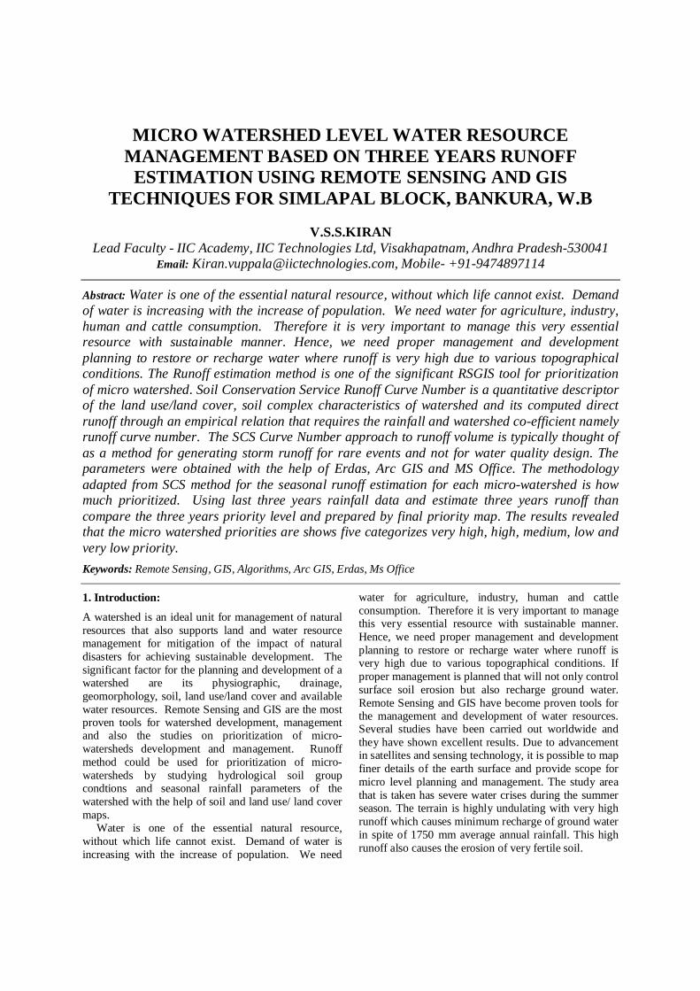
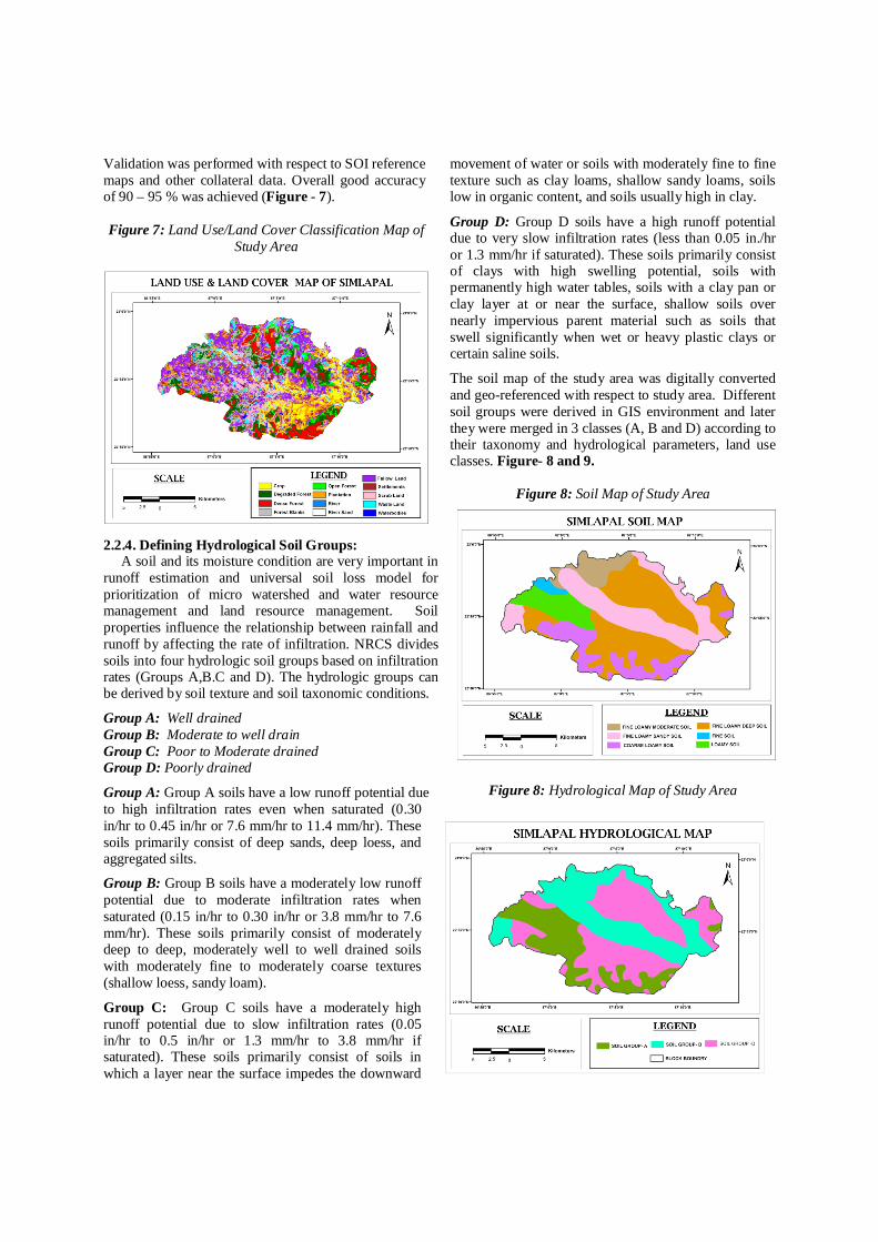
The drainage pattern formed the basis for divided into riverbanks, sub-watershed and micro-watershed. The texture of drainage pattern and its density not only define a geomorphic region but also indicate its cycle of erosion. The properties and pattern of a drainage basin are dependent upon a number of classes i.e. nature, distribution, features. The quantitative features of the drainage basin and its stream channel can be divided into linear aspect, aerial aspect and shape parameters.The study area was divided into 22 sub watershedshaving an area of 30 to 50 Sq kms and each sub watershed is further divided into micro-watershed having an area of 5 to 10 Sq kms or less the 5 Sqkms on the basis of drainage pattern and its texture.

Figure 3: Drainage Network Map of Study Area

Figure 4: Sub Watershed Map of Study Area

Figure 5: Micro Watershed Map of Study Area

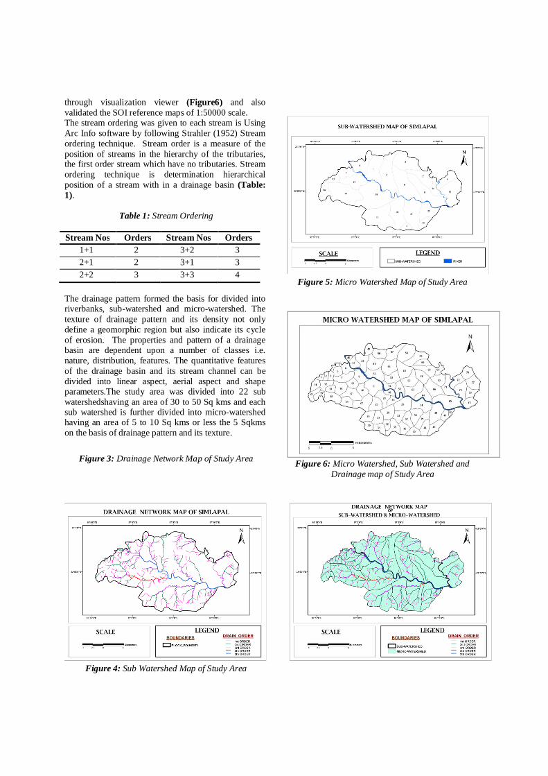
Figure 6: Micro Watershed, Sub Watershed and Drainage map of Study Area

Stream Nos Orders Stream Nos Orders 1+1 2 3+2 3 2+1 2 3+1 3 2+2 3 3+3 4

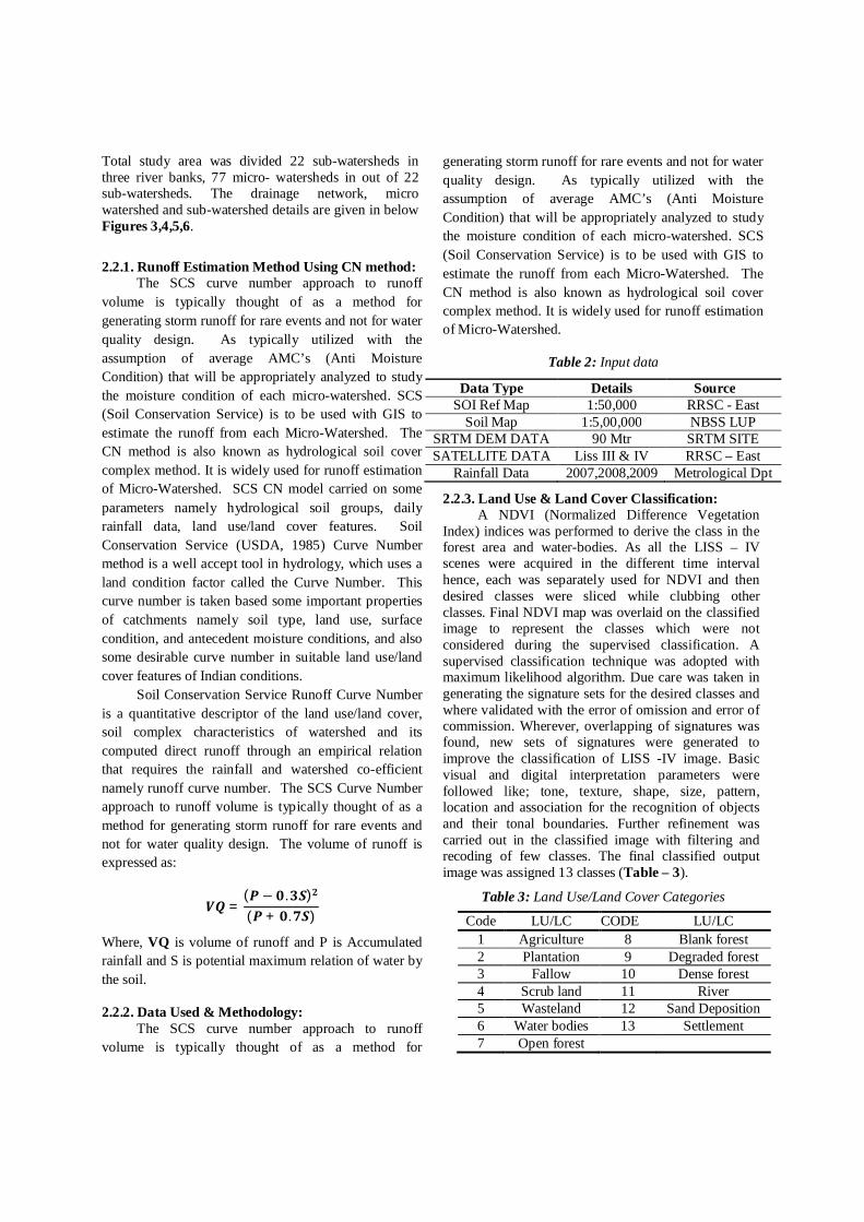
Total study area was divided 22 sub-watersheds in three river banks, 77 micro- watersheds in out of 22 sub-watersheds. The drainage network, micro watershed and sub-watershed details are given in below Figures 3,4,5,6.

2.2.1. Runoff Estimation Method Using CN method: The SCS curve number approach to runoff volume is typically thought of as a method for generating storm runoff for rare events and not for water quality design. As typically utilized with the assumption of average AMC’s (Anti Moisture Condition) that will be appropriately analyzed to study the moisture condition of each micro-watershed. SCS (Soil Conservation Service) is to be used with GIS to estimate the runoff from each Micro-Watershed. The CN method is also known as hydrological soil cover complex method. It is widely used for runoff estimation of Micro-Watershed. SCS CN model carried on some parameters namely hydrological soil groups, daily rainfall data, land use/land cover features. Soil Conservation Service (USDA, 1985) Curve Number method is a well accept tool in hydrology, which uses a land condition factor called the Curve Number. This curve number is taken based some important properties of catchments namely soil type, land use, surface condition, and antecedent moisture conditions, and also some desirable curve number in suitable land use/land cover features of Indian conditions. Soil Conservation Service Runoff Curve Number is a quantitative descriptor of the land use/land cover, soil complex characteristics of watershed and its computed direct runoff through an empirical relation that requires the rainfall and watershed co-efficient namely runoff curve number. The SCS Curve Number approach to runoff volume is typically thought of as a method for generating storm runoff for rare events and not for water quality design. The volume of runoff is expressed as:

푽푸 =(푷 − ퟎ.ퟑ푺)ퟐ

(푷 + ퟎ.ퟕ푺)

Where, VQ is volume of runoff and P is Accumulated rainfall and S is potential maximum relation of water by the soil.

2.2.2. Data Used & Methodology: The SCS curve number approach to runoff volume is typically thought of as a method for

generating storm runoff for rare events and not for water quality design. As typically utilized with the assumption of average AMC’s (Anti Moisture Condition) that will be appropriately analyzed to study the moisture condition of each micro-watershed. SCS (Soil Conservation Service) is to be used with GIS to estimate the runoff from each Micro-Watershed. The CN method is also known as hydrological soil cover complex method. It is widely used for runoff estimation of Micro-Watershed.

Table 2: Input data

Data Type Details Source SOI Ref Map 1:50,000 RRSC - East

Soil Map 1:5,00,000 NBSS LUP SRTM DEM DATA 90 Mtr SRTM SITE SATELLITE DATA Liss III & IV RRSC – East

Rainfall Data 2007,2008,2009 Metrological Dpt

2.2.3. Land Use & Land Cover Classification: A NDVI (Normalized Difference Vegetation Index) indices was performed to derive the class in the forest area and water-bodies. As all the LISS – IV scenes were acquired in the different time interval hence, each was separately used for NDVI and then desired classes were sliced while clubbing other classes. Final NDVI map was overlaid on the classified image to represent the classes which were not considered during the supervised classification. A supervised classification technique was adopted with maximum likelihood algorithm. Due care was taken in generating the signature sets for the desired classes and where validated with the error of omission and error of commission. Wherever, overlapping of signatures was found, new sets of signatures were generated to improve the classification of LISS -IV image. Basic visual and digital interpretation parameters were followed like; tone, texture, shape, size, pattern, location and association for the recognition of objects and their tonal boundaries. Further refinement was carried out in the classified image with filtering and recoding of few classes. The final classified output image was assigned 13 classes (Table – 3).

Table 3: Land Use/Land Cover Categories

Code LU/LC CODE LU/LC 1 Agriculture 8 Blank forest 2 Plantation 9 Degraded forest 3 Fallow 10 Dense forest 4 Scrub land 11 River 5 Wasteland 12 Sand Deposition 6 Water bodies 13 Settlement 7 Open forest

Validation was performed with respect to SOI reference maps and other collateral data. Overall good accuracy of 90 – 95 % was achieved (Figure - 7).

Figure 7: Land Use/Land Cover Classification Map of Study Area

2.2.4. Defining Hydrological Soil Groups: A soil and its moisture condition are very important in runoff estimation and universal soil loss model for prioritization of micro watershed and water resource management and land resource management. Soil properties influence the relationship between rainfall and runoff by affecting the rate of infiltration. NRCS divides soils into four hydrologic soil groups based on infiltration rates (Groups A,B.C and D). The hydrologic groups can be derived by soil texture and soil taxonomic conditions.

Group A: Well drained Group B: Moderate to well drain Group C: Poor to Moderate drained Group D: Poorly drained

Group A: Group A soils have a low runoff potential due to high infiltration rates even when saturated (0.30 in/hr to 0.45 in/hr or 7.6 mm/hr to 11.4 mm/hr). These soils primarily consist of deep sands, deep loess, and aggregated silts.

Group B: Group B soils have a moderately low runoff potential due to moderate infiltration rates when saturated (0.15 in/hr to 0.30 in/hr or 3.8 mm/hr to 7.6 mm/hr). These soils primarily consist of moderately deep to deep, moderately well to well drained soils with moderately fine to moderately coarse textures (shallow loess, sandy loam).

Group C: Group C soils have a moderately high runoff potential due to slow infiltration rates (0.05 in/hr to 0.5 in/hr or 1.3 mm/hr to 3.8 mm/hr if saturated). These soils primarily consist of soils in which a layer near the surface impedes the downward

movement of water or soils with moderately fine to fine texture such as clay loams, shallow sandy loams, soils low in organic content, and soils usually high in clay.

Group D: Group D soils have a high runoff potential due to very slow infiltration rates (less than 0.05 in./hr or 1.3 mm/hr if saturated). These soils primarily consist of clays with high swelling potential, soils with permanently high water tables, soils with a clay pan or clay layer at or near the surface, shallow soils over nearly impervious parent material such as soils that swell significantly when wet or heavy plastic clays or certain saline soils.

The soil map of the study area was digitally converted and geo-referenced with respect to study area. Different soil groups were derived in GIS environment and later they were merged in 3 classes (A, B and D) according to their taxonomy and hydrological parameters, land use classes. Figure- 8 and 9.

Figure 8: Soil Map of Study Area

Figure 8: Hydrological Map of Study Area

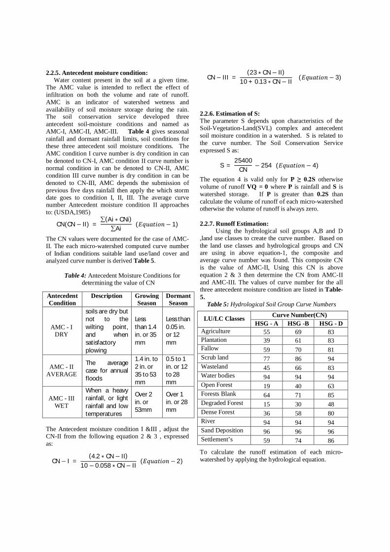
2.2.5. Antecedent moisture condition: Water content present in the soil at a given time. The AMC value is intended to reflect the effect of infiltration on both the volume and rate of runoff. AMC is an indicator of watershed wetness and availability of soil moisture storage during the rain. The soil conservation service developed three antecedent soil-moisture conditions and named as AMC-I, AMC-II, AMC-III. Table 4 gives seasonal rainfall and dormant rainfall limits, soil conditions for these three antecedent soil moisture conditions. The AMC condition I curve number is dry condition in can be denoted to CN-I, AMC condition II curve number is normal condition in can be denoted to CN-II, AMC condition III curve number is dry condition in can be denoted to CN-III, AMC depends the submission of previous five days rainfall then apply the which storm date goes to condition I, II, III. The average curve number Antecedent moisture condition II approaches to: (USDA,1985)

CN(CN− II) = (Ai ∗ CNi)

Ai (퐸푞푢푎푡푖표푛 − 1)

The CN values were documented for the case of AMC-II. The each micro-watershed computed curve number of Indian conditions suitable land use/land cover and analyzed curve number is derived Table 5.

Table 4: Antecedent Moisture Conditions for determining the value of CN

The Antecedent moisture condition I &III , adjust the CN-II from the following equation 2 & 3 , expressed as:

CN− I = (4.2 ∗ CN− II)

10 − 0.058 ∗ CN− II (퐸푞푢푎푡푖표푛 − 2)

CN− III = (23 ∗ CN− II)

10 + 0.13 ∗ CN− II (퐸푞푢푎푡푖표푛 − 3)

2.2.6. Estimation of S: The parameter S depends upon characteristics of the Soil-Vegetation-Land(SVL) complex and antecedent soil moisture condition in a watershed. S is related to the curve number. The Soil Conservation Service expressed S as:

S = 25400

CN − 254 (퐸푞푢푎푡푖표푛 − 4)

The equation 4 is valid only for P ≥ 0.2S otherwise volume of runoff VQ = 0 where P is rainfall and S is watershed storage. If P is greater than 0.2S than calculate the volume of runoff of each micro-watershed otherwise the volume of runoff is always zero. 2.2.7. Runoff Estimation: Using the hydrological soil groups A,B and D ,land use classes to create the curve number. Based on the land use classes and hydrological groups and CN are using in above equation-1, the composite and average curve number was found. This composite CN is the value of AMC-II, Using this CN is above equation 2 & 3 then determine the CN from AMC-II and AMC-III. The values of curve number for the all three antecedent moisture condition are listed in Table-5.

Table 5: Hydrological Soil Group Curve Numbers

To calculate the runoff estimation of each micro-watershed by applying the hydrological equation.

Antecedent Condition

Description Growing Season

Dormant Season

AMC - I DRY

soils are dry but not to the wilting point, and when satisfactory plowing

Less than 1.4 in. or 35 mm

Less than 0.05 in. or 12 mm

AMC - II AVERAGE

The average case for annual floods

1.4 in. to 2 in. or 35 to 53 mm

0.5 to 1 in. or 12 to 28 mm

AMC - III WET

When a heavy rainfall, or light rainfall and low temperatures

Over 2 in. or 53mm

Over 1 in. or 28 mm

LU/LC Classes Curve Number(CN) HSG - A HSG -B HSG - D

Agriculture 55 69 83 Plantation 39 61 83 Fallow 59 70 81 Scrub land 77 86 94 Wasteland 45 66 83 Water bodies 94 94 94 Open Forest 19 40 63 Forests Blank 64 71 85 Degraded Forest 15 30 48 Dense Forest 36 58 80 River 94 94 94 Sand Deposition 96 96 96 Settlement’s 59 74 86

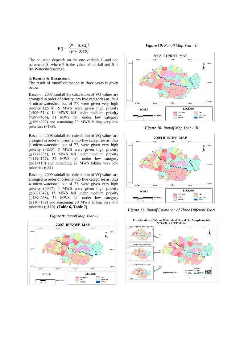
푽푄 =(푷 −ퟎ.ퟑ푺)ퟐ

(푷 + ퟎ.ퟕ푺)

The equation depends on the one variable P and one parameter S. where P is the value of rainfall and S is the Watershed storage. 3. Results & Discussion: The result of runoff estimation in three years is given below:

Based on 2007 rainfall the calculation of VQ values are arranged in order of priority into five categories as, thus 4 micro-watershed out of 77, were given very high priority (≥514), 5 MWS were given high priority (≥406<514), 14 MWS fall under medium priority (≥297<406), 31 MWS fall under low category (≥189<297) and remaining 23 MWS falling very low priorities (≤189).

Based on 2008 rainfall the calculation of VQ values are arranged in order of priority into five categories as, thus 2 micro-watershed out of 77, were given very high priority (≥235), 5 MWS were given high priority (≥177<235), 11 MWS fall under medium priority (≥119<177), 32 MWS fall under low category (≥61<119) and remaining 27 MWS falling very low priorities (≤61).

Based on 2009 rainfall the calculation of VQ values are arranged in order of priority into five categories as, thus 4 micro-watershed out of 77, were given very high priority (≥347), 4 MWS were given high priority (≥268<347), 15 MWS fall under medium priority (≥189<268), 34 MWS fall under low category (≥110<189) and remaining 20 MWS falling very low priorities (≤110). (Table 6, Table 7)

Figure 9: Runoff Map Year - I

Figure 10: Runoff Map Year - II

Figure 10: Runoff Map Year - III

Figure 11: Runoff Estimation of Three Different Years

3. Acknowledgements:

I want to express my sincere and heartfelt thanks to Regional Remote Sensing Centre-East, Kolkata, to provide the data and highly supporting me to analysis the work. 4. References:

Biswas et.al, 1999. Prioritization of Sub-watershed based on Morphometric Analysis of Drainage Basin: A remote sensing and GIS approach Journal of the Indian Society of Remote Sensing, 155-166.

USDA, SOIL CONSERVATION SERVICE(1985) , National Engineering Hand book, USA

Mr.Sachin, 2005, Prioritization of Micro-Watershed of Upper Bhama Basin on the Basis of Soil Erosion Risk Using Remote Sensing and GIS technology. Ph.D. Thesis, University of Pune, Department of Geography.

K. Nookaratnam et al., Y.K.Srivastava, V.VenkateswaraRao, E.Amminedu and K.S.R.Murthy, 2005. Check Dam positioning by prioritization of micro-watershed using SYI models and Morphometric Aanalysis : A remote sensing and GIS approach journal of Indian society of Remote Sensing, Vol 33, No.1

Chandramohan .T &Dilip G Durbude 2002. Estimation of soil erosion potential using universal soil loss equation journal of Indian society of remote sensing , vol 30 , No-4

S. K. Nag et al., 1998. Morphometric Analysis using Remote Sensing techniques in the Chakra sub-basin Purulia district,- journal of Indian Society of remote-sensing ,vol.26, no.1&2

Pramod Kumar et.al, K.N.Tiwari, D.K.Pal, 1991. Established SCS Runoff curve number from IRS digital

data base, journal of Indian Society of Remote Sensing ,vol.19,No.4,

Samah Al_Jabari et.al & Majed Abu Sharkh et.al, Ziad Al-Mimi,2009, Estimation of Runoff for agricultural watershed using SCS curve number and GIS, A remote sensing and GIS approach thirteenth International Water Technology Conference, IWTC 13,2009, Hurghada, Egypt,1213-1229.

A.A.KULKURNI et.al, S.P.Aggrawal&K.K.Das, Estimation of Surface Runoff using Rainfall-Runoff Modeling of Warasgaon Dam Catchment-a geospatial approach, downloaded site, (http:// www.gisdevelopment.net /application /nrm/water/surface/mi04081pf.htm) US department of Agricultural ,1981, Predicting rainfall erosion losses, A guide to conservation planning, handbook no 537 K. Uma Mahesh, 2007, Environment Impact Assessment of Dwarakeswar and Gandeshwari Reservoir Project, unpublished M. Tech thesis, IIT- Kgp.

JVS MURTHY. Watershed Management In India,21-34

Suresh. R, 1997. Soil and Water Conservation Engineering. Standard published distr., Delhi. 48-51 Smith and Wischmer, 1941, interpretation of Soil Conservation data for Field use. Agriculture Engineering, 173-175.

AshishPandey, P.P. Dabral, V.M. Chowdary, B.C.Mal. Estimation of Runoff for agricultural watershed using SCS Curve number and GIS.pg-1-5(downloaded site- http: //www.gisdevelopment.net / application/ agriculture /soil/mi0348pf/html

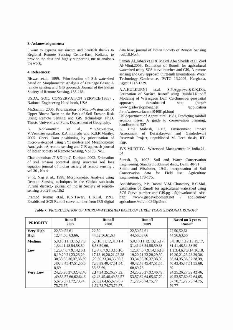
Table 7: PRIORITIZATION OF MICRO-WATERSHED BASEDON THREE YEARS SEASONAL RUNOFF

PRIORITY

Runoff 2007

Runoff 2008

Runoff 2009

Based on 3 years Runoff

Very High 22,50, 52,61 22,50 22,50,52,61 22,50,52,61 High 12,44,56, 63,66, 44,52,56,61,63 44,56,63,66 44,56,63,66 Medium 5,8,10,11,13,15,17,3

1,34,41,48,54,58,59 5,8,10,11,12,31,41,48,58,59,66,

5,8,10,11,12,13,15,17,31,41,48,54,58,59,68

5,8,10,11,12,13,15,17,31,41,48,54,58,59

Low 1,2,3,4,6,7,9,14,16,18,19,20,21,23,28,29,30,33,35,36,37,38,39,40,43,45,47,51,55,68,69

1,3,4,6,7,9,13,15,16,17,18,19,20,21,23,28,29,30,33,34,35,36,37,38,39,40,47,51,54,55,68,69,

1,2,3,4,6,7,9,14,16,18,19,20,21,23,28,29,30,33,34,35,36,37,38,39,40,42,43,45,47,51,55,60,69,76

1,2,3,4,6,7,9,14,16,18,19,20,21,23,28,29,30,33,34,35,36,37,38,39,40,43,45,47,51,55,68,69

Very Low 24,25,26,27,32,42,46,49,53,57,60,62,64,65,67,70,71,72,73,74,75,76,77,

2,14,24,25,26,27,32,42,43,45,46,49,53,57,60,62,64,65,67,70,71,72,73,74,75,76,77,

24,25,26,27,32,46,49,53,57,62,64,65,67,70,71,72,73,74,75,77

24,25,26,27,32,42,46,49,53,57,60,62,64,65,67,70,71,72,73,74,75,76,77

Table 6: Runoff Estimation Values of Three Different Years

MWS RUNOFF

MWS

RUNOFF 2007 2008 2009 2007 2008 2009

1 228.757424 70.0617351 145.24477 40 279.0162203 95.1699041 178.178248 2 210.2459787 55.2475589 135.764267 41 327.155152 119.732192 210.862499 3 273.3205871 92.4415226 174.220235 42 188.3732761 43.0773604 114.412552 4 222.7434212 64.0794906 142.693129 43 212.8372664 59.0178937 134.966588 5 347.8776517 130.275032 226.377677 44 506.2833144 212.574283 341.555399 6 264.9143039 88.3170547 168.513001 45 216.0619332 60.5870091 138.98248 7 235.8733898 72.7836603 151.076139 46 177.3920299 37.4629692 107.452861 8 384.3537398 152.216365 265.76938 47 273.6550681 92.6574999 174.567256 9 278.298629 94.9764803 177.795828 48 374.8914779 146.824015 248.721454

10 333.5444325 122.932666 215.569475 49 147.7725767 19.787855 89.0484738 11 382.7505801 152.321063 254.408317 50 604.9712134 271.759929 415.179315 12 407.2743935 165.66224 267.958144 51 244.1428796 76.8099649 155.967642 13 303.7561713 108.453383 193.93405 52 520.0878907 219.117351 352.155194 14 213.3224642 59.1843442 137.32804 53 141.5939302 15.5200531 79.3179161 15 299.3913298 105.804336 190.163081 54 298.628728 105.986222 190.142026 16 270.1509136 90.5478331 171.788382 55 218.5051047 62.0348807 140.783937 17 310.4196396 111.190213 198.45736 56 507.5979766 212.687854 341.730571 18 221.7407331 63.8925361 142.667183 57 82.76016492 3.05763508 32.99071 19 279.0162203 95.1699041 178.178248 58 328.2011429 120.033363 211.534737 20 248.402498 79.0497089 158.748431 59 344.1666522 124.985136 220.826618 21 221.7407331 63.8925361 142.667183 60 182.695658 40.620205 111.495079 22 623.2349943 291.733595 426.947102 61 537.3427592 229.3912 364.67714 23 236.1266146 72.7836603 151.043746 62 162.3414342 25.9041129 94.3505519 24 169.9819488 31.5000073 101.853055 63 492.8043069 206.160379 329.326047 25 167.5045565 29.7905498 99.823793 64 123.66127 11.0154947 71.7880279 26 161.6011339 28.0828584 97.0679217 65 180.7204559 39.3782336 110.140033 27 164.30685 29.6717596 99.9338538 66 424.8793026 173.735275 281.750297 28 247.8138896 78.8495291 158.554069 67 161.5561851 25.1296873 93.6577766 29 218.6625328 62.2113952 140.827008 68 296.8228837 105.839613 189.697389 30 240.5876829 74.8435331 153.483361 69 286.6045075 97.6110541 182.669399 31 333.0039211 122.988464 215.5326 70 141.7398479 15.45459 79.4028318 32 146.0704158 18.6569953 84.5515732 71 110.236288 7.71947342 56.34189 33 269.1956296 90.4387674 171.474467 72 161.4669894 25.2302447 93.5109024 34 297.9698589 105.894746 189.330015 73 99.29437395 8.43993397 41.2522588 35 239.791333 74.6692121 153.373976 74 151.7637125 20.2649444 86.6917024 36 265.5082239 88.2128948 168.486145 75 113.5818301 8.37479452 59.2572848 37 286.6045075 97.6110541 182.669399 76 188.2053266 42.9110866 114.421811 38 256.8133636 86.116129 164.25142 77 80.76101618 3.2817456 31.4027219 39 256.4882305 85.9491166 163.988705