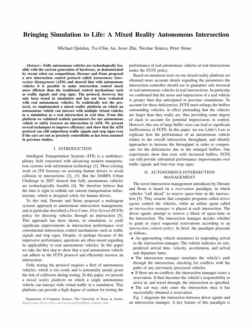
Bringing Simulation to Life: A Mixed Reality Autonomous Intersection

Michael Quinlan, Tsz-Chiu Au, Jesse Zhu, Nicolae Stiurca, Peter Stone

Abstract—Fully autonomous vehicles are technologically fea-sible with the current generation of hardware, as demonstratedby recent robot car competitions. Dresner and Stone proposeda new intersection control protocol called Autonomous Inter-section Management (AIM) and showed that with autonomousvehicles it is possible to make intersection control muchmore efficient than the traditional control mechanisms suchas traffic signals and stop signs. The protocol, however, hasonly been tested in simulation and has not been evaluatedwith real autonomous vehicles. To realistically test the pro-tocol, we implemented a mixed reality platform on which anautonomous vehicle can interact with multiple virtual vehiclesin a simulation at a real intersection in real time. From thisplatform we validated realistic parameters for our autonomousvehicle to safely traverse an intersection in AIM. We presentseveral techniques to improve efficiency and show that the AIMprotocol can still outperform traffic signals and stop signs evenif the cars are not as precisely controllable as has been assumedin previous studies.

I. INTRODUCTION

Intelligent Transportation Systems (ITS) is a multidisci-

plinary field concerned with advancing modern transporta-

tion systems with information technology [1]. Most existing

work on ITS focusses on assisting human drivers to avoid

collision in intersections [2], [3]. But the DARPA Urban

Challenge in 2007 showed that fully autonomous vehicles

are technologically feasible [4]. We therefore believe that

the time is right to rethink our current transportation infras-

tructure, which is designed solely for human drivers.

To this end, Dresner and Stone proposed a multiagent

systems approach to autonomous intersection management,

and in particular described a First Come, First Served (FCFS)

policy for directing vehicles through an intersection [5].

This approach has been shown, in simulation, to yield

significant improvements in intersection performance over

conventional intersection control mechanisms such as traffic

signals and stop signs. Despite, or perhaps because of the

impressive performance, questions are often raised regarding

its applicability to real autonomous vehicles. In this paper

we take the first step to show that a real autonomous vehicle

can adhere to the FCFS protocol and efficiently traverse an

intersection.

Fully testing the protocol requires a fleet of autonomous

vehicles, which is too costly and is potentially unsafe given

the risk of collisions during testing. In this paper, we present

a mixed reality platform on which a single autonomous

vehicle can interact with virtual traffic in a simulation. This

platform can provide a high degree of realism for testing the

Department of Computer Science, The University of Texas at Austin.{mquinlan,chiu,jzhu,nstiurca,pstone}@cs.utexas.edu

performance of real autonomous vehicles at real intersections

under the FCFS policy.

Based on numerous tests on our mixed reality platform we

obtained more accurate details regarding the parameters the

intersection controller should use to guarantee safe traversal

of real autonomous vehicles in real intersections. In particular

we confirmed that the noise and imprecision of a real vehicle

is greater than that anticipated in previous simulations. To

account for these deficiencies, FCFS must enlarge the buffers

surrounding vehicles, in effect pretending that the vehicles

are larger than they really are, thus providing some degree

of slack to account for potential imprecisions in control.

However, this use of large buffer sizes can lead to significant

inefficiencies in FCFS. In this paper, we use Little’s Law to

explicate how the performance of an autonomous vehicle

relates to the overall intersection throughput, and identify

approaches to increase the throughput in order to compen-

sate for the deficiencies due to the enlarged buffers. Our

experiments show that even with increased buffers, FCFS

can still provide substantial performance improvements over

traffic signals and four-way stop signs.

II. AUTONOMOUS INTERSECTION

MANAGEMENT

The novel intersection management introduced by Dresner

and Stone is based on a reservation paradigm, in which

vehicles “call ahead” to reserve space-time in the intersec-

tion [5]. They assume that computer programs called driver

agents control the vehicles, while an arbiter agent called

an intersection manager is placed at each intersection. The

driver agents attempt to reserve a block of space-time in

the intersection. The intersection manager decides whether

to grant or reject requested reservations according to an

intersection control policy. In brief, the paradigm proceeds

as follows.

• An approaching vehicle announces its impending arrival

to the intersection manager. The vehicle indicates its size,

predicted arrival time, velocity, acceleration, and arrival

and departure lanes.

• The intersection manager simulates the vehicle’s path

through the intersection, checking for conflicts with the

paths of any previously processed vehicles.

• If there are no conflicts, the intersection manager issues a

reservation. It then becomes the vehicle’s responsibility to

arrive at, and travel through, the intersection as specified.

• The car may only enter the intersection once it has

successfully obtained a reservation.

Fig. 1 diagrams the interaction between driver agents and

an intersection manager. A key feature of this paradigm is

that it relies only on vehicle-to-infrastructure (V2I) commu-

nication.1 In particular, the vehicles need not know anything

about each other beyond what is needed for local autonomous

control (e.g., to avoid running into the car in front). The

paradigm is also completely robust to communication dis-

ruptions: if a message is dropped, either by the intersection

manager or by the vehicle, delays may increase, but safety is

not compromised. Safety can also be guaranteed in scenarios

when both autonomous and human driven vehicles operate at

intersections. The intersection efficiency increases with the

ratio of autonomous vehicles to human driven vehicles in

such scenarios.

REQUEST

Intersection

Control Policy

REJECT

CONFIRM

Preprocess

Po

stp

roce

ss

Yes,

Restrictions

No, Reason

Driver

Agent

Intersection Manager

Fig. 1. Diagram of the intersection system.

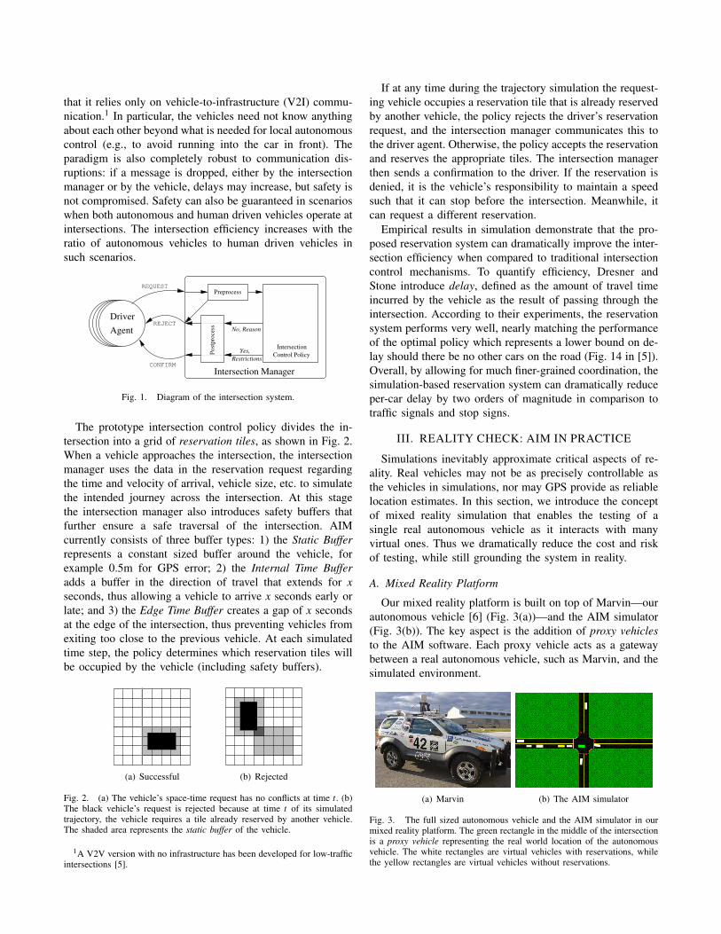
The prototype intersection control policy divides the in-

tersection into a grid of reservation tiles, as shown in Fig. 2.

When a vehicle approaches the intersection, the intersection

manager uses the data in the reservation request regarding

the time and velocity of arrival, vehicle size, etc. to simulate

the intended journey across the intersection. At this stage

the intersection manager also introduces safety buffers that

further ensure a safe traversal of the intersection. AIM

currently consists of three buffer types: 1) the Static Buffer

represents a constant sized buffer around the vehicle, for

example 0.5m for GPS error; 2) the Internal Time Buffer

adds a buffer in the direction of travel that extends for x

seconds, thus allowing a vehicle to arrive x seconds early or

late; and 3) the Edge Time Buffer creates a gap of x seconds

at the edge of the intersection, thus preventing vehicles from

exiting too close to the previous vehicle. At each simulated

time step, the policy determines which reservation tiles will

be occupied by the vehicle (including safety buffers).

(a) Successful (b) Rejected

Fig. 2. (a) The vehicle’s space-time request has no conflicts at time t. (b)The black vehicle’s request is rejected because at time t of its simulatedtrajectory, the vehicle requires a tile already reserved by another vehicle.The shaded area represents the static buffer of the vehicle.

1A V2V version with no infrastructure has been developed for low-trafficintersections [5].

If at any time during the trajectory simulation the request-

ing vehicle occupies a reservation tile that is already reserved

by another vehicle, the policy rejects the driver’s reservation

request, and the intersection manager communicates this to

the driver agent. Otherwise, the policy accepts the reservation

and reserves the appropriate tiles. The intersection manager

then sends a confirmation to the driver. If the reservation is

denied, it is the vehicle’s responsibility to maintain a speed

such that it can stop before the intersection. Meanwhile, it

can request a different reservation.

Empirical results in simulation demonstrate that the pro-

posed reservation system can dramatically improve the inter-

section efficiency when compared to traditional intersection

control mechanisms. To quantify efficiency, Dresner and

Stone introduce delay, defined as the amount of travel time

incurred by the vehicle as the result of passing through the

intersection. According to their experiments, the reservation

system performs very well, nearly matching the performance

of the optimal policy which represents a lower bound on de-

lay should there be no other cars on the road (Fig. 14 in [5]).

Overall, by allowing for much finer-grained coordination, the

simulation-based reservation system can dramatically reduce

per-car delay by two orders of magnitude in comparison to

traffic signals and stop signs.

III. REALITY CHECK: AIM IN PRACTICE

Simulations inevitably approximate critical aspects of re-

ality. Real vehicles may not be as precisely controllable as

the vehicles in simulations, nor may GPS provide as reliable

location estimates. In this section, we introduce the concept

of mixed reality simulation that enables the testing of a

single real autonomous vehicle as it interacts with many

virtual ones. Thus we dramatically reduce the cost and risk

of testing, while still grounding the system in reality.

A. Mixed Reality Platform

Our mixed reality platform is built on top of Marvin—our

autonomous vehicle [6] (Fig. 3(a))—and the AIM simulator

(Fig. 3(b)). The key aspect is the addition of proxy vehicles

to the AIM software. Each proxy vehicle acts as a gateway

between a real autonomous vehicle, such as Marvin, and the

simulated environment.

(a) Marvin (b) The AIM simulator

Fig. 3. The full sized autonomous vehicle and the AIM simulator in ourmixed reality platform. The green rectangle in the middle of the intersectionis a proxy vehicle representing the real world location of the autonomousvehicle. The white rectangles are virtual vehicles with reservations, whilethe yellow rectangles are virtual vehicles without reservations.

From the viewpoint of the intersection manager, the proxy

vehicle is identical to other virtual vehicles; the driver agent

on Marvin communicates with the intersection manager by

sending and receiving AIM messages via UDP. The motion

of the proxy vehicle, however, is controlled by Marvin, which

regularly updates the location, the direction, and the velocity

of the proxy vehicle via UDP packets containing the real-

time GPS information of the actual vehicle.

In our setup, we ran the AIM simulator adjacent to the

driver agent of Marvin on a computer located in Marvin. At

the beginning, the simulator generated potentially more than

100 virtual vehicles to create steady traffic in the simulated

world. Then the driver agent connected to the simulator and

the simulator created a proxy vehicle whose physical state

(the position, the direction, etc) was the same as Marvin’s.

As described above, the proxy vehicle interacted with other

virtual vehicles on behalf of Marvin. As Marvin approached

an intersection (and thus so did the proxy vehicle on the

simulator’s map), the driver agent sent a request message

over a specified UDP port to the proxy vehicle, which

then forwarded the message to the intersection manager in

the simulator. The intersection manager either accepted or

rejected the reservation request based on the virtual traffic

at the intersection. Once a reservation was granted, the

proxy vehicle forwarded the confirm message to Marvin, and

Marvin progressed through the intersection in both the real-

world and the simulated world accordingly. An example of

this experiment can be seen in the accompanying video.

B. Adjusting Simulation Parameters

The purpose of the mixed reality platform is to 1) test the

performance of AIM with real autonomous vehicles in real

world settings, and 2) identify aspects of the simulation that

failed to capture the true behavior of the real autonomous

vehicle. In this section, we present our findings and discuss

how we adjusted the simulation parameters to compensate

for the modeling errors for safe traversal in intersections.

Our tests were undertaken on a road with a legal speed

limit of 20 mph (8.94 m/s), for the safety of others the

maximum speed (Max Speed) of both Marvin and the virtual

vehicles were set to 7.5 m/s. The AIM simulator requires us

to define the operating characteristics of Marvin such as its

size and its maximum acceleration in order to compute its

trajectory in the intersection. Although Marvin is technically

capable of accelerating at 2.5 m/s2, the acceleration in

practice rarely exceeds 0.5 m/s2 due to driver discomfort

and the controller’s safety measures. Similarly, Marvin may

drift marginally below the speed limit for safety reasons and

to facilitate smoother braking when approaching a stop.

Apart from the operating characteristics of Marvin, we

need to choose the values for three additional parameters:

Static Buffer Size, Internal Time Buffer and Edge Time Buffer.

These parameters are used in AIM to factor in the GPS

errors and the vehicle controller’s errors due to sensor noise

and road conditions. We find that the default values of these

parameters (0.25, 0.0 and 0.5, respectively) in the simulator

are too small for Marvin since the errors in the real world

are much larger than the errors in simulation. Therefore, we

needed to figure out how large the buffer sizes should be

such that Marvin can stay inside the buffer during its entire

traversal. After a series of empirical test, we settled on the

following numbers: Static Buffer Size = 1 m, Internal Time

Buffer = 2 seconds and Edge Time Buffer = 4 seconds.

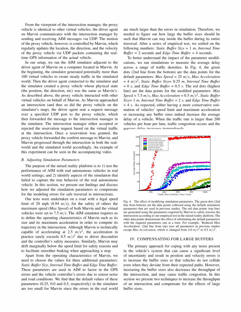
To better understand the impact of the parameter modifi-

cations, we ran simulations to measure the average delay

across a range of traffic densities. In Fig. 4, the green

dots (2nd line from the bottom) are the data points for the

default parameters: Max Speed = 25 m/s, Max Acceleration

= 4 m/s2, Static Buffer Size= 0.25 m, Internal Time Buffer

= 0 s, and Edge Time Buffer = 0.5 s. The red dots (highest

line) are the data points for the modified parameters: Max

Speed = 7.5 m/s, Max Acceleration = 0.5 m/s2, Static Buffer

Size= 1 m, Internal Time Buffer = 2 s, and Edge Time Buffer

= 4 s. As expected, either having a more conservative esti-

mation of vehicles’ speed limit and maximum acceleration

or increasing any buffer sizes indeed increase the average

delay of a vehicle. When the traffic rate is larger than 200

vehicles per hour per lane, traffic congestion occurs and the

average delay increases tremendously.

200 400 600 800 1000

Traffic Rate (vehicles / hour / lane)

0

50

100

150

200

250

300

Avera

ge D

ela

y (

secon

ds)

Vehicle Parameters

Reduced Max Accleration

Increased Time Buffer

Increased Edge Buffer

Increased Static Buffer

Default Paramters

Reduced Speed Limit

Fig. 4. The effect of modifying simulation parameters. The green dots (2ndline from bottom) are the data points collected using the default simulationparameters that are used in previous studies. The red data points (top line)are generated using the parameters required by Marvin to safely traverse theintersection according to our empirical test in the mixed reality platform. Theother data points demonstrate the effect of substituting the default parameterswith the required parameters one at a time. For example, ’Reduced MaxAcceleration’ (2nd line from top) uses all parameters in previous studiesexcept Max Acceleration, which is changed from 4.0 m/s2 to 0.5 m/s2.

IV. COMPENSATING FOR LARGE BUFFERS

The primary approach for coping with any noise present

in the vehicle’s system that can cause a significant level

of uncertainty and result in position and velocity errors is

to increase the buffer sizes so that vehicles do not collide

even when they deviate from their expected paths. However,

increasing the buffer sizes also decreases the throughput of

the intersection, and may cause traffic congestion. In this

section we present two techniques to increase the throughput

of an intersection and compensate for the effects of large

buffer sizes.

A. Static Buffer Sizes vs. Throughput

To understand how the buffer size affects the maximum

throughput characteristics of intersections, we borrow some

tools from queueing theory. An important result in queueing

theory is Little’s Law [7], which states that in a queueing

system the average arrival rate of customers, λ , is equal to

the average number of customers, T , in the system divided

by the average time, W , a customer spends in the system. In

the context of intersection management, Little’s Law can be

written as L = λW , where

• L is the average number of vehicles in the intersection;

• λ is the average arrival rate of the vehicles at the

intersection; and

• W is the average time a vehicle spends in the intersection.

Note that the arrival rate is equal to the throughput of the

system since no vehicle stalls inside an intersection.

Little’s Law shows that the maximum throughput (i.e., the

upper bound of λ ) an intersection can sustain is equal to the

upper bound of L divided by the lower bound of W , where

the upper bound of L is the maximum number of vehicles

that can coexist in an intersection, and the lower bound of

W is the minimum time a vehicle spends in the intersection.

Thus, Little’s Law shows that there are two ways to increase

the maximum throughput: 1) increase the average number

of vehicles in an intersection at any moment of time, and 2)

decrease the average time a vehicle spends in an intersection.

A trivial upper bound on L is the area of the intersection

divided by the average static buffer size of the vehicles.

But this bound is rather loose and in practice unachievable.

Nonetheless, it provides us some hints about the dependence

between the maximum throughput and the average static

buffer size of the vehicles. In general, an increase in static

buffer size has two effects: 1) the maximum number of

vehicles in each trajectory will decrease; and 2) the number

of nonintersecting trajectories decreases, since a large static

buffer effectively increases the width of the trajectories,

causing trajectories to overlap one another. In both cases,

the average number of vehicles decreases as the static buffer

size increases. According to Little’s Law, this can reduce

the throughput of an intersection. To see whether it is the

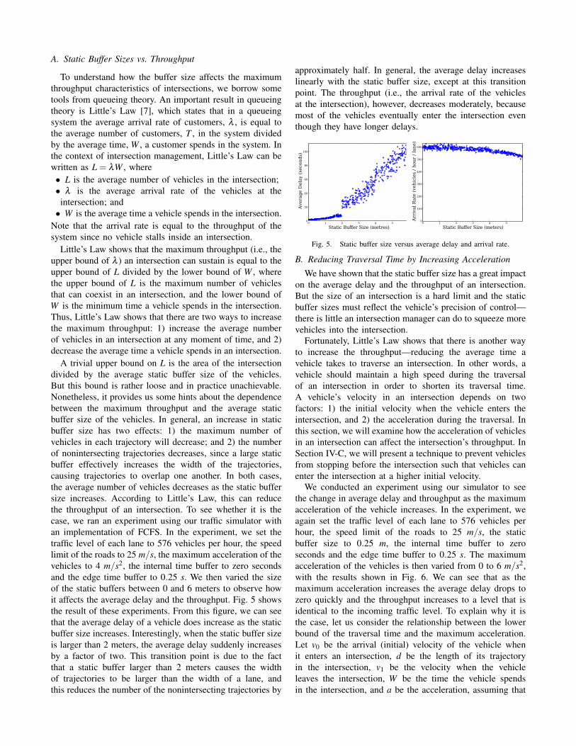
case, we ran an experiment using our traffic simulator with

an implementation of FCFS. In the experiment, we set the

traffic level of each lane to 576 vehicles per hour, the speed

limit of the roads to 25 m/s, the maximum acceleration of the

vehicles to 4 m/s2, the internal time buffer to zero seconds

and the edge time buffer to 0.25 s. We then varied the size

of the static buffers between 0 and 6 meters to observe how

it affects the average delay and the throughput. Fig. 5 shows

the result of these experiments. From this figure, we can see

that the average delay of a vehicle does increase as the static

buffer size increases. Interestingly, when the static buffer size

is larger than 2 meters, the average delay suddenly increases

by a factor of two. This transition point is due to the fact

that a static buffer larger than 2 meters causes the width

of trajectories to be larger than the width of a lane, and

this reduces the number of the nonintersecting trajectories by

approximately half. In general, the average delay increases

linearly with the static buffer size, except at this transition

point. The throughput (i.e., the arrival rate of the vehicles

at the intersection), however, decreases moderately, because

most of the vehicles eventually enter the intersection even

though they have longer delays.

0 1 2 3 4 5

Static Buffer Size (metres)

0

20

40

60

80

100

Avera

ge D

ela

y (

secon

ds)

0 1 2 3 4 5

Static Buffer Size (meters)

0

100

200

300

400

500

600

Arr

ival

Rate

(veh

icle

s /

hou

r /

lan

e)

Fig. 5. Static buffer size versus average delay and arrival rate.

B. Reducing Traversal Time by Increasing Acceleration

We have shown that the static buffer size has a great impact

on the average delay and the throughput of an intersection.

But the size of an intersection is a hard limit and the static

buffer sizes must reflect the vehicle’s precision of control—

there is little an intersection manager can do to squeeze more

vehicles into the intersection.

Fortunately, Little’s Law shows that there is another way

to increase the throughput—reducing the average time a

vehicle takes to traverse an intersection. In other words, a

vehicle should maintain a high speed during the traversal

of an intersection in order to shorten its traversal time.

A vehicle’s velocity in an intersection depends on two

factors: 1) the initial velocity when the vehicle enters the

intersection, and 2) the acceleration during the traversal. In

this section, we will examine how the acceleration of vehicles

in an intersection can affect the intersection’s throughput. In

Section IV-C, we will present a technique to prevent vehicles

from stopping before the intersection such that vehicles can

enter the intersection at a higher initial velocity.

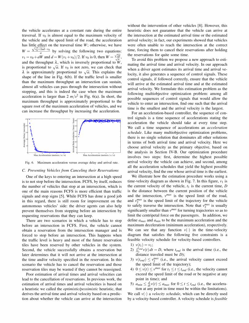
We conducted an experiment using our simulator to see

the change in average delay and throughput as the maximum

acceleration of the vehicle increases. In the experiment, we

again set the traffic level of each lane to 576 vehicles per

hour, the speed limit of the roads to 25 m/s, the static

buffer size to 0.25 m, the internal time buffer to zero

seconds and the edge time buffer to 0.25 s. The maximum

acceleration of the vehicles is then varied from 0 to 6 m/s2,

with the results shown in Fig. 6. We can see that as the

maximum acceleration increases the average delay drops to

zero quickly and the throughput increases to a level that is

identical to the incoming traffic level. To explain why it is

the case, let us consider the relationship between the lower

bound of the traversal time and the maximum acceleration.

Let v0 be the arrival (initial) velocity of the vehicle when

it enters an intersection, d be the length of its trajectory

in the intersection, v1 be the velocity when the vehicle

leaves the intersection, W be the time the vehicle spends

in the intersection, and a be the acceleration, assuming that

the vehicle accelerates at a constant rate during the entire

traversal. If v0 is almost equal to the maximum velocity of

the vehicle and the speed limit of the road, the acceleration

has little effect on the traversal time W ; otherwise, we have

W =

√v2

0+2ad−v0

aby solving the following two equations:

v1 = v0+aW and d =W (v1+v0)/2. If v0 is 0, then W =√

2d√a

,

and the throughput λ , which is inversely proportional to W ,

is proportional to√

a. If v0 is not zero, we can check that

λ is approximately proportional to√

a. This explains the

shape of the line in Fig. 6(b). If the traffic level is smaller

than the maximum throughput an intersection can sustain,

almost all vehicles can pass through the intersection without

stopping, and this is indeed the case when the maximum

acceleration is larger than 2 m/s2 in Fig. 6(a). In short, the

maximum throughput is approximately proportional to the

square root of the maximum acceleration of vehicles, and we

can increase the throughput by increasing the acceleration.

0 1 2 3 4 5

Max Acceleration (meters / s / s)

0

50

100

150

200

250

Avera

ge D

ela

y (

secon

ds)

0 1 2 3 4 5

Max Acceleration (meters / s / s)

0

100

200

300

400

500

600

Arr

ival

Rate

(veh

icle

s /

hou

r /

lan

e)

Fig. 6. Maximum acceleration versus average delay and arrival rate.

C. Preventing Vehicles from Canceling their Reservations

One of the keys to entering an intersection at a high speed

is to not stop before the intersection. FCFS, by itself, reduces

the number of vehicles that stop at an intersection, which is

one of the main reasons FCFS is more efficient than traffic

signals and stop signs [5]. While FCFS has done a good job

in this regard, there is still room for improvement on the

autonomous vehicles’ side: the driver agents can also help

prevent themselves from stopping before an intersection by

requesting reservations that they can keep.

There are two scenarios in which a vehicle has to stop

before an intersection in FCFS. First, the vehicle cannot

obtain a reservation from the intersection manager and is

forced to stop before an intersection. This happens when

the traffic level is heavy and most of the future reservation

tiles have been reserved by other vehicles in the system.

Second, the vehicle successfully obtains a reservation but

later determines that it will not arrive at the intersection at

the time and/or velocity specified in the reservation. In this

scenario the vehicle has to cancel the reservation and those

reservation tiles may be wasted if they cannot be reassigned.

Poor estimation of arrival times and arrival velocities can

lead to the cancellation of reservations. In previous work, the

estimation of arrival times and arrival velocities is based on

a heuristic we called the optimistic/pessimistic heuristic, that

derives the arrival time and arrival velocity based on a predic-

tion about whether the vehicle can arrive at the intersection

without the intervention of other vehicles [8]. However, this

heuristic does not guarantee that the vehicle can arrive at

the intersection at the estimated arrival time or the estimated

arrival velocity; in fact, our experiments showed that vehicles

were often unable to reach the intersection at the correct

time, forcing them to cancel their reservations after holding

the reservations for quite some time.

To avoid this problem we propose a new approach to esti-

mating the arrival time and arrival velocity. In our approach

when a driver agent estimates its arrival time and arrival ve-

locity, it also generates a sequence of control signals. These

control signals, if followed correctly, ensure that the vehicle

will arrive at the estimated arrival time and at the estimated

arrival velocity. We formulate this estimation problem as the

following multiobjective optimization problem: among all

possible sequences of control signals that would allow the

vehicle to enter an intersection, find one such that the arrival

time is the smallest and the arrival velocity is the largest.

For an acceleration-based controller, the sequence of con-

trol signals is a time sequence of accelerations stating the

acceleration the vehicle should take at every time step.

We call a time sequence of accelerations an acceleration

schedule. Like many multiobjective optimization problems,

there is no single solution that dominates all other solutions

in terms of both arrival time and arrival velocity. Here we

choose arrival velocity as the primary objective, based on

the analysis in Section IV-B. Our optimization procedure

involves two steps: first, determine the highest possible

arrival velocity the vehicle can achieve, and second, among

all the acceleration schedules that yield the highest possible

arrival velocity, find the one whose arrival time is the earliest.

We illustrate how the estimation procedure works using a

time-velocity diagram as shown in Fig. 7. In this figure, v1 is

the current velocity of the vehicle, t1 is the current time, D

is the distance between the current position of the vehicle

and the intersection, vmax is the speed limit of the road,

and vmax2 is the speed limit of the trajectory for the vehicle

to safely traverse the intersection. Note that vmax2 is usually

significantly smaller than vmax for turning trajectories so as to

limit the centripetal force on the passengers. In addition, we

define amax and amin to be the maximum acceleration and the

maximum deceleration (minimum acceleration), respectively.

We can see that any function v(·) in the time-velocity

diagram that satisfies the following five constraints is a

feasible velocity schedule for velocity-based controllers.

1) v(t1) = v1;

2)∫ tend

t1v(t)dt = D, where tend is the arrival time (i.e., the

distance traveled must be D);

3) v(tend) ≤ vmax2 (i.e., the arrival velocity cannot exceed

the speed limit of the trajectory);

4) 0 ≤ v(t)≤ vmax for t1 ≤ t ≤ tend (i.e., the velocity cannot

exceed the speed limit of the road or be negative at any

point in time); and

5) amin ≤ ddt

v(t)≤ amax for 0 ≤ t ≤ tend (i.e., the accelera-

tion at any point in time must be within the limitations).

We call v(·) a velocity schedule, which can be directly used

by a velocity-based controller. A velocity schedule is feasible

if it satisfies the above constraints. Our objective is to find a

feasible velocity schedule v(·) such that v(tend) is as high as

possible while tend is as small as possible. For acceleration-

based controllers, we can compute the corresponding feasible

acceleration schedule by the derivative of v(·) (i.e., ddt

v(t)).

Velocity

Time

v1

v2max

vmax

Area1 Area2 Area3

t2 t3t1 tend

(a) Case 1: Area1 +Area3 ≤ D

Velocity

Time

v1

v2max

vmax

Area4 Area5

vtop

t4t1 tend

(b) Case 2: Area1+Area3 >D

Fig. 7. The time-velocity diagrams for the estimation of the arrival timeand the arrival velocity.

We propose an optimization procedure to find v(·) with

the highest possible v(tend) and smallest tend . First, compute

the area of two trapezoids Area1 and Area3 as shown in

Fig. 7(a). To compute Area1, find a point (t2,vmax) such

that (t2,vmax) is an interception of the line extending from

(t1,v1) with slope amax and the horizontal line v = vmax. We

compute Area3 by choosing an arrival time t ′end and then find

an intercepting point (t ′3,vmax) between the line v = vmax and

the line passing through the point (t ′end ,vmax2 ) with slope amin.

If Area1 +Area3 ≤ D, the vehicle can accelerate to vmax,

maintain that speed for a certain period of time, then de-

celerate to vmax2 , and finally reach the intersection (Case

1 in Fig. 7). Then Area2 = D − Area1 − Area3 is non-

negative. Let d beArea2vmax . Then we can determine the actual

value of t ′3 and t ′end by t3 = t2 + d and tend = t3 +2×Area3

vmax+vmax2

.

From this the optimization procedure can find a piecewise

linear function for v(·) such that v(·) is a feasible velocity

schedule. The optimization procedure returns the acceleration

schedule 〈(t1,amax),(t2,0),(t3,amin)〉. If Area1 +Area3 > D,

the vehicle cannot accelerate to vmax because D is too small.

But the vehicle can still accelerate to a velocity vtop that is

less than the speed limit vmax and immediately decelerate to

vmax2 if vtop exists (Case 2 in Fig. 7). However, if vtop does not

exist and v1 > vmax2 , there is no feasible acceleration schedule

since the vehicle is too close to the intersection.

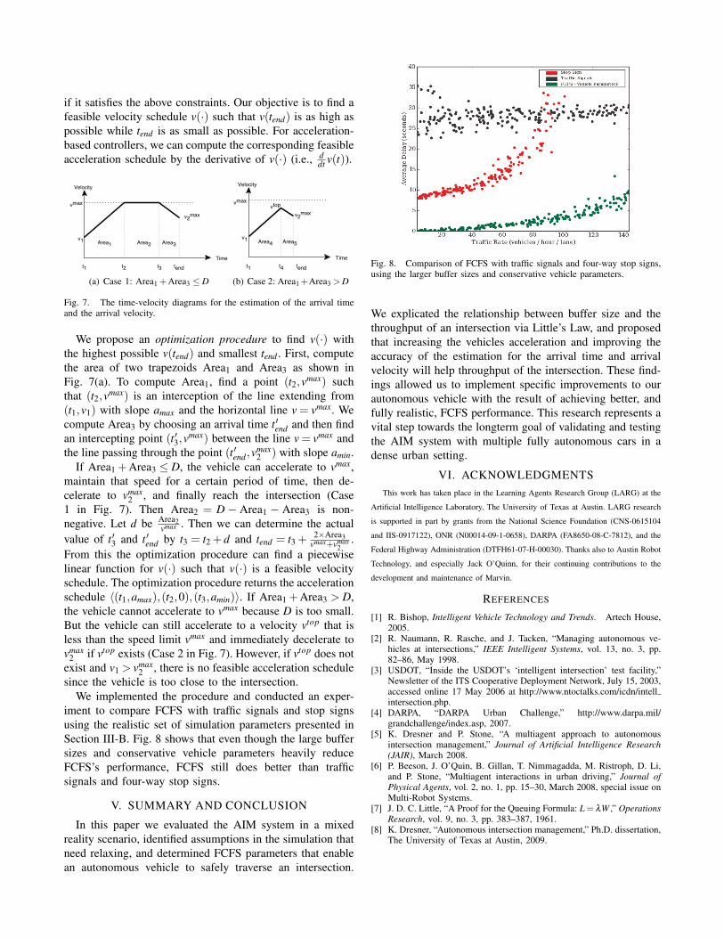
We implemented the procedure and conducted an exper-

iment to compare FCFS with traffic signals and stop signs

using the realistic set of simulation parameters presented in

Section III-B. Fig. 8 shows that even though the large buffer

sizes and conservative vehicle parameters heavily reduce

FCFS’s performance, FCFS still does better than traffic

signals and four-way stop signs.

V. SUMMARY AND CONCLUSION

In this paper we evaluated the AIM system in a mixed

reality scenario, identified assumptions in the simulation that

need relaxing, and determined FCFS parameters that enable

an autonomous vehicle to safely traverse an intersection.

Fig. 8. Comparison of FCFS with traffic signals and four-way stop signs,using the larger buffer sizes and conservative vehicle parameters.

We explicated the relationship between buffer size and the

throughput of an intersection via Little’s Law, and proposed

that increasing the vehicles acceleration and improving the

accuracy of the estimation for the arrival time and arrival

velocity will help throughput of the intersection. These find-

ings allowed us to implement specific improvements to our

autonomous vehicle with the result of achieving better, and

fully realistic, FCFS performance. This research represents a

vital step towards the longterm goal of validating and testing

the AIM system with multiple fully autonomous cars in a

dense urban setting.

VI. ACKNOWLEDGMENTS

This work has taken place in the Learning Agents Research Group (LARG) at the

Artificial Intelligence Laboratory, The University of Texas at Austin. LARG research

is supported in part by grants from the National Science Foundation (CNS-0615104

and IIS-0917122), ONR (N00014-09-1-0658), DARPA (FA8650-08-C-7812), and the

Federal Highway Administration (DTFH61-07-H-00030). Thanks also to Austin Robot

Technology, and especially Jack O’Quinn, for their continuing contributions to the

development and maintenance of Marvin.

REFERENCES

[1] R. Bishop, Intelligent Vehicle Technology and Trends. Artech House,2005.

[2] R. Naumann, R. Rasche, and J. Tacken, “Managing autonomous ve-hicles at intersections,” IEEE Intelligent Systems, vol. 13, no. 3, pp.82–86, May 1998.

[3] USDOT, “Inside the USDOT’s ‘intelligent intersection’ test facility,”Newsletter of the ITS Cooperative Deployment Network, July 15, 2003,accessed online 17 May 2006 at http://www.ntoctalks.com/icdn/intellintersection.php.

[4] DARPA, “DARPA Urban Challenge,” http://www.darpa.mil/grandchallenge/index.asp, 2007.

[5] K. Dresner and P. Stone, “A multiagent approach to autonomousintersection management,” Journal of Artificial Intelligence Research

(JAIR), March 2008.[6] P. Beeson, J. O’Quin, B. Gillan, T. Nimmagadda, M. Ristroph, D. Li,

and P. Stone, “Multiagent interactions in urban driving,” Journal of

Physical Agents, vol. 2, no. 1, pp. 15–30, March 2008, special issue onMulti-Robot Systems.

[7] J. D. C. Little, “A Proof for the Queuing Formula: L= λW ,” Operations

Research, vol. 9, no. 3, pp. 383–387, 1961.[8] K. Dresner, “Autonomous intersection management,” Ph.D. dissertation,

The University of Texas at Austin, 2009.