A novel workflow for seismic net pay estimation with uncertaintyMichael E. Glinsky,1 Dale Baptiste,1 Muhlis Unaldi,1 and Vishal Nagassar21)Geotrace Technologies, Houston, TX, USA2)Centrica E&P, Port of Spain, Trinidad

This paper presents a novel workflow for seismic net pay estimation with uncertainty. It is demonstrated onthe Cassra/Iris Field. The theory for the stochastic wavelet derivation (which estimates the seismic noise levelalong with the wavelet, time-to-depth mapping, and their uncertainties), the stochastic sparse spike inversion,and the net pay estimation (using secant areas) along with its uncertainty; will be outlined. This includesbenchmarking of this methodology on a synthetic model. A critical part of this process is the calibration of thesecant areas. This is done in a two step process. First, a preliminary calibration is done with the stochasticreflection response modeling using rock physics relationships derived from the well logs. Second, a refinementis made to the calibration to account for the encountered net pay at the wells. Finally, a variogram structure isestimated from the extracted secant area map, then used to build in the lateral correlation to the ensemble ofnet pay maps while matching the well results to within the nugget of the variogram. These net pay maps arethen integrated, over the area of full saturation gas, to give the GIIP distribution (Gaussian distributions forthe porosity, gas expansion factor, and gas saturation for the sand end member are assumed and incorporatedin the estimate of GIIP). The method is demonstrated on the Iris (UP5 turbidite) interval. The net pay iscorrected for reduction in the amplitudes over part of the area due to shallow gas. The sensitivity of the GIIPto the independent stochastic variables is estimated (determining the value of information) so that businessdecisions can be made that maximize the value of the field.

I. INTRODUCTION

This paper presents the initial implementation anddemonstration of a novel work flow. Certain partsare established technology using previously developed,but not widely used methods (i.e., stochastic waveletderivation, sparse spike inversion based on the ideas ofDaubechies and Mallat, net pay estimation using secantarea, stochastic reflection response modeling using rockphysics relationships derived from well logs, and geosta-tistical simulation of lateral correlation taking into ac-count well measurements). This not withstanding, sig-nificant development was needed to assimilate these ca-pabilities in an integrated workflow. Other parts werenovel technology that was developed and applied for thefirst time (i.e., the stochastic aspect of the sparse spikeinversion and the net pay estimation).

The details and synthetic benchmarking of this tech-nology suite will be discussed in Sec. II. More specifi-cally, the wavelet derivation and seismic noise estimationwill be discussed in Sec. II A, the novel stochastic sparsespike inversion will be discussed in Sec. II B, the secantamplitude extraction and stochastic net pay estimation(that is, net pay with uncertainty) will be discussed inSec. II C, the two step calibration process that includesthe stochastic reflection response modeling will be dis-cussed in Sec. II D, and how the lateral correlation andwell measurements of net pay are built into the ensembleof net pay estimates will be discussed in Sec. II E.

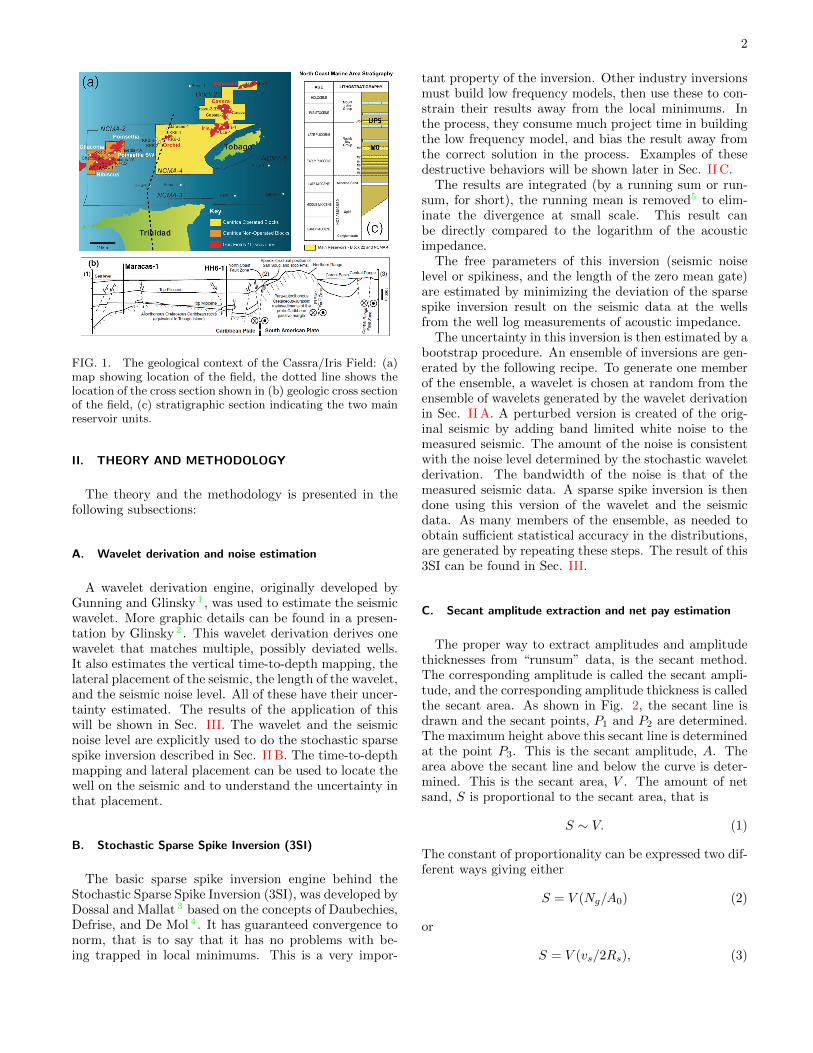
This methodology will be demonstrated on theCassra/Iris Field. These licenses (Block 22 and NCMA-4) lie on the regional Patao High basement structure lo-cated within the West Tobago Basin, offshore the northcoast of Trinidad and to the northwest coast of Tobago(see Fig. 1). The area contains primarily upper Mioceneto Pleistocene aged clastic sediments resting on a hetero-

geneous basement of Jurassic/Cretaceous age consistingof metamorphic and igneous rocks.

In the Block 22 license, the Cassra gas discovery iscontained in the uppermost early Pliocene M0 reservoirsands. In NCMA-4, the Iris gas discovery is in Pleis-tocene aged reservoir sands, termed UP5. The hydrocar-bon system consists of mainly combination structural-stratigraphic traps, formed by compactional drape overbasement structural highs, which are sealed by intra-formational shales/silts that also provide the dry biogenicgas source for all the gas discoveries and producing fieldsof the basin.

Cassra is the main discovered resource in Block 22 withthe resource area being clearly defined on 3D seismic dataas a strong amplitude anomaly covering around 60 km2.The trap is a combination structural-stratigraphic trap ingood quality reservoir sands of early Pliocene age, knownlocally as the M0 reservoir. Strong clinoformal geome-tries are seen on seismic and attest to the progradationof smaller-scale “parasquence-set” within the overall sandbody unit.

Iris straddles the boundary between licenses NCMA-4 and Block 22 and the Iris field is clearly definedon 3D seismic data as a strong amplitude anomaly,covering around 100 km2. The trap is a combinationstructural-stratigraphic trap in Pleistocene aged sands,locally termed UP5, which are interpreted as a deep wa-ter channel-lobe complex.

Section III presents the results of the analysis on theturbidite sequences of the UP5/Iris interval. The volu-metric distribution is corrected for a reduction in ampli-tude over part of the area due to shallow gas.

arX

iv:1

604.

0044

1v1

[ph

ysic

s.ge

o-ph

] 2

Apr

201

6

2

FIG. 1. The geological context of the Cassra/Iris Field: (a)map showing location of the field, the dotted line shows thelocation of the cross section shown in (b) geologic cross sectionof the field, (c) stratigraphic section indicating the two mainreservoir units.

II. THEORY AND METHODOLOGY

The theory and the methodology is presented in thefollowing subsections:

A. Wavelet derivation and noise estimation

A wavelet derivation engine, originally developed byGunning and Glinsky 1 , was used to estimate the seismicwavelet. More graphic details can be found in a presen-tation by Glinsky 2 . This wavelet derivation derives onewavelet that matches multiple, possibly deviated wells.It also estimates the vertical time-to-depth mapping, thelateral placement of the seismic, the length of the wavelet,and the seismic noise level. All of these have their uncer-tainty estimated. The results of the application of thiswill be shown in Sec. III. The wavelet and the seismicnoise level are explicitly used to do the stochastic sparsespike inversion described in Sec. II B. The time-to-depthmapping and lateral placement can be used to locate thewell on the seismic and to understand the uncertainty inthat placement.

B. Stochastic Sparse Spike Inversion (3SI)

The basic sparse spike inversion engine behind theStochastic Sparse Spike Inversion (3SI), was developed byDossal and Mallat 3 based on the concepts of Daubechies,Defrise, and De Mol 4 . It has guaranteed convergence tonorm, that is to say that it has no problems with be-ing trapped in local minimums. This is a very impor-

tant property of the inversion. Other industry inversionsmust build low frequency models, then use these to con-strain their results away from the local minimums. Inthe process, they consume much project time in buildingthe low frequency model, and bias the result away fromthe correct solution in the process. Examples of thesedestructive behaviors will be shown later in Sec. II C.

The results are integrated (by a running sum or run-sum, for short), the running mean is removed5 to elim-inate the divergence at small scale. This result canbe directly compared to the logarithm of the acousticimpedance.

The free parameters of this inversion (seismic noiselevel or spikiness, and the length of the zero mean gate)are estimated by minimizing the deviation of the sparsespike inversion result on the seismic data at the wellsfrom the well log measurements of acoustic impedance.

The uncertainty in this inversion is then estimated by abootstrap procedure. An ensemble of inversions are gen-erated by the following recipe. To generate one memberof the ensemble, a wavelet is chosen at random from theensemble of wavelets generated by the wavelet derivationin Sec. II A. A perturbed version is created of the orig-inal seismic by adding band limited white noise to themeasured seismic. The amount of the noise is consistentwith the noise level determined by the stochastic waveletderivation. The bandwidth of the noise is that of themeasured seismic data. A sparse spike inversion is thendone using this version of the wavelet and the seismicdata. As many members of the ensemble, as needed toobtain sufficient statistical accuracy in the distributions,are generated by repeating these steps. The result of this3SI can be found in Sec. III.

C. Secant amplitude extraction and net pay estimation

The proper way to extract amplitudes and amplitudethicknesses from “runsum” data, is the secant method.The corresponding amplitude is called the secant ampli-tude, and the corresponding amplitude thickness is calledthe secant area. As shown in Fig. 2, the secant line isdrawn and the secant points, P1 and P2 are determined.The maximum height above this secant line is determinedat the point P3. This is the secant amplitude, A. Thearea above the secant line and below the curve is deter-mined. This is the secant area, V . The amount of netsand, S is proportional to the secant area, that is

S ∼ V. (1)

The constant of proportionality can be expressed two dif-ferent ways giving either

S = V (Ng/A0) (2)

or

S = V (vs/2Rs), (3)

3

FIG. 2. Secant amplitude extraction: (a) location of thethree secant points shown as horizons on a cross section ofacoustic impedance from a sparse spike inversion. Shown isthe original seismic data as the black wiggles. The false colorimage is the acoustic impedance of the sparse spike inversionusing a rainbow colorbar where soft impedances are the hotred colors and the hard acoustic impedances are the cool bluecolors, (b) a seismic trace showing the secant line, improperdashed secant lines that attempt to separate the two sandunits, the location of the three secant points, the secant am-plitude A, and the grey secant area V .

where Ng is the average net-to-gross of the sand, A0 is theaverage secant amplitude for regions of the sand abovetuning, vs is the average velocity of the sand, and Rsis the average modeled reflection coefficient of the endmember sand. Eq. (2) is best used when there are nowell penetrations of the objective, that is a rank explo-ration case. An initial estimate in the appraisal case canbe estimated by Eq. (3), where vs and Rs are both esti-mated from the stochastic reflection modeling of the rockphysics relationships. The appraisal calibration proce-dure will be discussed in more detail in Sec. II D. A verygood, unbiased estimate of net sand will be shown.

It should be noted in Fig. 2 that the secant area iscalculated over the total package. If small sands thatare interfering with each other have their amplitudes andareas extracted separately, there will be a significant errormade as demonstrated by the dashed lines in the figure.

An advantage in using secant area is that it is insensi-tive to phase, up to first order in the error in the phase.It is also an intensive property, not an extensive prop-erty like a root mean square (RMS) amplitude. In other

FIG. 3. Synthetic model used to benchmark the sparse spikeinversion, secant area extraction and the net sand calcula-tion: (a) the structure of the model, (b) the synthetic seismicsection.

words, the amplitude is not dependent on the length orchoice of the interval. The secant points are uniquelydefined and can be determined as part of the algorithm,where the the end points for the RMS are determinedoutside the algorithm by the analyst. This makes theRMS amplitude dependent both on the choice of gateand the width of the sand.

To benchmark this procedure and the various differenttypes of sparse spike inversions, the model shown in Fig.3 was constructed. It is a soft, type III sand, characteris-tic of the U.S. Gulf of Mexico plio-pleistocene, imbeddedin a uniform shale with a shale lens. The maximum thick-ness of this shale lens, and the thickness of the sand oneither side of this lens at the maximum lens thickness wasset to be exactly the tuning thickness of the 20 Hz Richterwavelet used to generate the synthetic seismic. This wasdone to present the greatest challenge to the sparse spikeinversions. The result of the secant amplitude extractionon the “runsum” data before and after the sparse spikeinversion that we have used are shown in Fig. 4. Notethe tuning enhancement before the inversion, and howthe inversion has removed that resonance. The A0 wasestimated from this figure, then the secant area extrac-tion along with Eq. (2) was used to calculate the netsand. The result is shown in Fig. 5. This was done forthe original seismic data, our sparse spike inversion, andtwo common industry inversions. Notice the dramaticimprovement from the initial seismic data to our sparsespike inversion. The match of our sparse spike inversionto the true answer is nearly perfect. The same can notbe said for the other two industry inversions. Both sufferfrom local minimums and the bias introduced by the lowfrequency model used to avoid them.

D. Calibration

The calibration was done in two steps. The prelim-inary calibration consisted of stochastic reflection mod-eling given the rock physics relationships. The average

4

FIG. 4. Secant amplitude extraction of the synthetic modelshown in Fig. 3: (a) extraction from the un-inverted runsumdata. The correct amplitude is shown as the yellow line andA0, (b) extraction from the sparse spike inverted data.

sand velocity, vs, and the average reflection coefficient forthe end member sand, Rs, were calculated then substi-tuted into Eq. (3) to generate the net sand map.

The well logs were first analyzed to determine the rockphysics relationships. For this analysis a set of intervalswere picked by hand that are characteristic of the end-member lithologies, as shown in Fig. 6. A set of linearrelationships of the form

vp = Avp +Bvp TVDBML + Cvp LFIV + σvp, (4)

vs = Avs +Bvsvp + σvs, (5)

and

ρ = Aρ +Bρvp + σρ. (6)

were fit to the acoustic properties, where TVDBML isTotal Vertical Depth Below Mud Line, LFIV is LowFrequency Interval Velocity (practically will be seismicimaging velocity, but is a 250 m average of the sonicvelocity in this regression), and the σ’s are the uncer-tainties in the fits. Equation (6) is often called theGardner-Gardner-Gregory relationship6, and Eq. (5) theCastagna-Greenburg relationship7.

FIG. 5. Net sand estimated from the secant area extractionof the synthetic model shown in Fig. 3. Shown are the resultsfor the original seismic runsum data, the true value, the newinversion used by this analysis, and two common industrysparse spike inversions.

FIG. 6. Hand picked intervals of end members (sand, lami-nated sand, shale, and silt) for Iris-1.

These fits are shown in Fig. 7. Note that end-membersands were fluid substituted to have a reference brine intheir pore space. The fit lines shown in these figureshave been modified to be characteristic of only the bestsand points and the most characteristic shale points. Theslopes have also been modified to be consistent with re-gional trends.

An ensemble (with 5000 realizations) of two layer mod-

5

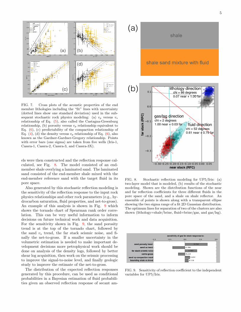
FIG. 7. Cross plots of the acoustic properties of the endmember lithologies including the “fit” lines with uncertainty(dotted lines show one standard deviation) used in the sub-sequent stochastic rock physics modeling: (a) vp versus vsrelationship of Eq. (5), also called the Castagna-Greenburgrelationship, (b) porosity versus vp relationship equivalent toEq. (6), (c) predictability of the compaction relationship ofEq. (4), (d) the density versus vp relationship of Eq. (6), alsoknown as the Gardner-Gardner-Gregory relationship. Pointswith error bars (one sigma) are taken from five wells (Iris-1,Cassra-1, Cassra-2, Cassra-3, and Cassra-3X).

els were then constructed and the reflection response cal-culated, see Fig. 8. The model consisted of an end-member shale overlying a laminated sand. The laminatedsand consisted of the end-member shale mixed with theend-member reference sand with the target fluid in itspore space.

Also generated by this stochastic reflection modeling isthe sensitivity of the reflection response to the input rockphysics relationships and other rock parameters (e.g., hy-drocarbon saturation, fluid properties, and net-to-gross).An example of this analysis is shown in Fig. 9 whichshows the tornado chart of Spearman rank order corre-lation. This can be very useful information to informdecisions on future technical work and data acquisition.For the sensitivity shown in Fig. 9, the sand porositytrend is at the top of the tornado chart, followed bythe sand vs trend, the far stack seismic noise, and fi-nally the net-to-gross. If a smaller uncertainty in thevolumetric estimation is needed to make important de-velopment decisions more petrophysical work should bedone on analysis of the density logs, followed by bettershear log acquisition, then work on the seismic processingto improve the signal-to-noise level, and finally geologicstudy to improve the estimate of the net-to-gross.

The distribution of the expected reflection responsesgenerated by this procedure, can be used as conditionalprobabilities in a Bayesian estimation of fluid probabili-ties given an observed reflection response of secant am-

FIG. 8. Stochastic reflection modeling for UP5/Iris: (a)two-layer model that is modeled, (b) results of the stochasticmodeling. Shown are the distribution functions of the nearand far reflection coefficients for three different fluids in thepore space of the sand, and a shale on shale reflector. Anensemble of points is shown along with a transparent ellipseshowing the two sigma range of a fit 2D Gaussian distribution.The optimum lines for separation of two of the clusters are alsoshown (lithology=shale/brine, fluid=brine/gas, and gas/lsg).

FIG. 9. Sensitivity of reflection coefficient to the independentvariables for UP5/Iris.

6

classj \ classi shale brine lsg gas

shale 96 4 0 0

brine 4 96 0 0

lsg 0 2 62 36

gas 0 0 30 70

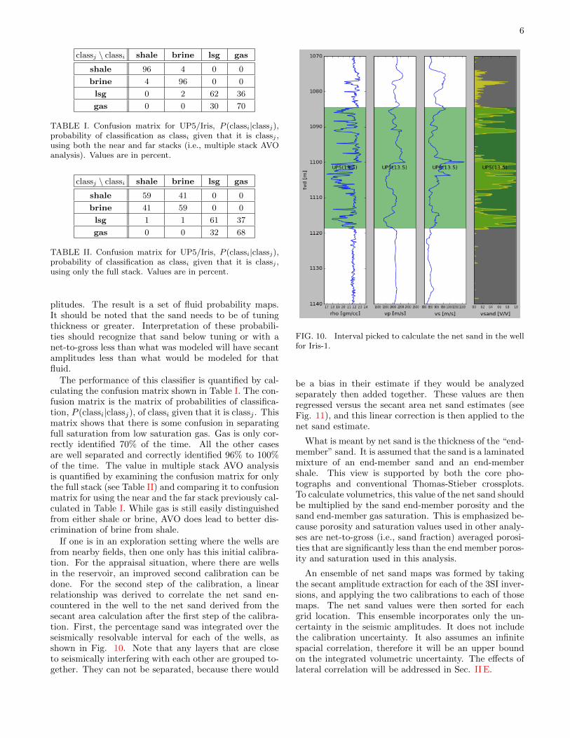
TABLE I. Confusion matrix for UP5/Iris, P (classi|classj),probability of classification as classi given that it is classj ,using both the near and far stacks (i.e., multiple stack AVOanalysis). Values are in percent.

classj \ classi shale brine lsg gas

shale 59 41 0 0

brine 41 59 0 0

lsg 1 1 61 37

gas 0 0 32 68

TABLE II. Confusion matrix for UP5/Iris, P (classi|classj),probability of classification as classi given that it is classj ,using only the full stack. Values are in percent.

plitudes. The result is a set of fluid probability maps.It should be noted that the sand needs to be of tuningthickness or greater. Interpretation of these probabili-ties should recognize that sand below tuning or with anet-to-gross less than what was modeled will have secantamplitudes less than what would be modeled for thatfluid.

The performance of this classifier is quantified by cal-culating the confusion matrix shown in Table I. The con-fusion matrix is the matrix of probabilities of classifica-tion, P (classi|classj), of classi given that it is classj . Thismatrix shows that there is some confusion in separatingfull saturation from low saturation gas. Gas is only cor-rectly identified 70% of the time. All the other casesare well separated and correctly identified 96% to 100%of the time. The value in multiple stack AVO analysisis quantified by examining the confusion matrix for onlythe full stack (see Table II) and comparing it to confusionmatrix for using the near and the far stack previously cal-culated in Table I. While gas is still easily distinguishedfrom either shale or brine, AVO does lead to better dis-crimination of brine from shale.

If one is in an exploration setting where the wells arefrom nearby fields, then one only has this initial calibra-tion. For the appraisal situation, where there are wellsin the reservoir, an improved second calibration can bedone. For the second step of the calibration, a linearrelationship was derived to correlate the net sand en-countered in the well to the net sand derived from thesecant area calculation after the first step of the calibra-tion. First, the percentage sand was integrated over theseismically resolvable interval for each of the wells, asshown in Fig. 10. Note that any layers that are closeto seismically interfering with each other are grouped to-gether. They can not be separated, because there would

FIG. 10. Interval picked to calculate the net sand in the wellfor Iris-1.

be a bias in their estimate if they would be analyzedseparately then added together. These values are thenregressed versus the secant area net sand estimates (seeFig. 11), and this linear correction is then applied to thenet sand estimate.

What is meant by net sand is the thickness of the “end-member” sand. It is assumed that the sand is a laminatedmixture of an end-member sand and an end-membershale. This view is supported by both the core pho-tographs and conventional Thomas-Stieber crossplots.To calculate volumetrics, this value of the net sand shouldbe multiplied by the sand end-member porosity and thesand end-member gas saturation. This is emphasized be-cause porosity and saturation values used in other analy-ses are net-to-gross (i.e., sand fraction) averaged porosi-ties that are significantly less than the end member poros-ity and saturation used in this analysis.

An ensemble of net sand maps was formed by takingthe secant amplitude extraction for each of the 3SI inver-sions, and applying the two calibrations to each of thosemaps. The net sand values were then sorted for eachgrid location. This ensemble incorporates only the un-certainty in the seismic amplitudes. It does not includethe calibration uncertainty. It also assumes an infinitespacial correlation, therefore it will be an upper boundon the integrated volumetric uncertainty. The effects oflateral correlation will be addressed in Sec. II E.

7

FIG. 11. Regression of the well net sand values versus thevalues estimated by the secant area after the first preliminarycalibration for UP5/Iris. OLS = Ordinary Least Squares fit.WLS = Weighted Least Squares fit. Dotted lines show onestandard deviation.

E. Building in lateral correlation

It is important to build in the lateral correlation intothe net sand ensemble before integrating the maps to ob-tain volumes. The reason is that the standard deviationof the volumes will be reduced by a factor R/

√Am due

to the lateral correlation, and be further reduced by afactor of

√1−NR2/Am due to the well control and lat-

eral correlation; where R is the variogram range, Am isthe area of the map, and N is the number of wells.

Lateral correlation and well values are built into theensemble of net sand maps using the method of Gun-ning, Glinsky, and White 8 . Input to this method is amost likely net sand map, a standard deviation map,the variogram, along with the net sand encountered ateach well location. Output from the analysis are up-dated most likely and standard deviation maps, alongan ensemble of correlated maps honoring the well con-trol. The anisotropic variogram is estimated by standardsemivariogram analysis (on the most likely net sand map)as shown in Fig. 12. The well control comes from thewell net sand points calculated from Fig. 10. The inputmost likely net sand map is just the most likely doublycalibrated net sand map using the most likely wavelet toinvert the unperturbed seismic data. The standard devi-ation map is calculated two different ways. The first is astandard deviation map of the ensemble of maps calcu-lated in Sec. II D. This is characteristic of the error in theseismic data and wavelet. The second is a standard de-viation map based on the error of the calibration shownin Fig. 11, truncated so that the range does not includenegative values of net sand. This will be characteristic ofthe calibration error.

The volumetric distribution is calculated by taking a

FIG. 12. Semivariogram analysis for UP5/Iris: (a) the fitvariogram with anisotropy, (b) semivariogram analysis for theanisotropy.

random map from the ensemble of correlated net sandmaps using the seismic standard deviation, then integrat-ing it over an area given by one of three contours chosenat random according to a probability of 20% for the con-tour of smallest and largest area, and 60% for the remain-ing contour. This makes the contours the P10, P50, andP90 contours. Porosity, gas saturation, gas expansionfactor, rock volume norm (determined by the distribu-tion of net sand volume from the ensemble of correlatednet sand maps using the calibration standard deviation),and a non-pay discount factor (used to compensate forlow saturation gas that is non-pay, but still produces anamplitude response) are chosen from suitably truncatednormal distributions. A Gas Initially In Place (GIIP)volume is calculated from these values. An accounting ofhow much of this volume comes from each of the field ar-eas is also done. This process is repeated as many timesas necessary to form a statistically significant ensembleof GIIP.

A sensitivity analysis is done on the total GIIP toeach of these factors. Again, this sensitivity analysis isvery valuable when it comes to making decisions aboutwhether to drill additional wells, and where the wells

8

should be located. Specific examples of the Value Of In-formation (VOI) decisions based on this sensitivity anal-ysis will be discussed in Sec. III.

III. RESULTS

The integrated analysis presented in Sec. II is appliedto the Cassra/Iris field offshore Trinidad. This is a gasfield with six wells that were provided for this study – twotargeting the UP5 interval, and four that targeted pri-marily the M0 interval. The quality of the well logs var-ied depending on their age. Many of the wells had shearlogs, but unfortunately most of the shear logs failed inthese unconsolidated sections due to fundamental flawsin the shear logging tool design. A well processed 3Dseismic survey which had Bandwidth Extension9 appliedto it was available. Only the full stack was used in thisanalysis. It can be seen in Fig. 8 that there would belittle value in a multiple stack AVO analysis for volumet-ric analysis. This was further quantified by examiningthe confusion matrix for only the full stack and compar-ing it to confusion matrix for using the near and the farstack in Sec. II C. There was little change in this matrixwhen the near and far stacks were used with respect todiscriminating gas from either brine or shale.

First, the two wells with the best logs, including a shearsonic (Cassra-1 and Iris-1) were used to do a waveletderivation as described in Sec. II A, followed by thestochastic sparse spike inversion described in Sec. II Bthat generated 100 realizations. The results are shown inFigs. 13, 14, 15, and 16. There is very good agreementbetween the well log and the result of the sparse spike in-version shown in Fig. 13. This agreement is significantlybetter than the original seismic runsum data. The noiselevel was improved from 1.4% to 1.0% in percent reflectiv-ity units. This should be compared to the 8.0% to 12.0%reflectivity of the the main target reflectors. This is verygood data. This improvement is further quantified byFig. 15 which shows the spectral signal-to-noise (SNR)before and after the SSI. Note that the useful bandwidthwas increased from 10-45 Hz to 5-95 Hz by the SSI. Itshould be noted that this large improvement would nothave been possible if it was not for the Bandwidth Ex-tension. The Bandwidth Extension needed the SSI, inorder to reach its full potential, because of the low fre-quency and ringy (i.e., many side lobes) wavelet that itleaves on the data (see Fig. 14). The SSI removes thiswavelet from the data. Figure 14 also shows the time-to-depth mapping with uncertainty that is output from thewavelet derivation. Note the correspondence to the soniclog, even though there is no explicit constraint to it. Fi-nally a key cross section through the SSI is shown in Fig.16. This shows very fine fault and stratigraphic detail.Of particular note is the classic off-lapping clinoforms ofthe M0 deltaic sequence.

Stratigraphic interval specific work was done. This pa-per presents the results for the UP5 turbidite sequence

FIG. 13. Comparison of the well acoustic impedance (red)to the seismic runsum (blue) and the sparse spike inversionimpedance (green) for the Cassra-1 and Iris-1 wells.

FIG. 14. (a) Ensemble of wavelets demonstrating the un-certainty in the wavelet. (b) Time-to-depth mapping withuncertainty shown as interval velocity compared to the sonicwell log for Cassra-1.

of the Iris reservoir. As described in Sec. II, a Stochas-tic Sparse Spike Inversion (3SI) was done based on thewavelet derivation, then an ensemble of secant amplitudeand area maps were extracted from the ensemble of 3SIacoustic impedance volumes. The most likely, calibratedamplitude map is shown in Fig. 17. This was used alongwith the conditional probabilities, shown in Fig. 8, togenerate the fluid probability maps, shown in Fig. 18.

It should be noted that the sand needs to be of tuningthickness or greater. Interpretation of these probabili-ties should recognize that sand below tuning or with anet-to-gross less than what was modeled will have secantamplitudes less than what would be modeled for that

9

FIG. 15. Spectral signal-to-noise-ratio (SNR) for the origi-nal Bandwidth Enhanced data, compared to the result of thesparse spike inversion.

FIG. 16. Representative cross section of the sparse spikeinversion impedance volume.

fluid.

Some comment should be made on the rock physicsrelationships that were used in the first part of the netsand calibration. Because many of the sands and shalespicked were not strict end members, the fit of the averagewas not representative of the end member (see Fig. 7).To correct for this, the edge of the cluster of points wasestimated and the orientation of the cluster determined.The trend that was used represented the edge of the clus-ter, had the orientation of the cluster of points, and hada reduced standard deviation. For the cases where therewere not enough points to determine the orientation ofthe cluster, the orientation of global reference trends wereused.

Then, the secant amplitude ensemble was two step cal-ibrated, laterally correlated, and tied to the wells to givethe mean and standard deviation net sand maps shownin Fig. 19. Preliminary evaluation of the volumetric dis-

FIG. 17. Secant amplitude extraction from the UP5. Unitsare reflection coefficient.

FIG. 18. Fluid probability maps for the UP5: (a) shale, (b)low saturation gas, (c) brine, (d) gas. Note that the probabil-ity of low saturation gas is overestimated and the probabilitygas is underestimated, especially in the dim zone shown inFig. 22, due to the effects described in Sec. II D.

10

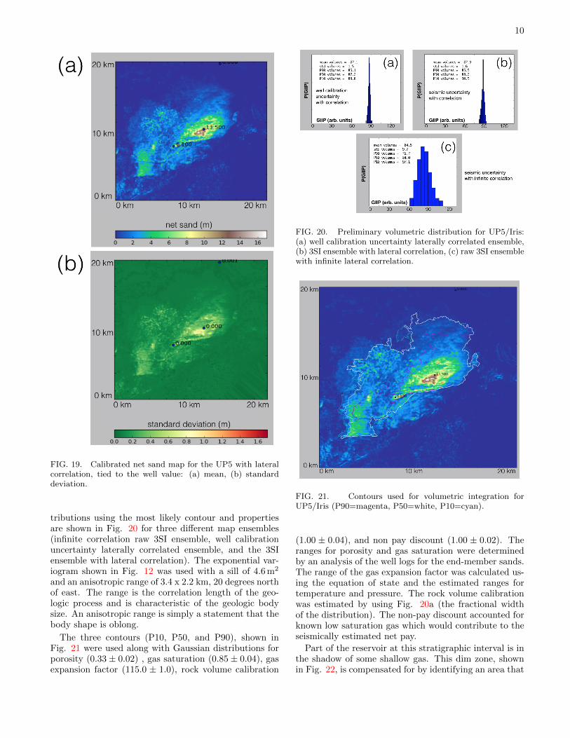
FIG. 19. Calibrated net sand map for the UP5 with lateralcorrelation, tied to the well value: (a) mean, (b) standarddeviation.

tributions using the most likely contour and propertiesare shown in Fig. 20 for three different map ensembles(infinite correlation raw 3SI ensemble, well calibrationuncertainty laterally correlated ensemble, and the 3SIensemble with lateral correlation). The exponential var-iogram shown in Fig. 12 was used with a sill of 4.6 m2

and an anisotropic range of 3.4 x 2.2 km, 20 degrees northof east. The range is the correlation length of the geo-logic process and is characteristic of the geologic bodysize. An anisotropic range is simply a statement that thebody shape is oblong.

The three contours (P10, P50, and P90), shown inFig. 21 were used along with Gaussian distributions forporosity (0.33 ± 0.02) , gas saturation (0.85 ± 0.04), gasexpansion factor (115.0 ± 1.0), rock volume calibration

FIG. 20. Preliminary volumetric distribution for UP5/Iris:(a) well calibration uncertainty laterally correlated ensemble,(b) 3SI ensemble with lateral correlation, (c) raw 3SI ensemblewith infinite lateral correlation.

FIG. 21. Contours used for volumetric integration forUP5/Iris (P90=magenta, P50=white, P10=cyan).

(1.00 ± 0.04), and non pay discount (1.00 ± 0.02). Theranges for porosity and gas saturation were determinedby an analysis of the well logs for the end-member sands.The range of the gas expansion factor was calculated us-ing the equation of state and the estimated ranges fortemperature and pressure. The rock volume calibrationwas estimated by using Fig. 20a (the fractional widthof the distribution). The non-pay discount accounted forknown low saturation gas which would contribute to theseismically estimated net pay.

Part of the reservoir at this stratigraphic interval is inthe shadow of some shallow gas. This dim zone, shownin Fig. 22, is compensated for by identifying an area that

11

FIG. 22. Contour used to define the dim zone in the UP5:(a) extent of the shadowed area on the net sand map, (b) areaof un-shadowed amplitude shown on the reflection coefficientmap, (c) area of shadowed amplitude shown on the reflectioncoefficient map. Amplitude ratio is 0.153/0.063 = 2.4.

FIG. 23. Integrated volumetric distributions for UP5/Iris.The dark, blocky, line is the blocked distribution function.The smooth, transparently shaded curve is a fit Gaussian dis-tribution.

is not shadowed and a stratigraphically similar area thatis shadowed. The difference in the mean amplitudes ofthese areas is calculated and the volume of the area ofthe dim zone is multiplied by this factor.

The resulting volumetric distributions (with 3000 re-alizations) that combine all these factors are shown inFig. 23. Note that this distribution is multimodal. Thedifference between these two modes is the area betweenthe P50 and the P90 contours. The results of these vol-umetrics are shown in Table III.

The sensitivity of the Iris volumes is shown in Fig.24. This is an important figure that warrants some fur-ther discussion. The dominate input uncertainties arethe choice of contour, sand porosity, gas saturation, andthe net sand calibration (in that order). A well into thearea between the P50 and P90 contour that was never

unit mean std dev P90 P50 P10

Iris(total) 89.2 16.2 60.8 93.6 105.5

Iris (uncorrected) 81.7 15.0 55.8 85.6 97.2

dim zone 7.5 1.4 5.1 7.9 9.1

Iris (P50 contour) 95.6 8.0 85.5 95.2 106.3

TABLE III. Volumetric distributions of the UP5 reservoir in-terval. Units are arbitrary. Dim zone volume is the additionalvolume added by the correction.

FIG. 24. Sensitivity analysis, shown as tornado chart, of theUP5/Iris GIIP to the independent stochastic variables.

penetrated would be the best way to reduce the domi-nate uncertainty in the choice of contour. Next a morecareful petrophysical analysis could be done to determinethe range of the porosity and gas saturation of the endmember sand. Finally, an additional well could be drilledin the thickest part of the reservoir to improve the cali-bration of the net sand maps.

IV. CONCLUSIONS

A state-of-the-art stochastic wavelet derivation was ap-plied, giving the seismic noise level, time-to-depth map-pings, and the wavelet – all with uncertainty. This wasused to do a novel stochastic sparse spike inversion. Anensemble of secant area maps were extracted from theensemble of sparse spike inversion impedance volumes.The secant area maps were calibrated to net sand mapsin a two step process. Lateral correlation was added tothis ensemble of net sand maps and they were tied tothe well values of net sand. Finally, uncertainty in thecontour area, gas saturation, porosity, and gas expansionfactor were added to give an integrated view of the vol-umetric uncertainty. A sensitivity analysis was done togive insight into the value of information – what datashould be acquired and what wells should be drilled inorder to maximize the return on capital investment.

ACKNOWLEDGMENTS

The authors would like to thank Centrica E&P for sup-porting this work, supplying the Cassra/Iris Field data,and granting permission to publish. The contributionsof Petrotrin, as the joint venture partner, and the Min-istry of Energy and Extractive Industries (MEEI) are

12

recognized and appreciated. We would also like to thankGeotrace Technologies for their financial support, and in-tellectual encouragement.

1J. Gunning and M. E. Glinsky, Computers & Geosciences 32, 681(2006).

2M. E. Glinsky, “Bayesian seismic wavelet extraction,” (HoustonGeophysical Society, Houston, TX, 2006) Feb, 2006.

3C. Dossal and S. Mallat, “Sparse spike deconvolution with mini-mum scale: Proceedings of signal processing with adaptive sparsestructured representations, 123–126,” (2005).

4I. Daubechies, M. Defrise, and C. De Mol, Communications onPure and Applied Mathematics 57, 1413 (2004).

5M. Glinsky, J. Kalifa, and S. Mallat, “Method for determiningimpedance coefficients of a seismic trace,” (2009), a US Patent7,519,477.

6G. Gardner, L. Gardner, and A. Gregory, Geophysics 39, 770(1974).

7J. P. Castagna, H. W. Swan, and D. J. Foster, Geophysics 63,948 (1998).

8J. Gunning, M. E. Glinsky, and C. White, Computers & Geo-sciences 33, 630 (2007).

9M. Smith, in 11th International Congress of the Brazilian Geo-physical Society (2009).