
Methods to Generate the Yearly Shutdown- Schedule of a...
82
Methods to Generate the Yearly Shutdown- Schedule of a Basic Oxygen Steel Plant Master Assignment Industrial Engineering and Management by Michiel Bel
-
Upload
truongcong -
Category
Documents
-
view
216 -
download
0
Transcript of Methods to Generate the Yearly Shutdown- Schedule of a...

Methods to Generate the Yearly Shutdown-Schedule of a Basic Oxygen Steel Plant
Master Assignment Industrial Engineering and Management by Michiel Bel

Methods to Generate the Yearly Shutdown-Schedule of a Basic Oxygen Steel Plant
1
Date and Place: August 2013, Velsen-Noord Author: Michiel Bel Supervisors: Dr. Ir. J.M.J. Schutten, Universiteit Twente Dr. Ir. M.R.K. Mes, Universiteit Twente R. Broers, Tata Steel Commissioned by: Tata Steel’s Basic Oxygen Steel Plant 2

Methods to Generate the Yearly Shutdown-Schedule of a Basic Oxygen Steel Plant
2
Management Summary Tata Steel’s Basic Oxygen Steel Plant in IJmuiden converts pig iron into sheets of steel, which requires
several installations. These installations all require different maintenance jobs, which are specified in
the SAP system where the job’s cycle time, duration, priority, start date, etc. are stored. Currently,
Tata Steel bases the Yearly Shutdown-Schedule (YSS) too much on the maintenance needs of
installations, instead of on the jobs that have to be performed on these installations. Furthermore,
Tata Steel generates the YSS based on manual processes, without a formal methodology. Hence, the
research question of this research is:
Method In the literature, our problem is called the ‘Maintenance Scheduling Problem’ (MSP) and the problem
is solved in the literature by applying a local search heuristic, because the problem is too complex to
be solved to optimality. Our MSP is even more complex, mainly due to the high amount of possible
routes through the Basic Oxygen Steel Plant. In order to create a transparent and subjective method
to generate a YSS, we formulated the MSP as a Mixed-Integer Program, which includes the
restrictions on shutting down an installation. The method contains four ranked objectives, in which a
lower ranked objective can never by improved at the cost of a higher ranked objective:
1. Minimize the overflow of pig iron (deregulating the Blast-Furnaces and dumping at Harsco).
2. Minimize working in overtime (during the weekends and on working days before 7am and
after 3pm).
3. Minimize deviating from the job’s cycle time.
4. Maximize the spreading of jobs.
In order to solve the MSP, we applied a Simulated Annealing (SA) heuristic that uses four runs to
subsequently optimize each objective.
Results The analysis of the results of our four-run SA approach clearly shows the correctness of the approach
with respect to clustering jobs in order to minimize the overflow: our approach causes a decrease in
the objective value of 89% with respect to the initial schedule, as Table 1 shows. In Table 1, the
‘initial’ column shows the values of the four objectives if every job is scheduled at its start date in
SAP.
Table 1 - Results of our SA approach
Initial After SA Decrease
Objective 653,066.4 74,291 -89%
Overflow 651,066.4 72,067 -89%
Overtime 2,000 2,155 +8 %
Deviation (/1000) 0 69,662 - %
Spread (/1000) 5.03 4.149 -18%
How can the current method of developing the yearly shutdown-schedule at the Basic Oxygen
Steel Plant of Tata Steel be improved, such that the restrictions are met and are clear, and that all
iron produced by the Blast-Furnaces is processed?

Methods to Generate the Yearly Shutdown-Schedule of a Basic Oxygen Steel Plant
3
Additionally, we applied two Iterative Improvement approaches, a one-run SA approach, and a
combined approach to the same MSP. From this analysis, we conclude that both our four-run SA and
the one-run SA outperform the Iterative Improvement approaches and the combined approach.
Although it did not out- or underperform the method in the small experiment that we performed, we
expect our four-run SA approach to outperform the one-run SA approach on the long run, because
the one-run SA approach finds a bad local optimum relatively quickly.
Furthermore, the analysis shows that not all rules of thumb that Tata Steel currently applies to
generate the YSS remain valid from an overflow point of view, whereas we are unable to conclude on
the validity of the rules of thumb from any other point of view, such as safety. Although not all of
these rules of thumb remain valid, the current YSS seems to outperform our YSS. However, 55% of
the jobs do not fit to the shutdowns in the YSS as Tata Steel generated it. This is mainly due to our
usage of tight bounds on the allowed deviation from the cycle time: we expect that our approach
outperforms the current manual approach if it is based on the same restrictions.
Conclusions and Recommendations As mentioned in the previous section, the currently applied restrictions differ from the restrictions as
we applied them, which is mainly due to the incorrectness or unavailability of the job’s duration, the
priority, and cycle time. We propose determining the correct parameters for every job in SAP, such
that the YSS is based on these data, which improves the objectivity of the restrictions and the trust in
the output. Furthermore, we recommend clustering jobs in order to decrease the runtime of the SA
approach. Especially clustering the jobs on the casting installations decreases the problem size
without decreasing the quality of the method and the YSS.
Finally, the main advantages of our method over the current method to generate the YSS are mainly
due to the scheduling of jobs instead of installations (as Tata Steel currently does) and due to the
computerized approach instead of a manual approach. The main advantages are:
Sections have more insight in and a better overview of the maintenance to perform during
the year.
The method to generate the YSS is neither based on experience, nor a manual process.
Less additional maintenance jobs appear during the year, because the schedule includes
every job. This leads to less rescheduling and more time to prepare a shutdown.
The method takes four objectives into account for each and every job.
The consequences of rescheduling can be analyzed quickly and comprehensively.
The restrictions of the YSS are clear. Hence, the reasoning behind the scheduling itself is
clear.

Methods to Generate the Yearly Shutdown-Schedule of a Basic Oxygen Steel Plant
4
Preface By means of this report, I finish my master Industrial Engineering and Management at the University
of Twente. This report contains my research towards an improved method to generate the yearly
shutdown-schedule at the Basic Oxygen Steel Plant of Tata Steel IJmuiden. This master assignment
offered me the opportunity to work on both maintenance concepts and complex schedules within a
plant with an impressive production process, which is part of a chain of complex and interesting
processes at the Tata Steel IJmuiden site.
For providing me this opportunity, the offered supervision, and shown interest from the initial
contact until handing in this report, I would like to thank Tata Steel. I would especially thank my Tata
Steel-supervisor Randy Broers for providing me with useful feedback and introducing me in a
complex plant and system. I enjoyed using the workplace next to you.
Furthermore, I would like to thank Marco Schutten and Martijn Mes, my supervisors from the
University of Twente. The useful feedback that I received while carrying out my research was full of
clear content and often helped me obtaining new insights in my research. Especially the different and
complementary types of feedback helped me obtaining these.
I would like to thank my parents for their interest in this assignment and for their financial support
during my studies. Finally, I would like to thank Sandra for moving to Enschede during her studies, to
join me during my years in Enschede.
Michiel Bel

Methods to Generate the Yearly Shutdown-Schedule of a Basic Oxygen Steel Plant
5
Table of Contents 1. Introduction ..................................................................................................................................... 6
1.1 Background and Motive .......................................................................................................... 6
1.2 Core Problem and Research Questions ................................................................................... 8
1.3 Approach and Outline ........................................................................................................... 10
2. Current Situation ........................................................................................................................... 11
2.1 Flows through the Plant ........................................................................................................ 12
2.2 Process of Generating and Applying the Yearly Shutdown-Schedule ................................... 15
2.3 Complications ........................................................................................................................ 17
2.4 Cycle Time Defined ................................................................................................................ 19
2.5 Restrictions to Scheduling Maintenance ............................................................................... 20
3. Literature Review .......................................................................................................................... 23
3.1 Position in the Literature ....................................................................................................... 23
3.2 Approaches to Comparable Problems ................................................................................... 26
3.3 Options to Improve the Process ............................................................................................ 26
3.4 Concluding Remarks .............................................................................................................. 31
4. Model of the Maintenance Scheduling Problem at Tata Steel ..................................................... 32
4.1 Evaluation of the Modeling Techniques ................................................................................ 32
4.2 Mathematical Model of the Maintenance Scheduling Problem ........................................... 32
4.3 Implementing the Local Search Technique ........................................................................... 38
4.4 Concluding Remarks .............................................................................................................. 44
5. Analysis and Discussion of the Results .......................................................................................... 45
5.1 Initial Solution........................................................................................................................ 45
5.2 Performance of Simulated Annealing ................................................................................... 45
5.3 The Generated YSS ................................................................................................................ 56
5.4 Computation Time ................................................................................................................. 63
5.5 Summarizing the Results ....................................................................................................... 65
6. Conclusions and Recommendations ............................................................................................. 66
6.1 Conclusions ............................................................................................................................ 66
6.2 Further Research ................................................................................................................... 69
Bibliography ........................................................................................................................................... 72
Appendices ............................................................................................................................................ 77
A Translation of Terms .................................................................................................................. 77
B Maps the Basic Oxygen Steel Plant and the IJmuiden Site........................................................ 79
C Defining the Minimum and Maximum Differences between Neighboring Solutions .............. 81

Methods to Generate the Yearly Shutdown-Schedule of a Basic Oxygen Steel Plant
6
1. Introduction This research focusses on the scheduling of installation shutdowns to perform maintenance at Tata
Steel’s Basic Oxygen Steel Plant 21 in IJmuiden. Figure 1 shows a part of the Tata Steel IJmuiden site,
and Appendix B contains a map of both the IJmuiden site and the Basic Oxygen Steel Plant. Tata Steel
IJmuiden employs approximately 9,000 people, of which 1,000 are employed by the Basic Oxygen
Steel Plant. The Basic Oxygen Steel Plant converts liquid iron – produced by two blast furnaces – into
sheets of steel, which are further processed by the Direct Sheet Plant and the Hot Strip Mill. Section
1.1 explains the motive and importance of this research for both Tata Steel and the scientific
research; Section 1.2 derives the research question and this chapter finishes with the outline of this
research in Section 1.3.
1.1 Background and Motive Every manufacturing organization faces the breakdowns of machines at unexpected and unwanted
moments. All these organizations use some kind of approach to perform maintenance, based on the
balance between costs, time, and safety. Maintenance is often seen as a cost function only, instead
of a way to save money and time during breakdowns and for a company such as Tata Steel – with a
continuous process and expensive installations – the call for maintenance often comes at an
inopportune moment. Still, maintenance is more and more accepted as needed to increase the total
amount of output and the output’s quality, and Tata Steel recognizes that the planning of
maintenance should be improved. Figure 2 shows a simplified flowchart of the continuous process, in
which some installations are more critical to the flow than other installations. Currently, the yearly
process of planning the shutdown of an installation aims to attain a high flow through the plant, by
scheduling the shutdowns of these installations in a finely tuned way. Note that we add more
installations to this flow in Chapter 2.
1 Appendix A contains a translation of several terms from English to Dutch
Figure 1 - A view over a part of the IJmuiden Tata Steel Site

Methods to Generate the Yearly Shutdown-Schedule of a Basic Oxygen Steel Plant
7
The relevance of this research for Tata Steel is especially in acquiring new insights in maintenance
scheduling as well as in a method to schedule maintenance. This research is also relevant to other
organizations, because every organization with a continuous process that does not have the
possibility to change the flow of goods via spare machines needs to cut the flow by shutdowns, in
order to maintain the installations. All these organizations can use new insights in the process and
methods of developing a shutdown schedule. Next to the relevance to organizations, this research’s
relevance to science lies in the fact that maintenance scheduling is mostly researched in the power
generating industry, where simpler flows are considered. Dekker (1996) recognizes an increasing
trend from the late 1980s to the early 1990s of research in the field of maintenance optimization and
since that time, more and more literature has become available on the maintenance scheduling
topic, although its focus remains on the power generating industry. Furthermore, the relevance to
science lies in the fact that maintenance scheduling is not highlighted in basic scheduling books, such
as Pinedo (2009), while there is a clear link between maintenance and scheduling. He does discuss
the differences between manufacturing and service industries and from that discussion we conclude
that maintenance is somewhere in between these two types of industries and should be dealt with
on the interface of manufacturing and services, making maintenance planning and scheduling an
even more interesting topic. So, maintenance becomes an important research topic in the scientific
literature, and Tata Steel improves its maintenance policy and process, to attain high uptime and
more output.
Figure 2 - Simplified flowchart of the process from the Blast Furnaces via the Basic Oxygen Steel Plant to the Direct Sheet Plant and the Slab Yard
Methods to Generate the Yearly Shutdown-Schedule of a Basic Oxygen Steel Plant
8
1.2 Core Problem and Research Questions To perform planned maintenance at the Basic Oxygen Steel Plant, several installations need to be
taken out of service. Every installation has several maintenance jobs attached to it (lubricating,
replacement of parts, etc.) and these jobs all have a cycle time2, which is defined by a maintenance
engineer. These cycle times are combined to schedule the shutdown of an installation and these
shutdowns are combined to a yearly shutdown-schedule (YSS), which shows the moments of a
shutdown.
The shutdown moments are set such that the flow through the plant is guaranteed and every
installation is maintained. Actually, the most important aim is to guarantee a flow through the plant
that is high enough to process the pig iron processed by the Blast-Furnaces. The scheduling is based
on human knowledge about restrictions with respect to taking different installations together out of
service and these are not clear to everybody, such that convincing others about its correctness is
hard. Moreover, the scheduling is based on rules of thumb that have proven their usability in the
past, but it is unclear whether each of these rules is needed to set up the schedule. Still, most of
these rules are based on cycle times through the plant. The scheduling process of setting up a
shutdown schedule for the installations in the Basic Oxygen Steel Plant repeats itself every year and
the YSS needs to be revised several times before it is accepted and frozen. Another disadvantage of
the unclear process and the rescheduling before freezing the YSS, is the decreasing trust in the
developed YSS. Part of the process is the method of deducting the YSS from the different
maintenance needs, which currently holds that the different installation engineers define the
installation cycle time, without really basing this on the cycle times of maintenance jobs that are
stored in SAP. Therefore, this process is too much based on experience and human knowledge. That
is why Tata Steel recognizes a possibility to increase the clarity and understandability of the YSS.
Finally, because of the manual approach to define and combine the cycle times of installations, we
question the correctness of the resulting schedule.
So far, we have mentioned several problems in the current process of generating the YSS: the
process is based on human knowledge, the method is based on a manual approach, the process is
unclear and incomprehensible, rescheduling is required, and the outcome has a questionable quality.
While the process basically covers three steps – the determination of the cycle times, the generation
of the schedule, and the implementation of the schedule – we only focus on the generation itself,
because most problems appear there (rules of thumb, outcome, manual approach). Although the
focus is on the method to generate the schedule, we do recognize the importance of the other two
steps. Now, the main problem with respect to maintenance scheduling at the Basic Oxygen Steel
Plant is:
To improve the method, a manual process should be prevented, the trust and understandability
should be higher, and the outcome should not be questionable anymore. So, a model should be
developed that clarifies the restrictions, such that the trust in the correctness of the YSS increases.
2 The cycle time of maintenance is the time between two identical and subsequent maintenance jobs. In
practice, this time varies between two bounds (e.g., a cycle time of 10 weeks means that the job should be repeated after at least 9 and at most 11 weeks).
The current method of generating the yearly shutdown-schedule is unclear, does not lead to the best
schedule, and is too much based on human knowledge, manual processes, and rules of thumb.

Methods to Generate the Yearly Shutdown-Schedule of a Basic Oxygen Steel Plant
9
Hence, the model should have high face validity (or logical validity), which means that the process
seems logical. So, if the process is composed of understandable steps and restrictions, the YSS (the
result of the process) should be intuitively understandable. Notice that high face validity only means
that the process looks like it obtains good solutions, rather than that it finds good solutions. Recall
that we only focus on the method of generating a YSS, so we improve the method of generating a YSS
given the cycle times and maintenance needs of installations, while leaving out the process of
determining these values (e.g., determining the cycle times, determining the maintenance needs,
changing the way of approaching the YSS).
Furthermore, the main task of maintenance management is to guarantee availability (Moghaddam,
2008), which equals – for this research – guaranteeing the flow of steel through the plant or making
sure that all iron produced by the Blast-Furnaces, is processed by the Basic Oxygen Steel Plant. While
there are hardly any buffers in the plant, the iron is only processed if the cycle time through the
different areas of the plant is at most the Blast-Furnaces’ cycle time. Section 2.4 elaborates on this
topic. In addition to that main task of guaranteeing availability, maintenance management should
guarantee some repeatability and predictability of maintenance moments, such that scheduling is
possible and everybody expects the shutdown of an installation. So, in order to make sure that a new
method is accepted, the capacity of the Basic Oxygen Steel Plant should be high enough to process
the iron supplied by the Blast-Furnaces, while the maintenance cycles are repeating.
Both the problem and the explanation above lead to the following research question:
In order to answer this question, we first need to have a better insight in the current process of
developing the YSS, which results in the first sub-question:
1. How is the yearly shutdown-schedule currently developed at the Basic Oxygen Steel Plant?
a. What are the current steps to generate the YSS?
b. What are the restrictions of the YSS?
c. How should the cycle time be defined?
Based on the first question, we are able to position this research in the literature and we are able to
derive useful insights for this research from that literature. So, our second sub-question is:
2. How should this research be positioned in the literature?
a. How is the problem described in the literature?
b. What can we learn from the literature to improve the current method of scheduling
maintenance at the Basic Oxygen Steel Plant?
c. Which methods are applied in the literature?
How can the current method of developing the yearly shutdown-schedule at the Basic Oxygen
Steel Plant of Tata Steel be improved, such that the restrictions are met and are clear, and that all
iron produced by the Blast-Furnaces is processed?

Methods to Generate the Yearly Shutdown-Schedule of a Basic Oxygen Steel Plant
10
After answering these questions, we can develop a new method to generate the YSS:
3. What is the most suitable option to improve the current method of scheduling shutdowns,
taking into account the method’s clarity and understandability, such that the flow is
guaranteed and the restrictions are met?
a. What option discussed in the literature suits best to our problem?
b. How can we adapt that option to make it fit to our problem?
c. How should this option be implemented?
Finally, we have to reflect on the selected method and evaluate the results:
4. What are the results of applying the selected method?
a. What is the improvement in the flow?
b. What is the improvement in clarity and understandability?
c. How bad/well is the current method (i.e., are the rules of thumb useful)?
1.3 Approach and Outline In Chapter 2, we answer the first question by interviewing schedulers, by analyzing the map of the
plant, and by analyzing existing reports. Chapter 3 positions this research in the literature and
translates the literature to insights applicable to the current situation of the problem. Chapter 3 is
solely based on a literature review. Chapter 4 answers sub-question 3 based on both the literature
research in Chapter 3 and our own insights. Chapter 5 describes and discusses the results of
implementing the options chosen in Chapter 4. Chapter 6 contains our conclusions and
recommendations.
Methods to Generate the Yearly Shutdown-Schedule of a Basic Oxygen Steel Plant
11
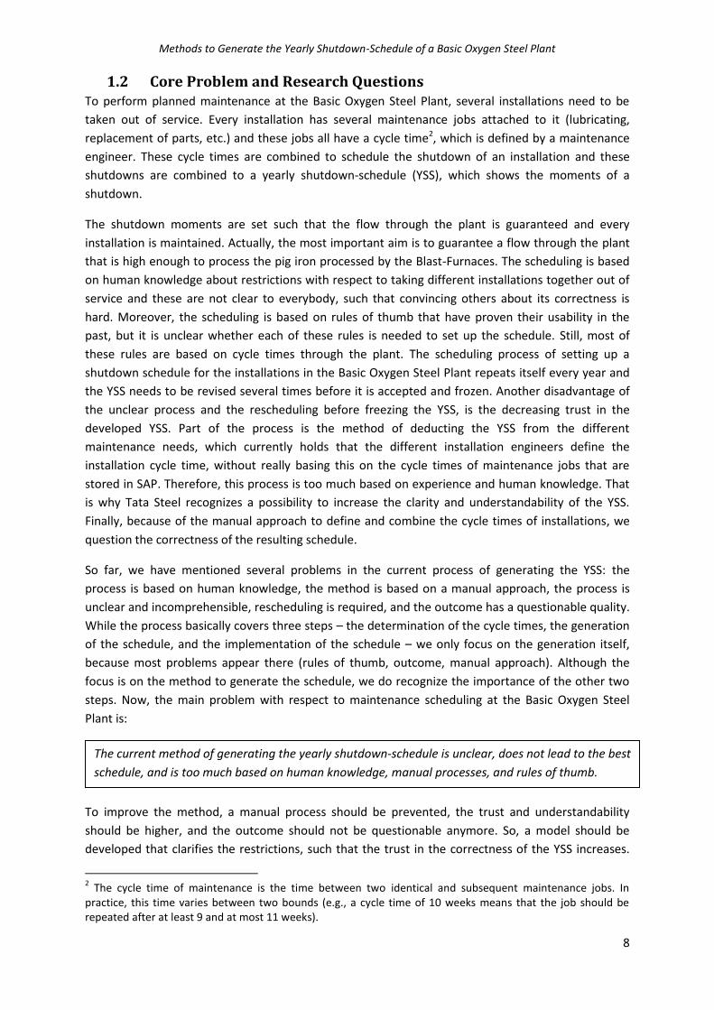
2. Current Situation This chapter explains the current situation – with respect to planned maintenance – at the Basic
Oxygen Steel Plant. This chapter comprises a part on the flows of steel through the plant and a part
on the developing of the yearly shutdown-schedule (YSS). We explain the current flow of iron, scrap,
steel, and slag through the Basic Oxygen Steel Plant in Section 2.1, before we explain the current
process of developing the YSS in Section 2.2. Section 2.3 explains the complications in the current
process, and Section 2.4 and Section 2.5 clarifies the terms: cycle time and restrictions.
Figure 3 - Simplified lay-out of the Basic Oxygen Steel Plant This figure shows the different installations we consider in this research. Every Transverse Transport contains one unit moving along the transport. The flow is as follows: liquid iron arrives at the Pits; there, the iron is tapped into a pig iron ladle and a Charging Crane moves the ladle to a Roza. From the Roza, the Charging Crane takes the ladle to a Converter,
where the scrap is added by a Charging Crane. The steel moves, via a Converter Transport and a Casting Crane, in a steel-ladle to one of the Ladle Furnaces, one of the Stirring Stations, or the RH-OB installation. Then it either moves to the Direct Sheet Plant (DSP), or via the Casting Installations, Gantry Cranes and the Slab Yard to the Hot Strip Mill (HSM).
Methods to Generate the Yearly Shutdown-Schedule of a Basic Oxygen Steel Plant
12
2.1 Flows through the Plant The Tata Steel IJmuiden site is made up of several separate plants that together manufacture sheets
and roles of steel (Appendix B.1 contains a map of the site). The relevant plants for this research are
the two Blast-Furnaces, (especially) the Basic Oxygen Steel Plant, and – although less relevant – the
Direct Sheet Plant and the Hot Strip Mill. The Blast-Furnaces produce pig iron (liquid iron), which is
transported by hot metal cars to the Basic Oxygen Steel Plant. As the name implies, this steel plant
converts the iron into steel: either sheets or roles. Finally, the sheets and roles are transported to the
Direct Sheet Plant (DSP) and the Hot Strip Mill respectively, where they are prepared for the
customer and further operations, such as galvanizing and cold rolling. This research’s focus is on the
maintenance scheduling of the Basic Oxygen Steel Plant, which is influenced by the supply of iron of
the predecessors (Blast-Furnaces) and the capacity and the demand for steel of the succeeding DSP,
because the DSP is directly attached to the Basic Oxygen Steel Plant, whereas the Hot Strip Mill has
the possibility to store the sheets of steel before handling these. The only way to buffer between the
Blast-Furnaces and the Basic Oxygen Steel Plant, is by means of filling the hot metal cars, but this
type of buffering is obviously limited.
Figure 3 contains a simplified map of the Basic Oxygen Steel Plant and only shows the installations
that we consider in this research. Recall that Appendix B.2 contains a more detailed map of the plant
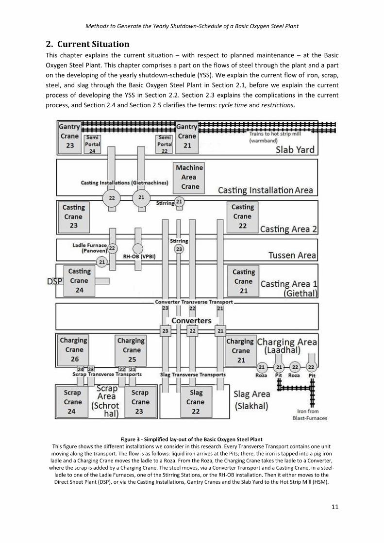
and that hot metal cars (Figure 4) transport pig iron to the pits. From Figure 3, we derive Figure 5
that contains the flows through the plant from the Blast-Furnaces, via the hot metal cars and the
Basic Oxygen Steel Plant to the DSP and train to the Hot Strip Mill. As mentioned before, the
shutdown of a Blast-Furnace means that the supply of pig iron decreases and installations are out of
supply. On the other hand, shutting down an installation while both Blast-Furnaces produce pig iron,
may lead to the need to deregulate the Blast-Furnaces to lower the amount of iron processed by the
Blast-Furnaces and so the amount of iron to be processed by the Basic Oxygen Steel Plant. Whether
or not deregulation of the Blast-Furnaces is required depends on the impact of shutting down that
installation on the capacity of the Basic Oxygen Steel Plant, because there may be the possibility to
use another flow (e.g., Converter 21 instead of Converter 22) and pig iron may be dumped and
reused as scrap. Figure 6 and Figure 7 show the charging of respectively pig iron and scrap into the
Converter by a Loading Crane.
Figure 4 – hot metal car, transports the pig iron from the Blast-Furnaces to the Basic Oxygen Steel Plant (RolandRail.net, 2005)

Methods to Generate the Yearly Shutdown-Schedule of a Basic Oxygen Steel Plant
13
Figure 5a - Flow through the Basic Oxygen Steel Plant
Slag
Are
aR
aw Ir
on
Des
ulp
hu
lizer
Inst
alla
tio
n (
Ro
za)
Ho
t m
etal
car
sSc
rap
Tra
nsv
erse
Tr
ansp
ort
Ch
argi
ng
Are
aSl
ag t
ran
sver
se
tran
spo
rtP
its
Sup
ply
fro
mB
last
-Fu
rnac
eC
on
vert
ers
Ch
argi
ng
Are
a
Pit
21
Pit
22
Ro
za 2
1
Ro
za 2
2
Co
nve
rter
21
Co
nve
rter
22
Co
nve
rter
23
Pig Iron
Pig Iron
Pig Iron
Ch
argi
ng
Cra
ne
21
Ch
argi
ng
Cra
ne
25
Pig Iron
Pig
Iron
Ch
argi
ng
Cra
ne
21
Ch
argi
ng
Cra
ne
25
Tran
sver
se
tran
spo
rt 2
1
Tran
sver
se
tran
spo
rt 2
2
Tran
sver
se
tran
spo
rt 2
3
Tran
sver
se
tran
spo
rt 2
4
Tran
sver
se
tran
spo
rt 2
1
Tran
sver
se
tran
spo
rt 2
2
Tran
sver
se
tran
spo
rt 2
3
Slag
Ch
argi
ng
Cra
ne
21
Ch
argi
ng
Cra
ne
25
Ch
argi
ng
Cra
ne
26
ScrapScrap
Cra
ne
Trai
n
Slag
Slag
SteelSteel
Slag
Ho
t m
etal
car
Ho
t m
etal
car
Ho
t m
etal
car
Ho
t m
etal
car
Pig Iron
Scra
p D
epo
tB
last
-Fu
rnac
e 7
Bla
st-F
urn
ace
6
Scra
pcr
ane
21
Scra
pcr
ane
22
Steel

Methods to Generate the Yearly Shutdown-Schedule of a Basic Oxygen Steel Plant
14
Cas
tin
gR
H-O
B In
stal
lati
on
Slag
Are
aSl
abtr
ack
Cas
tin
g Tr
ansv
erse
tr
ansp
ort
Cas
tin
g A
rea
Cas
tin
g A
rea
Slab
Are
a
Lad
le
Furn
ace
21
Lad
le
Furn
ace
22
Cas
tin
g In
stal
lati
on
2
1
Cas
tin
g In
stal
lati
on
2
2
Sem
i Po
rtal
C
ran
e 2
2
Sem
i Po
rtal
C
ran
e 2
4
Cas
tin
g C
ran
e 2
1
Cas
tin
g C
ran
e 2
4
Cas
tin
g C
ran
e 2
2
Cas
tin
g C
ran
e 2
3
Cas
tin
g A
rea
1
Cas
tin
g A
rea
2
RH
-OB
In
stal
lati
on
Stir
rin
g St
atio
n 2
3
Stir
rin
g St
atio
n 2
1
Cas
tin
g C
ran
e 2
1
Cas
tin
g C
ran
e 2
4
Cas
tin
g C
ran
e 2
2
Cas
tin
g C
ran
e 2
3
Gan
try
Cra
ne
21
Gan
try
Cra
ne
23
Cra
ne
Trai
n
Slag
Tran
sver
se
tran
spo
rt 2
1
Tran
sver
se
tran
spo
rt 2
2
Tran
sver
se
tran
spo
rt 2
3
SteelSteel
Dir
ect
Shee
t P
lan
t
Tran
spo
rt
Trai
n t
o H
ot
Stri
p M
ill
Trai
n t
o H
ot
Stri
p M
ill
Steel
Figure 5b - Flow through the Basic Oxygen Steel Plant

Methods to Generate the Yearly Shutdown-Schedule of a Basic Oxygen Steel Plant
15
Finally, a shutdown of one of the cranes pictured in Figure 3 may mean that an installation is locked
out of possible supply and may also lead to locking another crane. For example, the shutdown of
Charging Crane 25 in the Charging Area means that the crane is put as far as possible to the left side
of the picture. Now, Charging Crane 26 cannot be used because it is isolated and for the same reason
Scrap Transverse Transports 22, 23, and 24 cannot be used either. Consequently, Charging Crane 21
should take the pig iron ladle from the Pits to the Rozas and further to the Converters, but also put
scrap from Scrap Transverse Transport 21 into a converter, which obviously has its impact on the
cycle time in the Charging Area. In practice, some routes shown in the figure are not used for
practical reasons and we return to that point in Section 2.5. Notice that Figure 5 shows both the
Charging Area and the Casting Area two times, meaning that these cranes have more tasks. For
example, the Charging Cranes charge pig iron into the converters, but also charge scrap into the
same converter.
2.2 Process of Generating and Applying the Yearly Shutdown-Schedule In the current situation, Tata Steel develops the YSS for the next fiscal year (April to March) between
May and October and bases it solely on planned maintenance. The development can be divided into
four phases, which Figure 8 depicts. During Phase 1, the installation engineers belonging to the
section3 that manages the installation define the maintenance needs of the different installations
and store these needs and the corresponding cycle times in PO-plans4 in SAP. As a reminder for the
job, SAP shows a pop-up of the PO-plan a preset number of weeks before the maintenance has to be
performed.
3 The ‘Basic Oxygen Steel Plant 2’ is made up of 5 sections that are all responsible for a set of installations.
4 PO-plan stands for the Dutch term ‘periodiek onderhoud’-plan, which means ‘periodical maintenance’-plan,
and is a function in SAP. These plans are used to store maintenance jobs and its corresponding cycle times. PO-plans pop-up a preset number of weeks before the maintenance is actually performed.
Figure 6 - Charging of pig iron into a converter
Figure 7 - Charging of scrap into a converter

Methods to Generate the Yearly Shutdown-Schedule of a Basic Oxygen Steel Plant
16
During the determination of the cycle times of the installations, the engineers assume that their
maintenance suits best in the schedule if the plant is down: they know that one of the Blast-Furnaces
is down every ten weeks, and assign a cycle time of ten weeks to their installation. Despite of their
good intentions, to keep the shutdown controllable, there should be the least maintenance as
possible during a shutdown, so only the maintenance that really requires a shutdown should be
scheduled during a shutdown (Blok et al., 2012). Presently, Tata Steel tries to make the engineers
aware of the need to define their needs from a maintenance point of view, meaning that they really
define the maintenance needs of the installation. Besides planned maintenance, installations need to
be shut down due to additional needs, called projects. These projects are also proposed during Phase
1. Hereafter, the maintenance schedulers combine these needs to cluster jobs and to schedule
shutdowns, such that production is the highest possible: they should add the production point of
view, rather than the installation engineer, who adapts the cycle time of the installation to the cycle
time of the Blast-Furnaces in the current method.
Current process of the determination of the yearly shutdown-schedule
Section Maintenance planners Several departments
Ph
ase
4 –
ad
d n
ew
job
s (d
aily
)P
has
e 1
– d
efin
e in
pu
t fo
r ye
arly
sh
utd
ow
n-s
ched
ule
(d
aily
pro
cess
)P
has
e 2
– c
reat
e in
itia
l ver
sio
no
f ye
arly
sh
utd
ow
n-s
ched
ule
(ye
arly
)
Ph
ase
3 –
fin
aliz
e th
e sc
hed
ule
(y
earl
y)
Define cycle time of each maintenance
job
Combine the Cycle Times of the installations
Combine drafts of different sections
Propose usage dependent jobs during
the year
Add the additional tasks to the schedule
Additional maintenance requirements
Add additional requirements
Define maintenance jobs
for every installation
Define projects needing
maintenance
Draft shutdown schedule
Rough draft shutdown schedule
Final shutdown schedule
PO plans in SAP
Define cycle time of each installation
Figure 8 - Procedure for developing the yearly shutdown-schedule

Methods to Generate the Yearly Shutdown-Schedule of a Basic Oxygen Steel Plant
17
Currently, the defined jobs and their cycle times are stored in SAP, but to generate the YSS during
Phase 2, these PO-plans are hardly used and the process is mostly based on discussions and
consultation with the responsible sections and installation engineers, after which the needs are
combined with the needs of the Blast-Furnaces and the Direct Sheet Plant (DSP). During the
development, several restrictions appear, especially due to the continuous production of steel,
meaning that the production speed of the Blast-Furnaces should be adjusted if certain installations in
the process are shut down too long, which may result from an uncertain duration of the maintenance
job. Because an overflow of steel is unwanted, the uncertain jobs are scheduled with more slack. This
makes the whole YSS-procedure a deterministic process: the amount of shutdowns, the time
windows, etc. Furthermore, to take care of the restrictions to the flow, Tata Steel uses rules of thumb
instead of scientific and objective measures. Note that some shutdowns of installations do not affect
the flow of steel, because the plant has some buffers – such as ladles – in which transport takes place
and iron and steel can flow on different routes through the plant. Still, these shutdowns are
scheduled in the YSS.
The resulting YSS contains two axes: the horizontal axis
contains the different installations in the plant and the
vertical axis contains the time in weeks. The YSS gives per
installation, the day and time to be down – Figure 9 shows a
simplified view. Note that the current schedule contains 41
installations and 52 weeks, which are divided in days. In
order to add the production view to the maintenance jobs,
the schedulers search for ways to cluster different
maintenance jobs, such that no crane or installation is
unreachable without being maintained, so no crane is
unreachable while it is available for production. In Phase 3, the different sections propose adaptions
to the schedule and the planner changes the schedule. The process remains in that cycle of adapting
and proposing adaptions until the schedule fits best to the needs of the sections, such that after
Phase 3 the YSS is finished and the shutdowns of the plant are scheduled. Finally, in Phase 4,
additional maintenance jobs are defined and added to the schedule, which is done throughout the
year. These jobs vary from unexpected shutdowns, to additional maintenance requirements of an
installation.
After scheduling the shutdowns (i.e., after Phase 4), the actual jobs to be performed during a
shutdown still have to be determined. As mentioned before, the different maintenance jobs are
stored in PO-plans and pop up a few weeks before the maintenance has to be performed and based
on the pop-up and the YSS, the section sets a date and time for the task, depending on the
availability of personnel, materials, and time (as scheduled in the YSS). Notice that not every job
exactly fits in the YSS, because jobs have different theoretical cycle times, but are combined by the
planners.
2.3 Complications This section clarifies the link between Chapter 1 and 2 by shortly concluding on Section 2.1 and
Section 2.2.
The main complication of generating the YSS, is the current manual method, including the fact that
the schedule is based on experience to set the cycle times of installations and on human knowledge
Figure 9 - Simplified Lay-Out of the Current YSS

Methods to Generate the Yearly Shutdown-Schedule of a Basic Oxygen Steel Plant
18
about the schedule’s restrictions, such as rules of thumb. Due to this manual method, Tata Steel is
not sure about the performance of the current method with respect to total flow, but Tata Steel is
also not sure about the correctness of the rules of thumb. A negative side-effect of the manual
method is the difficulty to adapt the schedule when new information is present and it makes it hard
to convince others about the schedule. Besides these topics, the engineers who define the cycle
times during Phase 1 do not define the cycle times from a maintenance point of view, but rather
from a production point of view. This process should be the other way around: the engineers define
the optimal maintenance cycle times of jobs and the schedulers compose the YSS based on these
optimal cycle times. By defining the cycle times from a maintenance point of view, the installation
engineers only focus on the availability of their installation and the requirements of their jobs,
whereas the shutdown manager adapts these cycle times such that the jobs fit in the schedule. So,
the shutdown manager adds the production point of view based on the cycle times defined by the
installation engineers, such that the YSS guarantees the highest availability of the whole plant, given
certain restrictions (safety, supervising workforce, etc.).
The scope of this research does not include this problem of determining the cycle times (i.e., Phase
1), because the current, non-optimal cycle times can be used as input for the process of generating a
YSS and besides that, Tata Steel is dealing with a better determination of the maintenance needs by
means of implementing new software based on Failure Mode, Effects, and Criticality Analysis
(FMECA). Although we do not focus on defining the cycle times of jobs, we do use the cycle times of
installations as input. We obtain the maintenance jobs and the corresponding cycle times by
generating all PO-plans in SAP, to obtain every job that has to be performed during the upcoming
year. Hence, we link Phase 1 to Phase 2 by using Phase 1’s output as input for Phase 2. By generating
these PO-plans, we already circumvent one ‘human knowledge’-problem, because the current cycles
in the YSS are based on discussions with the different sections instead of on the cycle times that are
defined for the jobs. Furthermore, we initially leave out Phase 4 of this research because of time
restrictions, but we aim to recommend on the implementation and addition of Phase 4 to the
method we deliver, because robustness of the YSS makes sure that rescheduling is prevented as
much as possible, which leads to an increase in trust and the willingness to accept the schedule.
Figure 10 shows a brief summary of the current situation: cycle times of different jobs are available
(Phase 1), the jobs are combined, and the YSS is generated. In this research, we focus on the
generation of the YSS (Phase 2 and Phase 3 of Figure 8), hence the frame in Figure 10: we develop a
method to generate the YSS, given the cycle times of maintenance jobs.
We cannot set a target on the output of the process, because there is no benchmark value available,
so the current performance is not comparable. Besides that, the current method does not necessarily
cover every job; neither necessarily uses the correct cycle time.
Yearly Shutdown-Schedule
Input Process Output
Generating the Yearly Shutdown Schedule
Combining cycle times to schedule shutdowns
Cycle times per maintenance job
Figure 10 - Summary of the research's scope

Methods to Generate the Yearly Shutdown-Schedule of a Basic Oxygen Steel Plant
19
2.4 Cycle Time Defined The previous sections already briefly indicated that, when the Basic Oxygen Steel Plant cannot handle
all the iron produced by the Blast-Furnaces, either the Blast-Furnaces have to be deregulated or pig
iron has be dumped. This section elaborates on the in- and decrease of the cycle time of the Basic
Oxygen Steel Plant due to planned maintenance, such that it is clearer how the Blast-Furnaces and
the Basic Oxygen Steel Plant influence each other. Again, this section only considers the cycle time
due to planned maintenance, so it does not include deviations due to corrective maintenance.
Furthermore, it only considers the theoretical cycle time, as if all other factors are not restrictive:
plenty of steel, enough demand, etc.
Recall that there is a small capacity to buffer pig iron (in hot metal cars) between the Blast-Furnaces
and the Basic Oxygen Steel Plant. So, in order to process all iron produced by the Blast-Furnaces at a
certain moment, the capacity of the Basic Oxygen Steel Plant should be at least the output of the
Blast-Furnaces minus the available capacity of the buffer. The Basic Oxygen Steel Plant is made up of
several areas (see Figure 3 for the different areas and Figure 11 for a view in one of these areas) that
all have their own capacity, but these areas can only produce what the successor can handle or the
predecessor supplies, due to the continuous process and the – for a yearly schedule – negligible
buffers between the areas. Moreover, only the capacity of the bottleneck area influences the
amount of iron that the Basic Oxygen Steel Plant can handle. Here we assume that it is not possible
to use the non-bottleneck installations as a small buffer (work in process), such that the installation
that is maintained can be fully occupied when it is taken into service again (when it is taken into
service the bottleneck shifts to another installation, such that it is not fully occupied). Due to this
assumption, the simplicity of the model increases, while it does not influence the representativeness
much, because an installation needs some time to be back on full operational capacity after
maintenance.
Figure 11 - A view in the Charging Area

Methods to Generate the Yearly Shutdown-Schedule of a Basic Oxygen Steel Plant
20
Now, the cycle time in the bottleneck area depends on the shutdown of (a set of) installations in that
area. For example, if Charging Crane 21 is down, the cycle time of a load in the Charging Area is 25
minutes instead of 18 minutes. This means that the cycle time of the same amount of iron at the
Blast-Furnaces may not be less than 25 minutes, if the buffer has reached its capacity. Because Tata
Steel has data about the cycle time in an area if a certain set of installations is taken out of service,
we define the bottleneck cycle time as the maximum cycle time through an area,
resulting from shutting down combination ( ).
Note that an installation may be present in more than one combination and that the formula only
searches for the highest cycle time without indicating which combination leads to the highest cycle
time, although it can be found in a recursive manner. Finally, we recognize that maintenance
scheduling is not just about maintaining the capacity of installations and that other aspects such as
costs and manpower, need to be considered as well. We assume that costs are closely related to
reductions in the capacity and that the cycle times determined by the installation engineers are
among others based on costs of maintenance.
2.5 Restrictions to Scheduling Maintenance The current process of scheduling maintenance is subject to several constraining dependencies
between installations (the combinations of Section 2.4). This section states and explains the different
constraints that Tata Steel currently applies to the scheduling process in Section 2.5.1. These
restrictions focus on organizational requirements. Then, Section 2.5.2 discusses the currently used
rules of thumb to generate the YSS.
2.5.1 Currently Applied Restrictions
To schedule the shutdowns, several organizational requirements have to be met. These
organizational restrictions are:
1. During an installation shutdown, only the jobs that really require the shutdown of that
installation should be performed. Other jobs should be performed during production, in
order to keep the jobs during the shutdown manageable.
2. Plant shutdowns are preferred outside holiday periods and outside the winter period,
because of weather restrictions, such as frost.
3. If maintenance is started it should be finished without interruption. So, if an installation is
shut down for maintenance, it is not allowed to take it back into service without finishing the
job. Furthermore, most jobs that last longer than 8 hours are performed during several days
between 7:00 and 15:00. This means that jobs with a duration of twelve hours take one full
day and a day from 07:00 till 11:00, so the installation is down for more than one day. There
{ }
Formula 2.1
is the bottleneck cycle time of one load,
is the index of a combination. = 1… ,
is the cycle time if combination c is down,
is a binary variable indicating whether combination c is down. If c is down, .

Methods to Generate the Yearly Shutdown-Schedule of a Basic Oxygen Steel Plant
21
are jobs, on the other hand, that should be finished quicker (require more hours per day) if
they affect the flow too much. A distinction between jobs should be made here.
4. The Basic Oxygen Steel Plant should adapt its shutdown schedule to the amount of pig iron
produced by the Blast-Furnaces. If one of the Blast-Furnaces is shut down (every 10 weeks),
the Basic Oxygen Steel Plant receives less iron and is partly down too. If the Blast-Furnace
that is still up produces more iron than the Basic Oxygen Steel Plant can handle, the buffer
increases. The schedule should take care of this finite buffer: pig iron is storable in a pre-
specified amount of hot metal cars. If this finite buffer is fully occupied, pig iron can be
dumped at Harsco (company on the IJmuiden site), where the iron solidifies. Hereafter the
solid iron can be reused as scrap, which obviously has a lower value than the liquid iron as it
left the Blast-Furnaces, because it not desulfurized and has to become liquid again. The final
option is to deregulate the Blast-Furnaces, which is highly unwanted and only scheduled in
the YSS if one maintenance task takes a long time, such that it cannot be prevented.
5. The converters are maintained based on the number of loads they processed, instead of on a
number of weeks, so the cycle times may differ when the loads per period differ. After a
certain amount of loads on a converter, that particular converter is maintained during 2 x
168 hours (two weeks). The amount of loads is uncertain and a converter may require
maintenance because of a breakdown, so indicating when the converter should be
maintained is subject to uncertainty and Tata Steel does not include the converters in the
YSS. Furthermore, if the steam-system is down, Converter 21 and Converter 22 are also down
and finally, all three converters are down if the secondary dust exhausting system is down.
The secondary dust exhausting system is scheduled in the YSS.
6. There is no restriction on the maintenance of Scrap Cranes, as long as a mobile spare scrap
crane is available. This availability is to be determined at the operational level and is not
relevant for this research. So, we assume that one of the two Scrap Cranes can always be
maintained. On the other hand, if Charging Crane 25 is maintained and still scrap has to be
added to the converter, Scrap Transverse Transport 21 needs to be in use. The flowchart in
Figure 3 and Figure 5 nicely show the logic behind that: Charging Crane 21 can only reach
Scrap Transverse Transport 21, meaning that if Charging Crane 25 is out of service while still
scrap has to be added to the converters, Scrap Transverse Transport 21 needs to be in use.
Furthermore, if Charging Crane 26 is maintained above Scrap Transverse Transports 23 and
24, then Scrap Transverse Transports 21 and 22 should be available.
2.5.2 Rules of Thumb
This section discusses the rules of thumb on which the current method of generating the YSS is
based, such that we can compare these rules of thumb with the outcomes of the method we propose
in Chapter 4. We discuss the rules of thumb in order of appearance in the process, so we start with
the Charging Area and end with the trains to the Hot Strip Mill and the Direct Sheet Plant. Again we
refer to Figure 3 for a better understanding of these rules of thumb, which are basically based on not
disturbing the flow in the plant.

Methods to Generate the Yearly Shutdown-Schedule of a Basic Oxygen Steel Plant
22
Charging Related
Taking more than one installation in the Charging Area out of service at the same time is not allowed,
unless the whole plant is down. An exception is that Charging Crane 25 and Charging Crane 26 may
be down together, especially because taking Charging Crane 25 out of service, leads to the
unreachability of Charging Crane 26. Furthermore, during plant shutdowns, there should be at least
two Charging Cranes, one Roza, and one Pit available after 8 hours of downtime, such that
production can continue.
Loads without scrap can only be produced for 10 hours. Production of loads without scrap happens
when both Charging Crane 26 and Charging Crane 25 are out of service. Recall that the shutdown of
Charging Crane 25 leads to the unreachability of Charging Crane 26. This rule of thumb is based on a
buffer overflow after 10 hours.
Slag Related
To transport slag away from the converters, either the Slag Area or Casting Area 1 should be used.
The Slag Area consists of three transverse transports and a Slag Crane. These can be taken out of
service as long as Casting Area 1 is available, so as long as either Casting Crane 21 or Casting Crane 24
is available. This rule is derived from Figure 5, which indicates the disruption of the flow.
Scrap Related
If Charging Crane 25 is maintained and still scrap has to be added to the converter, Scrap Transverse
Transport 21 needs to be in use. The flowchart in Figure 5 shows the logic behind that: Charging
Crane 21 can only reach Scrap Transverse Transport 21, meaning that if Charging Crane 25 is out of
service while still scrap has to be added to the converter, Scrap Transverse Transport 21 needs to be
in use. Furthermore, if Charging Crane 26 is maintained above the Scrap Transverse Transports 23
and 24, then Scrap Transverse Transports 21 and 22 should be available.
Converter Related
Besides the restriction mentioned in Section 2.5.1, there are no rules of thumb for the converters.
Casting Areas
This paragraph discusses Casting Area 1, Casting Area 2, and the area in between these. These areas
contain Casting Crane 21, 22, 23, and 24, Casting Installation 21 and 22, RH-OB installation, Stirring
Station 21, Stirring Station 23, Ladle Furnace 21, and Ladle Furnace 22. At most two of the latter five
installations are allowed to be down during a plant shutdown and it is not allowed to take both Ladle
Furnace 21 and Ladle Furnace 22 out of service. Outside a plant shutdown, at least two of the ladle
furnaces and RH-OB installation should be available. So, it is never allowed to take all five
installations out of service, neither during conventional production, nor during a plant shutdown.
Furthermore, the RH-OB installation also requires the steam system, which means that the RH-OB
installation is down if the steam system is down. Additionally, Stirring Station 21 is a spare
installation and Tata Steel prefers to keep this installation as a spare installation. Furthermore, both
Ladle Furnace 22 and the RH-OB installation have to be available if the Direct Sheet Plant is down.
Finally, Casting installation 21 and the RH-OB installation should be down together.

Methods to Generate the Yearly Shutdown-Schedule of a Basic Oxygen Steel Plant
23
3. Literature Review This chapter answers question 2 How should this research be positioned in the literature?, by first
giving a general overview of the literature in Section 3.1. Section 3.2 explains why existing exact
methods and heuristics do not fit to the problem that Tata Steel faces, although these suit to
seemingly comparable problems. Section 3.3 explains how the previous research models and solves
comparable maintenance scheduling problems and Section 3.4 contains some concluding remarks on
the literature review.
3.1 Position in the Literature The process we consider in this research distinguishes itself by being a continuous process without
buffers (the only buffers are outside the Basic Oxygen Steel Plant and are relatively small, compared
to the production speed). Continuous processes are distinguished from other types of processes by
high volume and low variety in the production process (Slack et al., 2007). The lack of buffers in the
continuous process at organizations such as Tata Steel is what makes the topic of maintenance
scheduling difficult and this difficulty makes it an appreciated subject of research as it turns out in
the upcoming paragraphs.
A major part of the literature on maintenance comprises terms such as ‘availability’ (Sherbrooke,
2004), ‘mean time to repair’ (Sherbrooke, 2004), ‘failure statistics’ (Aven and Jensen, 1999), and
‘corrective and preventive maintenance’ (Gertsbakh, 2005). These concepts influence the length of a
maintenance cycle calculated by the engineers of every installation and although this influences the
YSS, the determination is outside the scope of this research. Still, this determination is interesting
and it may be important to search for possibilities to in- or decrease the cycle time, because as Van
Dijkhuizen and Van Harten (1997) and Gits (1992) state, changing the cycle time may lead to a better
clustering of maintenance jobs. A better clustering makes that the total costs decrease, because
installations can be maintained in parallel, which leads to lower set-up costs. Considering our
research, clustering maintenance jobs is especially relevant if a whole branch of the flow of steel is
unreachable, after shutting down one installation, because all these installations can be maintained
and clustered.
The concepts mentioned in the previous paragraph all influence the type of maintenance we
consider: planned and preventive maintenance (Deshpande and Modak, 2002). Another important
characteristic of this research is the deterministic nature of the scheduling problem. We already
touched upon the deterministic nature of this problem in Section 2.2, but because of its importance
we elaborate on this topic here. Based on Winston (2004), we define a deterministic problem as ‘a
problem that does not consider any randomness’, whereas a stochastic problem is ‘a problem that
contains variables that fluctuate randomly’. The definition of deterministic problems corresponds to
the research situation, because the only variables that contain uncertainty are the duration of a
maintenance job and the cycle time between jobs, which we both take as given, because the
maintenance engineers include the uncertainty in the duration, and the randomness is added when
the actual job is planned a few weeks in advance. Moreover, the YSS is set up a year in advance and it
is a common approach to leave out uncertainty at this stage. Furthermore, the determinations of the
cycle times incorporate the uncertainty in the lifetime of equipment, such that we take the
calculated cycle time as optimal. Yamayee’s literature review in 1982 states that most maintenance
scheduling is performed on deterministic simplified problems, but we found that since that time
more and more authors performed research on stochastic maintenance scheduling by the addition of

Methods to Generate the Yearly Shutdown-Schedule of a Basic Oxygen Steel Plant
24
for example fuzzy integer programming. So, the literature discusses deterministic as well as
stochastic maintenance scheduling problems.
Previous research classifies our problem as a ‘Maintenance Scheduling Problem’, and we add the
term ‘deterministic’ to that formulation, because the literature belonging to that term does not
explicitly focus on deterministic problems, but on both stochastic and deterministic problems. For
the Maintenance Scheduling Problem, there is an exhaustive base of literature available that
focusses especially on power systems, as mentioned by Kralj and Petrovic (1995). Since that time the
subject of maintenance scheduling is still especially researched in the electric power utilities. We
highlight the relevant and important literature on the power generating units in this paragraph. One
of the researches is performed by Huang et al. (1992), who use fuzzy dynamic programming to solve
a generator Maintenance Scheduling Problem at the Taiwan Power Company. Another example of
maintenance scheduling in power systems can be found in Volkanovski et al. (2008), who schedule
maintenance for generating units of a Macedonian power system by minimizing the loss of load
expectation. Such an objective is comparable to ours, because we aim to minimize the loss of pig
iron. Besides Volkanoviski et al. and Huang et al., Chattopadhyay et al. (1995) research the
maintenance of generating units, but they combine this with the production schedule, which makes
the approach a more integrated one. Berrichi et al. (2010) also combine the scheduling of production
and maintenance, in order to obtain an integrated schedule. These approaches are less applicable to
our problem, because both the maintenance and the production schedule are not that detailed a
year in advance. Kralj and Petrović (1988) performed a review of papers published between 1973 and
1988 that focus on the optimization techniques used in preventive maintenance scheduling for
energy supplying organizations. Although the authors focus on the energy supply, the insights they
summarize (objectives, constraints) are interesting and comparable to other industries. El-Sharkh and
El-Keib (2003) apply an evolutionary programming-based technique to the problem of maintenance
scheduling of power generation and transmission systems, by means of a search method that finds
local optima and an additional method to move from an infeasible solution to a feasible solution.
They define the Maintenance Scheduling Problem as “determining the optimal starting time for each
preventive maintenance outage in a weekly period for one year in advance, while satisfying the
system constraints and maintaining system reliability”, which more or less corresponds to the
problem central in our research. Mohanta et al. (2007) uses a combination of genetic algorithms and
simulated annealing to schedule maintenance at a power plant by developing a model that is
applicable to other power-intensive industries, but the focus is much on the power industry and may
not be extendable to the steel manufacturing industry.
The reason for this focus on power systems probably is the continuous process and fluctuating
demand without the possibility to store the power supplied. Although Tata Steel and the Basic
Oxygen Steel Plant can store its steel, the process itself is much more complex than the power
industry. Unfortunately, the Maintenance Scheduling Problem in other industries than the power
industry is less researched. This paragraph discusses the researches in these other industries where
possible. Deshpande and Modak (2002) apply reliability centered maintenance to a specific
installation of a steel plant in India, namely to the vacuum degassing/vacuum oxygen decarburizing
installation. Aissani et al. (2009) focus on the dynamic – real-time – control of manufacturing systems
at an oil refinery in Algeria. They take the production planning as given and establish to schedule the
maintenance around it. They apply reinforcement learning to find the best maintenance schedule
and include a part on on-line scheduling of maintenance, meaning that they include corrective and

Methods to Generate the Yearly Shutdown-Schedule of a Basic Oxygen Steel Plant
25
short-term preventive maintenance in their model. This corresponds to Phase 4 in this research and
their approach is interesting for the Basic Oxygen Steel Plant if Tata Steel decides to extend the static
YSS to a more dynamic YSS with a rolling horizon that includes medium-term scheduling. Escudero
(1981) develops a mixed integer linear program that is applicable to a broad range of Maintenance
Scheduling Problems, because of his broad definitions of variables. A negative side-effect of this
broad definition is the low direct usability, but a positive effect is the fact that it is applicable as a first
way of thinking. With respect to maintenance scheduling, the most comparable industry that the
literature discusses is the railway industry, which deals with several flows and a rather continuous
process (continuous enough to restrict maintenance durations) and both small routine jobs and
larger projects have to be performed. Umiliacchi et al. (2011) research the requirements to
implement predictive maintenance to the railway system, ranging from trains to the infrastructure.
Their approach is rather theoretical and based on the linking of different installation states, but their
ideas about the rather new view of maintenance – predictive maintenance – are worth mentioning
here, because predictive maintenance may be of use for Tata Steel. Peng et al. (2011) also focus on
the railroad track maintenance problem, but especially emphasize on the personnel constraints. Such
constraints are not useful for our problem, but their heuristic approach to solve the problem shows
the simplicity to quickly find a solution. This heuristic is based on clustering jobs and the probability
that the cluster violates a mutually exclusive constraint. These clusters are scheduled first. Budai et
al. (2004) discuss other heuristics for solving the Maintenance Scheduling Problem for the Dutch
railway system. Alkhamis and Yellen (1995) use Integer Programming to solve the Maintenance
Scheduling Problem at a refinery in Kuwait, which is part of an interesting and highly comparable
industry because of the continuous process, storable goods, and dependent installations. However,
their problem is less complex, because they have fewer flows and fewer dependencies among the
different installations. Still, their setting is comparable to ours and they also recognize that it is
impossible to know the quality of the current schedule: “Also with manual methods it is impossible
to know how well the maintenance schedule is and how far we are from the optimal schedule”
(Alkhamis and Yellen, 1995, p544).
Other authors researched other types of scheduling that also interacts to our problem scope. For
example Pinedo (2009), who discusses several planning and scheduling principles that definitely have
ground in common with maintenance scheduling, such as planning in a job shop and scheduling with
time windows and slack. The principles mentioned in Pinedo (2009) and other literature seems not to
be applicable to the Maintenance Scheduling Problem, which is probably the reason why the authors
mentioned in the previous paragraph did not use such heuristics. For example, the flow-shop and
job-shop problem focus on the assignment of jobs to machines, which is decision making on an
operational level. Another example is the project scheduling problem that focusses on the
sequencing of jobs, which is applicable at Tata Steel to sequence jobs during a shutdown of an
installation, so after Phase 4 when the jobs are scheduled with much more detail. That sequencing
should be based on the YSS that indicates the duration of a shutdown. Lima et al. (2011) discuss
another example of non-maintenance scheduling that is comparable to our research. They apply a
mixed integer linear programming (MILP) based scheduling method to a long term scheduling
problem at a glass manufacturer with a continuous process. Although they do not focus on
maintenance, they do use a rolling horizon to adjust the medium term scheduling of operations. Such
a rolling horizon approach can be used to improve Phase 4 in Figure 8 and Lima et al. (2011) show
that in their case the safety stock is fully used at the end of the cycle, such that rebuy is not required.
In our case, this would mean that a rolling horizon makes sure that for the last weeks, the YSS is

Methods to Generate the Yearly Shutdown-Schedule of a Basic Oxygen Steel Plant
26
allowed to postpone certain jobs to the next year if it suits better in the schedule. Obviously, such a
rolling horizon has a positive impact on the solution instead of a negative impact in Lima’s case.
None of the above mentioned authors focuses on minimizing the impact on the successors of the
process, on the total flow of the plant, or on the flow through different areas. We do focus on these
aspects and the reason for this apparently non-conventional objective is, as mentioned before, the
fact that the Basic Oxygen Steel Plant has different flows through the plant, whereas the energy
generating plants do not have such flows. Besides that, in a continuous process such as Tata Steel’s
process, maximizing the flow equals maximizing availability, uptime, output, and revenues. Some
researches aim to the same output of the model as the YSS we propose to develop, for example
Saraiva et al. (2011), who schedule maintenance for a year discretized in weeks. However, their
objective is to minimize the costs for a generating plant, which is a slightly different objective.
We conclude that finding an optimal solution with respect to any objective is almost impossible, but
near-optimal solutions are attainable. This conclusion is based on the fact that most authors used a
local search heuristic to find a near-optimal solution to their problem, because the problem was too
complex to solve to optimality, whereas our problem is even more complex than most of these
problems. Section 3.3 returns to this topic and discusses the literature that applies local search
heuristics. Furthermore, this research contains more complexity than previously performed research.
Still, we understand that the deterministic aspect in this research reduces the complexity and
possibly leads to an easier achievable optimum. Whether or not we are able to find an optimal
solution to this deterministic problem depends on the definition of the objective and the set of
restrictions. Finally, the literature only contains problems without pre-specified cycle times, whereas
we have to deal with those cycles specified by maintenance engineers. This decreases the model’s
mathematical complexity, but increases the difficulty of combining maintenance jobs based on time-
windows.
3.2 Approaches to Comparable Problems This section discusses problems that seem to be comparable to the Maintenance Scheduling Problem
and for which there are methods to quickly find a good or optimal solution. At first sight, the
Maintenance Scheduling Problem looks comparable to the project scheduling problem, which is a
scheduling problem with precedence constraints where multiple resources are required, while the
make-span has to be minimized. In our problem, the make-span does not have to be minimized,
which makes the problem quite different from the project scheduling problem, so techniques to
solve the project scheduling problem do not apply to our problem. Nevertheless, the scheduling
during a shutdown is comparable or even equal to a project scheduling problem and the heuristics
may be applicable after Phase 4 in Figure 8 on page 16, during the operational level scheduling of the
shutdown where multiple jobs have to be performed as quick as possible, hence aiming to minimize
the make-span. Furthermore, the problem seems comparable to the flow-shop problem and the job-
shop problem (Pinedo, 2009), which are special cases of the project scheduling problem and are
consequently applicable after Phase 4, but are not applicable to our problem.
3.3 Options to Improve the Process Section 3.2 explains why heuristics that apply to other scheduling problems do not apply to the
Maintenance Schedule Problem and this section outlines several methods that do appear in the
literature about maintenance and shutdown scheduling, such that we can answer sub-question 2.c
Which methods are applied in the literature? The options are solely made up of models that are

Methods to Generate the Yearly Shutdown-Schedule of a Basic Oxygen Steel Plant
27
solved by computers, in contrast with Tata Steel’s current manual method. The need for computers
to schedule maintenance is already set forth in Christiaanse and Palmer (1971), who state that
automated techniques increase system reliability, reduce cost, allow planners to reschedule quickly,
and require less manpower to set up the schedule. Especially for more complex Maintenance
Scheduling Problems, manually developed schedules do perform worse on these aspects. Computers
probably do not find the optimum either, but the probability of finding a good solution with a
computer model is higher and automated planning methods save a lot of time for the human
planners. First, Section 3.3.1 discusses techniques to model the Maintenance Scheduling Problem as
they appear in the literature and Section 3.3.2 discusses search techniques to obtain good solutions
based on these models. Table 2 shows the different techniques that Section 3.3.1 and 3.3.2 discuss.
More techniques appear in the literature (e.g., Ant Colony Optimization), but those are comparable
to or even derived from these techniques and in our view too complex to be applied to our problem.
Table 2 - Overview of the methods used by different authors
3.3.1 Problem Formulations
This section discusses the main formulations to model the Maintenance Scheduling Problem that
appear in the literature. For every problem formulation in Table 2, this section briefly explains the
characteristics and the way previous research applies the type of formulation. Section 3.3.2 explains
techniques to solve the models, such as the ones that this section discusses.
A Linear Programming (LP) formulation is a mathematical modeling technique that assumes no
dependencies among decision variables5, hence the techniques is called linear. If the variables are
allowed to have fractional values, the model is called an LP and if the variables should be integers,
the model is called an Integer LP (ILP). The major advantage of an LP is the existence of efficient
techniques to find an optimal solution, which is harder for ILPs. However, the literature on the
Maintenance Scheduling Problem does not widely describe LPs to model the Maintenance
Scheduling Problem as Table 2 indicates, probably because a job either starts or does not start
(variable is 0 or 1 - ILP), and it cannot start for 70% (variable is 0.7 - LP). Chattopadhyay (1998), on
5 Decision Variable: “The variables whose values are under our control and influence the performance of the
system” (Winston, 2004, p2). So, in our case this may be the variable that indicates when a job is started, which actually is the decision to be taken and changed by the computer.
Type Method Authors
Problem Formulations
Linear Programming Formulations
Escudero (1981); Chattopadhyay (1998).
(Mixed) Integer Programming Formulations
Dopazo and Merill (1975); Alkhamis and Yellen (1995); Fetanat and Shafipour (2011); Dahal and Chakpitak (2007); Satoh and Nara (1991); Lima (2011); Escudero (1981); Muckstadt and Wilson (1968); Chattopadhyay, et al. (1995).
Search Techniques
Genetic Algorithm
Burke and Smith (2000); Volkonovski (2007); Mohanta (2007); Dahal et al. (1999); Baskar (2003); Wang and Hanschin (2000); Dahal and Chakpitak (2007); Huang (1998).
Simulated Annealing
Satoh and Nara (1991); Mohanta (2007); Saraiva et al. (2011); Dahal and Chakpitak (2007).
Tabu Search Burke and Smith (2000); El-Amin et al. (2000); Gopalakrishnan et al. (2001).
Methods to Generate the Yearly Shutdown-Schedule of a Basic Oxygen Steel Plant
28
the other hand, states that an LP formulation simplifies the method of finding an exact moment (e.g.,
after 9.7 days) to start maintenance instead of during a specific period (at day 10). Escudero (1981)
models the Maintenance Scheduling Problem with integer variables, but solves the problem as if the
variables are continuous, so he relaxes the problem. As mentioned before, the LP that is left can be
solved quickly and the solution obtained from that relaxation is a lower bound to the solution of the
actual problem.
An important requirement to efficiently solve the modeled problem is the need to have continuous
variables and the need to have a formulation that is linear. Both requirements are major difficulties
of the Maintenance Scheduling Problem: usually the problem can neither be formulated as a linear
program, nor with solely continuous variables. Pinedo (2010) also recognizes this difficulty and states
that for continuous manufacturing, such as steel mills, mixed integer programming is the most
suitable way to model the problem. Mixed integer programming means that the model uses both
continuous and integer variables and is not linear. As mentioned before, several other authors
require integer variables to formulate the Maintenance Scheduling Problem, because an integer
program formulation suits better to select a specific moment, as Dopazo and Merril (1975) show.
Another useful idea is the use of time intervals to make sure that the maintenance is performed on a
given day and the use of penalties in case maintenance is performed too early or too late, as Dopazo
and Merril (1975) propose. By starting maintenance too early, as they state it, ‘we are throwing away
some of the twelve months of operation purchased the last time maintenance was performed’.
Alkhamis and Yellen (1995) apply integer programming to schedule maintenance at a refinery in
Kuwait, which is a comparable industry to the steel industry and Alkhamis and Yellen (1995) use
comparable constraints. They admit that a large and complex problem is not solvable to optimality
and we conclude that the approach should use a local search method, because other heuristics do
not apply to the Maintenance Scheduling Problem as Section 3.2 explains. Section 3.3.2 discusses the
main local search techniques. Marwali and Shahidehpour (1998) and Muckstadt and Wilson (1968)
use ‘Benders decomposition’ (Benders, 1962) to solve the Mixed Integer Linear Program of a
maintenace scheduling problem with network constraints. Benders decomposition is based on a
master scheduling problem – a relaxation of the original problem – that is decomposed into several
smaller sub-problems. If one of the sub-problems is infeasible, an infeasibility-cut is generated. At
each iteration, an upper and lower bound to the main problem is generated, such that the different
feasible solutions converge to the optimum. However, the practical use of this method is rather low.
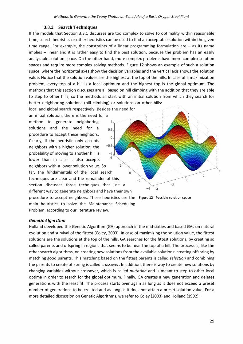
Methods to Generate the Yearly Shutdown-Schedule of a Basic Oxygen Steel Plant
29
3.3.2 Search Techniques
If the models that Section 3.3.1 discusses are too complex to solve to optimality within reasonable
time, search heuristics or other heuristics can be used to find an acceptable solution within the given
time range. For example, the constraints of a linear programming formulation are – as its name
implies – linear and it is rather easy to find the best solution, because the problem has an easily
analyzable solution space. On the other hand, more complex problems have more complex solution
spaces and require more complex solving methods. Figure 12 shows an example of such a solution
space, where the horizontal axes show the decision variables and the vertical axis shows the solution
value. Notice that the solution values are the highest at the top of the hills. In case of a maximization
problem, every top of a hill is a local optimum and the highest top is the global optimum. The
methods that this section discusses are all based on hill climbing with the addition that they are able
to step to other hills, so the methods all start with an initial solution from which they search for
better neighboring solutions (hill climbing) or solutions on other hills:
local and global search respectively. Besides the need for
an initial solution, there is the need for a
method to generate neighboring
solutions and the need for a
procedure to accept these neighbors.
Clearly, if the heuristic only accepts
neighbors with a higher solution, the
probability of moving to another hill is
lower than in case it also accepts
neighbors with a lower solution value. So
far, the fundamentals of the local search
techniques are clear and the remainder of this
section discusses three techniques that use a
different way to generate neighbors and have their own
procedure to accept neighbors. These heuristics are the
main heuristics to solve the Maintenance Scheduling
Problem, according to our literature review.
Genetic Algorithm
Holland developed the Genetic Algorithm (GA) approach in the mid-sixties and based GAs on natural
evolution and survival of the fittest (Coley, 2003). In case of maximizing the solution value, the fittest
solutions are the solutions at the top of the hills. GA searches for the fittest solutions, by creating so
called parents and offspring in regions that seems to be near the top of a hill. The process is, like the
other search algorithms, on creating new solutions from the available solutions: creating offspring by
matching good parents. This matching based on the fittest parents is called selection and combining
the parents to create offspring is called crossover. In addition, there is way to create new solutions by
changing variables without crossover, which is called mutation and is meant to step to other local
optima in order to search for the global optimum. Finally, GA creates a new generation and deletes
generations with the least fit. The process starts over again as long as it does not exceed a preset
number of generations to be created and as long as it does not attain a preset solution value. For a
more detailed discussion on Genetic Algorithms, we refer to Coley (2003) and Holland (1992).
Figure 12 - Possible solution space

Methods to Generate the Yearly Shutdown-Schedule of a Basic Oxygen Steel Plant
30
Baskar et al. (2003) apply GA to the Maintenance Scheduling Problem, but they only use it for small
instances and they adapt the approach to make it suitable to their problem. Wang and Hanschin
(2000) also apply and adapt the GA to suit to their Maintenance Scheduling Problem, such that the
storage space and decoding time decrease. Due to these decreases, the computation time becomes
shorter, which may be of use for our research.
Tabu Search
This explanation on Tabu Search (TS) is based on Hertz et al. (2003) and Glover et al. (1993). TS uses a
memory (the tabu list), not only to compare the values of the current objective and best objective,
but also to compare the values of variables and objectives of earlier steps. Every step in searching for
a new solution starts with evaluating all neighboring solutions (change the variables), followed by
choosing the best of these solutions that is not on the tabu list. Instead of complete solutions, the
tabu list may also contain characteristics of solutions that are not allowed. Several mechanisms can
be chosen to make the algorithm stop, for example if every neighboring solution is on the tabu list or
a certain time window has passed. Of course, there are many approaches to this broad explanation
of tabu search.
The literature does not discuss many approaches to the Maintenance Scheduling Problem that solely
uses TS, because usually researchers combine it with other approaches. Burke and Smith (2000) for
example apply a memetic approach (to start a genetic algorithm with good initial solutions) that
employs TS in order to improve the found schedule. They state that this method is applicable to
large-scale problems, whereas other models, such as the model of Satoh and Nara (1991) are solely
applicable to small-scale problems. On the other hand, El-Amin et al. (2000) apply only TS to solve a
MILP of the Maintenance Scheduling Problem in the power industry. Their conclusion is that the TS
approach is good and promising for further usage based on a comparison with an enumeration
method, but they do not compare it with other search techniques. Gopalakrishnan et al. (2001) also
add a tabu search heuristic to previously performed research and decrease the optimality gap from
2.26% to 0.60%. Again, they do not compare their results with the results of other search heuristics.
Simulated Annealing
We discuss Simulated Annealing (SA) more extensively than TS and GA, because Chapter 4 concludes
that this is the most suitable approach to our problem. Kirkpatrick et al. (1983) developed the SA
method and based it on the Metropolis algorithm (Metropolis et al., 1953). The latter method shows
that natural systems can be used to search for rather good solutions. They take N imaginary particles,
put them in a random structure and calculate the energy of the whole system. Then they rearrange
one particle, again calculate the energy of the system, and compare it with the energy before the
change. If this energy is lower, the algorithm accepts the new structure, otherwise a new change is
proposed based on the previous structure (with the lowest energy).
Now, Kirkpatrick et al. (1983) worked out this idea by comparing it to the annealing of materials, so
melting the material and then slowly let the temperature decrease such that the pattern becomes
more and more fixed. For every decrease in temperature, the pattern changes in order to attain a
steady state and finally – if the temperature is at a preset point – the structure is fixed and changes
are impossible. To apply this idea to find solutions for an optimization problem, Kirkpatrick et al.
(1983) start with a high temperature in which the algorithm moves through the whole solution space
by accepting worse solutions. If the temperature decreases, the search becomes more local (the
solution space is more fixed), meaning that the acceptance of a solution is more and more based on

Methods to Generate the Yearly Shutdown-Schedule of a Basic Oxygen Steel Plant
31
its solution value and less on a random probability, until the temperature is low enough to make the
search algorithm a local search where it only accepts improvements. Kirkpatrick et al. (1983)
conclude that performing SA to a problem requires four aspects:
1) A concise description of a configuration of the system.
2) A random generator of "moves" or rearrangements of the elements in a configuration.
3) A quantitative objective function containing the trade-offs that have to be made.
4) An annealing schedule of the temperatures and length of times for which the system is to be
evolved.
For a much more elaborated overview of SA with explanations of different cooling schedules we refer
to Aarts et al. (1997).
The literature widely describes the use of SA to solve the Maintenance Scheduling Problem, for
example Mohanta et al. (2007) use a combination of a GA and SA to solve the Maintenance
Scheduling Problem. They distinguish between a stochastic and deterministic objective, where
obviously the deterministic function is most comparable to our situation. Satoh and Nara (1991)
research the Maintenance Scheduling Problem for thermal generator maintenance and formulate
the problem as a mixed integer linear programming (MILP) model, which they solve by using SA. They
use penalty functions on some tight restrictions in order to make sure that a feasible solution will be
found, while the deviation from the initial model is the smallest possible. Finally, Saraiva et al. (2011)
formulate the generator Maintenance Scheduling Problem as a mixed-integer problem and use SA to
solve it. They conclude that SA performs very well with a short computation time, but they do not
compare their results with the results attained by enumeration or other search methods.
3.4 Concluding Remarks To conclude, throughout the literature the most applied technique to model the Maintenance
Scheduling Problem is a Mixed Integer Programming technique, whereas the Linear Programming
approach is the least applied technique. Probably because of the usage of non-linear models, most
literature describes a search heuristic to obtain an acceptable solution and the majority of these
researches use Simulated Annealing. Several researches apply Genetic Algorithms and some use
Tabu Search. Combinations of these three local search heuristics are hardly used. Which approach to
apply depends on the specific problem and Chapter 4 continues on this discussion with respect to
Tata Steel’s Maintenance Scheduling Problem. Finally, a search algorithm requires an initial solution,
a neighborhood structure, an acceptance criterion, and a way to measure the quality of the solution.

Methods to Generate the Yearly Shutdown-Schedule of a Basic Oxygen Steel Plant
32
4. Model of the Maintenance Scheduling Problem at Tata Steel This chapter answers the third sub-question of this research: What is the most suitable option to
improve the current method of scheduling shutdowns, taking into account the method’s clarity and
understandability, such that the flow is guaranteed and the restrictions are met? In order to answer
this question, we described several ways to formulate and solve the problem in Chapter 3, which
have to be compared with each other in order to select the most suitable option for scheduling
maintenance at Tata Steel. Section 4.1 covers the analysis and comparison of the different options to
formulate the problem; Section 4.2 formulates the model and compares the formulation with the
formulations in the literature. Section 4.3 selects and describes the local search heuristic to solve the
problem and Section 4.4 contains a conclusion on this chapter.
4.1 Evaluation of the Modeling Techniques This section evaluates the modeling techniques that Section 3.3 discusses and selects the most
suitable option to mathematically model the scheduling problem that Tata Steel faces.
Our problem, as Section 4.2 explains, requires integer variables to set for example the start times of
the jobs and to check whether or not a combination is down. Besides these integer variables, we do
require continuous variables as well to formulate the problem properly, for example to calculate the
overflow of pig iron. Furthermore, the more complex problems that the literature discusses all
require a search technique to obtain good solutions. Our problem is characterized by a high
complexity and, as appears in Section 4.2, linearity cannot be attained. To conclude, we model the
problem as a Mixed Integer Program (MIP), which corresponds to the most used modeling technique
applied in the literature, as Table 2 shows.
4.2 Mathematical Model of the Maintenance Scheduling Problem This section covers the development of the model that can be used to generate the YSS. In order to
model the problem, Section 4.2.1 explains the input and required output, and then Section 4.2.2
stepwise develops the model, based on the requirements.
4.2.1 Model’s Input and Output
This section briefly explains the available input and the required output. Section 4.2.2 develops the
model by explaining the objective and the different constraints step by step.
Input
Currently, Tata Steel generates the YSS based on discussions with the representative sections that
maintain the installations, instead of based on the PO-plans in SAP, which contain the section’s jobs.
Our model uses these PO-plans, because it decreases the subjectivity (i.e., the clarity and
understandability increase) and speeds up the process of searching for required jobs. Moreover, by
using the PO-plans, the jobs instead of the installations are scheduled, which increases the
understandability and the adaptability of the YSS, because it supports the possibility to check when a
specific job is scheduled. In addition, by scheduling the jobs that are stored in SAP instead of the
installations, every job is scheduled, whereas the current approach does not schedule every job.
Hence, by using the jobs as input, the sections do not require additional requests for performing a
job that does not fit in the schedule with installations.

Methods to Generate the Yearly Shutdown-Schedule of a Basic Oxygen Steel Plant
33
Although the PO-plans have entries for all required data to schedule the maintenance properly, the
duration and priority of a job usually lack. Obviously, we need the duration of the jobs to schedule
the maintenance, so Tata Steel has to estimate the non-available durations and we require the
priorities to determine the allowed deviation of the cycle time and assign a standard range of [cycle
time - 10%; cycle time + 10%] to the jobs, unless the priority is specified. Finally, Tata Steel bases the
YSS on the downtimes of the Blast-Furnaces and the Direct Sheet Plant (DSP), so these downtimes
function as input. Figure 13 shows the format of the input to the model.
In order to formulate the problem in a mathematical model, we require the following terms:
Decision variables: Variables that change due to decisions made. In our case, the only
decision variable is the moment to start maintenance on an installation.
Parameters: Constant numbers that do not change during scheduling the shutdowns. An
example of a parameter in our case is the amount of Blast-Furnaces.
Auxiliary variables: Variables that change during the solving of the problem. For example,
whether or not an installation is down at time t is a variable, because this is a value that
changes due to decisions on the decision variable (if it is decided that a job will be performed
at time t, the installation corresponding to that job will be down at time t).
Desired Output
In the current lay-out of the YSS, the horizontal axis shows the installations and the vertical axis
shows the time in weeks. From a site-wide point of view, a mirrored lay-out is preferred: the
installations on the vertical axis and the time on the horizontal axis. Besides that preference from a
site-wide point of view, the only additional requirement of the Basic Oxygen Steel Plant is their
preference to a schedule based on hours. Furthermore, the model should represent the problem of
scheduling jobs, in which four objectives appear, which have a different importance ranking and the
next three paragraphs discuss these.
The primary objective of scheduling the shutdowns is to prevent dumping at Harsco or deregulating
the Blast-Furnaces, which consequently is the primary objective of the method we develop. This
corresponds to the objective of minimizing the ‘Loss of Load Expectation’ (LOLE), which frequently
appears in the literature, see among others Suresh and Kumarappan (2012). The method does not
have to distinguish between dumping at Harsco and deregulating the Blast-Furnaces, because a year
in advance it is not possible to determine which option to select.
The secondary objective is to prevent working in overtime, which is performing maintenance
between 7am and 3pm or during the weekends. The tertiary objective is to prevent deviating from
the cycle time, so if a job has a cycle time of ten weeks, the objective should be to stay as close to
Figure 13 - Format of input requirements
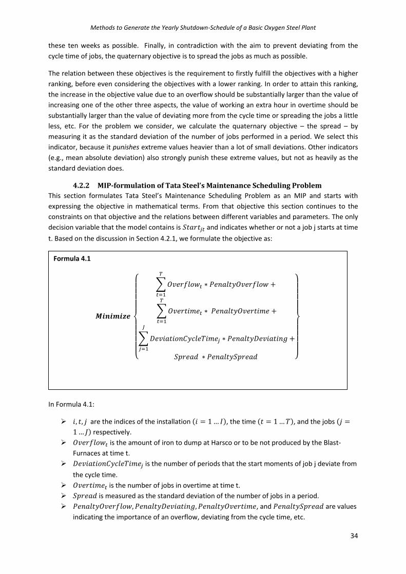
Methods to Generate the Yearly Shutdown-Schedule of a Basic Oxygen Steel Plant
34
these ten weeks as possible. Finally, in contradiction with the aim to prevent deviating from the
cycle time of jobs, the quaternary objective is to spread the jobs as much as possible.
The relation between these objectives is the requirement to firstly fulfill the objectives with a higher
ranking, before even considering the objectives with a lower ranking. In order to attain this ranking,
the increase in the objective value due to an overflow should be substantially larger than the value of
increasing one of the other three aspects, the value of working an extra hour in overtime should be
substantially larger than the value of deviating more from the cycle time or spreading the jobs a little
less, etc. For the problem we consider, we calculate the quaternary objective – the spread – by
measuring it as the standard deviation of the number of jobs performed in a period. We select this
indicator, because it punishes extreme values heavier than a lot of small deviations. Other indicators
(e.g., mean absolute deviation) also strongly punish these extreme values, but not as heavily as the
standard deviation does.
4.2.2 MIP-formulation of Tata Steel’s Maintenance Scheduling Problem
This section formulates Tata Steel’s Maintenance Scheduling Problem as an MIP and starts with
expressing the objective in mathematical terms. From that objective this section continues to the
constraints on that objective and the relations between different variables and parameters. The only
decision variable that the model contains is and indicates whether or not a job j starts at time
t. Based on the discussion in Section 4.2.1, we formulate the objective as:
In Formula 4.1:
are the indices of the installation ( ), the time ( ), and the jobs (
) respectively.
is the amount of iron to dump at Harsco or to be not produced by the Blast-
Furnaces at time t.
is the number of periods that the start moments of job j deviate from
the cycle time.
is the number of jobs in overtime at time t.
is measured as the standard deviation of the number of jobs in a period.
, and are values
indicating the importance of an overflow, deviating from the cycle time, etc.
{
∑
∑
∑
}
Formula 4.1
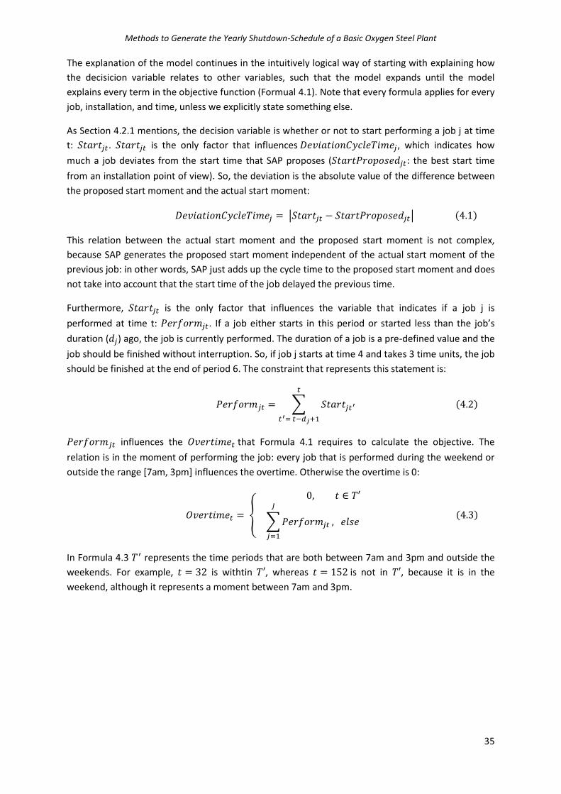
Methods to Generate the Yearly Shutdown-Schedule of a Basic Oxygen Steel Plant
35
The explanation of the model continues in the intuitively logical way of starting with explaining how
the decisicion variable relates to other variables, such that the model expands until the model
explains every term in the objective function (Formual 4.1). Note that every formula applies for every
job, installation, and time, unless we explicitly state something else.
As Section 4.2.1 mentions, the decision variable is whether or not to start performing a job j at time
t: . is the only factor that influences , which indicates how
much a job deviates from the start time that SAP proposes ( the best start time
from an installation point of view). So, the deviation is the absolute value of the difference between
the proposed start moment and the actual start moment:
| | ( )
This relation between the actual start moment and the proposed start moment is not complex,
because SAP generates the proposed start moment independent of the actual start moment of the
previous job: in other words, SAP just adds up the cycle time to the proposed start moment and does
not take into account that the start time of the job delayed the previous time.
Furthermore, is the only factor that influences the variable that indicates if a job j is
performed at time t: . If a job either starts in this period or started less than the job’s
duration ( ) ago, the job is currently performed. The duration of a job is a pre-defined value and the
job should be finished without interruption. So, if job j starts at time 4 and takes 3 time units, the job
should be finished at the end of period 6. The constraint that represents this statement is:
∑ ( )
influences the that Formula 4.1 requires to calculate the objective. The
relation is in the moment of performing the job: every job that is performed during the weekend or
outside the range [7am, 3pm] influences the overtime. Otherwise the overtime is 0:
{
∑
( )
In Formula 4.3 represents the time periods that are both between 7am and 3pm and outside the
weekends. For example, is withtin , whereas is not in , because it is in the
weekend, although it represents a moment between 7am and 3pm.

Methods to Generate the Yearly Shutdown-Schedule of a Basic Oxygen Steel Plant
36
is also the only factor that influences the spread of jobs over the time horizon: .
The spread indicates the equality of the amount of jobs that have to be performed in a period. As
Section 4.2.1 mentions, we measure by means of the standard deviation, which is the square
root of the variance. In our case the formula of the variance depends on the amount of jobs at period
t. The spread equals the square root of the variance and we analyze the entire population:
√
∑(∑
∑∑
)
( )
So far, the model explains three of the four parts that form the objective value. The rest of this
section models the relationship between the height of the overflow at time t ( ) and the
moments to perform a job ( ).
First, an installation i is down at time t ( ) if a job is performed on that installation at time
t. So, is 1, if is 1 for one of the jobs on installation i. In Formula 4.5
represents the set of all jobs j that require installation i, such that means for every job in the
set of jobs on installation i.
{ } ( )
Section 2.4 explains the influence of the down-being of an installation on the cycle time and
concludes that the cycle time through the Basic Oxygen Steel Plant at time t ( )
depends on the down-being of certain combinations of installations. A combination c of installations
is down at time t ( ), if is 1 for every installation in that combination at time
t. If is 1, the cycle time through the Basic Oxygen Steel plant is at least a pre-defined cycle
time that corresponds to that combination ( ). Obviously, only the maximum cycle time applies:
{ } ( )
Based on this cycle time, we know the capacity of the Basic Oxygen Steel Plant at time t:
( )
Besides the capacity of the Basic Oxygen Steel Plant, the model requires the input of pig iron from
the Blast-Furnaces and the input of pig iron from the hot metal cars to calculate the overflow. The
output of the Blast-Furnaces at time t ( ) is made up of two parameters: the
production speed of Blast-Furnace F at time t ( ) and whether or not Blast-Furnace F
is up at time t ( ). Now, the total output of the Blast-Furnaces at time t equals:
∑
( )

Methods to Generate the Yearly Shutdown-Schedule of a Basic Oxygen Steel Plant
37
The input at the Basic Oxygen Steel Plant at time t ( ) depends on the available pig iron
(the height of the buffer in hot metal cars that is left from the previous period ( ) plus
output of the Blast-Furnaces) and the capacity of the Basic Oxygen Steel Plant. Moreover, the input
equals the minimum of these two values, because we assume that the amount in the hot metal cars
decreases as quick as possible, to keep the temperature as high as possible:
{
} ( )
The amount of iron in the hot metal cars ( ) at the end of time t depends on the amount
of iron in the hot metal cars in the previous period and the change in the of amount pig iron in the
current period ( ):
( )
The change in the buffer depends on the difference between the output of the Blast-Furnaces and
the input at the Basic Oxygen Steel Plant, but may never be more than the difference between the
capacity of the hot metal cars ( ) and the buffer in the previous period
( ):
{
} ( )
Clearly, the output of the Blast-Furnaces that can neither be stored in hot metal cars, nor be
processed by the Basic Oxygen Steel Plant, is the overflow of pig iron ( ):
( )
Finally:
{ }
{ }
{ }
{ }
4.2.3 Differences with Literature
The model that we obtain from Section 4.2.2 is neither linear nor using solely continuous variables,
so we typify the model as a Mixed Integer Programming (MIP) formulation of the Maintenance
Scheduling Problem, which is the main technique applied in the literature, as Table 2 shows.
The main difference with the models in the literature is in the complexity of the objective function.
Although Kralj and Petrović (1988) discuss that the Maintenance Scheduling Problem has multiple
objectives, they conclude from their literature review that most authors optimize the problem based
on only one objective. Most authors use the costs as the only objective (e.g., Saraiva (2011)),
whereas we add the availability of personnel, the optimality of the previously defined cycle times,

Methods to Generate the Yearly Shutdown-Schedule of a Basic Oxygen Steel Plant
38
and the manageability of maintenance to the objective. On the other hand, some authors (e.g.,
Chattopadhyay et al. (1995) and Berrichi (2009)) combine the scheduling of maintenance with the
production schedule, which increases the complexity of the restrictions and the solving method.
Nevertheless, such an approach compares to the inclusion of the cycle times in our MIP formulation.
These cycle times represent the production, which is a continuous process, such that minimizing the
total cycle time equals to maximizing the output of steel.
The main similarities with the literature are our usage of both integer and continuous variables and
the non-linearity of the model. According to Kralj and Petrović (1988) and based on our own
literature research in Chapter 3, most problems require integer variables to set the start moment of
a job and most models are non-linear.
4.3 Implementing the Local Search Technique We are not able to solve the problem by exact methods, because we use an MIP formulation, such
that we require a heuristic approach to solve the Maintenance Scheduling Problem. This section
starts with an analysis of the local search heuristics that Chapter 3 discusses and analyzes the
suitability of the several heuristics to Tata Steel’s Maintenance Scheduling Problem in Section 4.3.1.
Section 4.3.2 continues by explaining how we implement the heuristic that we select and Section
4.3.3 explains how we deal with the ranking in the objectives. Finally, Section 4.3.4 explains some
additional approaches that we apply to solve the Maintenance Scheduling Problem.
4.3.1 Analysis of Search Techniques
We only discuss search heuristics in this section, because the Maintenance Scheduling Problem does
not compare to problems for which useful and good heuristics exist, as Section 3.2 explains.
Probably, that is why previous research does not discuss approaches that use non-search heuristics.
Section 3.2.3 discusses three search algorithms that show their use to the Maintenance Scheduling
Problem in the literature: Genetic Algorithms (GA), Tabu Search (TS), and Simulated Annealing (SA).
In order to select the most suitable search algorithm for our problem, this paragraph discusses the
advantages and disadvantages of these algorithms, but first and above all we state that the selected
option heavily depends on the model’s specificities, such that this approach is not per definition the
most suitable approach for comparable problems. Burke et al. (1997) compare SA, TS, GA, and a
combination of the first two methods for a simplified and broadly defined Maintenance Scheduling
Problem and conclude that GA is the worst performing algorithm for larger feasible solution spaces,
but it performs better than SA for smaller solution spaces. Our solution space is very large, especially
because of the high amount of jobs that have to be scheduled.
Besides the large number of jobs, Tata Steel prefers to use a large amount of periods, which makes
the problem’s solution space even larger. The amount of neighboring solutions negatively influences
the suitability of Tabu Search, because TS requires that every neighbor is analyzed and selects the
best (non-tabu) option as the new solution. Clearly, the amount of neighbors depends on the
neighborhood structure, but TS analyzes every neighbor before moving to another solution. This
requires a lot of computation time to compare the different solutions before moving through the
solution space. Still, Burke et al. (1997) conclude that TS outperforms the other approaches, whereas
Ruiz et al. (2007) conclude the contradictory idea about their flow-shop problem. So, again the most
suitable option heavily depends on the analyzed problem.

Methods to Generate the Yearly Shutdown-Schedule of a Basic Oxygen Steel Plant
39
The GAs have a high computation time, due to the complicated decoding computations and the
heavy fitness evaluations in each generation, according to Wang and Hanschin (1999). So, both GAs
and TS spend a lot of time on evaluating the solution, while this computation time should be used to
generate improvements in the solutions. Our problem requires that the algorithm quickly moves
through the solution space because of the high amount of solutions with the same objective value,
which indicates that Tabu Search does not suit the problem.
On the other hand, Simulated Annealing quickly analyzes a lot of different solutions and moves
through the solution space with a speed corresponding to the time/temperature the method runs.
Another positive point of SA is the clear convergence towards a local optimum after – as we expect –
having searched most hills. Additionally, SA does not require a good initial solution, because it finds
high quality solutions which do not strongly depend on this initial solution (Aarts & Korst, 1989).
Based on the discussion above and the model we develop in Section 4.2, we conclude that Simulated
Annealing suits best to the Maintenance Scheduling Problem that Tata Steel faces.
In our view the most important disadvantages are the amount of feasible solutions and the fact that
the solution space contains many local optima. The local optima are not necessarily global optima,
because SA creates clusters which are not necessarily scheduled during a plant-shutdown. Section
4.3.3 explains difficulties with local optima and explains how our method deals with this difficulty.
Another important disadvantage is the required fine-tuning of the parameters in SA (initial
temperature, decrease factor, stop criterion), which has to be repeated when the problem changes.
Section 4.3.2 explains how to determine these parameters.
To conclude, we solve the Maintenance Scheduling Problem, which we formulate in Section 4.2.2 as
Mixed Integer Program, by using Simulated Annealing. Section 4.3.2 explains how we apply SA to the
scheduling problem of Tata Steel.
4.3.2 Implementing Simulated Annealing
As Section 4.3.1 shows, we require Simulated Annealing to solve the Maintenance Scheduling
Problem of Tata Steel. This section explains the implementation of Simulated Annealing and the
determination of the variables to apply SA. Section 3.3.2 mentions four requirements to apply SA,
namely:
1 A concise description of a configuration of the system.
2 A random generator of "moves" or rearrangements of the elements in a configuration.
3 A quantitative objective function containing the trade-offs that have to be made.
4 An annealing schedule of the temperatures and length of times for which the system is to be
evolved.
Section 4.2 covers the first requirement by expressing the problem in an MIP-formulation, which
describes the problem and the embedded relations between the variables. The third requirement
corresponds to the objective of the model (Formula 4.1) that Section 4.2 explains, together with the
representativeness of this objective and the corresponding dilemma in it. Both requirement 2 and 4
comprise the actual local search procedure of SA. The remainder of this section discusses these
requirements.

Methods to Generate the Yearly Shutdown-Schedule of a Basic Oxygen Steel Plant
40
Neighborhood Structure
The second requirement encompasses the determination of the neighborhood structure, as Chapter
3 explains. In order to adapt a schedule, SA requires an initial schedule and, as Section 3.3.2
mentions, an advantage of SA is the robustness and effectiveness, such that it does not necessarily
require a good initial solution. Hence, we set the start moment of a job to 7am on the date it should
be performed according to its PO-plan, because this reduces the overtime value and deviation from
the cycle time value in the objective function.
Based on the previous solution, it is allowed for SA to reschedule the jobs within certain bounds,
which we based on the priority of a job as indicated in SAP. Usually the priority is equal to its initial
value of 1 (highest priority: the job has to be performed close to the proposed start moment), which
means that the sections did not change the priority of the jobs. We assigned both a lower bound and
an upper bound of 10% of its cycle time to these jobs with priority 1: the bounds of a job equal to the
proposed start moment plus and minus 10% of the job’s cycle time. This results in 2,460,853 possible
start moments for 2287 jobs (on average approximately 1076 moments to start a job). With each
step, SA randomly selects a job out of the 2287 jobs and assigns a new start moment to that job,
which it randomly selects out of the allowed start moments of the job.
The primary objective is to attain a minimum overflow, which probably means that several jobs
should be performed when the buffer does not contain any steel. Of course, we recognize these jobs
on some characteristics (high duration, an installation that influences the cycle time). Hence, we
admit that every year’s schedule contains jobs with certain characteristics on which smarter moves
can be based, but these characteristics are that specific and different for every job and depend on
other installations that are down (combinations influence the cycle time). In order to create an
understandable approach that requires the least adaptions as possible when a new YSS has to be
created, we apply the completely random generator of moves.
Annealing Schedule
The annealing schedule aims to start searching globally for new schedules and to finish searching
locally for new schedules. In order to comply to this requirement, the procedure does not only
accept a neighbor if the objective value of the neighbor is better than the current configuration’s
objective value (the hill-climbing idea, Figure 12), but also accepts neighbors with a worse objective
value with a certain probability. This probability equals to (
),
where the temperature needs to be specified by a cooling scheme. For SA to search globally when
the procedure starts, the algorithm should initially accept almost every solution, such that the
acceptance ratio (hence the probability) needs to be very close to 1. When time passes, the
procedure should search more locally, so the search space should become smaller and the
acceptance ratio has to approach 0 at the end of the algorithm. In order to obtain this evolvement of
the acceptance ratio, initially the temperature should be very high compared to the difference in the
objective value and the temperature should be relatively low at the end of the procedure.
The differences between the objectives of two neighboring schedules depend both on the value that
we assign to the penalty of the corresponding objective and on the increase of the objective value.
The penalties indicate when Tata Steel is indifferent between a decrease of one objective at the cost
of an increase of another objective. For example, if the penalties for the overflow, overtime,
deviating from the cycle time, and spread are 100, 10, 1, and 0.1 respectively, Tata Steel is indifferent
between a decrease in the overflow of 1 ton or working 10 hours less in overtime. However, we are

Methods to Generate the Yearly Shutdown-Schedule of a Basic Oxygen Steel Plant
41
not able to select the real points of indifference, because it requires too much time and it is not
needed for the development of the method (Tata Steel can add the correct penalties if these are
available). As Section 4.2.1 explains, we assume that the objectives are strictly ranked, which means
that a lower ranked objective never decreases at the cost of a higher ranked objective. We solely set
the penalties based on that requirement and Appendix C concludes that the penalties for the
overflow, overtime, deviation from the cycle time, and spreading of jobs equal to 1, 1, 0.001, and
0.001 respectively. We admit that these penalties are subjective and do not reflect the actual
importance ranking between the different parts of the objective and we admit that 1 ton overflow of
steel does not correspond to an hour more in overtime, but the approach of SA holds that an
increase in overflow always corresponds to an increase of at least 65 tonnes and because SA only
considers one job per move, SA never accepts a rescheduling move in which the overtime decreases
and the overflow increases. Again, Tata Steel should re-define these penalties for an optimal use of
the method. Section 4.3.3 continues on the usage of the penalties.
4.3.3 Dealing with the Ranked Objectives
For our specific problem with four strictly ranked objectives, SA needs an adaption, because a
standard SA procedure does not correctly optimize the problem. First, this section discusses an
example of incorrect optimization and this section finishes with a better approach.
Figure 14 shows a possible YSS of a situation in which the plant consists of only one Blast-Furnace
and two casting installations. Some jobs require only one casting installation and other jobs require
both casting installations. In Figure 14, the crosses indicate that an installation is down during the
corresponding period. During the shutdown of the Blast-Furnace, there is no supply of pig iron and
no overflow, whereas the overflow during the shutdown of a casting installation equals to 5 tonnes
and if both casting installations are down, the overflow equals to 2 x 5 tonnes. Furthermore, in Figure
14’s YSS every job is performed on its proposed moment, the overtime is 6 periods (only the jobs
during period 6 and 16 affect the overtime), and the spread is 1.58. So, the total objective equals to
10 + 6 + 0/1000 + 1.58/1000 = 16.00158.
Intuitively, maintaining both casting installations should be done during a plant-shutdown, because it
heavily influences the cycle time (from 18 minutes to 90 minutes). However, an SA procedure that
analyzes all objectives at once does not accept any change of a casting installation in this schedule:
for example, if it moves a job from period 12 to start in period 6, the overflow of ten remains the
same (still both casting installations are down), the overtime of 6 remains 6, the deviation of the
cycle time increases to 7 – which should be divided by 1000 – and the spread increases to 1.87 –
which should be divided by 1000. So, the new objective value becomes 10 + 6 + 7/1000 + 1.87/1000 =
16.88. SA does not accept any move in Figure 14, if it approaches the lower bound on the
temperature (i.e., the solution is a local optimum). Hence, optimizing all objectives at once leads to a
bad local optimum.
In order to prevent this problem, we first run the SA procedure with just minimizing the overflow as
objective, then if this procedure finishes, we take the best schedule so far and recalculate the
objective with the addition of the secondary objective. Based on the new objective and the same
schedule, we start SA again and repeat this until the SA procedure contains every objective. By using
this four-run SA approach, the configuration in Figure 14 is not a local optimum, because every job
may be moved to the upper half of Figure 14 during the first run. These moves decrease the
objective, such that the first run only ends if all jobs are moved to the upper half.

Methods to Generate the Yearly Shutdown-Schedule of a Basic Oxygen Steel Plant
42
YSS Installation
Period BF 1 Casting
Installation 21 Casting
Installation 22 Casting Installation
21 + 22
1 X
2 X
3 X
4 X
5 X
6 X X X X
7 X X X X
8 X X X X
9 X X X X
10 X X X X
11
12 X X X
13 X X X
14 X X X
15 X X X
16 X X X
17
18
19
20 Figure 14 - A part of a possible YSS
The four-run SA requires four start temperatures and four stop criterions – both for every run. Table
3 shows these temperatures, which we calculated based on the explanation in Appendix C. We used
the following computations to calculate the temperatures:
In order to make sure that SA accepts every neighboring schedule when the procedure starts,
(
) should approach one and . So, the current objective
minus the neighboring objective should be substantially smaller than the temperature. The maximum
difference between the objectives in the first run equals to 6160, as Appendix C shows. In order to
attain a starting probability of 0.98, the temperature should equal:
(
)
The minimum difference in the first run equals to 68 and the probability of accepting a worse
solution should be equal to 0.01, such that the final temperature should be equal to:
(
)
We understand that these temperatures lead acceptance ratios of more than 98% and less than 1%,
because most neighboring objectives do not differ with a value of 6185 and 68 respectively. Still, we
use this approach to make the determination of these parameters easier to repeat for Tata Steel. For
determining better temperatures, we should use the actual acceptance ratios after a run.

Methods to Generate the Yearly Shutdown-Schedule of a Basic Oxygen Steel Plant
43
Table 3 - Start and final temperatures of the four different runs of SA
In order to use the values in Table 3, every chain should finish in a local optimum, such that the next
run solely focusses on the last added objective. By using this adapted SA version, Figure 14’s bad
local optimum does not appear anymore.
Finally, we require the right balance between the length of the markov chain and the speed of
decreasing the temperature. First, to make the procedure not too complex and keep the procedure
understandable for Tata Steel, we set an equal decreasing factor and chain length to each of the four
runs. Furthermore, we prefer SA to put most of its effort in local search, so we set the decreasing
factor very high compared to the markov chain length. Another possibility or addition is to make the
markov chains increase with a decrease in the temperature, but this unnecessarily increases the
complexity of the method. We set the decreasing factor to 0.99975, such that SA analyzes
( ⁄ )
( ⁄ )
(
⁄ )
(
⁄ )
In order to analyze the results in Excel, we set the decreasing factor to 0.99975, because Excel 2003
can deal with at most 65,000 rows. This means that the maximum chain length – run 3: 60,614 –
influences the decreasing factor and based on the number of chains and the computation time, we
set the markov chain length equal to 100. By selecting a higher value to the decreasing factor and a
lower value to the chain length, the time that SA spends in searching locally increases. So, setting the
decreasing factor equal to 0.9999975 and the chain length equal to 1 results in the same amount of
solutions, but also makes sure that SA spends more time searching locally. However, these
differences do not significantly influence the result.
4.3.4 Additional Approaches to the Maintenance Scheduling Problem
This section discusses alternatives for searching for a local optimum. In order to compare the
different methods, we select the parameters that characterize the approaches such that the
runtimes of the different approaches are equal.
For the four-run SA we set the four start and four stop temperatures equal to the temperatures that
Section 4.3.3 discusses, but we set the decreasing factor to 0.999, because this improves the usability
and comparability of the results. In order to attain an equal computation time for every heuristic, the
four-run SA uses a markov chain length of 3.
Besides the four-run SA approach, we also apply Simulated Annealing with only one run to obtain a
YSS. This conventional SA approach optimizes all four parts of the objective together and we expect
that this approach finds a local optimum in relatively short computation time, as Section 4.3.3
explains. Hence, we expect that this approach outperforms the four-run SA method in the
experiment, but it should also show that the four-run SA did not find a local optimum when the
Objective/Run: Overflow/1 Overtime/2 Deviation CT/3 Spread/4
Maximum Difference 6160 8 1680/1000 = 1.68 0.15/1000 = 0.00015
Minimum Difference 68 1 1/1000 = 0.0001 0.01/1000 = 0.00001
Start Temperature 304910 396 84 0,007
Final Temperature 14 0.22 2.2*10-5 2.2*10-6

Methods to Generate the Yearly Shutdown-Schedule of a Basic Oxygen Steel Plant
44
experiment ends. Finally, we set the start temperature equal to the start temperature of the first run
of the four-run SA method and the lower bound on the temperature equal to the lower bound on the
temperature in the final run of the four-run SA method, because the possible increase in the
maximum difference in the objective value between two neighboring solution is negligible. We set
the decreasing factor equal to 0.999 – to compare it with the four-run SA – and the chain length
equal to 8, such that the runtime equals the runtime of the other alternatives.
Next to the SA approaches, we evaluate an iterative improvement method – in the remainder of this
chapter called IIM – to obtain a solution to the problem. This method takes into account the
overtime by rescheduling the start moment of a job such that it starts on another day at 7am. This
heuristic starts by analyzing the solution if the first job is scheduled 24 hours later and continues with
this job until it analyzed every start moment of this job as long as the job starts at 7am and within the
allowed bounds. After analyzing the first job, the heuristic continues with the next job, until it
analyzed every job. Finally, this procedure repeats for a preset number of iterations. Our decision to
start at 7am and not to analyze every possible start moment is especially based on the decrease in
the solution space by 96%. To comply with the runtime restriction, this IIM iterates 15 times over all
jobs. In addition, we apply the same IIM heuristic that changes the start time with 8 hours instead of
24 hours and which iterates 5 times instead of 15 times over all jobs.
Finally, we implement a combination of SA with one run and IIM. This combined approach starts with
SA and finishes with IIM, based on the solution obtained with SA. We dedicate the first 50% of the
runtime to the SA approach and the last 50% of the runtime to the IIM part, which means that it
starts with the same cooling scheme as the approaches that solely use SA, but the markov chain
length decreases to 3 and it ends with an IIM with 7 iterations over all jobs, with the same approach
as the heuristic that solely uses iterative improvement with steps of 24 hours.
We admit that several other approaches seem to be worth analyzing, such as another neighborhood
structure, another search heuristic, or other combinations of and parameters in the heuristics that
the previous paragraphs explain. However, the options we select clarify the potential of the type of
heuristics.
4.4 Concluding Remarks To conclude, we modeled Tata Steel’s Maintenance Scheduling Problem in Mixed-Integer
Programming formulation, which we solve in four steps of Simulated Annealing (SA). The SA selects a
neighboring solution by randomly selecting a job and subsequently randomly selecting a new
moment to start that job. The four steps comprise a SA procedure that solely optimizes the overflow
objective, until it reaches a local optimum. Based on that schedule, the objective enlarges with the
overtime and a new SA procedure starts. These steps continue until the objective contains the
overflow, the overtime, the deviation from the cycle time, and the spread. Besides this four-run SA
approach, Chapter 5 contains an analysis and comparison of four relatively simple alternative
approaches to solve the Maintenance Scheduling Problem.

Methods to Generate the Yearly Shutdown-Schedule of a Basic Oxygen Steel Plant
45
5. Analysis and Discussion of the Results This chapter answers the fourth research question: What are the results of applying the selected
method? First, Section 5.1 describes the initial solution we used. Section 5.2 analyzes the
performance of the SA heuristic that we applied and the performance of alternative heuristics.
Section 5.3 reflects on the rules of thumb, contains an analysis of the results, discusses the appearing
shortcomings of the approach, and sets forth possible improvements to prevent the shortcomings.
Furthermore, Section 5.3 compares the schedule we obtained with the YSS as Tata Steel generated it.
Section 5.4 reflects on the computation time and Section 5.5 briefly summarizes the analysis.
5.1 Initial Solution The initial solution holds that every job is scheduled on the start date in its PO-plan, so the deviation
from the cycle time equals zero in the initial objective value. Furthermore, the jobs start at 7am,
which means that the overtime is rather low in the initial solution, but jobs in the weekends have an
impact on the overtime objective. On the other hand, jobs and – especially – the installations are not
clustered in the initial solution, so we expect an increase in both the overtime and the deviation from
the cycle time and a decrease in both the overflow and the spread, due to the clustering of jobs. The
initial solution has an objective value of 653,066 and is made up of the values in Table 4.
Table 4 - Objective values of the initial solutions
Initial solution
Objective 653,066.4
Overflow 651,066.4
Overtime 2,000
Deviation from CT 0 (/1000)
Spread 5.03 (/1000)
5.2 Performance of Simulated Annealing This section discusses the performance of the four-run Simulated Annealing heuristic that we apply
to the Maintenance Scheduling Problem as well as the performance of the other heuristics (IIM, SA,
combination). First, Section 5.2.1 discusses the performance of the four-run SA heuristic, then
Section 5.2.2 shortly discusses and compares the other four heuristics with each other and with the
four-run SA approach.
5.2.1 Simulated Annealing
As Chapter 4 discusses and Table 3 shows, SA analyzed the solution space in four runs. We expect
that after a run, which is after adding a part of the objective, the higher ranked objectives can never
increase due to the decrease of the new objective. On the other hand, the overall objective
increases, because a new part is added to the objective value. Figure 15 shows the simplified
expected flow of the fictitious objective value: after the first run SA reaches a local optimum and
adds the second objective, such that the objective value increases. Again, SA reaches a local
optimum, which has a higher corresponding objective value than the local optimum after the first
run, because this value contains objective two. This process continues until the objective contains all
four parts and ends up in a local optimum. Furthermore, higher ranked objectives are not able to in-
or decrease when the overall objective includes a lower ranked objective, unless the run did not end
in a local optimum.

Methods to Generate the Yearly Shutdown-Schedule of a Basic Oxygen Steel Plant
46
Figure 15 - Expected flow of the objective value
Table 5 shows the actual values of the objectives after the four runs finished, and specifies the values
that influence the overall objective. In Table 5, only the black colored values influence the objective
value, because the values in red italics are left out of the objective in the corresponding run. Table 5
shows that the decrease in the objective value is mainly due to the decrease in the overflow at the
expense of working a little more in overtime and deviating much more from the cycle time. The small
overtime increase of only 8% indicates that jobs are moved out of the weekend and that only a few
jobs are scheduled during evenings or nights. As the previous paragraph mentions, a part of the
objective cannot change if the overall objective contains a lower ranked objective. However, Table 5
clearly shows a decrease in the overflow, overtime, and deviation from the cycle time in every run in
which it is optimized. This means that none of the runs ended in a local optimum, which either
means that the acceptance ratio is significantly larger than zero, or that the SA method still finds
better solutions. Figure 16 to Figure 19 show the acceptance ratios of the four runs and show that
each run ends with an acceptance ratio of approximately 0%, so the reason for not reaching a local
optimum after a run should be the fact that still better direct neighbors exist. Figure 20 to 23 show
the flow of the objective value in each run and confirms the previous statement. This section
continues with a discussion on the acceptance ratio and the decrease of the objective value.
Table 5 - The flow of the objective values.
Initial 1st run 2nd run 3rd run 4th run Decrease
Objective 653,066.4 110,689 86,648 81,152 74,291 -89%
Overflow 651,066.4 110,689 84,153 78,843 72,067 -89%
Overtime 2,000 11,307 2,495 2,227 2,155 +8 %
Deviation (/1000) 0 603,015 619,900 81,947 69,662 - %
Spread (/1000) 5.03 2.757 3.099 3.995 4.149 -18%

Methods to Generate the Yearly Shutdown-Schedule of a Basic Oxygen Steel Plant
47
Figure 16 - Acceptance ratio of Run 1 of Simulated Annealing
Figure 17 - Acceptance ratio of Run 2 of Simulated Annealing

Methods to Generate the Yearly Shutdown-Schedule of a Basic Oxygen Steel Plant
48
Figure 18 - Acceptance ratio of Run 3 of Simulated Annealing
Figure 19 - Acceptance ratio of Run 4 of Simulated Annealing

Methods to Generate the Yearly Shutdown-Schedule of a Basic Oxygen Steel Plant
49
Acceptance Ratio
As Chapter 4 discusses, the acceptance ratio should start close to 100% and end at almost 0%. This
means that SA accepts almost all deteriorations of the objective value when SA starts and that SA
does not accept any significant deterioration of the objective value at the end of the procedure.
Figure 16 to Figure 19 show the ratio of worse solutions that SA accepted. As the previous paragraph
mentions, all four acceptance ratios end at 0%, which means that SA only accepts improvements and
we do not discuss this any further, because it confirms Chapter 4’s discussion.
On the other hand, the initial acceptance ratios of run two, three, and four do not confirm the
explanation in Chapter 4. The reasoning is rather straightforward: The acceptance ratio of run two
(and run three) starts between 20% and 40%, which means that SA accepts approximately 30% of the
deteriorations in the first stage of the procedure. Hence, 70% does not fit to the evolvement of the
acceptance probabilities calculated by (
), which means that 70%
of all deteriorations is too high with respect to the temperature to be accepted by SA. So, we either
determined the initial temperature in the wrong way, or the differences in the objective value are
higher than we expected. Besides the influence of not reaching a local optimum after the first run,
the main reason for the low initial acceptance ratio in the second run is the fact that SA rejects most
neighbors because it increases the first objective (i.e., the overflow). So, approximately 60% of the
neighbors make the overflow to increase, such that SA does not accept these neighbors. To conclude,
the strange starting acceptance ratios in run two and run three are as they should be and the ending
acceptance ratios make it possible for SA to reach a local optimum.
Figure 20 - Objective value during the first run

Methods to Generate the Yearly Shutdown-Schedule of a Basic Oxygen Steel Plant
50
Figure 21 - Objective value during the second run
Figure 22 - Objective value during the third run
Figure 23 - Objective value during the fourth run

Methods to Generate the Yearly Shutdown-Schedule of a Basic Oxygen Steel Plant
51
Objective Values
As Figure 15 shows, we expected to obtain four pictures such as Figure 20 shows. However, with
each subsequent run the similarity disappears until Figure 23’s evolvement of the objective value
does not show any relevant similarity anymore. This section discusses the differences between Figure
15 and Figure 20, 21, 22 and 23.
First, Figure 15 shows that – optimally – the objective value after a run cannot be lower than the
objective value after the previous run. Table 5 shows that the objective value decreases after every
run and we conclude based on this observation that SA does not reach a local optimum during any of
the runs. Another conclusion that we draw based on Table 5 is that SA clearly minimizes a new
objective after its addition to the overall objective, as the red italics and the first black values in Table
5 indicate. The next paragraphs compare the different runs with the corresponding parts in Figure
15.
Figure 15 indicates that a new run should start with a small increase in the objective value, followed
by a drop in the objective value until it reaches a local optimum in which the objective value does not
change anymore. The evolvement of the objective value in the first run seems to comply to this
statement, but if we zoom-in on the last part of Figure 20, we obtain a surprising evolvement of the
objective value as Figure 24 shows. Chapter 4 explains that the minimum difference between two
neighboring solutions in the first run equals to 64, but Figure 24 clearly shows smaller increases.
These increases should be due to varying occupations of hot metal cars and this should be included
in the future, such that the lower bound on the temperature equals 0.22 (based on a minimum
difference of the objective value of one). Due to this shortcoming in the objective, it is possible for SA
to outweigh an increase in the overflow by a decrease in the overtime during the second run.
Due to the fact that the first run does not end in a local optimum, Figure 21 does not show the
correct evolvement of the objective value, because the deviaton in the overflow still influences the
objective value. First, the increase in the left-hand side of Figure 21 corresponds to our expectations,
which Figure 15 shows. However, the objective value keeps decreasing in the tail of the second run
and never reaches a local optimum and the objective value drops lower than the final objective value
or the first run.
Figure 24 - Final part the evolvement of the objective value during Run 1

Methods to Generate the Yearly Shutdown-Schedule of a Basic Oxygen Steel Plant
52
The third run still shows a small increase in the objective value in its first stage, but run four’s Figure
23 does not show this increase anymore. The dissimilarity between the figures and Figure 15 is
mainly because SA did not reach a local optimum in the first run, such that it is not able to reach a
local optimum in the subsequent runs.
Another issue with respect to the objective value is – although it does not appear in the figures – the
temperature overlap of the different runs. Run three starts with a temperature in which the
acceptance ratio in the previous run was between 40% and 20%. This means that in these runs, the
objective of the previous run is not fixed. Hence, we propose to redefine the start tempertures,
which means that we propose to redefine the penalties. In order to prevent any overlap in the
temperatures and to include the new minimum difference of the overflow we propose using the
penalties to influence the maximum and mininum differences between the objective values of
neighboring solutions. Table 6 shows the resulting penalties and bounds on the temperatures. We
obtained these by using the formulas in Chapter 4. As Chapter 4 mentions, these penalties do not
have to reflect the importance with respect to another objective, but have to influence the
temperatures.
An issue that seems to appear in the figures and Table 5, is the fact that small changes in the
spreading of the jobs appear. Although we did expect small changes in the value for spreading, if the
third run would have reached a local optimum the differences in the spreading would be even
smaller. This is simply because a change in the spreading of jobs always affects the devation in the
cycle time or the amount of overtime. The only option in which it does not influence the overtime,
neither the devation of the cycle time is to reschedule a job exactly the same amount of hours to the
other side of its bound: job j is scheduled at time 40 (not in overtime) and the proposed start
moment is 50, which is a local optimum after the third run. Now, the only option to reschedule job j,
while not changing the deviation of the cycle time and while changing the spread is to reschedule job
j to time 60 (not in overtime). Hence, SA hardly influences the spreading of jobs.
Finally, the difference between the overtime and the deviation of the cycle time in the different runs
may seem odd. These differences are due to the huge increase in the deviation of the cycle time in
the first run at the expense of a decrease in the overflow. During the fourth and espeically during the
third run, the deviaton of the cycle time decreases with a larger value than the decrease in the
overtime. However, this higher decrease is the sum of a lot of small decreases (i.e., a lot of smaller
decreases for the deviation of the cycle time).
5.2.2 Other Approaches
This section analyzes the alternatives for searching for a local optimum, which Chapter 4 explains.
Recall that the alternative heuristics are two Iterative Improvement Methods (IIMs), an SA method,
and a combination of these two methods. These heuristics optimize the four objectives in parallel
instead of subsequently (as the four-run SA does) and we used a short runtime.
Table 6 - Improved temperatures
Run / Objective Penalty Start Temperature Lower Bound on Temperature
1 / overflow 1 304,910 0.20
2 / overtime 5 x 10⁻⁴ 0.20 1.08 x 10⁻⁴
3 / deviation from CT 1 x 10⁻⁹ 8.3 x 10⁻⁵ 2.1 x 10⁻¹⁰
4 / spreading of jobs 2 x 10-11 1.5 x 10⁻¹⁰ 4.3 x 10⁻¹⁴
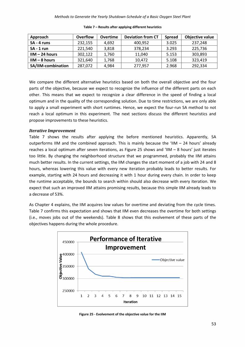
Methods to Generate the Yearly Shutdown-Schedule of a Basic Oxygen Steel Plant
53
Table 7 – Results after applying different heuristics
Approach Overflow Overtime Deviation from CT Spread Objective value
SA - 4 runs 232,155 4,692 400,952 3.025 237,248
SA - 1 run 221,540 3,818 378,234 3.293 225,736
IIM – 24 hours 302,122 1,760 11,040 5.153 303,893
IIM – 8 hours 321,640 1,768 10,472 5.108 323,419
SA/IIM-combination 287,072 4,984 277,957 2.968 292,334
We compare the different alternative heuristics based on both the overall objective and the four
parts of the objective, because we expect to recognize the influence of the different parts on each
other. This means that we expect to recognize a clear difference in the speed of finding a local
optimum and in the quality of the corresponding solution. Due to time restrictions, we are only able
to apply a small experiment with short runtimes. Hence, we expect the four-run SA method to not
reach a local optimum in this experiment. The next sections discuss the different heuristics and
propose improvements to these heuristics.
Iterative Improvement
Table 7 shows the results after applying the before mentioned heuristics. Apparently, SA
outperforms IIM and the combined approach. This is mainly because the ‘IIM – 24 hours’ already
reaches a local optimum after seven iterations, as Figure 25 shows and ‘IIM – 8 hours’ just iterates
too little. By changing the neighborhood structure that we programmed, probably the IIM attains
much better results. In the current settings, the IIM changes the start moment of a job with 24 and 8
hours, whereas lowering this value with every new iteration probably leads to better results. For
example, starting with 24 hours and decreasing it with 1 hour during every chain. In order to keep
the runtime acceptable, the bounds to search within should also decrease with every iteration. We
expect that such an improved IIM attains promising results, because this simple IIM already leads to
a decrease of 53%.
As Chapter 4 explains, the IIM acquires low values for overtime and deviating from the cycle times.
Table 7 confirms this expectation and shows that IIM even decreases the overtime for both settings
(i.e., moves jobs out of the weekends). Table 8 shows that this evolvement of these parts of the
objectives happens during the whole procedure.
Figure 25 - Evolvement of the objective value for the IIM

Methods to Generate the Yearly Shutdown-Schedule of a Basic Oxygen Steel Plant
54
Table 8 - Intermediate results of Iterative Improvement. After iteration 5, the values did not change anymore
Iteration 1 2 3 4 5
Objective 407,744 339,583 317,666 310,081 309,582
Overflow 405,692 337,700 315,841 308,287 307,810
Overtime 2,024 1,857 1,808 1,782 1,760
Devation 28,224 22,800 17,136 12,000 11,616
Spread 5.061 5.100 5.123 5.141 5.139
Simulated Annealing - Iterative Improvement Combination
The combination of SA and IIM shows the same evolvement of the objective value as the approach
that only uses IIM, as Figure 26 shows. Note that both IIM and SA used half of the computation time.
The SA part ends with an objective value of 330,158, which the IIM heuristic approached after two
iterations (at 4/15th of the runtime of SA). So, we propose to adapt this method in the same way as
we propose to adapt the IIM: reducing the amount of periods with which the solution changes in the
IIM part, because the IIM part does influence the objective value by only 13% of the total decrease.
Simulated Annealing – 1 run
Figure 27 shows the objective values and acceptance ratios of the SA heuristic that minimizes the
objective values at once, so without distinguishing between the different objectives by means of
different runs. Figure 27 shows that this SA procedure approaches a local optimum and shows a
decreasing acceptance ratio. Moreover, in this experiment it performs better than any of the other
four heuristics, which is conform our expectations which Chapter 4 discusses. Chapter 4 explains that
we expect this SA approach to find a local optimum quicker, but also explains that we expect that his
local optimum has a lower quality than the local optimum that a four-run SA obtains. Still, this one-
run SA approach performs better on each part of the objective, besides the spread. We think that
this is due to the low runtime during the first run of the four-run SA procedure, but conclude that
Tata Steel could use the one-run SA to obtain a quick – but promising – solution.
Figure 26 - Evolvement of the objective value for the SA/IIM combination
0
100000
200000
300000
400000
500000
600000
700000
1 2 3 4 5 6 7 8 9
Ob
ject
ive
Val
ue
Step/Iteration
Peformance Combined Approach
Objective Values II
Objective Values SA
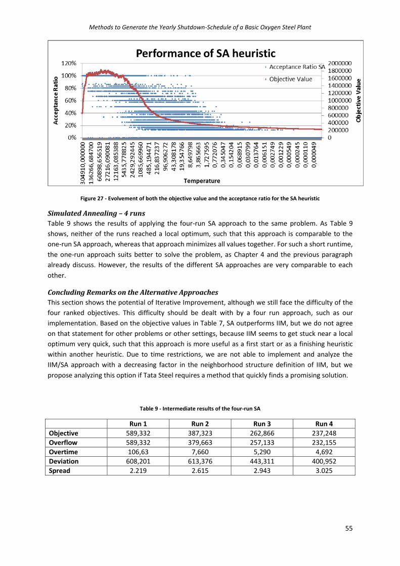
Methods to Generate the Yearly Shutdown-Schedule of a Basic Oxygen Steel Plant
55
Figure 27 - Evolvement of both the objective value and the acceptance ratio for the SA heuristic
Simulated Annealing – 4 runs
Table 9 shows the results of applying the four-run SA approach to the same problem. As Table 9
shows, neither of the runs reached a local optimum, such that this approach is comparable to the
one-run SA approach, whereas that approach minimizes all values together. For such a short runtime,
the one-run approach suits better to solve the problem, as Chapter 4 and the previous paragraph
already discuss. However, the results of the different SA approaches are very comparable to each
other.
Concluding Remarks on the Alternative Approaches
This section shows the potential of Iterative Improvement, although we still face the difficulty of the
four ranked objectives. This difficulty should be dealt with by a four run approach, such as our
implementation. Based on the objective values in Table 7, SA outperforms IIM, but we do not agree
on that statement for other problems or other settings, because IIM seems to get stuck near a local
optimum very quick, such that this approach is more useful as a first start or as a finishing heuristic
within another heuristic. Due to time restrictions, we are not able to implement and analyze the
IIM/SA approach with a decreasing factor in the neighborhood structure definition of IIM, but we
propose analyzing this option if Tata Steel requires a method that quickly finds a promising solution.
Table 9 - Intermediate results of the four-run SA
Run 1 Run 2 Run 3 Run 4
Objective 589,332 387,323 262,866 237,248
Overflow 589,332 379,663 257,133 232,155
Overtime 106,63 7,660 5,290 4,692
Deviation 608,201 613,376 443,311 400,952
Spread 2.219 2.615 2.943 3.025

Methods to Generate the Yearly Shutdown-Schedule of a Basic Oxygen Steel Plant
56
5.3 The Generated YSS Section 5.2.1 already discusses the objective values and the quality of the SA approach. This section
analyzes the rules of thumb in Section 5.3.1 and analyzes the generated clusters in Section 5.3.2.
Finally, Section 5.3.3 compares the generated YSS with the YSS that Tata Steel generated. Due to the
high amount of jobs and periods, we are unable to add the generated YSS, whereas adding a week
based schedule does not make sense for the aim of showing it: the clustering of jobs.
5.3.1 Rules of Thumb and Other Issues in the New Method
This section evaluates every rule of thumb that Section 2.5.2 discusses. Each of the next four sections
discusses one area in the plant and starts with a short repetition of the rules of thumb in that area.
Recall that the SA procedure did not find an optimum yet, such that illogical parts still exist in the
YSS. Furthermore, we reflect on the rules of thumb from an overflow point of view and do not take
any other issues – such as safety issues – into account.
Charging Area
The only rule of thumb for the Charging Area is that outside a plant-shutdown, two installations in
this area may never be down together and the only exception on this rule is that Charging Crane 25
and 26 are allowed to be down together.
The rule should intuitively hold for taking down two installations of the same type (two rozas, pits or
Charging Crane 21 and 25), because in that case no flow through the Charging Area is possible, such
that the optimal schedule does not contain any of these combinations, unless maintenance has to be
performed on for example the power supply. Our YSS does not contain any moment in which two
pits are down together, neither any moment in which the two cranes are down together, but it does
contain eleven periods in which both rozas are down together. However, in none of these eleven
periods the overflow increases, which is mainly due to the fact that these eleven periods are divided
over the year and the maximum adjacent periods that the rozas are down is three periods. These
three periods are scheduled during a plant-shutdown, such that the overflow does not increase.
Figure 28 shows a part of the initial solution with the rozas being down together and the same part
of the generated YSS with the rozas being down together for only two periods. If we manually
reschedule these three jobs back to their initial period in the generated YSS in order to analyze the
result of the move that SA performed, the deviation of the cycle time obviously decreases, but – as
Table 10 shows – the overflow increases. Hence, the SA method obtained a better solution. However,
in the generated YSS there are two hours without any steel, which Tata Steel does not want from a
production point of view and possibly spreading the jobs should be more important for jobs on the
same type of installation (both rozas, both pits) than not deviating from the cycle time.
Table 10 - Result of rescheduling the Rozas
After Change Before Change
Objective 75,433 74,292
Deviation of cycle time 69618 69,622
Buffer Harsco 73,209 72,067
Spread 4.149 4.149
Overtime 2,155 2,155

Methods to Generate the Yearly Shutdown-Schedule of a Basic Oxygen Steel Plant
57
Figure 28 - A part of the initial solution (upper half) and the generated solution (lower half)
Although the pits themselves are not down together and taking down the rozas does not increase the
overflow, the Rijpo requires both pits and the Rofi requires both rozas, such that during performing a
job on the Rijpo or Rofi, the Basic Oxygen Steel Plant cannot process any pig iron. In the input of jobs,
the start moments of these jobs are already equalized, such that the impact on the overflow is the
lowest possible. Still, the SA procedure should schedule these jobs during a plant-shutdown if they
take longer than four hours (Blast-Furnaces produce 770 t/h and the capacity of the hot metal cars
equals 3300). Figure 29 shows the result of performing the jobs on the Rijpo and Rofi outside a plant-
shutdown.
The rule of thumb also applies to installations of a different type. In the generated schedule, for
fifteen times the YSS contains at least one job on more than two installations in the Charging Area.
These fifteen times have a different duration and are not scheduled during a plant-shutdown or
together with the Rijpo or Rofi. In none of these periods there is an overflow of pig iron.
To conclude, performing maintenance on two installations of the same type outside a plant-
shutdown is only possible for less than 4 hours, if the hot metal cars do not contain any iron. Only 1%
of the jobs in the Charging Area require less than 4 hours and in practice the hot metal cars always
contain some pig iron, so we conclude that the rule of thumb holds for performing maintenance on
the same installations. On the other hand, performing jobs on two different installations in the
Charging Area is allowed from an overflow point of view.
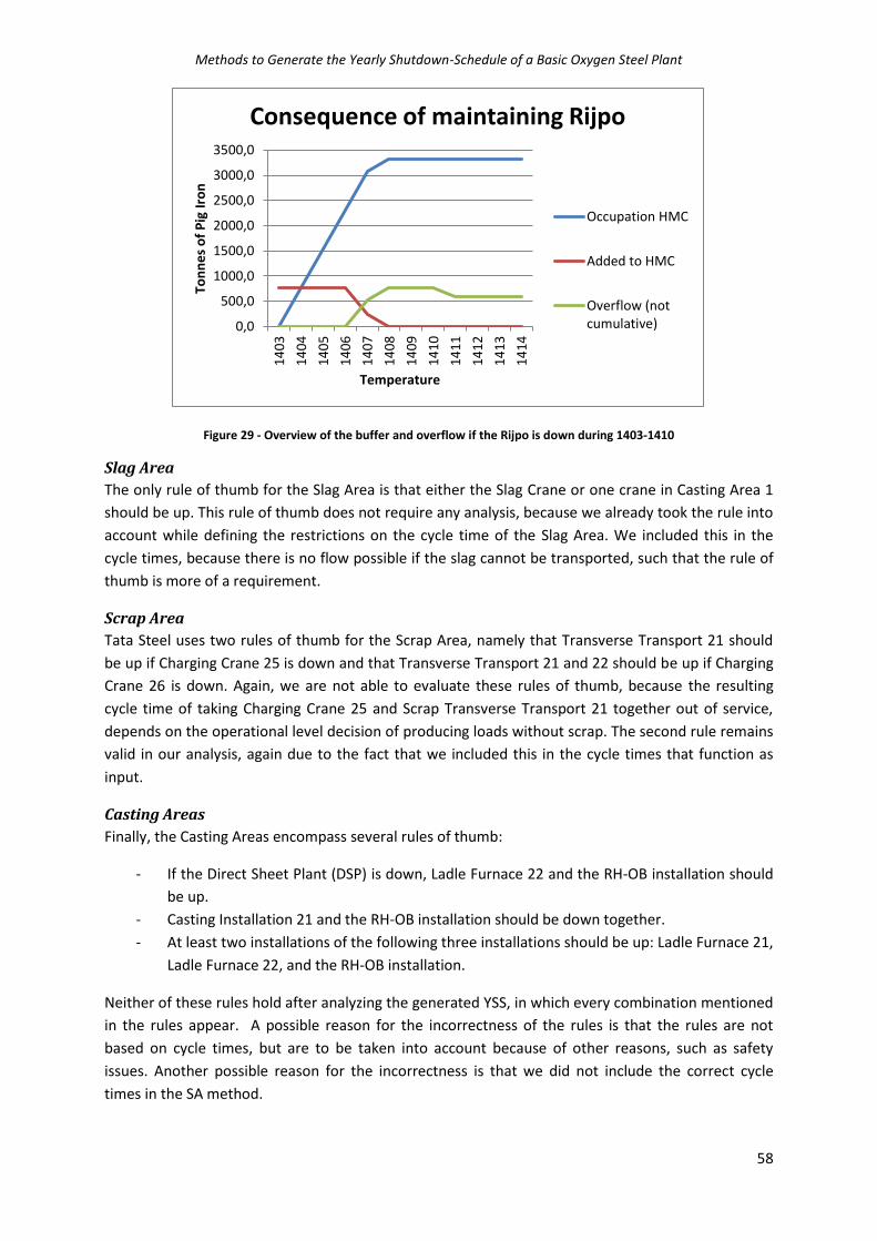
Methods to Generate the Yearly Shutdown-Schedule of a Basic Oxygen Steel Plant
58
Figure 29 - Overview of the buffer and overflow if the Rijpo is down during 1403-1410
Slag Area
The only rule of thumb for the Slag Area is that either the Slag Crane or one crane in Casting Area 1
should be up. This rule of thumb does not require any analysis, because we already took the rule into
account while defining the restrictions on the cycle time of the Slag Area. We included this in the
cycle times, because there is no flow possible if the slag cannot be transported, such that the rule of
thumb is more of a requirement.
Scrap Area
Tata Steel uses two rules of thumb for the Scrap Area, namely that Transverse Transport 21 should
be up if Charging Crane 25 is down and that Transverse Transport 21 and 22 should be up if Charging
Crane 26 is down. Again, we are not able to evaluate these rules of thumb, because the resulting
cycle time of taking Charging Crane 25 and Scrap Transverse Transport 21 together out of service,
depends on the operational level decision of producing loads without scrap. The second rule remains
valid in our analysis, again due to the fact that we included this in the cycle times that function as
input.
Casting Areas
Finally, the Casting Areas encompass several rules of thumb:
- If the Direct Sheet Plant (DSP) is down, Ladle Furnace 22 and the RH-OB installation should
be up.
- Casting Installation 21 and the RH-OB installation should be down together.
- At least two installations of the following three installations should be up: Ladle Furnace 21,
Ladle Furnace 22, and the RH-OB installation.
Neither of these rules hold after analyzing the generated YSS, in which every combination mentioned
in the rules appear. A possible reason for the incorrectness of the rules is that the rules are not
based on cycle times, but are to be taken into account because of other reasons, such as safety
issues. Another possible reason for the incorrectness is that we did not include the correct cycle
times in the SA method.
0,0
500,0
1000,0
1500,0
2000,0
2500,0
3000,0
3500,0
14
03
14
04
14
05
14
06
14
07
14
08
14
09
14
10
14
11
14
12
14
13
14
14
Ton
ne
s o
f P
ig I
ron
Temperature
Consequence of maintaining Rijpo
Occupation HMC
Added to HMC
Overflow (notcumulative)

Methods to Generate the Yearly Shutdown-Schedule of a Basic Oxygen Steel Plant
59
Figure 30 - An overview of clustering installations during a plant-shutdown
Tata Steel can deal with the first possibility by setting the cycle times to 1000 in the input. SA reads
this as if there is no flow through the plant, such that it prevents scheduling these installations
together. Tata Steel can deal with the second possibility by adding the correct cycle times to the
input and finally, there is the possibility that the rules of thumb just do not hold.
Conclusion on the Rules of Thumb
Based on the analysis in this section, we conclude that most rules of thumb do not hold after
analyzing the resulting YSS. However, we admit that the cycle times that function as input may be
incorrect and we recognize that some rules of thumb are to be considered because of other reasons
than overflow. So, we propose to check the cycle times in the input table, to check the reasons for
the rules of thumb, and to reconsider the rules of thumb.
5.3.2 Performance of the Four Objectives
This section analyzes the performance of the SA approach, with respect to the different objectives:
overflow, overtime, deviation from the cycle time, and spreading of jobs. The next sections discusses
these in the mentioned order.
Overflow
As Section 5.2 mentions, none of the runs in the SA procedure reached a local optimum, which is
partly due to the incorrect bounds on the temperature in the first run and due to the short runtime.
However, we are able to search for improvements in the generated YSS’ overflow. The most
important aim is to analyze whether the generated YSS contains intuitively illogical parts.
Figure 30 shows a very high level overview of a cluster of jobs during a plant-shutdown. The figure
shows that the SA procedure did search for the best moments (the vertical axis) to perform
maintenance on critical installations (the horizontal axis). Note that Figure 30 only shows a few
installations and that more than one job can be performed on each of these installations. During this
plant shutdown of 24 hours, 207 jobs are scheduled of which 176 in only ten periods. Such clusters
should contain jobs that require the most critical installations, such as the Rijpo or all cranes in an
area. The cluster in Figure 30 contains at least one job on the Rijpo, Rofi, all charging cranes, both
scrap cranes, the only crane in the Slag Area, both casting installations, and all scrap transverse
transports. Hence, the clustering is intuitively logical.
Figure 31 shows a cluster of jobs that is less intuitively logic, because the DSP and the casting
installations are down together. This means that no steel can be casted, such that the flow through
the plant equals zero. Due to the high duration of the jobs, we expect an overflow somewhere
between period 7596 and 7608. Figure 32 confirms this expectation and shows a red bar at period
7603 until period 7608. However, during these periods, six jobs on Casting Installation 22 are
scheduled and another six jobs that require both casting installations are scheduled, which SA should
reschedule to a better moment one by one.

Methods to Generate the Yearly Shutdown-Schedule of a Basic Oxygen Steel Plant
60
Figure 31 - An illogical part in the generated YSS
SA should finish this rescheduling before the first run ends, as Chapter 4 explains. After the second
run, rescheduling such jobs does not happen anymore, because the tertiary objective always
prevents deviating from the cycle time without improving the overtime or the overflow. Improving
the overflow is impossible with rescheduling one job, because the overflow still exists due to the jobs
left, whereas improving the overtime is possible in this specific part of the schedule. Based on the
possibility to decrease the overtime, we conclude that the SA heuristic just did not have enough time
to consider all these options during the first two runs. However, if the SA heuristic contains the
optimal settings, clusters of installations such as Figure 31 shows are already rescheduled in the first
run. We tried to manually reschedule the whole cluster several times and with every change the
overflow and the objective increased.
Overtime
During 2,155 hours in the generated schedule, maintenance should be performed in overtime, which
is an increase of only 7.75% with respect to the initial schedule in which each job starts at 7am. We
expect that the schedule is near optimal with respect to this objective, because the third and fourth
run still optimized this objective and – due to wrong determination of the minimum difference of the
overflow – this overtime prohibits several changes although the overflow decreases.
This near optimality is supported by the fact that we could not achieve major decreases in the
overtime. On the other hand, we still found jobs in overtime that do not have to be performed in
overtime, which again should be due to the short runtime. An example of reducing the overtime is
moving a job on Casting Installation 22 in Figure 31 to 7am.

Methods to Generate the Yearly Shutdown-Schedule of a Basic Oxygen Steel Plant
61
Figure 32 - Flow of the occupation of Hot Metal Cars and - as a consequence - the moments and amount of the overflow

Methods to Generate the Yearly Shutdown-Schedule of a Basic Oxygen Steel Plant
62
Deviation from the Cycle Time
Clustering jobs leads to deviating from the cycle time, such that – as Table 5 shows – the SA
procedure initially makes the deviation to increase very fast (603,015 in only one run), but after
including this objective in the overall objective, the deviation could still be reduced with 87%.
Nevertheless, the generated YSS seems to be non-optimal with respect to the deviation from the
cycle time as a tertiary objective, because the third run did not reach a local optimum. On the other
hand, this could also be a consequence of not reaching a local optimum in the previous runs.
Spreading of Jobs
We expected that the clustering of jobs would mainly (negatively) influence the spreading of jobs,
which we included in Chapter 4’s model as the standard deviation of the total amount of jobs in a
period. Our analysis of the spread throughout the SA method does not confirm these expectations,
because – as Table 5 – shows, the spread equals 5.03 in the initial solution, whereas it equals 2.757
after the first run. That is exactly the run that should cluster the jobs in order to reduce the overflow.
Apparently, the SA method reschedules jobs to clusters at moments other jobs are not scheduled
yet. As expected, after adding the overtime and the deviation from the cycle time in the objective,
the spread increases, because these aim to schedule the jobs in only 8 hours and on their initial date
– with the high initial standard deviation – respectively. Surprisingly, during the last run (i.e., the only
run that focusses on the spread) the spread keeps increasing and again, the only explanation for this
increase is that the previous runs did not reach a local optimum yet.
Figure 33 shows the division of the jobs over the year. Especially the peak at 2500, the peak at 4220,
and the peak at 7550 stand out. The one in the middle is due to a cluster of 25 jobs on Casting
Installation 22, the one on the left is due to a cluster of 26 jobs on Casting Installation 21, and the
peak on the right is due to 21 jobs on Casting Installation 21. Shutting down a casting installation
increases the cycle time from 18 minutes to 26 minutes and the jobs all require 12 hours, such that
these large clusters are optimal from an overflow point of view. Finally, note that there is a small
peak of 18 jobs in the last period. These jobs are scheduled in the last period, because starting a job
in that period means that it does not finish during the horizon of the YSS and the installation is down
for only one period. In the initial solution, no job is scheduled in the last period, because we added
100 hours to the year.
Figure 33 - Indication of the number of jobs per period
0
5
10
15
20
25
30
35
12
69
53
78
05
10
73
13
41
16
09
18
77
21
45
24
13
26
81
29
49
32
17
34
85
37
53
40
21
42
89
45
57
48
25
50
93
53
61
56
29
58
97
61
65
64
33
67
01
69
69
72
37
75
05
77
73
80
41
83
09
85
77
Am
ou
nt
of
job
s
Period in hours
Total number of jobs per period Number of jobs

Methods to Generate the Yearly Shutdown-Schedule of a Basic Oxygen Steel Plant
63
To circumvent this problem, Tata Steel should just cut-off these 100 hours and reschedule these in
the YSS of the next year. Still, we propose adapting the SA, such that every job finishes in the last
period of the YSS (a year + 100 hours). By means of this adaption, SA will search for a better period
on the YSS, which may be in the last 100 hours, but may also be in the relevant year.
5.3.3 The Generated and the Current YSS
This section compares the YSS of 2013/14 that we generated with the YSS that Tata Steel generated
and uses. We are not able to compare the schedules based on the overtime, deviation from the cycle
time, and the spreading of jobs, because Tata Steel’s YSS solely shows the installations, whereas
these indicators require the specific jobs. Hence, this section solely focusses on the overflow of pig
iron.
Tata Steel’s YSS obtains only 4 times an overflow, of which 3 times are during a plant-shutdown and
which equals to a total overflow of 24,641. Our YSS obtains 23 times an overflow, of which only 3
times during a plant-shutdown and which equals to a total overflow of 72,067. So, our method
generates a YSS that seems to be three times worse than the YSS that the current method generates.
In order to compare the result if we use the same moments for maintaining the (bottleneck) casting
installations, we scheduled these installations in our YSS on the moments Tata Steel schedules these.
We obtained a result of 60,744, which is quite a decrease, but still 2.5 times higher than the overflow
of the current YSS.
The main reason for the gap between the two overflows is in the differences in the bounds on the
start moment of the jobs. We linked the bounds to the priority of a job in SAP, although most of
these priorities are equal to the initial high priority, such that most jobs have a tight bound. We
analyzed whether or not our jobs fit in the YSS as Tata Steel generated it and we conclude that 810 of
the 1483 jobs do not fit to the YSS due to the tight bounds. This 55% difference explains the increase
in moments of overflow in our YSS. Moreover, we did not even include the jobs on highly restricting
installations (e.g., Rijpo, Rofi, all loading cranes, all scrap transverse transports) in these 1483 jobs,
because these are not clearly recognizable in Tata Steel’s YSS.
Another reason for the gap between the overflows in the two schedules may be the long durations in
our YSS, which is also due to the lack of data on the durations in SAP. Again, most entries for the
durations in SAP are empty or equal to zero, such that the shutdown manager had to estimate these
for 644 jobs on 61 installations. We are not able to analyze this reason, because the jobs cannot be
directly linked to a moment in Tata Steel’s YSS, as the previous paragraph explains.
Finally, a reason is the short runtime of the SA procedure, such that it did not obtain a local optimum.
This mainly influences the bad scheduling of the bottleneck casting installations on which 42% of all
jobs have to be performed, as Section 5.4 explains.
5.4 Computation Time Due to the size of the problem space (2287 jobs and on average 1076 possible start moments per
job), the computation time of the program is very high, such that we are not able to perform the
adaptations to the method we propose throughout this chapter. However, we recognize several
possibilities to decrease the runtime, which all aim to decrease the problem size or aim to improve
the local search heuristic. Section 5.2.2 already discusses options to improve the local search
heuristic. This section explains options to decrease the problem size together with the options’
strengths and weaknesses.

Methods to Generate the Yearly Shutdown-Schedule of a Basic Oxygen Steel Plant
64
The problem size is made up of both the number of periods and the number of jobs and this section
discusses possibilities to decrease these vectors. This section first discusses how to decrease the
problem size by decreasing the number of periods and finishes with a discussion on decreasing the
amount of jobs.
An option to decrease the amount of periods is to decrease the days from 24 hours to 16 hours,
which is the longest duration of a job in the current setting. Of course, a job that is not finished at the
end of the day jumps – together with the time – 8 hours. This means that the job finishes the next
morning, even if the job only requires less than 8 hours when the night starts. Such a 33%-decrease
in the amount of periods causes a 33%-decrease in the problem size. However, if a job still requires
only 1 hour when the night starts, the cycle time remains low during the 8-hour-night, although the
job finishes after 1 hour. Hence, this approach does affect the representativeness of the model and
probably has a high impact on the objective value.
Another option to decrease the amount of periods is to decompose the year into semesters or even
quartiles. The main advantage of this decomposition method is that the local search heuristic finds a
local optimum quicker. However, it should find more local optima to capture the whole year. Again,
decomposing the year in smaller periods decreases the optimality of the YSS, but by reconsidering
the last part (e.g., 20%) of the previous YSS and rescheduling these jobs, we expect that the resulting
YSS is rather comparable to the YSS as the current yearly method generates it. Another advantage of
this method is the fact that the current program we built is able to deal with smaller horizons and
that all jobs that have to be performed during the year can still be used as input; the program
recognizes that the job should start after the horizon.
For this research, we already decreased the number of jobs by clustering jobs that clearly belong
together (taking an installation out service, maintaining the installation, put the installation back to
service), but the literature discusses several other options to cluster jobs based on for example the
cycle times (e.g., Van Dijkhuizen and Van Harten (1997) and Gits (1992)). These options are time
consuming and require several additional parameters. Still, we can think of several clusters ourselves
without applying any theory: for the current research we used 122 jobs on Casting Installation 21,
110 jobs on Casting Installation 22, and another 42 jobs that require both casting installations. So,
the jobs on the casting installations count for 42% of the total amount of jobs. Several jobs in these
three sets start at the same moment, have the same duration, and have the same cycle time as
another job in that set, and – as Section 5.3.2 shows – are in a cluster in the generated YSS. As a
consequence, we propose to cluster these jobs. Furthermore, by analyzing previously generated
yearly shutdown-schedules, clusters of jobs that have to be performed together in every schedule
appear. In next years, Tata Steel should use these clusters instead of separate jobs.
These ways to decrease the amount of jobs contradicts with one of the reasons for performing this
research: let the model instead of the user cluster the jobs. On the other hand, some jobs should
definitely form a cluster, such that clustering does not affect the representativeness. We strongly
recommend keep using this way of decreasing the problem size before the heuristic starts, but we
recommend not to cluster the jobs if the jobs do not form an obvious cluster.

Methods to Generate the Yearly Shutdown-Schedule of a Basic Oxygen Steel Plant
65
5.5 Summarizing the Results The four-run SA procedure reduced the objective value of the initial YSS by approximately 89%,
mainly due to the decrease in the overflow. An important disadvantage of the four-run method is the
required local optimum at the end of each run, which our experiment did attain in none of the four
runs. Still, we recognize that the method did solve the problem and generated a YSS in the correct
way, that it influenced the correct objectives, and that it behaved as expected. A major, but easily
preventable, shortcoming of our method is the wrong lower bound on the temperature, such that
the first run did not end in a local optimum. Section 5.2.1 already shows the improved temperatures
and corresponding penalties.
Most rules of thumb as formulated by Tata Steel appear to be unnecessary, although some of these
may have other reasons than just decreasing the overflow. Hence, we recommend reconsidering
these, such that these can either be added to the input of the model, or be left out of the generation
of the YSS.
Although these rules of thumb are not required, the manual method of Tata Steel outperformed our
method on the total overflow during the year. The main reasons for the 65% difference between our
YSS and the current YSS, are the short runtime in our method, the tight bounds on the jobs’ start
moments (55% of the jobs has too tight bounds to fit in the current YSS), and the high durations in
our method.
Our analysis of alternative heuristics to solve the Maintenance Scheduling Problem did neither result
in much better results, nor did these option end up in a local optimum. Moreover, we do not expect
these options to outperform our four-run SA method, although a combination with Iterative
Improvement seems to have a high potential.
Finally, this chapter discussed several options to decrease the problem size by decreasing the
number of periods or the number of jobs. Especially decreasing the number of jobs seems to be
rather promising and can be attained by clustering jobs that have an equal cycle time, an equal
duration, require the same installation, and have the same start date, such as several jobs on the
casting installations.
Methods to Generate the Yearly Shutdown-Schedule of a Basic Oxygen Steel Plant
66
6. Conclusions and Recommendations This chapter covers both the conclusions and the recommendations of this research. First, Section 6.1
contains the conclusions of this research and recommendations based on this research. Section 6.2
contains topics for further research.
6.1 Conclusions This section concludes on our research and explains how we solved the problem of Tata Steel’s Basic
Oxygen Steel Plant with respect to scheduling shutdowns. In Chapter 1 we defined the research
question as: How can the current method of developing the yearly shutdown-schedule at the Basic
Oxygen Steel Plant of Tata Steel be improved, such that the restrictions are met and are clear, and
that all iron produced by the Blast-Furnaces is processed? We answer this question by concluding on
our method in Section 6.1.1. Section 6.1.2 explains the advantages and disadvantages of the method
we propose and Section 6.1.3 covers additional recommendations, which are of direct influence to
the usability of the method.
6.1.1 The Improved Method
Currently, Tata Steel applies a manual method to generate the Yearly Shutdown-Schedule (YSS),
which is based on experience and smart rules of thumb. The literature on the other hand, solely
discusses mathematical and automated methods to solve the Maintenance Scheduling Problem.
Previously performed research solely solves the problem with a single objective, whereas our
approach generates a YSS that aims to meet the following four ranked restrictions:
1. Process as much of the pig iron that the Blast-Furnaces produce as possible.
2. Perform the least jobs as possible in overtime.
3. Deviate the least from the proposed cycle times as possible.
4. Spread the jobs as much as possible.
In order to generate a YSS that complies with these objectives, we modeled the problem in a Mixed-
Integer Programming (MIP) formulation that requires the moment to start a job as decision variable
and uses a penalty for each of the objectives in order to distinguish between the importance of each
objective. We defined the penalties such that there is a strict ranking in the objectives: an objective
can never decrease at the cost of an increase in a higher ranked objective.
Besides the penalties, the MIP requires the duration, the cycle time, and the priority of every job that
has to be performed during the relevant year. We used the MIP to evaluate schedules, which a
Simulated Annealing (SA) procedure generates. The SA procedure first optimizes the primary
objective and if it finds a high quality YSS based on the overflow (i.e., it finds a local optimum), it adds
the secondary objective until it finds a high quality YSS based on both objectives. This process
continues until the SA optimized the YSS on all four objectives. The SA procedure outperformed
three out of the four other local search techniques that we applied and only an SA procedure that
solved the four objectives in parallel slightly outperformed our approach. However, if we dedicate
more time to running the heuristics, our four-run SA will outperform the other heuristics.

Methods to Generate the Yearly Shutdown-Schedule of a Basic Oxygen Steel Plant
67
6.1.2 Advantages and Disadvantage of the Method
Currently, Tata Steel manually generates the YSS based on discussions with the installation engineers
and several rules of thumb. Our method uses an automated approach to create the YSS. Although
the method requires some manual preparation, our automated approach reduces the hours spent on
generating the YSS.
Furthermore, Tata Steel schedules installations instead of jobs, although all jobs are stored in SAP.
Our method uses these jobs to generate the YSS, because these actually have to be performed
throughout the year. By using these jobs, the method is more transparent than the current method
and consequently generates a more transparent schedule. Another advantage of scheduling jobs is
the possibility for the installation engineers to recognize their own jobs in the YSS instead of their
installation, such that the YSS is better understandable. Hence, the installation engineers probably
propose better adaptions. After the proposed adaptions, adapting the YSS also becomes easier and
clearer, because changing the start moment of a job in the schedule becomes easier. The results of
these adaptions become better analyzable, because the KPIs of the YSS after rescheduling a job can
be calculated easily (our implementation contains the possibility to calculate the KPIs based on a
schedule). Tata Steel should use these KPIs to decide whether or not to accept the rescheduling of
the job.
Furthermore, the inclusion of the jobs and the data in SAP that belong to that job (cycle time,
duration, priority, etc.) decreases the subjectivity of the schedule. Still, the installation engineers
define the duration, the cycle time, and the priority of the jobs, such that the method contains some
subjectivity, but the new method circumvents the major part of this subjectivity in the generation of
the schedule. The fact that the YSS is mainly based on the input of the section increases the trust in
the schedule.
By gathering the correct information and including the jobs, not only the scheduling of moments to
shut down the plant becomes faster, more reliable, and more useful, also the scheduling of a
shutdown itself becomes more reliable and more transparent (a heuristic such as project scheduling
requires the same data and increases the quality of the operational schedule).
The main disadvantage of our approach is the requirement to gather data about each and every job,
which is a time consuming and, as a consequence, an expensive task. However, as Section 6.2
discusses, these data can be used to obtain new insights in the process and jobs and can be used to
improve the scheduling during a shutdown. Furthermore, it increases the understanding of the jobs
and the understanding of the process of defining maintenance needs.
6.1.3 Additional Recommendations
Section 6.1.2 discusses several recommendations between the lines, such as the recommendation to
recalculate the KPIs after manually rescheduling a job. This section does not discuss these
recommendations again, but focusses on recommendations that Section 6.1.2 does not discuss.
Currently, most of the required input parameters are incorrect or are lacking in SAP and we
recommend determining the values of especially the duration and the priority on the short term,
because our implementation generates a near optimal schedule that applies to the input. So, if the
input is incorrect, the outcome will be incorrect. Hence, determining the correct durations, cycle
times, and priorities of the jobs is a requirement for using our method. In order to convince the
sections to spend time on determining the correct data, we advise to show the results after

Methods to Generate the Yearly Shutdown-Schedule of a Basic Oxygen Steel Plant
68
Taak A B C D E F
1
2
3
4
5
6
7
8
9 10 Figure 34 - An example of jobs that are scheduled on their bounds
generating a YSS based on different types of input (e.g., bad input values, acceptable input, and
correct input). Especially the lack of the job’s duration and the inaccuracy of the available durations
influence the quality of the YSS that our method generates, because the overflow of pig iron heavily
depends on the (in)correctness of the durations of the jobs. Besides the unavailability of the
durations, the lack of priorities in SAP influences the method in the freedom to schedule clusters in
each other’s shadow: currently every job with a lacking priority has tight bounds on the moment to
be scheduled, whereas several jobs actually have loose bounds instead.
Even if this data is correct, we advise to analyze the jobs that are scheduled close to their bounds,
because these may be right after or right before another cluster of jobs, which is just outside the
bounds of the job, as Figure 34 shows. In Figure 34, A-F are jobs that have to be scheduled during the
periods that correspond to the grey areas (i.e., the grey areas are the bounds of the job). The green
areas show the actual moment that the job is scheduled. Clearly, rescheduling job A, D and E to
period 6 is worth considering. Tata Steel should perform this rescheduling step manually and we
propose to use the KPIs to calculate the quality of the YSS after this rescheduling step, as Section
6.1.2 mentions.
We added 100 hours at the end of the year, such that jobs with an upper bound that reaches over
the YSS’s horizon are allowed to be scheduled after the last period of the year. Note that the jobs
should finish during the last period instead of start during the last period. We advise to keep using
this way of determining the jobs that have to be maintained the next year. Tata Steel should just cut-
off the final part of the schedule and should add these jobs to the input of next year’s YSS.
Finally, we recommend using the Excel-module that indicates the values of the temperatures, based
on the differences between objectives. This module does exactly the same as Chapter 4 explains.
However, we recommend adapting the penalties to make these temperatures unequal. Section 5.2.1
explains the procedure to obtain the penalties and shows which values apply to the current problem.
Note that the penalties may change every year, until the optimal penalties are available, as the final
paragraph of Section 6.2 discusses.

Methods to Generate the Yearly Shutdown-Schedule of a Basic Oxygen Steel Plant
69
6.2 Further Research This chapter sets forth possibilities and requirements for further research and starts with the most
important requirements for further research.
Before applying the model, Tata Steel should determine the correct input data: the cycle times of the
jobs, the priorities of these jobs, and the duration of these jobs. Defining the correct duration of a job
is rather easy, because Tata Steel can easily obtain these data during the upcoming year and improve
it during the subsequent years. The priorities are also rather easy to determine, because the
installation engineers will have this knowledge. Moreover, Tata Steel already puts more effort in
determining these values.
However, engineers may store wrong values to SAP (e.g., a long duration), such that they have more
time to finish their task. In order to deal with these kinds of errors, we propose to perform some
research on the possibility to store the actual durations of the jobs and take yearly averages. Based
on these values, comparisons can be made with the actual performance. There are other ways to
deal with these kinds of errors and we propose performing more research on this subject.
Improving the cycle time of a job is more complex than improving the duration and the priority of a
job. The current cycle times of maintenance are adapted to the cycle times that were used for the
previous yearly shutdown-schedules and Grall et al. (2002) propose an interesting and seemingly
useful model to include the correct cycle times of the jobs. They recognize that the preventive
replacement decision should be jointly optimised with the inspection dates, instead of using these as
input variables. The model they propose schedules predictive maintenance for a detoriating system
and they use continuous time and a continuous state of the system. Their model only focusses on a
single unit, probably because – as they state – “the price for this higher efficiency is the requirement
of a mathematical model for the stochastic deterioration process of the maintained system …
Usually, the task of deriving such a mathematical model is more complicated than just statistically
describing the binary transition from a good state to a failed state”. Additionally, we refer to Duarte
et al. (2006), Sherbrooke (2004), Aven and Jensen (1999), and Gertsbakh (2005) for a discussion on
how to attain the optimal cycle time.
In our opinion, the complexity of the model heavily increases after the addition of these kinds of
stochastic models, but the model definitely becomes more reliable. The increase in reliability is in the
fact that the model is able to calculate the expected costs of in- or decreasing the cycle time. The
increase in complexity is due to the amount of additional parameters that are required, such as the
costs of corrective and preventive maintenance and the mean time to repair. These concepts are
widely discussed in the literature, as Chapter 3 mentions, so adding the correct formulas to the
model will not be too difficult. On the other hand, determining the required input functions requires
a lot of data on for example mean time to repair and mean time to failure. One way to add minimal
complexity, while profiting as much as possible, is to start with adding the complex functions for the
maintenance-bottlenecks.
Additionally, if the cycle times can be expressed in a mathematical function that expresses the costs
of maintenance after delaying it, the model can in- or decrease the cycle times based on these costs.
The current method is not able to deal with these complex functions and equally penalizes every
hour of deviation. A method that uses these functions does not need bounds on maximum deviations
from the cycle time anymore. Still, we expect that the addition of these complex functions to the

Methods to Generate the Yearly Shutdown-Schedule of a Basic Oxygen Steel Plant
70
model does not pay-off the time spend on adding these complex functions. Hence, we propose
defining the optimal cycle times based on these functions and assigning these cycle times to the jobs.
Here another advantage of the method that we propose appears: in the current method of
generating the YSS, it is hard to combine maintenance if every job has a different cycle time. The
automated approach that we propose, deals with these different cycle times as easy as it deals with
equal cycle times. Furthermore, Deshpande and Modak (2002) discuss the result of applying
Reliability Centered Maintenance to a specific installation of a steel plant in India. Their result is that
for several parts of the installation the cycle time of preventive maintenance could be improved from
one month to two months; that is an increase of 100%. Such an increase may also be more cost
efficient at several installations of the Basic Oxygen Steel Plant of Tata Steel. So, there are several
possibilies to improve the determination of the cycle times of the jobs and we advise to perform
more research on this subject, such that the YSS can be optimized.
Chapter 5 recommends on ways to cluster jobs, but for an optimal use of clusters we recommend to
apply models such as Van Dijkhuizen and Van Harten (1997) and Gits (1992) discuss. They discuss
methods that lead to a better clustering of jobs. For these methods, it would pay-off if installations
just show their optimal preventive maintenance cycle time, such that our approach combines these
to an optimimal YSS. With respect to the clustering of jobs, we used in our analysis 122 jobs on
Casting Installation 21, 110 jobs on Casting Installation 22, and another 42 jobs that require both
casting installations and a lot of these jobs have the same duration, cycle times, and priorities.
Hence, we propose clustering the jobs on the casting installations or redefining the jobs on the
casting installations, because the casting installations heavily influences the cycle time through the
plant.
We propose reconsidering the cycle times that belong to taking certain combinations of installations
out of service. Chapter 5 explains that we do not confirm all currently applied rules of thumb, either
because these are not based on the overflow restrictions or because the cycle times behind these
rules of thumb are incorrect. Hence, it requires some further research which rules of thumb to
translate to a cycle time (e.g., based on safety issues) and which rules of thumb to reconsider.
Furthermore, Tata Steel can obtain new rules of thumb from the YSS that the method generates.
These rules can be used for quick decisions and short-term scheduling.
As mentioned before, we recommend to apply our method to reschedule the shutdowns when
additional jobs (e.g., projects) appear during the year. In such cases, rescheduling the shutdowns may
have an impact on the objective value. On the other hand, rescheduling the shutdowns possibly
affects the face validity of the method and the generated YSS, because a major change in the YSS due
to a small change in the requirements of a section is an unintuitive consequence. Hence, we advise
to be careful with adapting the YSS if it does not significantly decrease the objective value (i.e., if it
does not significantly decreae the overflow). A possiblity to adapt the schedule based on only one job
is an Iterative Improvement heuristic that solely takes that specific job into account and starts
searching near the current start moment for a new start moment. We advise to perform more
research on analyzing the robustness of our method and advise to perform more research on the
Iterative Improvement heuristic. If the robustness is high or can easily be improved, Tata Steel can
repeat the scheduling process more often, such there is always a schedule available for the upcoming
year (i.e., a rolling horizon is used).

Methods to Generate the Yearly Shutdown-Schedule of a Basic Oxygen Steel Plant
71
Finally, we used penalties in order to make sure that an objective does not influence a lower ranked
objective. Optimally, these penalties represent the benefit of decreasing an objective at the expense
of increasing another objective and more research is required to correctly determine these penalties.
Additionally, we recommend performing more research on the ranking of the different objectives: is
minimizing the deviation from the cycle time more important than spreading the jobs? This ranking
may lead to periods without any steel, such that another ranking may suit better to the problem.
However, another way to prevent periods without any steel may suit better to the needs of Tata
Steel. These considerations have to be analyzed to correctly define the penalties.

Methods to Generate the Yearly Shutdown-Schedule of a Basic Oxygen Steel Plant
72
Bibliography thefreedictionary. (2013). Retrieved February 2, 2013, from thefreedictionary:
http://www.thefreedictionary.com/stochastic
Aarts, E. H., & Korst, J. (1989). Chapter 1 - Combinatiorial Optimization. In E. H. Aarts, & J. Korst,
Simulated Annealing and Boltzmann Machines (p. ??). Wiley.
Aarts, E. H., Korst, J. H., & van Laarhoven, P. J. (1997). Simulated Annealing. In J. K. Lenstra, Local
Search in Combinatorial Optimization (pp. 91-120). New York: Wiley & Sons Ltd.
Aissani, N., Beldjilal, B., & Trentesaux, D. (2009). Dynamic scheduling of maintenance tasks in the
petroleum industry: A reinforcemen tapproach. Engineering Applications of Artificial
Intelligence 22, 1089–1103.
Aissani, N., Beldjilal, B., & Trentesaux, D. (2009). Dynamic scheduling of maintenance tasks in the
petroleum industry: A reinforcement approach. Engineering Applications of Artificial
Intelligence 22, 1089–1103.
Alkhamis, T. M., & Yellen, J. (1995). Refinery units maintenance scheduling using integer
programming. Applied Mathematical Modelling, Vol. 19, September, 544-549.
Aven, T., & Jensen, U. (1999). Chapter 1 + 2. In Stochatic Models in Reliability (pp. 1-44). New York:
Springer.
Baskar, S., Subbarai, P., Rao, M., & Tamilselvi, S. (2003). Genetic algorithms solution to generator
maintenance scheduling with modified genetic operators. IEEE Proceedings-Generation,
Transmission and Distribution, Vol. 150, No. 1, 56-60.
Benders, J. F. (1962). Partitioning Procedures for solving mixed-variable linear programming
problems. Numerische Matematik, 238-252.
Berrichi, A., Yalaoui, F., Amodeo, L., & Mezghiche, M. (2010). Bi-Objective Ant Colony Optimization
approach to optimize production and maintenance scheduling. Computers & Operations
Research, 1584–1596.
Blok, J., Castelijn, P., Hoekstra, S., & Kokkeler, F. (2012). Scope Management of Shutdowns -
Invloedsfactoren & Strategieen. Enschede: Universiteit Twente.
Budai, G., Huisman, D., & Dekker, R. (2004). Scheduling Preventive Railway Maintenance Activities.
Econometric Institute Report EI 2004-41, 1-15.
Burke, E. K., & Smith, A. J. (2000). Hybrid Evolutionary Techniques for the Maintenance Scheduling
Problem. IEEE Transactions on Power Systems, Vol. 15, 122-128.
Burke, E. K., Clark, J. A., & Smith, A. J. (1997). Four Methods for Maintenance Scheduling. Proceedings
of the International Conference on Artificial Neural Networks and Genetic Algorithms, 264–
269.
Chattopadhyay, D. (1998). A Practical Maintenance Scheduling Program: Mathematical Model and
Case-Study. IEEE Transactions on Power Systems, Vol 13, No. 4, 1475-1480.

Methods to Generate the Yearly Shutdown-Schedule of a Basic Oxygen Steel Plant
73
Chattopadhyay, D., Bhattacharya, K., & Parikh, J. (1995). A Systems Approach to Least-Cost
Maintenance Scheduling for an Interconnected Power System. IEEE Transactions on Power
Systems, Vol. 10, No. 4, 2002-2007.
Coley, D. A. (1999). An Introduction to Genetic Algorithms for Scientists and Engineers. Singapore:
World Scientific Publishing Co. Pte. Ltd.
Dahal, K. P., & Chakpitak, N. (2007). Generator maintenance scheduling in power systems using
metaheuristic-based hybrid approaches. Electric Power Systems Research 77, 771–779.
Dahal, K. P., Aldridge, C., & McDonald, J. (1999). Generator maintenance scheduling using a genetic
algorithm with a fuzzy evaluation function. Fuzzy Sets and Systems 102, 21-29.
Dekker, R. (1996). Applications of maintenance optimization models: a review and analysis. Reliability
Engineering and System Safety 51, 229-240.
Deshpande, V. S., & Modak, J. P. (2002). Application of RCM for safety considerations in a steel plant.
Reliability Engineering and System Safety 78, 325–334.
Dopazo, J. F., & Merrill, H. M. (1975). Optimal Generator Maintenance Scheduling Using Integer
Programming. IEEE Transactions on Power Apparatus and Systems, Vol. PAS-94, no. 5, 1573-
1545.
El Moudan, W., & Mora-Camino, F. (200). A dynamic approach for aircraft assignment and
maintenance scheduling by airlines. Journal of Air Transport Management 6, 233-237.
El-Amin, I., Duffuaa, S., & Abbas, M. (2000). A Tabu search algorithm for maintenance scheduling of
generating units. Electric Power Systems Research 54, 91–99.
El-Sharkh, M. Y., & El-Keib, A. A. (2003). An evolutionary programming-based solution methodology
for power generation and transmission maintenance scheduling. Electric Power Systems
Research 65, 35-40.
Escudero, L. F. (1982). On maintenance scheduling of production units . European Journal of
Operational Research 9, 264-274.
Fetanat, A., & Shafipour, G. (2011). Generation maintenance scheduling in power systems using ant
colony optimization for continuous domains based 0–1 integer programming. Expert Systems
with Applications 38, 9729–9735.
Gertsbakh, I. (2005). Preventive Maintenance Models Based on the Lifetime Distribution. In
Reliability Theory with Applicants to Preventive Maintenance (pp. 67-102). Berlin: Springer.
Gits, C. W. (1992). Design of Maintenance Concepts. International Journal of Production Economics,
24, 217-226.
Glover, F., Taillard, E., & de Werra, D. (1993). A user's guide to tabu search. Annals of Operations
Research 41, 3-28.
Gopalakrishnan, M., Mohan, S., & He, Z. (2001). A tabu search heuristic for preventive maintenance
scheduling. Computers and Industrial Engineering 40, 149-160.

Methods to Generate the Yearly Shutdown-Schedule of a Basic Oxygen Steel Plant
74
Grall, A., Dieulle, L., & Béreng, C. (2002). Continuous-Time Predictive-Maintenance Scheduling for a
Deteriorating System. IEEE Transactions on Reliability, Vol. 51, No. 2, 141-150.
Heerkens, H. (2004). Managerial Problem-Solving Method.
Hertz, A., Taillard, E., & de Werra, D. (2003). Chapter 5, Tabu Search. In E. Aarts, & K. Lenstra, Local
Search in combinatorial optimization (pp. 121-136). Oxfordshire: Princeton University Press.
Holland, J. H. (1992). Genetic Alghorithms. Scientific American, 66-72.
Huang, C. J., Lin, C. E., & Huang, C. E. (1992). Fuzzy approach for generator maintenance scheduling .
Electric Power Systems Research, 24, 31-38.
Huang, C. J., Lin, C. E., & Huang, C. E. (1992). Fuzzy approach for generator maintenance scheduling.
Electric Power Systems Research, 24, 31-38.
Huang, S.-J. (1998 ). A genetic-evolved fuzzy system for maintenance scheduling of generating units.
lectrical Power & Energy Systems, Vol. 20, No. 3, 191-195.
Inuiguchi, M., & Ramík, J. (2000). Possibilistic linear programming: a brief review of fuzzy
mathematical programming and a comparison with stochastic programming in portfolio
selection problem. Fuzzy Sets and Systems 111, 3-28.
Kirkpatrick, S., Gelatt, C. D., & Vecchi, M. P. (1983). Optimization by Simulated Annealing. Science,
New Series, Vol. 220, No. 4598, 671-680.
Kralj, B. L., & Petrović, R. (1988). Optimal preventive maintenance scheduling of thermal generating
units in power systems - A survey of problem formulations and solution methods. European
Journal of Operational Research 35, 1-15.
Kralj, B., & Petrovic, R. (1995). A multiobjective optimization approach to thermal generating units
maintenance scheduling. European Journal of Operational Research 84, 481-493.
Lima, R. M., Grossmann, I. E., & Jiao, Y. (2011). Long-term scheduling of a single-unit multi-product
continuous process to manufacture high performance glass. Computers and Chemical
Engineering 35, 554–574.
Marwali, M. K., & Shahidehpour , S. M. (1998). Integrated generation and transmission maintenance
scheduling with network constraints. IEEETransactions on Power Systems, Vol.13, No.3, 1063-
1068.
Metropolis, N., Rosenbluth, A. W., Rosenbluth, M. N., Teller, A. H., & Teller, E. (1953). Equation of
State Calculations by Fast Computing Machines. The Journal of Chemical Physics, vol. 21, no.
6, 1087-1092.
Moghaddam, K. S. (2008). Preventive Maintenance and Replacement Scheduling: Models and
Algorithms. Lousivile: University of Louisville.
Mohanta, D. K., Sadhu, P. K., & Chakrabarti, R. (2007). Deterministic and stochastic approach for
safety and reliability optimization of captive power plant maintenance scheduling using

Methods to Generate the Yearly Shutdown-Schedule of a Basic Oxygen Steel Plant
75
GA/SA-based hybrid techniques: A comparison of results. Reliability Engineering and System
Safety 92, 187–199.
Muckstadt, J. A., & Wilson, R. C. (1968). An Application of Mixed-Integer Programming Duality to
Scheduling Thermal Generating Systems. IEEE Transactions on Power Apparatus and Systems,
1968-1978.
Peng, F., Kang, S., Li, X., Ouya, Y., Somani, K., & Acharya, D. (2011). A Heuristic Approach to the
Railroad Track Maintenance Scheduling Problem. Computer-Aided Civil and Infrastructure
Engineering 26, 129–145.
Perquin, S. (2005). Cargo Nieuws Pagina. Retrieved April 12, 2013, from Rolandrail.net:
www.rolandrail.net/nieuws/fotopag_00676.htm
Pinedo, M. L. (2009). Planning and Scheduling in Manufacturing and Services 2nd edition. New York:
Springer.
Ruiz, R., García-Díaz, J. C., & Maroto, C. (2007). Considering scheduling and preventive maintenance
in the flowshop sequencing problem. Computers & Operations Research 34, 3314 – 3330.
Saraiva, J. T., Pereira, M. L., Mendes, V. T., & Sousa, J. C. (2011). A Simulated Annealing based
approach to solve the generator maintenance scheduling problem. Electric Power Systems
Research 81, 1283–1291.
Satoh, T., & Nara, K. (1991). Maintenance Scheduling By Using Simulated Annealing Method. IEEE
Power Engineering Society, 859-857.
Sherbrooke, C. C. (2004). Optimal Inventory Modeling of Systems, 2nd edition. Boston: Kluwer
Academic Publishers.
Slack, N., Chambers, S., & Johnston, R. (2007). Operations Management. Essex: Pearson Education
Limited.
Soh, S. S., Nor, R. H., & Haron, H. (2012 ). Review on Scheduling Techniques of Preventive
Maintenance Activities of Railway. Fourth International Conference on Computational
Intelligence, Modelling and Simulation. IEEE Computer Society.
Suresh, K., & Kumarappan, N. (2012). Hybrid Improved Binary Particle Swarm Optimization Approach
for Generation Maintenance Scheduling Problem. Swarm and Evolutionary Computation,
Article in Press.
Umiliacchi, P., Lane, D., & Romano, F. (2011). redictive maintenance of Railway Subsystems Using An
Ontology Based Modelling Approach. 9th World Conference on Railway Research, (pp. 1-10).
Lille, France.
Van Dijkhuizen, G., & Van Harten, A. (1997). Reliability Theory with Applicants to Preventive
Maintenance. European Journal of Operational Reserach 99, 552-564.
Volkanovski, A., Mavko, B., Boševski, T., Čauševski, A., & Čepin, M. (2008). Genetic algorithm
optimisation of the maintenance scheduling of generating units in a power system. Reliability
Engineering and System Safety 93, 757–767.

Methods to Generate the Yearly Shutdown-Schedule of a Basic Oxygen Steel Plant
76
Wang, Y., & Handschin, E. (2000). A new genetic algorithm for preventive unit maintenance
scheduling of power systems. Electrical Power and Energy Systems 22, 343–348.
Winston, W. L. (2004). Operations Research - applications and algorithms 4th edition. Belmont:
Thomson Learning.
Yamayee, Z. A. (1982). Maintenance Scheudling: Description, Literature Survey, and Intervace with
Overall Operations Scheduling. IEEE Transactions on Power Apparatus and Systems, Vol. PAS-
101, No. 8, 2270-2279.
Zürn, H. H., & Quintana, V. (1975). Generator Maintenance Scheduling Via Successive Approximations
Dynamic Programming. IEEE Transactions on Power Apparatus and Systems, vol. PAS-94, no.
2, 665-671.

Methods to Generate the Yearly Shutdown-Schedule of a Basic Oxygen Steel Plant
77
Appendices
A Translation of Terms This appendix contains a translation of several terms used throughout the report. This appendix only
contains the translation from English to Dutch.
B
basic oxygen steel plant oxystaalfabriek
blast-furnace hoogoven
C
casting crane gietkraan
casting installation gietinstallatie
charging crane laadkraan
converter converter
D
dust exhaustion stofafzuiging
E
exhaust fan afzuigventilator
exhaust system afzuiginstallatie
H
hot metal car ruwijzer menger
hot strip mill warmbandwals
G
gantry crane bovenloop kraan
L
ladle furnace panoven
ladle transport (car, wagon) dwarstransportwagen
ladle transport VPBI dwarstransport VPBI
loading crane laadkraan
O
overhead travelling crane bovenloopkraan
P
pit put
pig iron ruwijzer
R
refractory vuurvast
raw iron desulphizer installation (ROZA) ruw ijzer ontzwavelings installatie (ROZA)
RH-OB installation vacuüumpanbehandelingsinstallatie (VPBI)

Methods to Generate the Yearly Shutdown-Schedule of a Basic Oxygen Steel Plant
78
S
scrap schrot
slab area plakkenhal
slag slak
stirring station spoelstand
semi portal halfportaal kraan
T
transverse transport dwarstransport

Methods to Generate the Yearly Shutdown-Schedule of a Basic Oxygen Steel Plant
79
B Maps the Basic Oxygen Steel Plant and the IJmuiden Site This appendix includes a map of the IJmuiden Tata Steel Site (B.1) and the Basic Oxygen Steel Plant
(B.2). Please combine these maps with the flowchart in Figure 5, which indicates the different flows
of iron, steel, slag, and scrap through the plant.
B.1 IJmuiden Tata Steel Site

Methods to Generate the Yearly Shutdown-Schedule of a Basic Oxygen Steel Plant
80
B.2 Map of the Basic Oxygen Steel Plant

Methods to Generate the Yearly Shutdown-Schedule of a Basic Oxygen Steel Plant
81
C Defining the Minimum and Maximum Differences between
Neighboring Solutions To define the minimum and maximum difference between two solutions, we analyze the maximum
difference per part of the total objective value.
Overflow
A rescheduling-move can make the capacity of the Basic Oxygen Steel Plant to decrease from 933.33
tonnes per hour (cycle time is 18 minutes, load of 280 tonnes) to 0 t/h. However, the overflow can
only increase with 770 t/h, because the Blast-Furnaces produce at most 770 t/h. The maximum
duration of a job that is able to influence the cycle time from optimality to infinity is 8 hours and
hence the maximum difference in overflow due to one move corresponds to .
Notice that other jobs take more than 8 hours, but these jobs only influence the cycle time if a
certain set of other combination is also down. In these cases, the required set of installations already
influences the cycle time such that the new schedule’s overflow does not reach an increase of 6160 t.
The minimum increase in the overflow equals to 68 tonnes, which corresponds to an increase of one
minute in the cycle time for one hour.
Overtime
The maximum increase in overtime equals to 8 hours, because only the hours that were performed
during the day in the previous schedule can be additional overtime in the neighboring schedule.
The minimum increase in the overtime equals to one hour.
Deviation from the Cycle Time
The maximum increase in deviating from the cycle time equals to 1680 hours (10 weeks) and the
minimum increase in the deviation from the cycle time equals to 1 hour.
Spread
The maximum difference in the standard deviation is about 0.15, due to high amount of periods
(8836) we consider and the small changes in the values in these periods – at most 32 of these periods
change with one point.
The minimum difference is approximately 0.01, if one job changes when the previous standard
deviation equals to 0.
Penalties
The different objectives require a strict ranking. Hence, if there is a decrease in the overflow value,
this decrease should always be more than an increase in any other objective. Hence, we set the
penalties for overflow, overtime, deviation from the cycle time, and spreading of jobs equal to 1, 1,
0.001, and 0.001 respectively.
Conclusion
Based on the differences between the partly objectives and the penalties, the maximum difference
of the total objective value equals to 6160 + 8 + 1680/1000 + 0.15/1000 = 6184.95 and the minimum
difference equals to 0 + 0 + 0 + 0.01/1000 = 0.00001.