Methods of solving problems in electrostatics

Section 3

Method of Images

• Plane interface between a semi-infinite (hence grounded) conductor and vacuum

Find fictitious point charges, which together with given charges, make the conductor surface an equipotential (f = 0)

Df = 0 satisfied. Boundary conditions satisfied. Uniqueness theorem. Done.

Vanishes on boundary, when r’ = r

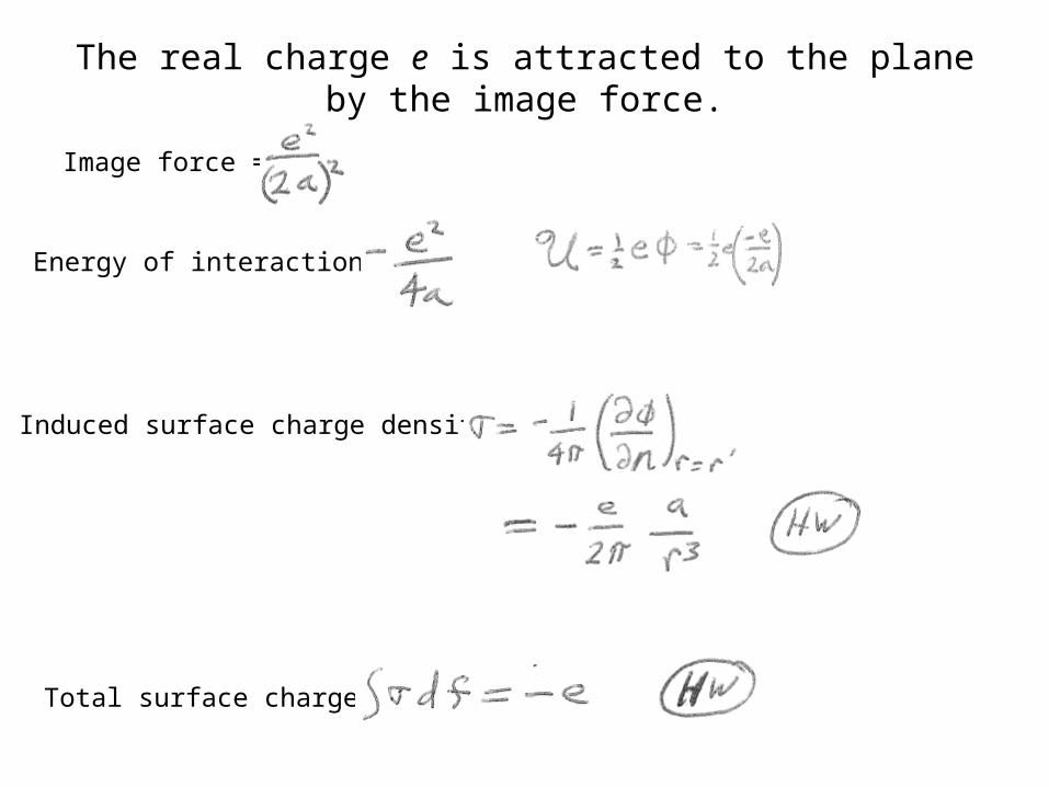
The real charge e is attracted to the plane by the image force.

Image force =

Energy of interaction =

Induced surface charge density =

Total surface charge =

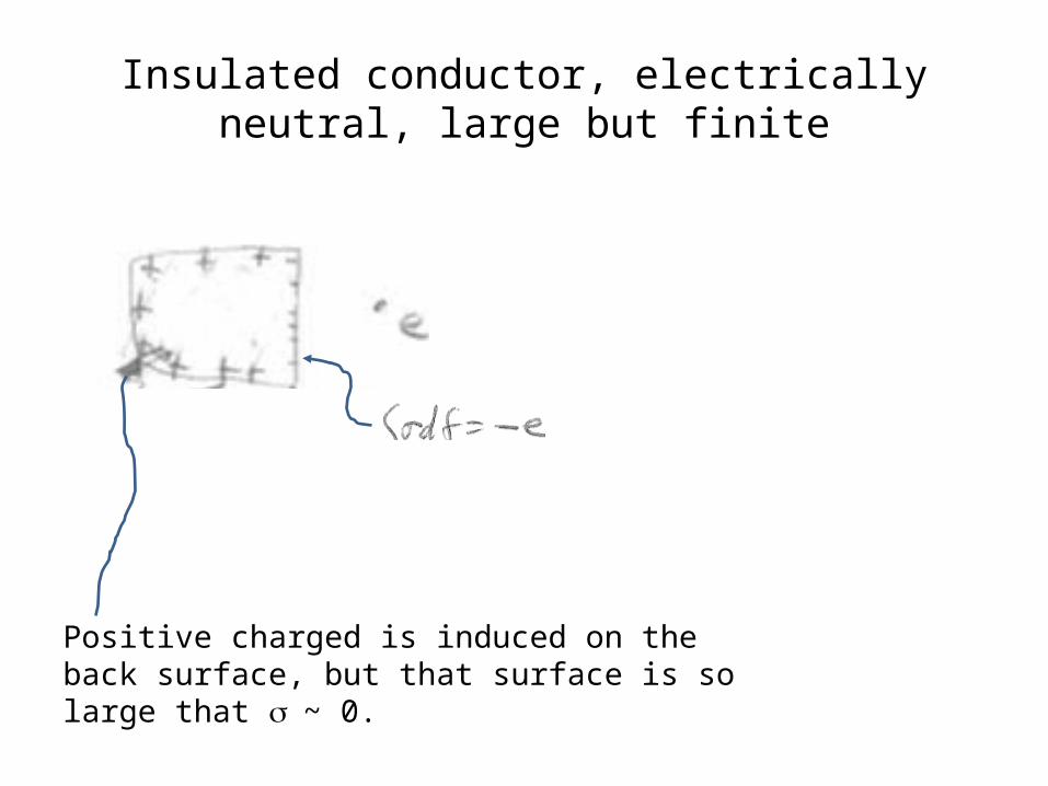
Insulated conductor, electrically neutral, large but finite

Positive charged is induced on the back surface, but that surface is so large that s ~ 0.

Spherical conductorField point P(x,y,z)

In the space outside the sphere

f vanishes on the surface if l/l’ = (e/e’)2 and R2 = l l’ (HW)

eActual charge

Fictitious image charge

If spherical conductor is grounded, f = 0 on the surface.

Potential outside the sphere is

since

Induced charge on the surface is

= e R/l

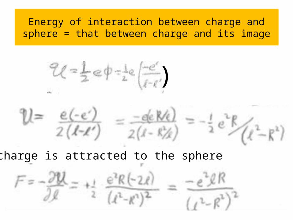
Energy of interaction between charge and sphere = that between charge and its image

)

The charge is attracted to the sphere

If the conducting sphere is insulated and uncharged, instead of grounded, it has nonzero constant potential on surface.

Then we need a 2nd image charge at the center = +e’

Interaction energy of a charge with an insulated uncharged conducting sphere

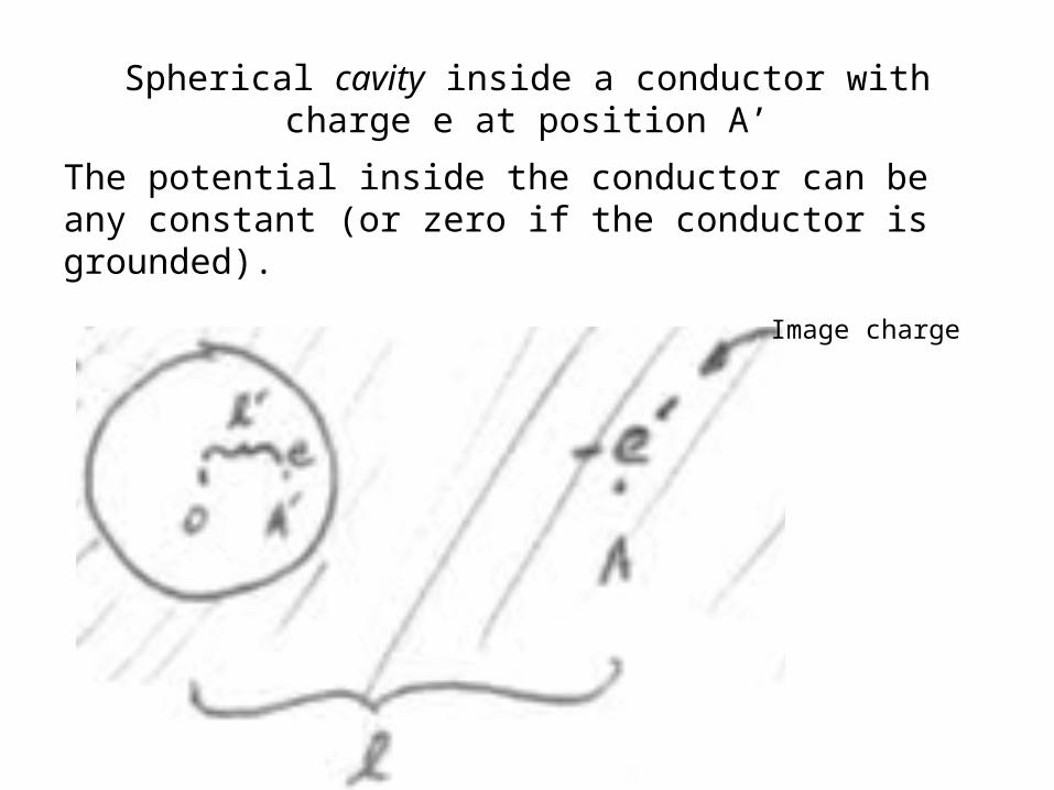
Spherical cavity inside a conductor with charge e at position A’

The potential inside the conductor can be any constant (or zero if the conductor is grounded).

Image charge

Field inside cavity is determined by this part, independent of the constant.

The potential on the inner surface of the cavity must be the same constant: Boundary condition

-e’=eR/l’

Potential at the cavity field point P

Vanishes on the boundary

The total potential is

Method of Inversion

Laplace’s equation in spherical coordinates

This equation is unaltered by the inversion transform r -> r’ where r = R2/r’, while f -> f’ with f = r’ f’/R.R is the “radius of the inversion”

Consider a system of conductors, all at f0, and point charges.

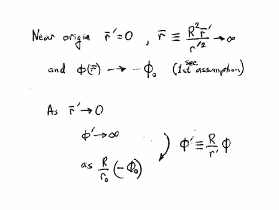
• Usually f->0 as r-> infinity• Shift zero of potential so that conductors are at zero potential

and f -> - f0 as r -> infinity• What problem is solved by f’?

• Inversion changes the shapes and positions of all conductors. – Boundary conditions on surfaces unchanged, since if f = 0,

then f’ = 0, too.

• Positions and magnitudes of point charges will change.– What is e’?

f=0

inversion

|2

r - r0

As r (the field point) approaches r0 (the charge point)

But f’

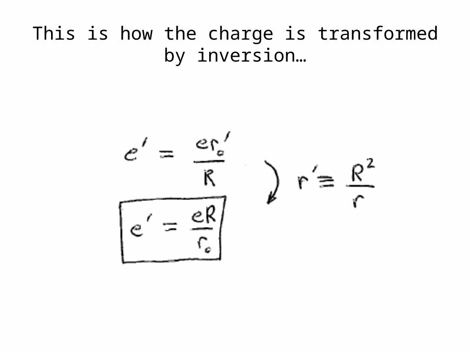
This is how the charge is transformed by inversion…

Inversion transforms point charges, moves and changes shapes of conductors, and puts a new charge at the origin. Why do it?

In the inverted universe, there is a charge

After inversion, the equation of the sphere becomes

Equation of the sphere

Another sphere

Spherical conductors are transformed by inversion into new spherical conductors

If the original sphere passes through the origin

This sphere is transformed into a plane

from the originAnd distant

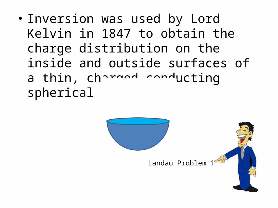
• Inversion was used by Lord Kelvin in 1847 to obtain the charge distribution on the inside and outside surfaces of a thin, charged conducting spherical bowl.

Landau Problem 10

Method of Conformal Mapping

2D problem of fields that depend on only two coordinates (x,y) and lie in (x,y) plane

Electrostatic field:

Vacuum:

A vector potential for the E-field (not the usual one)

Then w(z) has a definite derivative at every point independent of the direction of the derivative

Derivatives of w(z) = f(z) – i A(z) in complex plane, z = x + iy

Take derivative in the x-direction

w is the “complex potential”

Ex

Ey

Lines where Im(w) = constant are the field lines

Lines where Re(w) = f = constant are equipotentials

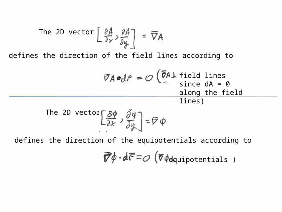
The 2D vector

defines the direction of the field lines according to

field lines since dA = 0 along the field lines)

The 2D vector

defines the direction of the equipotentials according to

equipotentials )

Equipotentials and field lines are orthogonal.

Since

Electric flux through an equipotential line

n = direction normal to dl

We have

Direction of dl is to the left when looking along n

n

X

f decreasing in the x directionA increasing in the y direction

f decreasing in the y directionA decreasing in the x direction

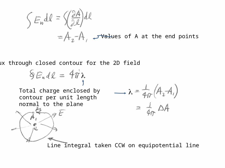
Values of A at the end points

Flux through closed contour for the 2D field

Total charge enclosed by contour per unit length normal to the plane

l

l

Line integral taken CCW on equipotential line

Trivial example: What is the field of a charged straight wire?

cylinder

l = charge per unit length

Solution using complex potential

then Integral around circle

Solution using Gauss’s law

w = w(z) is the conformal map of the complex plane of z onto the complex plane of w

Cross section C of a conductor that is translationally invariant out of plane.

Potential f = f0 is constant on C

The method maps C onto line w = f0

Then Re[w] = f at points away from C.

x

= x + iy