1

METHODS FOR MAPPING BETWEEN THE EQ-5D-5L AND THE 3L

FOR TECHNOLOGY APPRAISAL

REPORT BY THE DECISION SUPPORT UNIT

11th July 2017

Monica Hernandez Alava, Allan Wailoo, Stephen Pudney

Health Economics and Decision Science, School of Health and Related Research, University of

Sheffield, UK

Decision Support Unit, ScHARR, University of Sheffield, Regent Court, 30 Regent Street Sheffield, S1 4DA Tel (+44) (0)114 222 0734 E-mail dsuadmin@sheffield.ac.uk Website http://scharr.dept.shef.ac.uk/nicedsu/ Twitter @NICE_DSU

2

ABOUT THE DECISION SUPPORT UNIT The Decision Support Unit (DSU) is based at the School of Health and Related Research, University

of Sheffield and is commissioned by the National Institute for Health and Care Excellence (NICE) to

provide a research and training resource to support the Institute's Technology Appraisal Programme.

Please see our website for further information http://scharr.dept.shef.ac.uk/nicedsu/

Disclaimer The production of this document was funded by NICE through its Decision Support Unit. The views,

and any errors or omissions, expressed in this document are of the authors only. NICE may take

account of part or all of this document if it considers it appropriate, but it is not bound to do so.

Acknowledgements We would like to thank Professor Andrew Jones (University of York) and Professor David Zimmer

(Western Kentucky University) who provided peer review of this report and underlying analyses. We

are also grateful to Rosie Lovett (NICE) for helpful comments on previous drafts.

3

EXECUTIVE SUMMARY Background

EQ-5D comprises a descriptive system and a set of values for each health state that can be

described. The descriptive system allows respondents to indicate their health state on five

dimensions of health: mobility, ability to self-care, ability to undertake usual activities, pain

and discomfort, and anxiety and depression. In the 3-level version (3L), respondents indicate

the degree of impairment on each dimension according to three levels (no problems, some

problems, extreme problems). A new, five-level version (5L) includes five levels of severity

for each dimension (no problems, slight problems, moderate problems, severe problems, and

extreme problems).

Previous work by the DSU has demonstrated that there are substantial differences between

the way in which 3L and 5L estimate gains for health technologies in terms of Quality

Adjusted Life Years (QALYs) and, in turn, their cost-effectiveness. These differences occur

both in terms of the responses individuals give to the two descriptive systems and the

valuation of health states. This means that consistent decisions can only be made if NICE

recommends one or other of the instruments. Whichever is recommended, there will be

evidence generated in 3L and 5L that forms part of NICE appraisals for many years to come.

This report describes and assesses different options for linking evidence (“mapping”) from

3L to 5L and vice versa. The ability for analysts to do this in a robust and consistent manner

is required for NICE to issue guidance that is based on a coherent assessment of available

evidence.

Available options

The DSU has developed and described a statistical method for mapping between 3L and 5L,

in either direction. The method has been estimated using two different datasets: a EuroQoL

dataset (EQG, n=3691) and a National Data Bank for Rheumatic Diseases dataset (NDB,

n=5,311). The two DSU models can be used not only to estimate a utility score for one

instrument (3L or 5L) from responses to the descriptive system of the other, but can also

estimate a utility score for one instrument (3L or 5L) from a utility score of the other. The

utility score that is being mapped from does not have to be a value that corresponds to a

4

particular health state in the descriptive system. It can, for example, represent the mean from

a number of patient responses.

van Hout et al estimate 3L from 5L responses using a series of cross-tabulations of responses

to the 3L and the 5L for each dimension of health, separately. The approach is based on the

same EQG dataset as the DSU approach, but not all the data is used. Responses to the five

domains making up each 3L/ 5L paired response are designated as “inconsistent” or

“consistent”. “Inconsistent” domain responses are treated as missing.

For those situations where the requirement is to map from 3L to 5L, or to map from 5L utility

scores to 3L, the two DSU methods are appropriate. Where the requirement is to map from

5L descriptive system data to 3L utility values, there are three options: the two DSU models

and the van Hout et al approach.

Comparing mapping approaches

We compared model predictions to observed data in the two EQG and NDB datasets.

Mapping from the descriptive system of the 5L to the 3L using the EQG dataset is a within

sample validation for the van Hout and DSU EQG methods. We found few differences

between these two methods and that they largely performed better than the DSU NDB model,

for which this is out-of-sample testing. The DSU EQG model performs slightly better than

the van Hout method in predicting the responses to the 3L descriptive system. Summary

measures of fit to the 3L utility scores slightly favour the van Hout method.

Mapping from the descriptive system of the 5L to the 3L using the NDB dataset showed that

the DSU NDB method very closely aligned to the data. There were not large differences in

terms of overall fit, either to the response probabilities or the 3L utility scores when

comparing the van Hout and DSU EQG methods.

Further investigation demonstrates how standard summary measures of fit are not measuring

the same concept, can be contradictory and that differences between the DSU and van Hout

methods are masked by such measures. The process of adjusting data in the van Hout method

5

artificially reduces the error for parts of responses that conform to the defined “consistency”

criteria, but at the expense of poorer fit for those that do not.

We also show how the two DSU mapping approaches that permit mapping from 3L to 5L

perform exceedingly well in and out of sample.

Discussion and recommendations

For mapping from 3L to 5L, or for mapping from 5L utility values to 3L, there are two

currently available options: the DSU EQG or DSU NDB methods. Both of these methods

demonstrate very close in-sample fit when mapping from 3L to 5L. Furthermore, there are no

significant concerns identified from out-of-sample testing, and biases often seen in mapping

studies more generally are not present in the DSU approach (namely the tendency for simple

methods to overestimate utility for those in relatively poor health and underestimate it for

those in good health). There is little in the analyses we have performed to warrant a

preference for one approach over another.

The DSU and van Hout approaches, for mapping from the 5L descriptive system to 3L, do

not perform substantially differently from each other when assessed using standard measures

of summary fit across the entire data. The DSU approach slightly outperforms van Hout in

terms of predicting the category of response. The van Hout method is marginally better for

some measures of summary fit to utility scores. However, we outline how these summary

measures mask differences between the approaches in different parts of the health

distribution. There are concerns about the validity of the pairwise deletion method employed

by van Hout et al and how this distorts fit measures.

All of the models we have compared are limited by the available data. Both the EQG and

NDB datasets have limitations for the purpose of mapping between 3L and 5L. They are

unlikely to be sufficiently large. Given the potential importance of consistent, robust mapping

methods, we consider it essential that a well-designed, large-scale new data collection

exercise be undertaken in order to estimate a definitive mapping that can be used for decision

making in the UK NHS.

6

CONTENTS EXECUTIVE SUMMARY ..................................................................................................... 3 1. INTRODUCTION............................................................................................................ 7 2. DATA AND METHODS ............................................................................................... 10

2.1. DATA ........................................................................................................................ 10 2.1.1. EuroQoL Group coordinated study (EQG) ....................................................... 10 2.1.2. The NDB dataset ................................................................................................ 10

2.2. METHODS ................................................................................................................. 11 2.2.1. The DSU approach ............................................................................................ 11 2.2.2. The van Hout et al approach ............................................................................. 12

2.3. COMPARISONS OF MAPPING APPROACHES ................................................................. 14 3. COMPARISON RESULTS........................................................................................... 15

3.1. 5L TO 3L: EQG DATASET ......................................................................................... 15 3.2. 5L TO 3L: NDB DATASET ......................................................................................... 22 3.3. ADDITIONAL COMPARISONS OF 5L TO 3L. ................................................................. 27 3.4. 3L TO 5L ................................................................................................................... 29

4. DISCUSSION AND RECOMMENDATIONS............................................................ 31 5. CONCLUSIONS ............................................................................................................ 33 6. REFERENCES ............................................................................................................... 34

----------------------------------------------------------------------------------------------------------------

TABLES Table 1: Options for linking 3L and 5L ................................................................................................................... 8 Table 2: Crosstab of feasible responses to 3L and 5L, within each health dimension .......................................... 12 Table 3: Number of inconsistencies in the EQG dataset ....................................................................................... 13 Table 4: Crosstab of 3L 5L within dimension responses showing those informed by real data in van Hout et al 13 Table 5: Responses considered inconsistent in the van Hout et al mapping ......................................................... 14 Table 6: Overall fit in the EQG dataset ................................................................................................................. 17 Table 7: Ranking of model fit compared with the EQG data by Mean Error, Mean Absolute Error and Root Mean Squared Error .............................................................................................................................................. 19 Table 8: Difference between observed (NDB data) and predicted probabilities for mapping models. ................. 22 Table 9: Overall summary fit in the NDB dataset ................................................................................................. 23 Table 10: Ranking of fit compared to the NDB data by Mean Error, Mean Absolute Error and Root Mean Squared Error ........................................................................................................................................................ 24 FIGURES Figure 1: Difference between observed (EQG data) and predicted probabilities for mapping models. ............... 16 Figure 2: Mapping from EQ-5D-5L to EQ-5D-3L, observed versus predicted values in the EQG dataset, by EQ-5D-5L group. ......................................................................................................................................................... 20 Figure 3: Observed versus predictive cumulative distribution function – EQG dataset, mapping from 5L to 3L 21 Figure 4: Mean EQ-5D-3L by mean EQ-5D-5L, observed versus predicted values in the NDB dataset. ............. 25 Figure 5: Observed versus predictive cumulative distribution function – NDB dataset ....................................... 26 Figure 6: DSU EQG in-sample ............................................................................................................................. 30 Figure 7: DSU NDB in-sample .............................................................................................................................. 30 Figure 8: DSU EQG out-of-sample ....................................................................................................................... 31 Figure 9: DSU NDB out-of-sample ....................................................................................................................... 31

7

1. INTRODUCTION

The three-level version of EQ-5D (3L) is the most widely used preference based measure

used in economic evaluations across NICE’s guideline programmes. It is explicitly

recommended for reference case analyses in the Guide to the Methods of Technology

Appraisal (Section 5.3)1.

EQ-5D comprises a descriptive system that allows respondents to indicate their health state

on five dimensions of health: mobility, ability to self-care, ability to undertake usual

activities, pain and discomfort, and anxiety and depression. In the 3L version, respondents

indicate the degree of impairment on each dimension according to three levels (no problems,

some problems, extreme problems).

A new, five-level version of the instrument has been developed. EQ-5D-5L (5L from this

point) includes five levels of severity for each dimension (no problems, slight problems,

moderate problems, severe problems, and extreme problems). The 5L was produced with the

intention of improving the instrument’s sensitivity and reducing ceiling effects2. The current

NICE Methods Guide was written at a time when the descriptive system of the 5L instrument

was available but no separate valuation had reported. The guide states:

“The EQ-5D-5L may be used for reference-case analyses. The descriptive system for

the EQ-5D-5L has been validated, but no valuation set to derive utilities currently

exists. Until an acceptable valuation set for the EQ-5D-5L is available, the validated

mapping function to derive utility values for the EQ-5D-5L from the existing EQ-5D

(-3L) may be used”(5.3.12)

Increasingly, the 5L instrument is being applied in clinical studies and, whilst an English

valuation set for the 5L3 now exists, this should still be considered interim whilst the work is

under submission to a peer reviewed journal for publication. Furthermore, previous work by

the DSU has demonstrated that there are substantial differences between the 3L and 5L4.

These differences occur both in terms of the responses individuals give to the two descriptive

systems and the valuation of health states. In combination, these lead to very substantial

differences in estimated gains for health technologies in terms of Quality Adjusted life years

(QALYs) and, in turn, their cost-effectiveness. This suggests that the option of using both 5L

8

and 3L in NICE appraisals, as if they were interchangeable, may not be an appropriate

position.

However, whatever the position eventually adopted by the Institute, evidence will inevitably

be submitted in the future in support of technologies based on both forms of the EQ-5D.

Current clinical studies in development include either 3L or 5L (or neither). Existing

evidence of valuations for relevant health states exists in terms of 3L and will only be

replaced by 5L values in a piecemeal manner, as the evidence base develops over a very long

period. The use of evidence in Health Technology Assessment also needs to distinguish

between those situations where there is access to full patient level data in terms of the

descriptive system of the 3L or 5L instrument (as, for example, in evaluations conducted as

part of a clinical trial), and those situations where there is simply a utility value for a given

health state (typically the mean). There are, of course, many examples where the full

evidence base is comprised of both types of evidence. This distinction is important because

there are different options currently available for linking 3L and 5L depending on the

available data. Table 1 below shows these options.

Table 1: Options for linking 3L and 5L

TO

3L 5L

FROM

3L Descriptive system NA DSU NDB / DSU EQG

Utility score NA DSU NDB / DSU EQG

5L Descriptive system

Van Hout / DSU NDB / DSU

EQG NA

Utility score DSU NDB / DSU EQG NA

Notes: NA – Not applicable, van Hout et al5 is the EuroQoL Group mapping, DSU NDB – Decision Support

Unit mapping based on National Data Bank for Rheumatic Diseases, DSU EQG – Decision Support Unit

mapping based on EuroQoL Group data.

A previous DSU report demonstrated a method for mapping between 3L and 5L, in either

direction. This method was originally developed and described fully by Hernandez and

Pudney6 using a single dataset from the National Data Bank for Rheumatic Diseases (NDB).

This method is currently in press at the Journal of Health Economics, a peer reviewed

journal. In addition, the DSU commissioned two independent referees to review the

Hernandez and Pudney method. One referee also examined the statistical code that underlies

9

the modelling and results presented in this report. The general approach was subsequently

replicated in Wailoo et al and extended to a EuroQol Group dataset (EQG). Thus, there are 2

DSU models: one based on the NDB data and one based on the EuroQol data (the latter

dataset was also used by van Hout et al.). The two DSU models can be used not only to

estimate a utility score for one instrument (3L or 5L) from responses to the descriptive

system of the other, but can also estimate a utility score for one instrument (3L or 5L) from a

utility score of the other. The utility score that is being mapped from does not have to be a

value that corresponds to a particular health state in the descriptive system. It can, for

example, represent the mean from a number of patient responses. Table 1 therefore shows

that both versions of the DSU mapping models can be used to map either from 3L to 5L, or

vice versa, and from either responses to the descriptive system of either instrument, or from a

utility score.

One alternative approach exists for mapping from responses to the descriptive system of the

5L to the valuations for the 3L. This is the approach reported in van Hout et al, which was

coordinated by the EuroQoL Group and was intended to serve as an interim solution to

enable the use of the 5L descriptive system whilst work was ongoing to produce a 5L value

set.

The purpose of this report is to:

1. Provide evidence of the performance of the DSU models in estimating the mean of the

distribution of 5L utility scores from the 3L.

2. Provide evidence of the performance of the DSU models in estimating the mean of the

distribution of 3L utility scores from the 5L.

3. Examine the performance of the van Hout mapping approach in estimating 3L utility

scores from the 5L.

In undertaking this work we have updated and amended a Stata command, eq5dmap. A full

accompanying paper for the command is under submission with “The Stata Journal” and the

program will be available directly within Stata software if accepted. In the meantime, the

command and accompanying user notes are provided on the DSU website. We first describe

in more detail the samples used for the three different mapping approaches and the modelling

methods used. We then demonstrate how each method performs both in-sample and out-of-

sample.

10

2. DATA AND METHODS

2.1. DATA

Two datasets are available where respondents have completed both the 3L and the 5L

instruments.

2.1.1. EuroQoL Group coordinated study (EQG)

The data source for both van Hout et al and the DSU EQG mapping is identical, though how

those data are then used differs substantially. Between August 2009 and September 2010, the

EuroQoL Group coordinated and partly funded a data collection study. Its main aim was to

collect data on both versions of EQ-5D, the 3L and 5L, to compare them in terms of their

measurement properties and to generate an interim value set for 5L using a mapping (or

cross-walk) approach. The questionnaire introduced the 5 level version of EQ-5D first,

followed by a few background questions (age, gender, education, etc), then the 3 level

version of EQ-5D, the EQ-5D visual analogue scale, a set of five dimension specific rating

scales and finally the WHO (five) Well-Being index. The study was carried out in 6

countries: Denmark, England, Italy, the Netherlands, Poland and Scotland and included eight

broad patient groups (cardiovascular disease, respiratory disease, depression, diabetes, liver

disease, personality disorders, arthritis, and stroke) and a student cohort (healthy population).

Each country used the official EQ-5D language versions and data was mainly collected

through specialist hospitals/centres and patient recruitment agencies. All countries used paper

and pencil questionnaires, apart from England, which used an online version. In all countries,

except Italy, a screening protocol was used to ensure a wide range of severity across all the

5L and 3L dimensions.

Limited, published information on the data collection can be found in Janssen et al (2013)7

and van Hout et al (2012).

2.1.2. The NDB dataset

The NDB is a register of patients with rheumatoid disease, primarily recruited by referral

from US and Canadian rheumatologists. Information supplied by participants is validated by

direct reference to records held by hospitals and physicians (a minority of cases come by self-

referral, with medical details obtained by NDB in the same way). Full details of the

recruitment process are given by Wolfe and Michaud (2011)8. The EQ-5D responses and

11

other patient-supplied data are collected by various means, primarily postal and web-based

questionnaires completed directly by patients. Data collection began in 1998, and continues

to the present, in waves administered in January and July of each year. In 2011, there was a

switch from 3-level to the 5-level version of EQ-5D and both versions were collected during

the January 2011 wave. The NDB questionnaire is 27 pages long and it includes many

general as well as rheumatoid disease specific questions. EQ-5D-5L and EQ-5D-3L are on

pages 11 and 22 of the questionnaire respectively.

2.2. METHODS

2.2.1. The DSU approach

The DSU response mapping model is fully described by Hernandez Alava and Pudney. It has

been estimated using both the EQG and NDB data. The approach involves a joint statistical

model of the responses to the five questionnaire items for EQ-5D-3L and the five items for

EQ-5D-3L; so it is based on a 10-equation econometric modeli. That model is specified to

provide a very flexible treatment of the 3L/5L pair of responses within each health domain,

allowing the responses to be strongly correlated, but the strength of their dependence to vary

if necessary, with the severity of illness. The nature of the relationship between 3L and 5L

responses is also allowed to be quite different in each health domain, and the model allows

for background correlation between the responses in the five health domains. The 3L and 5L

responses may be influenced by age and gender in different ways.

The analyses were undertaken using all data, in both datasets, separately. Observations did

not enter into the analyses if they did not have complete 3L or 5L responses, or if there were

missing data on age or gender.

The predictions from the model can be calculated simply via a Stata function. This allows a

user to translate 3L or 5L response data or utility data simply and instantly to either 3L or 5L

utility estimates. The command converts an entire set of patient responses in one batch and

therefore adds little complexity or time to any analysis, including those that include large

amounts of patient level data.

i In technical terms, it is a multi-equation linear ordinal response model, with each pair of residuals having a distribution with normal mixture marginals and bivariate copula of Gaussian, Frank, Clayton, Gumbel or Joe form, chosen on goodness-of-fit grounds. The five pairs of equations are linked by a random factor with a normal mixture distribution.

12

2.2.2. The van Hout et al approach

The approach described in van Hout et al is based on a series of cross-tabulations of

responses to the 3L and the 5L for each dimension of health, separately. Unlike the DSU

approach, these calculations are not made conditional on age, gender or any other covariates.

Table 2: Crosstab of feasible responses to 3L and 5L, within each health dimension 3L 1 2 3

5L

1 P1 P2 P3 2 3 4 5

The probability of a 3L response at level 1, 2 or 3, for any dimension, conditional on an

observed 5L response, can be calculated from the observed proportions of responses in the

data. By calculating these proportions for all 5 dimensions of health, and assuming

independence between the 5 dimensions, the probability of each of the 243 states described

by the 3L instrument can be calculated, conditional on the 5L state observed. And by

attaching the relevant tariff scores to the 3L health states (in this case, the UK tariff), the

expected tariff score for each 5L health state can be calculated.

van Hout et al do not use the observed data to calculate these probabilities. They define a

response as “inconsistent” if it does not meet the following criteria, and it is then excluded

from the analysis.

• If the 5L response is level 1 (“no problems”) for that health dimension, then 3L is assigned as being at level 1 (“no problems”).

• If the 5L response is level 3 (“moderate problems”), then 3L is assigned to level 2 (“moderate problems”).

• If the 5L response is level 5 (“extreme problems”), then 3L is assigned to level 3 (“extreme problems”).

• If the 5L response is level 2 (“slight problems”), only responses to 3L at levels 1 or 2 of the 3L are included. Any responses of level 3 on the 3L are dropped (not the whole observation, only the part of the observation for that specific health dimension).

• If the 5L response is level 4 (“severe problems”), only responses to 3L at levels 2 and 3 are included. Any responses of level 1 on the 3L are dropped.

Note that it is not the whole response of an individual that is defined as inconsistent and

dropped, but only the response item for the specific health dimension concerned. This is

therefore a type of data manipulation because it drops parts of the data from observations to

13

artificially create the relationships described above. This is known as “pairwise deletion”

rather than “listwise deletion” and is often regarded as a potentially dangerous practice.

Whilst a respondent may provide a response that is considered “incorrect”, it is only part of

the response that is removed. This assumes that the respondent or response remains reliable

and one can safely remove just part of a response.

Table 3 shows the numbers of consistencies made by the EQG sample. In total, 427/3691

(11.6%) respondents provided a response pair that was inconsistent in at least one domain.

We can see that 7 respondents provided a response deemed inconsistent for 4 of the 5

domains, yet the pairwise deletion approach would retain the part of their response for the 5th

domain. Therefore, the probabilities for each dimension are calculated using different

subsamples of the EQG data: there is no common sample.

Table 3: Number of inconsistencies in the EQG dataset

The table below highlights the impact of this process in relation to which probabilities are

informed by data, and which by assumption.

Table 4: Crosstab of 3L 5L within dimension responses showing those informed by real data in van Hout et al 3L 1 2 3

5L

1 1 0 0 2 0 Only the probabilities in the shaded red cells are based on data in the van Hout mapping.

All other probabilities are either 1 or 0, as indicated, by assumption. 3 0 1 0 4 0 5 0 0 1

Of the potential 759,375 pairs of 5L/3L responses, the van Hout et al mapping assigns a

probability of zero to 97.8% of them. This is in part due to the analytical approach but, of

course, some combination pairs may not occur in the data.

Number of inconsistencies

(individuals)

n %

0 3264 88.43

1 363 9.83

2 40 1.08

3 17 0.46

4 7 0.19

14

Table 4 shows the percentages of responses that were considered inconsistent, according to

the van Hout et al method. The greatest proportions of inconsistent responses tended to

happen amongst those respondents that indicated level 5 on the 5L instrument, but level 1 or

2 for the 3L. Relatively high proportions were observed for all domains, with the highest

(19%) being for the mobility domain.

Table 5: Responses considered inconsistent in the van Hout et al mapping "Inconsistent" responses

5L response 1 2 3 4 5

3L response 2,3 3 1,3 1 1,2

Mobility 1.66% 0.15% 3.30% 0.24% 19.42%

n (responses at this 5L level) 1812 672 606 417 139

Self-care 1.83% 1.01% 5.72% 3.36% 4.11%

2514 495 332 149 146

Usual 3.29% 0.84% 6.15% 2.16% 5.91%

1429 831 699 417 254

Pain/discomfort 5.54% 0.38% 4.56% 1.49% 10.87%

1192 1065 877 404 92

Anxiety/depression 3.29% 0.28% 6.36% 3.01% 8.82%

1398 1063 739 332 102

2.3. COMPARISONS OF MAPPING APPROACHES

As highlighted in Table 1 above, there is likely to be a need to map between 3L and 5L in the

future. Where the requirement is to map from 3L to 5L health states, there are currently two

available options (the DSU approach using EQG data or the DSU approach using NDB data).

These two options also exist if the requirement is to map between 5L and 3L health utility

values. Where the need is to map from 5L to 3L health states, the van Hout et al approach

provides a third option. All DSU models include age and gender as covariates whereas the

van Hout et al method does not.

We first compare the performance of these three approaches using a variety of standard fit

statistics to the EQG and NDB datasets. First, we consider fit to the descriptive system. Plots

15

showing the probability of responding at level 1, 2 or 3 on the 3L, for each of the 5-

dimensions are shown for the observed and predicted data. We then illustrate fit in relation to

health utilities. These include measures of Mean Error (ME) Mean Absolute Error (MAE),

Root Mean Squared Error (RMSE), plots of mean observed versus mean predicted values and

cumulative distributions plots. See Box 1 for a description of these measures. A similar

approach is used to then demonstrate the performance of the DSU models in estimating 5L

from 3L.

3. COMPARISON RESULTS

3.1. 5L TO 3L: EQG DATASET

The full EQG dataset (n=3691) was used. Excluding any missing values for 3L or 5L, age or

gender and observations for respondents aged under 16 years left a sample of 3539.

Therefore, this is largely “within sample” for both the van Hout and DSU approaches that are

𝑀𝑀𝑀𝑀𝑀𝑀𝑀𝑀 𝑀𝑀𝑒𝑒𝑒𝑒𝑒𝑒𝑒𝑒 = ∑ 𝑦𝑦𝑖𝑖 − 𝑦𝑦𝚤𝚤�𝑛𝑛𝑖𝑖=1

𝑀𝑀

𝑀𝑀𝑀𝑀𝑀𝑀𝑀𝑀 𝑀𝑀𝑎𝑎𝑎𝑎𝑒𝑒𝑎𝑎𝑎𝑎𝑎𝑎𝑀𝑀 𝑀𝑀𝑒𝑒𝑒𝑒𝑒𝑒𝑒𝑒 = ∑ |𝑦𝑦𝑖𝑖 − 𝑦𝑦𝚤𝚤�|𝑛𝑛𝑖𝑖=1

𝑀𝑀

𝑅𝑅𝑒𝑒𝑒𝑒𝑎𝑎 𝑚𝑚𝑀𝑀𝑀𝑀𝑀𝑀 𝑎𝑎𝑠𝑠𝑎𝑎𝑀𝑀𝑒𝑒𝑀𝑀𝑠𝑠 𝑀𝑀𝑒𝑒𝑒𝑒𝑒𝑒𝑒𝑒 = �∑ (𝑦𝑦𝑖𝑖 − 𝑦𝑦𝚤𝚤�)2𝑛𝑛𝑖𝑖=1

𝑀𝑀

Box 1: Summary measures of fit

Where yi is the observed value and 𝑦𝑦𝚤𝚤� the prediction. Mean error is the average

distance between observed and predicted values. Overprediction and underprediction

will cancel out. Mean absolute error is the average of the absolute errors. All are

measured on the same scale as the variable being measured. RMSE gives a greater

weight to large errors than MAE.

16

estimated from the EQG data. The difference between the estimation data and this validation

data for the van Hout et al approach is due to data that are dropped or amended in the

estimation. The DSU EQG estimation sample differs very slightly because respondents aged

below 16 were included in the estimation.

We first consider responses to the discrete response data. We compare the probabilities of

responding at level 1, 2 and 3 for each of the 5- dimensions between the model predictions

and the observed data. Figure 1 displays these differences. It shows that there are not

substantial differences between models in terms of the absolute probabilities. The van Hout et

al and DSU EQG models yield probabilities closer to the data than the DSU NDB model, for

which this data is “out-of-sample”. For the two within sample models, we find that the DSU

EQG model performs marginally better than the van Hout et al model for all dimensions and

levels, except the anxiety/depression dimension.

Figure 1: Difference between observed (EQG data) and predicted probabilities for mapping models.

17

Table 6: Overall fit in the EQG dataset

ME MAE RMSE

van Hout 0.000 0.089 0.143 DSU EQG 0.005 0.096 0.145 DSU NDB -0.008 0.104 0.152

Overall fit to the utility data was very similar between the different methods. The van Hout et

al approach had slightly better overall fit within the EQG sample (Table 6). The fit between

the van Hout and DSU EQG data was very similar; both overall and when examined for

age/gender subgroups (see Table 5). The DSU NDB method tended to have slightly worse fit,

which is unsurprising since this is entirely out of sample.

We considered how the three models fit across the range of ill health measured by EQ-5D

utility (Figure 2 and Figure 3). These plots further demonstrate only slight differences

between model results. There are no perceptible differences between the van Hout et al and

DSU EQG approaches. Where the plots seem to indicate poorer fit for both models around

utility of zero (see Figure 2), it should be noted the lack of data in this range leads to wide

confidence intervals around the estimates. It should also be noted that the out-of-sample fit

for the DSU NDB model also demonstrates very close fit to the data.

Figure 3 shows that the predictive distribution function using the van Hout et al model is

marginally better than the two other models in the 3L range 0.2 to 0.5, but conversely the

predictive distribution function for the DSU EQG approach is superior between 0.5 and 0.7.

The out of sample DSU NDB model demonstrates improved fit over the other methods in

some areas, for example for utility values above 0.75.

18

19

Table 7: Ranking of model fit compared with the EQG data by Mean Error, Mean Absolute Error and Root Mean Squared Error

Patient group N % ME MAE RMSE

van

Hout DSU EQG

DSU NDB

van Hout

DSU EQG

DSU NDB

van Hout

DSU EQG

DSU NDB

female <=25 495 13.99 2 1 3 1 2 3 1 2 3 female (25-35] 176 4.97 1 2 3 1 2 3 1 2 3 female (35-45] 159 4.49 1 2 3 1 2 3 1 2 3 female (45-55] 222 6.27 2 3 1 1 2 3 1 2 3 female (55-65] 326 9.21 2 3 1 1 2 3 1 2 3 female (65-75] 259 7.32 2 1 3 1 2 3 2 1 3 female >75 236 6.67 2 1 3 1 2 3 1 2 3 male <=25 166 4.69 3 2 1 1 2 3 1= 1= 3 male (25-35] 117 3.31 3 2 1 1 2 3 1 2 3 male (35-45] 182 5.14 1 2 3 1 2 3 1 2 3 male (45-55] 302 8.53 3 2 1 1 2 3 1 2 3 male (55-65] 429 12.12 1 3 2 1 2 3 2 1 3 male (65-75] 296 8.36 1 3 2 1 2 3 1 2 3 male >75 174 4.92 1 2 3 1 2 3 2 1 3

Total 3,539 100

20

Figure 2: Mapping from EQ-5D-5L to EQ-5D-3L, observed versus predicted values in the EQG dataset, by EQ-5D-5L group. a) Van Hout et al b) DSU EQG c) DSU NDB

21

Figure 3: Observed versus predictive cumulative distribution function – EQG dataset, mapping from 5L to 3L a) Van Hout et al b) DSU EQG c) DSU NDB

22

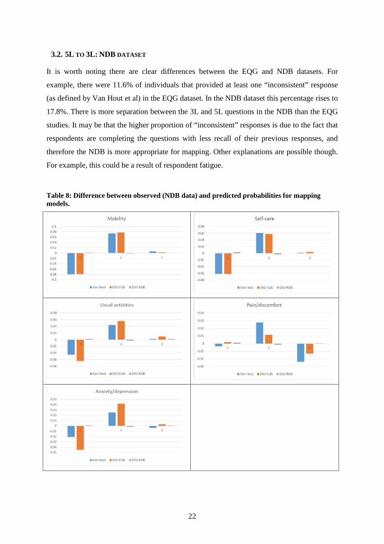
3.2. 5L TO 3L: NDB DATASET

It is worth noting there are clear differences between the EQG and NDB datasets. For

example, there were 11.6% of individuals that provided at least one “inconsistent” response

(as defined by Van Hout et al) in the EQG dataset. In the NDB dataset this percentage rises to

17.8%. There is more separation between the 3L and 5L questions in the NDB than the EQG

studies. It may be that the higher proportion of “inconsistent” responses is due to the fact that

respondents are completing the questions with less recall of their previous responses, and

therefore the NDB is more appropriate for mapping. Other explanations are possible though.

For example, this could be a result of respondent fatigue.

Table 8: Difference between observed (NDB data) and predicted probabilities for mapping models.

23

Table 8 shows the differences between the probabilities of being in each of the three response

categories and the observed data in the NDB, for the five health domains. It shows that the

DSU NDB model closely aligns to the observed data. Comparing the DSU EQG and van

Hout approaches, both of which were estimated using the EQG data, shows that the DSU

approach fits more closely for all response levels within the pain/discomfort domain. The van

Hout method fits more closely for all levels in the usual activities domain. Other domains are

mixed or very similar between the two approaches.

Table 9: Overall summary fit in the NDB dataset

ME MAE RMSE

van Hout 0.009 0.094 0.149

DSU EQG 0.020 0.100 0.148

DSU NDB 0.001 0.100 0.147

As with the EQG dataset, there are not large differences between any of the three measures

when considering summary fit statistics (Table 9). The DSU NDB method, for which these

figures represent a form of in-sample validation, has the best fit measured by ME and RMSE,

but the van Hout et al approach has a lower MAE.

A similar pattern is seen when considering the same measures by age and gender subgroups,

reported in Table 10. The DSU NDB method tends to perform better on measures of ME and

RMSE whilst the van Hout et al method does better on the MAE measures. It should again be

reiterated that these differences between the models are typically very small.

Figure 4 and Figure 5 show the closeness of fit for the DSU NDB model. In particular the

cumulative distribution plot shows very close in-sample fit.

24

Table 10: Ranking of fit compared to the NDB data by Mean Error, Mean Absolute Error and Root Mean Squared Error

Patient group N Percent ME MAE RMSE

van

Hout DSU EQG

DSU NDB

van Hout

DSU EQG

DSU NDB

van Hout

DSU EQG

DSU NDB

female <=25 25 0.48 2 1 3 1 2 3 1 2 3 female (25-35] 111 2.13 2 3 1 1 2 3 3 1 2 female (35-45] 252 4.84 1 3 2 1 2 3 1 2 3 female (45-55] 708 13.6 2 3 1 1 3 2 3 2 1 female (55-65] 1,300 24.98 2 3 1 1 3 2 3 2 1 female (65-75] 1,186 22.79 2 3 1 1 2 3 3 1 2 female >75 628 12.07 2 3 1 1 2 3 1 3 2 male <=25 1 0.02

male (25-35] 5 0.1 male (35-45] 19 0.37 male (45-55] 123 2.36 3 1 2 1 2 3 2 1 3

male (55-65] 303 5.82 2 3 1 1 3 2 2 3 1 male (65-75] 335 6.44 1 3 2 1 2 3 2 3 1 male >75 209 4.02 2 3 1 1 2 3 3 2 1

Total 5,205 100

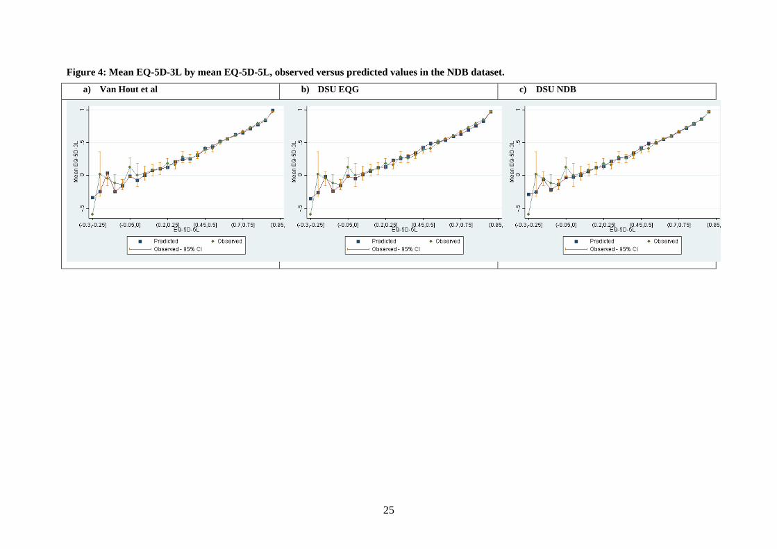
25

Figure 4: Mean EQ-5D-3L by mean EQ-5D-5L, observed versus predicted values in the NDB dataset. a) Van Hout et al b) DSU EQG c) DSU NDB

26

Figure 5: Observed versus predictive cumulative distribution function – NDB dataset a) Van Hout et al b) DSU EQG c) DSU NDB

27

3.3. ADDITIONAL COMPARISONS OF 5L TO 3L.

To further understand the drivers of the results, we calculated three new versions of the

crosswalk. First, we replicated the same methods as the van Hout et al “crosswalk” but used

the NDB dataset. Second, we created an amended version of the van Hout et al method but

instead of amending all the “inconsistent” responses, we use the original data (we refer to this

as the “unconstrained” method). We did this in both the EQG datasetii and the NDB dataset.

In total, this creates 6 different methods for mapping between 5L descriptive system data and

3L:

1) DSU copula model (estimated using EQG data)

2) DSU copula model (estimated using NDB data)

3) Crosswalk (EQG, unconstrained)

4) Crosswalk (EQG, constrained) – this is the van Hout et al method.

5) Crosswalk (NDB, unconstrained)

6) Crosswalk (NDB, constrained)

We calculated MAE and RMSE for all 6 methods, applied to both datasets. The rank

correlation coefficient between MAE and RMSE was 0.14, indicating very low correlation

between these two measures. This shows that MAE and RMSE are measuring different

things. They cannot be seen as measures of a single concept of “model fit”: there is no such

single concept.

We concentrate on the case which is more likely to replicate how the models will be used in

practice. We use the models estimated using the EQG as the reference dataset and compare

the out-of-sample predictions on the NDB dataset, which can be thought of as having

parallels with the use of mapping in a clinical study. The following rankings were observed

(where ≻ denotes the preferred model).

MAE: (4) ≻ (3) ≻ (1)

RMSE (1) ≻ (3) ≻ (4)

ii To abstract from differences arising from the small differences in samples between the models estimated using the EQG dataset due to missingness EQ-5D-3L and -5L individual dimensions, age and gender, we estimated all the models in the same sample as the DSU copula model (3,551). There are no significant differences in the transition probabilities between the original crosswalk model and the one estimated in the common sample.

28

Thus, MAE and RMSE rank the models in the complete reverse order. RMSE penalises large

errors more heavily and favours the DSU copula model whereas MAE favours the

constrained crosswalk.

We investigated the reasons why the performance of the van Hout et al model is very good in

terms of MAE, but less good in terms of RMSE. We identified a further issue when using

measures of fit based on errors in models where the underlying data has been amended as has

been done in the van Hout analysis. Probabilities equal to 1 (or 0) refer to a situation where

something is known with complete certainty. In such situations, there is no need for statistical

modelling. Setting a number of probabilities equal to 1 in the van Hout et al analysis implies

that any EQ-5D-5L health state description including any combination of levels equal to 1, 3

or 5 and identified as consistent will automatically have a zero error associated with it. These

zero errors artificially drive down measures of fit like MAE and RMSE. The effect of this is

greater the larger the proportion of these health states in the dataset.

In contrast, all statistical models which use sample probabilities will tend to look worse in

comparison unless the improvements in the errors for the rest of the observations are

sufficiently large to outweigh the inevitable increase in the error for the “consistent”

observations with health state descriptions combining the levels 1, 3, and 5.

To illustrate this further, consider respondents who give a 5L health state of 11111 (n=537 in

the EQG dataset). 500 (93.1%) of these in the EQG dataset also respond that they are in

11111 for the 3L health state. Using the van Hout et al approach, these individuals will have a

zero error associated with their response pairs. And the remaining 6.9% will have some error

associated with them. This large proportion of observations with zero errors will tend to drive

the MAE down but this will also cause the RMSE to rise, if imposing these restrictions

negatively affects the fit for other observations.

In contrast, any model based approach will try to replicate the full data. Thus, the 93.1% of

respondents will all have a small error associated with their observation pairs (it is not the

case that respondents at level 1 for the 5L will indicate with total certainty they are at level 1

for the 3L, as reported in Table 4). It is this which drives the performance of the approaches

in terms of summary fit and the apparent contradictory findings when using MAE compared

to RMSE.

29

There are 716 respondents in the EQG dataset that answer either 1, 3 or 5 on the 5L for each

dimension and provide 3L responses that van Hout et al define as “consistent” (that is, they

answer 1 if 5L = 1, 2 if 5L = 3 and 3 if 5L =5). MAE for these respondents using the van

Hout method is 0. The DSU EQG model has a MAE of 0.028. The DSU NDB model has a

MAE of 0.036. RMSE for the van Hout, DSU EQG and DSU NDB are 0, 0.037 and 0.050

respectively.

There are 84 respondents that answer either 1, 3 or 5 on the 5L for each dimension and

provide “inconsistent” responses for at least one dimension. MAE is 0.201, 0.175 and 0.168

for the van Hout, DSU EQG and DSU NDB models respectively. RMSE is 0.260, 0.232, and

0.222 for the same models. The ordering of the models is totally reversed compared to the fit

of the models in the “consistent” data.

There are 48 respondents that provide 5L responses at levels 2 or 4 for every dimension.

MAE for the same three models is 0.194, 0.184 and 0.178 respectively. RMSE is 0.260,

0.232 and 0.222 respectively.

This highlights that comparisons of summary measures of fit across the entire range of health

for mapping approaches mask differences between the methods. In particular, there are

differences in the methods between health states that are predominantly answered in a

manner that is defined as “consistent” in the van Hout approach, versus those that have a

greater number of “inconsistent” responses.

3.4. 3L TO 5L The two DSU copula based models are capable of estimating 5L utilities from 3L responses.

We present summaries of how the two models perform below. In the previous sections, there

was a common out of sample comparison that could be made between the van Hout et al

approach and the DSU EQG model. There is no common out-of-sample comparison that can

be made here as there are only two datasets.

Figure 6 and Figure 7 show the in-sample plots for the EQG and NDB copula based models.

For both models, there is very close alignment between observed and fitted data. There

appears to be a poorer fit, in both cases, around 0.4–0.5 on the 3L scale. However, the large

30

error bars indicate the paucity of data at these points. In the NDB, there is no error bar

because there is a single observation at this point.

Figure 6: DSU EQG in-sample

a) Mean 5L utility by mean 3L b) Cumulative distribution

Figure 7: DSU NDB in-sample

a) Mean 5L utility by mean 3L b) Cumulative distribution

Out-of-sample fit is demonstrated, for both models, in Figure 8 and Figure 9. These plots

again demonstrate good performance of both approaches, though as for any out-of-sample

examination, fit is not as good as in-sample. For the DSU EQG approach, there is some

evidence that mean predicted values are lower than mean observed values (in the NDB

dataset) for 3L scores around zero. For the DSU NDB approach, predicted 5L values based

on the EQG model are slightly higher than the observed means around 3L values of -0.1 and

0.2-0.3.

31

Figure 8: DSU EQG out-of-sample

a) Mean 5L utility by mean 3L b) Cumulative distribution

Figure 9: DSU NDB out-of-sample

a) Mean 5L utility by mean 3L b) Cumulative distribution

4. DISCUSSION AND RECOMMENDATIONS

For mapping from 3L to 5L, or for mapping from 5L utility values to 3L, there are two

currently available options: the DSU EQG or DSU NDB methods. Both of these methods

demonstrate very close in-sample fit when mapping from 3L to 5L. Furthermore, there are no

significant concerns identified from out-of-sample testing, and biases often seen in mapping

studies more generally are not present in the DSU approach (namely the tendency for simple

methods to overestimate utility for those in relatively poor health and underestimate it for

those in good health). There is little in the analyses we have performed to warrant a

preference for one approach over another. There are differences between the EQG and NDB

32

datasets concerning issues of study design (e.g. the degree of separation of questions, the

mode of administration, the language in which the questionnaires were conducted, and the

sampling methods). These differences mean that there is not an unambiguously preferred

dataset for mapping. However, the nature of the sampling frameworks, in particular the

inclusion of patients with a variety of medical conditions in the EQG data, may make this a

preferable selection for use in NICE appraisals at the current time.

We have also demonstrated that there is no single method to assess goodness of fit and

different measures favour different mapping approaches. When considering the relationship

between the discrete, descriptive system data and the different models, there are small

differences observed. In general, the DSU models perform slightly better than the van Hout et

al approach. We have shown how commonly used measures of fit for continuous data, MAE

and RMSE, give very different answers but are marginally better in general for the Van Hout

method. RMSE places a greater penalty on larger errors. More importantly, the method of

adjusting data that is deemed to be “inconsistent” in the van Hout et al approach, artificially

drives down these measures of fit overall and makes comparisons with methods that use the

real data questionable. Observations are adjusted in that some parts of an observation are

retained and other parts ignored. There are real differences between the mapping methods and

how they fit parts of the data, even though summary measures of fit across the spectrum of ill

health may only be marginally different.

All of the models we have compared are limited by the available data. We have concerns

about the appropriateness of both datasets for the purpose of mapping between 3L and 5L in a

UK context and across different diseases and technologies. It is not known whether the

ordering of 3L and 5L in a survey influences responses, or the extent of separation between

them to achieve independent responses. The NDB is restricted to a US/Canadian population

with rheumatic disease. The respondents are predominantly female (81%) and in much better

health than the respondents in the EQG data. Figure 5 shows that just 10.34% of the NDB

sample report 3L scores below 0.5.

Available information about the EQG study are much less detailed than the NDB approach,

in part because it was formed as a combination of add-ons to several separate studies in

different countries. There was relatively little separation between patients being asked the 3L

33

and the 5L, substantially less than the NDB, and this may result in patients providing

responses that are not biased by recall of their responses to the 3L.

Many may think that these datasets are relatively large at 3,691 and 5,299 respectively.

However, we consider them to be insufficient. In the EQG data only 119 of the possible 233

EQ-5D-3L utility values are observed. 29.30% of respondents report the same level in all

dimensions, 19.10%, 9.69% and 0.51% of respondents reported being in states 11111, 22222

and 33333 respectively. In the NDB only 83 of the 233 EQ-5D-3L utility values are observed

and 21.67% of respondents report the same level in all dimensions, 15.18%, 6.46% and

0.04% reported being in states 11111, 22222 and 33333 respectively. This could indicate that

responses are given without full consideration. We know that most of the 233 utility values

do appear in real patient records. For example, in the PROMS 2010-2014 data for knee

replacement procedures (n=320,000) we find 189 out of 233 possible utility values, and,

although econometric modelling is used to extrapolate to the areas where we do not have

data, better coverage in the data would provide greater confidence in the results.

Whatever future decisions are taken by NICE, and other decision making bodies, regarding

the 3L and 5L instruments, there will be a requirement to map between them for many years

to come. Given the potential impact, we consider it essential that a well-designed, large-scale

new data collection exercise be undertaken in order to estimate a definitive mapping that can

be used for decision making in the UK NHS.

5. CONCLUSIONS

NICE needs to recommend one approach for mapping in order to avoid complicating the

appraisal process and reduce opportunities for gaming.

If the 5L is recommended by NICE, mapping from 3L health states to 5L utility values

should be conducted using the DSU EQG based model. The current alternative is to use the

DSU NDB based model. Our recommendation is based solely on the belief that the EQG

dataset is more generalizable to the range of conditions NICE is likely to encounter.

Mapping from either 3L or 5L utility scores to their counterpart utility scores should also be

conducted using the DSU EQG based model, for the same reasons.

34

Standard measures of fit across the distribution of health do not reveal significant differences

in the performance of methods for mapping from 5L health states to 3L utility scores.

However, the manner in which data is deemed “inconsistent” and elements of it then ignored

in the van Hout et al approach does cause concern. The result of this approach is that it

generates zero errors for some parts of responses, and thus very good summary measures of

fit across the distribution, but it also results in larger errors in other areas. There are

differences in the results generated between the DSU approaches and the van Hout

approaches that are masked by summary measures of fit.

NICE may wish to recommend a consistent approach to mapping whether to 3L from 5L, or

vice versa, or from utility values rather than health state descriptions. It should be noted that

the DSU approach for mapping is a single model for all of these options, estimated jointly. In

this sense, it provides a completely consistent approach.

We also believe that all these mapping functions should be considered interim because of

limitations in the data. Given the importance of a single, robust approach to mapping, a

reference case dataset should urgently be commissioned with a detailed consideration of

study design to overcome deficiencies in existing data sources. That data collection needs to

consider the ordering of 3L and 5L, the degree of separation required, the sample size and

sampling frame, inter alia.

6. REFERENCES

1 NICE. Guide to the Methods of Technology Appraisal. 2013. 2 Herdman M, Gudex C, Lloyd A, et al Development and preliminary testing of the new five-level version of EQ-5D (EQ-5D-5L). Qual Life Res. 2011; 20(10): 1727–1736. 3 Devlin, N., Shah, K., Feng, Y., Mulhern, B., and van Hout, B. (2016). Valuing health related quality of life: An EQ-5D-5L value set for England. Technical Report 16.02, Health Economics & Decision Science, University of Sheffield. 4 Wailoo A, Hernandez Alava M, Grimm S, et al (2017) Comparing the EQ-5D-3L and 5L versions. What are the implications for cost effectiveness estimates? DSU report, available at http://www.nicedsu.org.uk/EQ5D5L(3038874).htm 5 Van Hout B, Janssen MF, Feng Y et al. (2012) Interim Scoring for the EQ-5D-5L: Mapping the EQ-5D-5L to EQ-5D-3L Value Sets, Value in Health, Vol. 15: 708-15. 6 Hernandez Alava M, Pudney S. Econometric modelling of multiple self-reports of health states: The switch from EQ-5D-3L to EQ-5D-5L in evaluating drug therapies for rheumatoid arthritis. Journal of health Economics, in press. Available at: http://www.sciencedirect.com/science/article/pii/S0167629616305070 (last accessed 7th July 2017)

35

7 Janssen, M.F., Pickard, A.S., Golicki, D. et al. Measurement properties of the EQ-5D-5L compared to the EQ-5D-3L across eight patient groups: a multi-country study Qual Life Res (2013) 22: 1717. doi:10.1007/s11136-012-0322-4 8 Wolfe, F. & Michaud, K. (2011), `The National Data Bank for rheumatic diseases: a multi-registry rheumatic disease data bank', Rheumatology 50, 16-24.