Methodology for service life prediction of external paint ... · Methodology for service life...

Methodology for service life prediction of external paint

finishes (on rendered facades)

Cristina de Vilhena Veludo Chai

Extended abstract

Supervisor: Doutor Jorge Manuel Caliço Lopes de Brito

Co-supervisor: Doutor Pedro Manuel dos Santos Lima Gaspar

May, 2011

1

1 Introduction

The main objective of this research is the development of a deterministic methodology for the service life

prediction of external paint finishes on rendered facades. This study is based on field survey data of in-

service conditions and the analysis is presented in the shape of degradation models through simple linear /

non-linear regression and multiple linear regression.

Service life prediction assumes a primary role as it allows a more rational use of construction elements. This

constitutes a useful tool in the definition of preventive maintenance plans providing an increase in

performance.

In spite of the very broad use of paint as an external finish on rendered facades, many studies have shown

that there is a great frequency of painting anomalies as this type of finish is very sensitive to degradation.

2 Framework of the proposed theme

The prediction of the service life of materials and construction components is a fairly recent concern,

especially in studies connected to the construction industry. The awareness of the importance of durability

only started to appear in developed countries in the sixties. The systematic approach of durability

measurement, in order to obtain data that would allow the prediction of service life, gained relevance only in

the eighties.

2.1 Service life concept

Service life is defined according to ISO 15686 as the period of time after construction during which

buildings and their materials equal or exceed the minimum performance requirements. Its definition involves

a prior definition of criteria of acceptance that varies in time, place, according to the measurer’s point of

view and, in fact, to all economic, political, aesthetic, environmental or normative contexts that frame

judgment on construction [Gaspar, 2009].

The end of service life represents the point in time, in which the material or component can no longer ensure

the activities they were developed for, by factors that are not always objective nor quantifiable. For

simplicity sake, it is usually considered that the end of a building’s service life occurs through functional

obsolescence, lack of economic viability or physical wear of its keys materials [Ang e Wyatt, 1999],

[Gaspar, 2001], [Gaspar e Brito, 2003c].

In this research, the chosen approach is based on the physical service life, in other words, the deterioration

due to the action of degradation agents and the natural aging of the element. Degradation can still be split

into aesthetical and functional categories, notably because in painted coatings the quality of the visual impact

shown by the material is also an important factor when determining the end of service life. The unfulfilled

criterion was deliberately left out of this work and instead degradation was regarded as a synergy of

pathological events that lead to the end of the element’s service life.

2.2 Maintenance and service life

According to Tekata et al. [2004], the necessity of maintenance is due both to the change of the building’s

conditions due to degradation - compromising the physical service life - and to the change of society’s

expectations and demands - compromising the functional service life.

The maintenance operations affect the behaviour of the elements in time changing the degradation models

(rise in performance) and the values of service lives enabling an optimization of their life cycle durations.

The role of maintenance is then crucial in order to intervene at the appropriate time avoiding the growth of

existing anomalies, saving precious resources and minimizing the costs involved [Flores e Brito, 2003c].

Extended abstract

Extended abstract

2

3 Problem definition

Paint continues to have a leading role as an external finish in both national and international construction

and, according to INE [2001], is the most used coating in Portugal.

Dependent on the design, application, drying process, environmental and exposure conditions, occasional

anomalies or irreversible degradation processes may emerge that disrupt not only the aesthetic and visual

quality of the facades but also compromise the protection coatings confer.

3.1 Anomalies characterization

The main anomalies affecting the paint were grouped in four categories:

Stains \ chromatic anomalies;

Cracking;

Adherence loss (peeling and blistering);

Cohesion loss (chalking).

According to experts, stains and chromatic alterations precede cracking, which may also precede blistering

and detachments, showing a growing hierarchy of seriousness between the three aforementioned groups.

3.2 Degradation factors specification

The concept of a degradation factor used in this study includes any factor that might influence the durability

of coatings, such as external (degradation agents) or internal (intrinsic characteristics of the material and its

interaction with the surface) factors. The purpose of taking them into account is to point out the different

behaviours and the interaction function with each other, working as filters that gather a set of buildings

according to their mutual characteristics.

The specification of the degradation factors accounted for in this study relies on the adopted methodology

being able to identify, estimate, quantify and specify; therefore the study focuses on the importance of the

following factors, connected to the durability of paint:

Exposure to humidity;

Distance from the ocean;

Wind/rain action;

Distance from pollution sources;

Facade orientation;

Type of paint;

Colour of the coating;

Pellicle texture;

Surface preparation.

4 Field data

The field work was performed on Lisbon’s building stock, on facades exposed to several degradation agents,

regardless of their construction typology. Within this framework, 160 subjects were analysed, corresponding

to 220 coatings.

The visual data resulting from the survey of the facades were registered on an inspection sheet created in

order to systematically organize the recorded information. It contains the field variables needed to define, on

a global scale, the facade degradation and the analysis of the degradation related to each considered factor,

thus forming a database of in-service paint finishes. Each analysed facade has its own inspection sheet,

where the input of the service life prediction method further developed is listed.

Extended abstract

3

4.1 Definition of levels of degradation

According to several authors, field work results can provide a distorted image of reality by not taking into

account some important aspects, e.g. the seriousness and intensity of the registered anomalies. In order to

overcome this, levels or thresholds of degradation were defined for the registered defects according to their

severity and the group of anomalies to which they belong.

Several authors developed scales of degradation, in order to build models of service life prediction of the

building elements. Gaspar and Brito [2005], Bordalo [2008] and Silva [2009] determine the anomaly

seriousness according to the anomaly type and affected area, by setting five levels of degradation (where 0

means no visible degradation and 4 indicates general degradation); Shohet and Paciuk [2004] established a

physical and visual scale concerning external claddings that takes into account the affected area and the

dimension of the anomalies, ranging from 0 to 100 (100 represents a flawless coating or with no signs of

problems). Lastly, Gaspar [2009] creates a degradation atlas, which consists of a written and photographic

information list referring to the several types of anomalies that affect renders, ranked according to their

degradation level.

In the current analysis, the criterion used to define the degradation levels was seriousness, connected to the

consequences, either in the protection given or in the visual perception. The range or area affected is a

different concept, since it is another aspect that should be considered when assessing the global degradation

level and therefore it is a very important definition in the field work.

Visual and physical scales to evaluate the detected degradation anomalies were created, based on the existing

quantification norms ([NP EN ISO 4628-1:2005], [NP EN ISO 4628-2:2005], [NP EN ISO 4628-4:2005],

[NP EN ISO 4628-5:2005], [NP EN ISO 4628-7:2005]). For each group of anomalies, a 0-4 degradation

scale was set, where 0 represents no visible degradation and level 4 represents generalized degradation; the

criteria adopted were the following:

Quantity or density, for cracking (Table 1);

Quantity, for chalking (Table 2);

Hierarchy of the anomalies according to the severity and intensity of the alteration, for stains/colour

changes (Table 3);

Hierarchy of the anomalies according to the severity, density and dimension, for loss of adherence

(Table 4).

Table 1 - Definition of degradation levels for cracking

Degradation level Level 0 Level 1

Good condition

Level 2

Slight degradation

Level 3

Moderate

degradation

Level 4

Generalized

degradation

Quantity No visible

degradation

Small number of

cracks

Moderate number

of cracks

Considerable

number of cracks High number of cracks

Visual scale [NP

EN ISSO 4628-4,

2005

Table 2 - Definition of degradation levels for chalking

Degradation level Quantity

Level 0 No degradation visible

Level 1 - Good Clearly perceptible

Level 3 - Moderate wear-and-tear Quite perceptible

Level 4 - Generalized degradation Very perceptible

Extended abstract

4

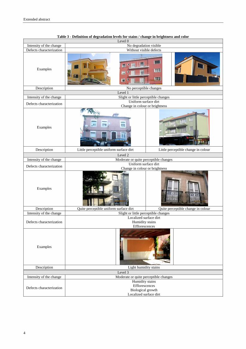
Table 3 - Definition of degradation levels for stains / change in brightness and color

Level 0

Intensity of the change No degradation visible

Defects characterization Without visible defects

Examples

Description No perceptible changes

Level 1

Intensity of the change Slight or little perceptible changes

Defects characterization Uniform surface dirt

Change in colour or brightness

Examples

Description Little perceptible uniform surface dirt Little perceptible change in colour

Level 2

Intensity of the change Moderate or quite perceptible changes



Examples

Description Quite perceptible uniform surface dirt Quite perceptible change in colour

Intensity of the change Slight or little perceptible changes

Defects characterization

Localized surface dirt

Humidity stains

Efflorescences

Examples

Description Light humidity stains Level 3

Intensity of the change Moderate or quite perceptible changes

Defects characterization

Humidity stains

Efflorescences

Biological growth

Localized surface dirt

Extended abstract

5

Examples

Description Quite perceptible humidity stains Quite perceptible biological growth

Examples

Description Quite perceptible localized surface dirt Quite perceptible

efflorescences

Intensity of the change High or very perceptible changes



Examples

Description

Very perceptible uniform

surface dirt and change in

colour

Very perceptible Localized surface

dirt

Very perceptible change in

colour (discoloration)

Level 4

Intensity of the change High or very perceptible changes

Defects characterization Biological growth

Examples

Description Very perceptible biological growth

4.2 Characterization of the sample studied

Based on survey information and having set the classification criteria of the different variables, it is possible

to characterize the samples (160 buildings and 220 facades) in the following way:

The majority are housing units (67%), from which 81% have a compact structure and 43% low

height;

20% are less than 1 km from the sea, 32% between 1 and 5 km and 48% more than 5 km;

47% have recurring exposure to humidity while 53% have negligible exposure;

22% are slightly exposed to wind/rain, 45% moderately exposed and 33% severely exposed;

The parameter that shows the greatest heterogeneity is “distance from pollution sources”; only 21%

lack exposure;

The average age of the last painting is 6 years; 29% are less than 4 year olds, 27% between 4 and 8

years, 29% between 8 and 12 years and 16% more than 12 years;

The distribution of the facades regarding their orientation is fairly regular for all quadrants;

Extended abstract

6

40% are plain paint, 38% are elastic membranes and 22% are textured paint;

Within the 40% plain paints, 63% are traditional plain paint, 27% are non-traditional plain paint and

10% are paints made with silicates and silicone;

The majority of the buildings (50%) have colours between yellow, orange and light pink and 27%

are white; dark colours have little relevance;

56% of the buildings have smooth finishing and 44% have rough finishing.

Table 4 - Definition of degradation levels for peeling and blistering

Level 0

Defect characterization No degradation visible

Level 2

Defect characterization Blistering

Quantity and size Small amount and size up to 3 cm

Visual scale [NP EN ISO 4628-2,

2005 e NP EN ISO 4628-5, 2005]

Level 3


Quantity and size Small amount and size between 3 - 5 cm Moderate amount and smaller than 3 cm


2005 e NP EN ISO 4628-5, 2005]

Defect characterization Peeling

Quantity and size Small amount (area affected up to 1%) e size up to 3 cm


2005 e NP EN ISO 4628-5, 2005]

Level 4


Quantity and size Larger than 5 cm,

regardless of the amount

Dense pattern regardless of

the size

Moderate amount e and

dimension between 3 - 5 cm


2005 e NP EN ISO 4628-5, 2005]

Defect characterization Peeling

Quantity and size Dense and moderate pattern (affected area

higher than 1%) regardless of the size Small amount and larger than 5 cm


2005 e NP EN ISO 4628-5, 2005]

5 Data analysis

The analysis methodology can be divided in four different steps: definition of the minimum level of

acceptance in paint finishes, quantification of degradation as one parameter that can translate the global level

Extended abstract

7

of facade degradation, definition of the relationship between this parameter and the condition, application of

the graphical method (degradation models) and identification of a reference service life.

Conceptually, it is considered that degradation means loss of performance, and thus its progression provides

an understanding of the loss of performance during the service life of coatings.

5.1 Minimum performance level

In this study, the definition of the minimum performance level follows the same criterion as Gaspar [2002],

Bordalo [2008] and Silva [2009], considering that the minimum performance level is equal to level 3

(moderate degradation). After this limit, it is considered that the coatings reach the end of their life cycle and

are not fit to perform the function for which they were designed, leading to a generalized repair in order to

re-establish the characteristics essential to its proper performance.

The advantage of this method is to be able to adopt different criteria for coating acceptance, according to

several profile analysis. In each situation, the decision maker should identify criteria to focus on, adjust the

threshold level of their demand - which may be higher or lower than that considered - and obtain the

remaining lifetime for the case study.

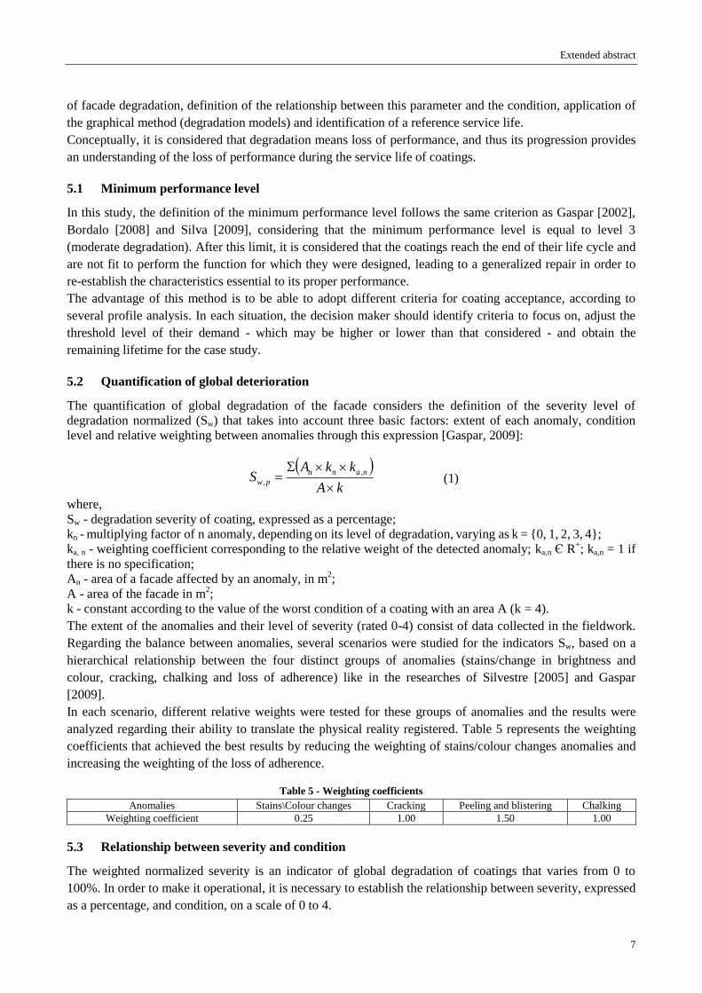
5.2 Quantification of global deterioration

The quantification of global degradation of the facade considers the definition of the severity level of

degradation normalized (Sw) that takes into account three basic factors: extent of each anomaly, condition

level and relative weighting between anomalies through this expression [Gaspar, 2009]:

(1)

where, Sw - degradation severity of coating, expressed as a percentage;

kn - multiplying factor of n anomaly, depending on its level of degradation, varying as k = {0, 1, 2, 3, 4};

ka, n - weighting coefficient corresponding to the relative weight of the detected anomaly; ka,n Є R+; ka,n = 1 if

there is no specification;

An - area of a facade affected by an anomaly, in m2;

A - area of the facade in m2;

k - constant according to the value of the worst condition of a coating with an area A (k = 4).

The extent of the anomalies and their level of severity (rated 0-4) consist of data collected in the fieldwork.

Regarding the balance between anomalies, several scenarios were studied for the indicators Sw, based on a

hierarchical relationship between the four distinct groups of anomalies (stains/change in brightness and

colour, cracking, chalking and loss of adherence) like in the researches of Silvestre [2005] and Gaspar

[2009].

In each scenario, different relative weights were tested for these groups of anomalies and the results were

analyzed regarding their ability to translate the physical reality registered. Table 5 represents the weighting

coefficients that achieved the best results by reducing the weighting of stains/colour changes anomalies and

increasing the weighting of the loss of adherence.

Table 5 - Weighting coefficients

Anomalies Stains\Colour changes Cracking Peeling and blistering Chalking

Weighting coefficient 0.25 1.00 1.50 1.00

5.3 Relationship between severity and condition

The weighted normalized severity is an indicator of global degradation of coatings that varies from 0 to

100%. In order to make it operational, it is necessary to establish the relationship between severity, expressed

as a percentage, and condition, on a scale of 0 to 4.

kA

kkAS nann

pw

,

,

Extended abstract

8

The ratio between level of degradation and severity, expressed in level of condition, was based on the model

of Gaspar [2009], already adopted by Silva [2009]. There is a consistency between the observed degradation

in the case studies and degradation level assigned to them by the severity of their value. The correspondence

table adopted is presented in Table 6.

Table 6 - Correspondence between the degradations indicators

Severity Degradation levels

Sw,p ≤ 1% 0

1% < Sw,p ≤ 10% 1

10% < Sw,p ≤ 20% 2

20% < Sw,p ≤ 40% 3

Sw,p 40% 4

After defining the relationship between severity and condition, it is possible to divide the sample into five

intervals, depending on the values obtained for the weighted normalized severity (Figure 1) and thus analyze

the distribution of case studies according to this indicator and overall levels of degradation (Figure 2).

Figure 1 - Distribution of degradation in 220 case studies in the five different degradation levels 0, 1, 2, 3 and 4

Figure 2 - Sample distribution according to severity and degradation levels

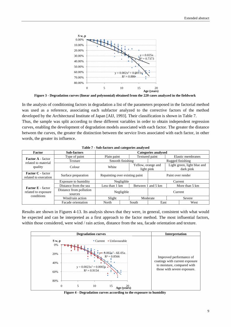
5.4 Degradation models through simple linear / non-linear regression

After the degradation severity was defined and the age of the coating for each case study was known, it was

possible to build a graph containing the overall sample. Using statistical techniques, linear and polynomial

decay curves were adjusted to the points, representing the performance loss of the paintings over time

(Figure 3).

The configuration obtained for the polynomial curve shows a convex development, expressing a trend of

paint coatings to slowly decay, but whose effects are felt cumulatively. As shown in Figure 3, up to five

years, the rate of deterioration is low, followed by an accelerating trend of the degradation potential.

0%

20%

40%

60%

80%

0 5 10 15 20

Sw, p

Age (years)

17%

36%

23%15%

9%

0%

20%

40%

60%

80%

Less than

1%

Beween 1

and 8%

Between

8 and

20%

Beween

20 and

45%

More

than 45%

17%

36%23%

15%

9%Level 0

Level 1

Level 2

Level 3

Level 4

1%

10%

20%

40%

Extended abstract

9

Figure 3 - Degradation curves (linear and polynomial) obtained from the 220 cases analyzed in the fieldwork

In the analysis of conditioning factors in degradation a list of the parameters proposed in the factorial method

was used as a reference, associating each subfactor analyzed to the corrective factors of the method

developed by the Architectural Institute of Japan [AIJ, 1993]. Their classification is shown in Table 7.

Thus, the sample was split according to these different variables in order to obtain independent regression

curves, enabling the development of degradation models associated with each factor. The greater the distance

between the curves, the greater the distinction between the service lives associated with each factor, in other

words, the greater its influence.

Table 7 - Sub-factors and categories analysed

Factor Sub-factors Categories analysed

Factor A - factor

related to material

quality

Type of paint Plain paint Textured paint Elastic membranes

Texture Smooth finishing Rugged finishing

Colour White Yellow, orange and

light pink

Light green, light blue and

dark pink

Factor C - factor

related to execution Surface preparation Repainting over existing paint Paint over render

Factor E - factor

related to exposure

conditions

Exposure to humidity Negligible Current

Distance from the sea Less than 1 km Between 1 and 5 km More than 5 km

Distance from pollution

sources Negligible Current

Wind/rain action Slight Moderate Severe

Facade orientation North South East West

Results are shown in Figures 4-13. Its analysis shows that they were, in general, consistent with what would

be expected and can be interpreted as a first approach to the factor method. The most influential factors,

within those considered, were wind / rain action, distance from the sea, facade orientation and texture.

Degradation curves Interpretation

Improved performance of

coatings with current exposure

to moisture, compared with

those with severe exposure.

Figure 4 - Degradation curves according to the exposure to humidity

y = 0.002x2 + 0.0011x

R² = 0.886

y = 0.025x

R² = 0.7373

0.00%

10.00%

20.00%

30.00%

40.00%

50.00%

60.00%

70.00%

80.00%

0 5 10 15 20

S w, p

Age (years)

y = 0.002x2 - 6E-05x

R² = 0.8566

y = 0.0023x2 + 0.0003x

R² = 0.9154

0%

20%

40%

60%

80%

0 5 10 15 20

S w, p

Age (years)

Current Unfavourable

Extended abstract

10


Improved performance of the

coatings more than 5 km from

the sea, followed by those

between 1 and 5 km, and

finally those less than 1 km.

Figure 5 - Degradation curves according to the distance from the sea


Inconclusive ( results

inconsistent with those

expected)

Figure 6 - Degradation curves according to the distance from pollution sources


Improved performance of the

facades slightly exposed to

wind/rain action, followed by

those moderately exposed, and

finally those severely exposed

Figure 7 - Degradation curves according to wind / rain action



facades facing North and East

Faster degradation in the

facades facing South and West

Figure 8 - Degradation curves according to the orientation of the facade

y = 0.0022x2 + 0.0014x

R² = 0.9355

y = 0.0022x2 + 0.0007x

R² = 0.8823

y = 0.002x2 - 7E-07x

R² = 0.8622

0%

20%

40%

60%

80%

0 5 10 15 20

S w, p

Age (years)

Less than 1 km Between 1 and 5 km

More than 5 km

y = 0.0019x2 + 0.0013x

R² = 0.9116

y = 0.0021x2 + 0.0002x

R² = 0.87

0%

20%

40%

60%

80%

0 5 10 15 20

S w, p

Age (years)

Unfavourable Current

y = 0.0019x2 + 0.0008x

R² = 0.7998

y = 0.0023x2 - 0.0011x

R² = 0.9384

y = 0.0028x2 - 0.0049x

R² = 0.8607

0%

20%

40%

60%

80%

0 5 10 15 20

S w, p

Age (years)

Slight Moderate Severe

y = 0.0015x2 + 0.0044x

R² = 0.7554

y = 0.002x2 - 0.0002x

R² = 0.8623

y = 0.0022x2 + 0.0002x

R² = 0.9409

y = 0.0019x2 + 0.0049x

R² = 0.9355

0%

20%

40%

60%

80%

0 5 10 15 20

S w, p

Age (years)

North East West South

Extended abstract

11


Short term: inconclusive

(overlapping curves) Long term: improved

performance of textured paints,

followed by membranes and,

finally, smooth paints

Figure 9 - Degradation curves according to the type of paint


Inconclusive (overlapping

curves)

Figure 10 - Degradation curves according to the colour of the paint



coatings with rough finish

Figure 11 - Degradation curves according to the finishing of the paint



facades located more than 1 km

from the river compared with

those located within 1 km

Figure 12 - Degradation curves according to the distance from the river (buildings located in Lisbon)

y = 0.0018x2 + 0.0024x

R² = 0.8121

y = 0.0023x2 + 0.0001x

R² = 0.907

y = 0.0001x3 + 0.0004x2 + 0.006x

R² = 0.9428

0%

20%

40%

60%

80%

0 5 10 15 20

S w, p

Age (years)

Textured paint Elastic membranes Plain paint

y = 0.0021x2 + 1E-04x

R² = 0.8931

y = 0.0019x2 + 0.0023x

R² = 0.8904

y = 0.0025x2 - 0.0044x

R² = 0.9109

0%

20%

40%

60%

80%

0 5 10 15 20

S w, p

Age (years)

Absorption coefficient 0,2 - 0,3Asorption coefficient 0,3 - 0,5Absorption coefficient 0,5 - 0,7

y = 0.0019x2 + 0.0018x

R² = 0.8691

y = 0.0025x2 - 0.0024x

R² = 0.9205

0%

20%

40%

60%

80%

0 5 10 15 20

S w,p

Age (years)

Rugged finishing Smooth finishing

y = 0.0021x2 - 0.0013x

R² = 0.8724

y = 0.0023x2 - 0.0019x

R² = 0.8193

0%

20%

40%

60%

80%

0 5 10 15 20

S w, p

Age (years)

More than 1 km Less than 1 km

Extended abstract

12



paints applied directly on

render (results with little

statistical validity due to the

small number of cases - 46

facades)

Figure 13 - Degradation curves according to the surface preparation (46 paints)

5.5 Degradation models through multiple linear regression

The degradation is defined by a number of factors that together contribute to the deterioration of paint

finishes thus ending their service life. This sub-chapter focuses on analyzing the simultaneous effect of the

considered parameters, allowing ranking their influence on degradation. This can be accomplished through a

regression analysis where the relationship, called the regression function, between one variable y, called the

dependent variable, and several others xi, called the independent variables, is studied.

The degradation model through multiple linear regression is given by the equation (2):

y = b0 + b1.x1 + b2.x2 + ... + bp.xp + Ɛ = b0 + i

p

i

i xb1

+ Ɛ (2)

where: y - dependent variable predicted by a regression model; p - number of independent variables (number

of coefficients); xi - independent variable (i=1, 2, …. p); b0 - constant; bi - coefficient corresponding to

independent variable xi (i=1, 2, …. p); Ɛ - random errors of the model.

In the performed analysis, software SPSS (Statistical Package for Social Sciences) was used and the

Stepwise method was chosen. In this method, the independent variables that are not significant, i.e.

representative of the dependent variable, are excluded. Moreover, the effects of multicollinearity are

eliminated [Silva et al., 2011, citing Leung et al., 2001].

When developing the model, the qualitative ranks of each degradation factor were replaced by figures, using

numerical values. These were calculated as the ratio between the predicted service life (found through the

interception between the horizontal line at Sw = 20% and the corresponding degradation curve) and the

reference service life (9.75 years). The model that allows the best results takes into account three different

independent variables: age, distance from the sea and orientation of the facade, while b0 ≠ 0.

The significance of the model is analyzed in two different ways: the first consists on a significance test of all

the coefficients in the regression model while the second considers the significance of the individual

coefficients, both performed through hypothesis tests (Table 8).

Table 8 - Hypothesis tests reflecting regression model significance

Null hypothesis (H0): Alternative hypothesis (H1):

Significance test of all coefficients in the

regression model H0: b0 = b1 = … = 0

H1: є i: bi ≠ 0 (i.e. there is at least one

coefficient different than zero).

Significance test of the individual coefficients H0: bi = 0 H1: bi ≠ 0

The probability that the null hypothesis is rejected when true is designated by the term α, and the level of

significance; (1- α) represents the level of reliability. In this work a significance level of 10% is used which

corresponds to a standard value.

The significance of the sum of all the coefficients in the regression model can be analyzed through the results

in the Anova table (part 1) in Table 9. In fact, through these results the null hypothesis can be tested by the

y = 0.0019x2 + 0.0018x

R² = 0.8493

y = 0.0023x2 - 0.0024x

R² = 0.7033

0%

20%

40%

60%

80%

0 5 10 15 20

S w, p

Age (years)

Paint over render Repainting over existing paint

Extended abstract

13

so called F test, which represents the ratio between the variance explained by the model and the variance not

explained by the model (Snedecor’s distribution).

Table 9 - Table Anova (Part 1): Significance test of all coefficients in the regression model

gl SQ MQ F Significance F (p)

Regression 3 5.321106633 1.773702211 354.300939 4.10632-83

Residual (error) 216 1.081339718 0.005006202

Total 219 6.402446351

The probability p = P (F > Fmodel) defines the probability of the lowest level of significance leading to

rejection of H0. Since p = 4.10632× 10-83

< α = 0.10, H0 is rejected at a level of 10%, i.e. at least one of the

coefficients bi and the corresponding variable xi in the regression model are significant.

The significance of the individual coefficients xi included in a multiple linear regression model with p

independent variables can be tested by performing a significance test on the parameter bi/ S(bi) with a

Student’s t-test. Like in the F test, here the value of p is compared to the significance level α, for each of the

coefficients. Table 10 presents the obtained results.

Table 10 - Table Anova (Part 2): Significance test of the individual coefficients

Variables Coefficients (bi) Standard error (S(bi)) t Stat p value

Constant (b0) 0.4734 0.1715 2.7602 0.0063

Age (x1) 0.0353 0.0011 31.1710 6.802-82

Distance from the sea (x2) -0.2618 0.1438 -1.8207 0.0700

Orientation of the facade (x3) -0.3175 0.0906 -3.5028 0.0006

Table 10 shows that for all variables, p < α = 0.10 and therefore they are all representative of the severity.

Once the significance of the sum of all the coefficients and the significance of the individual coefficient are

verified, the regression statistics output can be analyzed (Table 11).

Table 11 - Regression statistics output

Multiple R (R) 0.9116

R Square (R2) 0.8311

Adjusted R Square (R2ajusted) 0.8288

Standard error (σ) 0.0708

Observations (n) 220

This analysis reveals a strong correlation (R = 0.91) within the set of coefficients and that 83% of the

variability of the severity is explained by age, solar orientation and distance from the sea (R2adjusted = 0.83)

while the remaining 17% is due to external factors, not considered in this study.

However, the model relies in the validity of some assumptions which have to be verified (residuals analysis

and analysis of existence of multicollinearity). After verifying that the residuals (ej) follow a Normal

distribution (ej ~ N(0, σ2)), E(ej) = 0, Var(ej) = σ

2, and that the independent variables do not exhibit a linear

correlation, it is concluded that the severity of the degradation can be explained through the three

independent variables: age, distance from the sea and solar orientation, using the following equation (3):

Severity = 0.4734 + 0.0353 Age - 0.2618 Distance from the sea - 0.3175 Solar orientation (3)

6 Discussion of results

After the minimum performance level of 20% has been established, the reference service life (RSL) is

defined by the two following degradation models:

Extended abstract

14

The degradation model through simple non-linear regression, where the RSL is obtained graphically by

intercepting the degradation curve and the horizontal line corresponding to the minimum level of

performance;

The degradation model through multiple linear regression, where the average RSL is obtained

numerically by solving the equation of the regression curve x1 (age) for y = 0.20.

Results are shown in Table 12 as well as the values of service lives defined in other studies.

Table 12 - Service life values according to the present investigation and others studies

Paint finish

Source Reference service life (years)

Current

analysis

Degradation model through simple non-linear regression 9.7

Degradation model through multiple linear regression (average) 8.5

Flores-Colen [2002] 5

Japanese Guide [AIJ, 1993] More than 10

Guarantee of paint products (average) 5

Decree No. 24/2011 8

Cementitious renders

Source Reference service life (years)

Gaspar [2009] 21

The results are well within the expected range, according to research in this area and addressing the

perception among technicians about what durability of paintings concerns. These results can be interpreted as

a sign of the ability of the proposed methodology to describe the degradation.

The adopted methods proved to be a precise system within the prediction of service live of facade paintings,

allowing the identification of the main variables for the development of prediction methodologies: average

curves of degradation and reference service lives. This method has the advantage of allowing more

information to be added over time, and therefore, as knowledge develops, it is suggested that more factors of

degradation ought to be considered and the results transposed to the factorial method.

References

AIJ - Architectural Institute of Japan (1993), The English Edition of Principal Guide for Service Life

Planning of Buildings, commented edition, AIJ, Tokyo, Japan, 98 p.

Silva A., Brito J. de, Gaspar P. (2011), Service life prediction model applied to natural stone wall claddings

(directly adhered to the support), Construction and Building Materials, In Press

Ang, G.K.I.; Wyatt, D.P. (1999), Performance concept in procurement of durability and serviceability of

buildings, 8th International Conference on Durability of Buildings Materials and Component, Vancouver,

Canada, pp. 1821-1832.

Bordalo, R. (2008), Previsão da vida útil dos revestimentos cerâmicos aderentes em fachada, Dissertação de

Mestrado Integrado em Engenharia Civil, Instituto Superior Técnico, Universidade Técnica de Lisboa,

Lisboa, Portugal, 130 p.

Flores, I. (2002), Estratégias de manutenção. Elementos da envolvente de edifícios correntes, Dissertação de

Mestrado em Construção, Instituto Superior Técnico, Universidade Técnica de Lisboa, Lisboa, 180 p.

Flores, I.; Brito, J. de (2003c), A influência de alguns parâmetros na fiabilidade de estratégias de

manutenção, 3º Encore - Encontro sobre Conservação e Reabilitação de edifícios, LNEC, Lisboa, Portugal,

pp. 1017-1026

Gaspar, P. (2001), O layering como estratégia para o aumento da vida útil funcional das construções,

Construção 2001, Instituto Superior Técnico, Lisboa, Portugal, pp. 945-952.

Gaspar, P. (2009), Vida útil das construções: desenvolvimento de uma metodologia para a estimativa da

durabilidade de elementos da construção. Aplicação a rebocos de edifícios correntes, Tese de Doutoramento

em Ciências da Engenharia, Instituto Superior Técnico, Universidade Técnica de Lisboa, Lisboa, Portugal,

330 p.

Extended abstract

15

Gaspar, P; Brito, J. de (2003), O ciclo de vida das construções - critérios de análise, Arquitectura e Vida,

42, pp. 98-103.

Gaspar, Pedro; Brito, J. de (2005b), Assessment of the overall degradation level of an element, based on a

field data, 10th International Conference on Durability of Buildings Materials and Components (DBMC),

Lyon, France, pp. 1043-1050.

INE - Instituto Nacional de Estatística (2001), Estatísticas nacionais - Censos 2001.

Leung Arthur W. T., Tam C. M., Liu D. K. (2001), Comparative study of artificial neural networks and

multiple regression analysis for predicting hoisting times of tower cranes, Building and Environment 36(4),

pp. 457-467.

NP EN ISO 4628-1 (2005), Tintas e vernizes. Avaliação da degradação de revestimentos. Designação da

quantidade e dimensão de defeitos e da intensidade das alterações uniformes de aspecto. Parte 1:

Introdução geral e sistema de designação, Instituto Português das Qualidade, Lisboa, Portugal, 8 p.


quantidade e dimensão de defeitos e da intensidade das alterações uniformes de aspecto. Parte 2: Avaliação

do grau de empolamento, Instituto Português das Qualidade, Lisboa, Portugal, 16 p.



do grau de fissuração, Instituto Português das Qualidade, Lisboa, Portugal, 20 p.

NP EN ISO 4628-5 (2005) Tintas e vernizes. Avaliação da degradação de revestimentos. Designação da


do grau de descamação, Instituto Português das Qualidade, Lisboa, Portugal, 11 p.

NP EN ISO 4628-7 8 (2005), Tintas e vernizes. Avaliação da degradação de revestimentos. Designação da

quantidade e dimensão de defeitos e da intensidade das alterações uniformes de

aspecto. Parte 7: Avaliação do grau de pulverulência pelo método do tecido aveludado, Instituto Português

das Qualidade, Lisboa, Portugal, 8 p.

Shohet, I.; Paciuk, M. (2004), Service life prediction of exterior cladding components under standard

conditions, Construction Management and Economics, 22(10), pp. 1081-1090.

Silva, A. (2009), Previsão da vida útil de revestimentos de pedra natural de paredes, Dissertação de

Mestrado Integrado em Engenharia Civil, Instituto Superior Técnico, Universidade Técnica de Lisboa,

Lisboa, Portugal, 140 p.

Silva A., Brito J. de, Gaspar P. (2011), Application of a factor method to stone cladding using advanced

statistical tools, Automation in Construction, submetido para publicação.

Silvestre, J. (2005), Sistema de Apoio à Inspecção e Diagnóstico de Anomalias em Revestimentos Cerâmicos

Aderentes, Dissertação de Mestrado em Construção, Instituto Superior Técnico, Universidade Técnica de

Lisboa, Lisboa, Portugal, 172 p.

Takata, S.; Kimura, F.; Van Houten, F.; Westkämper, E.; Shpitalni, M; Ceglarek, D; Lee, Jay (2004),

Maintenance: Changing role in life cycle management, CIRP annals, 53(2), pp. 643-655.

Methodology for service life prediction of external paint ... · Methodology for service life...

Documents

Transcript of Methodology for service life prediction of external paint ... · Methodology for service life...