Methodology for Avoided Degradation through Fire Management

VCS Methodology

VM0029

Methodology for Avoided Forest Degradation through Fire Management

Version 1.0

8 May 2015

Sectoral Scope 14

VM0029, Version 1.0

Sectoral Scope 14

Methodology developed by:

Mpingo Conservation and Development Initiative (MCDI), Tanzania

In partnership with:

University of Edinburgh

University College London

Value for Nature Consulting

Methodology funded by:

The Royal Norwegian Embassy, Tanzania

VM0029, Version 1.0

Sectoral Scope 14

Table of Contents

1 Sources ......................................................................................................................... 4

2 Summary Description of the Methodology ...................................................................... 4

3 Definitions ...................................................................................................................... 6

4 Applicability Conditions .................................................................................................. 8

5 Project Boundary ........................................................................................................... 9

5.1 Spatial extent .................................................................................................... 9

5.2 Upper and lower carbon density boundaries of the project areas ...................... 9

5.3 Delineation of project boundaries ...................................................................... 9

5.4 Greenhouse gases and carbon pools ............................................................. 10

6 Baseline Scenario ........................................................................................................ 12

7 Additionality ................................................................................................................. 14

8 Quantification of GHG Emission Reductions and Removals ........................................ 14

8.1 Baseline Emissions ......................................................................................... 14

8.2 Project Emissions ........................................................................................... 24

8.3 Leakage .......................................................................................................... 29

8.4 Net GHG Emission Reductions and Removals ............................................... 32

9 Monitoring .................................................................................................................... 33

9.1 Data and Parameters Available at Validation .................................................. 33

9.2 Data and Parameters Monitored ..................................................................... 43

9.3 Description of the Monitoring Plan .................................................................. 50

10 References .................................................................................................................. 56

Appendix 1: GapFire Description......................................................................................... 58

Appendix 2: The Rothermel Model ...................................................................................... 81

VM0029, Version 1.0

Sectoral Scope 14

1 SOURCES

This methodology uses the latest versions of the following tools and modules:

VT0001 Tool for the Demonstration and Assessment of Additionality in VCS AFOLU

Project Activities

VMD0013 Estimation of greenhouse gas emissions from biomass and peat burning

(E–BPB)

2 SUMMARY DESCRIPTION OF THE METHODOLOGY

Additionality and Crediting Method

Additionality Project Method

Crediting Baseline Project Method

This methodology applies to projects that implement preventative early burning activities in

miombo woodlands in the Eastern Miombo ecoregion of Africa. As specified by the World

Wildlife Fund1, the Eastern Miombo ecoregion consists of a relatively unbroken area covering

the interior regions of southeastern Tanzania and the northern half of Mozambique, with a few

patches extending into southeastern Malawi. The Central Zambezian Miombo Woodland

ecoregion lies beyond Lake Malawi to the west, while north, the ecoregion is bordered by

Acacia-Commiphora Bushland and Thicket belonging to the Somali-Masai phytochorion

(White 1983). The East African coastal mosaic of White’s (1983) Zanzibar-Inhambane

Regional Center of Endemism lines the shore. The Zambezian and Mopane Woodland

ecoregion lies to the south.

This ecoregion is separated from other miombo ecoregions in that it is mostly confined to

lower elevations of the East African Plateau, and is dominated by the floristically

impoverished ‘drier Zambezian miombo woodland’ outlined by White (1983). Dominant tree

species include Brachystegia spiciformis, B. boehmii, B. allenii, and Julbernardia globiflora. In

areas of higher rainfall, a transition to wetter miombo occurs (White 1983). This ecoregion is

separated from adjacent ecoregions to the west by Lake Malawi and the Shire River, running

south from Mount Mulanje. In the north it is separated from the Central Zambezian Miombo

Woodland ecoregion by the Eastern Arc and Southern Rift Montane areas.

Several rivers traverse the Eastern Miombo ecoregion in a predominantly west-east direction;

these include the Rufiji River in Tanzania and the Rio Ruvuma and Rio Lurio in northern

Mozambique. The Zambezi River is found beyond the southern border of the ecoregion.

Moderately undulating ridges mixed with shallow flat-bottomed valleys, or dambos, that are

often seasonally waterlogged, characterize the landscape. Inselbergs are common, especially

in northern Mozambique, rising noticeably above the uniform woodlands. The underlying

geology of the Eastern Miombo Woodland consists mainly of metamorphosed upper-

Precambrian schists and gneisses, interspersed with intrusive granites (Bridges 1990). The

combination of the crystalline nature of these rocks, low relief, moist climate and warm

1 http://worldwildlife.org/ecoregions/at0706

http://worldwildlife.org/ecoregions/at0706

VM0029, Version 1.0

Sectoral Scope 14

temperatures has produced highly weathered soils that are commonly more than 3 m deep

(Frost 1996). The soils are typically well-drained, highly leached, nutrient-poor, and acidic with

low organic matter. Oxisols and alfisols are most common in the south and central regions of

the ecoregion, while a higher percentage of ultisols are found to the north.

The ecoregion experiences a seasonal tropical climate with most rainfall concentrated in the

hot summer months from November through March. This is followed by an intense winter

drought that can last up to 6 months (Werger and Coetzee 1978). Mean annual rainfall ranges

between 800 and 1,200 mm, although peaks up to 1,400 mm per annum are found along the

western margins. Mean maximum temperatures range between 21°C and 30°C depending on

elevation, with the hottest temperatures experienced in the lowland areas. The ecoregion’s

mean minimum temperatures are between 15°C and 21°C, and the area is virtually frost-free.

Fires in the late dry season burn with a higher intensity due to drier (mostly grassy) fuel and

hotter and often windier climatic conditions. Growing population pressure has increased the

frequency of burning of the woodlands, leading to higher mortality of large trees (the largest

carbon pool in the system) and resulting in biomass degradation and related emissions of

greenhouse gases. This trend is expected to intensify as population and developmental

pressures build.

Fires early in the dry season burn with lower intensity due to higher fuel moisture content and

cooler climatic conditions, resulting in lower tree mortality and net biomass growth. Early dry

season burns prevent late dry season burns by removing fuel load, and may prevent passage

of late dry season fires to other forests. Targeted, preventative early burning may therefore

reverse the historical trend of biomass degradation into one of biomass regeneration. Early

burning projects may therefore result in greenhouse gas emission reductions and removals.2

This methodology uses the GapFire model (described in Appendix 1) to calculate emission

reductions and removals resulting from the project’s fire management activities. GapFire

models the growth and mortality of individual trees under different fire regimes based on an

ensemble of canopy-tree-sized woodland patches. The model was developed and calibrated

to the Eastern Miombo ecoregion by researchers at the School of GeoSciences, University of

Edinburgh. Model inputs include historically observed (baseline) and monitored (project)

frequencies of early burn, late burn and no burn at a patch, each triggering differing tree

mortality probability functions. Baseline burn probabilities are estimated from burn scar

observations on satellite images from the 10-year period before the project start date. It is

anticipated that projects in other dry land forest ecoregions could apply this methodology

where it is revised to allow for the use of a version of GapFire calibrated for that ecoregion.

Monitoring of project burn probabilities is performed by assessing checkpoints throughout the

project area after the end of the early burning season, and re-assessing them after the end of

the late burning season. Burned checkpoints are recorded, and at the end of the year the

relative proportions of checkpoints that were early burned, late burned and not burned are

calculated. This data is translated into burn probabilities for that year which are input into

GapFire to calculate project carbon stock changes.

2 For a more detailed discussion see GOFC-GOLD (2012, Section 2.6.2), and Stronach (2009).

VM0029, Version 1.0

Sectoral Scope 14

Selective harvesting of trees is permitted in both the baseline and project scenarios.

3 DEFINITIONS

In addition to the definitions set out in VCS document Program Definitions, the following

definitions apply to this methodology:

Baseline Reference Region (BRR)

The region used to establish baseline burn probabilities

Countable Pixels

Those pixels in the composite map of burn scar observations for which there is at least one

conclusive early-season burn observation, or one conclusive late-season or post-late-season

burn observation, available for at least five years out of the 10-year period of analysis. A

conclusive observation means no data are missing and it is not obscured by clouds. Post-late

season observations may be made up to 3 months after the end of burning season date.

DBH

Diameter at breast height, a measurement of tree stem size taken at 1.3 m above ground

height

Earliest Possible Burn Date

The first day of the early burning season

Early Burning, Early Burn

The fire management practice of using pre-emptive low-intensity fires in the early burning

season to remove most grasses – the principle means by which uncontrolled bush fires

spread – when fuel moisture content is high. Low temperatures and dew fall usually

extinguish these fires overnight.

Early Burning Probability

The probability that an area will burn in the early burning season in a given year

Early Burning Season

The early part of the dry season (usually around May and June in the Eastern Miombo

ecoregion) that starts at the end of the rainy season (ie, when fuel moisture starts decreasing)

and ends the day after the early burning season cut-off date

Early Burning Season Cut-off Date

The last day of the early burning season

Eastern Miombo Ecoregion

A relatively unbroken area covering the interior regions of southeastern Tanzania and the

northern half of Mozambique, with a few patches extending into southeastern Malawi. See

Section 2 for further information about the Eastern Miombo ecoregion.

End of Burning Season Date

The date that typically marks the end of the dry season and the onset of rains

VM0029, Version 1.0

Sectoral Scope 14

Fire Driving Activities

Activities that drive the starting of uncontrolled fires in miombo woodlands (ie, not the actual

lighting of the match, but the underlying reason why there is fire). These include hunting (fire

is used to improve visibility), walking along footpaths (fire is used to improve visibility to

prevent surprise attacks from wild animals), agriculture (fire is used for clearing new fields or

burning agricultural residues from the previous year) and charcoal production (fire may

escape from charcoal mounds if treated improperly).

Fire intensity

A measure of the energy released by a fire, closely related to its expected impacts upon a

woodland ecosystem

Forest Management Unit (FMU)

A contiguous area of forested land controlled by a single land manager in which the project is

implemented. A single land manager may control more than one FMU and a single FMU may

cover multiple biomass strata.

GapFire

The model used to predict rates of forest growth and degradation, based on the model

originally published in Ryan and Williams (2011)

Kilwa

Miombo woodland field site in the Kilwa district of southeast Tanzania

Land Manager

A legal entity that controls land on which the project is implemented (eg, a community, village,

district or private land owner). Land managers are members of a project that are led and

managed by the project proponent. Land managers have the legal authority to enter into an

agreement with the project proponent (ie, not individuals belonging to a community). In the

case of a non-grouped project, there is only one land manager.

Late Burn

The result when fires are lit in the dry season when fuel moisture content is low. These fires

frequently burn through the night and are difficult to control.

Late Burning Probability

The probability that an area will burn in the late burning season in a given year

Late Burning Season

The later part of the dry season (usually from July to November in the Eastern Miombo

ecoregion) that starts the day after the early burning season cut-off date and ends when the

rainy season starts (ie, when fuel moisture increases again)

NDVI

Normalised Difference Vegetation Index, a measure of plant greenness calculated using

measurements of near infrared and red surface reflectance

VM0029, Version 1.0

Sectoral Scope 14

No Burning Probability

The probability that an area will not burn in a given year

4 APPLICABILITY CONDITIONS

This methodology applies to projects that implement preventative early burning activities in

miombo woodlands in the Eastern Miombo ecoregion of Africa.

This methodology is applicable under the following conditions:

1) Projects must be located within the Eastern Miombo ecoregion.

2) Projects must implement preventative early burning activities in miombo woodlands.

3) Projects may include the selective harvesting of trees, though the project description

must specify how harvesting is managed, and specify how it will be monitored to

ensure sustainability (ie, that harvested biomass is not greater than regeneration

capacity) using industry standard measures such as annual allowable cut and mean

annual increment.

4) Project areas must meet an internationally accepted definition of forest and have

done so for at least 10 years prior to the project start date.

5) The pre-project land use within the project area must have been continuously present

for at least 10 years prior to the project start date.

6) Fire must have been the predominant agent of degradation for at least 10 years prior

to the project start date.

This methodology is not applicable under the following conditions:

1) The baseline scenario includes anthropogenic activities that increase carbon stocks

or reduce carbon stock degradation relative to the pre-project land use.

2) The project includes the implementation of any activities not related to fire

management or selective sustainable timber harvesting (eg, charcoal production,

unsustainable timber harvesting or grazing) that result in emissions, unless the

project proponent demonstrates that these emissions will be de minimis for the

entirety of the project crediting period.

3) More than 10 percent of the basal area of forests in the project area has been

removed in the past 10 years prior to the project start date from logging, charcoal

making, grazing3 or other activities that affect the stem size distribution4.

3 The impact of grazing animals on tree biomass is generally minimal, even from browsers such as goats and

sheep. The main impact on miombo forests from grazing is from humans felling trees and burning to open up the

woodland for the development of more grassy vegetation for their livestock to feed on.

4 Visual assessment will suffice under normal circumstances. Otherwise, compare the basal area of stumps to

the basal area of standing trees. This methodology is not applicable where the basal area of stumps exceeds 10

percent of the basal area of standing trees.

VM0029, Version 1.0

Sectoral Scope 14

5 PROJECT BOUNDARY

5.1 Spatial Extent

The spatial extent of the project boundary encompasses the areas under control of the

participating land manager(s). The project areas may consist of one contiguous or multiple

discrete FMUs within the land manager’s lands.

5.2 Upper and Lower Carbon Density Boundaries of the Project Areas

Project areas must be covered in miombo woodlands with an aboveground tree carbon

density not lower than 5 tC/ha and not greater than 35 tC/ha at the project start date.

The miombo woodlands included within the project area must comply with an internationally

accepted forest definition. This methodology uses the FAO definition5:

Land with tree crown cover (or equivalent stocking level) of more than 10 percent and

an area of more than 0.5 hectares (ha)

The trees should be able to reach a minimum height of 5 meters (m) at maturity in

situ.

May consist either of closed forest formations where trees of various storey and undergrowth

cover a high proportion of the ground or open forest formations with a continuous vegetation

cover in which tree crown cover exceeds 10 percent.

Where the project proponent wishes to use a different forest definition, the project proponent

must use credible literature sources to establish the lower carbon density boundary

(equivalent to the minimum value of crown cover of that definition) and apply such boundary

in this methodology. Since all internationally accepted forest definitions use a crown cover of

10 percent or higher, the lower carbon density threshold will always be equal to or above 5

tC/ha, and this methodology will therefore be applicable.

5.3 Delineation of Project Area

For non-grouped projects, the project area must be delineated at the start of project activities.

For grouped projects, the project area (distinct from the geographic area within which new

project activity instances may be added) must be expanded each time a new land manager

joins at project verification. The area for each land manager must be established in digital

format by walking the boundaries with a GPS, or by uploading an existing shape file of the

area into a GIS, where it must be overlaid with the carbon density map.

5 The lower carbon density threshold for project areas of 5 tC/ha used in this methodology complies with the FAO

forest definition, as supported by Isango (2007) who identified the average carbon density at 10% canopy cover

in miombo at around 2 tC/ha.

The upper carbon density limit for project areas of 35 tC/ha is at the lower end of a transition towards forests that

burn significantly less frequently due to a reduced fuel load as a result of canopy closure (based on unpublished

field data by the University of Edinburgh in miombo woodlands in Tanzania).

http://wiki.awf.forst.uni-goettingen.de/wiki/index.php/Minimum_crown_cover

VM0029, Version 1.0

Sectoral Scope 14

The project area must be updated in the GIS each year, excluding those areas where land

use change events have been monitored.

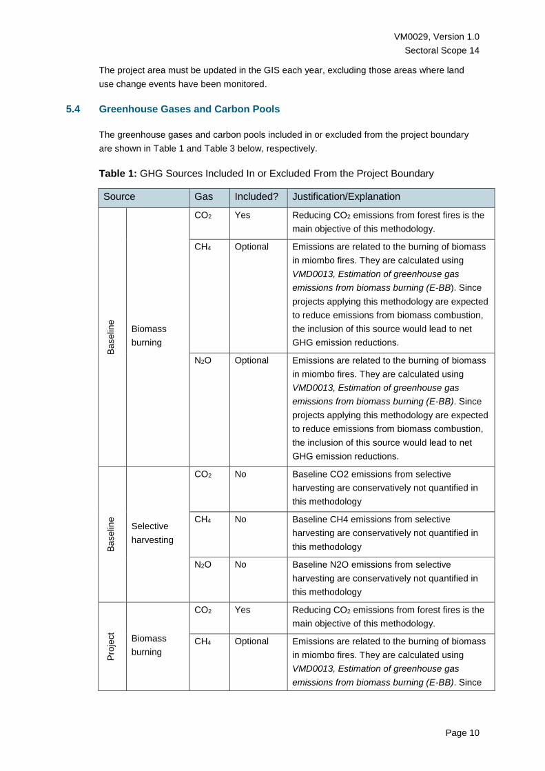
5.4 Greenhouse Gases and Carbon Pools

The greenhouse gases and carbon pools included in or excluded from the project boundary

are shown in Table 1 and Table 3 below, respectively.

Table 1: GHG Sources Included In or Excluded From the Project Boundary

Source Gas Included? Justification/Explanation

Baselin

e

Biomass

burning

CO2 Yes Reducing CO2 emissions from forest fires is the

main objective of this methodology.

CH4 Optional Emissions are related to the burning of biomass

in miombo fires. They are calculated using

VMD0013, Estimation of greenhouse gas

emissions from biomass burning (E-BB). Since

projects applying this methodology are expected

to reduce emissions from biomass combustion,

the inclusion of this source would lead to net

GHG emission reductions.

N2O Optional Emissions are related to the burning of biomass








Baselin

e

Selective

harvesting

CO2 No Baseline CO2 emissions from selective

harvesting are conservatively not quantified in

this methodology

CH4 No Baseline CH4 emissions from selective


this methodology

N2O No Baseline N2O emissions from selective


this methodology

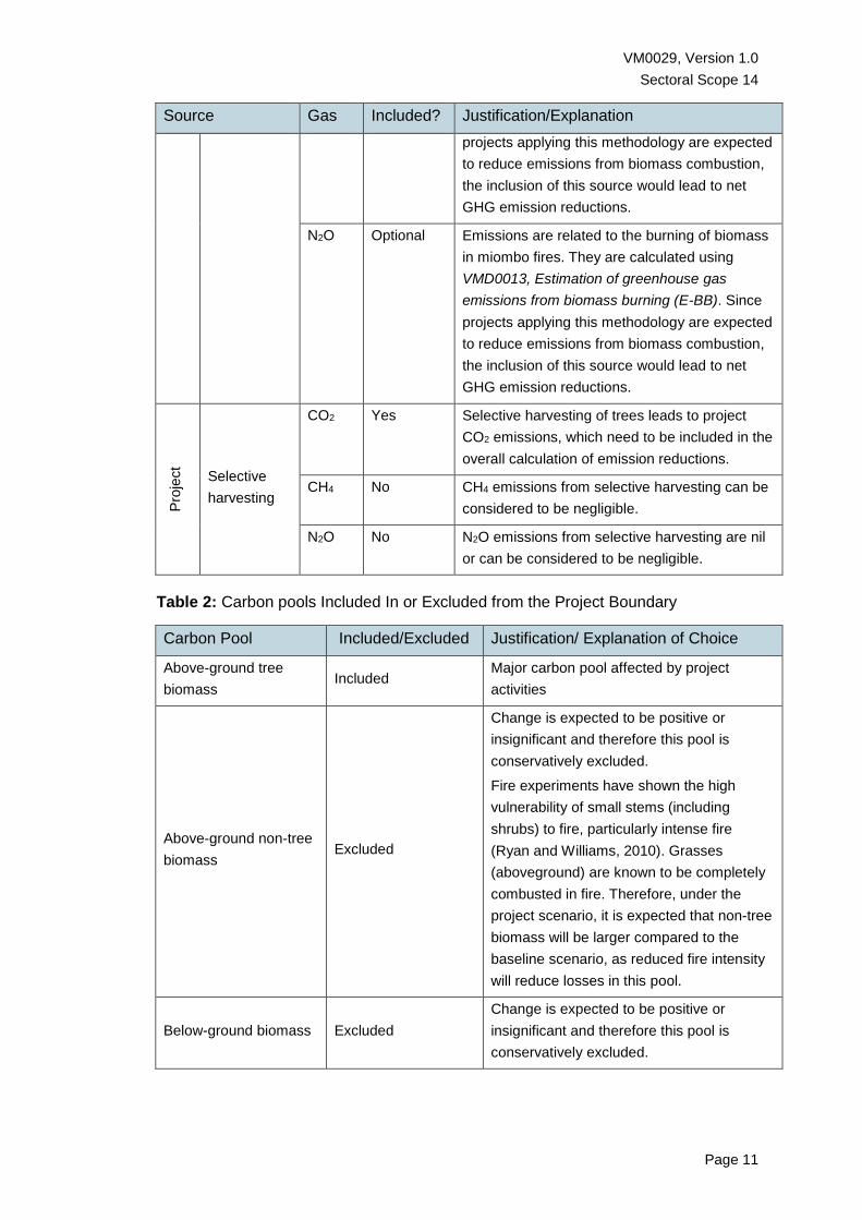
Pro

ject

Biomass

burning

CO2 Yes Reducing CO2 emissions from forest fires is the

main objective of this methodology.

CH4 Optional Emissions are related to the burning of biomass




VM0029, Version 1.0

Sectoral Scope 14

Source Gas Included? Justification/Explanation





N2O Optional Emissions are related to the burning of biomass








Pro

ject

Selective

harvesting

CO2 Yes Selective harvesting of trees leads to project

CO2 emissions, which need to be included in the

overall calculation of emission reductions.

CH4 No CH4 emissions from selective harvesting can be

considered to be negligible.

N2O No N2O emissions from selective harvesting are nil

or can be considered to be negligible.

Table 2: Carbon pools Included In or Excluded from the Project Boundary

Carbon Pool Included/Excluded Justification/ Explanation of Choice

Above-ground tree

biomass Included

Major carbon pool affected by project

activities

Above-ground non-tree

biomass Excluded

Change is expected to be positive or

insignificant and therefore this pool is

conservatively excluded.

Fire experiments have shown the high

vulnerability of small stems (including

shrubs) to fire, particularly intense fire

(Ryan and Williams, 2010). Grasses

(aboveground) are known to be completely

combusted in fire. Therefore, under the

project scenario, it is expected that non-tree

biomass will be larger compared to the

baseline scenario, as reduced fire intensity

will reduce losses in this pool.

Below-ground biomass Excluded




VM0029, Version 1.0

Sectoral Scope 14

Carbon Pool Included/Excluded Justification/ Explanation of Choice

Dead wood Excluded



conservatively excluded. See Section 5.3 of

Appendix 1 for further discussion.

Litter Excluded




Soil organic carbon Excluded




Wood products Included Carbon pool affected by project activities

6 BASELINE SCENARIO

The project proponent must apply Step 1 of the latest version of VT0001, Tool for the

Demonstration and Assessment of Additionality in VCS AFOLU Project Activities, which

results in a list of realistic and credible alternative land use scenarios to the project activity

and identifies the most plausible baseline scenario.

For the application of Step 1c of VT0001, the project proponent must apply the following

procedure:

Step 1. Barrier analysis. Taking the list of credible alternative land use scenarios resulting

from Step 1b of VT0001, a barrier analysis must be conducted to identify realistic and credible

barriers that prevent implementation of these land use scenarios following the procedures

described in Sub-step 3a of VT0001, mutatis mutandis. The project proponent must indicate

which of the alternative land use scenarios would face which identified barrier, and provide

verifiable information to support the presence of each particular barrier in relation to each

alternative land use scenario.

Step 2. Elimination of alternatives with barriers. Using the information in Step 1, eliminate

alternative land use scenarios that face a barrier to implementation. All land use scenarios

that face a barrier to implementation must be removed from the list. At least one viable

alternative land use scenario shall be identified.

Step 3. Selection of most plausible baseline scenario (if allowed by barrier analysis). Where

there is only one alternative land use remaining in the list, this alternative must be selected as

the most plausible baseline scenario. Where there is more than one alternative land use

remaining in the list, and one of these alternatives includes continuation of current land use

(ie, land use immediately prior to commencement of the project), continuation of current land

use must be chosen as the most plausible baseline scenario where the following conditions

are met:

1) The land manager(s) has not changed in the five years prior to the project start date;

VM0029, Version 1.0

Sectoral Scope 14

2) The current land uses have not changed in the five years prior to the project start date;

and

3) There have been no changes in mandatory applicable legal or regulatory requirements

during the five years prior to the project start date and no such changes are currently

under legal review by the relevant authorities.

Where there is more than one alternative land use remaining in the list and the most plausible

land use has still not been identified, proceed to Steps 4 and 5.

Step 4. Assess the profitability of alternative land use scenarios. Taking the list of alternative

land use scenarios resulting from Step 2 that face no barriers to implementation, document

the costs and revenues associated with each alternative land use and estimate the

profitability of each alternative land use. The profitability of alternative land uses must be

assessed in terms of the net present value (NPV) of net incomes over the project crediting

period. The key economic parameters and assumptions used in the analysis must be justified

in a transparent manner.

Step 5. Selection of most plausible baseline scenario (from profitability analysis). Select the

most profitable land use scenario from the analysis in Step 4 as the most plausible baseline

scenario.

Where the NPV of one or more of the alternative land use scenarios cannot be established,

and where all of the remaining alternative land use scenarios describe a land use where

carbon stocks are degraded equally or more severely relative to the current land use this

methodology conservatively assumes the baseline scenario to be the continuation of the

current land use only (ie, miombo vegetation subjected to carbon stock degradation by

anthropogenic fires, with the occurrence and intensity of fires equal to those observed in the

10 years before the start of the project activity). This assumption is conservative because:

Future carbon stock degradation as a result of anthropogenic fires is likely to increase

as the occurrence of fires is likely to increase due to population growth.

Not considering plausible alternative land use scenarios that include other causes of

forest degradation or deforestation leads to a higher estimate of baseline carbon

stocks and thus a lower estimate of a project’s GHG emission reductions and

removals.

Where the NPV of one or more of the alternative land use scenarios cannot be established,

and where one of these alternative land use scenarios is an anthropogenic activity which

increases carbon stocks or reduces carbon stock degradation relative to the pre-project land

use (eg, reforestation, enrichment planting or a reduction in fire occurrence and/or fire

intensity due to fire management or due to other anthropogenic causes such as a reduction in

population density), this methodology conservatively assumes this to be the most plausible

baseline scenario and, as per the applicability conditions of this methodology, the

methodology is not applicable.

VM0029, Version 1.0

Sectoral Scope 14

7 ADDITIONALITY

The project proponent must apply the latest version of VT0001 Tool for the Demonstration

and Assessment of Additionality in VCS AFOLU Project Activities.

8 QUANTIFICATION OF GHG EMISSION REDUCTIONS AND REMOVALS

8.1 Baseline Emissions

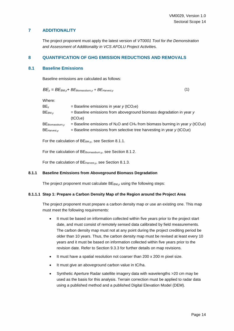
Baseline emissions are calculated as follows:

BEy = BEBM,y+ BEBiomassburn,y + BEHarvest,y (1)

Where:

BEy = Baseline emissions in year y (tCO2e)

BEBM,y = Baseline emissions from aboveground biomass degradation in year y

(tCO2e)

BEBiomassburn,y = Baseline emissions of N2O and CH4 from biomass burning in year y (tCO2e)

BEHarvest,y = Baseline emissions from selective tree harvesting in year y (tCO2e)

For the calculation of BEBM,y, see Section 8.1.1.

For the calculation of BEBiomassburn,y, see Section 8.1.2.

For the calculation of BEHarvest,y, see Section 8.1.3.

8.1.1 Baseline Emissions from Aboveground Biomass Degradation

The project proponent must calculate BEBM,y using the following steps:

8.1.1.1 Step 1: Prepare a Carbon Density Map of the Region around the Project Area

The project proponent must prepare a carbon density map or use an existing one. This map

must meet the following requirements:

It must be based on information collected within five years prior to the project start

date, and must consist of remotely sensed data calibrated by field measurements.

The carbon density map must not at any point during the project crediting period be

older than 10 years. Thus, the carbon density map must be revised at least every 10

years and it must be based on information collected within five years prior to the

revision date. Refer to Section 9.3.3 for further details on map revisions.

It must have a spatial resolution not coarser than 200 x 200 m pixel size.

It must give an aboveground carbon value in tC/ha.

Synthetic Aperture Radar satellite imagery data with wavelengths >20 cm may be

used as the basis for this analysis. Terrain correction must be applied to radar data

using a published method and a published Digital Elevation Model (DEM).

VM0029, Version 1.0

Sectoral Scope 14

The remote sensing data should be calibrated with field data as described in Section

9.3.1 below. If alternative field data is used, justification must be provided to show

how it is equivalent to or exceeds these requirements.

Miombo is typically a highly heterogeneous environment, so the carbon density map

may exhibit a lot of speckle complicating management. The map may be degraded in

resolution using any neutral algorithm so long as the pixel size is no more than 25

percent of the sample plots used to anchor it (50 percent limit in each direction).

A confidence interval must be calculated for the mean biomass across the entire map

using multiple random samples of calibration data to bootstrap the classification with

the remainder used to assess accuracy. The 95 percent confidence interval must be

no wider than 30 percent of the mean estimate.

The map may be extended beyond the scenes that have been calibrated by field data

by equalizing over scene overlaps, provided the neighboring scenes are broadly

similar in vegetation type and topography, and the confidence limit of the extended

map still meets the above criteria.

The map must include the project’s baseline reference region (BRR - see Step 3,

Section 8.1.1.3 below). Since the establishment of the BRR requires the use of the

carbon density map, an iterative process is necessary in which the carbon density

map is expanded until minimum requirements for the BRR are met.

8.1.1.2 Step 2: Stratify the Carbon Density Map

The first carbon density map of the project must be stratified into six strata, each covering a

range of 5 tC/ha and according to the stratification scheme presented in Table 3 below. The

lowest stratum (Stratum 1) may cover a range less than 5 tC/ha, and may start at any value

higher than 5 tC/ha, depending on the lower carbon density threshold as specified by the

forest definition the project proponent selects. If the threshold is higher than 5 tC/ha, then

Stratum 1 will start at the lower carbon density threshold for that forest definition, and extend

to the next multiple of 5. The median value for this stratum is the mid-point between the lower

and higher boundary values for the stratum. The next strata are then numbered

consecutively, with each covering a range of 5 tC/ha until the upper carbon density threshold

of 35 tC/ha is reached.

Subsequent revisions of the carbon density map may add new strata above 35 tC/ha, each

covering a range of 5 tC/ha. These new strata may only include project areas that were

previously below the maximum biomass allowable, but have since risen above that threshold.

Table 3: Range and Median Value (tC/ha) of the Six Carbon Density Strata

Stratum Range (tC/ha) Median carbon

density (tC/ha)

1 ≥5 and <10 7.5

2 ≥10 and <15 12.5

3 ≥15 and <20 17.5

VM0029, Version 1.0

Sectoral Scope 14

Stratum Range (tC/ha) Median carbon

density (tC/ha)

4 ≥20 and <25 22.5

5 ≥25 and <30 27.5

6 ≥30 and <35 32.5

8.1.1.3 Step 3: Delineate Project Area and BRR on the Carbon Density Map

All shape files of the project area must be overlaid onto the carbon density map. The shape

files must be updated each year a land manager is added to the project, and they must be

overlaid onto the most recent carbon density map. The project proponent must then

determine the area Ai,y of each stratum i within the project area in year y. This will be used in

equation (3) (Section 8.1.1.6).

The baseline reference region (BRR) is the region in which historical fire occurrence (baseline

fire history) data are collected. The BRR must be selected prior to the project start date and

remains fixed for the validity of the first carbon density map. A new BRR must be selected on

the most recent carbon density map at each revision of the baseline fire history (see

procedures specified in Section 9.3.4). The BRR may consist of multiple discreet areas. Areas

that meet the below criteria that are in closer proximity to the project area must take priority

over areas further away (ie, there must be no “cherry picking” of areas).

The project proponent may delineate more than one BRR to determine different baseline fire

histories for different portions of the project area. The project proponent must clearly indicate

which project areas have their baseline fire history determined by which BRR, and their

similarity in carbon density and fire history must be demonstrated per the requirements in this

section and Section 8.1.1.6.

The BRR must (at a minimum) incorporate:

1) All project areas presented in the project description, as well as any new areas that

are added in the future; and

2) Sufficient countable pixels within each biomass stratum to establish historical burn

probabilities (see Step 5, Section 8.1.1.5).

The project area must not be significantly different (at the 95 percent confidence level) in the

distribution of biomass from the BRR, as measured by the chi-squared goodness of fit

statistic, comparing the number of pixels in the project area in each biomass stratum with that

predicted by proportions in the BRR.

The project proponent must demonstrate that, for the areas inside the BRR, but outside the

project area, the following are true:

1) They are located within the Eastern Miombo ecoregion.

VM0029, Version 1.0

Sectoral Scope 14

2) They are covered with miombo woodland with aboveground carbon densities

between 5 tC/ha (unless otherwise specified by the forest definition selected by the

project proponent) and 35 tC/ha. All other areas (eg, agricultural areas, urban areas

and grasslands and woodlands/forest with carbon densities lower than 5 tC/ha and

higher than 35 tC/ha) must be excluded. The project proponent must use the carbon

density map prepared under Step 1 (Section 8.1.1.1) to delineate the BRR.

3) The main cause of carbon stock degradation in the BRR is anthropogenic fires. The

project proponent may use published or unpublished datasets, expert literature

sources or credible expert opinion to demonstrate this criterion.

4) The fire driving activities are similar and of similar relative importance to fire

occurrence as those in the project areas. The project proponent may use published or

unpublished datasets, expert literature sources or credible expert opinion to

demonstrate this criterion. Step 6 below addresses the quantitative similarity of the

fire history.

8.1.1.4 Step 4: Establish the Cut-Off Date between the Early Burning Season and the Late

Burning Season, and the Earliest Possible Burn Date and the End of the Burning

Season Date

The project proponent must specify an early burning season cut-off date between the early

burning seasons and late burning seasons, which must be used for both the baseline and

project scenarios. The cut-off date is the last day of the early burning season. It must be

specified by the project proponent prior to the project start date and remain fixed for the

project crediting period. The project proponent must use the default date of 30 June or

choose an alternative date supported by the credible opinion(s) of one or more experts with

demonstrable insights in miombo fire management and/or hands-on experience with fires in

the project region6.

The project proponent must also specify the earliest possible burn date that marks the

beginning of the early burning season. As with the cut-off date, it must be specified prior to

the project start date and remain fixed for the project crediting period. The project proponent

should use the day at the beginning of the dry season at which the monthly running average

rainfall (at least 10 years of data) first falls below 33 percent of peak wet season rainfall.

Alternatively, the project proponent may use the credible opinion(s) of one or more experts

with demonstrable insights in miombo fire management and/or hands-on experience with fires

in the project region to justify an alternative earliest possible burn date.

Finally, the project proponent must establish the end of burning season date that marks the

end of the dry season. As with the cut-off date, it must be specified by the project proponent

prior to the project start date and remain fixed for the project crediting period. The project

proponent should use the day at the end of the dry season at which the monthly running

average rainfall (at least 10 years of data) first rises above 33 percent of peak wet season

rainfall. Alternatively, the project proponent may use the credible opinion(s) of one or more

6 Suitable experts include, but are not limited to, local government officials and ecological researchers. The

project proponent may additionally choose to consult international experts in large scale early burning.

VM0029, Version 1.0

Sectoral Scope 14

experts with demonstrable insights in miombo fire management and/or hands-on experience

with fires in the project region to justify an alternative end of burning season date.

8.1.1.5 Step 5: Determine Historic Burn Probabilities for Each Stratum in the BRR (Fire

History)

Sub-step 5.1. The baseline fire frequencies are determined from a fire history that must be

derived at the outset of the project, as set out below. Every 10 years the fire history must be

revalidated as set out in Section 9.3.4 below.

To construct the initial fire history, the project proponent must gather as many early- and late

season burn observations as possible for the entire BRR for the historical 10-year period

before the project start date or, for each revision of the fire history baseline (see Section

9.3.4), said observations must be gathered for the historical 10-year period before the revision

date. The project start date may not be delayed by more than 5 years beyond the last year of

the historical 10-year period.

The project proponent must:

1) Collect composite satellite observations for the BRR from medium resolution (ie, 10s

of meter pixels) images (such as Landsat or SPOT) using spectral indices as a proxy

for fire occurrence, and group them for each of the 10 years. Images from before the

earliest possible burn date, or from more than three months after the end of burning

season date, must be excluded. There must be no systematic bias in the selection of

images. Where feasible, all available images in that time period from the selected

source should be analyzed.

2) Apply a burned area detection algorithm to determine where a fire has occurred (eg,

the spectral index method as described in Bastarrika, 2011). This must be performed

for all cloud-free pixels on the available images (ie, no “cherry picking”). Create the

burn scar dataset according to the following procedure:

a) Satellite imagery should undergo atmospheric correction, cloud masking and

conversion to an estimate of surface reflectance, where appropriate.

b) Where appropriate, a series of spectral indices should be calculated which

highlight the reflective properties of burn scars (eg, NDVI, GEMI, MIRBI). In

addition to aiding classification, use of these indices mitigates against the effects

of varying illumination, acquisition geometries and topographic effects in satellite

imagery.

c) A training dataset of burned and unburned areas must be manually identified in

remote sensing imagery by a competent operator. The operator must have

access to all available satellite imagery. This dataset must include classified

pixels across a number of images, spanning different localities, land cover types,

seasons and years. The training data must be developed conservatively, with

only the central parts of burn scars (where there can be no doubt) labeled as

burned in the training data. This data set must be preserved as evidence of

conservativeness.

VM0029, Version 1.0

Sectoral Scope 14

d) The likelihood of a burn must be computed for each usable pixel in each image

using a supervised image classification algorithm. The classifier derivation should

incorporate a variable sparsity preference to avoid over-fitting. The classification

should be carried out as a cross-validation, and boot-strapped with a part of the

training data used to guide the classifier, and the remaining training data used to

assess accuracy. A consistent average classification accuracy of >95 percent is

required for acceptance of the classification algorithm.

e) Where the status of a pixel is ambiguous, the classifier must use a conservative

minimum threshold of burn likelihood (at least 60 percent7) when registering a

pixel as burned.

f) The earliest burn scar observation of a pixel in a given year disqualifies any

subsequent observations of the same pixel in that year from further consideration

in the analysis.

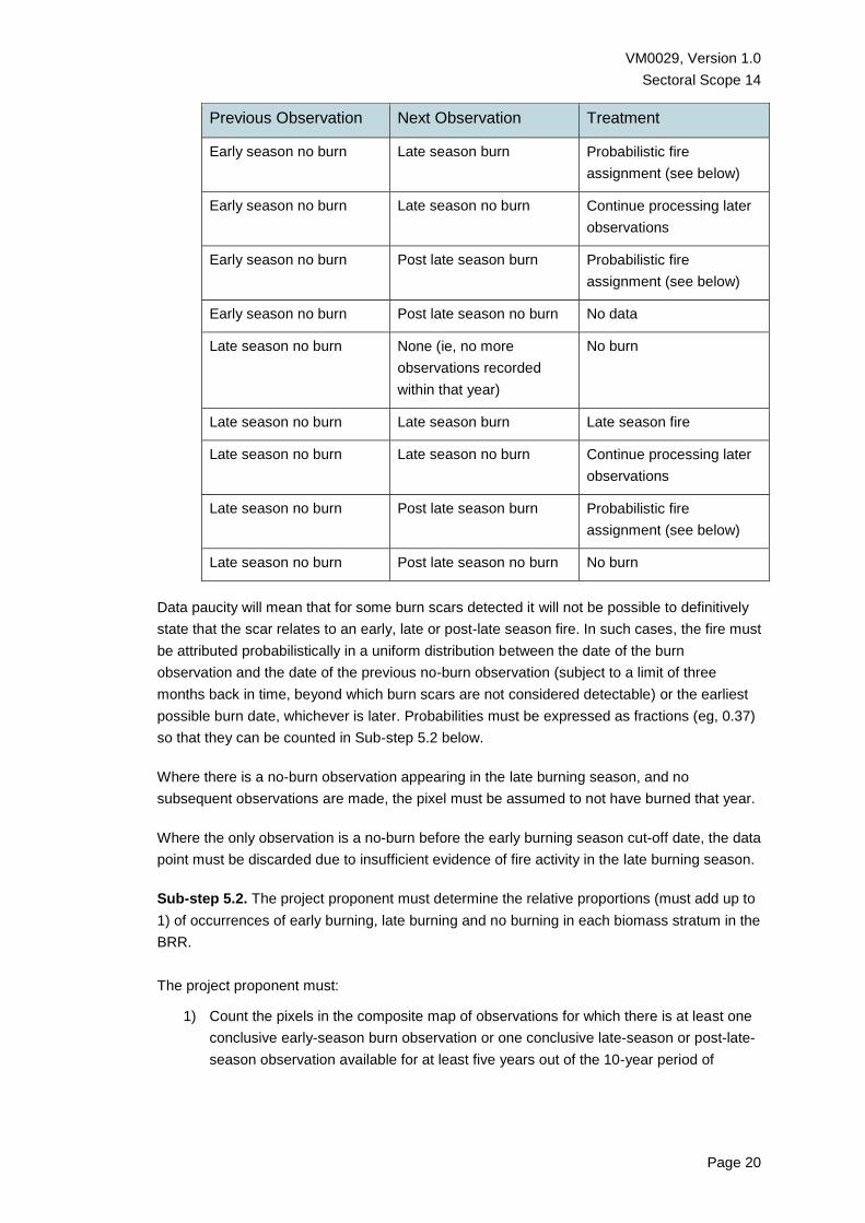
3) Attribute each observed burn scar to a burn in the early burning season or the late

burning season using the date of the observation, according to table 5 below.

Table 5: Burn Scar Attribution

Previous Observation Next Observation Treatment

None None (ie, no observations

recorded within that year)

No data

None Early season burn Early season fire

None Early season no burn Continue processing later

observations

None Late season burn Probabilistic fire

assignment (see below)

None Late season no burn Continue processing later

observations

None Post late season burn Probabilistic fire


None Post late season no burn No data

Early season no burn None (ie, no more

observations recorded

within that year)

No data

Early season no burn Early season burn Early season fire

Early season no burn Early season no burn Continue processing later

observations

7 Giglio et al (2009) empirically determined that the posterior probability of detection should be at least 0.6 to

minimise the frequency of commission errors.

VM0029, Version 1.0

Sectoral Scope 14

Previous Observation Next Observation Treatment

Early season no burn Late season burn Probabilistic fire


Early season no burn Late season no burn Continue processing later

observations

Early season no burn Post late season burn Probabilistic fire


Early season no burn Post late season no burn No data

Late season no burn None (ie, no more

observations recorded

within that year)

No burn

Late season no burn Late season burn Late season fire

Late season no burn Late season no burn Continue processing later

observations

Late season no burn Post late season burn Probabilistic fire


Late season no burn Post late season no burn No burn

Data paucity will mean that for some burn scars detected it will not be possible to definitively

state that the scar relates to an early, late or post-late season fire. In such cases, the fire must

be attributed probabilistically in a uniform distribution between the date of the burn

observation and the date of the previous no-burn observation (subject to a limit of three

months back in time, beyond which burn scars are not considered detectable) or the earliest

possible burn date, whichever is later. Probabilities must be expressed as fractions (eg, 0.37)

so that they can be counted in Sub-step 5.2 below.

Where there is a no-burn observation appearing in the late burning season, and no

subsequent observations are made, the pixel must be assumed to not have burned that year.

Where the only observation is a no-burn before the early burning season cut-off date, the data

point must be discarded due to insufficient evidence of fire activity in the late burning season.

Sub-step 5.2. The project proponent must determine the relative proportions (must add up to

1) of occurrences of early burning, late burning and no burning in each biomass stratum in the

BRR.

The project proponent must:

1) Count the pixels in the composite map of observations for which there is at least one

conclusive early-season burn observation or one conclusive late-season or post-late-

season observation available for at least five years out of the 10-year period of

VM0029, Version 1.0

Sectoral Scope 14

analysis8. A conclusive observation means no data are missing and it is not obscured

by clouds. Post-late season observations may be made up to 3 months after the end

of burning season date. These are the countable pixels in the composite map.

2) Overlay the countable pixels onto the carbon density map and attribute each

countable pixel to a biomass stratum. Countable pixels must cover at least 50 percent

of the area of each biomass stratum within the BRR.

3) For each year in the 10-year period in each biomass stratum, count the countable

pixels that burned in the early burning season, that burned in the late burning season

and that observably did not burn in either period. Include fractions (resulting from the

probabilistic attribution described in Sub-step 5.1, step 4c above) in the count.

4) For each biomass stratum, sum up the yearly totals of countable pixels that burned in

the early burning season for the 10-year period. The project proponent must do the

same for those countable pixels which burned in the late burning season and those

which did not burn in either period.

5) For each biomass stratum, calculate the proportion of the total number of pixels that

burned in the early burning season over the total number of pixels for the 10-year

period for which there is observational evidence, as follows:

BLPROBEarlyburn,i = ∑CountEarlyburni,y / ∑CountPixi,y (2)

Where:

BLPROBEarlyburn,i = Baseline probability of early burning occurring in stratum i (fraction)

CountEarlyburni,y = Number of countable pixels in stratum i in year y that showed a

burn scar in the early burning season

CountPixi,y = Number of countable pixels in stratum i in year y

The project proponent must use Equation (2) to calculate BLPROBLateburn,i and

BLPROBNoburn,i, mutatis mutandis. BLPROBEarlyburn,I, BLPROBLateburn,i and BLPROBNoburn,i must

be input in the GapFire model as the baseline relative probabilities of early burning, late

burning and no burning for that stratum.

8.1.1.6 Step 6: Demonstrate the Project Area And BRR Have Similar Fire Baseline Histories

Step 3 above requires the project area and BRR to be qualitatively similar, and quantitatively

similar in respect to biomass. To avoid any biases, they must also exhibit similar fire histories.

Many variables affect the frequency of fires and their spread, including accessibility

(infrastructure), distance from human settlements and various aspects of topography (hilliness

8 Based on Archibald et al., 2013 it can be established that most areas in the Eastern Miombo ecoregion burn at

least once every two years. Therefore, if five years of observations are available this will provide sufficient data

to conclusively establish baseline burn occurrences. Five years is also suggested as a period of sufficient

observations by ESA, 2011.

VM0029, Version 1.0

Sectoral Scope 14

and slope). Rather than assessing each of these in turn, the project proponent must

demonstrate that the resulting fire histories as detected above are not statistically dissimilar.

The primary sensitivity of the GapFire model is late season burn rate (see Appendix 1 for

further explanation), so it is this variable that must be demonstrably similar (ie, for the

purposes of this test, an early burn is treated the same as a no burn). To assess this

similarity, the expected late season burn rates must be computed for each stratum as shown

in Table 6 below.

Table 6: Expected Late Season Burn Rates

Stratum Expected Burned Pixels Expected Un-burned Pixels

1 NPPA,1 × BLPROBLateburn,1 NPPA,1 × (1 - BLPROBLateburn,1)

2 NPPA,2 × BLPROBLateburn,2 NPPA,2 × (1 - BLPROBLateburn,2)

3 … …

4 … …

5 … …

6 … …

Where:

NPPA,i = total number of pixels in the project area in stratum i

BLPROBLateburn,i = Baseline probability of late burning occurring in stratum i (as determined

in Step 5 above)

These expected burn rates must be compared with actual burn rates in the project area using

the chi-squared goodness of fit statistic on 11 degrees of freedom (+2 for each additional

stratum) at the 90 percent confidence level. This analysis of similarity must be performed for

the entire project area each time the project area is adjusted (eg, when new project activity

instances are added). Where more than one BRR has been specified, each discreet area of

the new project activity instance must be coupled to one BRR.

Where the chi-squared test does not show significant differences between the project area

and the BRR, the baseline fire history as determined in Step 5 may be used. If the chi-

squared test is failed, project proponents have two options: (1) modify the baseline fire history

and/or (2) modify the BRR.

Option A: modify the baseline fire history to use the most conservative history This must be

implemented on a per stratum basis. Where BLPROBLateburn,i for the BRR is higher than in the

project area, the lower figure from the project area should be used. Where BLPROBLateburn,i for

the BRR is lower than in the project area, no modification is necessary because the fire

history in the BRR is more conservative than in the project area. Where this is the case for all

strata, no actual modification is necessary, and the fire history as given for the BRR should be

used.

Option B: Modify The BRR, by either adjusting the Boundaries and/or Splitting It. The BRR

may only be modified when the baseline fire history is revised (as per Section 9.3.4). At such

times project proponents may amend the boundaries in order to derive a new BRR that

VM0029, Version 1.0

Sectoral Scope 14

passes the chi-squared test of fire history similarity. Project proponents may also choose to

split the BRR and project area into paired multiple project activity instances (see Section

8.1.1.3). The analysis of similarity must be repeated and passed for each BRR and

corresponding project area separately.

If the project proponent is adding one or more new project activity instances to a grouped

project, and this change causes the similarity test to fail, the project proponent must establish

one or more new BRRs paired only with the new activity instances.

8.1.1.7 Step 7: Run the Gapfire Model and Determine Baseline Emissions from Aboveground

Biomass Degradation Due To Fire

Sub-step 7.1. The baseline early burning probability, late burning probability and no burning

probability for each stratum must be entered into the GapFire model, thereby creating a

separate GapFire file for each stratum. These baseline inputs into the model remain fixed for

the validity of the baseline fire history, and must be updated every time the baseline fire

history is revised. The median carbon density for the stratum (from Table 4) must also be

entered. The model must be run with at least 100,000 patches9. See Annex 1 for a detailed

description of the GapFire model including a brief user manual (Annex 1, Section 5). The

project proponent must repeat this step for each stratum.

Note the model will calculate the baseline and project scenarios simultaneously. Project

scenario inputs are the early burning probability, late burning probability and no burning

probability as monitored each year by the project proponent (see Section 9.2).

Sub-step 7.2. Calculate annual baseline emissions from aboveground biomass degradation

for the project by applying Equation (3) (ie, by multiplying the hectares in each stratum with

the baseline average annual carbon stock changes per hectare over the first 10 years of the

simulation).

BEBMy = ∑((BBMCi,sy=0 – BBMC i,sy=10)/10 × Ai,y × 44/12) (3)

Where:

BEBMy = Baseline emissions from aboveground biomass degradation in year y

(tCO2e)

BBMCi,sy=0 = Carbon stored in aboveground biomass per hectare in stratum i in GapFire

simulation year 0 in the baseline scenario (tC/ha)

BBMCi,sy=10 = Carbon stored in aboveground biomass per hectare in stratum i in GapFire

simulation year 10 in the baseline scenario (tC/ha)

Ai,y = Area of stratum i in year y within the project area (ha)

44/12 = Conversion factor from tC into tCO2e

9 This amount of patches comfortably deals with output variability of individual patches in the GapFire model (see

Appendix 1) and ensures a smooth output curve.

VM0029, Version 1.0

Sectoral Scope 14

8.1.2 Baseline Emissions from Biomass Burning

Baseline emissions from biomass burning are calculated using the latest version of the VCS

module VMD0013 Estimation of greenhouse gas emissions from biomass and peat burning

(E–BPB) equation 1 of VMD0013 (Aburn,i,t * Bi,t * COMFi) must be substituted with the term (Ai,y

* (AvCMortBLi,y / CF)), such that the equation reads:

BEBiomassburn,y = ∑(Ai,y × (AvCMortBLi,y / CF) × Gg × 10-3 × GWPg) (4)

Where:

BEBiomassburn,y = Baseline emissions of N2O and CH4 from biomass burning in year y

(tCO2e)


AvCmortBLi,y = Average annual carbon stored in biomass dying as a result of tree

mortality over the first 10 years’ output of the annual GapFire model

baseline simulation for stratum i (see Section 8.1.1.7) (tC/ha)

CF = Carbon fraction of woody biomass (dimensionless)

Gg = Emission factor for gas g; kg t-1 dry matter burnt

GWPg = Global warming potential for gas g; t CO2/t gas g

g =1, 2, 3 … Greenhouse gases

The adaptation of equation 1 of VMD0013 calculates baseline emissions from biomass

burning for each stratum based on the baseline biomass mortality in year y (the average over

a 10-year period is taken), as calculated by the GapFire model. This approach assumes direct

emissions of non-CO2 gases from mortality, rather than from the dead wood pool.

8.1.3 Baseline emissions from selective tree harvesting

Baseline emissions from selective tree harvesting are conservatively not quantified.

Therefore:

BEHarvest,y = 0 (5)

8.2 Project Emissions

Project emissions are calculated as follows:

PRy = PRBM,y + PEBiomassburn,y + PEHarvest,y (6)

Where:

PRy = Project emissions in year y (tCO2e)

PRBM,y = Project emissions from aboveground biomass in year y (tCO2e)

PEBiomassburn,y = Project emissions of N2O and CH4 from biomass burning in year y (tCO2e)

PEHarvest,y = Project emissions from selective tree harvesting in year y (tCO2e)

For the calculation of PRBM,y, see Section 8.2.1.

VM0029, Version 1.0

Sectoral Scope 14

For the calculation of PEBiomassburn,y, see go to Section 0.

For the calculation of PEHarvest,y, see Section 8.2.3.

8.2.1 Project Emissions from Aboveground Biomass

The project proponent must calculate PRBM,y using the following steps:

8.2.1.1 Step 1: Calculate the Probabilities of Early Burning, Late Burning and No Burning

The project proponent must calculate the probabilities of early burning, late burning and no

burning by applying Equation 7 below.

PRPROBEarlyburn,y = ∑(FFEarlyburn,z,y × Areaz,y) / ∑( Areaz,y) (7)

Where:

PRPROBEarlyburn,y = Project probability of early burning in year y (fraction)

FFEarlyburn,z,y = Early burning fire frequency in FMU z in year y (%)

Areaz,y = Area of FMU z in year y (ha)

The project proponent must use Equation 7 to calculate PRPROBLateburn,y and

PRPROBNoburn,y, mutatis mutandis.

Note that PRPROBEarlyburn,y, PRPROBLateburn,y and PRPROBNoburn,y are (for practical and cost-

saving reasons) not broken down per biomass stratum. This is permitted so long as the

monitoring data is representative of the forests within the project area (as is required by

Section 9.3 below)10.

8.2.1.2 Step 2: Run the Gapfire Model and Determine Project Emissions

Sub-step 1.1. The project proponent must enter the monitored early burning probability, late

burning probability and no burning probability (they are identical for each stratum) into the

entry table in each GapFire model file prepared for each strata in Section 8.1.1.6. The model

must start its simulation in the year of the satellite images utilized for the preparation of the

most recent carbon density map. Where this date is before the project start date, the project

proponent must enter baseline burn probabilities for the years before the project start date.

Each file must be run with at least 100,000 patches. Repeat this step for each stratum.

Sub-step 1.2. Based on the most recent carbon density map (see Section 8.1.1.1), the

project proponent must determine the number of hectares within each stratum. This must be

updated each time the project area is expanded.

10 This approach is conservative because analysis of the GapFire model showed that emission reductions and

removals from fire management increase in a linear manner with increasing biomass, while burn probabilities

decrease with increasing biomass. Therefore, by monitoring the average burn probabilities across the strata and

inputting these into the model, the burn probabilities in the higher biomass strata are over-estimated; these strata

are where a lower burn probability would have yielded the highest emission reductions and removals.

VM0029, Version 1.0

Sectoral Scope 14

Sub-step 1.3. The project proponent must calculate the current total project carbon stock by

applying Equation 8 below.

CCSBM,y = ∑((PBMCi,y × Ai,y ) – (Adeg – Areg) × 5 (8)

Where:

CCSBM,y = Current total carbon stocks in the aboveground biomass pool in year y (tC)

PBMCi,y = Carbon stored in aboveground biomass per hectare in stratum i in GapFire

simulation year y in the project scenario (tC/ha)


Adeg = Project areas that degrade below 5tC/ha due to carbon map revision (ha)

Areg = Project areas that regenerate above 5tC/ha due to carbon map revision

(ha)

Sub-step 1.4. The project proponent must calculate the annual project carbon stock changes

for the project by applying Equation 9 below.

PRBM,y = (CCSBM,y – CCSBM,y-1) × 44/12 (9)

Where:

PRBM,y = Project removals or emissions from forest biomass regeneration or

degradation in the aboveground biomass pool in year y (tCO2e)

CCSBM,y = Current total carbon stocks in the aboveground biomass pool in year y (tC).


8.2.2 Project Emissions from Biomass Burning

The project proponent must calculate project emissions from biomass burning using the latest

version of the VMD0013, Estimation of greenhouse gas emissions from biomass burning (E-

BB). Equation 1 of VMD0013 (Aburn,i,t × Bi,t × COMFi) must be substituted with the term Ai,y *

(AvCMortPRi,y * / CF), such that Equation 1 reads:

PEBiomassburn,y = ∑(Ai,y × (AvCMortPRi,y / CF) × Gg,i × 10-3 × GWPg) (10)

Where:

PEBiomassburn,y = Project emissions of N2O and CH4 from biomass burning in year y

(tCO2e)


AvCmortPRi,y = Average yearly carbon stored in biomass dying as a result of tree

mortality over the first 10 years’ output of the yearly GapFire model

project simulation for stratum i (see Section 8.1.1.7) (tC/ha)

CF = Carbon fraction of woody biomass (dimensionless)

Gg,i = Emission factor for stratum i for gas g; kg t-1 dry matter burnt

GWPg = Global warming potential for gas g; t CO2/t gas g

g =1, 2, 3 ... Greenhouse gases

VM0029, Version 1.0

Sectoral Scope 14

This adaptation of Equation 1 of VMD0013 calculates project emissions from biomass burning

for each stratum based on the project biomass mortality in year y (the average over a 10-year

period is taken), as calculated by the GapFire model. This approach assumes direct

emissions of non-CO2 gases from mortality, rather than from the dead wood pool.

8.2.3 Project Emissions from Selective Tree Harvesting

Where selective harvesting occurs in the project, the associated emissions must be

quantified. The project description must describe how harvesting is managed, and specify

how it will be monitored to ensure sustainability (ie, that harvested biomass is not greater than

regeneration capacity) using industry standard measures such as annual allowable cut and

mean annual increment.

PEharvest,y = PEwoodproc,y + PEMT, y-21 to y-1 (11)

Where:

PEharvest,y = Project emissions from selective tree harvests in year y (tCO2e)

PEwoodproc,y = Project emissions from wood processing in year y (tCO2e). Assumes all

wood is processed in year of harvesting (must be calculated using the

method in either Section 8.2.3.1 or Section 8.2.3.2).

PEMT, y-21 to y-1 = Project emissions from the medium-term wood products pool (remaining

in this pool between 3 and 100 years)

8.2.3.1 Calculation of Project Emissions from Wood Processing Based On Bole Volume

PEwoodproc,y = ∑(HVj,y × (WasteFactor + BEF – 1) × WDj × CF × 44/12) (12)

Where:

PEwoodproc,y = Project emissions from wood processing in year y (tCO2e)

HVj,y = Harvested bole volume of species j in the project area in year y (m3) –

monitored

WasteFactorj = Fraction of harvested volume effectively emitted to the atmosphere during

wood processing. Default is 0.2411.

BEF = Biomass expansion factor (dimensionless). Ratio of aboveground biomass

to biomass of bole volume.

WDj = Wood density of harvested species j (t/m3)

CF = Carbon fraction of woody biomass (default =0.47)12 (dimensionless)


11 Winjum et al., 1998.

12 IPCC, 2006

VM0029, Version 1.0

Sectoral Scope 14

8.2.3.2 Calculation of Project Emissions from Wood Processing Based On Tree Volume

PEwoodproc,y = ∑(TTVj(Dj,y) × ((WasteFactorj / BEF) + BEF – 1) × WDj ×

CF × 44/12) (13)

Where:

PEwoodproc,y = Project emissions from selective tree harvests in year y (tCO2e)

TTVj(D,j,y) = Total volume of harvested trees of species j, calculated using an allometric

equation or table derived from recognized independent source (eg,

government volume tables). The input variable of such equation must be the

diameter of each tree harvested (Dj,y) of species j in the project area in year

y (cm).

WasteFactorj = Fraction of harvested volume effectively emitted to the atmosphere during

wood processing. Default is 0.2413.

BEF = Biomass expansion factor (dimensionless). Ratio of aboveground biomass

to biomass of bole volume.




8.2.3.3 Calculation of Project Emissions from the Medium-Term Wood Products Pool

PEMT, y = VEMT,j,y × WDj × CF × 44/12 (14)

VEMT,j,y = (VMT,j,y-21 + VMT,j,y-20 + VMT,j,y-19 + …. + VMT,j,y-1) /20 (15)

Where:

PEMT, y-21 to y-1 = Project emissions from the medium-term wood products pool (remaining in

this pool between 3 and 100 years)

VEMT,j,y = Volume of species j in year y in the medium-term wood products pool

(remaining in this pool between 3 and 100 years) that is emitted each year

VMT,j,y = Volume of species j in year y that enters the medium-term wood products

pool (remaining in this pool between 3 and 100 years)




13 Winjum et al., 1998

14 IPCC (2006)

15 IPCC (2006)

VM0029, Version 1.0

Sectoral Scope 14

8.3 Leakage

The project description must present an estimate of activity shifting leakage that takes into

account all fire driving activities. The estimate must be based on interviews, rural appraisals

and/or other local expert knowledge.

The matrix computation outlined in Section 8.3.1 below must be used for the purpose of

estimating the proportion of the project area that is burned outside of the project area from the

shifting of fire driving activities. The estimate must be revalidated every 10 years.

The procedure in Section 8.3.2 calculates estimated leakage emissions. This leakage

calculation must be done every year. Total estimated leakage that is equal to or higher than 5

percent of the project’s overall emission reductions and removals must be subtracted in the

final calculation of net emission reductions and removals in Section 8.4.

8.3.1 Matrix Computation of Fire Driving Activity Leakage

The extent of the area burned outside the project area as a result of shifting fire driving

activities (ABADm,fc) must be quantified by completing the matrix below (Table 7). Cells that

are calculated are shaded in light grey; cells that require input have no shading. Every cell is

a percentage value. The matrix must be completed using the steps below:

1) List the months of the dry season across the top.

2) Enter the fire frequency for each month from the baseline fire history in the cells

labeled BBRm% where m is the month number.

3) Compute for each month the cumulative baseline burn rate (the sum of all burn rates

up to and including that month), and the future burn rate (the likelihood that area not

burned already will be burned later in the year).

4) List the different causes of fires, and for each month insert the estimated proportion of

fires started by that cause (FSm,fc,) weighted by area affected. These must sum to 100

percent for each month, and must be obtained from interviews, rural appraisals

and/or other local expert knowledge.

5) List the different rates of fire displaceability (Dfc,) according to cause of fire as

determined from interviews, rural appraisals and other local expert knowledge (not

expected to vary by month).

6) Calculate, for each month and cause of fire, the resulting expected proportion of fires

that will be displaced (FDm,fc).

7) Calculate the total displacement of burned area for each month and cause of fire

(BADm,fc)

8) Reduce BADm,fc by the proportion FBBRm that would burn in the future in the absence

of the project.

9) The resulting proportion (ABADm,fc,) is the additional area that will be burned in month

m as a result of cause of fire fc, as a proportion of the project area. Summing across

all months and causes of fires produces a final estimate of the proportion of the total

project area affected by fire driving activity leakage in any given year.

VM0029, Version 1.0

Sectoral Scope 14

Table 7: Matrix table for calculating the extent of the area burned outside the project

area as a result of shifting fire driving activities

Month May June … Oct Nov Overall

Baseline Burn Rate BBR1% BBR2% … BBR6% BBR7% ∑ BBR

Cumulative BBR CBBRm = ∑ BBR𝑖

m

1

… …

Future BBR FBBRm = ∑ BBR − CBBRm … …

Fire Causes

FC1 FS1,1% FS2,1% … FS6,1% FS7,1%

FC2 FS1,2% FS2,2% … FS6,2% FS7,2%

… … … … … …

FCn FS1,n% FS2,n% … FS6,n% FS7,n%

Total ∑ FS1,fc

n

1

= 100% … … …

Displaceability

FC1 D1%

FC2 D2%

… …

FCn Dn%

Fires Displaced

FC1 FD1,1% = FS1,1% x D1% … FD6,1% = FS6,1% x D1%

FC2 FD1,2% = FS1,2% x D2% … FD6,2% = FS6,2% x D2%

… … … … … …

FCn FD1,n% = FS1,n% x Dn% … FD6,n% = FS6,n% x Dn%

Burned Area Displaced

FC1 BAD1,1% = FD1,1% x BRR1% … BAD6,1% = FD6,1% x

BRR6% ∑ BADm,1

m

VM0029, Version 1.0

Sectoral Scope 14

Month May June … Oct Nov Overall

FC2 BAD1,2% = FD1,2% x BRR1% … BAD6,2% = FD6,2% x

BRR6% ∑ BADm,2

m

… … … … … … …

FCn BAD1,n% = FD1,n% x BRR1% … BAD6,n% = FD6,n% x

BRR6% ∑ BADm,n

m

Total ∑ BAD1,fc

fc

∑ BAD2,fc

fc

… ∑ BAD6,fc

fc

∑ BAD7,fc

fc

∑ BADm,fc

m,fc

Adjusted Burned Area Displaced (less what would have burned any way)

FC1 ABAD1,1% = BAD1,1% x (1 -

CBRR1%)

… … ∑ ABADm,1

m

FC2 … ABAD2,m% = BAD2,m% x (1 -

CBRR2%)

… ∑ ABADm,2

m

… … … … … … …

FCn … … ABADn,7% = BADn,7% x (1 -

CBRR7%) ∑ ABADm,n

m

Final Total ∑ ABAD1,fc

fc

∑ ABAD2,fc

fc

… ∑ ABAD6,fc

fc

∑ ABAD7,fc

fc

∑ ABADm,fc

m,fc

8.3.2 Calculation of Leakage Emissions

LFDA,y = ∑Ai,y × ∑ABADm,fc × LEFnoburn-to-lateburn (16)

Where:

LFDA,y = Leakage emissions from shifting of fire driving activities in year y (tCO2e)


ABADm,fc = Area additionally burned (that would not otherwise have burned) outside the

project area as a result of the shifting of fire driving activities in month m as a

result of cause of fire fc, expressed as a proportion of the project area (from

Section 8.3.1) (%)

LEFnoburn-to-lateburn = Leakage emission factor of areas additionally burned (that would not

otherwise have burned) as a result of the shifting of fire driving activities

(tCO2e/ha)

LEFnoburn-to-lateburn must be calculated using the following steps:

1) Based on the carbon density map (Section 8.1.1.1), determine the average carbon

density (tC/ha) within the BRR (the assumption is made that fire driving activities

would be shifted into the BRR).

VM0029, Version 1.0

Sectoral Scope 14

2) Prepare a separate GapFire file for the calculation of LEFnoburn-to-lateburn, that starts its

simulation at the average carbon density determined in Step 1. Enter as the baseline

burn probabilities: 100 percent no burn, 0 percent early burn and 0 percent late burn.

Enter as the project burn probabilities: 0 percent No burn, 0 percent early burn and

100 percent late burn. Run the model with at least 100,000 patches.

3) Based on the GapFire output, calculate LEFnoburn-to-lateburn as follows:

LEFnoburn-to-lateburn = ((BBMCi,y-1 – BBMC i,y) – (PBMCi,y-1 – PBMC i,y))

× 44/12

(17)

Where:

LEFnoburn-to-lateburn = Leakage emission factor of areas additionally burned (that would not

otherwise have burned) as a result of the shifting of fire driving activities

(tCO2e/ha)

BBMCi,y = Carbon stored in aboveground biomass per hectare in GapFire simulation

year y in stratum i in the baseline scenario (tC/ha)

PBMCi,y = Carbon stored in aboveground biomass per hectare in GapFire simulation

year y in stratum i in the project scenario (tC/ha)


8.4 Net GHG Emission Reductions and Removals

Net GHG emission reductions and removals are calculated as follows:

NERRy = PRy – BEy – LFDA,y (18)

Where:

NERRY = Net GHG emissions reductions and removals in year y (tCO2e)

PRy = Project net removals or emissions in year y (tCO2e)

BEY = Baseline emissions in year y (tCO2e)

LFDA,y = Leakage emissions in year y (tCO2e)

The number of VCUs to be issued to a project in year y is calculated as follows:

VCUy = NERRy – EDMUy – BufferDiscounty (19)

BufferDiscounty = (BEBM,y – PRBM,y) × RFy (20)

Where:

VCUy = Number of VCUs to be credited to a project in year y

NERRY = Net GHG emissions reductions and removals in year y (tCO2e)

EDMUy = Emissions Detected at Map Update in year y (tCO2e) as specified in

Section 9.3.4 (expected to be zero)

BEBM,y = Baseline emissions from aboveground biomass degradation in year y

(tCO2e)

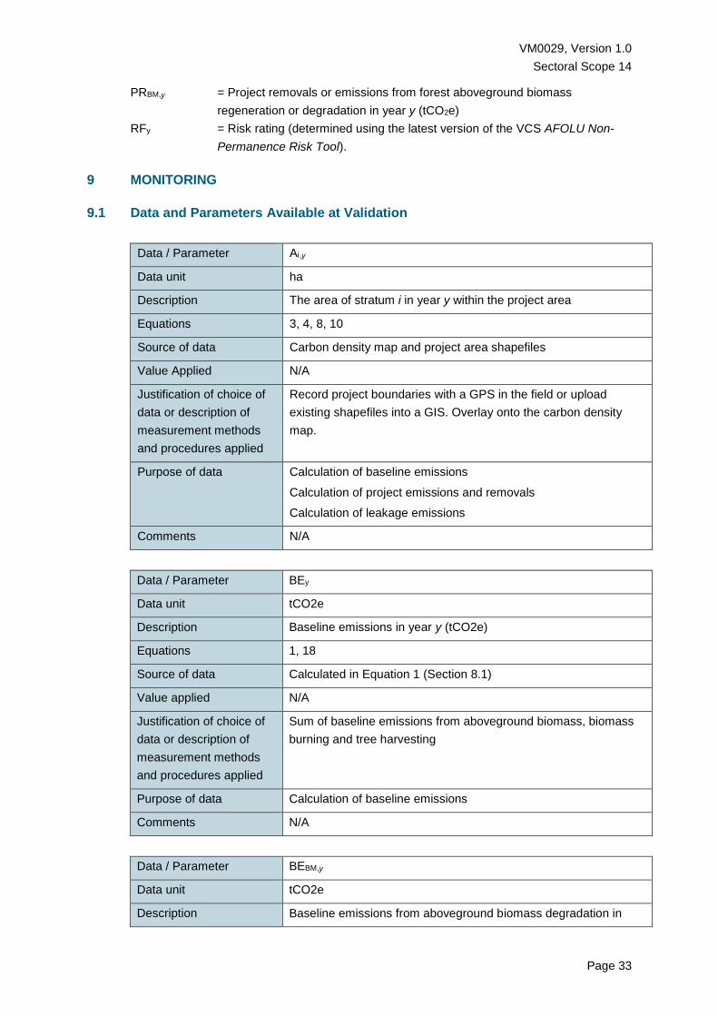
VM0029, Version 1.0

Sectoral Scope 14

PRBM,y = Project removals or emissions from forest aboveground biomass

regeneration or degradation in year y (tCO2e)

RFy = Risk rating (determined using the latest version of the VCS AFOLU Non-

Permanence Risk Tool).

9 MONITORING

9.1 Data and Parameters Available at Validation

Data / Parameter Ai,y

Data unit ha

Description The area of stratum i in year y within the project area

Equations 3, 4, 8, 10

Source of data Carbon density map and project area shapefiles

Value Applied N/A

Justification of choice of

data or description of

measurement methods

and procedures applied

Record project boundaries with a GPS in the field or upload

existing shapefiles into a GIS. Overlay onto the carbon density

map.

Purpose of data Calculation of baseline emissions

Calculation of project emissions and removals

Calculation of leakage emissions

Comments N/A

Data / Parameter BEy

Data unit tCO2e

Description Baseline emissions in year y (tCO2e)

Equations 1, 18

Source of data Calculated in Equation 1 (Section 8.1)

Value applied N/A



measurement methods


Sum of baseline emissions from aboveground biomass, biomass

burning and tree harvesting


Comments N/A

Data / Parameter BEBM,y

Data unit tCO2e

Description Baseline emissions from aboveground biomass degradation in

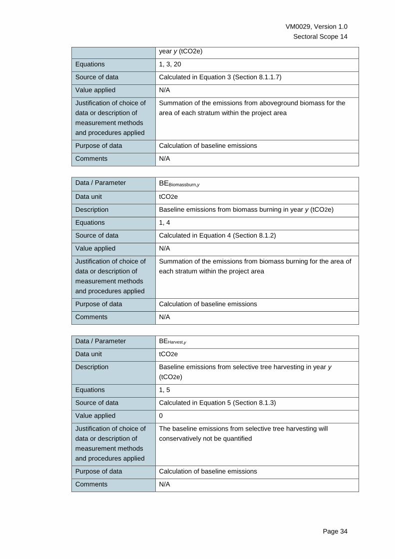
VM0029, Version 1.0

Sectoral Scope 14

year y (tCO2e)

Equations 1, 3, 20

Source of data Calculated in Equation 3 (Section 8.1.1.7)

Value applied N/A



measurement methods


Summation of the emissions from aboveground biomass for the

area of each stratum within the project area


Comments N/A

Data / Parameter BEBiomassburn,y

Data unit tCO2e

Description Baseline emissions from biomass burning in year y (tCO2e)

Equations 1, 4

Source of data Calculated in Equation 4 (Section 8.1.2)

Value applied N/A



measurement methods


Summation of the emissions from biomass burning for the area of

each stratum within the project area


Comments N/A

Data / Parameter BEHarvest,y

Data unit tCO2e

Description Baseline emissions from selective tree harvesting in year y

(tCO2e)

Equations 1, 5

Source of data Calculated in Equation 5 (Section 8.1.3)

Value applied 0



measurement methods


The baseline emissions from selective tree harvesting will

conservatively not be quantified


Comments N/A

VM0029, Version 1.0

Sectoral Scope 14

Data / Parameter BLPROBEarlyburn,i

Data unit tCO2e

Description Baseline early burning probability occurring in stratum i (fraction)

Equations 2


Value applied N/A



measurement methods


Baseline relative probability of early burning per stratum, as a

GapFire model input value


Comments N/A

Data / Parameter BLPROBLateburn,i

Data unit tCO2e

Description Baseline late burning probability occurring in stratum i (fraction)

Equations 2


Value applied N/A



measurement methods





Comments N/A

Data / Parameter BLPROBNoburn,i

Data unit tCO2e

Description Baseline No Burning Probability occurring in stratum i (fraction)

Equations 2


Value applied N/A



measurement methods





Comments N/A

VM0029, Version 1.0

Sectoral Scope 14

Data / Parameter Earliest possible burn date

Data unit Day/Month

Description The first day of the early burning season.

Equations N/A

Source of data Default date, expert opinion

Value applied Either the day at the beginning of the dry season at which the

monthly running average rainfall (at least 5 years of data) first falls

below 33 percent of peak wet season rainfall; or another locally-

appropriate date supported by credible expert opinion.



measurement methods


At research site Kilwa, the 33 percent of peak rainfall thresholds

coincide with the dates generally used for the start and end of the

dry season, as well as with first detection of fires at the start of the

dry season (around Day of Year 125, see Fig. 12 in Annex 1).

A monthly (28 day) running average is appropriate to smooth out

spikes from only a few years’ worth of data. The average must be

computed from the 14 days running up to and including the date

concerned, and the 14 days that follow it.

Due to the recent rains, only a few fires can expect to burn close

to this date, and thus allowing local flexibility in its determination

should not have a significant impact on emission reductions.


Comments N/A

Data / Parameter Early burning season cut-off date

Data unit Day and month

Description The last day of the early burning season. The cut-off date is

chosen and fixed at project validation for the duration of the

crediting period.

Equations N/A

Source of data Default date, expert opinion

Value applied Default date is the 30th day of June (day 181 of the year or 182 in

leap years), but expert opinion may establish a project-specific

cut-off date as an alternative.



measurement methods


Project-specific cut-off dates should approximate the average date

on which conditions allow fires to burn through the night.

On the one hand, it is important that the date is not set too late,

which could increase the risk that the project’s fire management

activities close to the cut-off date cause unintentional damage. On

the other hand, it should not be set too early as this will give the

project too small a window to carry out its fire management

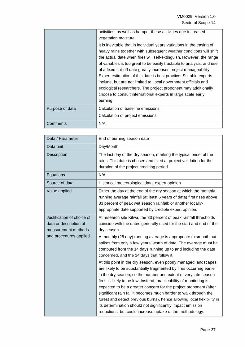
VM0029, Version 1.0

Sectoral Scope 14

activities, as well as hamper these activities due increased

vegetation moisture.

It is inevitable that in individual years variations in the easing of

heavy rains together with subsequent weather conditions will shift

the actual date when fires will self-extinguish. However, the range

of variables is too great to be easily tractable to analysis, and use

of a fixed cut-off date greatly increases project manageability.

Expert estimation of this date is best practice. Suitable experts

include, but are not limited to, local government officials and

ecological researchers. The project proponent may additionally

choose to consult international experts in large scale early

burning.


Calculation of project emissions

Comments N/A

Data / Parameter End of burning season date

Data unit Day/Month

Description The last day of the dry season, marking the typical onset of the

rains. This date is chosen and fixed at project validation for the

duration of the project crediting period.

Equations N/A

Source of data Historical meteorological data, expert opinion

Value applied Either the day at the end of the dry season at which the monthly

running average rainfall (at least 5 years of data) first rises above

33 percent of peak wet season rainfall; or another locally-

appropriate date supported by credible expert opinion.



measurement methods


At research site Kilwa, the 33 percent of peak rainfall thresholds

coincide with the dates generally used for the start and end of the

dry season.

A monthly (28 day) running average is appropriate to smooth out

spikes from only a few years’ worth of data. The average must be

computed from the 14 days running up to and including the date

concerned, and the 14 days that follow it.

At this point in the dry season, even poorly managed landscapes

are likely to be substantially fragmented by fires occurring earlier

in the dry season, so the number and extent of very late season

fires is likely to be low. Instead, practicability of monitoring is

expected to be a greater concern for the project proponent (after

significant rain fall it becomes much harder to walk through the

forest and detect previous burns), hence allowing local flexibility in

its determination should not significantly impact emission

reductions, but could increase uptake of the methodology.

VM0029, Version 1.0

Sectoral Scope 14



Comments N/A

Data / Parameter CountPixi,y

Data unit Count (integer value)

Description Number of countable pixels in stratum i in year y. Observations are

invalid when they are inconclusive due to cloud cover or missing

data.

Equations 2

Source of data Composite map of satellite images (eg, Landsat or SPOT)

Value applied N/A



measurement methods


The composite map is made by compiling as many images as

possible for the 10-year period of analysis and applying a burned

areas detection algorithm (eg, by applying the spectral index

method as described in Bastarrika et al, 2013).


Comments N/A

Data / Parameter CountEarlyburni,y


Description Number of countable pixels in stratum i in year y that showed

burning in the early burning season.

Equations 2


Value applied N/A



measurement methods







Comments N/A

Data / Parameter CountLateburni,y


Description Number of countable pixels in stratum i in year y that showed

burning in the late burning season.

Equations 2

VM0029, Version 1.0

Sectoral Scope 14


Value applied N/A



measurement methods







Comments N/A

Data / Parameter CountNoburni,y


Description Number of countable pixels in stratum i in year y that showed no

burning in both the early and the late burning season.

Equations 2


Value applied N/A



measurement methods







Comments N/A

Data / Parameter BBMCi,sy

Data unit tC/ha

Description Carbon stored in aboveground biomass per hectare in stratum i in

GapFire simulation year y in the baseline scenario

Equations 3, 17

Source of data GapFire model output

Value applied N/A



measurement methods


The GapFire model simulates the biomass response of an

ensemble of tree-sized forest patches to different fire regimes,

input as probabilities of early burn, late burn and no burn, for both

the baseline and the project scenarios. A simulation is run for each

stratum, which is specified by inputting the median carbon density

of the stratum. The output is the simulated carbon stock changes

over time.



VM0029, Version 1.0

Sectoral Scope 14

Comments N/A

Data / Parameter AvCMortBLi,y

Data unit tC/ha

Description Average yearly carbon stored in biomass dying as a result of tree

mortality over the first 10 years’ output of the yearly GapFire

model baseline simulation for stratum i in year y (see Section

8.1.1.7)

Equations 4


Value applied N/A



measurement methods


The GapFire model simulates the biomass response, including

mortality (both background and fire-induced) of an ensemble of

tree-sized forest patches to different fire regimes. Annual carbon

losses are available as a GapFire output.


Comments N/A

Data / Parameter Gg

Data unit kg t-1 dry matter burnt

Description Emission factor for gas g

Equations 4, 10

Source of data Section III and annex 2 of VCS module VMD0013, Estimation of

greenhouse gas emissions from biomass burning (E-BB).

Value applied Use values for ‘Tropical forest’



measurement methods


Miombo woodland is a type of tropical forest. The values for

‘Savannah and grassland’ relate to the burning of grasses.

Purpose of data Calculation of baseline and project emissions from biomass

burning

Comments

Data / Parameter GWPg

Data unit t CO2/t gas g

Description Global warming potential for gas g

Equations 4, 10

Source of data Default values from IPCC SAR

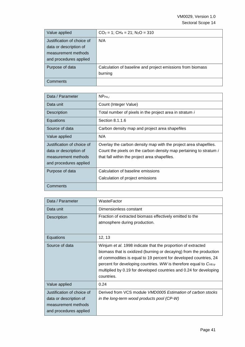
VM0029, Version 1.0

Sectoral Scope 14

Value applied CO2 = 1; CH4 = 21; N2O = 310



measurement methods


N/A

Purpose of data Calculation of baseline and project emissions from biomass

burning

Comments

Data / Parameter NPPA,i

Data unit Count (Integer Value)

Description Total number of pixels in the project area in stratum i

Equations Section 8.1.1.6


Value applied N/A



measurement methods


Overlay the carbon density map with the project area shapefiles.

Count the pixels on the carbon density map pertaining to stratum i

that fall within the project area shapefiles.



Comments

Data / Parameter WasteFactor

Data unit Dimensionless constant

Description Fraction of extracted biomass effectively emitted to the

atmosphere during production.

Equations 12, 13

Source of data Winjum et al. 1998 indicate that the proportion of extracted

biomass that is oxidized (burning or decaying) from the production

of commodities is equal to 19 percent for developed countries, 24

percent for developing countries. WW is therefore equal to CXB,ty

multiplied by 0.19 for developed countries and 0.24 for developing

countries.

Value applied 0.24



measurement methods


Derived from VCS module VMD0005 Estimation of carbon stocks

in the long-term wood products pool (CP-W)

VM0029, Version 1.0

Sectoral Scope 14

Purpose of data Calculation of project emissions

Comments N/A

Data / Parameter BEF

Data unit Dimensionless constant

Description Biomass expansion factor.

Equations 12, 13

Source of data The source of data must be chosen with priority from higher to

lower preference as follows:

(a) Existing local forest type-specific;

(b) National forest type-specific or eco-region-specific (eg from

national GHG inventory);

(c) Forest type-specific or eco-region-specific from neighboring

countries with similar conditions.

(d) Global forest type or eco-region-specific (eg, IPCC 2006

Inventory Guidelines, AFOLU, Chapter 4, Table 4.5)

Value applied Variable



measurement methods


N/A


Comments N/A

Data / Parameter CF

Data unit tC/tDry Matter

Description Carbon fraction of woody biomass

Equations 4, 10, 12, 13, 14, 15

Source of data IPCC 2006, AFOLU, Chapter 4, Table 4.3

Value applied 0.47



measurement methods


The IPCC is considered a widely acceptable source of default

values.



Comments N/A

VM0029, Version 1.0

Sectoral Scope 14

9.2 Data and Parameters Monitored

Data / Parameter Aboveground tree biomass

Data unit tC/ha

Description Aboveground tree biomass is determined in sample plots for the

purpose of validation of the carbon density map

Equations N/A

Source of data Field measurements

Description of

measurement methods

and procedures to be

applied

Measurements must be taken in sample plots, each not smaller

than 0.5 ha in size, and should be distributed across the

landscape in an unbiased manner. Aboveground tree biomass

with diameter >5 cm must be measured using scientific best

practice, must comply with VCS requirements for accuracy and

precision and must be calculated using an allometric equation that

is 1) published in peer-reviewed scientific literature and 2)

justifiably appropriate for the ecological conditions in the project

area. If alternative field data is used, justification must be provided

to show how it is equivalent to or exceeds these requirements.

Frequency of

monitoring/recording

When the carbon density map is first made and every time it is

revised

QA/QC procedures to be

applied

Scientific common practice must be used to check for implausible

data entries (eg, identification and elimination, correction or re-

measurement of outliers).

At least 5 percent of trees must be re-measured and data

compared (re-measurement may have taken place at an earlier or

later date, so long as both measurements are available when the

carbon density map is made). The average plot-scale

measurement plausibility rate (after allowing for expected tree

growth) must be at least 85%. Where the mean measurement

plausibility rate is less than 90% in one or more plots these plots

should be included in subsequent analysis if it is conservative to

do so (ie, lower growth is detected) and excluded where they

would lead to greater carbon gains being detected.



Comments N/A

Data / Parameter Ai,y

Data unit ha

Description The area of stratum i in year y within the project area

Equations 3, 4, 8, 10

VM0029, Version 1.0

Sectoral Scope 14


Description of

measurement methods


applied

Record project boundaries with a GPS in the field or upload

existing shapefiles into a GIS. Overlay onto the carbon density

map.

Frequency of


Every time the project area and the carbon density map are

revised


applied

Actions by the operator must be double-checked and signed off by

a supervisor for correctness




Comments N/A

Data / Parameter Areaz ,y

Data unit ha

Description The area of FMU z in year y within the project area

Equations 7

Source of data Project area shapefiles

Description of

measurement methods


applied

Record FMU boundaries with a GPS in the field or upload existing

shapefiles into a GIS

Frequency of


Every time the project area is revised


applied

Actions by the operator must be double-checked and signed off by

a supervisor for correctness


Comments N/A

Data / Parameter FFEarlyBurn,z,y

Data unit Fraction (dimensionless)

Description Early burning fire frequency in FMU z in year y

Equations 7

Source of data Field observations

Description of

measurement methods


applied

See Section 9.3.2

VM0029, Version 1.0

Sectoral Scope 14

Frequency of


First monitoring event of each year


applied

Geo-located digital photos must be taken at each checkpoint, and

a random selection of at least 5 percent must be checked

afterwards for accuracy (burn / no-burn).


Comments N/A

Data / Parameter FFLateBurn,z,y


Description Late burning fire frequency in FMU z in year y

Equations 7


Description of

measurement methods


applied

See Section 9.3.2

Frequency of


Second monitoring event of each year


applied





Comments N/A

Data / Parameter FFNoBurn,z,y


Description No burning fire frequency in FMU z in year y

Equations 7


Description of

measurement methods


applied

See Section 9.3.2

Frequency of


Second monitoring event of each year


applied




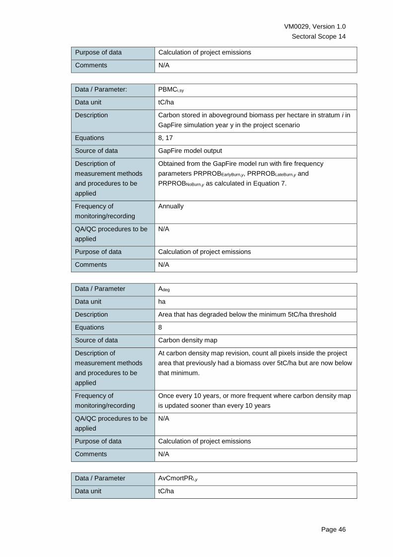
VM0029, Version 1.0

Sectoral Scope 14


Comments N/A

Data / Parameter: PBMCi,sy

Data unit tC/ha

Description Carbon stored in aboveground biomass per hectare in stratum i in

GapFire simulation year y in the project scenario

Equations 8, 17


Description of

measurement methods


applied

Obtained from the GapFire model run with fire frequency

parameters PRPROBEarlyBurn,y, PRPROBLateBurn,y and

PRPROBNoBurn,y as calculated in Equation 7.

Frequency of


Annually


applied

N/A


Comments N/A

Data / Parameter Adeg

Data unit ha

Description Area that has degraded below the minimum 5tC/ha threshold

Equations 8

Source of data Carbon density map

Description of

measurement methods


applied

At carbon density map revision, count all pixels inside the project

area that previously had a biomass over 5tC/ha but are now below

that minimum.

Frequency of


Once every 10 years, or more frequent where carbon density map

is updated sooner than every 10 years


applied

N/A


Comments N/A

Data / Parameter AvCmortPRi,y

Data unit tC/ha

VM0029, Version 1.0

Sectoral Scope 14

Description Average annual carbon stored in biomass dying as a result of tree

mortality over the first 10 years’ output of the annual GapFire

model project simulation for stratum i (see Section 8.1.1.7)

Equations 10


Description of

measurement methods


applied

Obtained from the GapFire model run with fire frequency

parameters PRPROBEarlyBurn,y, PRPROBLateBurn,y and

PRPROBNoBurn,y as calculated in Equation 7.

Frequency of


Annually


applied

N/A


Comments N/A

Data / Parameter Areg,y

Data unit ha

Description Areas that previously degraded below the 5 tC/ha threshold, but

that in year y regenerate above this threshold

Equations 8

Source of data Carbon density map

Description of

measurement methods


applied

At carbon density map revision, count all pixels inside the project

area that had once been over the 5tC/ha threshold, then on a

previous revision had been found to have degraded below the

5tC/ha biomass threshold, but have since regenerated such that

biomass is once again over 5tC/ha.

Frequency of


Once every 10 years, or more frequent where carbon density map

is updated sooner than every 10 years


applied

N/A


Comments N/A

Data / Parameter HVj,y

Data unit m3

Description Harvested bole volume of species j in the project area in year y

Equations 11

Source of data Field measurements and volume calculations

VM0029, Version 1.0

Sectoral Scope 14

Description of

measurement methods


applied

Of each harvested tree, record the species.

Take diameter measurements at the base and the top of the bole

and calculate the average diameter (Daverage).

Measure the length (l) of the bole.

HVj,y =(Daverage / 2)2 × π × l

Frequency of


Each time a tree is harvested


applied

At least 5 percent of trees must be re-measured and data

compared


Comments N/A

Data / Parameter Dt,j,y

Data unit cm

Description Diameter at Breast Height of harvested tree t of species j in year y

Equations 13

Source of data Field measurements

Description of

measurement methods


applied

Diameter measured at Breast Height before the tree is harvested

using a measuring tape

Frequency of


Each time a tree is harvested


applied

At least 5 percent of log measurements (randomly chosen) should

be checked against recorded tree diameter for consistency. Since

log volume is the basis for sale price, Forest Managers are

incentivized to maximize log diameter, and thus one can be

confident that data is not biased on the low side (ie, is

conservative with respect to emissions reductions achieved after

deducting project emissions and removals).

Purpose of data Calculation of project emissions and removals

Comments N/A

Data / Parameter WDj

Data unit t dry matter /m3

Description Wood density of harvested species j

Equations 12, 13, 14

Source of data Field measurements or available literature

Description of Where literature sources can be found for WDj, the project

VM0029, Version 1.0

Sectoral Scope 14

measurement methods


applied

proponent may choose to use the published values or establish

their own values (see below). The source of literature-derived data

must be chosen with priority from higher to lower preference as

follows:

(a) National species-specific or group of species-specific (eg, from

national GHG inventory);

(b) Species-specific or group of species-specific from neighboring

countries with similar conditions.

(c) Global species-specific or group of species-specific (eg, IPCC

2006 INV GLs, AFOLU, Chapter 4, Tables 4.13 and 4.14).

Species-specific wood densities may not always be available, and

may be difficult to apply with certainty in the typically species rich

forests of the tropics. Therefore, it is acceptable practice to use

wood densities developed for forest types or plant families or

species groups.

Where literature sources cannot be found for species-specific

WDj, the project proponent must establish WDj of harvested

species j as recorded upon harvesting by the water displacement

method, as follows:

1) Take a piece of wood from the middle of the harvested

bole.

2) Oven-dry the piece of wood using standard procedures to

achieve wood moisture content below 15 percent.

3) Establish weight (W) of the dry piece of wood.

4) Put water in a container that allows for accurate water

volume measurement. Measure the volume (V1) of water

in the container.

5) Submerge the dry piece of wood fully in the water.

Measure the volume of water (V2) in the container again.

6) The volume of the piece of wood is V = V2 – V1

7) WDj = W / V

8) Convert the measurement units to t / m3

Frequency of


Once, when the first tree of species j is harvested


applied

Repeat measurement of WDj several times to establish an

average value within the 90 percent confidence interval.


Comments N/A

Data / Parameter VMT,j,y

Data unit m3

Description Volume of species j in year y that enters the medium-term wood

VM0029, Version 1.0

Sectoral Scope 14

products pool (remaining in this pool between 3 and 100 years)

Equations 15

Source of data Timber sales records, interviews with timber buyers and

processors, expert opinion and credible sources

Description of

measurement methods


applied

Of each harvested tree species record the most likely end uses

and determine their relative proportions of the harvested volume.

Include the volume that goes into end uses with a life-time

between 3 and 100 years into VMT,j,y

Frequency of


Each time any volume of species j is processed and/or sold


applied

Contact details of interviewees must be stored so that likely end

uses and their relative proportions can be independently verified.


Comments N/A

Data / Parameter FSm,fc

Data unit %

Description Proportion of fires started by fire cause fc in month m, weighted by

area affected.

Equations Matrix computation of leakage emissions

Source of data Interviews, rural appraisals and other local expert knowledge.

Description of

measurement methods


applied

The proportions of all identified fire causes fc must sum to 100

percent for each month.

Frequency of


Annually


applied

N/A

Purpose of data Calculation of leakage emissions

Comments N/A

Data / Parameter Dfc

Data unit %

Description Rate of fire displaceability of fire cause fc

Equations Matrix computation of leakage emissions

Source of data Interviews, rural appraisals and other local expert knowledge.

Description of

measurement methods

The rates are not expected to vary by month or year

VM0029, Version 1.0

Sectoral Scope 14


applied

Frequency of


Annually


applied

N/A

Purpose of data Calculation of leakage emissions

Comments N/A

9.3 Description of the Monitoring Plan

9.3.1 Carbon Density Map Validation

The carbon density map must be ground-truthed using field data appropriate for this purpose.

Data must be collected from sample plots that can be easily related to pixels in the remotely

sensed data. Sample plots should therefore be located using some basic stratification to

ensure broad coverage of the range of forest densities. Sufficient sample plots must be

surveyed to bootstrap the classification function, and others to assess uncertainty whilst

generating a narrow enough confidence limit that meets the requirements of Section 8.1.1.1.

Due to the heterogeneity in miombo vegetation cover, main sample plots must cover at least

0.5ha. However, the survey design may incorporate smaller sub-plots in which a greater

range of information is collected (eg, on smaller stem sizes), and which can be used to

improve the classification of remotely sensed data. The size of the largest plot in each cluster

must be larger than the desired map resolution (at least twice as large in each direction).

Aboveground biomass in trees with DBH >5cm, and stem density for saplings 1-5cm DBH,

must be measured using scientific best practice and must comply with VCS requirements for

accuracy and precision. Biomass values must be calculated using an allometric equation that

is 1) published in peer-reviewed scientific literature and 2) justifiably appropriate for the

ecological conditions in the project area.16

9.3.2 Annual Monitoring of Fire Frequencies

Monitoring the project scenario must be undertaken by direct field observations, since

estimates derived from remote sensing data generally have too wide an error margin for

specific project sites.

Due to the unpredictability of fire spread, each forest management unit (FMU) must be

separately monitored.

16 Note that the GapFire model itself uses the tree allometry derived by Ryan et al. (2011) from N’Hambita in

Mozambique. Substituting alternative allometries in the GapFire model is only feasible if they include leaf area

(which many do not). However, using different allometries in the carbon density map computation and GapFire

model is not a fundamental problem, and of less importance than using the most appropriate allometric

relationship in validating the carbon density map.

VM0029, Version 1.0

Sectoral Scope 14

Monitoring must take place twice a year, at the end of the early burning season, and at the

end of the late burning season. Monitoring must take place within one calendar month either

side of the early burning season cut-off date and end of burning season date, respectively. If

either monitoring requirement is missed or incomplete, then no emissions reductions may be

claimed for that FMU that year, and for future years the baseline fire regime should be

assumed to have taken place. Where monitoring is complete for some but not all FMUs, only

the monitored FMUs may claim emission reductions. FMUs where monitoring is not

completed two years’ running must be visually assessed for deforestation or significant

disturbance at the end of the second year since the project start date in the FMU, or since the

previous monitoring event, whichever is later. Failure to do so will lead to the automatic

assumption that all aboveground carbon stocks in the area have been emitted. The loss event

must be reported to VCS in accordance with VCS requirements. The same occurs if the visual

assessment detects deforestation or significant disturbance.

Monitoring fire frequency must be undertaken using a set of checkpoints distributed

throughout the forest in the FMU. The surveyor must assess the ground immediately beneath

their feet at each checkpoint. The surveyor records a fire if some or all of that small patch of

ground has blackened due to passage of fire. If no such signs are evident, then no fire is

detected. The fire frequency is then specified as the percentage of checkpoints at which a fire

was recorded (the detection rate).

In the case of the early burning season monitoring period, all fires are assumed to be new

fires, and no adjustments are required. In the case of the late burning season monitoring

period, the fire frequency is defined as the difference between the two percentages:

FFlate season only = FFlate season detection rate – FFearly season detection rate (21)

Note that the monitoring of burn probabilities does not consider carbon density strata, as

explained in Section 8.2.1.1.

9.3.2.1 Distribution of Fire Monitoring Checkpoints

At least 86 checkpoints are required across the entire project area so as to ensure the 95

percent confidence interval is no wider than 15 percent17. In practice it is recommended at

least 100 checkpoints be surveyed in each FMU each monitoring period, as a cost-effective

way to minimize errors being passed through to the model. These checkpoints may be either

permanently established or newly generated in each monitoring period, or some middle option

(eg, checkpoints may be unmarked but on permanent transects, such that roughly the same

set of points is monitored each year). The project proponent who chooses to use permanent

or semi-permanently located checkpoints must justify this choice, and show how they are not

subject to a biased or unrepresentative fire management or other treatment compared to the

rest of the FMU.

17 From the binomial distribution, assuming that the probability of a burn is not close to 0 or 1, the

minimum is 43 for a single monitoring exercise. Since FFlateseasononly depends on two monitoring

exercises then 86 checkpoints is a conservative minimum to ensure the confidence interval is no

wider than 15 percent.

VM0029, Version 1.0

Sectoral Scope 14

Checkpoints may be located either through a purely random process, or through a partly

random process which takes into account logistical constraints to some degree. Where the

process is not fully random, the project proponent must clearly describe the steps taken to

avoid accidental bias (eg, transect or plot locations should be generated without reference to

biophysical data beyond the minimum required for the process (such as FMU boundaries)).

Except in the case where a new set of checkpoints is generated directly and purely randomly

each monitoring period, checkpoints and their spatial underpinning (eg, transect lines) should

be evenly distributed throughout the forest. Checkpoint location should also not be biased

with respect to biomass or to other relevant variables such as altitude and steepness of slope

(which affect fire spread). The project description must set out specific procedures and criteria

for ensuring that this criterion is met. Where a random checkpoint generation process fails

these tests, the project proponent may either add additional checkpoints, or move existing

ones so as to come within the representativeness criteria (so long as the process to do so is

itself clearly random and not informed by detailed knowledge of the FMU).

In defining such procedures, it is important to note the GapFire model produces estimates of

emissions reductions that scale roughly linearly with starting biomass. In this situation it is not

necessary to ensure minimum representation from each stratum, so long as the distribution of

biomass at checkpoints is statistically similar to the FMU population in both mean and

variance.

9.3.2.2 Checking for Forest Loss

The baseline carbon density map must be revised at least every 10 years (see section 9.3.3

below), but catastrophic fires and other forest loss events from unplanned land use change

could happen at any time. If the twice-yearly monitoring of fire frequencies detects such

occurrences, then the area of any affected area must be recorded in the field with a GPS. The

area of each carbon density stratum present in the affected area must be determined from the

carbon density map. It will be assumed that all aboveground carbon stocks in the area will

have been emitted. The loss event must be reported to VCS in a timely manner. The project

proponent may complement this with additional monitoring that may be less regular or

rigorous in design.

9.3.3 Revision of Carbon Density Map

This methodology requires a biomass carbon density map that is never more than 10 years

old. Thus, the map must be updated at least every 10 years, though the project proponent

may choose to update more frequently if they so wish.

To update the carbon density map, the same procedures as given in sections 8.1.1.1 to

8.1.1.3 above must be followed.

During revision of the carbon density map, project areas that are identified as having

degraded below the lower threshold value in the project scenario must be excluded from

subsequent modeling of carbon fluxes (ie, no further claims may be made on those areas). It

must be assumed that all aboveground tree carbon density is emitted instantly (Equation 8,

Section 8.2.1.1). In a subsequent revision of the carbon density map, where such excluded

VM0029, Version 1.0

Sectoral Scope 14

areas are determined to have regenerated again above the 5 tC/ha threshold, they may be re-

included in the modeling of carbon fluxes, at which point their aboveground tree carbon

density is treated as an instantaneous sequestration and is added to the project’s emission

reductions (Equation 8).

For project areas that regenerate above the higher threshold value in the project scenario

during the project crediting period, these specific areas may remain within the project. Eligible

areas must be identified as pixels on a carbon density map as per Section 8.1.1.1.

Before stratifying and using the new carbon density map, the new values must be compared

to predicted model output in the Project Area. To do this, the revised carbon density map

must be overlaid with the existing project area. Then, calculate the following for the project

area:

TPBC = Total Predicted aboveground Biomass Carbon (tonnes) derived from

GapFire model predictions to date

TABC = Total Actual aboveground Biomass Carbon (tonnes) derived from the revised

carbon density map

λTABC = 95 percent upper confidence limit of TABC

Comparing these figures leads to one of three possible outcomes:

TABC > TPBC

The total new biomass in the Project Area is greater than the total biomass predicted

by the GapFire model. In this case the model predictions were conservative. No

action is required, and the new carbon density map may be adopted.

TABC ≤ TPBC ≤ λTABC

The total biomass predicted by the GapFire model is within the margin of error on the

carbon density map. No action is required, and the new carbon density map may be

adopted.

TPBC > λTABC

The new total biomass is substantially less than predicted, and outside the margin of

error. The project must account for the loss.

In the third case, the project must register a loss event in the year that the new carbon density

map was constructed as per Equation 22.

Emissions Detected at Map Update, EDMU = (TABC – TPBC) × 44/12 (22)

If EDMU is less than the total claim of avoided emissions, NERRy, as calculated in step 8.4,

then deduct EDMU from the total. If EDMU exceeds NERRy, report the loss event in

accordance with VCS requirements.

All deviations from the model should be reported to the University of Edinburgh so that they

can be incorporated into model revisions.

VM0029, Version 1.0

Sectoral Scope 14

Stratify the new carbon density map as per Section 8.1.1.2, and use the map as the basis for

GapFire model predictions for the following 10 years (ie, these are likely to differ from the

previous strata).

Areas of the map that were previously above the minimum carbon density allowable in the

methodology, but have since dropped below it, must be excluded from future crediting (as per

Section 5.2). However, where it cannot be demonstrated from monitoring that the cause of the

reduction in carbon density was a land use change event or a catastrophic event, such areas

must still be included in the analysis of the next carbon density map update and the

calculation of EDMU. Where, at that point, the biomass has risen above the minimum

biomass allowable in the methodology, such areas may once again be incorporated into the

project for crediting of emissions reductions.

Areas of the map that were previously below the maximum biomass allowable in the

methodology, but have since risen above that threshold may remain, since although future fire

frequencies may be assumed to be much lower, even without sustained fire management, all

future gains made are the result of previous project action, and thus claimable. Additional

strata should be added to those listed in Section 8.1.1.2, Table 4, at 5 ton intervals to account

for such increases.

9.3.4 Decadal Revision of Fire History Baseline

Revalidate the baseline every 10 years using one of the following options:

1) Provide a qualitative justification showing how local fire practices have not changed

significantly (eg, frequency of burning, and late season fires in particular have not

significantly decreased). A decline in early season fires is allowable so long as it is

offset by an equal or larger increase in late season fires. This justification must be

supported with credible evidence and by local experts. Where there is reason to

believe that local fire practices might have improved so as to reduce the severity of

the baseline scenario, this option for revising the fire history is not permitted.

2) Redo the fire history derived from burn scar identification on satellite images as

specified in Section 8.1.1.5. Due to the project activities implemented over the

previous 10 years, this may involve determination of a new BRR that excludes both

project areas, and other areas that could be protected from burning by project

activities (ie, a “fire shadow” effect in which project areas block fire routes, thus

reducing fire frequency in areas downwind of the prevailing wind direction). This new

BRR must satisfy all the relevant criteria listed in Section 8.1.1.3, and must be

covered in the biomass map.

Note that it is not necessary to update the biomass map and the fire history baseline at the

same time. However, if the BRR has been expanded, this may necessitate a larger biomass

map.

VM0029, Version 1.0

Sectoral Scope 14

10 REFERENCES

Archibald, S., Lehmann, C. E., Gómez-Dans, J. L., and Bradstock, R. A. 2013. Defining

pyromes and global syndromes of fire regimes. Proceedings of the National Academy of

Sciences, 110(16), 6442-6447.

Bastarrika, A., Chuvieco, E., and Martín. M.P. 2013 "Mapping burned areas from Landsat

TM/ETM+ data with a two-phase algorithm: Balancing omission and commission errors."

Remote Sensing of Environment 115.4: 1003-1012.

http://www.ehu.es/aitor.bastarrika/AitorDocs/Bastarrika_2011a.pdf

Bridges, E.M. 1990. World Geomorphology. Cambridge University Press, UK.

ESA Climate Change Initiative, 2011: Fire, User requirements document, http://www.esa-fire-

cci.org/webfm_send/264

Frost. P. 1996. The ecology of Miombo woodlands. In: B. Campbell (ed) The Miombo in

Transition: Woodlands and Welfare in Africa. CFIOR, Bogor.

Giglio, L., Loboda, T., Roy, D.P., Quayle, B. and Justice, C.O. 2009. An active-fire based

burned area mapping algorithm for the MODIS sensor. Remote Sensing of Environment 113:

408–420

GOFC-GOLD 2012, A sourcebook of methods and procedures for monitoring and reporting

anthropogenic greenhouse gas emissions and removals associated with deforestation, gains

and losses of carbon stocks in forests remaining forests, and forestation. GOFC-GOLD

Report version COP18-1, (GOFC-GOLD Land Cover Project Office, Wageningen University,

The Netherlands).

Hauf, H. 2012. Mitigating forest fires in Kilwa District, Tanzania: An investigation of

anthropogenic drivers. Student dissertation, University of Oxford Department of Continuing

Education. 49 pp.

IPCC. 2006, 2006 IPCC Guidelines for National Greenhouse Gas Inventories, Volume 4:

Agriculture, Forestry, and Other Land Use. Prepared by the National Greenhouse Gas

Inventories Programme, Eggleston H.S., Buendia L., Miwa K., Ngara T. and Tanabe K. (eds).

Published: IGES, Japan. http://www.ipcc-nggip.iges.or.jp/public/2006gl/index.html

Isango, J.A., 2007. Stand Structure and Tree Species Composition of Tanzania Miombo

Woodlands: A Case Study from Miombo Woodlands of Community Based Forest

Management in Iringa District. Working Papers of the Finnish Forest Research Institute 50:

43–56

Stronach, N. 2009. A review of the impact of fire on the carbon content, dynamics and

biodiversity value of miombo woodlands. Report for Fauna & Flora International.

Werger, M.J.A. and B.J. Coetzee. 1978. The Sudano-Zambezian Region. M.J.A. Werger,

editor. Biogeography and Ecology of Southern Africa. W. Junk, The Hague.

http://www.esa-fire-cci.org/webfm_send/264

http://www.esa-fire-cci.org/webfm_send/264

VM0029, Version 1.0

Sectoral Scope 14

White, F. 1983. The vegetation of Africa, a descriptive memoir to accompany the

UNESCO/AETFAT/UNSO Vegetation Map of Africa (3 Plates, Northwestern Africa,

Northeastern Africa, and Southern Africa, 1:5,000,000. UNESCO. Paris.

Winjum, J.K., Brown, S. and Schlamadinger, B. 1998. Forest harvests and wood products:

sources and sinks of atmospheric carbon dioxide. Forest Science 44: 272-284

VM0029, Version 1.0

Sectoral Scope 14

APPENDIX 1: THE GAPFIRE MODEL

This appendix was prepared by Sam Bowers and Prof. Mathew Williams of the University of

Edinburgh.

A1.1 Definitions

AGB

Aboveground biomass, the biomass of tree stems (incl. crowns)

Allometric equations

Tree allometry describes the quantitative relations between key, easy to measure characteristics of

trees and other more difficult to assess properties. Here we relate DBH to tree morphology.

Chronosequence

A series of forest sites with similar attributes that have been regrown following clearance and

abandonment, allowing the analysis of forest processes that occur over long time scales

ECMWF

European Centre for Medium Range Weather Forecasts, source of the ERA-interim global climate

reanalysis dataset

Fire intensity

A measure of the energy released by a fire, closely related to its expected impacts upon a woodland

ecosystem

FRI

Fire return interval, the mean time period between fires in years

GPP

Gross Primary Productivity, the rate at which organisms capture and store energy through

photosynthesis

MODIS

Moderate-Resolution Imaging Spectroradiometer, a NASA optical remote sensing instrument with a

data archive covering the period 1999-present

NDVI

Normalised Difference Vegetation Index, a measure of plant greenness calculated using

measurements of near infrared and red surface reflectance

Nhambita

Miombo woodland field site in central Mozambique

NPP

Net Primary Productivity, GPP minus the energy lost to respiration

PSP

Permanent sample plot, a woodland plot used to measure and monitor vegetation status

VM0029, Version 1.0

Sectoral Scope 14

Top-kill

Aboveground stem mortality, which is decoupled from rootstock mortality due to the importance of

resprouting in fire prone ecosystems

A1.2 Introduction

In order to understand the impacts of forest disturbance over long time periods, modelling techniques

may be used in place of direct measurements of difficult to detect forest degradation. A dynamic

model of forest biomass named GapFire has been developed to simulate the impacts of a variety of

fire regimes on the structure of miombo woodlands. The model forecasts the growth and mortality of

individual trees under future fire regimes based on an ensemble of tree-sized woodland patches.

When run under a range of fire return intervals (FRIs) and fire intensities, the model provides a

prediction of woodland response to an altered fire regime. Although a relatively simple model,

GapFire has been shown to be proficient at capturing the complex dynamics of miombo woodland

disturbance (Ryan and Williams, 2011).

This report provides a detailed description of how the model is structured and operated, including

discussion of principal assumptions made and their impact on model predictions. Throughout the

modelling process an emphasis has been placed on utilizing all available field data from miombo

woodlands. As data on the dynamics in some areas of miombo woodland growth, mortality and fire

are limited, the model ensures that predictions lead to conservative estimates of biomass changes in

place of a best-guess estimate of miombo woodland response.

A1.3 Model Overview

The death of trees in natural woodlands results in small ‘gaps’ opening in the tree canopy. These

openings in otherwise shaded forest allow for light to penetrate through the forest canopy, stimulating

the growth of small trees to re-populate the opening. By explicitly modelling the growth, mortality and

regeneration of trees at these forest gaps, the balance between carbon sequestration through forest

regrowth and carbon emission from woodland disturbance may be predicted as Figure 1). Gap

dynamics have been widely utilized by forest land managers for their close relation to many practical

forest applications. Gap models are particularly appropriate for describing miombo woodlands where

woodland structure is profoundly modified by frequent disturbance events. The model is similar in

conception to many other gap models (Shugart and Smith, 1996, Williams, 1996) that have been used

previously in miombo woodlands (Desanker, 1996, Desanker and Prentice, 1994) and also to

simulate the effects of fire (Miller and Urban, 2000). A gap-modelling approach has advantages from

its explicit representation of population structure and variability, its ability to explore the stochastic

nature of disturbance events through large modelling ensembles, and because it allows density-

dependent feedbacks on growth through light competition. The model presented here in a modified

arrangement of the published model of Ryan and Williams (2011) for the prediction of biomass

change.

VM0029, Version 1.0

Sectoral Scope 14

Figure 1: Diagrammatic Representation of Gapfire, Showing Patch Initialization, Growth in

Response to Photosynthetically Active Radiation (PAR), Fire Induced Mortality and

Regeneration

GapFire has been developed to model stems, their light environment, phenology, mortality and

resultant carbon fluxes as described in figure 2 below. The model simulates individual ‘patches’ with

an area roughly equivalent to the canopy of a large tree (0.02 ha). Light is intercepted by the leaves of

each stem at a rate relating to the height of leaves in the woodland canopy. Leaf area is calculated as

a function of stem diameter, and varies through the year with observations of leaf phenology,

restricting growth to the wet season when soil moisture is plentiful. Intercepted light is converted to

carbon using a miombo-specific light response curve. Assimilated carbon is allocated to respiration,

leaf and fine-root formation, with remaining carbon allocated to increasing stem and large root

biomass. As stems increase in biomass their morphology (DBH, leaf area, canopy structure) is altered

according to a series of allometric models developed for miombo woodlands (see 2.4 below).

Following annual growth, stems are exposed to a chance of top-kill from intrinsic sources or as a

result of fire, where probability of top-kill can be related to stem size, frequency and intensity of fire.

Each year woodland patches regenerate, with the resprouting of top-killed rootstocks and the

recruitment of new seedlings. As patches are small, and mortality and regeneration processes are

stochastic, the biomass change in a single patch will not represent the trends of miombo woodland as

a whole, hence the model is run as an ensemble of many patches, with mean trends representative of

the net change in miombo woodland carbon storage.

The following text gives a detailed overview of initialization, growth, mortality and regeneration in the

model. The model is summarized in a schematic diagram as described in figure 2 below.

PAR

Patch Initialisation Growth Mortality Regeneration

Next year

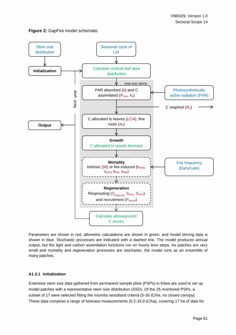
VM0029, Version 1.0

Sectoral Scope 14

Figure 2: GapFire model schematic

Parameters are shown in red, allometric calculations are shown in green, and model driving data is

shown in blue. Stochastic processes are indicated with a dashed line. The model produces annual

output, but the light and carbon assimilation functions run on hourly time steps. As patches are very

small and mortality and regeneration processes are stochastic, the model runs as an ensemble of

many patches.

A1.3.1 Initialization

Extensive stem size data gathered from permanent sample plots (PSPs) in Kilwa are used to set up

model patches with a representative stem size distribution (SSD). Of the 25 monitored PSPs, a

subset of 17 were selected fitting the miombo woodland criteria (5-35 tC/ha, no closed canopy).

These data comprise a range of biomass measurements (5.2-33.9 tC/ha), covering 17 ha of data for

Next y

ear

Initialization

Stem size

distribution

Calculate vertical leaf area

distribution

Seasonal cycle of

LAI

PAR absorbed (k) and C

assimilated (Pmax, kp)

Photosynthetically

active radiation (PAR)

C allocated to leaves (LCA), fine

roots (Afr)

Growth

C allocated to woody biomass

Mortality Intrinsic (Mi) or fire-induced (kearly,

λearly, klate, λlate)

Regeneration

Resprouting (Sresprout, Snew, Smort)

and recruitment (Precruit)

Fire frequency

(Early/Late)

Output

Calculate aboveground

C stocks

C respired (Ra)

loop over stems

VM0029, Version 1.0

Sectoral Scope 14

stem sizes 5-40 cm DBH and 170 ha of stems >40 cm DBH. The data were fitted with two exponential

trend lines, with a break point at 15 cm DBH to optimally fit observations of stem sizes as described in

Figure 3 below. From these trends, two probability density functions were generated from which stem

sizes may be randomly allocated to trees in model patches. A minimum stem size of 1 cm DBH was

imposed to match the size that a seedling may reach following one year of growth. An upper limit of

100 cm DBH was set to prevent the generation of improbably large stems. It is assumed that the

relative frequencies of stem size classes recorded in Kilwa are representative of woodlands across

the Eastern miombo ecoregion. Whereas the model does allow for initialization using locally

generated stem size distributions, the relative insensitivity of the model to small stem inputs and an

altered size distribution of large stems mean that this will be unlikely to improve model performance.

On this basis, large and small stem size distribution data from Kilwa should remain fixed in the model.

The PSPs were generally located in miombo woodlands that were relatively undisturbed by logging,

charcoal making or other activities that could significantly affect the distribution of stems. For this

reason the model is not applicable in comparatively disturbed woodlands, as per the applicability

conditions of the methodology.

Figure 3: Characteristic Stem Size Distribution of a Miombo Woodland, Fitted with Trends

for Stems <15 Cm DBH and ≥15 Cm DBH

Data in light-grey were not included in trend-fitting as data for these stem sizes are limited. Data for

stem sizes <5 cm DBH were not routinely collected at the PSPs and trends are extrapolated

backward. The 5-6 cm size class is also excluded as stems near the lower bound of measurement are

often undercounted in sample plots. Stems >60 cm DBH are rare, so trends are extrapolated forward.

Aboveground biomass (>5 cm DBH) is well related to large stem density (Dlarge) (linear regression:

R2=0.67, P<0.001); accordingly the model varies large stem density to attain a range of initial

aboveground biomass values. Large stems are relatively rare (87±36 stems/ha), and occur

infrequently at patch-scale, therefore stems are allocated to patches based on a Poisson distribution.

Little evidence was found that small stem density (Dsmall) at the PSPs varies systematically to a large

VM0029, Version 1.0

Sectoral Scope 14

degree with biomass (linear regression: R2=0.26, P=0.0564). Small stem density was therefore set to

the mean density of 835±176 stems/ha, based on a normal distribution of stem densities.

The allocation of random numbers of large stems to each patch leads to a wide range of vegetation

structures, encompassing the range of biomass variability in miombo woodland and ‘gaps’. This entire

range of variation is modeled for each stratum with numbers of large stems scaled appropriately. This

mechanism assumes that in the 5-35 tC/ha biomass range in miombo woodlands biomass differences

are predominantly a function of large stem density. However, as large stems occur rarely, it is

necessary to run large numbers of model ensembles to ensure a representative sample of initial patch

biomasses.

A1.3.2 Growth

Growth in GapFire is regulated by the light environment of each stem, which is determined from the

canopy structure as determined by allometric equations (see 2.4 below). Stem growth is further

moderated by leaf phenology, respiration and maintenance costs of trees in each patch.

A1.3.2.1 Canopy Structure

At each patch, allometric equations are applied to relate stem DBH to tree-top and canopy base

heights. Tree canopy depth (Tdepth) is calculated as the difference of these two values, giving the

vertical space amongst which each tree’s leaves are distributed. A further allometric equation relates

basal area of each stem to its leaf area. The canopy of each patch is represented as 25 one metre

deep layers, where layers are populated with the leaf area associated with each stem, assuming that

leaves are uniformly distributed in the canopy layers over Tdepth. The total leaf area of each layer

(LAlayer) is summed to calculate leaf area index (LAI):

𝐿𝐴𝐼 = ∑𝐿𝐴𝑙𝑎𝑦𝑒𝑟

𝑔𝑎𝑝_𝑎𝑟𝑒𝑎

25

𝑙𝑎𝑦𝑒𝑟=1

(1)

where gap_area = 0.02 ha (200 m2), approximately the area covered by the canopy of a single mature

tree.

A1.3.2.2 Light environment

Light availability at each canopy layer is estimated using an application of the Beer-Lambert law

(Jones, 1992). The Beer-Lambert law describes the attenuation of light through a tree canopy, where

the top canopy layer exposed to all incoming Photosynthetically Active Respiration (PAR) and deeper

layers are shaded by those above. PAR is absorbed according to the LAlayer, assuming a spherical

leaf angle distribution (k = 0.5) and that all radiation is diffuse and leaves have no transmittance or

albedo. Hourly estimates of PAR from measurements in Nhambita are used to drive photosynthesis in

the model. Growth is restricted to the wet season by phenology inputs from monthly measurements of

LAI in Nhambita, expressed as a fraction of peak LAI (LAI_frac). PAR absorbed by leaves at the top

canopy layer over a year (PARmaxlayer) is calculated from the total incoming PAR (PARin):

𝑃𝐴𝑅𝑚𝑎𝑥𝑙𝑎𝑦𝑒𝑟 = 𝑃𝐴𝑅𝑖𝑛 ∙ (1 − 𝑒−𝑘∙𝐿𝐴𝑙𝑎𝑦𝑒𝑟∙𝐿𝐴𝐼_𝑓𝑟𝑎𝑐) (2)

PAR transmitted through to lower layers (PARthru) is calculated by differencing PARin and PARmaxlayer.

VM0029, Version 1.0

Sectoral Scope 14

𝑃𝐴𝑅𝑡ℎ𝑟𝑢 = 𝑃𝐴𝑅𝑖𝑛 − 𝑃𝐴𝑅𝑚𝑎𝑥𝑙𝑎𝑦𝑒𝑟 (3)

Light absorption at lower layers (PARlayer) is calculated down through the further 24 canopy layers:

𝑃𝐴𝑅𝑙𝑎𝑦𝑒𝑟 = 𝑃𝐴𝑅𝑡ℎ𝑟𝑢 ∙ (1 − 𝑒−𝑘∙𝐿𝐴𝑙𝑎𝑦𝑒𝑟∙𝐿𝐴𝐼𝑓𝑟𝑎𝑐)

(4)

𝑃𝐴𝑅𝑡ℎ𝑟𝑢 = 𝑃𝐴𝑅𝑙𝑎𝑦𝑒𝑟+1 − 𝑃𝐴𝑅𝑙𝑎𝑦𝑒𝑟 (5)

This produces a vertical profile of light absorption in each patch through each year, which drives the

photosynthesis and growth of each stem.

A1.3.2.3 Carbon Assimilation

Growth is determined separately for each stem, with absorbed PAR converted to assimilated carbon

using photosynthetic light response curves. Two parameters describe the light response curve: the

maximum rate of assimilation (Pmax) and the intensity of light needed to achieve half this rate (kp). For

each stem, mass of photosynthate is summed for each canopy layer for each hour of the 12 diurnal

cycles representative of each month, and scaled up to a yearly total. The gross primary productivity of

each stem at each layer for each hour of daylight (GPPi) is calculated as a proportion of maximum

photosynthetic rate (Pmax) and the total leaf area of each tree (LAtree):

𝐺𝑃𝑃𝑖 = [𝑃𝑚𝑎𝑥 ∙𝑃𝐴𝑅𝑙𝑎𝑦𝑒𝑟

𝑃𝐴𝑅𝑙𝑎𝑦𝑒𝑟 + 𝑘𝑝 ∙ 𝐿𝐴𝐼_𝑓𝑟𝑎𝑐] ∙ 𝐿𝐴𝑡𝑟𝑒𝑒 (6)

The sum of GPPi over all layers over the entire year gives the total carbon fixation by each tree from

photosynthesis (GPP). Net primary productivity of each stem (NPP) is calculated as GPP minus the

fraction of carbon that is respired by the plant (Ra):

𝑁𝑃𝑃 = 𝐺𝑃𝑃 ∙ (1 − 𝑅𝑎) (7)

Carbon required for the yearly replacement of leaves (Cleaf) is calculated as a function of leaf carbon

per unit area (LCA) and the total tree leaf area (LAtree):

𝐶𝑙𝑒𝑎𝑓 = 𝐿𝐴𝑡𝑟𝑒𝑒 ∙ 𝐿𝐶𝐴 (8)

Cleaf and fine root carbon (Cfr) are deducted from NPP, leaving carbon allocated to woody biomass

(Cwood).

𝐶𝑤𝑜𝑜𝑑 = 𝑁𝑃𝑃 − 𝐶𝑙𝑒𝑎𝑓 − 𝐶𝑓𝑟 (9)

VM0029, Version 1.0

Sectoral Scope 14

Carbon allocation for each tree is partitioned to above and below ground pools in proportion

shoot_frac, following an allometric relationship. Stem carbon allocation (Cstem) is therefore calculated

as:

𝐶𝑠𝑡𝑒𝑚 = 𝑠ℎ𝑜𝑜𝑡_𝑓𝑟𝑎𝑐 ∙ 𝐶𝑤𝑜𝑜𝑑 (10)

Stem growth is calculated as the annual increase in Cstem, which is related to an equivalent increase in

DBH by an allometric model. This series of calculations accounting for growth are repeated for each

stem, producing a yearly estimate of growth in each woodland gap.

A1.3.3 Mortality

GapFire models stem mortality in response to fire occurrence and intrinsic (non-fire) sources.

Because of the importance of resprouting in fire-prone ecosystems (Bond and Midgley, 2001,

Chidumayo, 2004, Mlambo and Mapaure, 2006), aboveground stem mortality (top-kill) is decoupled

from belowground rootstock mortality. The mortality module accounts for stem top-kill, whereas

rootstock mortality is calculated with plot regeneration (see Section 3.4). Fires are stratified into early

burns and late burns, which occur with probability P(early) and P(late).

A1.3.3.1 Fire-induced Top-kill

Stems are top-killed each year by either intrinsic sources, such as senescence, herbivory, elephant

damage and timber extraction, or by fire. In a year that fire does not occur, intrinsic mortality

probability (Mi) is set at a constant rate for all size classes. In the case of fire, stem top-kill rates are

derived from field experiments in Mozambique, which showed stem top-kill to be a function of stem

diameter and thermal anomaly (Ryan and Williams, 2011). As stem diameter increases, thickness of

protective bark increases proportionally (Jackson et al., 1999, Sutherland and Smith, 2000, Johnson

and Miyanishi, 2001), offering greater resilience as trees increase in size. In larger stems (>10 cm

DBH), this effect saturates, and further increases in DBH provide no additional protection from fire.

This relationship is modelled with a sigmoidal function, with saturation for larger stems:

𝑙𝑜𝑔 𝑜𝑑𝑑𝑠 𝑜𝑓 𝑡𝑜𝑝-𝑘𝑖𝑙𝑙 = −𝑎𝑥𝐷𝐵𝐻 + 𝑏𝑥 where DBH<10cm (11)

𝑙𝑜𝑔 𝑜𝑑𝑑𝑠 𝑜𝑓 𝑡𝑜𝑝-𝑘𝑖𝑙𝑙 = 𝑏𝑥_𝑠𝑎𝑡𝐷𝐵𝐻 where DBH>10cm (12)

Variables ax, bx, and bx_sat are determined by fire intensity. Fireline Intensity (FLI) is the release of heat

energy per unit time per unit length of fire front (kW/m) (Byram, 1959). It is widely utilized because it is

relatively easy to measure, and it is known to be significantly correlated to biologically important fire

impacts including tree top-kill and mortality (Alexander, 1982). A continuous relationship between fire

intensity and mortality parameters is determined from measurements of stem mortality and FLI from

the Nhambita fire experiments (Saito et al., in prep):

𝑎𝑥 = −7.025 ∙ ln(𝐹𝐿𝐼) − 13.112 (13)

VM0029, Version 1.0

Sectoral Scope 14

𝑏𝑥 = 2.119 ∙ ln(𝐹𝐿𝐼) − 12.451 (14)

𝑏𝑥_𝑠𝑎𝑡 = −123.5 ∙ 𝐹𝐿𝐼−0.498 (15)

A minimum mortality rate is set to the value of Mi for all fire intensities. This results in a continuous

relationship between fire intensity and top-kill as described in Figure 4.

Figure 4: Fire-Induced Stem Top-Kill Rates with Stem DBH and Fireline Intensity (FLI)

A.3.3.2 Fire Frequency

Fire frequency is input as a model driver, and occurs at random intervals. At each year, early and late

fire occurs with probabilities P(early) and P(late) are input as a model drivers from which the

incidence of fire is randomly determined for each patch each year. Fire incidences are modeled as

independent random events, with no dependency across time and space (individual patches have no

spatial relationship with other patches).

A1.3.3.3 Fire Seasonality

It is widely recognized that low intensity early-season fires are much less damaging than high

intensity late-season fires (Campbell, 1996, Hoffa et al., 1999, Goldammer and De Ronde, 2004,

Robertson, 1993). GapFire stratifies fires into early and late categories, each with a characteristic

range of intensities. Fire intensity is described by two Weibull distributions, specified by parameters

kearly, λearly, klate, λlate. These two distributions (shown in Figure 6 below) incorporate the variability of fire

intensity that is expected of wildfires and the differences between average early and late fire intensity.

VM0029, Version 1.0

Sectoral Scope 14

For each modeled fire incidence in a patch the FLI is randomly generated from the applicable Weibull

probability distribution function.

A1.3.4 Regeneration

Top-killed stems above a minimum size class (Sresprout) have a probability of resprouting when killed (1

- Smort), where Smort is probability of rootstock mortality based on data from the Nhambita fire

experiments. It is assumed that sprouts reach 2cm DBH in their first year of growth. Additionally there

is a chance of a recruitment event occurring (Precruit), where a number of new seedlings (Snew) are

established in a patch, reaching 1cm DBH in their first year of growth. The initial growth of seedlings

is assumed to be smaller than sprouts due to the established sprout rootstocks providing energy for

increased growth.

A1.3.5 Output

Following the growth, mortality and regeneration at each patch at each year, carbon stocks are

summed using the allometric relation between stem DBH and aboveground biomass. Although all

stems are modeled, the model only calculates the biomass of stems with DBH >5 cm due to

uncertainties in the dynamics of small stems and to match measurement protocols used at the Kilwa

PSPs. Allometric models are used to produce estimates of LAI and rootstock biomass, which in

conjunction with basal area and stocking density counts may be used as model validation.

A1.4 Parameter Estimation and Model Sensitivity

Parameter values were derived from the literature, field measurements and assessed with reference

to local knowledge and professional experience. All parameters are unchanged from the originally

published model (Ryan and Williams, 2010) with the exception of maximum photosynthetic rate

(Pmax). Model sensitivity was evaluated with respect to changes to nominal parameter values as

described in table A1. Where the model is found to be sensitive to a parameter change, an

assessment is made about how well constrained the parameter is by available data. Model

parameters are considered in two categories: parameters determining growth and those controlling

mortality and regeneration.

VM0029, Version 1.0

Sectoral Scope 14

Table A1: Model Parameter Values, Their Source, Nominal Values and Sensitivity Sx

Intense Fire No Fire

Parameter description Parameter

name

Nominal

parameter value,

Pn

S0.5 S0.75 S1.5 S2 S0.5 S0.75 S1.5 S2 Source of nominal parameter

value

Growth Parameters

Fraction of GPP used for

autotrophic respiration

Ra 0.5 4.5 3.6 3.2 1.8 -3.6 -3.4 -2.6 -1.5 (Waring et al., 1998)

Extinction coefficient for

Beer-Lambert law

k 0.5 -0.1 -0.6 0.0 0.0 -0.1 -0.2 0.0 0.0 (Norman and Campbell, 1991)

Amount of C allocated to fine

roots, as a fraction of

allocation to leaves

Cfr 1 0.8 0.3 1.0 0.7 -0.8 -0.7 -0.6 -0.6 (Hendricks et al., 2006, Castellanos

et al., 2001)

Maximum rate of

photosynthesis (µmolC·m-

2·s-1)

Pmax 12 -3.1 -3.4 -4.3 -4.8 2.6 2.8 3.7 4.3 (Tuohy and Choinski, 1990, Tuohy

et al., 1991, Woollen, 2013)

PAR intensity at which 0.5P-

max is obtained (µmol· s-1·m-

2)

kp 250 3.1 1.9 1.5 1.1 -2.7 -2.1 -1.1 -0.9 (Tuohy and Choinski, 1990, Tuohy

et al., 1991, Woollen, 2013)

Leaf carbon per leaf area

(gC·m-2)

LCA 50 1.6 1.3 1.6 1.3 -1.4 -1.4 -1.2 -1.1 (Nottingham, 2004, Chidumayo,

1997)

Mortality & Regeneration

Parameters

Intrinsic mortality rate Mi 0.02 0.2 -0.1 0.4 0.4 -0.8 -0.9 -0.7 -0.7 Estimated (Ryan and Williams,

2011), similar to Desanker &

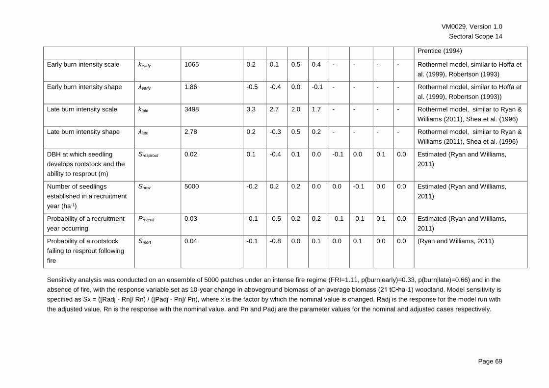
VM0029, Version 1.0

Sectoral Scope 14

Prentice (1994)

Early burn intensity scale kearly 1065 0.2 0.1 0.5 0.4 - - - - Rothermel model, similar to Hoffa et

al. (1999), Robertson (1993)

Early burn intensity shape λearly 1.86 -0.5 -0.4 0.0 -0.1 - - - - Rothermel model, similar to Hoffa et

al. (1999), Robertson (1993))

Late burn intensity scale klate 3498 3.3 2.7 2.0 1.7 - - - - Rothermel model, similar to Ryan &

Williams (2011), Shea et al. (1996)

Late burn intensity shape λlate 2.78 0.2 -0.3 0.5 0.2 - - - - Rothermel model, similar to Ryan &

Williams (2011), Shea et al. (1996)

DBH at which seedling

develops rootstock and the

ability to resprout (m)

Sresprout 0.02 0.1 -0.4 0.1 0.0 -0.1 0.0 0.1 0.0 Estimated (Ryan and Williams,

2011)

Number of seedlings

established in a recruitment

year (ha-1)

Snew 5000 -0.2 0.2 0.2 0.0 0.0 -0.1 0.0 0.0 Estimated (Ryan and Williams,

2011)

Probability of a recruitment

year occurring

Precruit 0.03 -0.1 -0.5 0.2 0.2 -0.1 -0.1 0.1 0.0 Estimated (Ryan and Williams,

2011)

Probability of a rootstock

failing to resprout following

fire

Smort 0.04 -0.1 -0.8 0.0 0.1 0.0 0.1 0.0 0.0 (Ryan and Williams, 2011)

Sensitivity analysis was conducted on an ensemble of 5000 patches under an intense fire regime (FRI=1.11, p(burn|early)=0.33, p(burn|late)=0.66) and in the

absence of fire, with the response variable set as 10-year change in aboveground biomass of an average biomass (21 tC•ha-1) woodland. Model sensitivity is

specified as Sx = ([Radj - Rn]/ Rn) / ([Padj - Pn]/ Pn), where x is the factor by which the nominal value is changed, Radj is the response for the model run with

the adjusted value, Rn is the response with the nominal value, and Pn and Padj are the parameter values for the nominal and adjusted cases respectively.

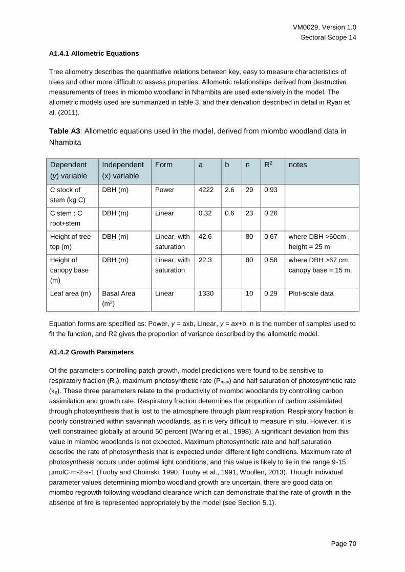
VM0029, Version 1.0

Sectoral Scope 14

A1.4.1 Allometric Equations

Tree allometry describes the quantitative relations between key, easy to measure characteristics of

trees and other more difficult to assess properties. Allometric relationships derived from destructive

measurements of trees in miombo woodland in Nhambita are used extensively in the model. The

allometric models used are summarized in table 3, and their derivation described in detail in Ryan et

al. (2011).

Table A3: Allometric equations used in the model, derived from miombo woodland data in

Nhambita

Equation forms are specified as: Power, y = axb, Linear, y = ax+b. n is the number of samples used to

fit the function, and R2 gives the proportion of variance described by the allometric model.

A1.4.2 Growth Parameters

Of the parameters controlling patch growth, model predictions were found to be sensitive to

respiratory fraction (Ra), maximum photosynthetic rate (Pmax) and half saturation of photosynthetic rate

(kp). These three parameters relate to the productivity of miombo woodlands by controlling carbon

assimilation and growth rate. Respiratory fraction determines the proportion of carbon assimilated

through photosynthesis that is lost to the atmosphere through plant respiration. Respiratory fraction is

poorly constrained within savannah woodlands, as it is very difficult to measure in situ. However, it is

well constrained globally at around 50 percent (Waring et al., 1998). A significant deviation from this

value in miombo woodlands is not expected. Maximum photosynthetic rate and half saturation

describe the rate of photosynthesis that is expected under different light conditions. Maximum rate of

photosynthesis occurs under optimal light conditions, and this value is likely to lie in the range 9-15

µmolC·m-2·s-1 (Tuohy and Choinski, 1990, Tuohy et al., 1991, Woollen, 2013). Though individual

parameter values determining miombo woodland growth are uncertain, there are good data on

miombo regrowth following woodland clearance which can demonstrate that the rate of growth in the

absence of fire is represented appropriately by the model (see Section 5.1).

Dependent

(y) variable

Independent

(x) variable

Form a b n R2 notes

C stock of

stem (kg C)

DBH (m) Power 4222 2.6 29 0.93

C stem : C

root+stem

DBH (m) Linear 0.32 0.6 23 0.26

Height of tree

top (m)

DBH (m) Linear, with

saturation

42.6 80 0.67 where DBH >60cm ,

height = 25 m

Height of

canopy base

(m)

DBH (m) Linear, with

saturation

22.3 80 0.58 where DBH >67 cm,

canopy base = 15 m.

Leaf area (m) Basal Area

(m2)

Linear 1330 10 0.29 Plot-scale data

VM0029, Version 1.0

Sectoral Scope 14

A1.4.3 Mortality & Regeneration Parameters

AGB change was found to be largely insensitive to parameters controlling miombo regeneration. Over

the time-scales of a REDD+ project, mechanisms of regeneration are not expected to be hugely

important as biomass change is concentrated in large stems which regenerate over several decades.

Over longer timescales it is expected that fire will reduce pressure on seedlings and sprouts by

exposing stems to lower intensity and less frequent fires. The lifting of this ‘demographic bottleneck’

should improve the capacity of woodlands to regenerate, though the impacts of these changes may

only be observable in the decades following fire management.

Stem mortality is of considerably greater importance to model output, particularly fire-induced top-kill.

This signals the importance of fire to the productivity of miombo woodlands. Data on fire dynamics in

miombo woodlands is scarce, though there is much information on fire behavior in savannah

grasslands, particularly from South Africa (Table 2). Fire intensity in miombo woodlands varies from

very low (<300 kW/m) to high intensity (>6,500 kW/m). There is also the potential for extremely high

intensity fires (>10,000 kW/m), though these have not been detected in miombo woodlands by

published fire experiments. Of particular significance are the results of Hoffa et al. (1999), where a

series of early-season fires in miombo woodlands showed a progression from very low intensities

through to the higher intensities observed by the mid dry season as described in figure A5.

Figure A5: Fire Intensity Measurements In Zambia From Hoffa Et Al. (1999), Showing a

Trend of Increasing Intensity through the Fire Season

Robertson (1993) also recorded the differences between early and late burns, measuring early burns

to be of very low intensity (<300 kW/m) and late burns to be considerably more intense and more

variable (500-5000 kW/m). Ryan and Williams (2011), setting fires in the late dry season, exploited

within fire variability at different times of day to achieve a wide range of fire intensities. Fires early in

the morning were of similar intensity to early burns (360 kW/m), with fire intensity reaching 6,600

kW/m at the hottest part of the day. Though currently available literature cannot provide all the

required detail about seasonal variability in fire intensity, it does give a suitable envelope of probable

fire intensities in miombo woodlands, as seen in table A2 below.

VM0029, Version 1.0

Sectoral Scope 14

Table A2: Observations of Fire Behaviour in Southern African Savannah and Miombo

Woodland Vegetation

Fuel

Type

Location ROS

(m/min)

Flame

Length (m)

Intensity

(kW/m)

Source

Miombo Mozambique 3 - 55 360 - 6600 (Ryan and Williams,

2011)

Savannah South Africa 0.6 - 102 28 - 17905 (Govender et al.,

2006)

Savannah Zambia 1.2 - 105.6 0.3 - 4.2 43 - 9476 (Hély et al., 2003)

Miombo Zambia 6 - 48 0.7 – 3.2 25 - 6553 (Hoffa et al., 1999)

Savannah South Africa 12 - 60 1 - 6 475 - 6130 (Shea et al., 1996)

Miombo Zambia 18 - 48 3 - 5 1734 - 4061 (Shea et al., 1996)

Savannah South Africa (Stocks et al., 1996)

Block 55 97.2 3.5 10906

Block 56 37.8 1.7 4048

Savannah South Africa 0.5 - 6 (Trollope et al., 1996)

Head 4.2 - 28.8 93 - 3644

Back 0.0 - 15 20 - 160

Miombo Zimbabwe

100 - 300

500 - 5000

(Robertson, 1993)

Early

Late

Acknowledgement: Bill Higham.

Further descriptors of fire seasonality may be generated using widely-used models of fire intensity.

The Rothermel model is a semi-empirical model of fire spread that has been widely used to

understand variation in fire intensity in a wide range of fire systems (Rothermel, 1972). Its equations

lie at the center of many modern fire models, including the United States Department of Agriculture

system for the evaluation of operational fire hazard (Pyne et al., 1996) and in the SPITFIRE module to

the LPJ dynamic global vegetation model (Thonicke et al., 2010). Its modest input requirements and

adaptability make it an appropriate means of approximating seasonal fire intensity variation in miombo

woodlands. The Rothermel model was parameterized using values from the literature as well as field

data from Kilwa, and driven by meteorological data from the ECMWF ERA-interim climate reanalysis

dataset and fuel curing estimates generated from the MODIS archive. The model arrangement is

described in appendix 2. The Rothermel output was used to generate distributions describing the

intensity of early and late burns as described in figure A6 below. Based on input data from 2000-2012

and an early/late cut-off date of the end of June, two Weibull distributions were fitted that qualitatively

fit expected fire intensities, with good matches for the expected seasonal fire intensity range. For each

early/late fire event, the model is set to randomly sample a fire intensity from these distributions.

VM0029, Version 1.0

Sectoral Scope 14

Figure 6: Normalized Histograms of Early and Late Fire Intensities Predicted ty the

Rothermel Model, Fitted With Weibull Distributions

Distributions are specified by scale (k) and shape (λearly) parameters, with values of kearly = 1065, klate =

1.86, λearly = 3498 and λlate = 2.78.

A1.5 Model Evaluation

A1.5.1 Patch Growth

Assumptions relating to growth parameters were validated using chronosequence field data from

Nhambita. A chronosequence is a series of forest sites with similar attributes that have been regrown

following clearance and abandonment, allowing the analysis of forest processes that occur over long

time scales, in this case forest regrowth. The chronosequence predicts approximately 0.7 tC/ha to be

accumulated each year on abandoned land which has not been observed to burn. This situation was

simulated by running the model from a start-point with no large stems through 25 years in the

absence of fire as decried in figure A7.

The model suggests a sigmoidal growth form, relating to exponentially increasing stand productivity

with biomass up to a saturation point. Average growth rates over 25 years produced by the model

amount to a biomass increment of 0.63 tC/ha, a rate slightly lower than observed in the

chronosequence. The model predicts basal area appropriately, with growth rate matching

observations. The model is less able to predict stocking density, likely due to the initialization of ‘bare’

patches with a stock of saplings, highlighting a limitation in the model representation of regeneration.

This data represents a conservative estimate of productivity as the annual increase in biomass is

VM0029, Version 1.0

Sectoral Scope 14

below that observed in miombo woodlands. Additionally, chronosequence observations are assumed

to be in the total absence of fire, which is unlikely to be the case in reality.

Figure 7: Model Output Comparison to Chronosequence Data from Nhambita

Biomass increase following abandonment is predicted accurately (RMSE = 5.3 tC/ha, R2=0.66), as is

basal area (RMSE = 1.7 m2/ha, R2=0.84), though the model is not able to very effectively capture

trends in stocking density of trees >5 cm DBH (RMSE = 250 ha-1, R2=0.53).

A1.5.2 Fire Intensity

It is not possible to fully evaluate performance of the Rothermel model due to the lack of appropriate

validation data from miombo woodlands. However, we are able to demonstrate that the predicted

intensities for early and late fires are reasonable, and thus result in a conservative rate of stem top-

kill. A review of the literature on miombo fires suggests that early burns have an intensity of less than

500 kW/m, whereas the Rothermel model predicts fire intensity to frequently rise above 1000 kW/m.

(For a REDD project, which expects to see an increase in early season fires, this higher average

intensity is conservative.)

Late season fires have a wider range of intensities, from 500 kW/m to over 6,000 kW/m, averaging

around 4,000 kW/m. The Rothermel model predicts a median late fire intensity of around 3,000 kW/m,

and that fire intensity very rarely rises above 6,000 kW/m. (Again for a REDD project, this is

conservative since it will result in using a less severe baseline scenario than is likely to be the case.).

VM0029, Version 1.0

Sectoral Scope 14

The Rothermel model estimate of fire intensity is based upon a fixed early/late cut-off date of the end

of June. In reality, climatic variability will shift this date annually, but purposive early burning can

generally be expected to produce lower intensity fires with consequent lower tree mortality.

A1.5.3 Exclusion of Dead Wood Pool

Analysis of the dead wood pool shows that it can be conservatively excluded as follows. The two

scenarios (baseline and project) are treated separately. Since excluding the pool is conservative for

both components, excluding it must be conservative overall.

A1.5.3.1 Baseline Scenario

At the start of project activities there will already be some dead wood present in the forest. This dead

wood pool will decay over a period of time releasing its carbon into the atmosphere. The rate of decay

will be affected by the fire regime; under the baseline scenario this does not change. The above

shows that harsh fire regimes such as pertain in the baseline scenario lead to a degradation in carbon

stocks, which scales with starting biomass. Thus, as the standing biomass declines, future additions

to the dead wood pool will be lower than previous additions to the pool. Since the rate of decay out of

the pool is constant, the carbon content of new additions each year will be lower than the amount lost

due to decay of existing dead wood. And thus excluding the dead wood pool conservatively estimates

actual carbon emissions in any given year.

A1.5.3.2 Project Scenario

Excluding the dead wood pool, and thus treating tree mortality as leading to instantaneous emissions

rather than the slow decay that actually takes place, will always be conservative in the Project

Scenario.

A1.5.4 Assessment of Model Conservativeness

Key to this modelling framework is the assertion that model predictions result in conservative

estimates of aboveground biomass change in all cases. From the model parameterization it can be

concluded that model outputs will result in conservative estimates of biomass change.

A1.5.4.1 Degradation

Tree top-kill from high intensity late-season fires dominates is higher in the baseline scenario than in

the project scenario, so in order to be conservative the model should under-estimate these losses.

Section 5.2 describes how the fire intensity used by the model is lower than that observed in reality.

Hence the model is conservative with respect to degradation.

5.4.2 Accumulation

Accumulation will be higher in the project scenario than in the baseline scenario, so in order to be

conservative the model should under-estimate these gains. Section 5.1 shows that modelled

woodland productivity is below that observed in miombo woodlands, and therefore estimated biomass

accumulation rates are likely lower than those that will be observed in reality. Hence the model is

conservative with respect to accumulation.

VM0029, Version 1.0

Sectoral Scope 14

A1.6 Using the Model

The model has been ported into Microsoft Excel as a familiar environment for users to examine

detailed model outputs. The spreadsheet provided does not contain any of the model itself, but is an

interface for setting model parameters and visualizing outputs. The spreadsheet allows for simple use

of commonly used model functions, and also analysis of the impact of parameter changes and the

exploration of raw data outputs. Here we describe use of the model for prediction of carbon storage

changes from a modified fire regime.

The model is provided in a compressed folder (‘GapFire.zip’), and should be unzipped to the C:\ drive.

Open ‘GapFire.xlsm’ to access the model spreadsheet, dismissing the security warning that appears

at the top of the workbook (‘Enable Content’). The primary controls for the model are number of

ensembles (‘patches’), project start date, initial biomass, and frequency of early and late fires in the

baseline and project scenarios as described in figure A8 below. Increasing the number of patches will

result in a less variable output, but will increase model run time. A minimum of 10,000 patches should

be used to achieve a reliable model run, with 100,000 patches recommended. Initial biomass can be

altered to reflect the mean starting biomass of patches. Due to the random allocation of stems to each

patch the actual initial biomass may be slightly different to that selected, but such differences are

minimal when a large number of patches are run.

Figure A8: Primary inputs to the model for use in carbon accounting

Fire frequency should be input based on historical fire mapping and ongoing monitoring. The model

should be started from the year the data for the carbon density map was obtained; this may predate

the start of project activities for a few years; the number of years after the map date must be entered

as the Project Start. The baseline fire scenario must then be copied into the relevant cells of the

project fire regime. The actual fire frequency for each year of project activities as determined by

monitoring must then be input into the appropriate cells. Years which are left blank relate to future

years; the model will compute the mean fire frequencies since the start of project activities and use

them to predict performance up to year 10. Note that the probability of no fire is equal to 1 – pEarly –

pLate.

To run the model, the parameter input file should first be updated using ‘Update Parameters’, which

writes selected parameters to a comma separated variables (.csv) file. The model is started using

VM0029, Version 1.0

Sectoral Scope 14

‘Run GapFire’ and once complete the spreadsheet should be updated with new model outputs using

‘Update Results’ as described in figure A9.

Figure A9: Model Controls, Initiating 1) Writing of Model Input File, 2) Model Run, and 3)

Spreadsheet Update

Model outputs are summarised in a table showing aboveground carbon storage in the baseline and

project scenarios, along with estimates of avoided emissions, sequestered carbon and net change as

described in figure A10. This summary contains the information required for a REDD+ project to

account for aboveground biomass change.

Figure A10: Summary of Carbon Storage Change Predicted by the Model

A graphical summary of carbon storage change in the project and baseline scenarios is also

generated, as well as estimates of carbon storage change between the two scenarios and the rate of

carbon accumulation as described in figure A11 below. Avoided emissions are calculated as the

difference between initial biomass and baseline predicted biomass, and sequestered carbon is

computed as the increase in aboveground biomass in the project scenario since model initialization.

All data is presented in a raw format to allow for more detailed analysis of potential project impacts.

Further information is presented on the ‘Parameters’ worksheet, where model parameters and

variables can be altered. Raw model outputs are displayed in the ‘DATA’ worksheet, where additional

model outputs can be explored. For a more advanced user, model code is supplied written in Fortran

90, which may be compiled to the project’s specification.

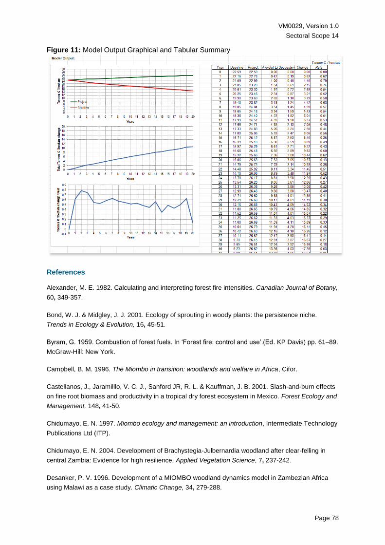
VM0029, Version 1.0

Sectoral Scope 14

Figure 11: Model Output Graphical and Tabular Summary

References

Alexander, M. E. 1982. Calculating and interpreting forest fire intensities. Canadian Journal of Botany,

60, 349-357.

Bond, W. J. & Midgley, J. J. 2001. Ecology of sprouting in woody plants: the persistence niche.

Trends in Ecology & Evolution, 16, 45-51.

Byram, G. 1959. Combustion of forest fuels. In ‘Forest fire: control and use’.(Ed. KP Davis) pp. 61–89.

McGraw-Hill: New York.

Campbell, B. M. 1996. The Miombo in transition: woodlands and welfare in Africa, Cifor.

Castellanos, J., Jaramilllo, V. C. J., Sanford JR, R. L. & Kauffman, J. B. 2001. Slash-and-burn effects

on fine root biomass and productivity in a tropical dry forest ecosystem in Mexico. Forest Ecology and

Management, 148, 41-50.

Chidumayo, E. N. 1997. Miombo ecology and management: an introduction, Intermediate Technology

Publications Ltd (ITP).

Chidumayo, E. N. 2004. Development of Brachystegia-Julbernardia woodland after clear-felling in

central Zambia: Evidence for high resilience. Applied Vegetation Science, 7, 237-242.

Desanker, P. V. 1996. Development of a MIOMBO woodland dynamics model in Zambezian Africa

using Malawi as a case study. Climatic Change, 34, 279-288.

VM0029, Version 1.0

Sectoral Scope 14

Desanker, P. V. & Prentice, I. C. 1994. MIOMBO – A vegetation dynamics model for the miombo

woodlands of Zambezian Africa. Forest Ecology and Management, 69, 87-95.

Goldammer, J. G. & De Ronde, C. 2004. Wildland fire management handbook for Sub-Sahara Africa,

African Minds.

Govender, N., Trollope, W. S. & Van Wilgen, B. W. 2006. The effect of fire season, fire frequency,

rainfall and management on fire intensity in savanna vegetation in South Africa. Journal of Applied

Ecology, 43, 748-758.

Hély, C., Alleaume, S., Swap, R. & Justice, C. 2003. SAFARI-2000 characterization of fuels, fire

behavior, combustion completeness, and emissions from experimental burns in infertile grass

savannas in western Zambia. Journal of Arid Environments, 54, 381-394.

Hendricks, J. J., Hendrick, R. L., Wilson, C. A., Mitchell, R. J., Pecot, S. D. & Guo, D. 2006. Assessing

the patterns and controls of fine root dynamics: an empirical test and methodological review. Journal

of Ecology, 94, 40-57.

Jackson, J. F., Adams, D. C. & Jackson, U. B. 1999. Allometry of constitutive defense: A model and a

comparative test with tree bark and fire regime. American Naturalist, 153, 614-632.

Johnson, E. A. & Miyanishi, K. 2001. Forest fires: behavior and ecological effects, Academic Press

San Diego, CA.

Jones, H. G. 1992. Plants and microclimate: a quantitative approach to environmental plant

physiology, Cambridge University Press.

Miller, C. & Urban, D. L. 2000. Modeling the effects of fire management alternatives on Sierra Nevada

mixed-conifer forests. Ecological Applications, 10, 85-94.

Mlambo, D. & Mapaure, I. 2006. Post-fire resprouting of Colophospermum mopane saplings in a

southern African savanna. Journal of Tropical Ecology, 22, 231-234.

Norman, J. M. & Campbell, G. S. 1991. Canopy structure. Plant physiological ecology. Springer.

Nottingham, A. 2004. The characterisation of foliar N-concentrations and presence of N-fixers in

Miombo woodland, Mozambique. MRes, University of Dundee.

Pyne, S. J., Andrews, P. L. & Laven, R. D. 1996. Introduction to wildland fire, John Wiley and Sons.

Robertson, F. E. 1993. Early-burning in the Brachystegia woodland of the Parks and Wild Life Estate.

Zimbabwe Science News, 27, 68-71.

Rothermel, R. C. 1972. A mathematical model for predicting fire spread in wildland fuels, USFS.

Running, S. W., Nemani, R. R. & Hungerford, R. D. 1987. Extrapolation of synoptic meteorological

data in mountainous terrain and its use for simulating forest evapotranspiration and photosynthesis.

Canadian Journal of Forest Research, 17, 472-483.

VM0029, Version 1.0

Sectoral Scope 14

Ryan, C. M. & Williams, M. 2010. How does fire intensity and frequency affect miombo woodland tree

populations and biomass? Ecological Applications, 21, 48-60.

Ryan, C. M., Williams, M. & Grace, J. 2011. Above‐and Belowground Carbon Stocks in a Miombo

Woodland Landscape of Mozambique. Biotropica, 43, 423-432.

Saito, M., Poulter, B., Bellassen, V., Yue, C., Ryan, C. M., Williams, M., Luysseart, S., Ciais, P. &

Peylin, P. in prep. Fire regimes and variability in above ground woody biomass in an African savanna

woodland.

Shea, R. W., Shea, B. W., Kauffman, J. B., Ward, D. E., Haskins, C. I. & Scholes, M. C. 1996. Fuel

biomass and combustion factors associated with fires in savanna ecosystems of South Africa and

Zambia. Journal of Geophysical Research: Atmospheres, 101, 23551-23568.

Shugart, H. H. & Smith, T. M. 1996. A review of forest patch models and their application to global

change research. Climatic Change, 34, 131-153.

Stocks, B., Van Wilgen, B., Trollope, W., Mcrae, D., Mason, J., Weirich, F. & Potgieter, A. 1996. Fuels

and fire behavior dynamics on large-scale savanna fires in Kruger National Park, South Africa.

Journal of Geophysical Research, 101, 23541-23,550.

Sutherland, E. K. & Smith, K. T. 2000. Resistance is not futile: the response of hardwoods to fire-

caused wounding. In: Proceedings: workshop on fire, people, and the central hardwood landscape.

General Technical Report NE-274, US Department of Agriculture, Forest Service, Northeastern Forest

Experiment Station, Newtown Square, PA, 2000. 111-115.

Trollope, W., Trollope, L., Potgieter, A. & Zambatis, N. 1996. SAFARI-92 characterization of biomass

and fire behavior in the small experimental burns in the Kruger National Park. Journal of Geophysical

Research, 101, 23531-23,539.

Tuohy, J. & Choinski, J. 1990. Comparative photosynthesis in developing leaves of Brachystegia

spiciformis Benth. Journal of Experimental Botany, 41, 919-923.

Tuohy, J. M., Prior, J. A. & Stewart, G. R. 1991. Photosynthesis in relation to leaf nitrogen and

phosphorus content in Zimbabwean trees. Oecologia, 88, 378-382.

Waring, R., Landsberg, J. & Williams, M. 1998. Net primary production of forests: a constant fraction

of gross primary production? Tree Physiology, 18, 129-134.

Williams, M. 1996. A three-dimensional model of forest development and competition. Ecological

Modelling, 89, 73-98.

Woollen, E. 2013. Carbon dynamics in African miombo woodlands: from the leaf to the landscape.

PhD, Edinburgh University.

Design credits: Figure 1, Horhew & redheadstock (deviantART.com).

VM0029, Version 1.0

Sectoral Scope 14

APPENDIX 2: THE ROTHERMEL MODEL

This appendix was prepared by Sam Bowers and Prof. Mathew Williams of the University of

Edinburgh.

Rothermel’s model simulates fire as a quasi-steady state series of ignitions in a spatially uniform

fuelbed. Rate of fire spread is modelled as the ratio of propagating heat flux to the energy required to

dry out and ignite unburned fuels. Fire rate of spread is influenced by the geometry, composition and

moisture content of the fuelbed, and multiplicative factors describing wind speed and slope. The

complete Rothermel model of fire spread is:

𝑅 =

𝐼𝑅𝜉(1 + 𝜙𝑤 + 𝜙𝑠)

𝜌𝑏𝜀𝑄𝑖𝑔 (1)

where R = rate of spread (m min-1), IR = reaction intensity of the flaming front (kJ m-2 min-1), ξ =

propagating flux ratio (dimensionless), φw = wind coefficient (dimensionless), φw = slope coefficient

(dimensionless), ρB = fuelbed bulk density (kg m-3), ε = effective heating number (proportion of fuel

raised to ignition temperature) (dimensionless), and Qig = heat of pre-ignition (quantity of heat

required to ignite fuel, a function of moisture content) (kJ kg-1). Reaction intensity (IR) is the product of

several factors that relate to rate of energy release, specified by:

𝐼𝑅 = Γ′𝑊𝑛ℎ𝜂𝑀𝜂𝑠 (2)

where Γ’ = optimum reaction velocity (min-1), Wn = net fuel loading (kg m-2), h = low heat content (kJ

kg-1), ηM = moisture damping coefficient and ηs = mineral damping coefficient. Reaction velocity is

calculated as a function of surface area to volume ratio (σ). For further information on the formulation

of the Rothermel model, refer to Rothermel (1972). Importantly, the Rothermel model can be applied

to estimate of fireline intensity by combining modelled rate of spread with combustion completeness

(Cf), here estimated using the method of Peterson and Ryan (1986):

1-hr

fuels:

𝑖𝑓 𝑚𝑓

𝑚𝑒𝑥𝑡≤ 0.18, 𝐶𝑓 = 1.0

𝑖𝑓 0.18 <𝑚𝑓

𝑚𝑒𝑥𝑡≤ 0.73, 𝐶𝑓 = 1.2 − 0.62

𝑚𝑓

𝑚𝑒𝑥𝑡

𝑖𝑓 𝑚𝑓

𝑚𝑒𝑥𝑡> 0.73, 𝐶𝑓 = 2.45 − 2.45

𝑚𝑓

𝑚𝑒𝑥𝑡

(3)

10-hr

fuels:

𝑖𝑓 𝑚𝑓

𝑚𝑒𝑥𝑡≤ 0.12, 𝐶𝑓 = 1.0

𝑖𝑓 0.12 <𝑚𝑓

𝑚𝑒𝑥𝑡≤ 0.51, 𝐶𝑓 = 1.09 − 0.72

𝑚𝑓

𝑚𝑒𝑥𝑡

𝑖𝑓 𝑚𝑓

𝑚𝑒𝑥𝑡> 0.51, 𝐶𝑓 = 1.47 − 1.47

𝑚𝑓

𝑚𝑒𝑥𝑡

(4)

VM0029, Version 1.0

Sectoral Scope 14

100-

hr

fuels:

𝑖𝑓 0𝑚𝑓

𝑚𝑒𝑥𝑡≤ 0.38, 𝐶𝑓 = 0.98 − 0.85

𝑚𝑓

𝑚𝑒𝑥𝑡

𝑖𝑓 𝑚𝑓

𝑚𝑒𝑥𝑡> 0.38, 𝐶𝑓 = 1.06 − 1.06

𝑚𝑓

𝑚𝑒𝑥𝑡

(5)

Where mf = moisture content of fuel (dimensionless) and mext = fuel moisture of fire extinction

(dimensionless). Fuels are split into three size classes: 1-hour - <0.64cm, 10-hour – 0.64-2.5cm, 100-

hour – 2.5cm-7.5cm, which each have characteristic surface are to volume ratio and drying rates. The

1-hr fuel class is split into live (green grass) and dead (dry grass, litter) classes, which have distinct

behaviors. The input of each fuel class to the overall rate of spread is calculated by weighting the

different fuel classes by their surface area to volume ratios.

The Rothermel model requires a number of inputs to predict fire intensity, summarized in table A4

below. These have been selected from a combination of field measurements and standardized

parameters from the literature. In addition to fixed fuel parameters, a number of inputs will be

expected to change seasonally, namely fuel curing, fuel moisture and windspeed. These drivers are

estimated as follows:

Fuel Curing: Annual curing (drying) of grass fuels is one of the key influences on annual fire intensity

variation in miombo woodlands (Hoffa et al., 1999). The proportion of grass that is cured is

approximated using NDVI measurements from MODIS, covering areas of Kilwa within the 5-35 tC/ha

biomass range. As the relationship between NDVI and fuel curing is often inconsistent between

locations, a ‘relative greenness’ value is calculated based on the maximum and minimum recorded

NDVI value in each pixel (j):

𝑅𝐺𝑖,𝑗 =

𝑁𝐷𝑉𝐼𝑖,𝑗 − 𝑁𝐷𝑉𝐼𝑚𝑖𝑛,𝑗

𝑁𝐷𝑉𝐼𝑚𝑎𝑥,𝑗 − 𝑁𝐷𝑉𝐼𝑚𝑖𝑛,𝑗 (6)

where i is the time of measurement and NDVImax,j and NDVImin,j are the maximum and minimum NDVI

values recorded at each pixel over a specified time period. This time period was set to 3 years to

maximize the chances of capturing extremes of NDVI whilst minimizing the impact of land cover

changes on the predictions of fuel curing (Newnham et al., 2011). This method is similar to that used

in Australia’s Grassland Fire Index and the United States National Fire Danger Rating System

(NFDRS) (Burgan et al., 1998).

Fuel Moisture: Fuel moisture of dead fuel varies through the year based on rainfall events and

subsequent drying. Dead fuel moisture is estimated using the method of Thonicke et al. (2010), which

is based upon calculation of the Nesterov Index of fire danger (Nesterov, 1949):

𝑁𝐼(𝑑) = ∑ 𝑇𝑚𝑎𝑥(𝑑) ∙ (𝑇𝑚𝑎𝑥(𝑑) − 𝑇𝑑𝑒𝑤(𝑑)) (7)

where Tmax(d) is the maximum temperature and Tdew(d) is the dew point at day d and summation is

over the number of consecutive days that precipitation remains <3mm. When a day receives >3mm

precipitation, the Nestrov Index resets to 0. Temperature and precipitation data are taken from the

VM0029, Version 1.0

Sectoral Scope 14

ERA-interim climate reanalysis dataset, and Tdew(d) is approximated as Tmin(d) – 4 (Running et al.,

1987) where Tmin is the minimum daily temperature. Moisture content for each fuel class is calculated

as:

𝜔𝑖 = 𝑒−𝛼𝑖 ∙ 𝑁𝐼(𝑑) (8)

where ωi = relative fuel moisture of size class i, and αi is applied to the three fuel classes in inverse

proportion to the surface area to volume ratios (α1h = 1.0 ⋅ 10−3, α10h = 5.42 ⋅ 10−5, α100h = 1.49 ⋅ 10−5).

Live fuel moisture is estimated from degree of curing, where a maximum greenness related to 230

percent moisture content, and minimum curing to 30 percent moisture content, where live fuels

behave in the same manner as dead fuels. As a dynamic fuel model, fuel is transferred from the live

to the dead class in proportion to the quantity of the grass fuel that is cured (Scott and Burgan, 2005).

Wind Speed: Wind has a considerable impact on fire behavior, with stronger winds relating to a more

intense fire. Wind speed at 10m is used from the ERA-interim dataset, and adjusted by a factor of

0.45 to represent the reduction of wind speed within woodlands.

VM0029, Version 1.0

Sectoral Scope 14

Table A4: Rothermel model parameters

Response variables are median early/late fire intensity. Model sensitivity is specified as Sx = ([Radj - Rn]/ Rn) / ([Padj - Pn]/ Pn), where x is the factor by which the

nominal value is changed, Radj is the response for the model run with the adjusted value, Rn is the response with the nominal value, and Pn and Padj are the

parameter values for the nominal and adjusted cases respectively.

Early Late

Parameter

Description

Parameter Name Nominal Value S0.5 S0.75 S1.5 S2 S0.5 S0.75 S1.5 S2 Source

Fuel mass (kg m-2)

● grass

● 1hr (other)

● 10hr

● 100hr

Wlive

W1-hr

W10-hr

W100-hr

0.59

0.11

0.05

0.06

0.8

0.1

0.0

-0.1

0.7

0.1

0.0

-0.1

0.9

0.2

0.0

-0.1

0.8

0.2

0.0

-0.1

1.0

0.0

0.0

0.0

1.0

0.0

0.0

0.0

1.0

0.0

0.0

-0.1

1.0

0.1

0.0

0.0

Field measurements (Kilwa).

Surface area to volume

ratio (cm-1)

● grass

● 1hr (other)

● 10hr

● 100hr

σlive

σ1-hr

σ10-hr

σ100-hr

59.74

65.5

3.58

0.98

0.2

0.1

0.0

0.0

0.2

0.2

0.0

0.0

0.5

0.3

0.0

0.0

0.5

0.3

0.0

0.0

0.5

0.0

0.0

0.0

0.5

0.1

0.0

0.0

0.3

0.1

0.0

0.0

0.7

0.2

0.0

0.0

Field measurements (Nhambita).

(σlive, σ1-hr)

(Scott and Burgan, 2005) (σ10-hr,

σ100-hr)

Fuelbed depth (m) δ 0.45 1.0 1.0 1.0 1.0 1.1 1.1 1.1 1.1 Field measurements (Kilwa)

Wind adjustment factor wadj 0.45 1.1 1.2 1.4 1.5 1.2 1.3 1.5 1.6 Estimated, similar to Thonicke et al.

(2010)

Max living fuel moisture ωmax 120% -0.9 -0.9 -0.5 -0.3 -0.3 -0.3 -0.2 -0.2 Scott and Burgan 2005)

Min living fuel moisture ωmin 30% -0.1 -0.1 -0.1 -0.1 -0.1 -0.1 -0.1 -0.1 Scott and Burgan 2005)

Fuel heat content (kJ

kg-1)

h 18,622 1.5 1.7 2.4 2.7 1.5 1.7 2.5 3.0 Scott and Burgan 2005)

VM0029, Version 1.0

Sectoral Scope 14

Fuel particle density (kg

m-3)

ρp 513 0.1 0.1 0.0 0.0 0.1 0.1 0.0 0.0 Scott and Burgan 2005)

Minimum fireline

intensity for continued

combustion (kW/m)

Imin 50 0.0 0.0 0.0 0.0 0.0 0.0 0.0 0.0 Estimated

By running the model on a daily time step for all years of available data (2000-2012), a clear fire season

is predicted beginning in mid-May, lasting through to December (Figure 12). Fire intensity is predicted to

remain low in May/June, peak in September and reduce towards the end of the year. The model suggests

that fire intensity is highly variable at any given time of year, though average intensity of late season fires

are significantly greater than early season fires. By splitting these predicted fire intensities into ‘early’ (day

≤180) and ‘late’ (day>180) season fires, two different fire intensity PDFs were produced figure 12.

Figure 12: Predictions of Fire Seasonality from the Rothermel Model

Individual years (2000-2012) are plotted in grey and the mean of all years plotted in red.

References

Burgan, R. E., Klaver, R. W. & Klaver, J. M. 1998. Fuel models and fire potential from satellite and surface observations. International Journal of Wildland Fire, 8, 159-170.

Hoffa, E. A., Ward, D., Hao, W., Susott, R. & Wakimoto, R. 1999. Seasonality of carbon emissions from biomass burning in a Zambian savanna. Journal of Geophysical Research: Atmospheres, 104, 13841-13853.

Nesterov, V. 1949. Combustibility of the forest and methods for its determination. Moscow: Goslesbumaga.

Newnham, G. J., Verbesselt, J., Grant, I. F. & Anderson, S. A. 2011. Relative greenness index for assessing curing of grassland fuel. Remote Sensing of Environment, 115, 1456-1463.

Peterson, D. L. & Ryan, K. C. 1986. Modeling postfire conifer mortality for long-range planning. Environmental Management, 10, 797-808.

Rothermel, R. C. 1972. A mathematical model for predicting fire spread in wildland fuels, USFS.

Running, S. W., Nemani, R. R. & Hungerford, R. D. 1987. Extrapolation of synoptic meteorological data in mountainous terrain and its use for simulating forest evapotranspiration and photosynthesis. Canadian Journal of Forest Research, 17, 472-483.

Scott, J. H. & Burgan, R. E. 2005. Standard fire behavior fuel models: a comprehensive set for use with Rothermel's surface fire spread model. The Bark Beetles, Fuels, and Fire Bibliography, 66.

Thonicke, K., Spessa, A., Prentice, I., Harrison, S., Dong, L. & Carmona-Moreno, C. 2010. The influence of vegetation, fire spread and fire behaviour on biomass burning and trace gas emissions: results from a process-based model. Biogeosciences, 7, 1991-2011.

DOCUMENT HISTORY

Version Date Comment

v1.0 8 May 2015 Initial version

Methodology for Avoided Degradation through Fire Management

Documents

Transcript of Methodology for Avoided Degradation through Fire Management