Methodologies and Tools for Forecasting Infrastructure · Methodologies and Tools for Forecasting...

4

Patterns of Potential Human Progress Volume 4: Building Global Infrastructure76

Methodologies and Tools for Forecasting Infrastructure

as a bridge between the largely conceptual discussion of chapter 3 and the forecasting analyses to come, this chapter turns to the more technical topic of how we can best forecast global infrastructure futures. the choice of the most appropriate tools and methods depends on a number of factors. What aspects of infrastructure are to be considered—the size of the physical stock, annual additions, the amount of spending required, the breakdown of spending into construction and maintenance, sources and availability of funding, or the impacts of infrastructure on other systems? What specific types of infrastructure are to be modeled and at what level of detail—for example, total electricity generation capacity or capacity by specific type of power plant? What is the time horizon of interest—one year, ten years, fifty years, or one hundred years? What is the geographic scope of interest—a city, a country, a region, or the world?

As discussed in Chapter 1, we set out to explore five key questions in this volume. First, we asked what a likely infrastructure future might be based on the interaction of demand and supply-side forces. Second, we wondered how such a future might impact access rates around the world. Third, how might the forecasted changes to infrastructure stocks, access, and spending impact future levels of human development? Fourth, given their economic and social implications, are today’s existing goals for improving infrastructure access realistic for all countries? And finally, if the answer to that last question is no, can we instead develop a set of aggressive but more reasonable targets that enable countries to provide important infrastructure services to more of their citizens? Addressing these five questions requires us to be able to forecast the demand for infrastructure, the ability of countries to meet such demands, and the broader socioeconomic and environmental implications associated with alternative

This chapter turns to the more technical topic of how we can best forecast global infrastructure

futures.

Methodologies and Tools for Forecasting Infrastructure 77

infrastructure forecasts (including feedbacks to the explanatory variables, or drivers, of infrastructure demand and supply).

Figure 4.1 elaborates the earlier Figure 1.4 to provide an overview of the dynamic, integrated, infrastructure forecasting model we have developed for this volume. As with the poverty, education, and health models described in the previous Patterns of Potential Human Progress volumes, this infrastructure model is integrated into the complete International Futures (IFs) system. We describe that larger system in the next section of this chapter.

The integrated IFs system begins its infrastructure forecasts with expected levels of infrastructure based on a country’s general level of development. These expected levels are then used in conjunction with assumptions about costs to estimate the funding required for maintaining existing infrastructure and constructing new infrastructure to meet these expectations. We estimate the funding available for infrastructure separately. Since there is no guarantee that the available funding will match exactly the funding required for expected levels of infrastructure, the actual level of infrastructure can (and often does) differ from the expected level. These actual levels then feed forward to affect various aspects of human development and well-being, which, in turn, feed back to the determinants of expected levels of infrastructure and the availability of funding

in future years. These determinants also evolve over time in response to many factors that are addressed in other parts of IFs but are not shown in Figure 4.1.

This chapter fleshes out many of the details of the IFs infrastructure modeling system. As with most modeling endeavors, we owe a great debt to others whose past and ongoing work we have learned from, adapted, and extended. A review of a number of these efforts follows a brief introduction to the IFs system.

Integrating Infrastructure with Broader Human Development: The Larger IFs SystemIFs is a large-scale, long-term, integrated global modeling system. It represents demographic, economic, educational, health, energy, agricultural, sociopolitical, and environmental subsystems for 183 interacting countries.1 The model system itself runs in annual time steps from its initial year (currently 2010) with user-defined time horizons ranging out to 2100.2 The central purpose of IFs is to facilitate exploration of global futures through alternative scenarios.

The goals that motivated the design of IFs fall generally into three categories: human development, social fairness and security, and environmental sustainability. Across these domains, the project draws inspiration from seminal writers such as Sen (1999) with his emphasis on freedom and individual

IFs is a large-scale,

long-term, global modeling system

that includes 183 countries.

Figure 4.1 The dynamic, integrated, infrastructure modeling system in IFs

Determinants ofexpected levelsof infrastructure

Expected levelsof infrastructure

Unit costs ofinfrastructure

Funding requirementsfor expected levels

of infrastructure

Funding availablefor infrastructure

Determinants offunding availablefor infrastructure

Actual funding forinfrastructure

Actual level ofinfrastructure

Socioeconomic andenvironmental effects

of infrastructure

Source: Authors’ conceptualization.


development, Rawls (1971) with his emphasis on fairness within society, and Brundtland (World Commission on Environment and Development 1987) with her foundational definition of sustainability. In combination, these emphases provide a philosophical framework for the exploration of human beings as individuals, of human beings with each other, and of human beings with the environment.

Fundamentally, IFs is a thinking tool, allowing variable time horizons through 2100 for exploring human agency in pursuit of key goals in the face of great uncertainty. IFs assists with:

■■ understanding the state of the world and the future that appears to be unfolding

■■ identifying tensions and inconsistencies that suggest political, economic, or other risks in the near and middle term (a “watch list” functionality);

■■ exploring longer-term trends and considering where they might be taking us;

■■ working through the complex dynamics of global systems.

■■ thinking about the future we want to see■■ clarifying goals and priorities;■■ developing alternative scenarios (“if-then

statements”) about the future;■■ investigating the leverage we may have in

shaping the future.

Human systems fundamentally involve agents (economists often represent them as individuals in households or firms; political scientists add governments) interacting with each other in various structures (economists focus on markets; political scientists look to action-reaction systems and international regimes; sociologists add societies and demographic structures; anthropologists focus on cultures; physical scientists extend the reach to ecosystems). In general, social scientists seek to understand the co-creation and evolution of such agent behaviors and structural characteristics.

IFs attempts to capture some of the richness of such systems. It is a structure-based (with extensive representation of underlying accounting systems, such as demographic structures and the exchanges of goods,

services, and finance), agent-class driven (so as to provide a basis for representing change), dynamic modeling system. That is, IFs represents typical behavior patterns of major agent-classes (households, governments, firms) interacting in a variety of global structures (demographic, economic, social, and environmental). The system draws on standard approaches to modeling specific issue areas whenever possible, extending those as necessary and integrating them across issue areas. For instance, the demographic model uses the typical cohort-component representation, tracking country-specific populations over time by age and sex (extended by education). Within that structural or accounting framework, the model represents the fertility decisions of households (influenced by income and education), as well as mortality and migration patterns. Similarly with respect to health, we have attempted to build on existing approaches—particularly that of the World Health Organization’s Global Burden of Disease project (Mathers and Loncar 2006; Mathers and Loncar updated n.d.)—extending those as possible and integrating them with the larger IFs system.

As well as being rooted in the theory of various disciplines and subspecializations, IFs is heavily data-driven. Data come from the various member organizations of the United Nations family and many other sources. The database underlying IFs, and integrated with the system for use by others, includes data for 183 countries over as much of the period since 1960 as possible.

Figure 4.2 shows the major conceptual blocks of the IFs system. The elements of the technology block are, in fact, scattered throughout the model, as are many elements of the infrastructure model, and for the same reason: both are fundamental underlying systems. The named linkages between blocks are a very small illustrative subset, not an exhaustive listing.

The population and economic models form the core of the IFs system. Some of the key characteristics of the population model are that it:

■■ represents 22 age-sex cohorts to age 100+ in a standard cohort-component structure (but computationally spreads the five-year cohorts

IFs represents typical behavior

patterns of major agent-classes, such

as households, governments,

and firms, as they interact in a variety of global structures

and systems.


initially to one-year cohorts and calculates change in one-year time steps);

■■ calculates change in cohort-specific fertility of households in response to income, income distribution, infant mortality (from the health model), education levels, and contraception use;

■■ uses mortality calculations from the health model;

■■ separately represents the evolution of HIV infection rates and deaths from AIDS;

■■ computes average life expectancy at birth, literacy rate, and overall measures of human development;

■■ represents migration, which ties to flows of remittances.

Some of the most important characteristics of the economic model are that it:

■■ represents the economy in six sectors: agriculture, materials, energy, industry, services, and information and communication technologies (ICT);

■■ computes and uses input-output matrices that change dynamically with development level;

■■ is a general equilibrium-seeking model that does not assume exact equilibrium will exist in any given year; rather it uses inventories as buffer stocks and to provide price signals so that the model chases equilibrium over time;

■■ contains a Cobb-Douglas production function that, following insights of Solow and Romer (see Romer 1990; 1994), endogenously represents contributions to growth in multifactor productivity from human capital (education and health), social capital and governance, physical and natural capital (infrastructure and energy prices), and knowledge development and diffusion (research and development [R&D] and economic integration with the outside world);

■■ uses a linear expenditure system (LES) to represent changing consumption patterns;

■■ utilizes a pooled-trade approach for international trade;

■■ is embedded in a social accounting matrix (SAM) envelope that ties economic production and consumption to representation of intra-actor financial flows.

The sociopolitical model interacts with the infrastructure model as well as with the economic, demographic, health, and education models. Some of its relevant features are that it:

■■ represents fiscal policy through taxing and spending decisions;

■■ shows seven categories of government spending: military, health, education, R&D, infrastructure (core), infrastructure other, and a residual category;

■■ represents changes in social conditions of individuals (such as fertility rates, literacy levels, or poverty), attitudes of individuals (such as the level of materialism/post-materialism of a society from the World Values Survey), and the social organization of people (such as the status of women);

Figure 4.2 Major models in the IFs modeling system and example connections

Sociopolitical International political

Education Health

Population Economy

Agriculture Energy

Technology Environmental resourcesand quality

Infrastructure

Governmentexpenditures

Conflict/cooperationStability/instability

Mortality

Income

Demand,supply, prices,

investment

Fertility

Labor

EfficienciesLand useWater use

Resource useCarbon production

Fooddemand

Links shown are examples from much larger set



■■ represents the evolution of democracy and governance-character variables such as effectiveness and corruption level;

■■ represents the prospects for state instability or failure.

The environmental model of IFs is not as developed as that of many integrated assessment models, but among its capabilities it:

■■ forecasts exposure to indoor air pollution from the use of solid fuels for heating and cooking;

■■ computes outdoor particulate concentrations for urban areas;

■■ forecasts atmospheric accumulations of carbon dioxide from fossil fuel use and deforestation, and replicates findings from more extensive general circulation models to compute associated changes in temperature and precipitation at the national level that, in turn, affect crop yields.

Although IFs was initially developed as an educational tool, it increasingly supports research and policy analysis. (See the volume preface for information on our flagship series, Patterns of Potential Human Progress, of which this volume is a part.) IFs was a core component of a project exploring the New Economy sponsored by the European Commission in the TERRA project (B. Hughes and Johnson 2005) and a subsequent European Commission project on information and communication technologies and sustainability (Moyer and B. Hughes 2012). Forecasts from IFs supported Project 2020 (Mapping the Global Future) of the U.S. National Intelligence Council (USNIC 2004), Global Trends 2025 (USNIC 2008), and the most recent report of the National Intelligence Council, Global Trends 2030: Alternative Worlds (USNIC 2012). IFs also provided driver forecasts and some integrating analysis for GEO-4, the fourth Global Environment Outlook of the United Nations Environment Programme (UNEP 2007), as well as scenarios on environmental challenges to human development for the 2011 Human Development Report (B. Hughes, Irfan, et al. 2011). In addition, it was used as the primary tool for the African Futures 2050 project funded by the British High Commission and based at the Institute for Security Studies in South Africa (Cilliers, B. Hughes, and Moyer 2011).

The menu-driven interface of the IFs software system allows display of historical data since 1960 (in most cases) in combination with results from a Base Case and from alternative scenarios over time horizons from 2010 through 2100, facilitating user interventions flexibly across time, issue area, and geography. The system facilitates scenario development and policy analysis via a scenario tree that simplifies changes in framing assumptions and agent-class interventions. Users can save scenarios for development and refinement over time. Standard framing scenarios (such as those from the United Nations Environment Programme GEO-4 report) are available with the model for users to explore and potentially develop further. Displays include tables, standard graphical formats, and a basic Geographic Information System (GIS) or map projection capability. Specialized display formats, such as age-sex and age-sex-education cohort structures and social accounting matrices, are also included.

IFs is freely available to all users online at www.ifs.du.edu and in a somewhat richer downloadable version at the same address. The application’s help system contains primary documentation, and the website provides access to extended reports and publications. We encourage interested readers to visit the site to obtain further documentation on the model and to keep abreast of the system’s ongoing development.

Existing Efforts to Forecast InfrastructureWe have not been able to find any one study that uses the type of dynamic, integrated, infrastructure model depicted in Figure 4.1. A number of studies address parts of this whole, however. The two aspects that have received the most attention are (1) the expected levels of future infrastructure, sometimes called the demand for infrastructure (see Box 4.1 with respect to terminology on what studies forecast); and (2) the funding requirements for these expected or demanded levels. Further, as reviewed in Chapter 3, many studies have explored the socioeconomic and environmental effects of infrastructure. For the most part, however, these results have not been used in forecasting. Finally, we have not found any studies that consider explicitly the

Although initially developed as an educational tool, IFs increasingly

supports research and policy

analysis.

We are unaware of any other study that uses a model

as extensively integrated as IFs to explore forecasts of infrastructure’s

effects and the generation of funds

for its support.


funding available for infrastructure and use this to forecast actual, as opposed to expected, levels of infrastructure.

Forecasting levels of infrastructureWe can divide the existing efforts to forecast the expected (or in their frequent reference, demanded) levels of infrastructure into two broad categories. The fundamental distinction between the two categories is the degree to which the infrastructure equations are embedded in a larger modeling structure.

In the first category, we include studies that have a primary or, often, exclusive focus on infrastructure, generally oriented toward estimating expected future levels of infrastructure and the costs associated with providing it. The works of Fay (2001) and Fay and Yepes (2003) are early, often cited, examples of this approach. More recent studies using the same basic methodology include Yepes (2005; 2008), Chatterton and Puerto (2006), Lawson and Dragunsanu (2008), G. Hughes, Chinowsky, and Strzepek (2009), Poddar (2009), Bhattacharyay (2010),3 and Kohli and Basil (2011).

The estimates of future levels of infrastructure in these studies are based on sets of equations, one for each type of infrastructure. While the equations tend to use a common set of explanatory variables, there is generally not a direct relationship between the forecasted levels of different types of infrastructure. Furthermore, in most of these studies, the forecasts of the explanatory variables are exogenous—specifically, they are not affected by forward linkages from the infrastructure forecasts themselves over time. Kohli and Basil (2011) provide an exception to this, in that, for a given year, urbanization, manufacturing,

agriculture, and services shares of GDP, which are explanatory variables in the infrastructure equations, are themselves determined, in part, by the levels of infrastructure in the previous year. Furthermore, Kohli and Basil constrain their forecasts of sanitation access to not exceed those of water access.

The second category includes studies that do not necessarily have infrastructure as a primary focus but, nevertheless, do provide forecasts of the expected (or in some sense demanded or needed) levels of some types of infrastructure. Examples include the World Energy Model (WEM) of the International Energy Agency (2010b), the Maquette for MDG Simulation (MAMS) model of the World Bank (Lofgren and Diaz-Bonilla 2010), and the Global Integrated Sustainability Model (GISMO) of the Netherlands Environmental Assessment Agency (Hilderink et al. 2008). As part of modeling the broader energy system, WEM provides detailed forecasts of electricity generation capacity,4 electricity access, and refinery capacity. MAMS couples the estimation of access to safe water and sanitation to a computable general equilibrium model, in the process establishing a link between the forecasts of these two aspects of infrastructure, along with a more generic accounting of public infrastructure stocks. Using a structure that is similar to IFs,5 GISMO also produces forecasts of access to water and sanitation.

Each of the models in the second category is large, with greater links between the forecasts of different types of infrastructure and more endogeneity in the forecasts of explanatory variables than the models in the first category. Not surprisingly, they also require much more initial data and detailed information about the infrastructure and other sectors. Even so, as

Box 4.1 What is being forecast—demanded or expected infrastructure?

While some forecasts refer to the “demand” for infrastructure, demand may not be the most appropriate terminology. Forecasts of future levels of infrastructure typically rely on equations based on past patterns of infrastructure provision, and these patterns reflect not only underlying demand but also financial constraints, policy priorities, and trade-offs with other public spending in nearly every case. Furthermore, most infrastructure has strong public goods characteristics, and it is well recognized that funding for, and therefore provision of, public goods

is often underprovided relative to underlying demand (Olson 1965). Additionally, corruption can lead to either the diversion of funds or overbuilding.

As a result, it might be best to label what is forecasted by most analyses as “expected” levels of infrastructure reflecting the interplay of multiple forces, rather than the “demand” for infrastructure. That is the terminology we will use. As we will see, our approach goes one step further by explicitly considering whether these expected levels are attainable given financial constraints and policy priorities.

In general, the equations

used in existing studies come

from econometric estimations of

the relationship between “drivers”

and physical infrastructure

stocks or levels of access.


with the models in the first category, they rely to some extent on a set of basic equations to forecast expected levels of infrastructure.

A complete review of the methods by which the developers of the models described above derived the equations used to forecast the expected levels of infrastructure is beyond the scope of this volume. In general, however, the equations come from econometric estimations of the relationship between economic, structural, and demographic drivers and physical infrastructure stocks (e.g., paved roads, electricity generation capacity, and telephone lines) or levels of access (e.g., percentage of population with access to improved water) using available historical data. The typical set of economic, structural, and demographic drivers used to forecast the expected levels of infrastructure in these models includes population, population density, urbanization, GDP, and shares of GDP in different sectors. G. Hughes, Chinowsky, and Strzepek (2009) included costs as an explicit driver. In addition, because their study was focused on the impact of climate change on infrastructure, they also included a number of climatic and other geographic variables, such as land type, as drivers.

While it is tempting to refer to these as demand equations, and some studies (including Fay and Yepes 2003) do use that terminology, this is not strictly correct (see again Box 4.1). Fay (2001: 2) noted that such equations provide estimates of “what consumers and producers would be asking for given their income and level of economic activity.” They do not reflect “some socially optimal measure of need for infrastructure service or infrastructure investment” (Fay 2001: 2). Chatterton and Puerto (2006: 1) stated that “the results of the regressions do not reflect drivers or inhibitors of investment.” Estache and Fay (2010: 163), citing Lall and Wang (2006), pointed out, however, that “if past demand was rationed, it may not be a good predictor of unrationed demand,” implying that these types of regressions may indeed reflect shortages of investment. Estache and Fay went on to state that this points to the need “for an approach that incorporates fiscal constraints and supply-side bottlenecks and models the gap between current and optimal level[s] of provisions” (Estache and Fay 2010: 163).

Finally, we should note that some studies do not forecast future levels of infrastructure directly, but simply posit them based on planning documents or stated targets. For example, Bhattacharyay (2010: 10), for his “bottom-up” estimates, simply included “economically viable projects . . . that have already been entered into the planning stages.” Others, such as Foster and Briceño-Garmendia (2010), identify demand as the infrastructure level needed to meet the Millennium Development Goals or other targets.

Forecasting requirements for infrastructure fundsAs they did for demanded (or, in our terminology, expected) levels of infrastructure, Fay (2001) and Fay and Yepes (2003) also laid out the most common approach for estimating the requirements for infrastructure funding. In this approach, once the demands for physical infrastructure are forecast, those demands are combined with the cost per unit of infrastructure to estimate the funding requirements, as follows:

■■ Funding for new construction. For each type of infrastructure, the existing level of physical infrastructure is subtracted from the forecasted level and the difference is multiplied by the unit cost. The results are then summed across the different types of infrastructure to calculate the total demand for funding for new construction. In a slight variation, rather than calculate the growth of the physical stock, Stambrook (2006) first calculated the asset value of the existing road stock by multiplying the level of the physical stock by a unit cost. He then directly forecasted the growth of this asset value, which was assumed to be equal to the investment requirements.

■■ Funding for maintenance. Although we use the term “maintenance” for this second set of infrastructure funding requirements, different studies use different nomenclature. Bhattacharyay (2010), Fay and Yepes (2003), Kohli and Basil (2011), and Yepes (2005), all use “maintenance”; Chatterton and Puerto (2006) refer to “rehabilitation.” Yepes (2008) refers to “maintenance and rehabilitation.” Finally, G. Hughes, Chinowsky, and Strzepek


(2009) provide separate estimates for replacement and for maintenance. In general, however, the methodology for the estimation of the funding requirements is the same across all studies. For each type of infrastructure, the funding is determined as a percentage of the dollar value of the existing infrastructure, where the dollar value is given as the amount of infrastructure in physical units multiplied by the same unit cost used for estimating the funding for new construction.6 Fay and Yepes (2003: 10) referred to this as “the minimum annual average expenditure on maintenance, below which the network’s functionality will be threatened.” Later authors have more specifically related the percentage to the depreciation rate or average expected lifetime of each type of infrastructure (Chatterton and Puerto 2006; Yepes 2005, 2008).

Fundamental to this general approach are assumptions about the unit costs and what we will refer to as “maintenance percentages” used for each type of infrastructure. For the unit costs, Fay (2001: 11) and Fay and Yepes (2003: 10) referred to “best practice prices taking into account associated network costs” that were based on a range of World Bank and other sources. All later studies appear to have used similar definitions. Unfortunately, all of these studies have only a limited discussion of what is meant by best practice costs, although it can be inferred that these assume minimal amounts of waste.

In Appendix 4A to this chapter, we summarize the assumptions of unit costs and infrastructure lifetimes from other studies by type of infrastructure. The assumptions sometimes differ markedly across studies and in ways that are not always consistent. For example, compare G. Hughes, Chinowsky, and Strzepek (2009) and Kohli and Basil (2011). The former assumed much higher unit costs for water, sanitation, and fixed telephone connections than the latter, but the reverse is the case for paved roads and electricity generation capacity.7 Despite such differences, we also see a fair amount of consistency in unit costs and lifetime assumptions across studies, to the point that some estimates have not even been updated to reflect changes in

the base year of the currency used. This reflects the use of common sources and the influence of the original Fay (2001) and Fay and Yepes (2003) studies.

Of particular interest for our analysis, which cuts across countries and considers a fairly long time period, is whether the unit costs differ based on geography, the level of existing infrastructure, the level of economic development, or over time. There is logic for varying unit costs; variations in labor costs, corruption, project management skills, as well as economies of scale and experience, can make the cost of building a given unit of infrastructure quite different from country to country or in the same country at different points in time. Whether unit costs can be systematically and realistically related to these variations is not clear, however, especially if one tries to account for all factors. In general, most studies have assumed universal unit costs in order to avoid such complications.

In only a few cases, for example, G. Hughes, Chinowsky, and Strzepek (2009) and Yepes (2005; 2008), have past researchers used different unit costs for different countries within the same study.8 Furthermore, most studies have assumed constant unit costs across time. Yepes (2005) and Chatterton and Puerto (2006) allowed the unit costs to change over the horizon of those studies, but only for mobile and mainline phones. Kohli and Basil (2011) assumed a declining unit cost for mobile phones as penetration rates increased above 30 percent, but this is the only case in which costs were assumed to change as a function of scale. Finally, G. Hughes, Chinowsky, and Strzepek (2009) made allowances for changes in unit costs as a result of changing climate parameters—precipitation, temperature, and wind—for certain types of infrastructure.

Along with their more detailed treatment of forecasting infrastructure demand, the World Energy Model (International Energy Agency 2010b) and other complex models that focus on a single sector also tend to use more detailed approaches to estimate the costs of meeting this demand. Such approaches involve, among other things, using estimates of capital and maintenance costs for specific technologies that may differ across regions. In some of these models, the unit costs change over time due to

Most studies, including our own, assume universal

unit costs to avoid excessive

complexity; in fact, such costs do vary

across countries and time.


assumptions about learning and technological innovation. Finally, Kohli and Basil (2011) used standardized unit costs between countries but spread the cost of new infrastructure demanded over a few years to represent the long-term nature of most infrastructure projects instead of adopting the standard method of assuming that all spending on a given project occurs in a single model year.

Forecasting the socioeconomic and environmental effects of infrastructure as a function of the level of infrastructureIn Chapter 3, we discussed potential positive and negative socioeconomic and environmental impacts of infrastructure and reviewed much of the empirical evidence. For the most part, however, this knowledge has not been used for forecasting purposes. A few exceptions are described here.

In the MAMS model (Lofgren and Diaz-Bonilla 2010), public infrastructure is one of the determinants in achieving the Millennium Development Goals—specifically, the maternal mortality, under-five mortality, and primary education goals—that, in turn, affect economic development via their effect on the size and makeup of the labor force. In the model developed by Kohli and Basil (2011), the level of infrastructure affects the sectoral breakdown of economic growth, but not the overall level.

As noted in Chapter 3, the GLOBIO framework has been used to calculate the impact of infrastructure and four other drivers—land use change (agriculture and forestry), nitrogen deposition, fragmentation, and climate change—on terrestrial biodiversity (see Alkemade et al. 2009), while the meta-analysis by Benítez-Lopéz, Alkemade, and Verweij (2010) estimated the relationships between infrastructure and species abundance. These estimates were then applied in a GIS framework to forecast the impact of future changes in infrastructure, either alone or in conjunction with other drivers of species loss.

Finally, infrastructure does play a role in determining other environmental impacts in some models. The World Energy Model (Cofala et al. 2010; International Energy Agency 2010b) forecasts emissions of carbon dioxide, sulfur dioxide, nitrogen oxides, and particulate

matter from electricity generation plants. These are estimated by multiplying electricity production by forecasted emission factors that vary by type of electricity generating unit, the fuels used, and environmental controls implemented.

In earlier versions of the IFs model, there were a number of ways in which some socioeconomic and environmental effects of infrastructure were forecast. For example, physical capital, in part a function of telephone lines, roads, ICT usage, and electricity use, was (and remains) one of the factors determining changes in multifactor productivity over time (B. Hughes and Hillebrand 2006). For a previous volume in this series, Improving Global Health (B. Hughes, Kuhn, et al. 2011), we added direct links from solid fuel use in the home and from access to improved water and sanitation to morbidity and mortality from specific diseases. Vehicle ownership also influenced morbidity and mortality from traffic accidents, but there was (and remains) no link between vehicle ownership and infrastructure.

We had earlier also introduced forward links from ICT to overall energy efficiency and the relative costs of renewable energy. A further review of those relationships led us to remove them for the purposes of this volume, however.9 Finally, given the multiple models in the IFs system (see again Figure 4.2), the linkages of infrastructure to variables such as economic productivity create many indirect linkages to other socioeconomic and environmental variables. We have revisited a number of these relationships in developing this volume, resulting in a much more detailed representation of infrastructure and its effects in IFs. It is to these that we now turn.

What We DoOverviewFigure 4.1 laid out a conceptual framework for a dynamic, integrated, infrastructure modeling system. The efforts of others described above offer prototypes of many of the building blocks for such a system, but to our knowledge, no one has previously constructed a forecasting tool able to represent all, or even most, of the elements that make up the entire framework. This section describes how we implemented this framework within the overall IFs system.

The multiple models in the IFs system allow us

to include indirect linkages from infrastructure and economic productivity to socioeconomic

and environmental variables.


In brief, the infrastructure modeling in IFs involves moving through the following sequence for each forecast year:1. Estimating the expected levels of

infrastructure2. Translating the expected levels of

infrastructure into financial requirements3. Balancing the financial requirements with

available resources4. Forecasting the actual levels of attainable

infrastructure 5. Estimating the social, economic, and

environmental impacts of the attainable infrastructure

Throughout each of these steps, the infrastructure components and other parts of IFs are integrated. In particular, the drivers used to forecast the expected levels of infrastructure, the available resources, and the impacts of infrastructure are all strongly influenced by developments in other parts of the system. Furthermore, since IFs is a

recursive model with an annual time-step, the results each year affect the forecasts in following years.

Table 4.1 summarizes the core infrastructure indicators currently included in the IFs system. From these, we are able to calculate numerous other indicators—for example, the number of persons with access to electricity and the ratio of total public to private spending on infrastructure. The choice of this set of indicators reflects the focus of the volume on access to infrastructure services, the availability of historical data, and the authors’ determination of what could be modeled within IFs at this time. With the exception of G. Hughes, Chinowsky, and Strzepek (2009), who used a definition of infrastructure that included schools, hospitals, and municipal buildings, we are not aware of another modeling effort that covers as large a range of infrastructure types in a single study.

Although we reviewed a wide range of potential social, economic, and environmental

The choice of infrastructure

indicators included in IFs reflects a

focus on access to core infrastructure,

the availability of historical data, and

our assessment of what we could

model.

Table 4.1 Summary of core infrastructure indicators in IFs

Access indicators Rural road access: percentage of rural population living within 2 kilometers of an all-season roadElectricity: percentage of population with access (rural and urban)Solid fuel use: percentage of population using solid fuels as their main household energy sourceWater: percentage of population with access (none, other improved, piped)Sanitation: percentage of population with access (other unimproved, shared, improved)Wastewater collection: percentage of population with wastewater collection and treatmentFixed telephones: lines per 100 personsFixed broadband: subscriptions per 100 personsMobile telephones: subscriptions per 100 personsMobile broadband: subscriptions per 100 persons

Physical amounts Roads (unpaved)Roads (paved)Electricity generation capacityElectricity connections (rural and urban)Area equipped with irrigationWater connections (other improved and piped)Sanitation connections (shared and improved)Wastewater treatmentFixed telephone linesFixed broadband subscriptionsMobile telephone subscriptionsMobile broadband subscriptions

Spending (in dollars and as percentage of GDP)

New construction and maintenance by public and private sectors for each type of physical infrastructurePublic spending on other infrastructure

Note: Values for these indicators appear in IFs at the national level for 183 countries. Electricity access and electricity connections are also provided separately for rural and urban areas. Throughout this volume, spending as a percentage of GDP is calculated using GDP measured in 2000 dollars at market exchange rates unless otherwise noted.

Source: IFs version 6.61.


impacts of infrastructure in Chapter 3, we limit our modeling of the direct effects of infrastructure to its effects on economic productivity and a small set of health impacts. As discussed in Chapter 3, we judge the empirical research on these effects to be more advanced—and the effects themselves more amenable to modeling—than the direct effects of infrastructure on factors such as income inequality, educational attainment, or governance. Finally, to the extent that direct effects and other aspects, such as spending on infrastructure, affect other systems included in IFs, infrastructure will have a number of indirect effects. In the remainder of this section, we describe in more detail the infrastructure model within IFs, looking at each of the five steps listed above in turn.10

Forecasting the expected levels of infrastructureThe first step in the annual sequence is to forecast the expected levels of both the access to, and the amount of, infrastructure (see again Table 4.1). Chapter 3 discussed the importance of a country’s or a region’s economic, demographic, geographic, and political characteristics and choices in determining these levels. Given the very nature of much infrastructure—long lead times for construction and even longer lifetimes—there is also a large degree of path dependence: the amount of infrastructure in a specific year is strongly influenced by the amount in previous years. Finally, there are certain interdependencies between different forms of infrastructure that need to be considered. For example, it is logical to assume that households without improved sanitation would not have their wastewater collected.

At the core of our forecasts of the expected levels of infrastructure is a set of estimated equations embedded within a set of accounting relationships. For example, estimated levels of electricity access, the ratio of electricity use to total energy demand, and distribution and transmission loss are combined with assumptions about the long-term evolution of capacity utilization and net imports of electricity to determine expected levels of electricity generation capacity. We provide more explicit details below about these equations and

the accounting relationships for each of our four main categories of infrastructure.

Some general points about our equation methodology cut across the four categories. For one, each of the estimated equations relates one aspect of physical infrastructure to specific economic, structural, and demographic drivers; in some cases these equations also include other types of infrastructure, creating explicit linkages across those infrastructures. While a number of earlier studies did provide equations for forecasting future levels of some of the types of physical infrastructure we include, we chose to undertake our own analyses for the purposes of this volume. This allowed us to use more recent data to drive the relationships than earlier studies and to better integrate the resulting relationships within the broader IFs system.

Table 4.2 lists the variable estimated by each of these equations, along with the explanatory or driving variables for each of the equations. Further details on these equations, including the functional forms, summaries of the data used in their estimation, and statistical measures of fit, are provided below and in Appendix 4B to this chapter. Our choices of the driving variables ultimately included in the equations were influenced by theoretical considerations, previous efforts, the availability of data, and, of course, the analytical results themselves. Beyond population and income, the driving variables include factors related to income inequality, geography, and governance; each of these has been identified in previous studies as having an influence on infrastructure provision but has not been used to drive forecasts in those studies. All of these driving variables, other than landmass, which does not change over time, are forecast in various parts of the IFs system.

Additional elements beyond our core estimated equations are involved in specifying the expected values of infrastructure, and we handle some of these elements algorithmically. For instance, the base year calculated estimations will most often not match exactly the historical data for countries in the base year.11 Each country has peculiarities that differentiate it from the “typical pattern”; among the factors not captured by our equations for estimating the base year country

At the core of our forecasts is a set of estimated equations, each

relating one type of infrastructure to specific drivers.


Table 4.2 Summary of explanatory variables for the estimated infrastructure equations in IFs

explanatory variables

forecasted variables

road

s pe

r un

it a

rea

(i

nfr

aroa

d)

Pave

d ro

ad p

erce

ntag

e (i

nfr

aroa

dPaV

edPc

nt)

rura

l roa

d ac

cess

inde

x(i

nfr

aroa

drai

)

elec

tric

ity

acce

ss

(in

frae

leca

cc)

rati

o of

ele

ctri

city

use

to

tota

l en

ergy

dem

and

(en

elec

shre

nde

M)

elec

tric

ity

tran

smis

sion

and

dis

trib

utio

n lo

ss

(in

frae

lect

ran

loss

)

s olid

fue

l use

in t

he h

ome

(e

nso

lfu

el)

acce

ss t

o im

prov

ed d

rink

ing

wat

er

(Wa t

safe

)

acce

ss t

o im

prov

ed s

anit

atio

n

(san

itat

ion

)

Perc

enta

ge o

f po

pula

tion

who

se w

aste

wat

er

is c

olle

cted

(W

atW

aste

)

Perc

enta

ge o

f po

pula

tion

who

se w

aste

wat

er

is t

reat

ed (

Wa t

Was

tetr

eat)

fixe

d te

leph

one

lines

per

100

per

sons

(i

nfr

atel

e)

Mob

ile t

elep

hone

sub

scri

ptio

ns

per

100

pers

ons

( ict

MoB

il)

fixe

d br

oadb

and

subs

crip

tion

s

per

100

pers

ons

( ict

Broa

d)

fixe

d br

oadb

and

subs

crip

tion

s

per

100

pers

ons

(ict

Broa

dMoB

il)

Popu

lati

on,

inco

me,

and

geo

grap

hy

Total population n

Land area n n

Average income n n n n n n n n n n n n

Urbanization n n

Percent of population living on <$1.25 per day

n n n

Income density (GDP per unit area)

n n

Population density n

Gove

rnan

ce

Governance effectiveness

n

Governance regulatory quality

nn n n

Public spending on health as a percent of GDP

n n

Educ

atio

n

Mean years of education of adults (25+)

n n

Othe

r in

fras

truc

ture

Roads per unit area

n

Roads per person n

Electricity access n n

Improved sanitation

n

Wastewater collection

Fixed telephones n

Mobile telephones n n

Tech

nolo

gy Technology shift n n n

Energy production n

Energy demand n

Source: IFs Version 6.61.


values are many aspects of geography, culture, and unique historical development paths. And sometimes, of course, data errors account for such differences.

To deal with this issue of differences between our estimated values and reported data in the base year, the model calculates an additive or multiplicative country shift factor representing that difference; we allow those shifts to gradually diminish over time, thereby causing countries to approach the expected value function. Among the reasons for allowing convergence is that we quite consistently see that the patterns of higher-income countries are more similar and more like those of our general equations than are those of lower-income countries. On the assumption that countries will seldom abandon infrastructure they have already developed, however, our downward convergence is extremely slow relative to our upward convergence (which most often occurs over 50 to 100 years).

A second instance in which we make adjustments to our core estimated equations is when the dynamic trajectory of demand/supply growth in a country in recent years is inconsistent with the forecasts produced by the equations. For instance, a policy-based surge of infrastructure development like that seen recently in China may result in a historical growth rate well above the one that our functions produce in the first years of our forecasting. Making a simplifying assumption that these growth rates will change only gradually, we estimate the growth rate of physical infrastructure stock using the historical data over three to five recent years and incorporate that growth rate in the demand estimation through a moving average-based extrapolative formulation.

We make a final adjustment in those cases where we wish to modify the estimates of expected infrastructure for scenario analysis. This can be accomplished in several ways. First, most of the estimates can be adjusted with the use of a simple multiplier. Second, we can stipulate specific levels for specific types of infrastructure in a specific future year; in this case, the model will automatically forecast a linear approach to the targeted level from the base year. Third, we can modify both the rates at which the country shift

factors converge and the levels to which they converge. For example, we can drive the shift factors to those of the best performing countries by a certain date. The latter two methods are used in Chapter 6, where we explore scenarios in which infrastructure targets are pursued.

The following sections provide more explicit details about the model structure for each of the four main categories of infrastructure, focusing on the core equations.

Transportation Important indicators of transportation infrastructure included in IFs are the Rural Access Index or RAI—defined as the percentage of the rural population living within two kilometers of an all-season road—and the lengths of paved and unpaved roads at the physical level (because they determine construction and maintenance costs). The general sequence of calculations is shown in Figure 4.3.

We begin by estimating total road density (in terms of road length per unit area), the percentage of roads that are paved, and the RAI, using equations derived from historical data. The RAI equation provides our core access indicator for transportation. Knowing the total road density and the percentage of roads that are paved, along with a country’s land area, allows us to calculate the expected lengths of paved and unpaved roads.

The key underlying explanatory variables for the estimating equations are related to total GDP, population, and land area (see again Table 4.2). At the same time, our analysis led us to include variables based on the amount of total roads in the equations for the percentage of roads that are paved and for the RAI. Therefore, the model needs to calculate total roads first.

The estimated equations for total road density, the percentage of total roads paved, and the RAI are introduced below. Here, and for the equations for the other forms of infrastructure, the equations are presented with explanation, using the variable names utilized in the IFs model. As stated previously, further details on the equations, including estimating methods and measures of fit, are provided in Appendix 4B to this chapter.


Figure 4.3 Modeling transportation infrastructure in IFs

GDP

Paved roadsTotal road density

Unpaved roads

Rural road access

Population

Land area

Percentage of roads paved

used in estimating equation

used in accounting equation

Note: Some of the driving variables shown on the left also affect directly the estimates of the percentage of roads paved and the Rural Access Index in addition to their effect through total road density.


The equation for total road density is:

where

INFRAROAD is total road density in kilometers per thousand hectares; GDPP is GDP measured at purchasing power parity (PPP)12 in billion year 2000 dollars; POP is population measured in million persons; and LANDAREA is total land area in million hectares.

The coefficients on income density (GDPP/LANDAREA) and population density (POP/LANDAREA) have positive values in this equation, indicating that the demand for road density increases with increasing values of these variables. The opposite is true for LANDAREA. Since land area for a given country will not change in our analysis, this implies that increasing economic activity and growing populations both lead to an increasing demand for total road density, or equivalently, total roads. If we compare countries of different sizes but equivalent income density and population density, the expected level of road

density will be lower in the larger country. As we show below, however, this does not mean a demand for fewer roads.

Given the nature of the equation, which is linear in logarithms, the coefficients can be treated as elasticities. Furthermore, they are all less than 1 in absolute value, implying that the demand for total road density changes less than proportionately with a change in any of the driving variables. A 10 percent increase in income density or population density results, respectively, in approximately only a 5 percent or 2 percent increase in demand for road density (or total roads).13 A country that is 10 percent larger than another country with the same levels of income and population density would demand a total road density that is only 1 percent lower. The larger country would still demand more roads in total.

The equation for the percentage of total roads that are paved is:

where

INFRAROADPAVEDPCNT is the percentage of total roads that are paved; GDPPCP is

We forecast total road density, the

percentage of roads that are paved, and

the Rural Access Index using total

GDP, population, and land area as key

driving variables.


GDP per capita measured at purchasing power parity in year 2000 dollars; POP is population in millions of persons; LANDAREA is total land area in million hectares; and INFRAROAD is total road density in kilometers per thousand hectares.

This somewhat daunting-looking equation is a version of a logistic equation (see Box 4.2). The representation ensures that the estimated value for the percentage of total roads that are paved falls between 0 and 100 percent. This percentage rises with GDPP/POP (average income) and total population, but declines with total land area and the density of the road network.

Finally, the equation for RAI is:

where

INFRAROADRAI is the Rural Access Index; GDPP is GDP measured at purchasing power parity in billion year 2000 dollars; POP is total population in million persons; LANDAREA is total land area in million hectares; and INFRAROAD is total road density in kilometers per thousand hectares.

The sign of the coefficients show that RAI increases with both GDP/POP (income density) and INFRAROAD*LANDAREA/POP (total roads per capita).

EnergyOur focus in the energy sector is on the generation and use of electricity. In terms of physical infrastructure, the key indicator we forecast is the level of electricity generation capacity (see again Table 4.1). From the user perspective, we forecast the percentage of the rural and urban populations that have access to electricity. Finally, we forecast the percentage of the population that uses solid fuels as the main source of energy.

Figure 4.5 presents an overview of the submodel that forecasts access to electricity and electricity generation capacity in IFs. It is fully integrated with the larger IFs system, described earlier, that provides forecasts of critical variables such as energy demand, energy production by primary type, poverty, and governance character. The electricity submodel contains three components—estimating consumption, estimating production, and sending a signal for additional generation capacity in the case of a gap between production and consumption. Beginning with consumption, we first estimate the percentage of the population with access to electricity. This is forecast as a function of poverty levels and a measure of government effectiveness. The levels of access, along

We forecast the percentage of people with

access to electricity as a function of poverty levels

and government effectiveness.

Box 4.2 Estimating variables with natural minimum and maximum values

A number of variables have values that have natural minimums and maximums. For example, the percentage of roads that are paved should always be between 0 and 100 percent. Thus, it makes sense to forecast these variables using functional forms that guarantee that the forecasted values fall in this range.

One of the simplest of these functional forms is the logistic:

where

y is the value of the predicted variable; xi is the value of the ith explanatory variable; and α and βi are estimated coefficients.

If an explanatory variable has a positive coefficient, βi, then the value of the predicted variable increases with the value of the explanatory variable and vice versa (see Figure 4.4). The size of the absolute value of the coefficient determines the maximum steepness of the change in the value of the predicted variable with a change in the explanatory variable.

Figure 4.4 The impact of an increase in the value of the explanatory variable on the predicted variable in a logistic equation

Maximum valueof the predicted

variable

Minimum valueof the predicted

variableValue of the explanatory variable

explanatory variable

explanatoryvariable

with a negative coefficient

witha positiv

e coefficient



with average income, are used to forecast the expected ratio of electricity use to total primary energy use.14 With this ratio and the level of total primary energy use, forecast elsewhere in IFs, we then calculate the desired electricity use. This desired electricity use can then be met by either domestic production or imports. We make the simplifying assumption that the share of electricity use met by imports will remain close to the historical value for each country. This then allows us to calculate the desired amount of electricity use that must be met by domestic production.

The amount of domestically produced electricity is determined by the existing generation capacity, adjusted by a capacity utilization factor. We estimate the initial capacity utilization factor for each country based on historical data. Over the forecast horizon, the capacity utilization factor is assumed to slowly converge to a global average

value, 0.55, which we derived from current data on generation capacity and production in high-income countries. We also account for transmission and distribution loss, which we forecast as a function of average income and a measure of governance. The resulting available electricity can be used for either domestic consumption or exports. Following the same logic used for imports, we assume that the share of available electricity exported will remain close to the historical value for each country.

We then compare the desired amount of domestically available electricity to the forecast of the actual amount available. If there is a shortfall, the model generates a signal to build additional generation capacity. It is this desire for additional capacity, along with the need to maintain existing capacity (and the costs of urban and rural connections) that determines the financial demand for energy infrastructure.

Figure 4.5 Modeling electricity infrastructure in IFs

Expectedelectricity

exports

Generationcapacity

Transmission anddistribution loss

Gap in domestic electricity

Access toelectricity

Poverty

Totalprimary

energy use

Ratio ofelectricity

use toprimary

energy use

Desiredelectricity

use

Governance

Desired additional generation capacitySIGNAL

PRODUCTIONCONSUMPTION

Availabledomestic

electricity

Averageincome

Expectedelectricity

imports

Desireddomestic

electricity

Electricityproduction

Availableelectricity

Capacityutilization



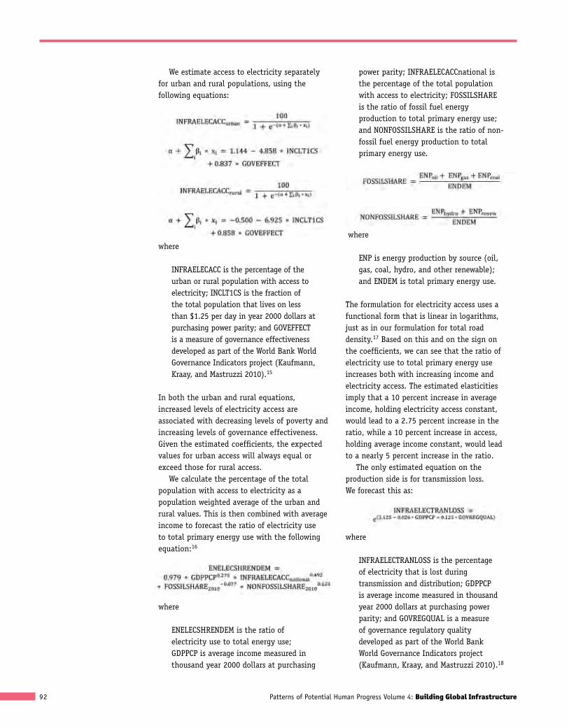
We estimate access to electricity separately for urban and rural populations, using the following equations:

where

INFRAELECACC is the percentage of the urban or rural population with access to electricity; INCLT1CS is the fraction of the total population that lives on less than $1.25 per day in year 2000 dollars at purchasing power parity; and GOVEFFECT is a measure of governance effectiveness developed as part of the World Bank World Governance Indicators project (Kaufmann, Kraay, and Mastruzzi 2010).15

In both the urban and rural equations, increased levels of electricity access are associated with decreasing levels of poverty and increasing levels of governance effectiveness. Given the estimated coefficients, the expected values for urban access will always equal or exceed those for rural access.

We calculate the percentage of the total population with access to electricity as a population weighted average of the urban and rural values. This is then combined with average income to forecast the ratio of electricity use to total primary energy use with the following equation:16

where

ENELECSHRENDEM is the ratio of electricity use to total energy use; GDPPCP is average income measured in thousand year 2000 dollars at purchasing

power parity; INFRAELECACCnational is the percentage of the total population with access to electricity; FOSSILSHARE is the ratio of fossil fuel energy production to total primary energy use; and NONFOSSILSHARE is the ratio of non-fossil fuel energy production to total primary energy use.

where

ENP is energy production by source (oil, gas, coal, hydro, and other renewable); and ENDEM is total primary energy use.

The formulation for electricity access uses a functional form that is linear in logarithms, just as in our formulation for total road density.17 Based on this and on the sign on the coefficients, we can see that the ratio of electricity use to total primary energy use increases both with increasing income and electricity access. The estimated elasticities imply that a 10 percent increase in average income, holding electricity access constant, would lead to a 2.75 percent increase in the ratio, while a 10 percent increase in access, holding average income constant, would lead to a nearly 5 percent increase in the ratio.

The only estimated equation on the production side is for transmission loss. We forecast this as:

where

INFRAELECTRANLOSS is the percentage of electricity that is lost during transmission and distribution; GDPPCP is average income measured in thousand year 2000 dollars at purchasing power parity; and GOVREGQUAL is a measure of governance regulatory quality developed as part of the World Bank World Governance Indicators project (Kaufmann, Kraay, and Mastruzzi 2010).18


This formulation implies that transmission loss falls with increasing income and improved governance regulatory quality.

Finally, although not shown in Figure 4.4, we recognize that a strong connection exists between the use of electricity and of solid fuels in the home. In general, as households move up the energy ladder, they increase their use of electricity and decrease their use of solid fuels (Holdren and Smith 2000), and we include a link in IFs from access to electricity to the use of solid fuels in the home. In previous versions of the model, where we did not estimate electricity access, we used income per capita, income distribution, and education as drivers in estimating the percentage of the population that primarily used solid fuels for heating and cooking (B. Hughes, Kuhn, et al. 2011: 98). We now have updated this formulation to include access to electricity as a key driver:

where

ENSOLFUEL is the percentage of the population using solid fuels as the primary fuel for heating and cooking; GDPPCP is average income measured in thousand year 2000 dollars at purchasing power parity; and INFRAELECACCnational is the percentage of the total population with access to electricity.

As incomes and access to electricity increase, the percentage of the population using solid fuels as the primary fuel for heating and cooking decreases.

Water and sanitationThe key access indicators we include for water and sanitation infrastructure are the percentages of the population with access to different levels of improved drinking water and sanitation and whose wastewater is collected and subsequently treated (see again Table 4.1). The physical quantities include the number of connections providing these services and the amount of land that is equipped for irrigation.

We originally introduced forecasts of access to improved sources of drinking water and sanitation into IFs in support of the previous volume in this series, Improving Global Health (B. Hughes, Kuhn, et al. 2011), because of the health risks associated with a lack of clean water and/or improved sanitation. For the purposes of the current volume, we have extended this portion of the model to include forecasts of the share of wastewater that is collected and then treated prior to being returned to the environment. In addition, we also added a component to forecast the area equipped for irrigation.

In Box 2.4 we introduced the concept of “ladders” for drinking water and sanitation. As countries develop, they ascend these ladders, gradually moving from a situation in which the majority of households have no access to improved sources of drinking water or sanitation to a point where most have piped connections delivering clean water and access to improved sanitation. We forecast the shares of the population in each of the water and sanitation ladder categories using

Figure 4.6 Modeling drinking water, sanitation, and wastewater infrastructure in IFs

Wastewatercollected

Access to improvedsource of drinking water

Averageincome

Poverty

Public healthexpenditures

Educationalattainment

Piped

Other improved access

No improved access

Access to improvedsanitation

Improved access

Shared access

Other unimproved access

Wastewatertreated

used in estimation along withexplanitory variables


Note: Some of the driving variables shown on the left affect the estimates of collected and treated wastewater directly, in addition to their effect through access to improved sanitation.


We forecast the shares of

population on each rung of the water

and sanitation ladders using

income, poverty levels, educational

attainment, and public health

expenditures as drivers.


average income, poverty levels (measured as the percentage of the population living on less than $1.25 per day), educational attainment (measured as the average number of years of formal education for adults over 25), and public health expenditures as explanatory variables (see Figure 4.6). These results then feed into the forecasts of the percentage of population with wastewater collection and wastewater treatment.

In forecasting the percentages of population with access to different levels of improved water and sanitation, we want to ensure that the estimated value in each category falls between 0 and 100 percent and that the values across the categories sum to 100 percent of the population. We accomplish this by using nominal logistic models (alternatively called

multinomial logit models). Our approach, in effect, estimates a set of coupled logistic equations that are then used to calculate the percentages (see Box 4.3).

The estimated coefficients for the two sets of nominal logistic models used to forecast access to sources of improved water and sanitation in IFs are shown in Table 4.3. While the underlying equations are reminiscent of those for the logistic equations described in Box 4.2, the interpretation of the coefficients is less straightforward since there are more than two categories. The general results show that countries move up the ladders as income, educational attainment, and government spending on health increase and poverty levels decrease. Furthermore, the formulations forecast lower levels of access to improved sanitation than drinking water, reflecting the situation in most countries (see again our discussion of the historical data in Chapter 2).

Although we use a separate equation for the percentage of the population connected to a wastewater collection system (see again Table 4.2), we do not allow that percentage to exceed the percentage of the population that has access to improved sanitation (see Box 4.4). We then forecast the share of the population whose collected wastewater is also treated; this is not allowed to exceed the percentage of the population connected to a wastewater collection system. These equations are as follows:

where

WATWASTE is the percentage of the population connected to a wastewater collection system; SANITATIONimp is the percentage of the population with access to improved sanitation; GDPPCP

Box 4.3 Estimating a nominal logistic model

In many situations, we wish to forecast the shares of population that fall into a finite set of categories. The logistic equation described in Box 4.2 is a special case, applicable when there are only two categories. When there are three or more categories, we can use a nominal logistic model for this purpose.

Assume that we have data showing the population divided into m categories, each representing a share p of the population, where the values of p sum to 1. Furthermore, assume that we wish to estimate a set of equations using a set of n explanatory variables.

We can estimate the values of p as:

where ai and bi,j are estimated coefficients and xj is the value of the explanatory variable.

The values for si can be shown to be the ratios of pi to pm, i.e., the ratios of the percentage of the population in category i to the percentage of the population in category m. The knowledge that the probabilities need to sum to 1 allows us to calculate one fewer equation than there are categories.

The resulting values of pm will all fall between 0 and 1 and sum to 1. These are then multiplied by 100 in order to obtain values that range between 0 and 100 and sum to 100.


is average income measured in thousand year 2000 dollars at purchasing power parity; POPURBANPCNT is the percentage of the population living in urban areas; and WATWASTETREAT is the percentage of the population whose wastewater is collected and subsequently treated.

Once again, this is a logistic equation. The percentage of the population whose wastewater is collected and subsequently treated increases with both average income and the percentage of the population with wastewater collection.

We use these access measures with our forecasts of population and average household sizes to then forecast the number of connections to water, sanitation, and wastewater treatment. Because of their different costs, we separately estimate the number of connections for each category of access to improved water and sanitation. We assume that the costs for connections to wastewater collection facilities are covered in the costs for improved sources of sanitation, so do not calculate a separate value for those connections. We do, however, include an additional cost for wastewater treatment.

There have been few forecasts of the area equipped for irrigation, and those that do exist tend to be based on very detailed analyses of specific situations. In a recent report from the United Nations Food and Agriculture Organization (FAO) looking out to the year 2050, Bruinsma (2011: 251) stated that the “projections of irrigation presented in this section are based on scattered information about existing irrigation expansion plans in different countries, potentials for expansion (including water availability) and the need to increase crop production.” Another report looking at global agriculture over the next

half century (Nelson et al. 2010), this one from the International Food Policy Research Institute, relies on exogenous assumptions of the growth in irrigated area. The authors do not specify the source of these assumptions, but some of the same authors (You et al. 2011) have reported on the irrigation potential for Africa, basing their conclusions on agronomic, hydrological, and economic factors.

Rather than attempt to replicate the level of detailed analysis of most previous studies, we forecast the area equipped for irrigation based on data from the FAO’s FAOSTAT and AQUASTAT databases on historical irrigation patterns and the area that could potentially be equipped for irrigation.19 These data are incomplete; for area equipped for irrigation, data are provided for 168 of the 183 countries included in IFs,

Box 4.4 The relationship between household sanitation connections and wastewater collection in historical data

We obtain data on access to improved drinking water and sanitation from the World Health Organization and United Nations Children’s Fund Joint Monitoring Programme (JMP) for Water Supply and Sanitation Data and Estimates; the data originate from national and international surveys and are available at http://www.wssinfo.org/data-estimates/table/.

For wastewater collection and treatment, we take data from the Environmental Indicators Database of the United Nations Statistics Division (UNSD), Department of Economic and Social Affairs. The data are derived from UNSD/UNEP Questionnaires on Environment Statistics, the Organisation for Economic Co-operation and Development (OECD) /Eurostat Questionnaire on the State of the Environment, and the OECD Environmental Data Compendium, and are available at http://unstats.un.org/unsd/environment/qindicators.htm.

Unfortunately, the JMP no longer provides information on household connections to piped sewer systems separately from other types of improved sanitation. In order to address this issue, we compared the data on wastewater collection against those on access to improved sanitation. Of the 181 country-year pairs with data on both indicators, there were only 14 cases (covering 7 countries) where the value for wastewater collection exceeded that for access to improved sanitation. This supports the assumption that the percentage of the population with wastewater collection should not exceed that with access to improved sanitation. For the initialization of the model, therefore, we adjust the data on wastewater collection to match that of access to improved sanitation when the former exceeds the latter.

Table 4.3 Estimated coefficients in the nominal logistic models for access to water and sanitation in IFs

estimated coefficients

Water intercept educational attainment average income Poverty Public health expenditures

s0 0.47200933 -0.4414453 -0.7033376 0.0253734 -0.1616335

s1 1.17414971 0.13867779 -1.1508133 0.01181508 -0.2769033

sanitation

s0 0.73081107 -0.6420051 -0.4497351 0.02170283 -0.1562885

s1 -2.1593291 0.22539909 -0.3555466 0.02823687 -0.1579957

Note: See Box 4.3 for a description of nominal logistic model. The three categories for access to improved water and sanitation are shown in Figure 4.6.Source: Authors’ estimates as represented in IFs Version 6.61.

We forecast the area equipped for irrigation based

on historical irrigation patterns and the area that could potentially be equipped for

irrigation.


and for the potentially irrigable area, data are provided for 117 of 183 countries. In our examination of these historical data, we found that a number of countries had already reached an apparent plateau in the amount of area equipped for irrigation that was often well below the potential indicated. For example, Argentina’s equipped area has stayed at a bit over 1.5 million hectares since the late 1970s, even though its potential is given as more than 6 million hectares. Why a country saturates below its ultimate potential is often unclear, but one obvious reason for some countries is that they receive enough rainfall to not warrant further irrigation.

As a result of this analysis, we assume that countries that appear already to have attained a level of saturation in their area equipped for irrigation will remain at their current level, even if this is below the potentially irrigable area. This applies to 67 countries. For the remaining countries, we extrapolate their recent growth in area equipped for irrigation, while not allowing them to exceed a specified level of saturation. If they do have a value for potentially irrigable area, we use this information and the current amount of equipped area to determine the saturation level. Specifically, the closer that a country’s current equipped area for irrigation is to its potentially irrigable area, the closer we set its saturation level to the latter value. For those countries without data on potentially irrigable area, we arbitrarily assume a saturation level that is slightly above their current equipped area, taking into account their total agricultural area, which is also provided by the FAO datasets.

The forecasted expected levels for additional areas equipped for irrigation and people with wastewater treated are passed to the IFs financial model directly. Physical connections for drinking water and sanitation, however, are generally attributed to households and not individuals, and our costs for them are per household. Therefore, in order to calculate those costs, we convert the forecasts of access to drinking water and sanitation from percentages of the population to numbers of people and then to numbers of households using country specific average numbers of persons per household, which are forecast elsewhere in the model.

Information and communication technologiesThe most dynamic changes in infrastructure in recent years have been in the area of information and communication technologies (ICT). The rate of change in this sector, both qualitative and quantitative, presents a serious challenge to forecasting for all but the shortest time horizons. However, the importance of the sector means that it cannot be ignored. With that in mind, we forecast four basic indicators of ICT infrastructure: fixed telephone lines, fixed broadband subscriptions, mobile telephone subscriptions, and mobile broadband subscriptions, all per 100 persons (see again Box 2.5 on measuring ICT infrastructure).

Our forecasts for the different forms of ICT infrastructure are driven in part by cross-sectional relationships with a variety of socioeconomic drivers. As Figure 4.7 shows, however, there are also interactions among the different forms of ICT. We describe how we handle these interactions after presenting the cross-sectional relationships for each of the ICT forms in IFs.

The cross-sectional relationships for each of the forms of ICT in IFs follow below:

Figure 4.7 Structure of estimated equations for ICT infrastructure in IFs

Regulatory quality

Mobile telephones Mobile broadband

Fixed telephones Fixed broadband

Urbanization

Population

GDP




where

INFRATELE is fixed telephone lines per 100 persons; ICTMOBIL is mobile phone subscriptions per 100 persons; ICTBROAD is fixed broadband subscriptions per 100 persons; ICTBROADMOBIL is mobile broadband subscriptions per 100 persons; GDPPCP is average income measured in thousand year 2000 dollars at purchasing power parity; and GOVREGQUAL is a measure of governance regulatory quality developed as part of the World Bank World Governance Indicators project (Kaufmann, Kraay, and Mastruzzi 2010).

For each technology, we found strong relationships indicating that usage levels (our proxies in this case for access) increase with rises in average income and governance regulatory quality; in the case of fixed broadband, we also found urbanization to be important, as one might expect for a technology whose installation is supported by population density.

As for the interactions between the different forms of ICT, we start with fixed telephone lines. Given the potential for substitution by mobile telephone lines, we assume that the demand for fixed telephone lines will decline as mobile usage increases. Already we see this happening in the data, especially, but not exclusively, in high-income countries. Our analysis of the historical data indicates a level of approximately 30 mobile telephone subscriptions per 100 persons as the point at which fixed-line telephone decline begins, so we build this into our forecasts algorithmically. We do not expect that fixed telephone line usage will completely disappear. Rather, we assume arbitrarily that it will settle at a low level; this is set by default to 2.5 lines per 100 persons, but model users can change it. Furthermore, we also assume that: (1) mobile broadband subscriptions will never exceed mobile telephone subscriptions; and (2) any decline in fixed telephone lines will boost the growth in fixed broadband because countries that have existing investments in fixed-line infrastructure are able to leverage

Figure 4.8 Changing relationship between mobile telephone subscriptions and average income over three points in time: 2000, 2005, and 2010

Mobile telephone subscriptionsper 100 persons

200

0

40

20

60

80

100

120

180

140

160

0 806040 705020 3010

GDP per capita at PPP (2000$)

2000 2005 2010

Source: IFs Version 6.61 using data from the World Bank World Development Indicators available at http://data.worldbank.org/data-catalog/world-development-indicators and the International Telecommunication Union World Telecommunication/ICT Indicators database available at http://www.itu.int/ITU-D/ict/statistics/.

For ICT, our forecasts of usage levels (a proxy for access rates) are based on income,

governance regulatory quality, and in the case of fixed broadband, urbanization.


these networks to provide broadband access with rather modest investments.

The cross-sectional relationships with income do not remain static across time for mobile phones, fixed broadband, and mobile broadband. Figure 4.8 shows this for mobile telephone subscriptions. The individual points reflect historical data for country access rates for the years 2000, 2005, and 2010. The lines are logarithmic curves fit through these data. The upward shift over time reflects advances in information and communication technologies that are making ICT cheaper and more accessible around the world. These advances are, in turn, driven by various systemic factors ranging from product and process innovation to network effects.20

In order to capture the effect of this rapid change in our forecasts of future access, we combine the use of the cross-sectional function with an algorithmic approach that simulates the upward shift of the curves for mobile phones, fixed broadband, and mobile broadband. The algorithmic element assumes a standard technology diffusion process in which the growth in penetration rate associated with the technological shift rises from a low annual percentage point increase at low levels of penetration to a maximum at the middle of the range (the inflection point) and falls again as saturation is approached (see Figure 4.9).21 For each of the three technologies, we have looked at historical patterns to estimate the minimum

and maximum growth rates, expressed as annual percentage points of absolute change. These are summarized in Table 4.4 and can be modified by the user.

The choice of saturation levels is obviously quite important. Data from the International Telecommunications Union show penetration rates for mobile phones that exceed 100 subscriptions per 100 persons (e.g., approaching 200 in Hong Kong). At the same time, some countries (e.g., Denmark) seem to be reaching a saturation level for fixed broadband well below 100 subscriptions per 100 persons. Uncertainty remains over the proper level of saturation to assume for these subscriptions, and therefore, different researchers use different values. Specifically, we define saturation as 50 subscriptions per 100 persons for fixed broadband and 150 subscriptions per 100 persons for both mobile technologies.22 In addition, we assume that mobile broadband penetration cannot exceed mobile phone penetration.

As with the other forms of infrastructure, prior to calculating financial forecasts, we convert the forecasted demand for the four indicators of ICT infrastructure, which are given in terms of per 100 persons, to actual numbers of subscriptions. In this case, this is done in a quite straightforward fashion by multiplying by total population divided by 100.

Translating the expected levels of infrastructure into financial requirementsIn estimating the financial requirements to achieve the expected levels of infrastructure, we adopt the approach introduced by Fay (2001) and Fay and Yepes (2003) described earlier. Recall that in this approach, there are two components to the financial requirements for each type of infrastructure each year. First

Figure 4.9 Determining the technological shift factor in IFs as a function of level of ICT access

Maximumgrowth rate

Minimumgrowth rate

Inflection point

Level of access

Saturation level

Tech

nolo

gica

l shi

ft fa

ctor

High accessLow access


We estimate infrastructure

spending needs both for new

construction and for maintenance and

renewal of existing infrastructure.

Table 4.4 Minimum and maximum annual increases in ICT infrastructure in percentage points

Minimum Maximum

Mobile telephones 1.0 3.0

Fixed broadband 1.0 2.5

Mobile broadband 1.0 8.0

Note: The minimum increases effectively drop to 0 as penetration reaches saturation.



there is the cost of maintenance/renewal of existing infrastructure. This is determined as a percentage of the “dollar value” of the existing infrastructure, where the dollar value is given as the amount of infrastructure at the start of the year multiplied by the infrastructure’s unit cost. Second, there is the cost of new construction. This is calculated as the expected net change in the amount of physical infrastructure over the year multiplied by the same unit cost.

The annual maintenance/renewal percentages and unit costs are obviously key assumptions in the estimates of the financial requirements. Earlier we noted that there are a number of questions related to modeling unit costs for each type of infrastructure. Should they differ based on a country’s political, economic, or geographic circumstances? Should they differ depending on the level of existing infrastructure? Should they differ depending on whether the investments are made by the public or private sector?

With a few exceptions noted in our discussion of other studies earlier in this chapter, most previous studies have held

unit costs constant across countries, levels of infrastructure, and time. For this reason, as well as the lack of data needed to specify variable costs and the complications this lack would introduce to the analysis, we also assume temporally fixed and geographically universal unit costs by infrastructure type (one cost per infrastructure type).

The unit costs we use, expressed in constant dollars at year 2000 market exchange rates, are summarized in the third column of Table 4.5. The values reflect our judgment, informed by the previous studies discussed earlier in this chapter and summarized in this chapter’s Appendix 4A.

The fourth column in Table 4.5 presents our Base Case assumptions for the average lifetimes of the various types of infrastructure, and the fifth column translates these into annual maintenance/renewal percentages. The average lifetimes were determined in the same way as the unit costs, and are also held constant across countries and time for similar reasons. The annual maintenance/renewal percentages are determined using the average lifetimes and assuming a simple exponential decay.23

We separate total funding

requirements into public and private

components.

Table 4.5 Unit costs, lifetimes, and public shares of funding by infrastructure type in IFs

infrastructure type unit

unit cost 2000$ per

unit

average lifetime(years)

equivalent annual recurrent cost(Percent of stock value)

Public share (Percent)

Paved roads Per kilometer 425,000 50 1.39 80

Unpaved roads Per kilometer 40,000 10 6.93 80

Electricity connection – rural Per connection 1,750 40 1.73 80

Electricity connection – urban Per connection 850 40 1.73 80

Electricity generation capacity Per kilowatt of added capacity 1,900 40 1.73 80

Irrigation Per hectare 5,000 40 1.73 80

Improved water connection – piped Per household connection 500 40 1.73 80

Improved water connection – other improved Per person 45 20 3.47 80

Sanitation connection – improved Per household connection 750 40 1.73 80

Sanitation connection – shared Per person 95 20 3.47 80

Wastewater treatment Per person 120 30 2.31 80

Fixed-line telephone Per line 200 12.5 5.55 20

Fixed-line broadband Per subscription 250 12.5 5.55 10

Mobile telephone Per subscription 125 12.5 5.55 5

Mobile broadband Per subscription 150 12.5 5.55 5

Note: Values are based on prior studies and authors’ judgment. Unit costs are expressed in year 2000 dollars at market exchange rates (MER). Costs for electricity generation capacity include transmission and distribution. Unit costs for some countries are adjusted by a factor determined in the first year in order to balance government expenditures with historical data; these gradually converge to the values shown in the table.



Finally, given that in the real world funding for infrastructure comes from both public and private sources, we wanted to separate the funding requirements into public and private components. More specifically for our purposes, the balancing of the financial requirements with the available resources included in IFs and described in the next section only considers the public sector. We assume a specific share of public and private funding for each type of infrastructure. This, in effect, implies that public spending on infrastructure leverages a certain amount of private spending. Again, these shares differ by type of infrastructure (note especially the far greater share of private spending associated with ICT than with the other core infrastructure types), but are constant across countries and time. The final column of Table 4.5 summarizes our assumptions about these shares. Our choices for these shares were based on limited historical data and our own judgment.

The IFs user can modify the assumptions on unit costs, infrastructure lifetimes, and public shares. In Chapters 5 and 6, we explore the sensitivity of many of our key results to variations in a number of these assumptions.

Balancing the financial requirements with available resourcesThere is no guarantee that the requirements for infrastructure funds will match those made available. In determining whether this is the case, we focus on the public spending for infrastructure. In IFs, government domestic revenues and net foreign aid

are allocated between transfers (pensions and other social payments) and direct government spending. The latter is divided among broad categories—defense, education, health, research and development, basic infrastructure (those types represented explicitly in IFs), “other” infrastructure (see Box 4.5), and a residual category of other government spending. It is through this process of allocating government revenues that the amount of public funding for infrastructure ultimately is determined. The IFs model does allow some imbalance between revenues and total expenditures year to year, but neither debt nor surpluses can accumulate indefinitely; as their percentages of GDP change, signals adjust revenues and expenditures over time.

Once the total funds available for direct government spending are determined, they are compared to the total funding requirements across the various categories.24 In the case of demand-supply mismatches, the default rule is to allocate the subtractions from, or additions to, specific categories based on their relative share of total funding requirements. It is also possible to prioritize funding for two specific categories—education and infrastructure—in the case of funding shortfalls.25 In this case, the user-defined portion of the desired funding for the prioritized category or categories is funded first, up to the level of total government spending. Any remaining available government spending is then allocated proportionately to the remaining (unprioritized) portion of desired funding for these and the other categories.

Determining the forecasted levels of physical infrastructure actually attainedOnce the total amount of public funding for infrastructure is determined, we can forecast the levels of infrastructure that will be attained. If there is a match between the estimated funding requirements and the estimated funding available, the process is fairly straightforward: the level of infrastructure constructed and maintained will be equal to the expected level of infrastructure. In the case where there is a demand-supply mismatch, the forecasting becomes more complicated.

In the case of a budget shortfall, we make three simplifying assumptions. First, we

Box 4.5 Public spending on “other” infrastructure

Our focus in this volume is on what we have called “core” infrastructure—roads, electricity generation, improved water and sanitation, and ICT—and on access to it. Although we do not represent other forms of infrastructure explicitly, we do estimate spending on them in order to avoid almost certainly underrepresenting the total demand for infrastructure. Based on historical data, we estimate that spending on “other” infrastructure gradually increases with average income from around 1.8 percent of GDP to 2.2 percent of GDP. Therefore, our forecasts also include a demand for funding for “other” infrastructure that is purely a function of GDP per capita.

There is no guarantee that

requirements for infrastructure funds

will match those made available; in the case of a

funding shortfall, the forecasted levels of infrastructure will

be constrained.


assume that all forms of infrastructure are affected equally; specifically, each receives the same proportionate cut in the amount of public funding received. Second, with the exception of ICT infrastructure (fixed and mobile telephones and broadband), we assume that the amount of private funding is reduced by the same proportion. This is based on our premise, stated earlier, that public funding for infrastructure leverages private spending, so less public funding also means less private spending. We make the exception for ICT because this is a less-tenable assumption for that sector given the degree to which private spending historically has driven ICT development. Specifically, private funding for ICT is not reduced even in the case of a reduction of public funding. Third, we assume that the reductions in funding affect spending on both maintenance and new construction equally.26 The net result is that there will be less new construction of infrastructure than desired, as well as less maintenance of existing infrastructure. This can lead to an absolute decline in some forms of infrastructure when the new construction is not enough to make up for the amount of infrastructure lost due to inadequate maintenance.

When there is a budget surplus, the extra funds go to additional new construction because the maintenance/renewal requirements are already covered. The default is for the surplus to be spread across the different forms of infrastructure based on: (1) their initial share in public infrastructure funding; and (2) the distance from universal access. In some cases, however, the additional funds would result in illogical levels of access, such as more than 100 percent of the population having access to electricity. In such instances, the excess funds are redistributed to other forms of infrastructure. Private funding is not affected by increases in public funding from “surplus funds.”

Finally, we recognize that, much like Rome, infrastructure is not built in a day. Nor is it built in a year. The appearance of new infrastructure generally reflects investment that has occurred over a number of years and, especially in the case of major water projects, even decades. The foundational patterns of our forecasts do not explicitly represent such delays, however, because

for aggregate infrastructure categories in countries as a whole, it is reasonable to smooth both spending and construction completion patterns. In some cases, however, including scenario analyses like those of Chapter 6 in which infrastructure-related targets are pursued, we do forecast dramatic increases in funds being made available for infrastructure from one year to the next, reflecting a ramping up of infrastructure development. In these cases, we hold back a portion of the new funds being made available and gradually release the money over a number of years. In this way, we approximate the time lags in the conversion of spending on infrastructure to its actual attainment.

Estimating the economic, social, and environmental impacts of physical infrastructureWe described a number of the social, economic, and environmental impacts of infrastructure in Chapter 3. We divided these into impacts on economic growth, income distribution, health, education, governance, and the environment. Given the limited empirical support for many of these linkages and, thus, a high level of uncertainty about whether and how to represent them, we have limited our inclusion of direct links from infrastructure to the links from infrastructure to economic growth and health.27 Important indirect linkages supplement the direct linkages that we describe here. For example, the forward linkages from economic growth to environmental impact (via paths such as increased energy use and food demand) and from improved health to demographic change are present in the current model. In fact, the indirect linkages via both of these paths are pervasive across the model.

Impacts on productivity and economic growthWe estimate the impact of infrastructure on economic growth through its effect on multifactor productivity. Most economic models relate aggregate growth to changes in factors of production, typically capital (K) and labor (L), and an additional component, which is variously called the Solow residual, the technological change parameter, total factor productivity (TFP) or multifactor productivity (MFP); here we use the MFP label. Analyses have long shown that MFP

While new infrastructure

generally reflects investment that

has occurred over a number of years or even decades,

our forecasts do not explicitly represent

such delays.


can be quite large (Solow 1956; 1957).28 Within IFs, we treat MFP as an endogenous variable that human capital, social capital, physical capital, and knowledge capital influence (B. Hughes 2007). Infrastructure is a key component of physical capital, along with natural resources. The impact of the latter is represented through the effect of energy prices on MFP.

In estimating the impact of infrastructure on MFP, we build on the insights of the studies reviewed in Chapter 3. First, we relate the impact to measures of physical infrastructure and not to measures of infrastructure spending. Second, because of the interaction effects across infrastructure types, we do not attempt to estimate the impact of individual forms of infrastructure but rather estimate the impact as a function of a composite index of infrastructure. Due to the very different historical and expected growth patterns of more traditional infrastructure—transportation, energy, and water—vis-à-vis ICT, however, we create a separate index for ICT and link it to MFP in a different way.

For the more traditional forms of infrastructure, we construct our composite index following the approach that Calderón and Servén (2010a) presented. We use the indicators shown in Table 4.6, which include a mix of measures of infrastructure quantity and quality (such as

paved roads). A first step in index construction is to scale each measure by a meaningful factor, for example, population or land area; it obviously makes more sense to compare countries in terms of, for example, roads per person than total roads. Second, we normalize and standardize each indicator by taking the logarithm of the scaled measure, calculating the difference between this value and the mean value across countries, and then dividing the result by the standard deviation of these values across countries.29 The mean value and standard deviation for each indicator are based on the country-level data for 2010, the base year of our model. A negative (positive) value of a transformed indicator implies that a country ranks below (above) the average country in 2010 for that indicator. For example, a country with a negative value for total roads per 1,000 persons in our forecast for 2030 would have fewer roads per person than the average country in 2010.

We then take a simple average of the resulting values for each transformed indicator in a category to calculate the index for that category.30 The Transportation Index, for example, is calculated as one-quarter of the sum of the transformed values for total roads per 1,000 persons, total roads per 1,000 hectares, the Rural Access Index, and the percentage of roads paved. Finally, we calculate a simple average of the Transportation, Energy, and Water indices to produce the overall Traditional Infrastructure Index.31 As with the transformed values of the individual indicators, the value of the overall index can be positive or negative, indicating how a country compares against the average country in 2010. The values of the overall index range from approximately -2 (Chad and Togo) to +1 (Sweden) in 2010. There is also a natural ceiling of approximately +1.2, as each of the components of the index has a clear upper limit (e.g., the access measures that cannot exceed 100 percent) or shows a clear pattern of saturation.

We use the overall Traditional Infrastructure Index to calculate the impact of traditional infrastructure on MFP in the same way as we do for most factors that influence MFP. As described by B. Hughes (2007: 15–16), we do this by comparing the value of the index for a country to a benchmark function that indicates what value we would expect to see

The impact of infrastructure on multifactor productivity in

IFs is a function of a composite

index of physical infrastructure.

Table 4.6 Components of infrastructure indices in IFs

traditional infrastructure index

Transportation Total roads per 1,000 persons

Total roads per 1,000 hectares

Rural Access Index

Percentage of roads paved

Energy Electrical generation capacity per capita

Percentage of population with access to electricity (total)

Transmission loss percent

Ratio of electricity use to total primary energy use

Water Percentage of population with access to improved water

Percentage of population with access to improved sanitation

Percentage of population with wastewater treatment

Modern infrastructure index

ICT Mobile phone subscription rate

Fixed broadband subscription rate

Mobile broadband subscription rate

Source: IFs version 6.61.


for a country given its current level of GDP per capita (see Figure 4.10). A country whose index falls above (below) the benchmark value receives a boost to (reduction from) its MFP. For example, Gabon and Latvia have similar levels of GDP per capita in 2010, but Latvia’s Traditional Infrastructure Index falls well above the benchmark line, while Gabon’s falls well below. Thus, the former will receive a boost to its MFP due to traditional infrastructure, while the latter will receive a reduction. The size of the boost or reduction depends on the distance from the benchmark value and a factor relating this distance to productivity. Calderón and Servén (2010a: i35) presented a value of 2.193 percentage points as their estimate of the increase in the annual average growth rate of GDP per capita associated with an increase of 1 unit in their index. Based on this, we use a default value of 2 percentage points for the effect of traditional infrastructure on MFP. Specifically, if the value of the Traditional Infrastructure Index for a country is a full point above its expected value in a given year, it would receive a 2 percentage point boost to its MFP, which roughly translates into the same increase in growth in GDP per capita, over the coming year.32 The model user can change this value, allowing for exploration of the sensitivity of model results to the traditional infrastructure parameter.

When considering the impact of ICT infrastructure on MFP, however, this same structure runs into problems. Recall that our formulation for forecasting ICT infrastructure includes a technology shift factor. Therefore, any relationship between GDP per capita and the expected level of ICT would not remain stable over time; for example, a country with a GDP per capita of $5,000 in 2015 would be expected to have more ICT infrastructure than a country with a GDP per capita of $5,000 in 2010.

We therefore associate the growth contribution from ICT advances with annual changes in the ICT Index (see again Table 4.6), rather than with the level of the index as we do for traditional infrastructure. The ICT Index is an average of access rates for different kinds of ICT.33 We multiply the annual unit change in the ICT Index by a factor representing the increase in MFP resulting from a unit change. Qiang, Rossotto and Kimura (2009:

45) estimated that each 10 percent increase in broadband penetration in developing countries increased the growth rate of per capita GDP by 1.38 percentage points (by 1.21 percentage points for developed countries) during the 1980 to 2006 period.34 We arbitrarily reduce the impact by using a default and user-changeable parameter of 0.8 because our index is a mixture of several types of ICT infrastructures, not all of which might have as strong an impact on economic productivity as does broadband. Thus, a 10 point increase in the value of the ICT index would result in a 0.8 addition to MFP, or an approximate increase of 0.8 percent in GDP per capita.

There is one obviously questionable implication of this approach. When a country reaches saturation in the ICT Index, it will no longer receive a productivity boost from ICT. Given the current rapid increase in mobile telephones and mobile broadband that together make up two-thirds of the ICT Index, we see in most scenarios a near-term boost to MFP from ICT in much of the world, followed by little or no contribution later in the horizon. Our uncertainty with respect to appropriate treatment of the longer-term contribution of ICT points to one of the limitations of trying to forecast rapidly changing technologies.

Figure 4.10 IFs Traditional Infrastructure Index vs. GDP per capita: Benchmark function 2010

Actual IndexTraditional Infrastructure Index

1.0

–2.5

–1.5

–2.0

–1.0

–0.5

0.0

0.5

0 806040 705020 3010

GDP per capita at PPP (2000$)

Expected Index

Note: The benchmark function is based on data from 2010, the base year of the model.



Impacts on healthChapter 3 reviewed many ways in which infrastructure can affect human health. We have chosen to limit our inclusion of these effects to a small set, specifically the impact of (1) unsafe water, sanitation, and hygiene directly on diarrheal diseases, and indirectly on diseases related to undernutrition; and (2) indoor air pollution on respiratory infections, such as pneumonia, and respiratory diseases, such as chronic obstructive pulmonary disease. These health outcomes are influenced directly by infrastructure via our measures of access to improved sources of drinking water and sanitation and the use of solid fuels in the home. These measures serve as proxies for the environmental health risks linked to infrastructure in IFs. We explored these effects in a previous volume in this series, Improving Global Health (B. Hughes, Kuhn, et al. 2011: 95–100), and have some confidence in the reasonableness of our results.

Since B. Hughes, Kuhn, et al. (2011: 44–47) presented in detail our approach for estimating the impact of these health risks and the approach has not fundamentally changed,35 we provide only a brief overview here. In general, we compare the forecasted values of these infrastructure indicators to values that we would anticipate based only on income and educational attainment (distal drivers). If the estimated and expected values differ, we adjust the levels of mortality and morbidity for the associated diseases forecasted based only on the distal drivers. For example, if the levels of access to improved sources of water and sanitation are higher than expected, we reduce the mortality rate from diarrheal diseases. The amount by which the mortality rate is reduced is based on the analysis presented in the Comparative Risk Analysis work of the World Health Organization (Ezzati et al. 2004). This general approach, comparing forecasted values with expected ones and translating the difference into impact in a forward linkage, is fundamentally similar to the method described earlier in this chapter for linking infrastructure development and economic productivity.

ConclusionModeling the future of infrastructure presents many challenges. A comprehensive infrastructure forecasting system would include a representation not only of the expected levels of infrastructure, but also the ability for those expected levels to be met, and the socioeconomic and environmental impacts of building and maintaining infrastructure or of failure to do so. As we have seen, there are both theoretical and empirical (e.g., lack of good historical data) hurdles to clear in creating such a forecasting capability.

In fact, we are not aware of any previous attempt to model a fully integrated infrastructure system. Most work has focused solely on the expected levels of future infrastructure, often with some attention to the funding potentially needed to meet those expected levels, so as to alert policy makers to that need. Previous efforts do, however, help us understand some of the needed foundational elements. We have built on these efforts to implement a dynamic, integrated infrastructure model within the broader IFs system. This will allow us to explore more completely not only the likely, but also the more desirable, future patterns of infrastructure development and their two-way interaction with broader socioeconomic development.

We recognize that any model, ours included, simplifies reality. We do not cover all forms of infrastructure. In addition, our representations of the expected developmental pattern for infrastructure, the budgeting process, the actual construction and maintenance of infrastructure, and the forward linkages of infrastructure, are all subject to errors.

The role of infrastructure in development processes is too important for us to let the challenges deflect us from seeking to better understand its future, however. We therefore will move ahead in the next chapter to present a Base Case scenario of the availability of, and access to, infrastructure, as well as the associated costs. Chapter 6 will then consider the costs and benefits of more aggressive pursuit of infrastructure development than we will see in the Base Case.

IFs explicitly models the health impacts of unsafe water, sanitation, and hygiene, and also of indoor air

pollution.


1 For an introduction to the character and use of the model, see B. Hughes and Hillebrand 2006.

2 More technically, the model structure is recursive; that is, it computes equations sequentially in each time-step without simultaneous solution. It combines features of systems dynamics (notably, the accounting structures with careful attention to both flows and stocks) and econometrics (with estimated parameters specifying the dynamic behavior of the agent classes).

3 Bhattacharyay takes two approaches to forecasting expected levels and costs: a “top-down” approach that estimates national-level infrastructure based on population, GDP, and other characteristics; and a “bottom-up” approach for regional or international projects. His top-down approach follows a similar methodology to the other studies cited here.

4 An earlier version of WEM provided the electricity generation capacity forecasts for the Organisation for Economic Co-operation and Development Infrastructure to 2030 study (Morgan 2006).

5 GISMO, in fact, directly uses the basic IFs economic model (Hilderink et al. 2008: 73–83).

6 G. Hughes, Chinowsky, and Strzepek (2009) used separate percentages to calculate replacement and maintenance.

7 These differences are much too large to be explained by the use of different base years (2005 for G. Hughes, Chinowsky, and Strzepek [2009] and 2009 for Kohli and Basil [2011]). In some cases, they are explained by inter-regional price differences and changes in technology; for example, ICT infrastructure costs have gone down substantially over time.

8 Kohli, Szyf, and Arnold (2012: 112) describe an update to the infrastructure model presented in Kohli and Basil 2011 in which they incorporate regional price level differences.

9 In developing this volume, we made significant changes in our approach to forecasting ICT. We also recognized the need to further develop the energy model within IFs, which remains to be completed. This raised questions about the relationships between ICT and energy efficiency and the relative costs of renewable energy. Consequently, those relationships have been removed for the time being.

10 Further details can be found in the IFs help system and in additional technical documentation on the infrastructure model, both of which are available at http://www.ifs.du.edu.

11 Not all countries have data for all indicators included in the model in the base year. IFs includes a preprocessor that uses a series of algorithms that draw on historical data for previous years, the estimated equations, and other factors to initialize these missing data.

12 Standard data sources, such as the World Bank World Development Indicators, provide financial variables at market exchange rates (MER), and therefore we use MER for economic accounting systems (including national revenues and expenditures) throughout the Ifs system. Causal relationships built across countries benefit, however, from the more accurate comparison of countries inherent in representations at purchasing power parity (PPP), and therefore we use PPP

in estimations and forecasting of such causal relationships.

13 Ingram and Liu (1999: 17) found the elasticity between income density and total road density to be about 0.7. Thus a 10 percent increase in income density would yield a 7 percent increase in road density. Glover and Simon (1975: 464) find roughly the same elasticity of 0.7 between population density and total roads.

14 Total primary energy use is forecast elsewhere in IFs as the product of total GDP and energy use per unit GDP. Energy use per unit GDP decreases as a function of increasing per capita income, using a relationship derived from historical patterns. As with many other equations within IFs, the forecasts also include country-specific shift factors estimated from the differences between predicted and actual values in the base year.

15 The World Bank governance effectiveness measure ranges from -2.5 to +2.5, with a higher value indicating greater effectiveness. For our estimation and forecasts, we shift the scale to range from 0–5.

16 In estimating this ratio, we found that a significant fraction of the variation not explained by average income or electricity access was related to a country’s energy production relative to its consumption, but that the direction of the effect depended on the type of energy produced. Large producers of fossil fuels (e.g., many Middle Eastern countries) use much less electricity than expected. Meanwhile, large producers of hydroelectric (e.g., Tajikistan) or other forms of renewable energy (e.g., Iceland), use much more electricity than expected. Given the extreme uncertainty in the expected changes in the shares of renewable and nonrenewable energy production in the future, we keep the fossil and non-fossil fuel shares of energy production constant over time.

17 It is possible to argue that we should use a logistic function here as the ratio of electricity use to total energy use must necessarily fall between 0 and 1. Because we know that there must be some energy loss in the transformation from primary energy to electricity, however, the maximum value for the ratio is some unknown value less than one. This unknown value makes the logistic formulation difficult to use. Fortunately, the logarithmic form behaves well, staying below 1 for even extreme values of the explanatory variables.

18 The World Bank governance regulatory quality measure ranges from -2.5 to +2.5, with a higher value being better. For our estimation and forecasts, we shift this scale to range from 0–5.

19 These are available at http://faostat3.fao.org/home/index/html and http://www.fao.org/nr/water/aquastat/main/index.stm, respectively. The area potentially equipped comes from country and regional studies that use inconsistent methods and consider different factors.

20 Kalba (2008) discusses this in great detail.

21 This would result in a standard S-shaped growth pattern over time in the absence of the growth expected from the changes in the explanatory variables in the cross-sectional functions.

22 For an example of a different assumption, see Kohli and Basil (2011: 78). They assume a saturation

level of 250 mobile phone subscriptions per 100 persons in their forecasts.

23 This means that the annual maintenance/renewal percentage is calculated as the natural logarithm of 2 divided by the average lifetime.

24 The government budgeting submodel, representing all revenue and expenditure streams and their balancing over time, is part of the larger dynamic social accounting matrix structure of IFs (for more information, see B. Hughes and Hossain 2003).

25 Sixty percent of the desired education funding is protected in the IFs Base Case. While infrastructure funding is not protected in the Base Case, it can be protected in user-defined scenarios, and we do so in some of the explorations in Chapter 6.

26 A reviewer of a draft manuscript of this volume pointed out that infrastructure maintenance (other than wages and salaries of public sector workers) gets a much lower priority than new construction in most developing countries. Changing our assumption that expenditure reductions impact new construction and maintenance equally would change the breakdown between spending on new constructions and maintenance in our model, but would not affect the overall amount of infrastructure. This is because we define “maintenance” as being equivalent to renewal, and use the same unit cost (pro-rated over expected lifetimes for maintenance) as the basis for both new construction and maintenance. Furthermore, since we do not deal explicitly with the vintage and quality of infrastructure, other model results would not be affected.

27 In the development of IFs, we often include relationships that are quite obviously existent and important even when we do not have strong bases for specific formulations and parameters, because we believe that an explicit and rough estimate of such relationships is better than an implicit and clearly wrong omission of them. We expect over time to extend our infrastructure modeling to incorporate directly some of the relationships we have omitted here, including, for instance, the effects of rural roads on increasing educational enrollment rates and on reducing spoilage of agricultural products that otherwise cannot reach markets.

28 The estimate by Solow (1957: 320) that technical change accounted for 87.5 percent of growth in economic output per worker-hour in the United States from 1909–1949 focused the minds of everyone interested in growth on the Solow residual. From growth accounting estimates in four panels of countries, Barro and Sala-i-Martin (1999: 380–381) reported unweighted average estimates of TFP that were considerably lower, but still impressive: 40.7 percent for seven OECD countries from 1947–1973 (33.6 percent for the U.S.); 34.8 percent for the G-7 countries from 1960–1990 (13.2 percent for the U.S.); 24.3 percent for seven Latin American countries from 1940–1980; and 14.2 percent for four East Asian countries from 1966–1990. Even though it is generally understood that the productivity share of growth is lower in less developed countries than in OECD countries, it is clearly sufficiently high and variable to be an important factor in growth forecasting and development analysis.


29 Standardizing the data by dividing the difference from the mean by the standard deviation insures that changing the units of measures (e.g., from kilometers to miles) does not affect the results and creates comparability across measures.

30 This is slightly different from Calderón and Servén (2010a), who used the coefficients of the first principal component of their infrastructure variables as the weights in their index. Their weights were roughly similar to ours in any case.

31 One could imagine the use of a geometric mean for combination of individual indicators so as to represent some of the interaction effects across measures (Fleming and Wallace 1986); the use of logarithms in the transformation process for each indicator helps avoid the possibility that increases to

extreme values on one infrastructure measure might be interpreted as comparably important as increases at more modest levels on a second measure.

32 The model represents interaction effects across the various contributions to MFP. Thus, in the absence of somewhat parallel advance in the MFP human capital and social capital terms, a very large increase from infrastructure development in the MFP physical capital term will have less impact on economic growth than such an increase in the context of more balanced development.

33 The subscriptions for mobile phones and mobile broadband are multiplied by 2/3 so that they range from 0 to 100 prior to taking the average of these and fixed broadband subscriptions.

34 Qiang, Rossotto and Kimura (2009) do not appear to take into account any delays in broadband’s impact or changes in that impact over time, and neither do we.

35 While our approach has not fundamentally changed, we have updated it by: (1) using more detailed data from the WHO/UNICEF Joint Monitoring Programme; (2) reestimating the equations; and (3) renaming the water and sanitation categories to match similar changes recently made by JMP (see WHO and UNICEF Joint Monitoring Programme for Water Supply and Sanitation 2012).


Appendix 4A: Unit Cost Assumptions Used by Other Studies for Infrastructure Construction and MaintenanceAs noted in the body of this chapter, the unit costs and annual maintenance/renewal rates assumed in previous studies that forecast infrastructure spending requirements can differ markedly. In this Appendix, we compile the various estimates we have found (listed by date of publication). Since the purpose of this review was to provide us with ballpark estimates, we have not tried to fully reconcile the differences across the studies. With the exception of G. Hughes, Chinowsky, and Strzepek, who provided us with detailed spreadsheets, the values in the tables are taken directly from the published

papers cited. We encourage the interested reader to look at the original studies for further details on these assumptions.

Note that G. Hughes, Chinowsky, and Strzepek multiplied their unit costs by a country-specific building cost factor that ranged from 0.8 to 1.1; these are not shown in the tables. Also, while some studies did use different unit costs for different regions or over time for some forms of infrastructure, in most cases a single unit cost was provided for each form of infrastructure.

Roads

Table 4A.1 Unit costs used by other studies for building and maintaining paved roads

study regional coverage unit of measurecost per unit of new construction

annual recurrent cost per unit(Percent of stock value)

Fay (2001: 11) Latin America 1995$ per kilometer 200,000 Not included

Fay and Yepes (2003: 10) Global 1995$ per kilometer 410,000 2

Yepes (2005: no page number) East Asia and Pacific $ per kilometer 417,995 2

Chatterton and Puerto (2006: 7, 9–10) South Asia $ per kilometer 425,000 2

Yepes (2008: 7, 10, 11, 15) Global 2005$ per kilometer 410,000 4 to 5

G. Hughes, Chinowsky, and Strzepek (values used in 2009 study; spreadsheet provided by authors)

Global 2005$ at PPP per kilometer

600,000 2

Asian Development Bank Institute (2009: 27–28) for new construction costs; Bhattacharyay (2010: 10) for annual recurrent costs

Central Asia, East Asia and Pacific, Southeast Asia

2008$ per kilometer 425,000 2

Kohli and Basil (2011: 96) Latin America 2009$ per kilometer 895,000 2

Note: All values are in constant U.S. dollars, with currency year and whether based on purchasing power parity (PPP) or market exchange rates (MER) shown when specifically identified in the original source. Unit costs for roads are per one kilometer of two-lane road. In general, the unit costs for roads (both paved and unpaved) stem from the Road Costs Knowledge System, a database of country-specific roadwork costs and related data gathered and disseminated annually by the World Bank and available at http://go.worldbank.org/ZF1I4CJNX0. Most studies assume a single best-practice cost regardless of country or region. Maintenance costs for roads reflect only general upkeep and do not include costs associated with rehabilitation.


Table 4A.2 Unit costs used by other studies for building and maintaining unpaved roads



Yepes (2008: 7, 10, 11, 15) Global 2005$ per kilometer 50,000 7.3


Global 2005$ at PPP per kilometer

40,000 10

Note: See note accompanying Table 4A.1.

Electricity generation

Table 4A.3 Unit costs used by other studies for building and maintaining electricity generation capacity



Fay (2001: 11) Latin America 1995$ per kilowatt 1,500 Not included

Fay and Yepes (2003: 10) Global 1995$ per kilowatt 1,900 2

Yepes (2005: no page number) East Asia and Pacific $ per kilowatt 1,900 2

Chatterton and Puerto (2006: 7, 9–10) South Asia $ per kilowatt 1,900 3

Yepes (2008: 7, 10, 11, 15) Global 2005$ per kilowatt 2,000 4


Global 2005$ at PPP per kilowatt

1,500 2.5

Asian Development Bank Institute (2009: 27–28) for new construction costs; Bhattacharyay (2010:10) for annual recurrent costs


2008$ per kilowatt 1,900 2

Kohli and Basil (2011: 96) Latin America 2009$ per kilowatt 4,000 2

Note: All values are in constant U.S. dollars, with currency year and whether based on purchasing power parity (PPP) or market exchange rates (MER) shown when specifically identified in the original source. Unit costs for electricity generation capacity include both the cost of increasing generation capacity by one kilowatt and the cost of distributing that kilowatt via associated transmission networks. The breakdown between generation and distribution costs varies slightly by study; in general, most studies, like Chatterton and Puerto (2006) and Kohli and Basil (2011), assume that generation represents 70 percent of the overall unit cost and distribution accounts for 30 percent. While Fay and Yepes (2003: 10) suggested that the breakdown depends on the technology used and the population density of the area in question, they generally assumed that generation capacity accounts for 60 percent of the unit cost, distribution 30 percent, and transmission 10 percent.

Table 4A.4 Unit costs used by other studies for building and maintaining household connections to electricity




Global 2005$ at PPP per household connection

Urban: 850Rural: 1,750

2.5

Note: All values are in constant U.S. dollars, with currency year and whether based on purchasing power parity (PPP) or market exchange rates (MER) shown when specifically identified in the original source.


Improved water and sanitation, wastewater treatment, and irrigation

Table 4A.5 Unit costs used by other studies for building and maintaining sources of improved water and sanitation



Fay and Yepes (2003: 10) Global 1995$ per connection Water 400Sanitation: 700

3

Yepes (2005: no page number) East AsiaPacific $ per connection Water 400Sanitation: 700

3

Ashley and Cashman (2006: 253) High-income countries

$ per person Water supply: 450–1800Sewage disposal: 650–2200

Not provided

Chatterton and Puerto (2006: 7, 9–10) South Asia $ per connection Water: 400Sanitation: 700

3

Yepes (2008: 7, 10, 11, 15) Global 2005$ per person Water, urban: 80Water, rural: 150Sanitation: 150

3


Global 2005$ at PPP per connection

Water: 600Sanitation: 2000

Water: 2.5Sanitation: 1.67

Asian Development Bank Institute (2009: 27−28) for new construction costs; Bhattacharayay (2010: 10) for annual recurrent costs


2008$ per connection Water: 400Sanitation: 700

3

Kohli and Basil (2011: 96) Latin America 2009$ per person Water: 101Sanitation: 176

3

Note: All values are in constant U.S. dollars, with currency year and whether based on purchasing power parity (PPP) or market exchange rates (MER) shown when specifically identified in the original source. Throughout the table, unit costs are per household connection except where otherwise noted. The study by Ashley and Cashman includes only centralized systems in developed countries (including centralized waste treatment systems), and it is not clear whether the study includes construction and maintenance or just construction.

Table 4A.6 Unit costs used by other studies for wastewater treatment



Yepes (2008: 7) Global 2005$, per person 120 3


Table 4A.7 Unit costs used by other studies for building and maintaining irrigation

study regional coverage unit of measure cost per unit of new constructionannual recurrent cost per unit(Percent of stock value)

Inocencio et al. (2007: 18)

Developing countries in East Asia, Latin America and the Caribbean, Middle East and North Africa, South Asia, Southeast Asia, and Sub-Saharan Africa

2000$ per hectare ALL: 8,213 (4,785)East Asia: 8,221 (4,101)Latin America and Caribbean: 4,903 (3,663)Middle East and North Africa: 6,590 (8,464)South Asia: 3,393 (2,526)South East Asia: 9,709 (3,861)Sub-Saharan Africa: 14,455 (5,726)

Not provided

Note: All values are in constant U.S. dollars, with currency year and whether based on purchasing power parity (PPP) or market exchange rates (MER) shown when specifically identified in the original source. Values in parentheses are for “successful” projects, where success was defined by the economic internal rate of return. Inocencio et al. also looked in some detail at what influences unit costs. Among their basic findings were that: unit costs for new construction have not changed over time but have declined for rehabilitation; larger projects have a lower unit cost; more government support leads to lower unit costs; and higher GDP per capita leads to higher unit costs (and is also associated with greater failure of projects).


ICT

Table 4A.8 Unit costs used by other studies for building and maintaining fixed telephone lines



Fay (2001: 11) Latin America 1995$ per subscription 1,000 Not included

Fay and Yepes (2003: 10) Global 1995$ per subscription 400 8

Yepes (2005: no page number) East Asia and Pacific

$ per subscription China: 451 in 2000, 210 in 2005, 96 in 2010Rest: 451 in 2000, 280 in 2005, 127 in 2010

8

Chatterton and Puerto (2006: 7, 9–10) South Asia $ per subscription 400 for 2000–2004, 280 for 2005–2009, 261 for 2010 onward

8

Yepes (2008: 7, 10, 11, 15) Global 2005$ per subscription 127–580 (varies by region)

Not provided


Global 2005$ at PPP per subscription

2,000 2.5

Asian Development Bank Institute (2009: 27–28) for new construction costs; Bhattacharyay (2010: 10) for annual recurrent costs


2008$ per subscription 280 for 2006–2010, 261 for 2011–2015

8

Kohli and Basil (2011: 96) Latin America 2009$ per subscription 160 8


Table 4A.9 Unit costs used by other studies for building and maintaining fixed broadband access


annual recurrent costs per unit(Percent of stock value)

Kohli and Basil (2011: 96) Latin America 2009$ per subscription 40 8

Note: All values are in constant U.S, dollars, with currency year and whether based on purchasing power parity (PPP) or market exchange rates (MER) shown when specifically identified in the original source.

Table 4A.10 Unit costs used by other studies for building and maintaining mobile phone access

studyregional coverage unit of measure

cost per unit of new construction


Fay and Yepes (2003: 10) Global 1995$ per subscription 700 in 2000; 580 after 2005 8

Yepes (2005: no page number) East Asia and Pacific

$ per subscription China: 210 in 2000, 80 in 2005, 96 in 2010Rest: 280 in 2000, 185 in 2005, 127 in 2010

8

Chatterton and Puerto (2006: 7, 9–10)

South Asia $ per subscription 280 for 2000–2004, 185 for 2005–2009, 127 for 2010 onward

8

Yepes (2008: 7, 10, 11, 15) Global 2005$ per subscription 127–451 (varies by region) Not provided

Asian Development Bank Institute (2009: 27–28) for new construction costs; Bhattacharyay 2010: 10) for annual recurrent costs


2008$ per subscription 185 for 2006–2010, 127 for 2011–2015

8

Kohli and Basil (2011:96) Latin America 2009$ per subscription 111 up to 30% saturation, falling linearly to 45 at full saturation

8



Appendix 4B: Additional Details of the Statistical Analysis Underlying the Estimated Equations for Physical Infrastructure and AccessThis appendix provides some additional details about the statistical analyses underlying the estimated equations for physical infrastructure and access that appear in the body of this chapter.

When data for multiple years were available, we used pooled cross-sectional data to estimate causal relationships. Otherwise, we used the most recent data available for each country. Certain theoretical considerations, along with our exploration of the historical data, led us to use a variety of functional forms in our estimated equations. A number of variables have values that have natural minimums and maximums. For example, the percentage of roads that are paved should always be between

0 and 100 percent. In other cases, such as access to improved sources of water, we knew that the sum of the percentages of population in each category needed to add to 100. Finally, even where there was not an obvious limit (for example, for roads per unit area), an examination of the historical data showed that the relationships between the dependent and independent variables were obviously non-linear. Thus, we forecasted our range of variables using a variety of functional forms and statistical techniques that refleced these various considerations. Some of the more important functional forms and statistical techniques are summarized in table 4B.1.

Table 4B.1 Additional details on the estimated equations for physical infrastructure and access in IFs

Predicted variable data for estimation Model fitted r-squared

Roads per unit area Pooled cross-section Ordinary least squares 0.79

Percentage of roads that are paved Pooled cross-section Ordinary least squares 0.45

Rural access index Cross-section Ordinary least squares 0.51

Electricity access Cross-section Generalized linear model rural 0.77urban 0.68

Ratio of electricity use to total energy demand Cross-section Ordinary least squares 0.65

Electricity transmission and distribution loss Pooled cross-section Ordinary least squares 0.85

Solid fuel use in the home Cross-section Generalized linear model 0.81

Access to improved drinking water Pooled cross-section Nominal logistic 0.85

Access to improved sanitation Pooled cross-section Nominal logistic 0.87

Percentage of population whose wastewater is collected Pooled cross-section Ordinary least squares with country random effect 0.34

Percentage of population whose wastewater is treated Pooled cross-section Generalized linear model 0.59

Fixed telephone lines per 100 persons Cross-section Ordinary least squares 0.70

Mobile telephone subscriptions per 100 persons Cross-section Ordinary least squares 0.53

Fixed broadband subscriptions per 100 persons Cross-section Ordinary least squares 0.74

Mobile broadband subscriptions per 100 persons Cross-section Ordinary least squares 0.70

Note: The R-squared is only a proper measure of fit for models using ordinary least squares without fixed or random effects. Where we fit models using other methods, the values presented are the R-squares for a fit of the predicted values against the actual values.

Source: Authors’ calculations.

Methodologies and Tools for Forecasting Infrastructure · Methodologies and Tools for Forecasting...

Documents

Transcript of Methodologies and Tools for Forecasting Infrastructure · Methodologies and Tools for Forecasting...