Metaheuristics for the Generalized Quadratic Assignment ...

Graduate Theses, Dissertations, and Problem Reports

2020

Metaheuristics for the Generalized Quadratic Assignment Metaheuristics for the Generalized Quadratic Assignment

Problem Problem

Roseline Mostafa West Virginia University, [email protected]

Follow this and additional works at: https://researchrepository.wvu.edu/etd

Part of the Industrial Engineering Commons, and the Operational Research Commons

Recommended Citation Recommended Citation Mostafa, Roseline, "Metaheuristics for the Generalized Quadratic Assignment Problem" (2020). Graduate Theses, Dissertations, and Problem Reports. 7717. https://researchrepository.wvu.edu/etd/7717

This Thesis is protected by copyright and/or related rights. It has been brought to you by the The Research Repository @ WVU with permission from the rights-holder(s). You are free to use this Thesis in any way that is permitted by the copyright and related rights legislation that applies to your use. For other uses you must obtain permission from the rights-holder(s) directly, unless additional rights are indicated by a Creative Commons license in the record and/ or on the work itself. This Thesis has been accepted for inclusion in WVU Graduate Theses, Dissertations, and Problem Reports collection by an authorized administrator of The Research Repository @ WVU. For more information, please contact [email protected].

https://researchrepository.wvu.edu/

https://researchrepository.wvu.edu/

https://researchrepository.wvu.edu/etd

https://researchrepository.wvu.edu/etd?utm_source=researchrepository.wvu.edu%2Fetd%2F7717&utm_medium=PDF&utm_campaign=PDFCoverPages

http://network.bepress.com/hgg/discipline/307?utm_source=researchrepository.wvu.edu%2Fetd%2F7717&utm_medium=PDF&utm_campaign=PDFCoverPages

http://network.bepress.com/hgg/discipline/308?utm_source=researchrepository.wvu.edu%2Fetd%2F7717&utm_medium=PDF&utm_campaign=PDFCoverPages

https://researchrepository.wvu.edu/etd/7717?utm_source=researchrepository.wvu.edu%2Fetd%2F7717&utm_medium=PDF&utm_campaign=PDFCoverPages

mailto:[email protected]

Metaheuristics for the Generalized Quadratic Assignment Problem

Roseline Mostafa

Thesis submitted to the

College of Engineering and Mineral Resources

at West Virginia University

in partial fulfillment of the requirements

for the degree of

Master of Science

in

Industrial Engineering

Alan McKendall, Ph.D., Chair

Kenneth R. Currie, Ph.D., P.E.

Zhichao Liu, Ph.D.

Department of Industrial and Management Systems Engineering

Morgantown, West Virginia

July 2020

Keywords: Generalized Quadratic Assignment Problem, Metaheuristics, Tabu Search,

Simulated Annealing

Copyright 2020 Roseline Mostafa

ABSTRACT

Metaheuristics for the Generalized Quadratic Assignment Problem

Roseline Mostafa

The generalized quadratic assignment problem (GQAP) is the task of assigning a set of facilities

to a set of locations such that the sum of the assignment and transportation costs is minimized. The

facilities may have different space requirements, and the locations may have varying space

capacities. Also, multiple facilities may be assigned to each location such that space capacity is

not exceeded. In this research, an application of the GQAP is presented for assigning a set of

machines to a set of locations on the plant floor. Two meta-heuristics are proposed for solving the

GQAP: tabu search (TS) and simulated annealing (SA). In addition, two types of neighborhood

structures are considered for each meta-heuristic. A set of 21 test problems, available in the

literature, is used to evaluate the performances of the meta-heuristics using one or two

neighborhood structures. Computational experiments show that the proposed SA heuristics

performed better than the proposed TS heuristics. The SA heuristics obtained results better than

those presented in the literature for three of the test problems. On the other hand, the TS heuristics

did not perform well for the problems with high space capacity utilization.

iii

TABLE OF CONTENTS

ABSTRACT ................................................................................................................................................. ii

CHAPTER 1 INTRODUCTION ............................................................................................................... 1

1.1 The Facility Layout Problem ........................................................................................ 1

1.2 The Importance of the Facility Layout Problem ......................................................... 2

1.3 The Generalized Quadratic Assignment Problem ...................................................... 3

1.4 Objective of the Thesis ................................................................................................... 4

CHAPTER 2 LITERATURE REVIEW ................................................................................................... 5

2.1 Introduction .................................................................................................................... 5

2.2 Generalized Quadratic Assignment Problem (GQAP) ............................................... 5

2.2.1 Exact Methods ..................................................................................................................... 5

2.2.2 Heuristic Methods ............................................................................................................... 5

2.2.3 Applications ......................................................................................................................... 6

2.3 Metaheuristics for the FLP............................................................................................ 6

2.3.1 Tabu Search ......................................................................................................................... 6

2.3.2 Simulated Annealing ........................................................................................................... 6

2.4 Proposed Tabu Search (TS) Heuristic .......................................................................... 7

2.5 Contributions of the Thesis to the GQAP Literature ................................................. 7

CHAPTER 3 PROBLEM DEFINITION .................................................................................................. 8

3.1 Problem Definition ......................................................................................................... 8

3.2 Problem Assumptions .................................................................................................... 8

3.3 Mathematical Formulation............................................................................................ 8

3.4 Combinatorial Optimization Problem (COP) Model ............................................... 11

CHAPTER 4 .............................................................................................................................................. 13

METHODOLOGY ................................................................................................................................... 13

4.1 Introduction .................................................................................................................. 13

4.2 Solution Representation for the GQAP ...................................................................... 13

4.3 Construction Algorithm to Generate Initial Solution ............................................... 13

4.4 Neighborhood Structures ............................................................................................ 14

4.4.1 Drop/Add Neighborhood Structure ................................................................................ 14

4.4.2 Pairwise Exchange Neighborhood Structure .................................................................. 15

iv

4.5 Determining Cost of the GQAP Solution ................................................................... 16

4.5.1 Calculating the Total Cost ................................................................................................ 16

4.5.2 Calculating the Change in Total Cost, ΔTC(S) ............................................................... 17

4.6 Steepest Descent Local Search Heuristic ................................................................... 18

4.7 Simulated Annealing (SA) ........................................................................................... 18

4.7.1 Basic Simulated Annealing ............................................................................................... 18

4.7.2 Outline of SA for the GQAP ............................................................................................ 19

4.7.3 Components of SA Heuristic for the GQAP ................................................................... 20

4.7.4 Pseudo-code for the SA Heuristic for the GQAP ........................................................... 21

4.8 Tabu Search (TS) ......................................................................................................... 21

4.8.1 Basic Tabu Search ............................................................................................................. 21

4.8.2 Components of TS Heuristic for the GQAP ................................................................... 22

4.8.3 Pseudo-code for the TS Heuristic for the GQAP ........................................................... 24

4.9 Comparison of Proposed Meta-heuristics .................................................................. 25

CHAPTER 5 COMPUTATIONAL RESULTS...................................................................................... 27

5.1 Introduction .................................................................................................................. 27

5.2 Computational Environment ...................................................................................... 27

5.3 Setting Parameters ....................................................................................................... 27

5.3.1 Parameters in Simulated Annealing (SA) Heuristics ..................................................... 27

5.3.2 Parameters in Tabu Search (TS) Heuristics ................................................................... 35

5.4 Results ........................................................................................................................... 36

5.4.1 Simulated Annealing (SA) Heuristics .............................................................................. 36

5.4.2 Tabu Search (TS) Heuristics ............................................................................................ 39

5.4 Comparison of Performances ...................................................................................... 42

CHAPTER 6 CONCLUSION .................................................................................................................. 46

6.1 Summary of Research .................................................................................................. 46

6.2 Recommendations for Future Research ..................................................................... 46

REFERENCES .......................................................................................................................................... 47

v

LIST OF TABLES

Table 4.1 Solutions obtained from drop/add operations on initial solution .................................. 15

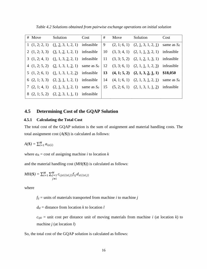
Table 4.2 Solutions obtained from pairwise exchange operations on initial solution .................. 16

Table 4.3 Tabu list after iteration 1 ............................................................................................... 23

Table 4.4 Drop/add neighborhood in iteration 2 ........................................................................... 23

Table 4.5 Pairwise exchange neighborhood in iteration 2 ............................................................ 23

Table 4.6 Tabu list after iteration 2 ............................................................................................... 24

Table 5.1 Setting Initial Temperature for SA Heuristics ............................................................. 28

Table 5.2 Results with N(t) = 10% of the size of the neighborhood ............................................ 29




Table 5.6 Results with N(t) = 50% of the size of the neighborhood ........................................... 28

Table 5.7 Bar Chart with Percent Deviation for Different values of N(t) .................................... 34

Table 5.8 Results from SA Heuristics with Drop/Add Neighborhood ......................................... 36

Table 5.9 Bar Chart with Percent Deviations ............................................................................... 37

Table 5.10 Results from SA Heuristics with Both Neighborhoods .............................................. 38

Table 5.11a Results from TS Heuristics with Drop/Add Neighborhood (tabusize =0.02NBHD) 39

Table 5.11b Results from TS Heuristics with Drop/Add Neighborhood (tabusize =0.03NBHD) 40

Table 5.12 Results Obtained from TS Heuristics with Drop/Add where tabusize = 0.02NBHD or

0.03NBHD .................................................................................................................................... 41

Table 5.13 Results from TS Heuristics with Both Neighborhoods .............................................. 42

Table 5.14 Summary of the Results .............................................................................................. 43

Table 5.15 Comparison of Results for the Proposed Heuristics ................................................... 44

Table 5.16 Comparison of Percent Deviations for the Proposed Heuristics................................. 44

vi

LIST OF FIGURES

Figure 1.1 Different types of facility layouts .................................................................................. 1

Figure 1.2 Simple classification of facility layout problems .......................................................... 2

Figure 1.3 Example of a layout configuration ................................................................................ 4

Figure 3.1 Solution of the GQAP ................................................................................................. 11

1

CHAPTER 1

INTRODUCTION

1.1 The Facility Layout Problem

The facility layout problem (FLP) is defined as the placement of facilities in a plant area, with the

aim of determining the most effective arrangement in accordance with some criteria or objectives

under certain constraints, such as shape, size, orientation, and pick-up/drop-off point of the

facilities.

The facility layout problems can be of different types. Different types of layouts are shown in

Figure 1.1. Figure 1.1(a) shows a quadratic assignment problem (QAP) where all the departments

are equal and only one machine is assigned to each location. Figure 1.1(b) shows an unequal area

facility layout problem (UFLP) where we have rectangular grids and each machine is assigned a

number of grids based on their area requirement.

M15 M5 M11 M2

M6 M1 M4 M13 M4 M2 M5

M14 M8 M12 M7

M10 M3 M16 M9 M1 M3

(a) QAP (Discrete) (b) UAFLP (Discrete)

M1,5,6 M4 D1 D4

M2 M3,7 D2 D5 D3

(c) GQAP (Discrete) (d) Continuous

Figure 1.1: Different types of facility layouts

Figure 1.1(c) shows the generalized quadratic assignment problem (GQAP) where we have

unequal area locations and more than one machine can be assigned to one location. Note, the first

2

one (Figure 1.1(a)) deals with equal area location and the next two (Figures 1.1(b) & (c)) deals

with unequal area locations. All of these are discrete layout problems. However, Figure 1.1(d)

shows a continuous UFLP where several departments with different shapes and areas are located

on a rectangular floor.

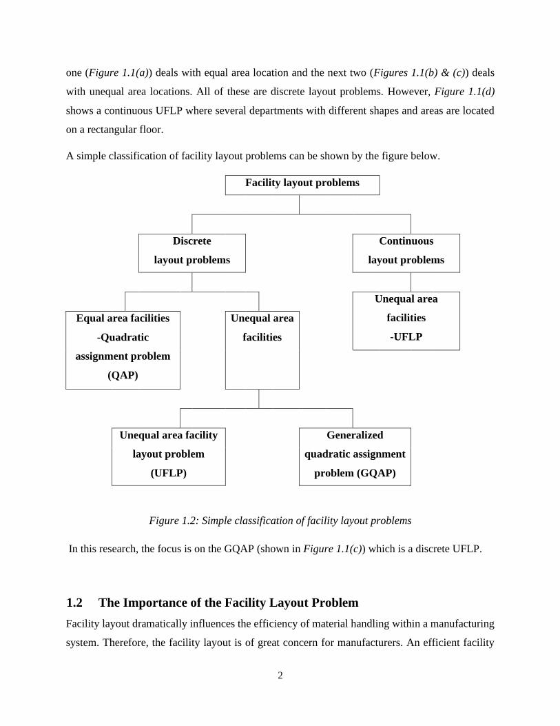
A simple classification of facility layout problems can be shown by the figure below.

Facility layout problems

Discrete

layout problems

Continuous

layout problems

Unequal area

facilities

-UFLP

Equal area facilities

-Quadratic

assignment problem

(QAP)

Unequal area

facilities

Unequal area facility

layout problem

(UFLP)

Generalized

quadratic assignment

problem (GQAP)

Figure 1.2: Simple classification of facility layout problems

In this research, the focus is on the GQAP (shown in Figure 1.1(c)) which is a discrete UFLP.

1.2 The Importance of the Facility Layout Problem

Facility layout dramatically influences the efficiency of material handling within a manufacturing

system. Therefore, the facility layout is of great concern for manufacturers. An efficient facility

3

layout will improve profit and productivity. Moreover, it has been estimated that materials

handling cost is between 20 to 50% of the total operating cost, and effective facility layout planning

can reduce the material handling costs by 10 to 30% (Tompkins et al., 2003).

Since customer demand is constantly changing, the material handling paths and layout of machines

(or departments) are varied constantly. In other words, in order to ensure optimal performance of

a facility, the layout should reflect changes to the system that may occur over time. Therefore, the

FLP exists when either new plants are built or older plants are modified. Francis et al. (1992)

proposed some reasons that may cause the modification of the layout of a facility:

a) Change of the product design.

b) The addition or deletion of a product from the product line.

c) Significant increase or decrease in the demand for a product.

d) Changes on the design of the process.

e) The replacement of equipment.

f) The adoption of new safety standards.

g) Bottlenecks in production.

h) Unexplainable delays and idle time.

i) Excessive temporary storage space.

Therefore, the FLP often occurs and exists for many different reasons. As a result, the facility

layout may need to be modified constantly. The decision of the facility layout is made at the

strategic level and has a long-lasting effect on the manufacturing system. Once the decision is

made, changing the layout of the facility can be very costly. Some of the costs associated with the

re-layout of a facility are cost of rearranging the machines, cost of purchasing or leasing equipment

for rearranging the machines/department, and the cost associated with the loss of production.

Therefore, the importance of the FLP is obvious.

1.3 The Generalized Quadratic Assignment Problem

The generalized quadratic assignment problem (GQAP) is the task of assigning a set of facilities

to a set of locations such that the sum of the assignment and transportation costs is minimized. The

facilities may have different space requirements, and the locations may have varying space

4

capacities. Also, multiple facilities may be assigned to each location such that space capacity is

not exceeded.

The material handling cost depends on the material flows between departments and the distances

between their locations. The most commonly used distance measures for the FLP are rectilinear

and Euclidean. The rectilinear distance between two points (x1, y1) and (x2, y2) is defined as

|𝑥1 − 𝑥2| + |𝑦1 − 𝑦2|, and the Euclidean distance between the two points is defined as

√(𝑥1 − 𝑥2)2 + (𝑦1 − 𝑦2)2. Other distance measures can also be used to determine the distances

between two departments. Nevertheless, in this research the rectilinear distance measure is used to

determine the distance between two departments.

See Figure 1.3 for an example of a layout configuration with 4 locations. Notice the centroid of

each location is given. For example, the centroid of location 4 is (30, 5). Using the rectilinear

distance measure discussed above, the distance between locations 1 and 3 is 17.5 distance units

and between locations 1 and 4 is 27.5 distance units.

20 1

(7.5, 10)

2

(25, 15) 15

10 3

(20, 5)

4

(30, 5) 5

0 5 10 15 20 25 30 35

Figure 1.3: Example of a layout configuration

1.4 Objective of the Thesis

The objectives of this research are given as follows:

1. To develop a tabu search (TS) heuristic for the GQAP.

2. To develop a simulated annealing (SA) heuristic for the GQAP.

3. To test the performance of the heuristics by solving test problems taken from the literature.

4. To compare the performances of the two heuristics.

5

CHAPTER 2

LITERATURE REVIEW

2.1 Introduction

A good number of papers have been published on solving FLPs. But unlike QAP, GQAP literature

is very limited. Exact methods cannot achieve optimal solutions for large scale problems.

Heuristics are used to obtain good quality solutions in short computation times. However, the

optimality of the solutions are not guaranteed by heuristic approaches. The literature review can

be divided in two sections. The first one reviews exact methods and heuristic methods for GQAPs

and their applications. And the second one is a brief review for tabu search (TS) and simulated

annealing (SA) metaheuristics used in different types of FLPs.

2.2 Generalized Quadratic Assignment Problem (GQAP)

2.2.1 Exact Methods

Lee and Ma (2004) presented the first formulation for the GQAP. The authors presented three

methods for the linearization of the formulation and a branch and bound algorithm to optimally

solve the GQAP. Hahn et al. (2008) presented a new algorithm to optimally solve the GQAP.

Pessoa et al. (2010) presented two exact algorithms for the GQAP which combine a previously

proposed branch and bound scheme with a new Lagrangean relaxation procedure over a known

RLT formulation.

2.2.2 Heuristic Methods

Cordeau et al. (2006) presented a linearization of the GQAP formulation as well as a memetic

heuristic for the GQAP, which combines genetic algorithms (Holland,1975) and tabu search

(Glover, 1986). Mateus et al. (2011) proposed several GRASP (greedy randomized adaptive search

procedures) with path-relinking heuristics for the GQAP using different construction, local search,

and path-relinking procedures (GRASP-PR). McKendall and Li (2017) presented an application

of the GQAP for assigning a set of machines to a set of locations on the plant floor. Also, the

authors developed a TS heuristic using different construction algorithms. McKendall (2008)

presented three tabu search heuristics for a dynamic space allocation problem (DSAP) where each

of the proposed heuristics outperformed the heuristics available in the literature for the DSAP. The

DSAP is a layout-type problem that assigns items (project activity resources) to locations (either

6

work or storage spaces) during a multi-period planning horizon such that the cost of rearranging

the items is minimized.

2.2.3 Applications

Apart from facility layouts we have multiple application of the GQAP. Cordeau et al. (2006)

presented an application which uses the GQAP to manage containers in a storage yard (assign M

container groups to N storage areas). Cordeau et al. (2007) considered the service allocation

problem as a GQAP with side constraints. Unal and Uysal (2014) used the GQAP to design a

curriculum at a university. GQAP can also be used to assign maintenance activities and their

required resources to workspaces and their idle resources to storage locations inside the reactor

containment building during planned outages at a nuclear power plant (McKendall and Jaramillo,

2006).

2.3 Metaheuristics for the FLP

2.3.1 Tabu Search

In different types of FLPs, the TS has been widely used in optimizing material handling cost,

utilization of space, minimization of re-layout cost for both single- and multi-objective problems

(Abdinnour-Helm and Hadley, 2000; McKendall and Hakobyan, 2010; Scholz et al., 2009; Seo et

al., 2006; Yang et al., 1999). TS is also deployed for optimizing single row fixed layout design

problem (a special class of FLP) by Samarghandi and Eshghi (2010). Liang and Chao (2008)

proposed a special different intensification and diversification strategies, which shows better

convergence of searching to get proper arrangement of facilities. Improved TS algorithm with

intensification, reconstruction and solution acceptance operation was proposed by Singh (2009),

which gives comparative result with respect to some benchmark problems found in QAP-based

FLP literature.

2.3.2 Simulated Annealing

SA is being used by the researchers in the field, starting from manufacturing cell design to multi-

objective optimization of dynamic and static behaviour of FLP irrespective of whether there are

equal or unequal sized facilities (Castillo and Peters, 2003; Dong et al., 2009; Ioannou, 2007; Sahin

and Türkbey, 2009; Sahin et al., 2010; Souilah, 1995). Hybrid method of SA with TS (Sugiyono,

2006), SA and GA (Matsuzaki et al., 1999) helps to avoid high computational cost (Mir and Imam,

7

2001) and improves the solution. McKendall et al., (2006) developed two SA algorithms for

dynamic facility layout problems. A basic SA heuristic for the DFLP, and an SA heuristic with a

look-ahead/look-back strategy. Gunawan et al. (2014) solved QAP using GRASP and improved

the solution using a hybrid SA-TS algorithm. Privault et al. (1998) and Hamam et al. (2000) solved

GAP using simulated annealing metahuristics.

2.4 Proposed Tabu Search (TS) Heuristic

As mentioned above in the GQAP literature review, a TS heuristic has been presented for the

GQAP. In the TS heuristic presented in McKendall and Li (2017), the best admissible move is

selected randomly among the top solutions at each iteration, to add randomness to diversify the

search. This is a type of probabilistic TS heuristic and is not considered in this thesis. In other

words, in the proposed TS heuristic the best admissible move is selected at each iteration. Also,

McKendall and Li (2017) added even more diversification to their TS heuristic by generating a set

of diverse initial solutions. In the proposed TS heuristic, only one initial solution is generated. For

these reasons the proposed TS heuristic is more restricted. That is, the proposed TS heuristic

presented in this thesis is deterministic.

2.5 Contributions of the Thesis to the GQAP Literature

The GQAP literature is very limited and there in no SA algorithm developed for the GQAP.

Therefore, the contributions of this thesis, to the GQAP literature, is given as follows.

1. Development of a SA heuristic for the GQAP.

2. Improvement of the best found solutions for 3 test problems taken from the literature.

8

CHAPTER 3

PROBLEM DEFINITION

3.1 Problem Definition

There are M machines to be installed in N locations (M ≥ N) in a department. The machines have

different space requirements and the locations have varying space capacities. Multiple machines

can be assigned to each location such that space capacity is not exceeded. The problem is to assign

the machines to the locations such that the total cost (i.e., the sum of installation cost and material

handling costs) is minimized.

3.2 Problem Assumptions

The assumptions for the GQAP are as follows:

1. The layout configuration is given.

2. Machines and locations may be of unequal sizes.

3. The locations have rectangular areas.

4. Material flows between machines are given.

5. The distances between locations are known.

6. The area requirements for the machines are known.

7. The layout representation is discrete.

8. The objective is to minimize the sum of the installation and material handling costs.

3.3 Mathematical Formulation

The formulation of the GQAP from McKendall and Li (2017) is given below and is an adaptation

of the model presented by Lee and Ma (2004).

Minimize z = ∑ ∑ 𝑎𝑖𝑘𝑥𝑖𝑘𝑁𝑘=1

𝑀𝑖=1 + ∑ ∑ ∑ ∑ 𝑐𝑖𝑗𝑘𝑙𝑓𝑖𝑗𝑑𝑘𝑙

𝑁𝑙=1𝑙≠𝑘

𝑁𝑘=1

𝑀𝑗=1𝑗≠𝑖

𝑀𝑖=1 𝑥𝑖𝑘𝑥𝑗𝑙 (1)

Subject to ∑ 𝑥𝑖𝑘 = 1𝑁𝑘=1 , for i=1,…,M (2)

∑ 𝑟𝑖𝑥𝑖𝑘 <= 𝐶𝑘𝑀𝑖=1 , for k=1,…,N (3)

xik= 0 or 1, for i=1,…,M and k=1,…,N (4)

9

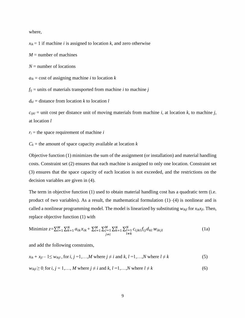
where,

xik = 1 if machine i is assigned to location k, and zero otherwise

M = number of machines

N = number of locations

aik = cost of assigning machine i to location k

fij = units of materials transported from machine i to machine j

dkl = distance from location k to location l

cijkl = unit cost per distance unit of moving materials from machine i, at location k, to machine j,

at location l

ri = the space requirement of machine i

Ck = the amount of space capacity available at location k

Objective function (1) minimizes the sum of the assignment (or installation) and material handling

costs. Constraint set (2) ensures that each machine is assigned to only one location. Constraint set

(3) ensures that the space capacity of each location is not exceeded, and the restrictions on the

decision variables are given in (4).

The term in objective function (1) used to obtain material handling cost has a quadratic term (i.e.

product of two variables). As a result, the mathematical formulation (1)–(4) is nonlinear and is

called a nonlinear programming model. The model is linearized by substituting wikjl for xikxjl. Then,

replace objective function (1) with

Minimize z=∑ ∑ 𝑎𝑖𝑘𝑥𝑖𝑘𝑁𝑘=1

𝑀𝑖=1 + ∑ ∑ ∑ ∑ 𝑐𝑖𝑗𝑘𝑙𝑓𝑖𝑗𝑑𝑘𝑙

𝑁𝑙=1𝑙≠𝑘

𝑁𝑘=1

𝑀𝑗=1𝑗≠𝑖

𝑀𝑖=1 𝑤𝑖𝑘𝑗𝑙 (1a)

and add the following constraints,

xik + xjl – 1≤ wikjl , for i, j =1,…,M where j ≠ i and k, l =1,…,N where l ≠ k (5)

wikjl ≥ 0, for i, j = 1,…, M where j ≠ i and k, l =1,…,N where l ≠ k (6)

10

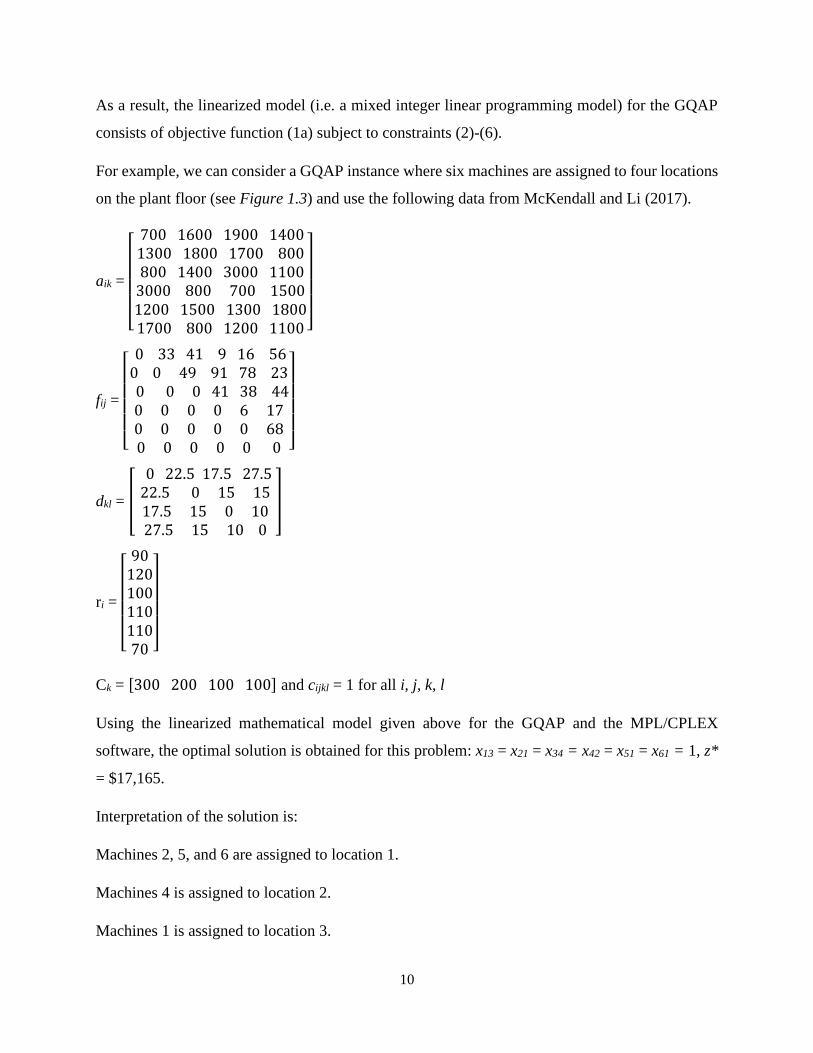
As a result, the linearized model (i.e. a mixed integer linear programming model) for the GQAP

consists of objective function (1a) subject to constraints (2)-(6).

For example, we can consider a GQAP instance where six machines are assigned to four locations

on the plant floor (see Figure 1.3) and use the following data from McKendall and Li (2017).

aik =

[ 700 1600 1900 14001300 1800 1700 800 800 1400 3000 11003000 800 700 15001200 1500 1300 18001700 800 1200 1100 ]

fij =

[ 0 33 41 9 16 560 0 49 91 78 23 0 0 0 41 38 440 0 0 0 6 170 0 0 0 0 680 0 0 0 0 0 ]

dkl = [

0 22.5 17.5 27.5 22.5 0 15 1517.5 15 0 1027.5 15 10 0

]

ri =

[ 9012010011011070 ]

Ck = [300 200 100 100] and cijkl = 1 for all i, j, k, l

Using the linearized mathematical model given above for the GQAP and the MPL/CPLEX

software, the optimal solution is obtained for this problem: x13 = x21 = x34 = x42 = x51 = x61 = 1, z*

= $17,165.

Interpretation of the solution is:

Machines 2, 5, and 6 are assigned to location 1.

Machines 4 is assigned to location 2.

Machines 1 is assigned to location 3.

11

Machine 3 is assigned to location 4.

The solution of the GQAP instance is shown in Figure 3.1.

20 1

M2,5,6

2

M4 15

10 3

M1

4

M3 5

0 5 10 15 20 25 30 35

Figure 3.1: Solution of the GQAP Instance

The sum of total installation cost and total material handling cost is z* = $17,165 where

total installation cost = ∑ ∑ 𝑎𝑖𝑘𝑥𝑖𝑘4𝑘=1

6𝑖=1 = $8,000

and total material handling cost = ∑ ∑ ∑ ∑ 𝑐𝑖𝑗𝑘𝑙𝑓𝑖𝑗𝑑𝑘𝑙4𝑙=1𝑙≠𝑘

4𝑘=1

6𝑗=1𝑗≠𝑖

6𝑖=1 𝑤𝑖𝑘𝑗𝑙 = $9,165.

3.4 Combinatorial Optimization Problem (COP) Model

COPs are problems in which all or some of the decision variables are discrete. For the GQAP the

COP model is given below:

Minimize TC(S) = ∑ 𝑎𝑖𝑠(𝑖) + ∑ ∑ 𝑐𝑖𝑗𝑠(𝑖)𝑠(𝑗)𝑓𝑖𝑗𝑑𝑠(𝑖)𝑠(𝑗)𝑀𝑗=1𝑗≠𝑖

𝑀𝑖=1

𝑀𝑖=1 (7)

Subject to ∑ 𝑟𝑖 ≤ 𝐶𝑘∀𝒊 𝒔.𝒕. 𝒔(𝒊)=𝒌 for k = 1, 2, …, N (8)

where,

J = set of machines |J| = M = number of machines

K = set of locations |K| = N = number of locations

The solution representation is: S = {S(1), S(2), … , S(M)} where S(i) = k, i.e. machine i is assigned

to location k.

12

Objective function (7) minimizes the total cost of the solution S. Constraint set (8) ensures that the

capacity of each location is not violated.

The solution obtained in Section 3.3 for the GQAP instance can be represented as S = (3, 1, 4, 2,

1, 1) which indicates machines 2, 5, and 6 are assigned to location 1, machines 4 is assigned to

location 2, machines 1 is assigned to location 3, and machine 3 is assigned to location 4. Also,

total cost of solution is TC(S) = $17,165.

13

CHAPTER 4

METHODOLOGY

4.1 Introduction

Metaheuristics can improve the performance of many other heuristics. Tabu search (Glover, 1986)

is an aggressive metaheuristic that guides a local search out of local optimal while simulated

annealing (Metropolis et al., 1953) uses a probabilistic approach to obtain the same end. In this

thesis, a tabu search (TS) and a simulated annealing (SA) heuristic are developed to solve the COP

model presented in the previous section to solve the GQAP.

4.2 Solution Representation for the GQAP

Recall, the solution representation for the GQAP is defined as follows:

S = {S(1), S(2), … , S(M)}

where

S = solution of the GQAP

M = number of machines

S(i) = k, i.e. machine i is assigned to location k.

Next, a construction algorithm is presented for the GQAP.

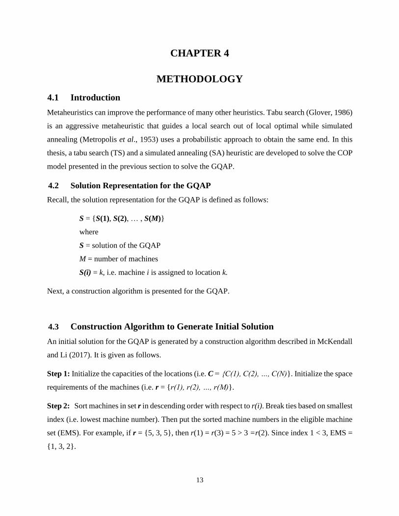
4.3 Construction Algorithm to Generate Initial Solution

An initial solution for the GQAP is generated by a construction algorithm described in McKendall

and Li (2017). It is given as follows.

Step 1: Initialize the capacities of the locations (i.e. C = {C(1), C(2), …, C(N)}. Initialize the space

requirements of the machines (i.e. r = {r(1), r(2), …, r(M)}.

Step 2: Sort machines in set r in descending order with respect to r(i). Break ties based on smallest

index (i.e. lowest machine number). Then put the sorted machine numbers in the eligible machine

set (EMS). For example, if r = {5, 3, 5}, then r(1) = r(3) = 5 > 3 =r(2). Since index 1 < 3, EMS =

{1, 3, 2}.

14

Step 3a: Set k = 1 where k = location number.

Step 3b: If k > N (N = number of locations), then go to step 5b. Else, go to position 1 of EMS

(i.e. set p = 1).

Step 4: Set i = the machine in position p of set EMS.

Step 5a: If r(i) ≤ C(k), then

1. Assign machine i to location k (i.e. set s(i) = k), and set C(k) = C(k) – r(i);

2. Remove machine i from EMS. If EMS is empty, then go to step 5b;

3. If C(k) < r(i) for Last (i) in set EMS, then set k = k + 1, and go to step 3b; Else, go to

step 4. Else, set p = p + 1, and go to step 4.

Step 5b: Terminate algorithm. If EMS is empty, then display feasible solution S. Else, display

“No feasible solution!”

For the GQAP instance mentioned before, the solution generated using this construction algorithm

is S0 = (2, 1, 3, 1, 2, 1) where total cost of this solution is TC(S0) = $21,255. Recall, the optimal

solution obtained using MPL/CPLEX and the mathematical formulation (objective function (1a)

subject to constraints (2)-(6)) presented in Chapter 3 is S = (3, 1, 4, 2, 1, 1) where TC(S) = $17,165.

4.4 Neighborhood Structures

A neighborhood of a solution S0 is a set of solutions that can be obtained from S0 by a simple

operation or move. In our proposed metaheuristics we used two types of neighborhood structures

as defined in McKendall and Li (2017): drop/add and pairwise exchange.

4.4.1 Drop/Add Neighborhood Structure

Drop/add neighborhood considers a simply removal of an element and addition of an element to

the set of solution variables. Using the notation taken from McKendall and Li (2017), the drop/add

operation (u, v: v’) represents exchanging (dropping) location v assigned to machine u with

(adding) location v’. For example, if S0 = {2, 1, 3, 1, 2, 1}, as obtained from using the construction

algorithm presented above to solve the 6 machines 4 locations GQAP instance, then the drop/add

operation (1, 2; 3) produces the solution {3, 1, 3, 1, 2, 1}. In other words, machine 1 assigned to

location 2 is reassigned to location 3. Since there are M = 6 machines and N = 4 locations, and

15

each machine is already assigned to one location, there are N-1 = 3 possible drop/add operations

for each machine. Therefore, there will be M(N-1) = 6(3) = 18 possible drop/add operations. See

Table 4.1 (similar to Table 6 in McKendall and Li, 2017) for all possible drop/add operations on

solution S0 = (2, 1, 3, 1, 2, 1).

Table 4.1 Solutions obtained from drop/add operations on initial solution

# Move Solution Cost # Move Solution Cost

1 (1, 2; 1) (1, 1, 3, 1, 2, 1) infeasible 10 (4, 1; 2) (2, 1, 3, 2, 2, 1) infeasible


3 (1, 2; 4) (4, 1, 3, 1, 2, 1) $21,580 12 (4, 1; 4) (2, 1, 3, 4, 2, 1) infeasible






9 (3, 3; 4) (2, 1,4, 1, 2, 1) $20,695 18 (6, 1; 4) (2, 1, 3, 1, 2, 4) $20,495

4.4.2 Pairwise Exchange Neighborhood Structure

Pairwise exchange considers interchanging or swapping two elements in the current solution.

Using the notation taken from McKendall and Li (2017), the pairwise exchange operation (u, v;

u’, v’) represents exchanging location v assigned to machine u with location v’ assigned to machine

u’. If S0 = {2, 1, 3, 1, 2, 1}, then the pairwise exchange operation (1, 2; 4, 1) produces the solution

{1, 1, 3, 2, 2, 1}. In other words, machine 1 assigned to location 2 exchanges locations with

machine 4 assigned to location 1. Since two machines are swapping locations and there are M = 6

machines, there are a combination of M = 6 pick two i.e., M(M−1)/2 = 15 possible pairwise

exchange operations. If v = v’, the solution does not change. Therefore, there are always less than

M(M−1)/2 pairwise exchange operations when a location has more than one machine assigned to

it. See Table 4.2 (similar to Table 7 in McKendall and Li, 2017) for all possible pairwise exchange

operations on solution S0 = (2, 1, 3, 1, 2, 1).

16

Table 4.2 Solutions obtained from pairwise exchange operations on initial solution


1 (1, 2; 2, 1) (1, 2, 3, 1, 2, 1) infeasible 9 (2, 1; 6, 1) (2, 1, 3, 1, 2, 1) same as S0

2 (1, 2; 3, 3) (3, 1, 2, 1, 2, 1) infeasible 10 (3, 3; 4, 1) (2, 1, 1, 3, 2, 1) infeasible


4 (1, 2; 5, 2) (2, 1, 3, 1, 2, 1) same as S0 12 (3, 3; 6, 1) (2, 1, 1, 1, 2, 3) infeasible

5 (1, 2; 6, 1) (1, 1, 3, 1, 2, 2) infeasible 13 (4, 1; 5, 2) (2, 1, 3, 2, 1, 1) $18,050



8 (2, 1; 5, 2) (2, 2, 3, 1, 1, 1) infeasible

4.5 Determining Cost of the GQAP Solution

4.5.1 Calculating the Total Cost

The total cost of the GQAP solution is the sum of assignment and material handling costs. The

total assignment cost (A(S)) is calculated as follows:

A(S) = ∑ 𝑎𝑖𝑠(𝑖)𝑀𝑖=1

where aik = cost of assigning machine i to location k

and the material handling cost (MH(S)) is calculated as follows:

MH(S) = ∑ ∑ 𝑐𝑖𝑗𝑠(𝑖)𝑠(𝑗)𝑓𝑖𝑗𝑑𝑠(𝑖)𝑠(𝑗)𝑀𝑗=1𝑗≠𝑖

𝑀𝑖=1

where

fij = units of materials transported from machine i to machine j

dkl = distance from location k to location l

cijkl = unit cost per distance unit of moving materials from machine i (at location k) to

machine j (at location l)

So, the total cost of the GQAP solution is calculated as follows:

17

TC(S) = A(S)+ MH (S) = ∑ 𝑎𝑖𝑠(𝑖) + ∑ ∑ 𝑐𝑖𝑗𝑠(𝑖)𝑠(𝑗)𝑓𝑖𝑗𝑑𝑠(𝑖)𝑠(𝑗)𝑀𝑗=1𝑗>𝑖

𝑀𝑖=1

𝑀𝑖=1

= ∑ 𝑎𝑖𝑠(𝑖) + ∑ ∑ 𝑐𝑖𝑗𝑠(𝑖)𝑠(𝑗)𝑤𝑖𝑗𝑑𝑠(𝑖)𝑠(𝑗)𝑀𝐽=𝑖+1

𝑀𝑖=1 𝑀

𝑖=1

where wij = fij + fji

4.5.2 Calculating the Change in Total Cost, ΔTC(S)

Once the objective function value (OFV) is obtained for the initial solution, TC(S0), the OFV of

the neighboring solutions, TC(S), can be obtained efficiently by calculating the change in total

cost. The change in total cost is the sum of the change in assignment and material handling costs.

4.5.2.1 ΔTC(S) in Drop/Add Neighborhood

If a solution S is generated in the drop/add neighborhood of S0 by performing the move (u, v: v’),

the change in assignment cost ΔAuv(S) is calculated as follows:

ΔAuv (S) = 𝑎𝑢𝑣 − 𝑎𝑢𝑣′

And the change in material handling cost ΔMHuv(S) is calculated as follows:

ΔMHuv(S) = ∑ 𝑐𝑖𝑢𝑠(𝑖)𝑣𝑤𝑖𝑢𝑀𝑖=1 𝑑𝑆(𝑖)𝑣 − ∑ 𝑐𝑖𝑢𝑠(𝑖)𝑣′𝑤𝑖𝑢

𝑀𝑖=1 𝑑𝑆(𝑖)𝑣′

= ∑ 𝑐𝑖𝑢𝑠(𝑖)𝑣𝑤𝑖𝑢𝑀𝑖=1 [𝑑𝑆(𝑖)𝑣 − 𝑑𝑆(𝑖)𝑣′]

So, the total change in cost after the drop/operation is:

ΔTC = TC (S0) - TC (S) = ΔAuv (S) + ΔMHuv(S)

= (𝑎𝑢𝑣 − 𝑎𝑢𝑣′) + ∑ 𝑐𝑖𝑢𝑠(𝑖)𝑣𝑤𝑖𝑢𝑀𝑖=1 [𝑑𝑆(𝑖)𝑣 − 𝑑𝑆(𝑖)𝑣′]

4.5.2.2 ΔTC(S) in Pairwise Exchange Neighborhood

If a solution S is generated in the pairwise exchange neighborhood of S0 by performing the move

(u, v: u’, v’), the change in assignment cost ΔA’uv(S) is calculated as follows:

ΔA’uv (S) = (𝑎𝑢𝑣 + 𝑎𝑢′𝑣′) − (𝑎𝑢𝑣′ + 𝑎𝑢′𝑣)

And the change in material handling cost ΔMH’uv(S) is calculated as follows:

ΔMH’uv(S) = [∑ 𝑐𝑖𝑢𝑠(𝑖)𝑣𝑤𝑖𝑢𝑀𝑖=1 𝑑𝑆(𝑖)𝑣 + ∑ 𝑐𝑖𝑢′𝑠(𝑖)𝑣′𝑤𝑖𝑢′

𝑀𝑖=1 𝑑𝑆(𝑖)𝑣′] − [∑ 𝑐𝑖𝑢𝑠(𝑖)𝑣′𝑤𝑖𝑢

𝑀𝑖=1 𝑑𝑆(𝑖)𝑣′ +

∑ 𝑐𝑖𝑢′𝑠(𝑖)𝑣𝑤𝑖𝑢′𝑀𝑖=1 𝑑𝑆(𝑖)𝑣]

18

= ∑ 𝑐𝑖𝑢𝑠(𝑖)𝑣[𝑤𝑖𝑢𝑀𝑖=1 (𝑑𝑆(𝑖)𝑣 − 𝑑𝑆(𝑖)𝑣′) + 𝑤𝑖𝑢′ (𝑑𝑆(𝑖)𝑣′ − 𝑑𝑆(𝑖)𝑣)]

So, the total change in cost after the pairwise exchange operation is:

ΔTC = TC(S0) - TC(S) = ΔA’uv(S) + ΔMH’uv(S)

= [(𝑎𝑢𝑣 + 𝑎𝑢′𝑣′) − (𝑎𝑢𝑣′ + 𝑎𝑢′𝑣)] + ∑ 𝑐𝑖𝑢𝑠(𝑖)𝑣[𝑤𝑖𝑢𝑀𝑖=1 (𝑑𝑆(𝑖)𝑣 − 𝑑𝑆(𝑖)𝑣′) + 𝑤𝑖𝑢′ (𝑑𝑆(𝑖)𝑣′ −

𝑑𝑆(𝑖)𝑣)]

4.6 Steepest Descent Local Search Heuristic

The local neighborhood search technique, called the steepest descent local search heuristic, is used

in the proposed metaheuristics to get to the local optima. The steepest descent local search heuristic

for the GQAP is given as follows.

Step 1: Construct a solution, S0 = (S(1), S(2), …, S(M)), using the construction algorithm

presented earlier and obtain its cost, TC(S0).

Step 2: Evaluate all feasible solutions obtained from all possible drop/add operations on S0 and

all possible pairwise exchange operations on S0.

Step 3: Pick best operation/move which gives best feasible neighboring solution, S, with respect

to total cost, TC(S). If TC(S) < TC(S0), set S0 = S, TC(S0) = TC(S), and go to step 2. Else, terminate

heuristic and display local optimum S0.

Next the SA heuristic is presented for the GQAP. Since SA is a probabilistic heuristic, it does not

always converge to a local optimum solution. As a result, the solutions obtained from the proposed

SA heuristic are either improved and/or verified as a local optimum using the steepest descent

local search heuristic presented above.

4.7 Simulated Annealing (SA)

4.7.1 Basic Simulated Annealing

Simulated annealing (SA) algorithms model the process of annealing in solids to optimize complex

functions or systems. In the physical world, annealing is accomplished by heating a solid to an

elevated temperature and then allowing it to cool slowly enough so that the thermal equilibrium is

maintained. Atoms in the material then assume a globally minimum energy state. SA algorithms

have been successfully applied to a variety of problems. The algorithm starts with an initial

19

solution and generates a new solution by changing one or more of the solution variables. The

objective function is then evaluated for the new solution. While a better solution is always accepted

there is a possibility that a worse solution may be accepted based on a probability function

(Metropolis et al., 1953).

The change in energy is expressed as the change in objective function value (OFV), while the

temperature is a control parameter that sets the probability of selection. In the general method, the

temperature is held constant for a prescribed number of iterations to allow the system to gain

“thermal equilibrium” and is then decreased in accordance with a cooling curve. As the

temperature decreases, so does the probability that a worse solution will be accepted. This forces

the algorithm to converge to an optimal, or near optimal, solution.

4.7.2 Outline of SA for the GQAP

SA heuristics starts with an initial solution S0 and its cost TC(S0). Generates a neighboring solution

S randomly. The cost of the neighboring solution TC(S) is obtained and compared to the cost of

the initial solution TC(S0). If the cost of the neighboring solution is better (i.e., TC(S) < TC(S0))

this solution becomes the best solution, and it is used as the starting solution at the next iteration

(i.e., S0 = S). Otherwise, the initial solution S0 is used as the starting solution at the next iteration

with respect to some probability. This process continues until a stopping criterion is reached.

However, strategies, which use a local search technique that allowed accepting non-improving

neighboring solutions, were considered and performed well. This is the idea behind the SA

heuristic and other meta-heuristics. In other words, the idea of annealing is used to accept non-

improving moves (or neighboring solutions S) to avoid getting trapped at a poor local optimum.

In SA, the probability of accepting non-improving moves initially is high, but as the search

proceeds (and the temperature is reduced), the probability of accepting non-improving moves

reduces. An outline of a basic SA heuristic (McKendall et al., 2006) for combinatorial optimization

problems is as follows:

1. Select settings for the heuristic parameters and generate an initial solution S0 and its cost TC(S0).

This solution S0 is defined as the current solution.

2. Obtain a neighboring solution S of the current solution using a move or operation (e..g., drop

add or pairwise exchange move).

20

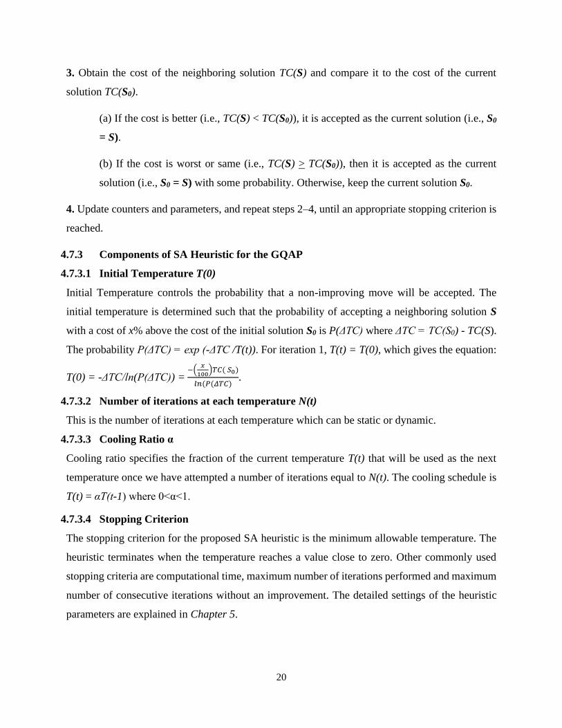
3. Obtain the cost of the neighboring solution TC(S) and compare it to the cost of the current

solution TC(S0).

(a) If the cost is better (i.e., TC(S) < TC(S0)), it is accepted as the current solution (i.e., S0

= S).

(b) If the cost is worst or same (i.e., TC(S) > TC(S0)), then it is accepted as the current

solution (i.e., S0 = S) with some probability. Otherwise, keep the current solution S0.

4. Update counters and parameters, and repeat steps 2–4, until an appropriate stopping criterion is

reached.

4.7.3 Components of SA Heuristic for the GQAP

4.7.3.1 Initial Temperature T(0)

Initial Temperature controls the probability that a non-improving move will be accepted. The

initial temperature is determined such that the probability of accepting a neighboring solution S

with a cost of x% above the cost of the initial solution S0 is P(ΔTC) where ΔTC = TC(S0) - TC(S).

The probability P(ΔTC) = exp (-ΔTC /T(t)). For iteration 1, T(t) = T(0), which gives the equation:

T(0) = -ΔTC/ln(P(ΔTC)) = −(

𝑥

100)𝑇𝐶( 𝑆0)

𝑙𝑛(𝑃(𝛥𝑇𝐶).

4.7.3.2 Number of iterations at each temperature N(t)

This is the number of iterations at each temperature which can be static or dynamic.

4.7.3.3 Cooling Ratio α

Cooling ratio specifies the fraction of the current temperature T(t) that will be used as the next

temperature once we have attempted a number of iterations equal to N(t). The cooling schedule is

T(t) = αT(t-1) where 0<α<1.

4.7.3.4 Stopping Criterion

The stopping criterion for the proposed SA heuristic is the minimum allowable temperature. The

heuristic terminates when the temperature reaches a value close to zero. Other commonly used

stopping criteria are computational time, maximum number of iterations performed and maximum

number of consecutive iterations without an improvement. The detailed settings of the heuristic

parameters are explained in Chapter 5.

21

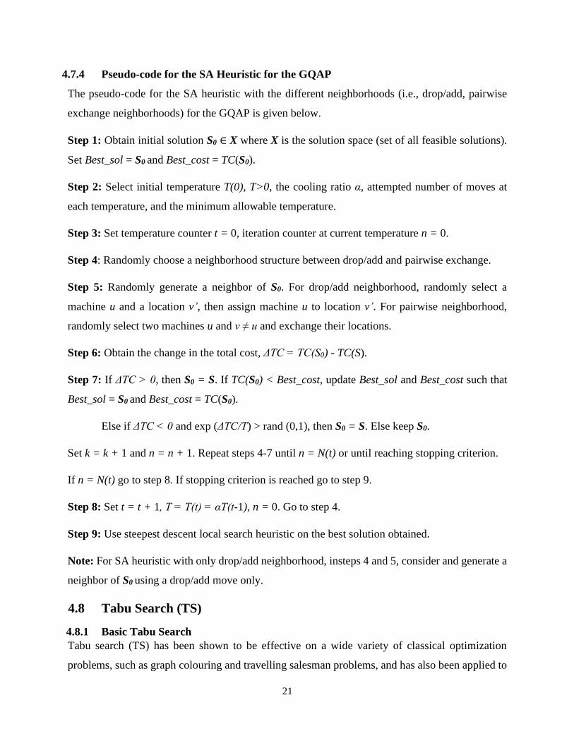
4.7.4 Pseudo-code for the SA Heuristic for the GQAP

The pseudo-code for the SA heuristic with the different neighborhoods (i.e., drop/add, pairwise

exchange neighborhoods) for the GQAP is given below.

Step 1: Obtain initial solution S0 ∈ X where X is the solution space (set of all feasible solutions).

Set Best_sol = S0 and Best_cost = TC(S0).

Step 2: Select initial temperature T(0), T>0, the cooling ratio α, attempted number of moves at

each temperature, and the minimum allowable temperature.

Step 3: Set temperature counter t = 0, iteration counter at current temperature n = 0.

Step 4: Randomly choose a neighborhood structure between drop/add and pairwise exchange.

Step 5: Randomly generate a neighbor of S0. For drop/add neighborhood, randomly select a

machine u and a location v’, then assign machine u to location v’. For pairwise neighborhood,

randomly select two machines u and v ≠ u and exchange their locations.

Step 6: Obtain the change in the total cost, ΔTC = TC(S0) - TC(S).

Step 7: If ΔTC > 0, then S0 = S. If TC(S0) < Best_cost, update Best_sol and Best_cost such that

Best_sol = S0 and Best_cost = TC(S0).

Else if ΔTC < 0 and exp (ΔTC/T) > rand (0,1), then S0 = S. Else keep S0.

Set k = k + 1 and n = n + 1. Repeat steps 4-7 until n = N(t) or until reaching stopping criterion.

If n = N(t) go to step 8. If stopping criterion is reached go to step 9.

Step 8: Set t = t + 1, T = T(t) = αT(t-1), n = 0. Go to step 4.

Step 9: Use steepest descent local search heuristic on the best solution obtained.

Note: For SA heuristic with only drop/add neighborhood, insteps 4 and 5, consider and generate a

neighbor of S0 using a drop/add move only.

4.8 Tabu Search (TS)

4.8.1 Basic Tabu Search

Tabu search (TS) has been shown to be effective on a wide variety of classical optimization

problems, such as graph colouring and travelling salesman problems, and has also been applied to

22

practical problems such as scheduling and electronic circuit design. The method uses aspiration

levels and tabu restrictions which will be discussed below. The search method in the proposed

implementation is a steepest descent algorithm. It explores the set of feasible solutions by moving

from a solution to its best neighbor (the solution with the best objective function value in a

neighborhood), even if this results in a worst objective function value. The short-term memory

contains representations of certain numbers of recent moves (formed as a tabu list). These moves

are forbidden or declared as tabu restricted for a number of iterations which is known as the tabu

duration. As the search progresses the list is updated on a first in-last out basis so that the list

remains a fixed size. It is the short-term memory and the notion of tabu restriction that provide the

capability to escape local optima. The algorithm is run for a prescribed number of iterations or a

prescribed duration of time and then the best solution generated so far is chosen. In this research,

a TS heuristic is presented similar to the TS used in McKendall and Li (2017). The different

between two will be discussed below.

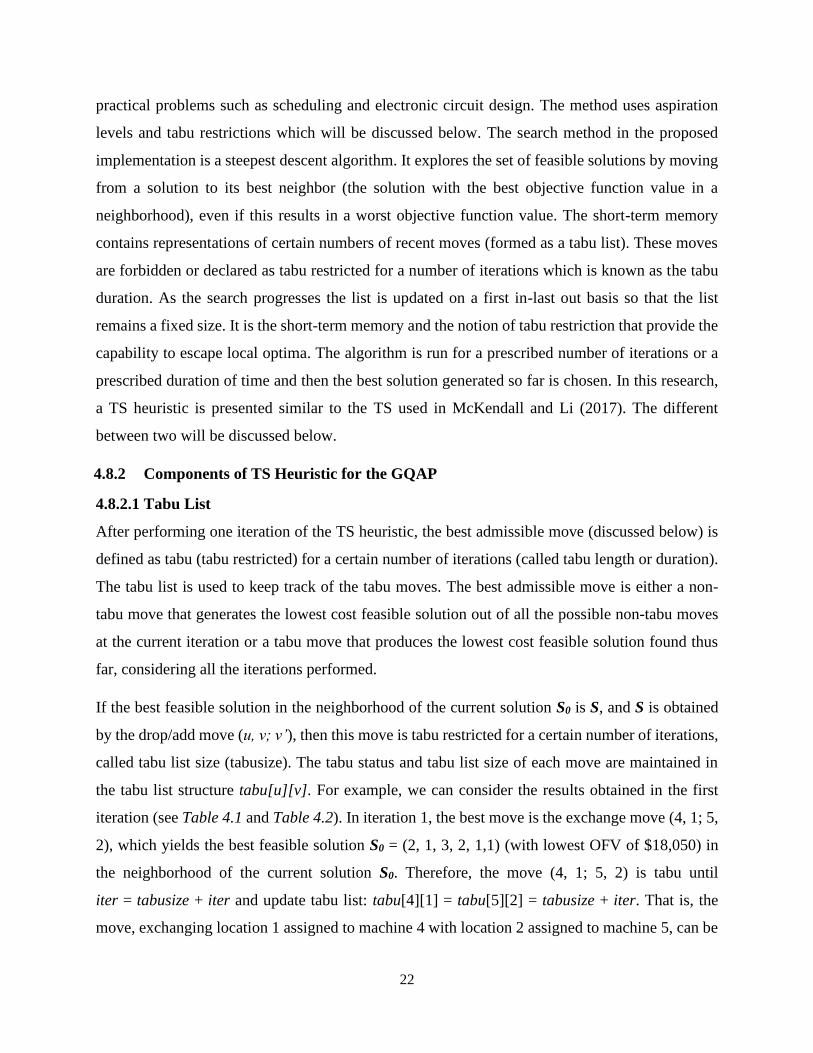
4.8.2 Components of TS Heuristic for the GQAP

4.8.2.1 Tabu List

After performing one iteration of the TS heuristic, the best admissible move (discussed below) is

defined as tabu (tabu restricted) for a certain number of iterations (called tabu length or duration).

The tabu list is used to keep track of the tabu moves. The best admissible move is either a non-

tabu move that generates the lowest cost feasible solution out of all the possible non-tabu moves

at the current iteration or a tabu move that produces the lowest cost feasible solution found thus

far, considering all the iterations performed.

If the best feasible solution in the neighborhood of the current solution S0 is S, and S is obtained

by the drop/add move (u, v; v’), then this move is tabu restricted for a certain number of iterations,

called tabu list size (tabusize). The tabu status and tabu list size of each move are maintained in

the tabu list structure tabu[u][v]. For example, we can consider the results obtained in the first

iteration (see Table 4.1 and Table 4.2). In iteration 1, the best move is the exchange move (4, 1; 5,

2), which yields the best feasible solution S0 = (2, 1, 3, 2, 1,1) (with lowest OFV of $18,050) in

the neighborhood of the current solution S0. Therefore, the move (4, 1; 5, 2) is tabu until

iter = tabusize + iter and update tabu list: tabu[4][1] = tabu[5][2] = tabusize + iter. That is, the

move, exchanging location 1 assigned to machine 4 with location 2 assigned to machine 5, can be

23

performed again when iter > tabusize + iter i.e. iter > tabusize + 1 since current iteration is

iteration 1 (iter = 1). If we consider a tabu size of 6, after iteration 1, the tabu list will look like

Table 4.3.

Table 4.3 Tabu list after iteration 1

1 2 3 4 5 6

1 6+1=7

2 6+1=7

3

4

Table 4.4 Drop/add neighborhood in iteration 2




3 (1, 2; 4) (4, 1, 3, 2, 1, 1) $18,305 12 (4, 2; 4) (2, 1, 3, 4, 1, 1) infeasible






9 (3, 3; 4) (2, 1, 4, 2, 1, 1) $17,460 18 (6, 1; 4) (2, 1, 3, 2, 1, 4) $19,075

Table 4.5 Pairwise exchange neighborhood in iteration 2






5 (1, 2; 6, 1) (1, 1, 3, 2, 1, 2) infeasible 13 (4, 2; 5, 1) (2, 1, 3, 1, 2, 1) $21,255



8 (2, 1; 5, 1) (2, 1, 3, 2, 1, 1) same as S0

24

Similarly, in iteration 2 (see Tables 4.4 and 4.5 for all possible drop/add and pairwise exchange

moves for current solution S0 = (2, 1, 3, 2, 1, 1)), since the best admissible move is the drop/add

move (3, 3; 4), tabu[3][3] = tabusize + iter = tabusize + 2. So the tabu list will be updated

accordingly (see Table 4.6).

Table 4.6 Tabu list after iteration 2

1 2 3 4 5 6

1 6+1=7

2 6+1=7

3 6+2=8

4

4.8.2.2 Aspiration Criterion

The aspiration criterion is a short-term memory strategy used in the tabu search heuristic to

override the tabu restriction. If a move is tabu in the tabu list and produces a solution with a better

objective function value compared to that of the best found solution so far, the move is admissible.

In other words, the tabu restriction is overridden even though the move is tabu.

4.8.2.3 Stopping Criterion

The stopping criterion for the proposed TS heuristic is computational time. This stopping criterion

is used to compare the performances of the proposed TS heuristics with the proposed SA heuristics.

Other commonly used stopping criteria are maximum number of iterations performed and

maximum number of consecutive iterations without an improvement. The detailed settings of the

heuristic parameters are explained in Chapter 5.

4.8.3 Pseudo-code for the TS Heuristic for the GQAP

The TS heuristic proposed here is similar to the TS heuristic proposed in McKendall and Li (2017).

The proposed TS heuristics consider the drop/add neighborhood structure by itself, and both the

drop/add and pairwise exchange neighborhood structures together. However, in McKendall and

Li (2017) the authors consider the drop/add and pairwise exchange neighborhood structures

together. The pseudo-code for the TS heuristic with the different neighborhoods (i.e., drop/add,

pairwise exchange neighborhoods) for the GQAP is given below.

25

The pseudo-code for the TS heuristic with both drop/add and pairwise exchange neighborhood for

the GQAP is given below.

Step 1: Initialize parameters and counters: Set tabu[u][v] = 0, for all u = 1, …, M and v = 1, …,

N. Set tabusize, where tabusize = tabu tenure length. Set MaxTime, where MaxTime = maximum

computational time for the problem before terminating heuristic. Set iter = 0, where iter = iteration

number.

Step 2: Obtain an initial solution S0 = (S(1), S(2), …, S(M)) using the construction algorithm

presented in Section 4.3. Obtain TC(S0) using objective function.

Step 3: Set S* = S0, where S* is the best solution found thus far, and set TC(S*) = TC(S0);

Step 4: Set iter = iter + 1; Find the best admissible move, which gives best feasible solution (S)

in neighborhood S0. Find best feasible solution (S) by considering all possible drop/add and

pairwise exchange operations on S0.

Step 5: Set S0 = S and TC(S0) = TC(S); If TC(S0) < TC(S*), set S* = S0 and TC(S*) = TC(S0).

Step 6: Update tabu list as either tabu[u] [v] = iter + tabusize, if drop/add operation (u, v; v’)

gives best admissible move or tabu[u][v] = tabu[u’][v’] = iter + tabusize, if pairwise exchange

operation (u, v; u’, v’) gives best admissible move.

Step 7: Stopping criterion: If iter < MaxTime, go to Step 4. Else, terminate the heuristic and

return solution S* and total cost of solution TC(S*).

Note: For the TS heuristic with only drop/add neighborhood, consider all possible drop/add moves

only in step 4.

4.9 Comparison of Proposed Meta-heuristics

In TS heuristic the tabu list provides a short-term memory and it is a very deterministic heuristic.

That is, the best admissible move is selected at each iteration. To diversify the search, the best

admissible move in, say, the top 10-25% can be selected at each iteration to add randomness to the

heuristic. This is called the probabilistic TS heuristic. Although this heuristic exists in the

literature, it is not considered in this thesis. On the other hand, SA is very stochastic in nature (i.e.,

26

at each iteration, a move is randomly selected). As a result, an extremely deterministic heuristic

(i.e., TS) and a very stochastic heuristic (i.e., SA) is developed for the proposed GQAP.

After solving problems of different types and sizes, the results obtained from the two diverse

heuristics are compared. To compare the performance of the heuristics, the objective function

value (total cost) as well as time taken to solve the problems should be considered. The

comparisons are discussed in Section 5.4.

27

CHAPTER 5

COMPUTATIONAL RESULTS

5.1 Introduction

The proposed simulated annealing (SA) and tabu search (TS) heuristics were tested on a set of 21

test problems given by Cordeau et. al. (2006). This problem set was also used in other literature

for the GQAP (Mateus et. al., 2011 and McKendall and Li, 2017). The set of test problems contains

problem instances with 20, 30, 35, 40, and 50 machines with locations ranging between 6 and 20

such that the percentages of location area required (i.e. tightness of the capacity constraint) ranges

between 35 and 95. As mentioned previously, the proposed SA and TS heuristics used one of the

construction algorithms presented by McKendall and Li (2017) to generate the initial solutions

(see Section 4.3).

5.2 Computational Environment

The proposed SA and TS heuristics were programmed using MATLAB and executed on a 3.30

GHz Intel Core i5 CPU with 16 GB of RAM under the Microsoft Windows Operating System.

5.3 Setting Parameters

5.3.1 Parameters in Simulated Annealing (SA) Heuristics

Preliminary analyses are performed to determine the SA heuristic parameter settings.

1. Initial Temperature, T(0)

McKendall et. al. (2006) accepted a non-improving neighboring solution (with 25% probability)

with a cost of 10% above the cost of the initial solution to set the initial temperature for a SA

heuristic for a dynamic facility layout problem. Privault et. al. (1998) accepted 80% of the

candidate solutions (i.e., non-improving feasible or infeasible neighboring solutions) for a type of

assignment problem. Note, in this research, only feasible solutions are candidate solutions.

In a preliminary experiment, three problems from the data set with different problem sizes and

different tightness of the capacity constraint are chosen to evaluate the performance of the SA

heuristics with drop/add neighborhood structure. The probability of accepting non-improving

candidate solutions are set at 80% and 90%. The other parameters were fixed for both cases. That

is, the number of iterations at each temperature N(t) is defined to be 10% of the size of the

28

neighborhood, and the cooling parameter α is set to 0.99. See the results of this preliminary study

in Table 5.1 below. The 90% case (i.e., 90% probability of accepting non-improving candidate

solutions) gave better results. Therefore, this is used in the later experiments.

Table 5.1: Setting Initial Temperature for SA Heuristics

Probability

of

accepting

candidate

solutions

Problem

Instances

Best

solution

in

literature

Trial 1 Trial 2 Trial 3 Average

Best

Cost %

Deviation

Cost %

Deviation

80% 20-15-35 1471896 1718733 1781154 1614116 1704668 15.81% 1614116 9.66%

35-15-55 4639128 4913912 5486242 5456673 5285609 13.94% 4913912 5.92%

50-10-95 12845598 18171288 20514591 19860331 19515403 51.92% 18171288 41.46%

90% 20-15-35 1471896 1521604 1506076 1535928 1521203 3.35% 1506076 2.32%

35-15-55 4639128 4819067 4944205 4818008 4860427 4.77% 4818008 3.86%

50-10-95 12845598 18052809 17049092 17380906 17494269 36.19% 17049092 32.72%

2. Minimum Allowable Temperature, Tmin

Minimum allowable temperature is used as the stopping criterion in the proposed SA heuristics.

The minimum allowable temperature, Tmin is set to 0.01, as in McKendall et. al, 2006.

3. Cooling Ratio, α

In the SA heuristics literature, the value of the cooling ratio α is set between 0.9-0.998. In the

experiments below, this value is set to 0.99.

4. Number of iterations at each temperature, N(t)

Using the parameter settings mentioned above, a preliminary experiment was performed to see

how the value of N(t) affects the results. The values of N(t) used are 10%, 20%, 30%, 40% and

50% of the size of the neighborhood. The results are shown in Tables 5.2-5.6. The results equal to

or better than the best found solutions in literature are given in bold font.

29

Table 5.2: Results with N(t) = 10% of the size of the neighborhood

Problem

Instances

Best

solution

in

literature

Trial 1 Trial 2 Trial 3 Trial 4 Trial 5 Trial 6 Best

Results

%

Deviation

20-15-35 1471896 1562334 1666277 1654817 1683947 1633818 1506076 1506076 2.32%

20-15-55 1723638 1774373 1760779 1746373 1765301 1768575 1775879 1746373 1.32%

20-15-75 1967315 2164399 2082325 2197493 2271365 2110196 2097599 2082325 5.85%

30-06-95 5160920 7343965 7396391 7282153 7231103 7261463 7338332 7231103 40.11%

30-07-75 4383923 4866487 4925550 5261271 5162753 5043916 4876711 4866487 11.01%

30-08-55 3501695 3604426 3583662 3640803 3687505 3501695 3859019 3501695 0.00%

30-10-65 3620959 4061961 4015158 3983075 4046989 4317204 4030877 3983075 10.00%

30-20-35 3633644 3470425 3668551 3786653 3712153 3806562 3824489 3470425 -4.49%

30-20-55 3599602 3769255 3811693 3867163 3852868 3626272 3847910 3626272 0.74%

30-20-75 4050938 4186411 4428979 4275888 4050938 4342809 4403353 4050938 0.00%

30-20-95 5726530 7980938 7780961 8055889 7942314 7909580 7780961 7780961 35.88%

35-15-35 4456670 4550406 4560935 4637488 4602290 4756974 4630814 4550406 2.10%

35-15-55 4639128 4935291 4780621 5148577 5005799 4969027 5049512 4780621 3.05%

35-15-75 6301723 6676525 6623197 6543257 6571093 6589578 6606436 6543257 3.83%

35-15-95 6670264 11073897 10502375 10888223 10527428 11600152 11534541 10502375 57.45%

40-07-75 7405793 7853993 7533579 7481964 7675760 7476115 7570414 7476115 0.95%

40-09-95 7667719 9824366 10769720 10357320 10763954 10556437 11343446 9824366 28.13%

40-10-65 7265559 7312813 7265559 7737908 7265559 7390261 7325468 7265559 0.00%

50-10-65 10513029 10716593 10768262 10641717 10624654 10718070 10942884 10624654 1.06%

50-10-75 11217503 12175256 12398118 11902391 12195717 12164193 11939694 11902391 6.11%

50-10-95 12845598 17769538 19658267 15751197 18582569 18149669 17617411 15751197 22.62%

30


Problem

Instances

Best

solution

in

literature


Results

%

Deviation

20-15-35 1471896 1588987 1548769 1562145 1601312 1525718 1521604 1521604 3.38%

20-15-55 1723638 1774373 1764158 1752972 1817353 1782379 1723638 1723638 0.00%

20-15-75 1967315 2041918 2126257 2115180 2057468 2213512 2120431 2041918 3.79%

30-06-95 5160920 7247483 7160004 7412682 7475173 7395715 7497761 7160004 38.74%

30-07-75 4383923 4677043 5347809 5079456 4678065 5166234 4594686 4594686 4.81%

30-08-55 3501695 3532566 3501695 3584958 3532566 3599746 3638030 3501695 0.00%

30-10-65 3620959 3943414 3941497 4006612 3777807 3880017 3976571 3777807 4.33%

30-20-35 3633644 3460504 3731187 3813073 3830739 3742375 3724273 3460504 -4.76%

30-20-55 3599602 3726465 3819853 3622258 3763267 3770997 3746221 3622258 0.63%

30-20-75 4050938 4239695 4233113 4301731 4452933 4210272 4440242 4210272 3.93%

30-20-95 5726530 8034139 7845030 7919961 7606477 8080334 8010218 7606477 32.83%

35-15-35 4456670 4620810 4604970 4538589 4576827 4694835 4544283 4538589 1.84%

35-15-55 4639128 4819067 4876326 4818008 5016659 4954007 4944205 4818008 3.86%

35-15-75 6301723 6585733 6442490 6445856 6392312 6413066 6451959 6392312 1.44%

35-15-95 6670264 10626593 10627451 11146052 10525688 10968883 10937121 10525688 57.80%

40-07-75 7405793 7504465 7664909 7595950 7570121 7559801 7709946 7504465 1.33%

40-09-95 7667719 11306285 9685784 10502930 10540251 10942780 10807231 9685784 26.32%

40-10-65 7265559 7321819 7298103 7385528 7288263 7302026 7360432 7288263 0.31%

50-10-65 10513029 10779442 10637068 10749210 10704071 11054040 10596584 10596584 0.79%

50-10-75 11217503 12012667 12284677 11821395 11752506 12055603 12605241 11752506 4.77%

50-10-95 12845598 17439024 17059700 17530023 18013567 17043366 17355431 17043366 32.68%

31


Problem

Instances

Best

solution

in

literature


Results

%

Deviation

20-15-35 1471896 1559407 1535928 1584946 1519070 1556821 1511402 1511402 2.68%

20-15-55 1723638 1738832 1738832 1761175 1839191 1775879 1751669 1738832 0.88%

20-15-75 1967315 2318448 2391599 2153335 2015529 2058889 2179943 2015529 2.45%

30-06-95 5160920 7409304 7178809 7340597 7191420 7250003 7104924 7104924 37.67%

30-07-75 4383923 5283280 4570820 5047180 4732311 4402834 4718853 4402834 0.43%

30-08-55 3501695 3532566 3501695 3501695 3585428 3622115 3501695 3501695 0.00%

30-10-65 3620959 4126158 4028574 3959570 3693834 3785624 3847868 3693834 2.01%

30-20-35 3633644 3710782 3489490 3724920 3845483 3380252 3791180 3380252 -6.97%

30-20-55 3599602 3679311 3717663 3672132 3664287 3786701 3794916 3664287 1.80%

30-20-75 4050938 4407066 4331100 4263142 4152522 4238119 4336481 4152522 2.51%

30-20-95 5726530 7780929 8300102 8114864 7999346 8071604 7908528 7780929 35.88%

35-15-35 4456670 4568304 4623489 4578428 4475921 4665918 4551509 4475921 0.43%

35-15-55 4639128 4833868 4765403 4817371 4833912 4843301 4843082 4765403 2.72%

35-15-75 6301723 6397501 6496238 6349183 6380077 6390791 6350896 6349183 0.75%

35-15-95 6670264 10611932 11166777 11392651 10630882 10786901 10603120 10603120 58.96%

40-07-75 7405793 7581276 7508405 7608138 7530671 7599048 7592428 7508405 1.39%

40-09-95 7667719 11210421 10736737 10429446 9355239 10624813 11254917 9355239 22.01%

40-10-65 7265559 7321819 7344992 7286973 7405811 7291789 7286973 7286973 0.29%

50-10-65 10513029 10696816 10513029 10637184 10656900 10654528 10715283 10513029 0.00%

50-10-75 11217503 12177476 12018025 12439906 12413982 12042092 11967764 11967764 6.69%

50-10-95 12845598 18274578 18422922 16217825 19025566 18052809 16129920 16129920 25.57%

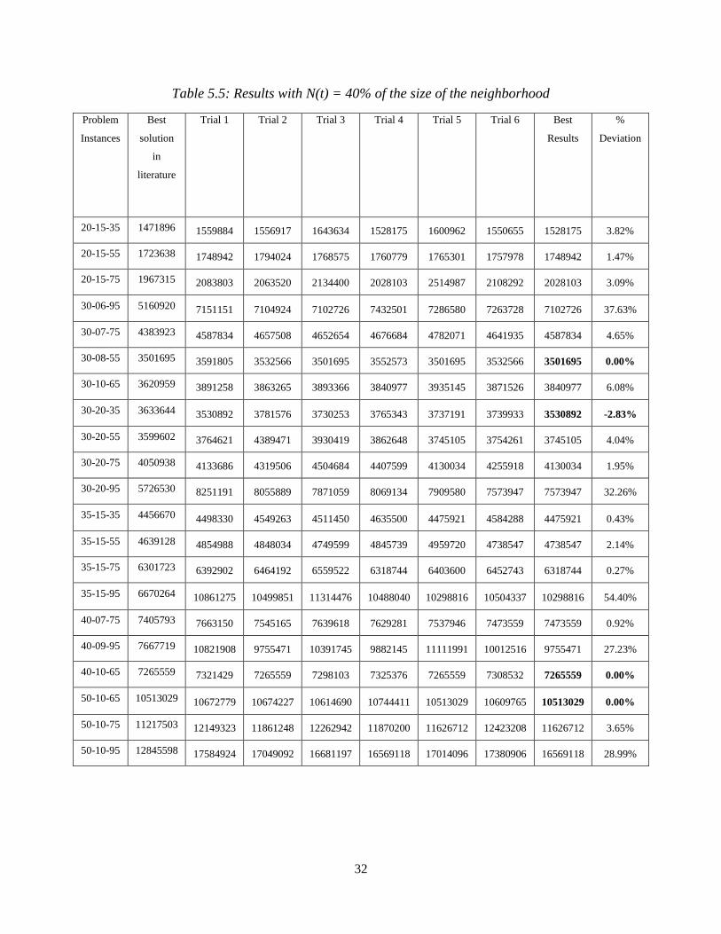
32


Problem

Instances

Best

solution

in

literature


Results

%

Deviation

20-15-35 1471896 1559884 1556917 1643634 1528175 1600962 1550655 1528175 3.82%

20-15-55 1723638 1748942 1794024 1768575 1760779 1765301 1757978 1748942 1.47%

20-15-75 1967315 2083803 2063520 2134400 2028103 2514987 2108292 2028103 3.09%

30-06-95 5160920 7151151 7104924 7102726 7432501 7286580 7263728 7102726 37.63%

30-07-75 4383923 4587834 4657508 4652654 4676684 4782071 4641935 4587834 4.65%

30-08-55 3501695 3591805 3532566 3501695 3552573 3501695 3532566 3501695 0.00%

30-10-65 3620959 3891258 3863265 3893366 3840977 3935145 3871526 3840977 6.08%

30-20-35 3633644 3530892 3781576 3730253 3765343 3737191 3739933 3530892 -2.83%

30-20-55 3599602 3764621 4389471 3930419 3862648 3745105 3754261 3745105 4.04%

30-20-75 4050938 4133686 4319506 4504684 4407599 4130034 4255918 4130034 1.95%

30-20-95 5726530 8251191 8055889 7871059 8069134 7909580 7573947 7573947 32.26%

35-15-35 4456670 4498330 4549263 4511450 4635500 4475921 4584288 4475921 0.43%

35-15-55 4639128 4854988 4848034 4749599 4845739 4959720 4738547 4738547 2.14%

35-15-75 6301723 6392902 6464192 6559522 6318744 6403600 6452743 6318744 0.27%

35-15-95 6670264 10861275 10499851 11314476 10488040 10298816 10504337 10298816 54.40%

40-07-75 7405793 7663150 7545165 7639618 7629281 7537946 7473559 7473559 0.92%

40-09-95 7667719 10821908 9755471 10391745 9882145 11111991 10012516 9755471 27.23%

40-10-65 7265559 7321429 7265559 7298103 7325376 7265559 7308532 7265559 0.00%

50-10-65 10513029 10672779 10674227 10614690 10744411 10513029 10609765 10513029 0.00%

50-10-75 11217503 12149323 11861248 12262942 11870200 11626712 12423208 11626712 3.65%

50-10-95 12845598 17584924 17049092 16681197 16569118 17014096 17380906 16569118 28.99%

33


Problem

Instances

Best

solution

in

literature


Results

%

Deviation

20-15-35 1471896 1558679 1540827 1688644 1577173 1506076 1568709 1506076 2.32%

20-15-55 1723638 1748802 1750956 1749239 1723638 1723638 1723638 1723638 0.00%

20-15-75 1967315 2512615 2136576 2069258 2037924 2046022 2089578 2037924 3.59%

30-06-95 5160920 7115392 7380273 7039637 7473350 6737629 7271187 6737629 30.55%

30-07-75 4383923 4721240 4712002 5193019 4792308 4645271 4918105 4645271 5.96%

30-08-55 3501695 3532566 3717046 3574190 3501695 3501695 3585269 3501695 0.00%

30-10-65 3620959 4132036 3938842 3675880 4061888 3980126 3832514 3675880 1.52%

30-20-35 3633644 3735999 3744394 3697497 3507855 3775495 3379359 3379359 -7.00%

30-20-55 3599602 3681638 3739926 3815328 3794765 3748363 3726853 3681638 2.28%

30-20-75 4050938 4206006 4275035 4344092 4208611 4356155 4445755 4206006 3.83%

30-20-95 5726530 7909580 7780961 8060757 7703063 7854754 7919961 7703063 34.52%

35-15-35 4456670 4518355 4488838 4514053 4494650 4540174 4466588 4466588 0.22%

35-15-55 4639128 4708530 4840727 4657037 4860235 4895690 4863835 4657037 0.39%

35-15-75 6301723 6487853 6458198 6316674 6475040 6301723 6401514 6301723 0.00%

35-15-95 6670264 10995700 10152100 10937121 10657443 11124050 10600533 10152100 52.20%

40-07-75 7405793 7624973 7592188 7481964 7508644 7456976 7520676 7456976 0.69%

40-09-95 7667719 10624137 11771971 11016515 10954067 10891649 10275821 10275821 34.01%

40-10-65 7265559 7308514 7288263 7265559 7305381 7378020 7325376 7265559 0.00%

50-10-65 10513029 10614690 10617874 10614494 10513029 10617874 10616746 10513029 0.00%

50-10-75 11217503 12115902 12302901 12065104 12139666 11832519 12469026 11832519 5.48%

50-10-95 12845598 17997798 16139493 17915442 17107898 17621964 16884109 16139493 25.64%

The percent deviations obtained in the five tables above are shown in a bar chart. See Table 5.7

below. Notice that N(t) = 50% of the size of the neighborhood performed better for most of the

34

problems. For example, consider the problem instance 35-15-75. The percent deviations are

3.83%, 1.44%, 0.75%, 0.27%, and 0.00% where N(t) = 10%, 20%, 30%, 40% and 50% of the size

of the neighborhood, respectively. But the percent deviations for the problems with high space

capacity utilization are still very high. For example, for the problem instance 35-15-95, the percent

deviations are ranged from 52.20% to 58.96%, which are very high values.

Table 5.7: Bar Chart with Percent Deviation for Different values of N(t)

The value of the cooling ratio, α is now increased to 0.9999 and the minimum allowable

temperature, Tmin is lowered to 0.0001 so that we can explore more solutions and chance of getting

better solutions increases. All parameters used for the proposed SA heuristics are summarized

below.

-20.00%

-10.00%

0.00%

10.00%

20.00%

30.00%

40.00%

50.00%

60.00%

70.00%Percent Deviation

10% of NBHD 20% of NBHD 30% of NBHD 40% of NBHD 50% of NBHD

35

Initial temperature, T(0): the probability of accepting a non-improving neighboring solution with

a cost of 10% above the cost of the initial solution is 90%. See section 4.7.3.1 for the formula

and explanation for calculating T(0) where here x = 10.

Cooling ratio, α = 0.9999

Number of iterations at each temperature N(t) = 50% of the size of the neighborhood

Minimum allowable temperature, Tmin = 0.0001

These parameter settings are used to test the performances of the proposed SA heuristics for both

neighborhood structures (i.e., drop/add and pairwise exchange). The results are presented and

discussed below in Section 5.4.1.

5.3.2 Parameters in Tabu Search (TS) Heuristics

1. Tabu size or tabu length

For the proposed TS heuristics with both drop/add and pairwise exchange neighborhood structures,

the tabu length (tabusize) is set to the exact values used in McKendall and Li (2017).

McKendall and Li (2017) obtained the best feasible solutions for the GQAP while using the tabu

length by multiplying the size of the neighborhood by 0.005 to 0.02. Smaller values of tabusize

tend to result in poor solutions, since the TS heuristic either spends too much time repeating the

same moves, or may get trapped at a local optima (i.e. cycling). On the other hand, using a large

value for tabusize results in restricting the solution space too much whereby many potentially good

moves may be overlooked, resulting in poor solutions. The proposed TS heuristics with only

drop/add neighborhood structure used tabusize equal to 0.02 and 0.03 times the size of the

neighborhood.

2. Computational time

The stopping criterion for the proposed TS heuristic is computational time. The maximum

computational time (see Table 5.8 and 5.10) for each problem from SA heuristic is set as the

computational time for the respective problems.

These parameter settings are used to test the performances of the proposed TS heuristics. The

results are presented and discussed below, in Section 5.4.2.

36

5.4 Results

As stated previously, the proposed TS and SA heuristics used the dataset from Cordeau et. al.

(2006) to test the performances of the proposed heuristics. The results are presented below.

5.4.1 Simulated Annealing (SA) Heuristics

The proposed SA heuristics was implemented using the parameter settings mentioned in Section

5.3.1. The results of the SA heuristics with drop/add neighborhood structure is given in Table 5.8.

Table 5.8: Results from SA Heuristics with Drop/Add Neighborhood

Problem

Instances

Trial 1 Trial 2 Trial 3 Trial 4 Trial 5 Average Best Average

Runtime

(seconds)

Maximum

Runtime

(seconds) Cost %

Deviation

Cost %

Deviation

20-15-35 1506076 1539678 1509123 1511402 1511402 1515536.2 2.96% 1506076 2.32% 3831.8 4194.7

20-15-55 1723638 1723638 1723638 1723638 1723638 1723638 0.00% 1723638 0.00% 4092.7 4457.5

20-15-75 1987133 1988689 1988689 1976791 1989271 1986114.6 0.96% 1976791 0.48% 4266.9 4565.4

30-06-95 6416228 6219342 6476590 6513339 6416329 6408365.6 24.17% 6219342 20.51% 1154.6 1212.5

30-07-75 4540060 4640070 4600906 4595501 4400593 4555426 3.91% 4400593 0.38% 2047.1 2287.2

30-08-55 3501695 3501695 3501695 3501695 3501695 3501695 0.00% 3501695 0.00% 2707.6 2962.6

30-10-65 3663198 3746644 3736251 3640684 3713822 3700119.8 2.19% 3640684 0.54% 3557.4 3767.8

30-20-35 3510015 3380252 3451254 3380252 3468225 3437999.6 -5.38% 3380252 -6.97% 8924.0 9672.0

30-20-55 3593105 3626509 3622258 3649512 3660919 3630460.6 0.86% 3593105 -0.18% 9414.6 10907.9

30-20-75 4050938 4116011 4215750 4115879 4107614 4121238.4 1.74% 4050938 0.00% 10405.2 11363.0

30-20-95 7573110 7575493 7573110 7575493 7573110 7574063.2 32.26% 7573110 32.25% 16476.4 17004.0

35-15-35 4456670 4457348 4459912 4464070 4456670 4458934 0.05% 4456670 0.00% 7024.2 7714.4

35-15-55 4713054 4722172 4673657 4639128 4670370 4683676.2 0.96% 4639128 0.00% 7436.5 7974.1

35-15-75 6319838 6319838 6319838 6301723 6332985 6318844.4 0.27% 6301723 0.00% 7846.6 8936.8

35-15-95 9089146 9917835 9089146 10108923 10000498 9641109.6 44.54% 9089146 36.26% 8632.8 10332.0

40-07-75 7466532 7458588 7478567 7469028 7428176 7460178.2 0.73% 7428176 0.30% 2797.8 2956.6

40-09-95 9189719 9619006 9985473 9499848 9546826 9568174.4 24.79% 9189719 19.85% 3658.7 3915.8

40-10-65 7265559 7286973 7274192 7285016 7265559 7275459.8 0.14% 7265559 0.00% 4976.9 5214.0

50-10-65 10513029 10513029 10513029 10513029 10513029 10513029 0.00% 10513029 0.00% 6312.7 6713.1

50-10-75 11967764 11935565 12096401 11482321 11637986 11824007 5.41% 11482321 2.36% 6032.5 6340.1

50-10-95 14278379 15335045 14964326 14115461 14455373 14629717 13.89% 14115461 9.89% 3831.8 6058.7

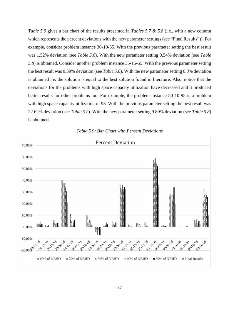
37

Table 5.9 gives a bar chart of the results presented in Tables 5.7 & 5.8 (i.e., with a new column

which represents the percent deviations with the new parameter settings (see “Final Results”)). For

example, consider problem instance 30-10-65. With the previous parameter setting the best result

was 1.52% deviation (see Table 5.6). With the new parameter setting 0.54% deviation (see Table

5.8) is obtained. Consider another problem instance 35-15-55. With the previous parameter setting

the best result was 0.39% deviation (see Table 5.6). With the new parameter setting 0.0% deviation

is obtained i.e. the solution is equal to the best solution found in literature. Also, notice that the

deviations for the problems with high space capacity utilization have decreased and it produced

better results for other problems too. For example, the problem instance 50-10-95 is a problem

with high space capacity utilization of 95. With the previous parameter setting the best result was

22.62% deviation (see Table 5.2). With the new parameter setting 9.89% deviation (see Table 5.8)

is obtained.

Table 5.9: Bar Chart with Percent Deviations

-20.00%

-10.00%

0.00%

10.00%

20.00%

30.00%

40.00%

50.00%

60.00%

70.00%Percent Deviation

10% of NBHD 20% of NBHD 30% of NBHD 40% of NBHD 50% of NBHD Final Results

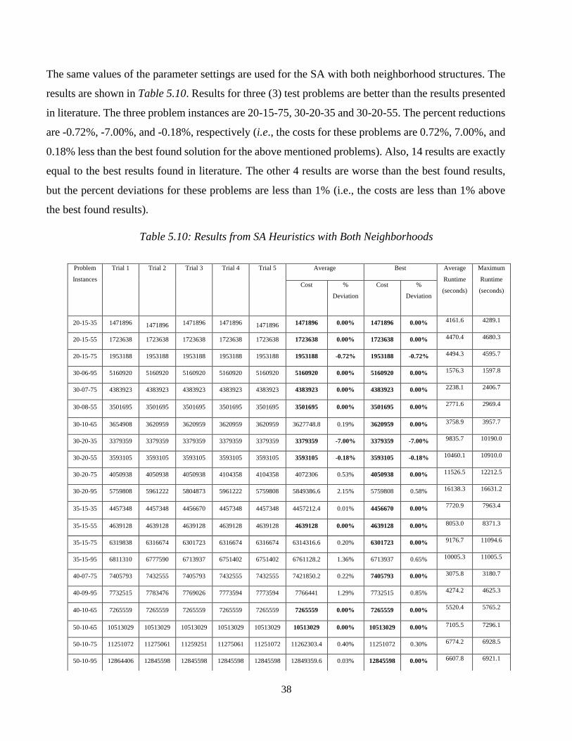
38

The same values of the parameter settings are used for the SA with both neighborhood structures. The

results are shown in Table 5.10. Results for three (3) test problems are better than the results presented

in literature. The three problem instances are 20-15-75, 30-20-35 and 30-20-55. The percent reductions

are -0.72%, -7.00%, and -0.18%, respectively (i.e., the costs for these problems are 0.72%, 7.00%, and

0.18% less than the best found solution for the above mentioned problems). Also, 14 results are exactly

equal to the best results found in literature. The other 4 results are worse than the best found results,

but the percent deviations for these problems are less than 1% (i.e., the costs are less than 1% above

the best found results).

Table 5.10: Results from SA Heuristics with Both Neighborhoods

Problem

Instances

Trial 1 Trial 2 Trial 3 Trial 4 Trial 5 Average Best Average

Runtime

(seconds)

Maximum

Runtime

(seconds) Cost %

Deviation

Cost %

Deviation

20-15-35 1471896 1471896 1471896 1471896 1471896 1471896 0.00% 1471896 0.00% 4161.6 4289.1

20-15-55 1723638 1723638 1723638 1723638 1723638 1723638 0.00% 1723638 0.00% 4470.4 4680.3

20-15-75 1953188 1953188 1953188 1953188 1953188 1953188 -0.72% 1953188 -0.72% 4494.3 4595.7

30-06-95 5160920 5160920 5160920 5160920 5160920 5160920 0.00% 5160920 0.00% 1576.3 1597.8

30-07-75 4383923 4383923 4383923 4383923 4383923 4383923 0.00% 4383923 0.00% 2238.1 2406.7

30-08-55 3501695 3501695 3501695 3501695 3501695 3501695 0.00% 3501695 0.00% 2771.6 2969.4

30-10-65 3654908 3620959 3620959 3620959 3620959 3627748.8 0.19% 3620959 0.00% 3758.9 3957.7

30-20-35 3379359 3379359 3379359 3379359 3379359 3379359 -7.00% 3379359 -7.00% 9835.7 10190.0

30-20-55 3593105 3593105 3593105 3593105 3593105 3593105 -0.18% 3593105 -0.18% 10460.1 10910.0

30-20-75 4050938 4050938 4050938 4104358 4104358 4072306 0.53% 4050938 0.00% 11526.5 12212.5

30-20-95 5759808 5961222 5804873 5961222 5759808 5849386.6 2.15% 5759808 0.58% 16138.3 16631.2

35-15-35 4457348 4457348 4456670 4457348 4457348 4457212.4 0.01% 4456670 0.00% 7720.9 7963.4

35-15-55 4639128 4639128 4639128 4639128 4639128 4639128 0.00% 4639128 0.00% 8053.0 8371.3

35-15-75 6319838 6316674 6301723 6316674 6316674 6314316.6 0.20% 6301723 0.00% 9176.7 11094.6

35-15-95 6811310 6777590 6713937 6751402 6751402 6761128.2 1.36% 6713937 0.65% 10005.3 11005.5

40-07-75 7405793 7432555 7405793 7432555 7432555 7421850.2 0.22% 7405793 0.00% 3075.8 3180.7

40-09-95 7732515 7783476 7769026 7773594 7773594 7766441 1.29% 7732515 0.85% 4274.2 4625.3

40-10-65 7265559 7265559 7265559 7265559 7265559 7265559 0.00% 7265559 0.00% 5520.4 5765.2

50-10-65 10513029 10513029 10513029 10513029 10513029 10513029 0.00% 10513029 0.00% 7105.5 7296.1

50-10-75 11251072 11275061 11259251 11275061 11251072 11262303.4 0.40% 11251072 0.30% 6774.2 6928.5

50-10-95 12864406 12845598 12845598 12845598 12845598 12849359.6 0.03% 12845598 0.00% 6607.8 6921.1

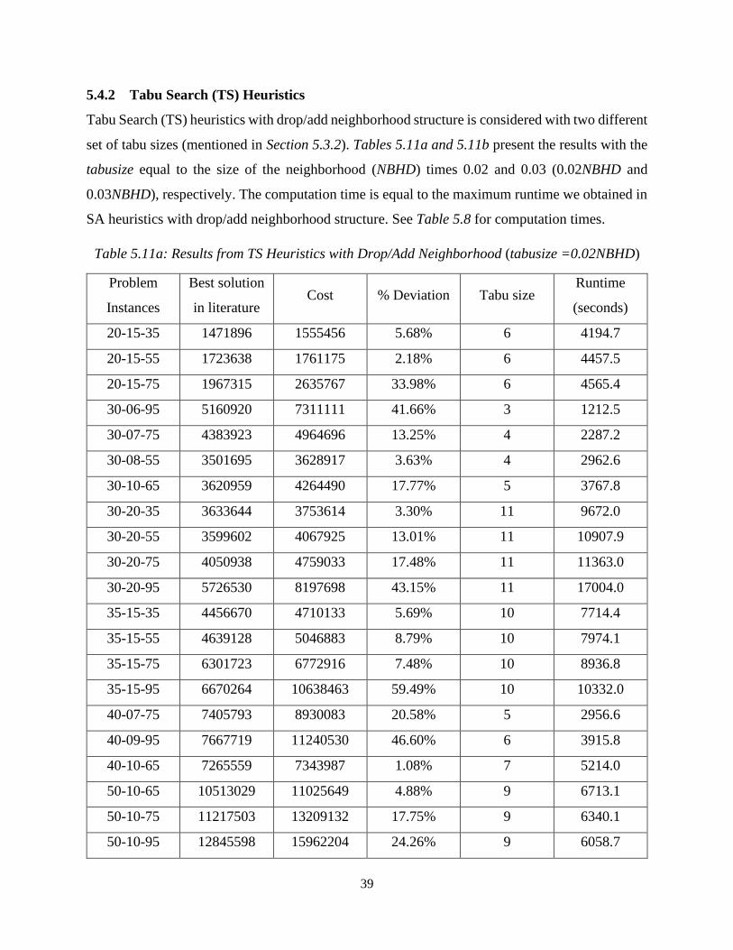
39

5.4.2 Tabu Search (TS) Heuristics

Tabu Search (TS) heuristics with drop/add neighborhood structure is considered with two different

set of tabu sizes (mentioned in Section 5.3.2). Tables 5.11a and 5.11b present the results with the

tabusize equal to the size of the neighborhood (NBHD) times 0.02 and 0.03 (0.02NBHD and

0.03NBHD), respectively. The computation time is equal to the maximum runtime we obtained in

SA heuristics with drop/add neighborhood structure. See Table 5.8 for computation times.

Table 5.11a: Results from TS Heuristics with Drop/Add Neighborhood (tabusize =0.02NBHD)

Problem

Instances

Best solution

in literature Cost % Deviation Tabu size

Runtime

(seconds)

20-15-35 1471896 1555456 5.68% 6 4194.7

20-15-55 1723638 1761175 2.18% 6 4457.5

20-15-75 1967315 2635767 33.98% 6 4565.4

30-06-95 5160920 7311111 41.66% 3 1212.5

30-07-75 4383923 4964696 13.25% 4 2287.2

30-08-55 3501695 3628917 3.63% 4 2962.6

30-10-65 3620959 4264490 17.77% 5 3767.8

30-20-35 3633644 3753614 3.30% 11 9672.0

30-20-55 3599602 4067925 13.01% 11 10907.9

30-20-75 4050938 4759033 17.48% 11 11363.0

30-20-95 5726530 8197698 43.15% 11 17004.0

35-15-35 4456670 4710133 5.69% 10 7714.4

35-15-55 4639128 5046883 8.79% 10 7974.1

35-15-75 6301723 6772916 7.48% 10 8936.8

35-15-95 6670264 10638463 59.49% 10 10332.0

40-07-75 7405793 8930083 20.58% 5 2956.6

40-09-95 7667719 11240530 46.60% 6 3915.8

40-10-65 7265559 7343987 1.08% 7 5214.0

50-10-65 10513029 11025649 4.88% 9 6713.1

50-10-75 11217503 13209132 17.75% 9 6340.1

50-10-95 12845598 15962204 24.26% 9 6058.7

40

Table 5.11b: Results from TS Heuristics with Drop/Add Neighborhood (tabusize =0.03NBHD)

Problem

Instances

Best solution

in literature Cost % Deviation Tabu size

Runtime

(seconds)

20-15-35 1471896 1555456 5.68% 8 4194.7

20-15-55 1723638 1761175 2.18% 8 4457.5

20-15-75 1967315 2635767 33.98% 8 4565.4

30-06-95 5160920 7164409 38.82% 5 1212.5

30-07-75 4383923 4964696 13.25% 5 2287.2

30-08-55 3501695 3585428 2.39% 6 2962.6

30-10-65 3620959 4264490 17.77% 8 3767.8

30-20-35 3633644 3768876 3.72% 17 9672.0

30-20-55 3599602 3834865 6.54% 17 10907.9

30-20-75 4050938 4756691 17.42% 17 11363.0

30-20-95 5726530 8197698 43.15% 17 17004.0

35-15-35 4456670 4710133 5.69% 15 7714.4

35-15-55 4639128 5046883 8.79% 15 7974.1

35-15-75 6301723 6772916 7.48% 15 8936.8

35-15-95 6670264 10638463 59.49% 15 10332.0

40-07-75 7405793 8250469 11.41% 7 2956.6

40-09-95 7667719 11240530 46.60% 10 3915.8

40-10-65 7265559 7343987 1.08% 11 5214.0

50-10-65 10513029 10921687 3.89% 14 6713.1

50-10-75 11217503 13136023 17.10% 14 6340.1

50-10-95 12845598 15962204 24.26% 14 6058.7

If we compare the solutions obtained from these two different tabu sizes, we can see Table 5.11b

produced either same or better results compared to Table 5.11a. It can be seen more clearly in the

bar chart presented in Table 5.12.

41

Table 5.12: Results Obtained from TS Heuristics with Drop/Add where tabusize = 0.02NBHD or

0.03NBHD

Results obtained from the TS heuristics with both drop/add and pairwise exchange neighborhood

structures are given in Table 5.13. It obtained two results equal to the best found solution in

literature. The computation time is equal to the maximum runtime we obtained in SA heuristics

with both neighborhood structures. See Table 5.10 for computation times.

0

2000000

4000000

6000000

8000000

10000000

12000000

14000000

16000000

18000000

Costs

Tabu size = NBHD * 0.02 Tabu size = NBHD * 0.03

42

Table 5.13: Results from TS Heuristics with Both Neighborhoods

Problem

Instances

Best solution

in literature Cost

%

Deviation Tabu size

Runtime

(seconds)

20-15-35 1471896 1500497 1.94% 8 4289.1

20-15-55 1723638 1723638 0.00% 8 4680.3

20-15-75 1967315 2155374 9.56% 7 4595.7

30-06-95 5160920 5222897 1.20% 7 1597.8

30-07-75 4383923 4519174 3.09% 7 2406.7

30-08-55 3501695 3578548 2.19% 7 2969.4

30-10-65 3620959 3867245 6.80% 11 3957.7

30-20-35 3633644 3853792 6.06% 12 10190.0

30-20-55 3599602 3798453 5.52% 12 10910.0

30-20-75 4050938 4417311 9.04% 11 12212.5

30-20-95 5726530 6436452 12.40% 12 16631.2

35-15-35 4456670 4543691 1.95% 12 7963.4

35-15-55 4639128 4793722 3.33% 10 8371.3

35-15-75 6301723 6432304 2.07% 11 11094.6

35-15-95 6670264 7387460 10.75% 12 11005.5

40-07-75 7405793 7405793 0.00% 11 3180.7

40-09-95 7667719 8238651 7.45% 8 4625.3

40-10-65 7265559 7308532 0.59% 10 5765.2

50-10-65 10513029 10588213 0.72% 10 7296.1

50-10-75 11217503 11783796 5.05% 8 6928.5

50-10-95 12845598 13922455 8.38% 10 6921.1

5.4 Comparison of Performances

The results obtained from the proposed heuristics are summarized in Table 5.14. Consider the

bolded results (best solutions found), notice that the SA heuristic with both drop/add and pairwise

exchange neighborhood structures performed better compared to the other ones.

43

Overall, when comparing the objective function values (or Cost), the proposed SA heuristics

performed better than the proposed TS heuristics (see Table 5.15). Both TS and SA heuristics with

only drop/add neighborhood performed poorly for the problems with high space capacity

utilization. The percent deviations are very high for these problems (see Table 5.15). For example,

consider the problem instance 30-06-95. The percent deviations while using both drop/add and

pairwise exchange neighborhood are 0.00% (SA) and 1.20% (TS) whereas these deviations while

using only drop/add neighborhood are 20.51% (SA) and 38.82% (TS).

Table 5.14: Summary of the Results

Problem

Instances SA (Drop/Add)

SA (Both

Neighborhood) TS (Drop/Add)

TS (Both

Neighborhood)

Cost %

Deviation

Cost %

Deviation

Cost %

Deviation

Cost %

Deviation

20-15-35 1506076 2.32% 1471896 0.00% 1555456 5.68% 1500497 1.94%

20-15-55 1723638 0.00% 1723638 0.00% 1761175 2.18% 1723638 0.00%

20-15-75 1976791 0.48% 1953188 -0.72% 2635767 33.98% 2155374 9.56%

30-06-95 6219342 20.51% 5160920 0.00% 7164409 38.82% 5222897 1.20%

30-07-75 4400593 0.38% 4383923 0.00% 4964696 13.25% 4519174 3.09%

30-08-55 3501695 0.00% 3501695 0.00% 3585428 2.39% 3578548 2.19%

30-10-65 3640684 0.54% 3620959 0.00% 4264490 17.77% 3867245 6.80%

30-20-35 3380252 -6.97% 3379359 -7.00% 3768876 3.72% 3853792 6.06%

30-20-55 3593105 -0.18% 3593105 -0.18% 3834865 6.54% 3798453 5.52%

30-20-75 4050938 0.00% 4050938 0.00% 4756691 17.42% 4417311 9.04%

30-20-95 7573110 32.25% 5759808 0.58% 8197698 43.15% 6436452 12.40%

35-15-35 4456670 0.00% 4456670 0.00% 4710133 5.69% 4543691 1.95%

35-15-55 4639128 0.00% 4639128 0.00% 5046883 8.79% 4793722 3.33%

35-15-75 6301723 0.00% 6301723 0.00% 6772916 7.48% 6432304 2.07%

35-15-95 9089146 36.26% 6713937 0.65% 10638463 59.49% 7387460 10.75%

40-07-75 7428176 0.30% 7405793 0.00% 8250469 11.41% 7405793 0.00%

40-09-95 9189719 19.85% 7732515 0.85% 11240530 46.60% 8238651 7.45%

40-10-65 7265559 0.00% 7265559 0.00% 7343987 1.08% 7308532 0.59%

50-10-65 10513029 0.00% 10513029 0.00% 10921687 3.89% 10588213 0.72%

50-10-75 11482321 2.36% 11251072 0.30% 13136023 17.10% 11783796 5.05%

50-10-95 14115461 9.89% 12845598 0.00% 15962204 24.26% 13922455 8.38%

44

Table 5.15: Comparison of Results for the Proposed Heuristics

Table 5.16: Comparison of Percent Deviations for the Proposed Heuristics

0

2000000

4000000

6000000

8000000

10000000

12000000

14000000

16000000

18000000

Total Costs

Literature SA (Drop/Add) SA (Both Neighborhood) TS (Drop/Add) TS (Both Neighborhood)

-20.00%

-10.00%

0.00%

10.00%

20.00%

30.00%

40.00%

50.00%

60.00%

70.00%

Percent Deviation

SA (Drop/Add) SA (Both Neighborhood) TS (Drop/Add) TS (Both Neighborhood)

45

In summary, the proposed SA heuristic with both drop/add and pairwise exchange neighborhood

structures outperformed the other proposed heuristics with respect to solution quality. However,

the SA heuristics were run five (5) times and the maximum computation time among the five runs

were used as a stopping criterion for the TS heuristic. As a result, SA heuristics were run for

roughly five times the computation time of the TS heuristics. It is believed that the TS heuristics

did not perform well because of it being completely deterministic. Unlike in McKendall and Li

(2017) the authors added diversification to their TS heuristic by generating a set of diverse initial

solutions.

46

CHAPTER 6

CONCLUSION

6.1 Summary of Research

In this research, the generalized quadratic assignment problem (GQAP) is considered and a

simulated annealing (SA) and a tabu search (TS) heuristic are presented to solve the GQAP. Two

types of neighborhood structures are considered for each heuristic. Either a drop/add or drop/add

with pairwise exchange neighborhood structure is used.

The proposed meta-heuristics are tested on a set of 21 test problems given by Cordeau et. al.

(2006). The proposed SA heuristics performed better than the proposed TS heuristics. The SA

heuristics obtained results better than those presented in the literature for three of the test problems.

On the other hand, the TS heuristics did not perform well for the problems with high space capacity

utilization. Overall, the proposed SA heuristics performed better than the proposed TS heuristics

with respect to the solution quality. As stated previously, it is believed that the proposed TS

heuristics did not perform well because of it being completely deterministic. Unlike in McKendall

and Li (2017) the authors added diversification to their TS heuristic by generating a set of diverse

initial solutions.

6.2 Recommendations for Future Research

The following recommendations are given for future research.

1. Consider the material handling costs between the machines assigned to the same location.

2. Consider solving the GQAP by using a hybrid technique that combines deterministic and

stochastic heuristics (e.g. TS and Genetic Algorithm or TS and SA) to obtain better results.

3. Consider developing different construction algorithms to construct good initial solutions.

47

REFERENCES

Abdinnour-Helm, S. and Hadley, S.W. (2000) ‘Tabu search based heuristics for multi-floor facility

layout’, Int. J. Production Research, Vol. 38, No. 2, pp.365–383.

Castillo, I. and Peters, B.A. (2003) ‘An extended distance-based facility layout problem’, Int. J.

Production Research, Vol. 41, No. 11, pp.2451–2479.

Cordeau J.-F., Gaudioso M, Laporte G, et al. A memetic heuristic for the generalized assignment

problem. INFORMS J Comput. 2006; Vol. 18: pp. 433–443.

Cordeau J.-F., Gaudioso M, Laporte G, et al. The service allocation problem at the Gioia Tauro

maritime terminal. European Journal of Operations Research. 2007; Vol. 176: pp. 1167–1184.

Dong, M., Wu, C. and Hou, F. (2009) ‘Shortest path based simulated annealing algorithm for

dynamic facility layout problem under dynamic business environment’, Expert Systems with

Applications, Vol. 36, No. 8, pp.11221–11232.

Francis, R. L., McGinnis, L.F., and White, J.A., 1992, “Facility Layout and Location: An

Analytical Approach,” NJ: Prentice Hall.

Glover F. Future paths for integer programming and links to artificial intelligence. Comput Oper

Res. 1986; Vol. 13: pp. 533–549.

Gunawan, A., Ng K.M., Poh, K.L. and Lau, C.H. (2014) ‘Hybrid metaheuristics for solving the

quadratic assignment problem and the generalized quadratic assignment problem’, IEEE

International Conference on Automation Science and Engineering (CASE).

Hahn PM, Kim B-J, Guignard M. An algorithm for the generalized quadratic assignment problem.

Comput Optim Appl. 2008; Vol. 40: pp. 351–372.

Hamam, Y. and Hindi K.S. (2000) ‘Assignment of program modules to processors: A simulated

annealing approach’, European Journal of Operational Research, Vol. 122, pp. 509–513.

Holland J.H. Adaptation in natural and artificial systems. Ann Arbor (MI): University of Michigan

Press; 1975.

Lee C-G, Ma Z. The generalized quadratic assignment problem. Technical Report. Department of

Mechanical and Industrial Engineering, University of Toronto, Toronto, ON; 2004.

https://ieeexplore.ieee.org/author/37085522914



48

Liang, L.Y. and Chao, W.C. (2008) ‘The strategies of tabu search technique for facility layout

optimization’, Automation in Construction, Vol. 17, pp.657–669.

Mateus G.R., Resende MGC, Silva RMA. GRASP with pathrelinking for the generalized quadratic

assignment problem. J Heuristics. 2011; Vol. 17: pp. 527–565.

Matsuzaki, K., Irohara, T. and Yoshimoto, K. (1999) ‘Heuristic algorithm to solve the multi-floor

layout problem with the consideration of elevator utilization’, Computers and Industrial

Engineering, Vol. 36, pp.487–502.

McKendall A.R. (2008) “Improved Tabu search heuristics for the dynamic space allocation

problem,” Computers and Operations Research, Vol. 35, No.10, pp. 3347-59.

McKendall A.R., Jaramillo J.R. (2006) “A tabu search heuristic for the dynamic space allocation

problem”. Computers and Operations Research , Vol. 32: pp. 107–125.

McKendall Jr., A.R., Shang, J. and Kuppusamy, S. (2006) ‘Simulated annealing heuristics for the

dynamic facility layout problem’, Computers and Operations Research, Vol. 33, pp.2431–2444.

McKendall, A. and Li, C., 2017, “A tabu search heuristic for a generalized quadratic assignment

problem,” Journal of Industrial and Production Engineering, Vol. 34, No. 3, pp. 221-231.

McKendall, A.R. and Hakobyan, A. (2010) ‘Heuristics for the dynamic facility layout problem

with unequal-area departments’, European Journal of Operational Research, Vol. 201, No. 1,

pp.171–182.

Metropolis N, Rosenbluth A, Rosenbluth M, Teller A, Teller M, 1953. Equation of state

calculations by fast computing machines, Journal of Chemical Physics, Vol. 21, pp. 1087-1092.

Mir, M. and Imam, M.H. (2001) ‘A hybrid optimization approach for layout design of unequal-

area facilities’, Computers and Industrial Engineering, Vol. 39, pp.49–63.

Pessoa AA, Hahn P.M., Guignard M, et al. Algorithms for the generalized quadratic assignment

problem combining lagrangean decomposition and the reformulation linearization technique. Eur

J Oper Res. 2010; Vol. 206: pp. 54–63.

Privault, C. and Herault, L. (1998) ‘Solving a Real World Assignment Problem with a

Metaheuristic’, Journal of Heuristics, Vol. 4, pp. 383–398.

49

Sahin, R., Ertogral, K. and Türkbey, O. (2010) ‘A simulated annealing heuristic for the dynamic

layout problem with budget constraint’, Computers and Industrial Engineering, Vol. 59, pp.308–

313.

Samarghandi, H. and Eshghi, K. (2010) ‘An efficient tabu algorithm for the single row facility

layout problem’, European Journal of Operational Research, Vol. 205, pp.98–105.

Scholz, D., Petrick, A. and Domschke, W. (2009) ‘STaTS: a slicing tree and tabu search based

heuristic for the unequal area facility layout problem’, European Journal of Operational Research,

Vol. 197, pp.166–178.

Seo, Y., Sheen, D., Moon, C. and Kim, T. (2006) ‘Integrated design of workcells and unidirectional

flowpath layout’, Computers and Industrial Engineering, Vol. 51, pp.142–153.

Singh, S.P. (2009) ‘Solving facility layout problem: three-level tabu search metaheuristic

approach’, Int. J. Recent Trends in Engineering, Vol. 1, No. 1, pp.73–77.

Souilah, A. (1995) ‘Simulated annealing for manufacturing systems layout design’, European

Journal of Operational Research, Vol. 82, pp.592–614.

Sugiyono, A. (2006) ‘Cellular manufacturing system application on redesign production layout

with using heuristics algorithm’, In 2006 IEEE International Conference on Management of

Innovation and Technology, pp.940–944.

Tompkins, J.A., White, J.A., Bozer, Y.A., Frazelle, E.H., Tanchoco, J.M.A., and Trevino, J., 2003,

“Facilities Planning,” NY: John Wiley & Sons, Inc.

Unal Y.Z., Uysal O. A new mixed integer programming model for curriculum balancing:

application to a Turkish university. European Journal of Operations Research. 2014; Vol. 238: pp.

339–347.

Yang, T., Rajasekharan, M. and Peters, B.A. (1999) ‘Semiconductor fabrication facility design

using a hybrid search methodology’, Computers and Industrial Engineering, Vol. 36, pp.565–583.

Metaheuristics for the Generalized Quadratic Assignment ...

Documents

Transcript of Metaheuristics for the Generalized Quadratic Assignment ...