Penalized likelihood regression for generalized linear models with non-quadratic penalties

Ann Inst Stat Math (2011) 63:585–615DOI 10.1007/s10463-009-0242-4

Penalized likelihood regression for generalized linearmodels with non-quadratic penalties

Anestis Antoniadis · Irène Gijbels · Mila Nikolova

Received: 27 March 2008 / Revised: 8 January 2009 / Published online: 9 June 2009© The Institute of Statistical Mathematics, Tokyo 2009

Abstract One of the popular method for fitting a regression function is regularization:minimizing an objective function which enforces a roughness penalty in additionto coherence with the data. This is the case when formulating penalized likelihoodregression for exponential families. Most of the smoothing methods employ quadraticpenalties, leading to linear estimates, and are in general incapable of recovering dis-continuities or other important attributes in the regression function. In contrast, non-linear estimates are generally more accurate. In this paper, we focus on non-parametricpenalized likelihood regression methods using splines and a variety of non-quadraticpenalties, pointing out common basic principles. We present an asymptotic analy-sis of convergence rates that justifies the approach. We report on a simulation studyincluding comparisons between our method and some existing ones. We illustrate ourapproach with an application to Poisson non-parametric regression modeling of fre-quency counts of reported acquired immune deficiency syndrome (AIDS) cases in theUK.

A. AntoniadisLaboratoire Jean Kuntzmann, Department de Statistique, Université Joseph Fourier,Tour IRMA, B.P. 53, 38041 Grenoble Cedex 9, France

I. Gijbels (B)Department of Mathematics, Leuven Statistics Research Centre (LStat),Katholieke Universiteit Leuven, Celestijnenlaan 200B, Box 2400, 3001 Leuven, Belgiume-mail: [email protected]

M. NikolovaCentre de Mathématiques et de Leurs Applications, CNRS-ENS de Cachan,PRES UniverSud, 61 av. du Président Wilson, 94235 Cachan Cedex, France

123

586 A. Antoniadis et al.

Keywords Denoising · Edge-detection · Generalized linear models · Non-parametricregression · Non-convex analysis · Non-smooth analysis · Regularized estimation ·Smoothing · Thresholding

1 Introduction

In many statistical applications, non-parametric modeling can provide insight into thefeatures of a dataset that are not obtainable by other means. One successful approachinvolves the use of (univariate or multivariate) spline spaces. As a class, these meth-ods have inherited much from classical tools for parametric modeling. Smoothingsplines, in particular, are appealing because they provide computationally efficientestimation and often do a good job of smoothing noisy data. Two shortcomings ofsmoothing splines, however, are the need to choose a global smoothness parameterand the inability of linear procedures (conditional on the choice of smoothness) toadapt to spatially heterogeneous functions. This has led to investigations of curve-fitting using free-knot splines, that is, splines in which the number of knots and theirlocations are determined from the data (Eilers and Marx 1996; Denison et al. 1998;Lindstrom 1999; Zhou and Shen 2001 and DiMatteo et al. 2001, among others). Suchprocedures are strongly connected to variable and model selection methods and maybe seen as a particular case of non-quadratic regularization, which is the point of viewadopted in this paper.

Our approach to smoothing and recovering eventual discontinuities or other importantattributes in a regression function is based on methods for non-regular penalizationin the context of generalized regression, which includes logistic regression, probitregression, and Poisson regression as special cases. For global smoothing, penalizedlikelihood regression with responses from exponential family distributions traces backto O’Sullivan et al. (1986); see also Green and Yandell (1985) and Eilers and Marx(1996). The asymptotic convergence rates of the penalized likelihood regression esti-mates have been studied by Cox and O’Sullivan (1990) and Gu and Qiu (1994). Otherrelated more recent ideas for smoothing of non-normal data are discussed by Biller(2000), Klinger (2001), DiMatteo et al. (2001), where smoothing is seen as a vari-able selection problem. However, there has not been much previous work about thedesign of appropriate penalty functions that ensure the preservation of eventual dis-continuities. Exceptions are the papers by Ruppert and Carroll (2000), Antoniadisand Fan (2001) and Fan and Li (2001), although the issue of inference on eventualchange points is not given much emphasis. In the present paper, we are concerned withnoise reduction or smoothing of functions where there is evidence for smooth regionsfrom the data and the problem is not to smooth where there is evidence for breaks orboundaries.

We represent the regression function as a linear combination of a large numberof basis functions which also have the capability of catching some sharp changes inthe regression relationship. Given the large number of basis functions that might beused, most of the inferential procedures from generalized linear models cannot beused directly and penalization procedures that are strongly connected to variable andmodel selection methods and which may be seen as a particular case of non-quadratic

123

Penalized likelihood regression with non-quadratic penalties 587

regularization are specifically designed. There exists some recent works that are closelyrelated to the topics discussed in this paper. After reviewing the literature, putting assuch all in a unifying framework, we develop some theoretical results concerningthe bias and variance of our estimators and their asymptotic properties and highlightsome new approaches for the determination of regularization parameters involved inour estimation procedures.

The structure of the paper is as follows. In the next section we formulate the classof non-parametric regression problems that we study within the framework of non-parametric regression for exponential families. Using a spline basis, approximatingthe regression by its projection onto a finite dimensional spline space and introducingan appropriate penalty to the log-likelihood, we are able to perform a discontinuity-preserving regularization. In Sect. 3, we provide some further details about choicesof bases and penalties, presenting all in a unifying framework. Details of the corre-sponding optimization problems are provided in Sect. 4. The asymptotic analysis isconducted in Sect. 5, where the sampling properties of the penalized likelihood esti-mators are established. Section 6 discusses data-driven choices for the regularizationparameters. Simulation results and numerical comparisons for several test functionsare provided in Sect. 7. As an illustration we analyze some of the Poisson data.

2 Model formulation and basic notations

2.1 Generalized models

We first briefly describe the class of generalized linear regression models. Consider apair (X,Y ) of random variables, where Y is real-valued and X is real vector-valued;here Y is referred to as a response or dependent variable and X as the vector ofcovariates or predictor variables. We only consider here the univariate case, but notethat the extension of our methods to multiple predictors can be easily made. A basicgeneralized model (GM) analysis starts with a random sample of size n from the dis-tribution of (X,Y ) where the conditional distribution of Y given X = x is assumed tobe from a one-parameter exponential family distribution with a density of the form

exp

(yθ(x)− b(θ(x))

φ+ c(y, φ)

),

where b(·) and c(·) are known functions, while the natural parameter function θ(x) isunknown and specifies how the response depends on the covariate. The parameter φ isa scale parameter which is assumed to be known. The conditional mean and varianceof the i th response Yi are given by

E(Yi |X = xi ) = b(θ(xi )) = μ(xi ) Var(Yi |X = xi ) = φb(θ(xi )).

Here a dot denotes differentiation. In the usual GM framework, the mean is relatedto the GM regression surface via the link function transformation g(μ(xi )) = η(xi )

where η(x) is called the predictor function. A wide variety of distributions can be

123


modeled using this approach including normal regression with additive normal errors(identity link), logistic regression (logit link) where the response is a binomial variableand Poisson regression models (log link) where the observations are from a Poissondistribution. Many examples are given in McCullagh and Nelder (1989). See alsoFahrmeir and Tutz (1994).

A regression analysis seeks to estimate the dependence η(x) based on the observeddata (xi , yi ), i = 1, . . . , n. A standard parametric model restricts η(x) to a low-dimensional function space through a certain function form η(x,β), where the func-tion is known up to a finite-dimensional parameter β. A (generalized) linear modelresults when η(x,β) is linear in β. When knowledge is insufficient to justify a para-metric model, various non-parametric techniques can be used for the estimation ofη(x). Like O’Sullivan et al. (1986) and Gu and Kim (2002), we consider the penalizedlog-likelihood estimation of η(x) through the maximization of

Zn(η) = 1

n

n∑i=1

�(yi , η(xi ))− λJ (η), (1)

where � is the log-likelihood of the model and J (·) is a roughness functional. To esti-mate the regression function using the penalized maximum likelihood method, onemaximizes the functional (1), for a given λ, in some function space in which J (η) isdefined and finite. For GM models the first term of (1) is concave in η.

The function η(·) can be estimated in a flexible manner by representing it as a linearcombination of known basis functions {hk, k = 1, . . . , p},

η(x) =p∑

k=1

βkhk(x), (2)

and then to estimate the coefficients β = (β1, . . . , βp)T , where AT denotes the trans-

posed of a vector or matrix A. Usually the number p of basis functions used in therepresentation of η should be large in order to give a fairly flexible way for approx-imating η (this is similar to the high-dimensional setup of Klinger (2001)). Popularexamples of such basis functions are wavelets and polynomial splines. A crucial prob-lem with such representations is the choice of the number p of basis functions. A smallp may result in a function space which is not flexible enough to capture the variabilityof the data, while a large number of basis functions may lead to serious overfitting.Traditional ways of “smoothing” are through basis selection see e.g. Friedman andSilverman (1989); Friedman (1991) and Stone et al. (1997) or regularization. Thekey idea in model selection methods is that overfitting is avoided by careful choiceof a model that is both parsimonious and suitable for the data. Regularization takesa different approach: rather than seeking a parsimonious model, one uses a highlyparametrized model and imposes a penalty on large fluctuations on the fitted curve.

Given observations xi , i = 1, . . . , n, let h(xi ) = (h1(xi ), h2(xi ), . . . , h p(xi )

)T thecolumn-vector containing the evaluations of the basis functions in the point xi . Sinceη(xi ) = hT (xi )β, (1) becomes

123


Zn(β) = 1

nLy(β)− λJ (β), (3)

where we denoted, for commodity, Zn(β) for Zn(ηβ) and J (β) for J (ηβ), and with

Ly(β) =n∑

i=1

�(

yi ,hT (xi )β). (4)

Minimizing−Zn with respect to β, leads to estimation of the parameters β in

η(xi ) = g(μ(xi )) = hT (xi )β.

In this paper we concentrate on polynomial spline methods, which are easy to interpretand useful in many applications. We allow p to be large, but use an adequate penaltyJ on the coefficients to control the risk of overfitting the data. Hence, our approachis similar in spirit to the penalized regression spline approach for additive white noisemodels by Eilers and Marx (1996) and Ruppert and Carroll (2000), among others.

2.2 Truncated power basis and B-splines

Polynomial regression splines are continuous piecewise polynomial functions wherethe definition of the function changes at a collection of knot points, which we writeas t1 < · · · < tK . Using the notation z+ = max(0, z), then, for an integer d ≥ 1,the truncated power basis for polynomial of degree d regression splines with knotst1 < · · · < tK is

{1, x, . . . , xd , (x − t1)

d+, . . . , (x − tK )d+}.

When representing a univariate function f as a linear combination of these basisfunctions as

f (x) =d∑

j=0

β j x j +K∑

l=1

βd+l(x − tl)d+,

it follows that each coefficient βd+l is identified as a jump in the dth derivative of f atthe corresponding knot. Therefore, coefficients in the truncated power basis are easyto interpret especially when tracking change-points or more or less abrupt changes inthe regression curve.

Use of polynomial regression splines, while easy to understand, is sometimes notdesirable because it is computationally less stable (see Dierckx (1993)). Another pos-sible choice, offering analytical and computational advantages, is a B-splines basis.Eilers and Marx (1996), in their paper on penalized splines global non-parametricsmoothing, choose the numerically stable B-spline basis, suggesting a moderatelylarge number of knots (usually between 20 and 40) to ensure enough flexibility, and

123


using a quadratic penalty based on differences of adjacent B-Spline coefficients toguarantee sufficient smoothness of the fitted curves. Details of B-splines and theirproperties can be found in de Boor (1978). A normalized B-splines basis of order qwith interior knots 0 < t1 < · · · < tK < 1 is a set of degree q − 1 spline functions{Bq

K j , j = 1, . . . , q + K }, that is a basis of the space of the qth-order polynomial

splines on [0, 1] with K ordered interior knots. The functions BqK j are positive and are

non-zero only on an interval which covers no more than q + 1 knots. Equivalently, atany point x there are no more than q B-splines that are non-zero. A recursive relation-ship can be used to describe B-splines, leading to a very stable numerical computationalgorithm.

2.3 Penalized likelihood

By (2), the estimation of η is simplified to the estimation of β. The use of a criterionfunction with penalty, as in (1), has a long history which goes back to Whittaker (1923)and Tikhonov (1963). When the penalty is of the form J (β) = ‖β‖2

2, we talk aboutquadratic regularization. When the criterion function is based on the log-likelihood ofthe data, the method of regularization is called penalized maximum likelihood method(PMLE).

The literature on penalized maximum likelihood estimation is abundant, withseveral recommending strategies for the choice of J and λ. A synthesis has beenpresented in Titterington (1985), Poggio (1985) and Demoment (1989). In statistics,using a penalty function can also be interpreted as formulating some prior knowl-edge about the parameters of interest (Good and Gaskins 1971) and leads to theso-called Bayesian MAP estimation. Under such a Bayesian setting, maximizingZn(β) is equivalent to maximize the posterior distribution p(β|y) corresponding tothe prior p(β) ∝ exp (−λJ (β)). Typically, J is of the form

J (β) =r∑

k=1

γkψ(

dTk β

), (5)

where γk > 0 are weights and dk are linear operators. Thus the penalty J pushes thesolution β to be such that |dT

k β| is small. In particular, if dk are finite difference oper-

ators, neighboring coefficients of β are encouraged to have similar values in whichcase β involves homogeneous zones. If dk = ek are the vectors of the canonical basisof R

p, then J encourages the components βk to have small magnitude. The settingof Bayesian MAP estimation gave rise to a large variety of functions ψ , especiallywithin the framework of Markov random fields where ψ is interpreted as a potentialfunction (Geman and McClure 1987; Besag 1989).

The choice of J (β) depends strongly on the basis that is used for representing thepredictor function η(x). If one uses for example a truncated power basis functions ofdegree d, the coefficients of the basis functions at the knots involve the jumps of thedth derivative, and therefore J is generally of the form J (β) = ∑

k γkψ(βk) whereγk > 0. Indeed, there is no reason that neighboring coefficients of β have close values.

123


0 0.1 0.2 0.3 0.4 0.5 0.6 0.7 0.8 0.9 1- 8

- 6

- 4

- 2

0

2

4

Signal

0 0.1 0.2 0.3 0.4 0.5 0.6 0.7 0.8 0.9 10

1

2

3

4

5x 10

5

Absolute value of coefficients

Fig. 1 Behavior of the coefficients of a function in a truncated power basis

This is illustrated in Fig. 1, where large coefficients are associated with singularitiesin the function that is decomposed in the truncated power basis. Penalties of this kind,withψ(·) = |·| have been suggested and studied in detail by several authors, includingDonoho et al. (1992), Alliney and Ruzinsky (1994), Mammen and Van de Geer (1997),Ruppert and Carroll (1997) and Antoniadis and Fan (2001). Such penalties have thefeature that many of the components of β are shrunk all the way to 0. In effect, thesecoefficients are deleted. Therefore, such procedures perform a model selection.

When using B-splines, however, penalties on neighbor B-spline coefficients ensurethat neighboring coefficients do not differ too much from each other when η is smooth.As illustrated in Fig. 2, it is the absolute values of first-order or second-order differ-ences that are maximum at singularity points of the decomposed curve and penaltiessuch as the one given in (5) are therefore more adequate.

To end this section, we will discuss a somewhat general type of penalties that we aregoing to use within the generalized model approach. Several penalty functions havebeen used in the literature. The L2 or quadratic penalty ψ(β) = |β|2 yields a ridgetype regression, while the L1 penaltyψ(β) = |β| results in LASSO (first proposed byDonoho and Johnstone 1994) in the wavelet setting and extended by Tibshirani 1996for general least squares settings). The latter is also the penalty used by Klinger (2001)

123


0 0.2 0.4 0.6 0.8 1- 6

- 4

- 2

0

2

4

Signal0 0.2 0.4 0.6 0.8 1

0

1

2

3

4

5

6

7

Absolute value of B-spline coefficients

0 0.2 0.4 0.6 0.8 10

0. 5

1

1. 5

2

2. 5

0 0.2 0.4 0.6 0.8 10

0. 5

1

1. 5

2

Absolute value of second order coeff. differencesAbsolute value of second order coeff. differences

Fig. 2 Behavior of the coefficients of a function in a B-splines basis

for P-spline fitting in generalized linear models. More generally, the Lq (0 ≤ q ≤ 1)leads to bridge regression (see Frank and Friedman 1993; Ruppert and Carroll 1997;Fu 1998; Knight and Fu 2000).

A well-known justification of regularization by LASSO type penalties is that itusually leads to sparse solutions, i.e. a small number of non-zero coefficients in thebasis function expansion, and thus performs model selection. This is generally true forpenalties alike the smoothed clipped absolute deviation (SCAD) penalty (item 16 inTable 2) introduced by Fan (1997) and studied in detail by Antoniadis and Fan (2001)and Fan and Li (2001). SCAD penalties present nice oracle properties. For LASSO-like procedures, recent works by Zhao and Yu (2006), Zou (2006) and Yuan and Lin(2007) in the multiple linear regression models have looked precisely at the modelconsistency of the LASSO, i.e. if we know that the data were generated from a sparseloading vector, does the LASSO actually recover it when the number of observed datapoints grows? In the case of a fixed number of covariates, the LASSO does recoverthe sparsity pattern if and only if a certain simple condition on the generating covari-ance matrices is verified; see Yuan and Lin (2007). In particular, in low correlationsettings, the LASSO is indeed consistent. However, in presence of strong correlations,the LASSO cannot be consistent, shedding light on the potential problems of suchprocedures for variable selection. Adaptive versions where data-dependent weightsare added to the L1-norm then allow to keep the consistency in all situations (see Zou2006) and our penalization procedures using the weights γk (see 5) are in this spirit.

Several conditions onψ are needed in order for the penalized likelihood approach tobe effective. Usually, the penalty functionψ is chosen to be symmetric and increasing

123


Table 1 Examples of convex penalty functions

Convex

Smooth at zero Singular at zero

1. ψ(β) = |β|α, α > 1 6. ψ(β) = |β| ψ ′(0+) = 1

2. ψ(β) =√α + β2 7. ψ(β) = α2 − (|β| − α)2 I {|β| < α} ψ ′(0+) = 2α

3. ψ(β) = log(cosh(αβ))

4. ψ(β) = β2 − (|β| − α)2 I {|β| > α}5. ψ(β) = 1 + |β|/α − log (1 + |β|/α)

Table 2 Examples of non-convex penalty functions

Non-convex

Smooth at zero Singular at zero

8. ψ(β) = αβ2/(1 + αβ2) 12. ψ(β) = |β|α, α ∈ (0, 1) ψ ′(0+) = ∞9. ψ(β) = min{αβ2, 1} 13. ψ(β) = α|β|/(1 + α|β|) ψ ′(0+) = α

10. ψ(β) = 1 − exp (−αβ2) 14. ψ(0) = 0, ψ(β) = 1,∀β = 0 discont.

11. ψ(β) = − log(

exp(−αβ2)+ 1)

15. ψ(β) = log(α|β| + 1) ψ ′(0+) = α

16.∫ β

0 ψ ′(u)du ψ ′(|β|) = α{I {|β| ≤ α} + (aα−|β|)+(a−1)α {|β| > α}},

a > 2

on [0,+∞). Throughout this paper, we suppose that ψ satisfies these two conditions.Furthermore, ψ can be convex or non-convex, smooth or non-smooth. In the waveletsetting, Antoniadis and Fan (2001) provide some insights into how to choose a penaltyfunction. A good penalty function should result in an estimator that avoids excessivebias (unbiasedness), that forces sparse solutions to reduce model complexity (sparsity)and, that is continuous in the data to avoid unnecessary variation (stability). Moreover,from the computational viewpoint, penalty functions should be chosen in a way thatthe resulting optimization problem is easily solvable.

As a first contribution of this paper, we will try to summarize and unify the mainfeatures ofψ that determine essential properties of the maximizer β of Zn . The accentwill be put on adequate choices of penalty functions among the many proposed inthe literature. Essentially, penalties can be convex or non-convex with or without asingularity at the origin (non-differentiable at 0). Tables 1 and 2 list several examplesof such penalties.

In the following section, we further discuss some necessary conditions on penaltyfunctions for obtaining unbiasedness, sparsity and stability that have been derivedby Nikolova (2000), Antoniadis and Fan (2001) and Fan and Li (2001). Stabilityfor non-convex and possibly non-smooth regularization has been studied by Durandand Nikolova (2006a), Durand and Nikolova (2006b). Concerning edge-detectionand unbiasedness using non-convex regularization (smooth or non-smooth) see forexample Nikolova (2005).

123


3 Penalties and regularization

The truncated power basis for polynomial of degree d regression splines with knotst1 < · · · < tK or the set of order q B-splines with K interior knots may be viewed as agiven family of piecewise polynomial functions {Bq

K j , j = 1, . . . , q + K }. Assumingthe initial location of the knots known, the K + q-dimensional parameter vector, β,describes the K + q necessary polynomial coefficients that parsimoniously representthe function η. A critical component of spline smoothing is the choice of knots, espe-cially for curves with varying shapes and frequencies in their domain. We consider atwo-stage knot selection scheme for adaptively fitting regression splines or B-splinesto our data. As it is usually done in this context, an initial fixed large number ofpotential knots will be chosen at fixed quantiles of the independent variable with theintention to have sufficient points at regions where the curve shows rapid changes.Basis selection by non-smooth at zero penalties will then eliminate basis functionswhen they are non-necessary, retaining mainly basis functions whose support coversregions with sharp features.

The estimation part of our statistical analysis involves first fixing K and estimat-ing β by penalized maximum likelihood within the generalized model setup. We firstconsider the case where the penalty function ψ is convex and smooth at the origin,a case that includes more or less traditional regularization methods and we then pro-ceed to penalized likelihood situations with more complicated and challenging penaltyfunctions that are more efficient in recovering functions that may have singularities ofvarious orders.

3.1 Smooth regularization

Regularization with smooth penalties leads to classical smooth estimates. The opti-mization problems, however, are quite different when using convex or non-convexpenalties, and one needs to distinguish between these two cases.

3.1.1 Convex penalties

The traditional way of smoothing is using maximum likelihood with a roughnesspenalty placed on the coefficients that involves a penalty proportional to the squareof a specified derivative, usually the second. One usually refers to this as quadraticpenalization.The original idea traces back to O’Sullivan et al. (1986) and was furtherdeveloped by Eilers and Marx (1996) using the B-splines basis.

Typically the penalized maximum likelihood estimator of β is defined using thepenalty

J (β) = βT D(γ )β, (6)

where D is an appropriate positive definite matrix and λ is a global penalty parameter.For example, in the case of regression P-splines, D(γ ) is a diagonal matrix with itsdiagonal elements equal to γk and the rest equal to 0, which yields spatially-adapted

123


penalties. In such a case, J (β) = ∑k γkβ

2k , i.e. ψ(β) = β2 and dk = ek in (5). Alter-

natively, D(γ ) can be a banded matrix corresponding to a quadratic form of finitedifferences in the components of β, as in Eilers and Marx (1996) (these authors con-sider a constant vector γ , that is their penalty weights on the coefficients are constant).The specification of an unknown penalty weight γk for every βk or dT

k β coefficientresults in models far too complex to be of any use in an estimation procedure and usu-ally there is a variety of simplifications of this problem in the literature. We postponethe discussion to later sections.

As it is usually done in generalized linear models, the optimal estimator of β in(6) is obtained recursively, for fixed λ and γ by an iterated re-weighted least squaresalgorithm that is usually convergent, easy to implement and produces very satisfac-tory estimates for smooth functions η. The crucial values of the smoothing parameters(λ and γ ) are usually chosen by generalized cross-validation procedures (GCV). SeeSect. 6 for a discussion on selection procedures. When dealing with additive Gaussianerrors, the negative log-likelihood is quadratic. Then, the estimate β, as long as λ andγ are fixed, is explicitly given as an affine function of the data y. When the functionη is a spline function with a fixed number of knots, Yu and Ruppert (2002) presentseveral asymptotic results on the strong consistency and asymptotic normality for thecorresponding penalized least-squares estimators. Since similar results are going tobe derived for our GLM setup under more general situations in further sections, werefer to the paper of Yu and Ruppert (2002) for details on penalized least squares withquadratic penalties.

While the more or less classical maximum penalized likelihood estimation with aquadratic regularization functional makes computations much easier and allows theuse of classical asymptotic maximum likelihood theory in the derivation of asymptoticproperties of the estimators, it yields smooth solutions, which may not be acceptablein many applications when the function to recover is less regular.

A remedy can be found if the functionψ in (6) imposes a strong smoothing on smallcoefficients dT

k βk and only a loose smoothing on large coefficients. This can be par-tially achieved by using non-quadratic convex penalty functions ψ such as penalties1–5 in Table 1.

Among the main characteristics of these functions (for function 1 in Table 1 takeα < 2) are that ψ ′(t)/t is decreasing on (0,∞) with limt→∞ ψ ′(t)/t = 0, and thatlimt↘0 ψ

′(t)/t > 0 (here the symbol ↘ is to say that t converges to zero by positivevalues). In other words, ψ has a strict minimum at zero and ψ ′ is almost constant(but > 0) except on a neighborhood of the origin. Under the additional condition thateither Ly is strictly concave and ψ is convex, or that Ly is concave and ψ is strictlyconvex, the penalized log-likelihood Zn is guaranteed to have a unique maximizer.Let us mention that the hyperbolic potential ψ(t) = √

α + t2 is very frequently used,often as a smooth approximation to |t | since ψ(t) → |t | as α ↘ 0.

3.1.2 Non-convex penalties

Roughly speaking, smoothing of a coefficient dTk β is determined by the value of

ψ ′(dTk β). So a good penalty function should result to an estimator that is unbiased

123


when the true parameter is large in order to avoid unnecessary bias. It is easy to seethat when ψ ′(|t |) = 0 for large |t |, the resulting estimator is unbiased for large valuesof |t |. We will see when analyzing the asymptotic properties of the resulting estima-tors that such a condition is necessary and sufficient. This condition implies that thepenalty functionψ(|t |)must be (nearly) constant for large |t | which obviously requiresthat ψ is non-convex. Such a condition may be traced back to the paper by Gemanand Geman (1984) where non-convex regularization has been proposed in the contextof Markov random modeling for Bayesian estimation. Popular non-convex smoothpenalty functions are items 8–11 in Table 2. See also Black and Rangarajan (1996)and Nikolova (2005).

Note, however, that the main difficulty with such penalties is that the penalizedlog-likelihood Z is non-concave and may exhibit a large number of local maxima.In general, there is no way to guarantee the finding of a global maximizer and thecomputational cost is generally high.

3.2 Non-smooth regularization

When one wants to estimate less regular functions then it is necessary to use in theregularization process penalties that are singular at zero. As mentioned before, suchpenalties enforce sparsity of the spline coefficients in the representation of the regres-sion function. A popular penalty is the L1 LASSO penalty

ψ(β) = |β|, (7)

which is non-smooth at zero but convex. In a wavelet denoising context and underleast-squares loss it is known that the optimal solution tends to be sparse and pro-duces asymptotically optimal minimax estimators. This explains why the hyperbolicpotential, which is a smooth version of the Lasso penalty is often used. Another popularnon-smooth but non-convex penalty sharing similar optimality properties but leadingto less biased estimators is the SCAD penalty (item 16 in Table 2).

In a image processing context, a commonly used non-smooth at the origin andnon-convex penalty function which is ψ(β) = (α|β|)/(1 + α|β|) (see entry 13 inTable 2). Other non-smooth at the origin potential functions are given in Tables 1and 2. Although being quite different in shape, these potential functions lead to opti-mal solutions that are characterized by the fact that dT

k β = 0 for a certain number (ormany) of indexes k. Thus, if dT

k β are first-order differences, minimizers involve con-stant regions which is known as the stair-casing effect. For arbitrary dT

k see Nikolova(2000, 2004, 2005). Generally, non-smoothness at the origin encourages sparsity inthe resulting estimators.

However, finding a maximum penalized likelihood estimator with such non-convexpenalties might be a difficult or even impossible task. In the case of convex non-smoothat the origin penalties, the existence and properties of maximum penalized likelihoodestimators is a feasible task as discussed in Sect. 4.2.

123


4 Optimization of the penalized likelihood

It is sometimes challenging to find the maximum penalized likelihood estimator. Inthis section, we focus on the existence of maximizers of Zn(β) = Zn(β; y), and whenpossible on their uniqueness in several restricted but important cases.

Before proceeding further, let us recall here some useful definitions from optimi-zation theory (see e.g. Ciarlet 1989 and Rockafellar and Wets 1997).

For U ⊆ Rn , we say that B : U → R

p is a (local) maximizer function for thefamily Zn(β; U ) = {Zn(β; y) : y ∈ U } if for every y ∈ U , the function Zn(·; y)reaches a (local) maximum at B(y). Given y ∈ R

n , we usually write β = B(y).Also the function β → −Zn(β) is said to be coercive if

lim‖β‖→+∞

−Zn(β) = +∞.

Since J (β) is non-negative the function β → J (β) is bounded by below. If in addi-tion β → Ly(β) is bounded by above, then −Zn is coercive if at least one of the twoterms J or −Ly is coercive. It is easy to see that for the Gaussian and the Poissonnon-parametric GLM models, −Zn is coercive. This is not the case for the Bernoullimodel, the addition of a suitable penalty term (for example a quadratic term) to J (β)makes −Zn coercive. Note that such an approach has also been proposed by Park andHastie (2007) to handle the case of separable data in Bernoulli models.

Under the assumption that −Zn is coercive, for every c ∈ R, the set {β : −Zn(β) ≤c} is bounded. Whenever Zn is continuous the value supβ Zn is finite and the set ofthe optimal solutions, namely

{β ∈ R

p : Zn(β) = supβ∈Rp

Zn

}(8)

is non-empty and compact (see e.g. Rockafellar and Wets 1997, p. 11). In general,beyond its global maxima, Zn may exhibit other local maxima. However, if in addi-tion Zn is concave, then Zn does not have any local minimum which is not global,and the set of the optimal solutions (8) is convex. If moreover Zn is strictly concave,then for every y ∈ R

n , the set in (8) is a singleton, hence there is a unique maximizerfunction B and its domain of definition is R

n .Analyzing the maximizers of Zn when the latter is not concave is much more

difficult. In the Gaussian case and J non-convex, the regularity of local and globalmaximizers of Zn has been studied by Durand and Nikolova (2006a,b) and Nikolova(2005).

In our setup of non-parametric GLM models, we consider two situations. First, westudy the optimization problem with penalties belonging to the class of symmetric andnon-negative functions ψ satisfying the following properties:

• ψ is in C2 and convex on [0,+∞[• t → ψ(

√t) is concave on [0,+∞[

123


• ψ ′(t)/t → M < ∞ as t → ∞• limt↗0 ψ

′(t)/t exists.

For such a class, referred to as Geman’s class we shown the existence of a uniquesolution and discuss a computational algorithm to find it. Penalties belonging to thisclass among the ones displayed in Table 1 are 2, 3, 4 and 5.

The second class we consider is made by symmetric and non-negative penaltyfunctions ψ such that

• ψ is monotone increasing on [0,+∞[.• ψ is in C1 on R\{0} and continuous in 0.• limt→0 ψ

′(t)t = 0.

Note that many of the penalties in Tables 1 and 2 belong to this class. Such a classwill be named a δ-class since it essentially consists of penalties that are non-smoothat the origin but can be approximated by a quadratic function at a δ-neighbor of theorigin. For this class we find an approximate solution to the optimization problem andprovide bias and variance expression for the resulting estimators in Sect. 5.

4.1 Optimization with penalties in Geman’s class

We now study the optimization problem with penalties belonging to Geman’s class.A typical example of a penalty belonging to this class is the penaltyψ(β) = √

β2 + α

in Table 1. For such penalties the penalized log-likelihood Zn is smooth and concave,and the penalized maximum likelihood solutions can be obtained using standard opti-mization numerical algorithms such as relaxation, gradient or conjugated gradient.Note, however, that even if the penalties ψ are convex, their second derivative is largenear to zero and almost null beyond, so the optimization of the corresponding Zn maybe slow. For this reason, specialized optimization schemes have been conceived.

A very successful approach is half-quadratic optimization, proposed in two dif-ferent forms (called multiplicative and additive) in Geman and Reynolds (1992) andGeman and Yang (1995), for Gaussian distributed data. The idea is to associate withevery dT

k β in (5) an auxiliary variable bk ∈ R and to construct an augmented criterionKy of the form

Ky(β,b) = Ly(β)− λR(β,b), (9)

with

R(β,b) =∑

k

γk

(Q

(dT

k β, bk

)+ φ(bk)

), (10)

where for every b fixed, the function β → Q(β,b) is quadratic, and φ—the dualfunction of ψ—is such that for every β,

infb

R(β,b) = J (β). (11)

The last condition ensures that if (β, b) is a maximizer of Ky, then β is a maximizerof Zn(β) = Zn(β; y) as defined by (4) and (5). The interest is that for every b fixed,

123


using a weighted local quadratic approximation of the log-likelihood as it is usuallydone in the iteratively re-weighted least squares (IRLS) approach for GLM’s, for eachiteration in the IRLS algorithm, the function β → Ky(β,b) is quadratic (hence qua-dratic programming can be used) whereas for every β fixed, each bk can be computedindependently using an explicit formula. At each iteration one realizes an optimizationwith respect to β for b fixed and a second with respect to b for β fixed. Geman andReynolds (1992) first considered quadratic terms of the multiplicative form,

Q(t, b) = t2b.

Later, Geman and Yang (1995) proposed quadratic terms of the additive form,

Q(t, b) = (t − b)2.

In both cases, the dual function φ which gives rise to (11) is obtained using the theoryof convex conjugate functions (see for example Rockafellar 1970). These ideas havebeen pursued and convergence to the sought-after solution under appropriate condi-tions have been considered by many authors. For example, rate of convergence of theiterations has been examined by Nikolova and Ng (2005). Half-quadratic regularization(9) and (10) may also be used with smooth non-convex penalties as well (see Delanayand Bressler 1998).

4.2 Optimization with penalties in the δ-class

To deal with penalties in the δ-class and especially with the non-differentiabilty at zeroof such penalties, we will use an approximation Zδ(β) of the penalized log-likelihoodZn(β), replacing the penalty J (β) = ∑

k γkψ(βk) in (3) by Jδ(β) = ∑k γkψδ(βk),

where ψδ is a function which is equal to ψ away from 0 (at a distance δ > 0) andis a “smooth quadratic” version of ψ in a δ-neighborhood of zero (see for exampleTishler and Zang 1981). More precisely, it is easy to see that, given the conditions onψ , when ψ belongs to the δ-class, the function ψδ may be defined by

ψδ(s) ={ψ(s) if s > δ,ψ(δ)

2δ s2 + [ψ(δ)− ψ(δ)δ/2] if 0 ≤ s ≤ δ.(12)

Note also that

ψδ(s) =⎧⎨⎩ψ(s) if s > δ,

ψ(δ)

δif 0 ≤ s ≤ δ,

and, given the conditions on ψ , we have, for all s ≥ 0

limδ↓0

ψδ(s) = 0.

123


Using the above approximate penalized log-likelihood Zδ(β) the estimating equationsfor β can be derived by looking at the score function

uδ(β) = s(y,β)+ λD(γ )gδ(β), (13)

where s(y,β) = (∂Ly(β)/∂β j ) j=1,...,p and gδ(β) denotes the (p × 1) vector withcorresponding j th component gδ(|β j |) defined by

gδ(|β j |) ={

−ψδ(|β j |) if β j ≥ 0

+ψδ(|β j |) if β j < 0.

Note also that, for any β fixed, by definition of ψδ ,

limδ↓0

gδ(β) = g(β),

where g(β) = (g(|β1|), . . . , g(|βp|))T with g(|β j |) = −ψ(β j )I {β j = 0}. It followsthat uδ(β) converges to u(β) as δ ↓ 0, where

u(β) = s(y,β)+ λD(γ )g(β).

Let β(δ) be a root of the approximate penalized score equations above, i.e. such thatuδ(β(δ)) = 0. By penalization, and since the penalty function ψδ is strictly convex,such an estimator exists and is unique even in situations where the maximum likeli-hood principle diverges. Fast computation of the estimator can be done by a standardFisher scoring procedure.

5 Statistical properties of the estimates

Under the set of assumptions concerning the δ-class of penalties, we have shown in theprevious section, that, provided δ vanishes at an appropriate rate, the resulting estima-tor converges to the penalized likelihood estimator, whenever it exists. The purposeof the next section is to study the quality of this approximation in statistical terms inmore detail.

5.1 Bias and variance p < n for δ-class penalties

We will first derive some approximations to the variance and bias of our penalizedestimators when p < n, which allow to study their small sample properties. Using thesame notation as in the previous section, suppose that the diagonal matrix D(γ ) ofweights and the penalization parameter λ are fixed and let β∗ be a maximizer of theexpected penalized log-likelihood. In the case of uniqueness, this is equivalent to theroot of the expected penalized score equation, i.e. E(u(β∗)) = 0. Let us then consider

123


the estimation error induced by our regularized procedure. A linear Taylor expansionof uδ(β(δ)) gives

0 = uδ(β(δ)) ≈ uδ(β∗)+ (

H(β∗)+ λD(γ )G(β∗; δ)) (β(δ)− β∗),

where H(β) = ( ∂2 Ly(β)

∂∂β jβl

)j,l=1,...,p is the Hessian matrix, and where G(β∗; δ) is the

diagonal matrix with diagonal entries ∂gδ(|β j |)/∂β j = −ψδ(|β j |). Using the proper-ties of ψδ , from the above Taylor approximation we get

β(δ)− β∗ ≈ − (H(β∗)+ λD(γ )G(β∗; δ))−1

uδ(β∗) (14)

and therefore

E(β(δ)) ≈ β∗ − (H(β∗)+ λD(γ )G(β∗; δ))−1

E(uδ(β∗)). (15)

Since β∗ is a root of E(u(β)) it follows from (13) that E(uδ(β∗)) = λD(γ )gδ(β∗) and

therefore the estimator β(δ) has a bias − (H(β∗)+ λD(γ )G(β∗; δ))−1

E(uδ(β∗)).

As for the variance, using again the above approximations we obtain

var(β(δ)) = (H(β∗)+ λD(γ )G(β∗; δ))−1 var(s(y,β∗))

(H(β∗)

+λD(γ )G(β∗; δ))−1

which has the well-known sandwich form of Hubert (1967).Therefore, the bias and the variance of our estimator depend on the behavior of the

eigenvalues of (H(β∗) + λD(γ )G(β∗; δ))−1 and their limits as δ ↓ 0 with λ > 0fixed.

In the case where β∗j > δ for all j , we have G(β∗; δ) = diag(ψ(|β∗

j |)). If we

assume that ψ is such that max{γ j |ψ(|β∗j |)|;β∗

j = 0} → 0, the asymptotic varianceof the estimator becomes

var(β(δ)) = H(β∗)−1var(s(y,β∗))H(β∗)−1.

When β∗j ≤ δ for some coefficient then G(β∗

j , δ) = −ψ(δ)/δ and all depends on

the speed at which ψ(δ)/δ goes to zero. If ψ(δ)/δ tends to infinity as δ goes tozero then by increasing the diagonal elements of

(H(β∗)+ λD(γ )G(β∗; δ)), the

diagonal elements of its inverse decrease, resulting in a reduced variance for β(δ).The penalty parameter λ tunes this variance reduction by controlling the eigenvaluesof (H(β∗) + λD(γ )G(β∗; δ))−1. In this case, and in the limit δ → 0, the diagonalelements of G(β∗; δ) corresponding to β∗

j = 0, tend to infinity and the limiting covari-ance becomes singular approximating the components having β∗

j = 0 by 0. For theremaining components it leads to an approximate variance given by the correspondingdiagonal entries of H(β∗)−1var(s(y,β∗))H(β∗)−1.

While the above approximations are useful, we can now proceed to a general asymp-totic analysis of our estimators.

123


5.2 Asymptotic analysis

In order to get a better insight into the properties of the estimators and to provide abasis for inference we will consider in this section asymptotic results of estimatorsβn minimizing −Zn(β) defined in (3). Before stating the results we will first statesome regularity conditions on the log-likelihood that are standard regularity condi-tions for asymptotic analysis of maximum likelihood estimators (see e.g. Fahrmeirand Kaufman (1985)). We will first examine the case of a fixed finite-dimensionalapproximating basis (p finite) and then proceed to the general case of an increasingdimension sequence of approximating subspaces. Most of the proofs of the presentedresults are inspired by similar proofs made for model selection in regression modelsin Fan and Li (2001), Antoniadis and Fan (2001) and Fan and Peng (2004) but aretailored here to our special setup with minor modifications. We include one proofbelow for sake of completeness.

5.2.1 Limit theorems in the parametric case (fixed number of parameters)

We will first state here some regularity conditions for the log-likelihood.

Regularity conditions

(a) The probability density of the observations has a support that does not dependon β and the model is identifiable. Moreover, we assume that Eβ(s(Y,β)) = 0and that the Fisher information matrix exists and is such that

I j,k(β) = E(s j (Y,β)sk(Y,β)) = Eβ

(− ∂2

∂β j∂βkLY(β)

).

(b) The Fisher information matrix I (β) is finite and positive definite at β = β0where β0 is the true vector of coefficients.

(c) There exists an open set of the parameter set containing the true parameter β0such that, for almost all (y, x)’s the density exp Ly(β) admits all third derivatives(with respect to β) for all β ∈ and

∣∣∣∣ ∂3

∂βi∂β j∂βkLY(β)

∣∣∣∣ ≤ Mi, j,k(Y) ∀β ∈ ,

with Eβ0(Mi, j,k(Y)) < +∞.

These are standard regularity conditions that usually guarantee asymptotic normalityof ordinary maximum likelihood estimates. Let an = λn max{γ j ψ(|β0 j |);β0 j = 0}which is finite. Then, we have

Theorem 1 Let the probability density of our model satisfy the regularity conditions(a), (b) and (c). Assume also thatλn → 0 as n → ∞. If bn := λn max{γ j |ψ(|β0 j |)|;β0 j =0} → 0, then there exists a local minimizer βn of the penalized likelihood such that‖β − β0‖ = OP (n−1/2 + an), where ‖ · ‖ denotes the Euclidian norm of R

p.

123


It is now clear that by choosing appropriately λn and the γ j ’s, there exists a root-nconsistent estimator of β0.

Proof First note that the result will follow if for all ε > 0, there exists a large enoughconstant Cε such that

P

{sup

‖u‖=CεZn(β0 + αnu) < Zn(β0)

}≥ 1 − ε.

In order to prove the above, let

Wn(u) := Zn(β0 + αnu)− Zn(β0).

Using the expression of Zn(β), we have

Wn(u) : = Zn(β0 + αnu)− Zn(β0) = 1

nLy(β0 + αnu)− 1

nLy(β0)

−λn

p∑j=1

γ j {ψ(|β0 j + αnu j |)− ψ(|β0 j |)}.

Given our regularity assumptions, a Taylor’s expansion of the likelihood function Lyand a Taylor’s expansion for ψ give

Wn(β0) = 1

nαn∇Ly(β0)

T u − 1

2uT Jn(β0)u

1

nα2

n + o

(uT Jn(β0)u

1

nα2

n

)

−p∑

j=1

γ j

{λnαnψ(|β0 j |)sgn(β0 j )u j + λnα

2nψ(|β0 j |)u2

j (1 + o(1))},

where Jn(β0) = [∂2Ly(β0)/∂βi∂β j ] denotes the observed information matrix. Byassumption (b) and the Law of large numbers we have that ∇Ly(β0) = OP (

√n) and

also that Jn(β0) = nI (β0)+ oP (n). It follows that

Wn(β0) = 1

nαn∇Ly(β0)

T u − 1

2uT I (β0)uα

2n{1 + oP (1)}

−p∑

j=1

γ j

{λnαnψ(|β0 j |)sgn(β0 j )u j + λnα

2nψ(|β0 j |)u2

j (1 + o(1))}.

The first term on the right-hand side of the above equality is of the order OP (n−1/2αn)

and the second term of the order OP (α2n). By choosing a sufficiently large Cε the

second term dominates the first one, uniformly in u such that ‖u‖ = Cε . Now thethird term is bounded above by

√p

∥∥∥u∥∥∥anαn + α2

nbn

∥∥∥ u∥∥∥2,

123


which is also dominated by the second term of order OP (α2n). By choosing therefore

a large enough Cε the theorem follows. ��

5.2.2 Limit theorems when p → ∞

In the previous subsection we have considered the case where the dimension of thespline bases was fixed and finite. We now consider the case where the dimension maygrow as the sample size increases, as this allows a better control of the approximationbias when the regression function is irregular. This case has been extensively studiedby Fan and Peng (2004) for some non-concave penalized likelihood function. Theproofs can be adapted to the various penalties that we have considered in this paperwith little effort and some extra regularity conditions and follow closely (with appro-priate modifications) the proof of the previous subsection. We will not present theproofs and the interested reader is referred to the above-mentioned paper. We onlywould like here to state the extra conditions that allows us to extend the results to thecase of a growing dimension.

We will need the following extra regularity conditions on the penalty and on therate of growth of the dimension pn .

Regularity conditions

(a) lim infβ→0+ ψ(β) > 0(b) an = O(n−1/2)

(c) an = o((npn)−1/2)

(d) bn = max1≤ j≤pn {γ j |ψ(|β j |)|;β j = 0} → 0

(e) bn = oP (p−1/2n )

(f) There exist C and D such that when x1 and x2 > Cλn ,

λn|ψ(x1)− ψ(x2)| ≤ D|x1 − x2|.Under such conditions the theorem of the previous section extends to the case with

pn → ∞. Conditions (b) and (c) allow us to control the bias when pn → ∞ andensure the existence of the root-n consistent penalized likelihood estimators whileconditions (d) and (e) dump somehow the influence of the penalties on the asymptoticbehavior of the estimators. Condition (f) is a regularity assumption on the penaltyaway from 0 that allows an efficient asymptotic analysis.

6 Choosing the penalization parameters

Recall from (3) that the estimation procedure consists of minimizing

−n∑

i=1

�(

yi ,hT (xi )β)

+ nλp∑

k=1

γkψ (βk), (16)

with respect to β = (β1, . . . , βp)T , where γk, k = 1, . . . , p, are positive weights, and

λ > 0 is a general smoothing parameter. Denote by

123


ρk = nλ γk, k = 1, . . . , p, (17)

the regularization parameters. Then minimization problem (16) is equivalent to

−n∑

i=1

�(

yi ,hT (xi )β)

+p∑

k=1

ρkψ (βk) . (18)

For a given log-likelihood function �(·), and a given penalty functionψ(·) one needs tochoose the regularization parameters ρ1, . . . , ρp. The choice of these parameters willhave an influence on the quality of the estimators. To select this vector of parameterswe propose to use an extension of the concept of L-curve. This idea of selecting thewhole vector of regularization weights ρk is similar to the non-linear L-curve regular-ization method used for determining a proper regularization parameter in penalizednon-linear least-squares problems (see Gullikson and Wedin 1998). In our context,the L-curve is a very efficient procedure that allows to choose a multidimensionalhyperparameter. Such a choice seems to be computationally impossible to achieveusing standard cross-validation procedures on a multidimensional grid.

We first briefly explain the basics of this L-curve approach for the particular caseof a Gaussian likelihood (a quadratic loss function) and then discuss the extension tothe current context of generalized linear models.

In our discussion of this section we assume that ψ(·) satisfies the assumptions:

• ψ is a continuously differentiable and convex function• ψ is a non-negative and symmetric function• ψ is such that ψ ′(t) ≥ 0, ∀t ≥ 0• limt↗0 ψ

′(t)/t = C , with 0 < C < ∞.

Functions ψ that satisfies these conditions are functions 1, 3 and 4 in Table 1.

6.1 Multiple regularization, L-curves and Gaussian likelihood

In case of a Gaussian likelihood, minimization problem (18) reduces to

minβ

{‖y − H(x)β‖2

2 +p∑

k=1

ρkψ (βk)

}, (19)

where x = (x1, . . . , xn)T and H(x) is the matrix of dimension n × p built up of the

rows hT (xi ), i = 1, . . . , n. Now denote by βs the solution to the above minimizationproblem, i.e.

βs(ρ) = argminβ

{‖y − H(x)β‖2

2 +p∑

k=1

ρkψ (βk)

}, (20)

where ρ = (ρ1, . . . , ρp)T . Putting

z(ρ) = ‖y − H(x)βs(ρ)‖22 and zk(ρ) = ψ

(βs

k (ρ))

k = 1, . . . , p,

123


an optimal choice of the regularization parameters (ρ1, . . . , ρp) would consists ofchoosing them such that the estimation error

‖y − H(x)βs(ρ)‖22 +

p∑k=1

ρkψ(βs

k (ρ)) = z(ρ)+

p∑k=1

ρk zk(ρ),

is minimal.The L-hypersurface is defined as a subset of R

p+1, associated with the map

L(ρ) : Rp → R

p+1

ρT �→ (t[z1(ρ)], . . . , t[z p(ρ)], t[z(ρ)]) ,

where t (·) is some appropriate scaling function such as

t (u) = log(u) or t (u) = √u.

The L-hypersurface is a plot of the residual norm term z(ρ) plotted against theconstraint (penalty) terms z1(ρ), . . . , z p(ρ) drawn in an appropriate scale. In the one-dimensional case, when p = 1, the L-hypersurface reduces to the L-curve, the curvethat plots the perturbation error t[z(ρ)] against the regularization error t[z1(ρ)] forall possible values of the parameter ρ. The ‘corner’ of the L-curve corresponds to thepoint where the perturbation and regularization errors are approximately balanced.Typically to the left of the corner, the L-curve becomes approximately horizontal andto the right of the corner the L-curve becomes approximately vertical. Under regularityconditions on the L-curve, the corner is found as the point of maximal Gaussiancurvature.

Similarly, in the multidimensional case (p > 1) the idea is to search for the pointon the L-hypersurface for which the Gaussian curvature is maximal. Such a pointrepresents a generalized corner of the surface, i.e. a point around which the surface ismaximally warped. Examples and illustrations of L-curves and L-hypersurfaces, theirGaussian curvatures and (generalized) corners, can be found in Belge et al. (2002), inthe framework of a regularized least-squares problem.

The Gaussian curvature of L(ρ) can be computed via the first- and second-orderpartial derivatives of t[z(ρ)] with respect to t[zk(ρ)], 1 ≤ k ≤ p, and is given by

κ(ρ) = (−1)p

w p+2 det(P), (21)

where

w2 = 1 +p∑

k=1

(∂t (z)

∂t (zk)

)2

and Pk,l = ∂2t (z)

∂t (zk) ∂t (zl),

with the derivatives calculated at the point (z1(ρ), . . . , z p(ρ), z(ρ)).

123


Evaluating the Gaussian curvature in (21) for a large number of regularizationparameters in searching for the point where we get maximal Gaussian curvature, iscomputationally expensive. In addition, the use of conventional optimization tech-niques to locate the maximum Gaussian curvature point might run into difficulties bythe fact that the Gaussian curvature often possesses multiple local extrema.

A way out to these difficulties is to look at an approximate optimization problemthat is easier to solve, and that is such that the solutions from both optimization prob-lems (the exact and the approximate) are close. As discussed in Belge et al. (2002),an appropriate surrogate function is to look at the minimum distance function (MDF),defined as the distance from the origin (a, b1, . . . , bp) of the coordinate system to thepoint L(ρ) on the L-hypersurface:

v(ρ) = ‖t[z(ρ)] − a‖2 +p∑

k=1

‖t[zk(ρ)] − bk‖2. (22)

Intuititively, this distance is minimal for a point close to the ‘corner’ of the L-hyper-surface. The minimum distance point is then defined as

ρs = argminρv(ρ). (23)

The relationship between this minimum MDF point and the point of maximumGaussian curvature has been studied in Belge et al. (2002), showing in particular theproximity of the two points for the case of the L-curve.

Finding the minimum distance point, defined in (23), can be done via a fixed-pointapproach. For the scale function t (u) = log(u) this leads to the following iterativealgorithm to approximate ρs :

ρ( j+1)k = z(ρ( j))

zk(ρ( j))

(log{zk(ρ

( j))} − bk

log{z(ρ( j))} − a

), k = 1, . . . , p, (24)

where ρ( j) is the vector of the regularization parameters at step j in the iterativealgorithm. The algorithm is started with an initial regularization parameter ρ(0) =(ρ(0)1 , . . . , ρ

(0)p )T and is then iterated until convergence (i.e. until the relative change

in the iterates becomes sufficiently small).

6.2 Multiple regularization, L-curves and generalized linear models

Let us now look at the general case of a general log-likelihood function �(·) withcontributions �(yi ,hT (xi )β) in the log-likelihood part. Now suppose that minus thelog-likelihood function is a strict convex function and that we have a convex penaltyfunction. Then the minimization problem in (16) will have a unique minimum. Forgiven parameters λ, γk , 1 ≤ k ≤ p, this minimum is found by a kind of Newton–Raphson algorithm, resulting in the so-called Fisher scoring method. This procedure

123


is equivalent with an iteratively re-weighted least-squares procedure. See e.g. Hastieand Tibshirani (1990).

The procedure of Sect. 6.1 can now be extended to this more general case as fol-lows. For given parameters λ, γk , 1 ≤ k ≤ p denote by βs the solution retained atthe last (convergent) step of the iteratively re-weighted least-squares procedure. Forthis (approximate) solution we then compute the error term (minus the log-likelihoodterm) as well as the regularization errors. With these we produce the correspondingL-hypersurface, and proceed as before.

6.3 Other selection methods

The selection method described in Sects. 6.1 and 6.2 provides a data-driven way forchoosing the regularization parameters ρ1, . . . , ρp as defined in (17).

An alternative approach to choose the parameters λ, γ1, . . . , γp in optimizationproblem (16) is as follows. As mentioned by Klinger (2001), the penalized likelihoodestimation procedure is not invariant under linear transformations of the basisfunc-tions hk(x): an estimate of β j , the coefficient which is associated to the basisfunctionκ[H(x)] j , does not equal β j/κ , where β j is the estimated coefficient associated withthe basisfunction [H(x)] j . In other words, the estimated predictor depends on thescaling of the basisfunctions.

To overcome this possible drawback, one can standardize the basisfunctions inadvance by considering

h j = 1

n

n∑i=1

h j (xi ),

and by calculating

s2j = 1

n

n∑i=1

[h j (xi )− h j

]2.

A possibility is then to adjust the threshold parameters γk appropriately by takingthen equal to

γk =√

s2k .

With this choice, any scaled version κ[H(x)] j would yield the threshold γk = |κ|γk .A data-driven choice of the parameters λ, γ1, . . . , γp is obtained by choosing γk =√

s2k and by selecting λ by generalized cross validation.The two data-driven procedures can also be combined, by choosingλ andγ1, . . . , γp

as explained above, and then calculating from this the initial regularization parameterρ(0) = (ρ

(0)1 , . . . , ρ

(0)p )T as needed in the selection procedure of Sects. 6.1 and 6.2.

These alternative selection procedures are not further explored in this paper.

123


7 Simulations and example

7.1 Simulation study

Here, we report some results on two sets of numerical experiments, which are part ofan extensive simulation study that has been conducted to investigate into the propertiesof the penalization methods proposed in this paper and to compare them with someother popular approaches found in the literature. In all the experiments we have cho-sen some test functions that present either some jumps or some discontinuities in theirderivatives. In each set of experiments, we have two inhomogeneous test functions,advocated by Donoho and Johnstone (1995) for testing several wavelet-based denois-ing procedures. The noise for the first set of experiments is assumed to be Gaussianand therefore the loss function considered for these experiments is quadratic. For thesecond set of experiments, we have used a Poisson noise, in order to illustrate theperformances of the various procedure under GLM settings.

7.1.1 Quadratic loss

Data were generated from a regression model with two test functions. Both test func-tions named heavisine and corner are displayed in the figures below. Eachbasic experiment was repeated 100 times for a signal-to-noise (SNR) ratio of level 4.SNRs are defined as SNR = {√var(f)/σ 2}1/2, with f the target function to be esti-mated, as in Donoho and Johnstone (1995). For each combination of test functions andeach Monte Carlo simulation we have used the same design points xi , i = 1, . . . , n,obtained by simulating a uniform distribution on [0, 1]. To save some space we reporthere results for only n = 200 and SNR = 4, since results from other SNRs and ncombinations are similar. Figures 3 and 4 respectively, depict a typical simulated dataset with a SNR = 4, together with the corresponding mean function as the solid curve.Altogether four regularization procedures were compared. The four procedures areall based on regression splines and are RIDGE (quadratic loss and L2-penalty on thecoefficients), LASSO (quadratic loss and L1 penalty on the coefficients), the spatiallyadaptive regression splines (SARS) developed by Zhou and Shen (2001) which is par-ticularly suited for functions that have jumps by themselves or in their derivatives andHQ, the half-quadratic regularization procedure (quadratic loss and a penalty withinthe δ-class (penalty 2 in Table 1). We recall here that SARS is locally adaptive tovariable smoothness and automatically places more knots in the regions where thefunction is not smooth, and has been proved as effective in estimating such functions.

For each simulated data set, the above cited smoothing procedures were appliedto estimate the test functions. The numerical measure used to evaluate the quality ofan estimated curve was the MSE, defined as MSE( f ) = 1

n

∑ni=1( f (xi ) − f (xi ))

2.Typical curve estimates for each test function obtained applying the four procedureson the same noisy data set are plotted in Figs. 3 and 4, where also boxplots of theMSE( f ) values of each f are also plotted. To compute the SARS estimates we haveused the default values supplied by the code of Zhou and Shen for the hyperparametersthat are required to be pre-selected. For other procedures we have used a maximumof 40 equispaced knots for the truncated power basis and the smoothing parameters

123


0.0 0.2 0.4 0.6 0.8 1.0

105

05

x

yLASSO

0.0 0.2 0.4 0.6 0.8 1.0

105

05

x

y

RIDGE

0.0 0.2 0.4 0.6 0.8 1.0

105

05

x

y

SARS

0.0 0.2 0.4 0.6 0.8 1.0

105

05

x

y

HQ

y

0.0 0.2 0.4 0.6 0.8 1.0

105

05

x

DATA

BOXPLOTS

Function Heavisine, SNR=4

LASSO RIDGE SARS HQ

0.2

0.4

0.6

0.8

MS

E

Fig. 3 A typical simulated data set with a SNR = 4, together with the corresponding heavisine func-tion as a solid curve, together with typical fits obtained with the various regularization procedures and theboxplots of their MSE over 100 simulations

0.0 0.2 0.4 0.6 0.8 1.0

0.2

0.4

0.6

0.8

x

y

SARS

0.0 0.2 0.4 0.6 0.8 1.0

0.2

0.4

0.6

0.8

x

y

HQ

LASSO RIDGE SARS HQ

BOXPLOTS (MSE)

0.0 0.2 0.4 0.6 0.8 1.0

0.2

0.4

0.6

0.8

x

y

0.2

0.4

0.6

0.8

0.0 0.2 0.4 0.6 0.8 1.0

x

y

RIDGELASSO

0.2

0.3

0.4

0.5

0.6

0.7

0.8

y

0.0 0.2 0.4 0.6 0.8 1.0x

DATA

Fig. 4 A typical simulated data set with a SNR = 4, together with the corresponding corner function asa solid curve, together with typical fits obtained with the various regularization procedures and the boxplotsof their MSE over 100 simulations

where selected by 10-fold generalized cross-validation. The threshold parameters γk

were adjusted according to the average standard deviation of each basis function asadvocated in Sect. 6. The L-curve criterion gave, in these simulation models, verysimilar results (and hence are not reported on here).

In view of our simulations, some empirical conclusions can be drawn. For theheavisine which presents two jump points, the boxplots in Fig. 3 suggest thatLASSO and HQ have the smallest MSE and that the performance of LASSO dependsheavily on the position of the retained knots. This is not surprising since a large obser-vation can be easily mistaken as jump points by LASSO. The RIDGE and SARS

123


0.0 0.2 0.4 0.6 0.8 1.0

510

1520

2530

35

x

f

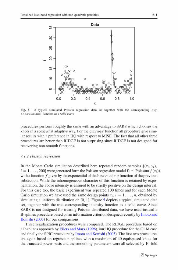
Data

Fig. 5 A typical simulated Poisson regression data set together with the corresponding exp(heavisine) function as a solid curve

procedures perform roughly the same with an advantage to SARS which chooses theknots in a somewhat adaptive way. For the corner function all procedure give simi-lar results with a preference in HQ with respect to MISE. The fact that all other threeprocedures are better than RIDGE is not surprising since RIDGE is not designed forrecovering non-smooth functions.

7.1.2 Poisson regression

In the Monte Carlo simulation described here repeated random samples {(xi , yi ),

i = 1, . . . , 200}were generated form the Poisson regression model Yi ∼ Poisson( f (xi )),with a function f given by the exponential of theheavisine function of the previoussubsection. While the inhomogeneous character of this function is retained by expo-nentiation, the above intensity is ensured to be strictly positive on the design interval.For this case too, the basic experiment was repeated 100 times and for each MonteCarlo simulation we have used the same design points xi , i = 1, . . . , n, obtained bysimulating a uniform distribution on [0, 1]. Figure 5 depicts a typical simulated dataset, together with the true corresponding intensity function as a solid curve. SinceSARS is not designed for treating Poisson distributed data, we have used instead aB-splines procedure based on an information criterion designed recently by Imoto andKonishi (2003) for our comparisons.

Three regularization procedures were compared. The RIDGE procedure based ona P-splines approach by Eilers and Marx (1996), our HQ procedure for the GLM caseand finally the SPIC procedure by Imoto and Konishi (2003). The first two proceduresare again based on regression splines with a maximum of 40 equispaced knots forthe truncated power basis and the smoothing parameters were all selected by 10-fold

123


0.0 0.2 0.4 0.6 0.8 1.0

510

2030

HQ

0.0 0.2 0.4 0.6 0.8 1.0

510

2030

RIDGE

0.0 0.2 0.4 0.6 0.8 1.0

510

2030

SPIC

RIDGE SPIC HQ

12

34

56

Intensity exp(Heavisine)

MS

E

BOXPLOTS

Fig. 6 Typical fits obtained with the various regularization procedures and the boxplots of their MSE over100 simulations

cross-validation. The SPIC procedure is based on B-splines with 30 knots and thesmoothing parameter for the Imoto and Konishi (2003) method is selected by theirSPIC-criterion.

In view of these simulations and the boxplots in Fig. 6 the HQ procedure has thesmallest MSE (due to a better tracking of the discontinuity and a less biased estimationof the small bump near to the point 0.64) followed by the RIDGE regression and theSPIC procedure. The RIDGE and SPIC procedures perform roughly the same, andseem to over-smooth the peak.

7.2 Analysis of real data

We illustrate our proposed procedure (HQ) through the analysis of the AIDS data(Stasinopoulos and Rigby 1992). This data set concerns the quarter yearly frequencycount of reported AIDS cases in the UK from January 1983 to September 1990 and isreproduced in Stasinopoulos and Rigby (1992). As suggested by these authors, afterdeseasonalising this time series, one suspects a break in the relationship between thenumber of AIDS cases and the time measured in quarter years.

We model the dependent variable Y (deseasonalised frequency of AIDS cases) by aPoisson distribution with mean a polynomial spline function of x , the time measuredin quarter years and have used the appropriate half quadratic procedure (HQ) with aspline basis based on 12 knots to fit the data. The deseasonalized data and the resultingfit, and the derivative of the fit are plotted in Fig. 7. One clearly sees a change in the

123


84 86 88 90

050

100

200

300

Time in quarter years

Num

ber

of A

IDS

cas

es

Fig. 7 Half Quadratic penalized fit (solid line) to the deseasonalized AIDS data. The dashed line is thederivative of the fitted regression curve

derivative at about July 1987. Stasinopoulos and Rigby (1992) suggested that thischange was caused by behavioral changes in high risk groups. See also Jandhyala andMacNeill (1997) for an analysis of these data.

Acknowledgments The authors are grateful to an Associate Editor and a reviewer for valuable commentsthat led to an improved presentation. Support from the IAP research network no. P6/03 of the Federal Sci-ence Policy, Belgium, is acknowledged. The second author also gratefully acknowledges financial supportby the GOA/07/04-project of the Research Fund KU Leuven.

References

Alliney, S., Ruzinsky, S. A. (1994). An algorithm for the minimization of mixed l1 and l2 norms withapplication to Bayesian estimation. IEEE Transactions on Signal Processing, 42, 618–627.

Antoniadis, A., Fan, J. (2001). Regularization of wavelets approximations (with discussion). Journal of theAmerican Statistical Association, 96, 939–967.

Belge, M., Kilmer, M. E., Miller, E. L. (2002). Efficient determination of multiple regularization parametersin a generalized L-curve approach. Inverse Problems, 18, 1161–1183.

Besag, J. E. (1989). Digital image processing: Towards Bayesian image analysis. Journal of AppliedStatistics, 16, 395–407.

Biller, C. (2000). Adaptive Bayesian regression splines in semiparametric generalized linear models.Journal of Computational and Graphical Statistics, 9, 122–140.

Black, M., Rangarajan, A. (1996). On the unification of line processes, outlier rejection, and robust statisticswith applications to early vision. International Journal of Computer Vision, 19, 57–91.

Ciarlet, P. G. (1989). Introduction to numerical linear algebra and optimisation. Cambridge Texts in AppliedMathematics. New York: Cambridge University Press.

Cox, D. D., O’Sullivan, F. (1990). Asymptotic analysis of penalized likelihood and related estimators. TheAnnals of Statistics, 18, 1676–1695.

de Boor, C. (1978). A practical guide to splines. New York: Springer.Delanay, A. H., Bressler, Y. (1998). Globally convergent edge-presering regularized reconstruction: An

application to limited-angle tomography. IEEE Transactions on Image Processing, 7, 204–221.Demoment, G. (1989). Image-reconstruction and restoration—overview of common estimation structures

and problems. IEEE Transactions on Acoustics Speech and Signal Processing, 37, 2024–2036.Denison, D. G. T., Mallick, B. K., Smith, A. F. M. (1998). Automatic Bayesian curve fitting. Journal of the

Royal Statistical Society, Series B, 60, 333–350.Dierckx, P. (1993). Curve and surface fitting with splines. Oxford Monographs on Numerical Analysis.

New York: Oxford University Press.DiMatteo, I., Genovese, C. R., Kass, R. E. (2001). Bayesian curve-fitting with free-knot splines. Biometrika,

88, 1055–1071.

123


Donoho, D., Johnstone, I., Hoch, J., Stern, A. (1992). Maximum entropy and the nearly black object. Journalof the Royal Statistical Society, Series B, 52, 41–81.

Donoho, D. L., Johnstone, I. M. (1994). Ideal spatial adaptation by wavelet shrinkage. Biometrika, 81,425–455.

Donoho, D. L., Johnstone, I. M. (1995). Adapting to unknown smoothness via wavelet shrinkage. Journalof the American Statistical Association, 90, 1200–1224.

Durand, S., Nikolova, M. (2006a). Stability of the minimizers of least squares with a non-convex regulari-zation. Part I: Local behavior. Applied Mathematics and Optimization, 53, 185–208.

Durand, S., Nikolova, M. (2006b). Stability of the minimizers of least squares with a non-convex regulari-zation. Part II: Global behavior. Applied Mathematics and Optimization, 53, 259–277.

Eilers, P. C., Marx, B. D. (1996). Flexible smoothing with B-splines and penalties (with discussion).Statistical Science, 11, 89–121.

Fahrmeir, L., Kaufman, H. (1985). Consistency of the maximum likelihood estimator in generalized linearmodels. The Annals of Statistics, 13, 342–368.

Fahrmeir, L., Tutz, G. (1994). Multivariate statistical modelling based on generalized linear models.Springer Series in Statistics. New York: Springer.

Fan, J. (1997). Comments on “Wavelets in statistics: A Review”, by A. Antoniadis. Journal of the ItalianStatistical Society, 6, 131–138.

Fan, J., Li, R. (2001). Variable selection via nonconcave penalized likelihood and its oracle properties.Journal of the American Statistical Association, 96, 1348–1360.

Fan, J., Peng, H. (2004). Nonconcave penalized likelihood with a diverging number of parameters. TheAnnals of Statistics, 32, 928–961.

Frank, I. E., Friedman, J. H. (1993). A statistical view of some chemometric regression tools (with discus-sion). Technometrics, 35, 109–148.

Friedman, J. H. (1991). Multivariate adaptive regression splines. The Annals of Statistics, 19, 1–67.Friedman, J. H., Silverman, B. W. (1989). Flexible parsimonious smoothing and additive modeling.

Technometrics, 31, 3–21.Fu, W. J. (1998). Penalized regressions: The bridge versus the Lasso. Journal of Computational and

Graphical Statistics, 7, 397–416.Geman, S., Geman, D. (1984). Stochastic relaxation, Gibbs distribution and the Bayesian restoration of

images. IEEE Transactions on Pattern Analysis and Machine Intelligenced, 6, 721–741.Geman, S., McClure, D. E. (1987). Statistical methods for tomographic image reconstruction. In

Proceedings of the 46-th session of the ISI, Bulletin of the ISI, 52, 22–26.Geman, D., Reynolds, G. (1992). Constrained restoration and the recovery of discontinuities. IEEE

Transactions on Pattern Analysis and Machine Intelligence, 14, 367–383.Geman, D., Yang, C. (1995). Nonlinear image recovery with half-quadratic regularization. IEEE

Transactions on Image Processing, 4, 932–946.Good, I. J., Gaskins, R. A. (1971). Nonparametric roughness penalities for probability densities. Biometrika,

58, 255–277.Green, P. J., Yandell, B. (1985). Semi-parametric generalized linear models. In R. Gilchrist, B. J. Francis,

J. Whittaker (Eds.), Generalized linear models, Vol. 32. Lecture notes in statistics (pp. 44–55). Berlin:Springer.

Gu, C., Kim, Y. J. (2002). Penalized likelihood regression: General formulation and efficient approximation.The Canadian Journal of Statistics, 30, 619–628.

Gu, C., Qiu, C. F. (1994). Penalized likelihood regression—a simple asymptotic analysis. Statistica Sinica,4, 297–304.

Gullikson, M., Wedin, P.-A. (1998). Analyzing the nonlinear L-curve. Technical Report, Sweden:Department of Computer Science, University of Umeøa.

Hastie, T. J., Tibshirani, R. J. (1990). Generalized additive models. Monographs on Statistics and AppliedProbability. New York: Chapman and Hall.

Hubert, P. J. (1967). The behavior of maximum likelihood estimates under nonstandard conditions. InProceedings of the Fifth Berkeley Symposium on Mathematical Statistics and Probability, 1, 221–233.

Imoto, S., Konishi, S. (2003). Selection of smoothing parameters in B-spline nonparametricregression models using information criteria. The Annals of the Institute of Statistical Mathematics,55, 671–687.

Jandhyala, V. K., MacNeill, I. B. (1997). Iterated partial sum sequences of regression residuals and testsfor changepoints with continuity constraints. Journal of the Royal Statistical Society, Series B, 59,147–156.

123


Klinger, A. (2001). Inference in high-dimensional generalized linear models based on soft-thresholding.Journal of the Royal Statistical Society, Series B, 63, 377–392.

Knight, K., Fu, W. (2000). Asymptotics for Lasso-type estimators. The Annals of Statistics, 28, 1356–1378.Lindstrom, M. J. (1999). Penalized estimation of free-knot splines Journal of Computational and Graphical

Statistics, 8, 333–352.Mammen, E., Van de Geer, S. (1997). Locally adaptive regression splines. The Annals of Statistics, 25,

387–413.McCullagh, P., Nelder, J. A. (1989). Generalized linear models, 2nd edn. London: Chapman & Hall.Nikolova, M. (2000). Local strong homogeneity of a regularized estimator. SIAM Journal of Applied

Mathematics, 61, 633–658.Nikolova, M. (2004). Weakly constrained minimization. Application to the estimation of images and signals

involving constant regions. Journal of Mathematical Imaging and Vision, 21, 155–175.Nikolova, M. (2005). Analysis of the recovery of edges in images and signals by minimizing nonconvex

regularized least-squares. SIAM Journal on Multiscale Modeling and Simulation, 4, 960–991.Nikolova, M., Ng, M. K. (2005). Analysis of half-quadratic minimization methods for signal and image

recovery. SIAM Journal on Scientific Computing, 27, 937–966.O’Sullivan, F. (1986). A statistical perspective on ill-posed inverse problems (with discussion). Statistical

Science, 1, 505–527.O’Sullivan, F., Yandell, B. S., Raynor, W. J. (1986). Automatic smoothing of regression functions in gen-

eralized linear models. Journal of the American Statistical Association, 81, 96–103.Park, M. Y., Hastie, T. (2007). L1-regularization path algorithm for generalized linear models. Journal of

the Royal Statistical Society, Series B, 69, 659–677.Poggio, T. (1985). Early vision: From computational structure to algorithms and parallel hardware.

Computer Vision, Graphics, and Image Processing, 31, 139–155.Rockafellar, R. T. (1970). Convex analysis. New Jersy: Princeton University Press.Rockafellar, T., Wets, R. J.-B. (1997). Variational analysis. Mathematics. Berlin: Springer.Ruppert, D., Carroll, R. (1997). Penalized regression splines. Working paper, School of Operations Research

and Industrial Engineering, Cornell University. Available at http://www.orie.cornell.edu/~davidr/papers.

Ruppert, D., Carroll, R. J. (2000). Spatially-adaptive penalties for spline fitting. Australian and New ZealandJournal of Statistics, 42, 205–223.

Stasinopoulos, D. M., Rigby, R. A. (1992). Detecting break points in generalized linear models.Computational Statistics & Data Analysis, 13, 461–471.

Stone, C. J., Hansen, M. H., Kooperberg, C., Truong, Y. K. (1997). Polynomial splines and their tensorproducts in extended linear modeling. The Annals of Statistics, 25, 1371–1470.

Tibshirani, R. J. (1996). Regression shrinkage and selection via the Lasso. Journal of the Royal StatisticalSociety, Series B, 58, 267–288.

Tikhonov, A. N. (1963). Solution of incorrectly formulated problems and the regularization method. SovietMath Dokl, 4, 1035–1038. (English translation).

Tishler, A., Zang, I. (1981). A new maximum likelihood algorithm for piecewise regression. Journal of theAmerican Statistical Association, 76, 980–987.

Titterington, D. M. (1985). Common structure of smoothing techniques in statistics. International StatisticalReview, 53, 141–170.

Whittaker, E. (1923). On a new method of graduation. Proceedings of Edinburgh Mathematical Society,41, 63–75.

Yu, Y., Ruppert, D. (2002). Penalized spline estimation for partially linear single-index models. Journal ofthe American Statistical Association, 97, 1042–1054.

Yuan, M., Lin, Y. (2007). On the non-negative garrotte estimator. Journal of the Royal Statistical Society,Series B, 69, 143–161.

Zhao, P., Yu, B. (2006). On model selection consistency of Lasso. Journal of Machine Learning Research,7, 2541–2563.

Zhou, S., Shen, X. (2001). Spatially adaptive regression splines and accurate knot selection schemes. Journalof the American Statistical Association, 96, 247–259.

Zou, H. (2006). The adaptive Lasso and its oracle properties. Journal of the American Statistical Association,101, 1418–1429.

123

http://www.orie.cornell.edu/~davidr/papers

http://www.orie.cornell.edu/~davidr/papers

Penalized likelihood regression for generalized linear models with non-quadratic penalties

Documents

Transcript of Penalized likelihood regression for generalized linear models with non-quadratic penalties