Metabolic network analysis Marcin Imielinski University of Pennsylvania March 14, 2007.
59
Metabolic network analysis Marcin Imielinski University of Pennsylvania March 14, 2007
-
date post
19-Dec-2015 -
Category
Documents
-
view
213 -
download
0
Transcript of Metabolic network analysis Marcin Imielinski University of Pennsylvania March 14, 2007.
Metabolic network analysis
Marcin Imielinski
University of Pennsylvania
March 14, 2007
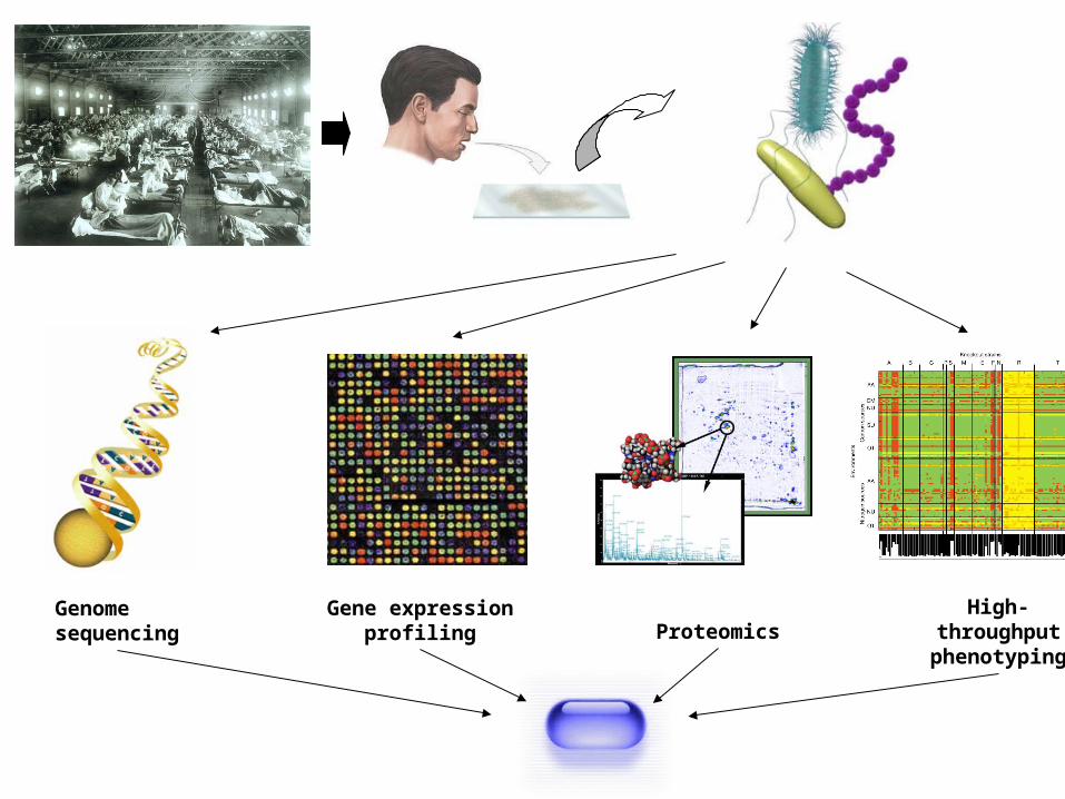
Genome sequencing
Gene expression profiling Proteomics
High-throughput phenotyping

The systems biology vision.
Integrate quantitative and high-throughput experimental data to gain insight into basic biology and pathophysiology of cells, tissues, and organisms.
Exploit knowledge of intracellular networks for drug design.
Engineer organisms, e.g. for salvaging waste, synthesizing fuel.
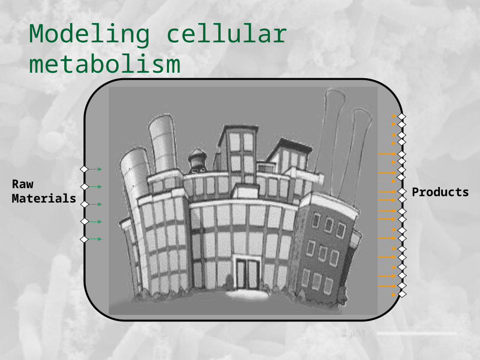
Modeling cellular metabolism
Raw Materials Products
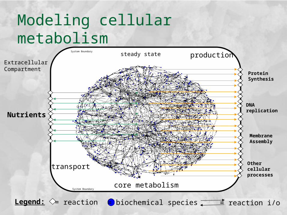
ExtracellularCompartment
System Boundary
System Boundary
production
transport
core metabolism
steady state
Other cellularprocesses
Modeling cellular metabolism
Legend: = reaction = biochemical species = reaction i/o
Nutrients
Protein Synthesis
DNA replication
MembraneAssembly
Glucose
Pyruvate
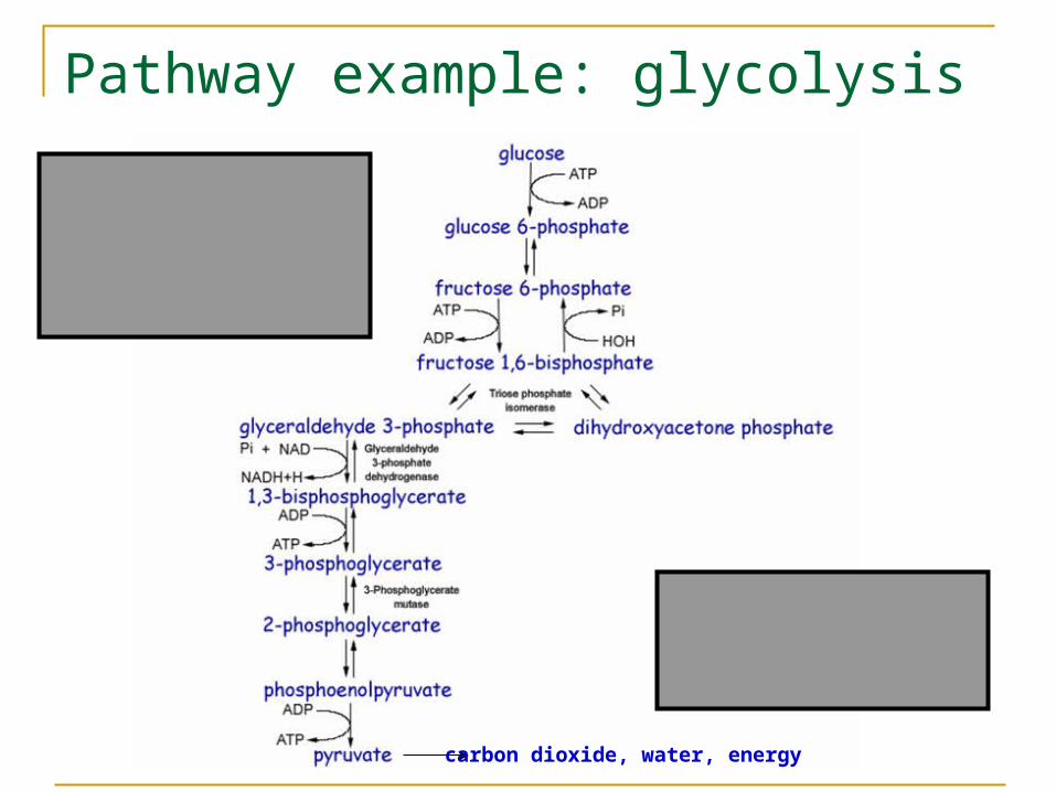
Pathway example: glycolysis
carbon dioxide, water, energy

Genome scale metabolic models Most comprehensive summary of the current knowledge
regarding the genetics and biochemistry of an organism Integrate functional genomic associations between genes,
proteins, and reactions into single model Models have been built for 100+ bacterial organisms, yeast,
human mitochondrion, liver cell, et al. Average model contains 500-1500 reactions and 300 – 1000
biochemical species.
SequencedGenome
FunctionalAnnotations
Predicted Genes and
Proteins
GenomeScaleModel
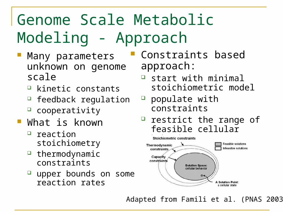
Genome Scale Metabolic Modeling - Approach Many parameters
unknown on genome scale kinetic constants feedback regulation cooperativity
What is known reaction stoichiometry thermodynamic
constraints upper bounds on some
reaction rates
Constraints based approach: start with minimal
stoichiometric model populate with constraints restrict the range of feasible
cellular behavior
Adapted from Famili et al. (PNAS 2003)
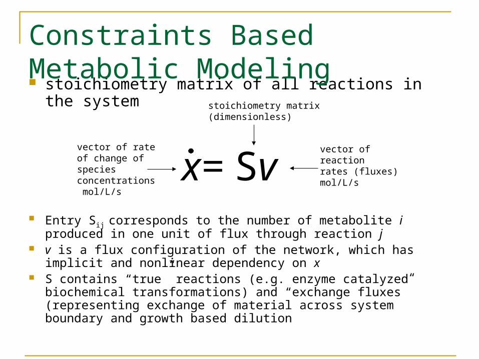
stoichiometry matrix of all reactions in the system
Entry Sij corresponds to the number of metabolite i produced in one unit of flux through reaction j
v is a flux configuration of the network, which has implicit and nonlinear dependency on x
S contains “true” reactions (e.g. enzyme catalyzed biochemical transformations) and “exchange fluxes” (representing exchange of material across system boundary and growth based dilution
x= Sv
Constraints Based Metabolic Modeling
stoichiometry matrix (dimensionless)
vector of rate of change of species concentrations mol/L/s
vector of reactionrates (fluxes)mol/L/s
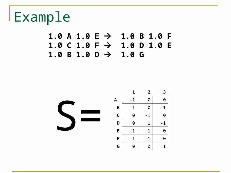
Example
S=
1.0 A 1.0 E 1.0 B 1.0 F 1.0 C 1.0 F 1.0 D 1.0 E 1.0 B 1.0 D 1.0 G
1 2 3
A -1 0 0
B 1 0 -1
C 0 -1 0
D 0 1 -1
E -1 1 0
F 1 -1 0
G 0 0 1

Example
S=1 2 3
A -1 0 0
B 1 0 -1
C 0 -1 0
D 0 1 -1
E -1 1 0
F 1 -1 0
G 0 0 1
systemboundary
1
2
3biochemical species
reaction
reaction I/O
Legend

Example
1 2 3
A -1 0 0
B 1 0 -1
C 0 -1 0
D 0 1 -1
E -1 1 0
F 1 -1 0
G 0 0 1
systemboundary
1
2
3
= xv
biochemical species
reaction
reaction I/O
Legend
Example – flux configuration
1 2 3
A -1 0 0
B 1 0 -1
C 0 -1 0
D 0 1 -1
E -1 1 0
F 1 -1 0
G 0 0 1
systemboundary
1
2
3
= 1
0
0
-1
1
0
0
-1
1
0
steady state species
consumed species
produced species
reaction (inactive)
reaction I/O
Legend
reaction (active)

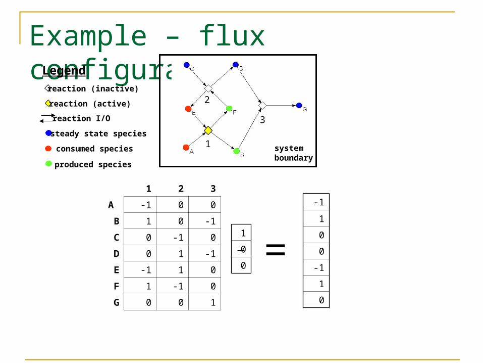
Example – flux configuration
1 2 3
A -1 0 0
B 1 0 -1
C 0 -1 0
D 0 1 -1
E -1 1 0
F 1 -1 0
G 0 0 1
systemboundary
1
2
3
= 1
1
0
-1
1
-1
1
0
0
0
steady state species
consumed species
produced species
reaction (inactive)
reaction I/O
Legend
reaction (active)
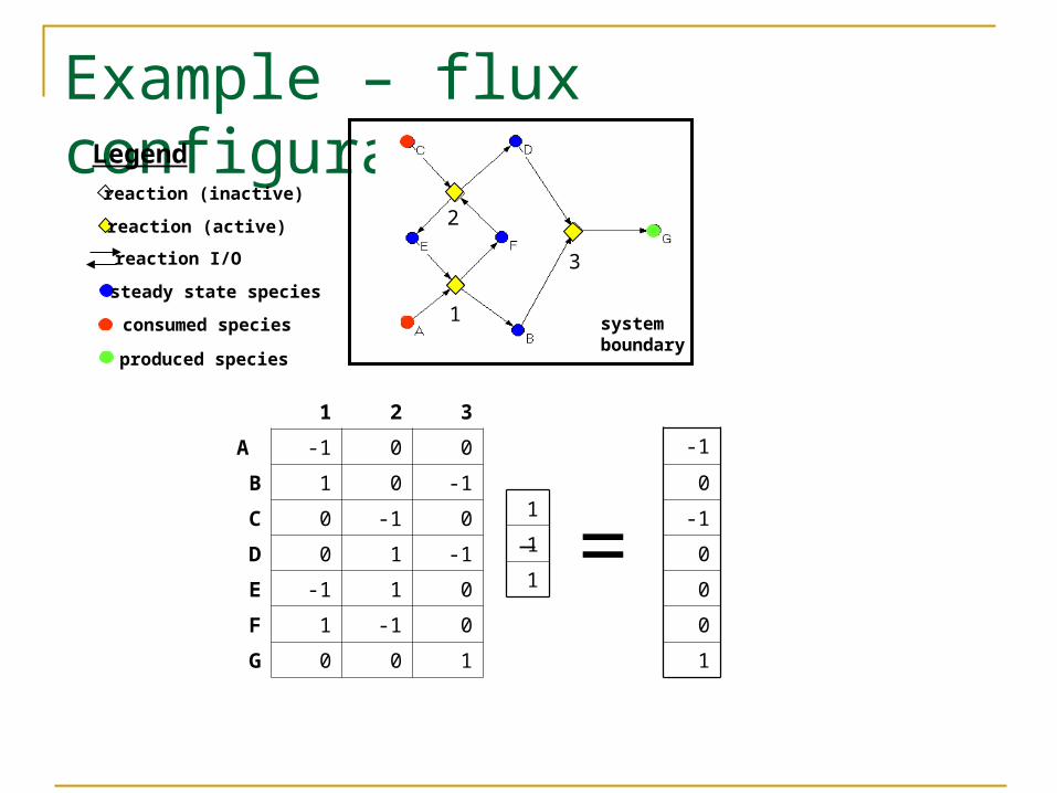
Example – flux configuration
1 2 3
A -1 0 0
B 1 0 -1
C 0 -1 0
D 0 1 -1
E -1 1 0
F 1 -1 0
G 0 0 1
systemboundary
1
2
3
= 1
1
1
-1
0
-1
0
0
0
1
steady state species
consumed species
produced species
reaction (inactive)
reaction I/O
Legend
reaction (active)

Constraints Based Metabolic Modeling stoichiometry matrix of all reactions in the
system quasi-steady state assumption
biochemical reactions are fast with respect to regulatory and environmental changes
stoichiometry matrix (dimensionless)
vector of rate of change of species concentrations mol/L/s
vector of reactionrates (fluxes)mol/L/s

Example – steady state
1 2 3
A -1 0 0
B 1 0 -1
C 0 -1 0
D 0 1 -1
E -1 1 0
F 1 -1 0
G 0 0 1
systemboundary
1
2
3
= 0v
biochemical species
reaction
reaction I/O
Legend

Example – steady state
1 2 3
A -1 0 0
B 1 0 -1
C 0 -1 0
D 0 1 -1
E -1 1 0
F 1 -1 0
G 0 0 1
systemboundary
1
2
3
= 00
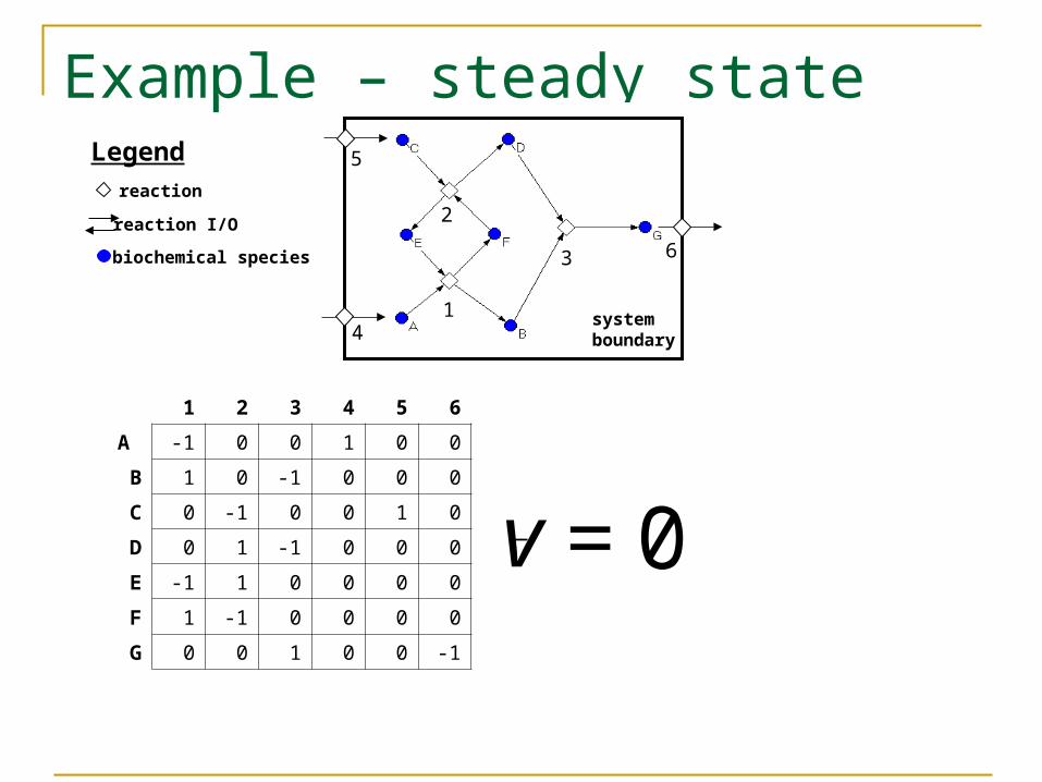
Example – steady state
1 2 3 4 5 6
A -1 0 0 1 0 0
B 1 0 -1 0 0 0
C 0 -1 0 0 1 0
D 0 1 -1 0 0 0
E -1 1 0 0 0 0
F 1 -1 0 0 0 0
G 0 0 1 0 0 -1
systemboundary
1
2
3
5
4
6
= 0v
biochemical species
reaction
reaction I/O
Legend

Example – steady state
1 2 3 4 5 6
A -1 0 0 1 0 0
B 1 0 -1 0 0 0
C 0 -1 0 0 1 0
D 0 1 -1 0 0 0
E -1 1 0 0 0 0
F 1 -1 0 0 0 0
G 0 0 1 0 0 -1
systemboundary
1
2
3
= 1
1
1
1
1
1
0
0
0
0
0
0
0
5
4
6
steady state species
consumed species
produced species
reaction (inactive)
reaction I/O
Legend
reaction (active)

Example – expanded system boundary
1 2 3 4 5 6
A -1 0 0 1 0 0
B 1 0 -1 0 0 0
C 0 -1 0 0 1 0
D 0 1 -1 0 0 0
E -1 1 0 0 0 0
F 1 -1 0 0 0 0
G 0 0 1 0 0 -1
Aext 0 0 0 -1 0 0
Cext 0 0 0 0 -1 0
Gext 0 0 0 0 0 1
oldsystemboundary
1
2
3
= 1
1
1
1
1
1
0
0
0
0
0
0
0
-1
-1
1
4
5
6
Cext
Aext
Gext
expandedsystemboundary
steady state species
consumed species
produced species
reaction (inactive)
reaction I/O
Legend
reaction (active)

Constraints Based Metabolic Modeling
stoichiometry matrix (dimensionless)
vector of rate of change of species concentrations mol/L/s
vector of reactionrates (fluxes)mol/L/s
stoichiometry matrix of all reactions in the system
quasi-steady state assumption irreversibility constraints
Irreversibilityconstraints

The Flux Cone
chull (p1, …, pq)
(extreme pathway decomposition)
(polyhedral flux cone)
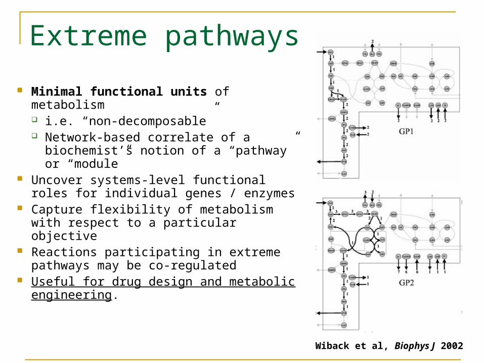
Minimal functional units of metabolism i.e. “non-decomposable” Network-based correlate of a
biochemist’s notion of a “pathway” or “module”
Uncover systems-level functional roles for individual genes / enzymes
Capture flexibility of metabolism with respect to a particular objective
Reactions participating in extreme pathways may be co-regulated
Useful for drug design and metabolic engineering.
Extreme pathways
Wiback et al, Biophys J 2002

1 2 3 4 5 6 7 8 9 10 11 12 13
Ru5P 0 0 -1 -2 0 1 0 0 0 0 0 1 2
FP2 0 -1 0 0 0 0 1 -1 0 0 1 0 0
F6P 1 0 0 2 0 0 -1 1 0 -1 0 0 -2
GAP 0 2 0 1 -1 0 0 0 0 0 -2 0 -1
R5P 0 0 1 -1 0 0 0 0 -1 0 0 -1 1
Extreme pathways: example
system boundary1 10
8
7
5 9
2
11
123
4
13
6
biochemical species
reaction
reaction I/O
Legend

system boundary1 10
8
7
5 9
2
11
123
4
13
6
1 2 3 4 5 6 7 8 9 10 11 12 13
Extreme pathway 1 1 1 0 0 2 0 1 0 0 0 0 0 0
Extreme pathway 2 0 0 1 0 0 1 0 0 1 0 0 0 0
Extreme pathway 3 0 0 1 1 1 3 0 0 0 2 0 0 0
Extreme pathway 4 0 0 2 2 0 6 0 1 0 5 1 0 0
Extreme pathway 5 0 2 1 1 5 3 2 0 0 0 0 0 0
Extreme pathway 6 5 1 4 0 0 0 1 0 6 0 0 0 2
Extreme pathways: example
biochemical species
reaction
reaction I/O
Legend

1 2 3 4 5 6 7 8 9 10 11 12 13
Extreme pathway 1 1 1 0 0 2 0 1 0 0 0 0 0 0
Extreme pathway 2 0 0 1 0 0 1 0 0 1 0 0 0 0
Extreme pathway 3 0 0 1 1 1 3 0 0 0 2 0 0 0
Extreme pathway 4 0 0 2 2 0 6 0 1 0 5 1 0 0
Extreme pathway 5 0 2 1 1 5 3 2 0 0 0 0 0 0
Extreme pathway 6 5 1 4 0 0 0 1 0 6 0 0 0 2
Extreme pathways: example
system boundary1 10
8
7
5 9
2
11
123
4
13
6
biochemical species
reaction
reaction I/O
Legend

system boundary1 10
8
7
5 9
2
11
123
4
13
6
1 2 3 4 5 6 7 8 9 10 11 12 13
Extreme pathway 1 1 1 0 0 2 0 1 0 0 0 0 0 0
Extreme pathway 2 0 0 1 0 0 1 0 0 1 0 0 0 0
Extreme pathway 3 0 0 1 1 1 3 0 0 0 2 0 0 0
Extreme pathway 4 0 0 2 2 0 6 0 1 0 5 1 0 0
Extreme pathway 5 0 2 1 1 5 3 2 0 0 0 0 0 0
Extreme pathway 6 5 1 4 0 0 0 1 0 6 0 0 0 2
Extreme pathways: example
biochemical species
reaction
reaction I/O
Legend

1 2 3 4 5 6 7 8 9 10 11 12 13
Extreme pathway 1 1 1 0 0 2 0 1 0 0 0 0 0 0
Extreme pathway 2 0 0 1 0 0 1 0 0 1 0 0 0 0
Extreme pathway 3 0 0 1 1 1 3 0 0 0 2 0 0 0
Extreme pathway 4 0 0 2 2 0 6 0 1 0 5 1 0 0
Extreme pathway 5 0 2 1 1 5 3 2 0 0 0 0 0 0
Extreme pathway 6 5 1 4 0 0 0 1 0 6 0 0 0 2
Objective: disable output of GAP (“exchange reaction” 5)
system boundary1 10
8
7
5 9
2
11
123
4
13
6
biochemical species
reaction
reaction I/O
Legend
Knockout design

system boundary1 10
8
7
5 9
2
11
123
4
13
6
1 2 3 4 5 6 7 8 9 10 11 12 13
Extreme pathway 1 1 1 0 0 2 0 1 0 0 0 0 0 0
Extreme pathway 2 0 0 1 0 0 1 0 0 1 0 0 0 0
Extreme pathway 3 0 0 1 1 1 3 0 0 0 2 0 0 0
Extreme pathway 4 0 0 2 2 0 6 0 1 0 5 1 0 0
Extreme pathway 5 0 2 1 1 5 3 2 0 0 0 0 0 0
Extreme pathway 6 5 1 4 0 0 0 1 0 6 0 0 0 2
biochemical species
reaction
reaction I/O
Legend
Knockout design
One solution: knockout reactions 1 and 4 (i.e. constrain v1=0 and v4=0)

system boundary1 10
8
7
5 9
2
11
123
4
13
6
1 2 3 4 5 6 7 8 9 10 11 12 13
Extreme pathway 1 1 1 0 0 2 0 1 0 0 0 0 0 0
Extreme pathway 2 0 0 1 0 0 1 0 0 1 0 0 0 0
Extreme pathway 3 0 0 1 1 1 3 0 0 0 2 0 0 0
Extreme pathway 4 0 0 2 2 0 6 0 1 0 5 1 0 0
Extreme pathway 5 0 2 1 1 5 3 2 0 0 0 0 0 0
Extreme pathway 6 5 1 4 0 0 0 1 0 6 0 0 0 2
One solution: knockout reactions 1 and 4 (i.e. constrain v1=0 and v4=0)
biochemical species
reaction
reaction I/O
Legend
Knockout design

1 2 3 4 5 6 7 8 9 10 11 12 13
Extreme pathway 1 1 1 0 0 2 0 1 0 0 0 0 0 0
Extreme pathway 2 0 0 1 0 0 1 0 0 1 0 0 0 0
Extreme pathway 3 0 0 1 1 1 3 0 0 0 2 0 0 0
Extreme pathway 4 0 0 2 2 0 6 0 1 0 5 1 0 0
Extreme pathway 5 0 2 1 1 5 3 2 0 0 0 0 0 0
Extreme pathway 6 5 1 4 0 0 0 1 0 6 0 0 0 2
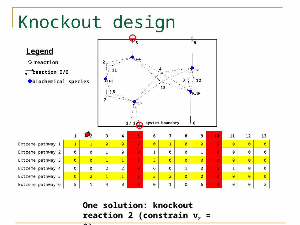
Objective: couple export of GAP to export of F6P
system boundary1 10
8
7
5 9
2
11
123
4
13
6
biochemical species
reaction
reaction I/O
Legend
Knockout design
1 2 3 4 5 6 7 8 9 10 11 12 13
Extreme pathway 1 1 1 0 0 2 0 1 0 0 0 0 0 0
Extreme pathway 2 0 0 1 0 0 1 0 0 1 0 0 0 0
Extreme pathway 3 0 0 1 1 1 3 0 0 0 2 0 0 0
Extreme pathway 4 0 0 2 2 0 6 0 1 0 5 1 0 0
Extreme pathway 5 0 2 1 1 5 3 2 0 0 0 0 0 0
Extreme pathway 6 5 1 4 0 0 0 1 0 6 0 0 0 2
system boundary1 10
8
7
5 9
2
11
123
4
13
6
One solution: knockout reaction 2 (constrain v2 = 0)
biochemical species
reaction
reaction I/O
Legend
Knockout design

Tableau algorithm for EP computatioon
Iteration 0: nonnegative orthant
Extreme rays of K0 = Euclidean basis vectors 1 … n
Iteration i+1:
Given
and extreme rays of Ki
Compute extreme rays of Ki+1

v1
v2
v3
Extreme ray of Ki
Tableau algorithm for EP computatioon

v1
v2
v3
Si+1v = 0
Tableau algorithm for EP computatioon

v1
v2
v3
Si+1v = 0
Sort extreme rays of Ki with regards to which are on (+) side, (-) side, and inside hyperplane Si+1v = 0
Tableau algorithm for EP computatioon

v1
v2
v3
Si+1v = 0
Extreme rays of Ki that are already in Siv=0 are automatically extreme rays of Ki+1
Tableau algorithm for EP computatioon

v1
v2
v3
Si+1v = 0
Combine pairs of extreme rays of Ki that are on opposite sides of Si+1v = 0
Tableau algorithm for EP computatioon

v1
v2
v3
Si+1v = 0
From this new ray collection remove rays that are non-extreme.
Tableau algorithm for EP computatioon

v1
v2
v3
Si+1v = 0
Non-extreme rays are r for which there exists an r* in the collection such that NZ(r*) is a subset of NZ(r)
Tableau algorithm for EP computatioon
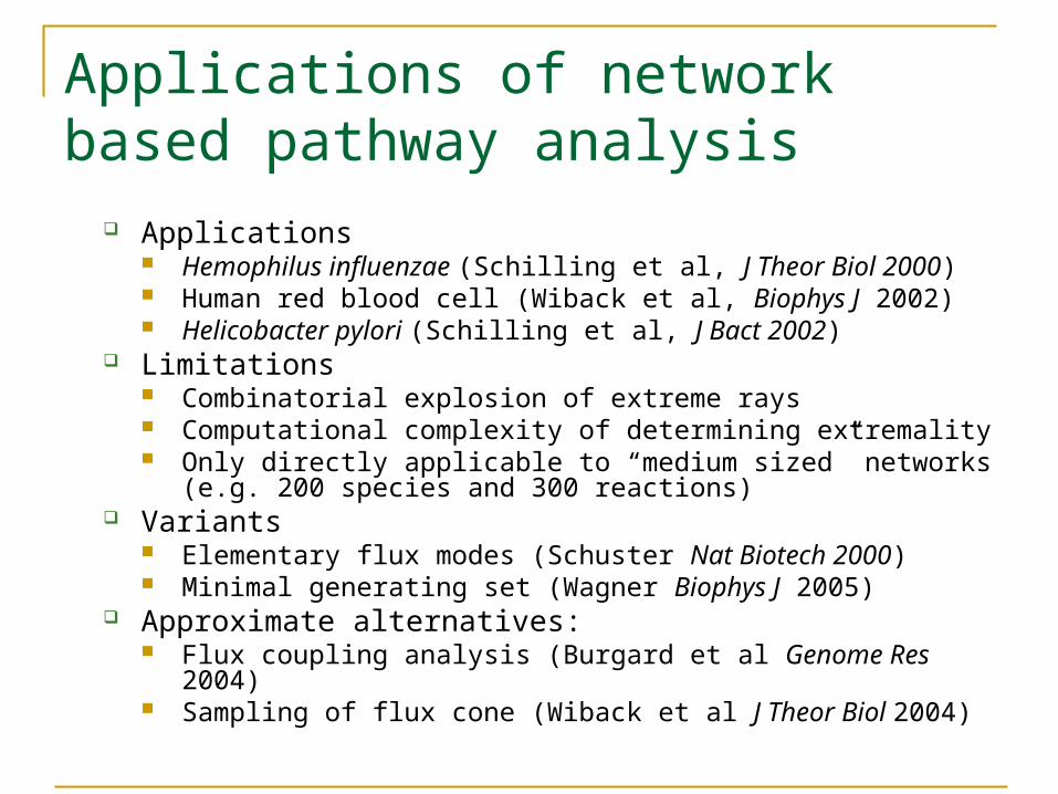
Applications Hemophilus influenzae (Schilling et al, J Theor Biol 2000) Human red blood cell (Wiback et al, Biophys J 2002) Helicobacter pylori (Schilling et al, J Bact 2002)
Limitations Combinatorial explosion of extreme rays Computational complexity of determining extremality Only directly applicable to “medium sized” networks (e.g. 200 species
and 300 reactions) Variants
Elementary flux modes (Schuster Nat Biotech 2000) Minimal generating set (Wagner Biophys J 2005)
Approximate alternatives: Flux coupling analysis (Burgard et al Genome Res 2004) Sampling of flux cone (Wiback et al J Theor Biol 2004)
Applications of network based pathway analysis

Flux Balance Analysis (Palsson et al.) Supplement metabolic
network with a “biomass reaction” which consumes biomass substrates in ratios specified by chemical composition analysis of the cell.
Model growth as flux through biomass reaction at steady state
Use linear programming to predict optimum growth under a given set of mutations and nutrient conditions.
Nu
trie
nts
Bio
ma
ss
Edwards et al Nat Biotech 2001
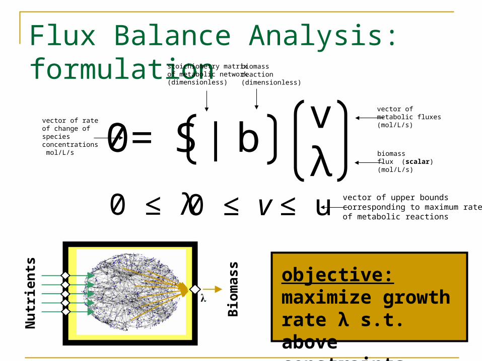
0 ≤ v ≤ u vector of upper boundscorresponding to maximum ratesof metabolic reactions
0= S | b
Flux Balance Analysis: formulationstoichiometry matrix
of metabolic network (dimensionless)
vector of rate of change of species concentrations mol/L/s
vector ofmetabolic fluxes (mol/L/s)
biomassreaction (dimensionless)
biomassflux (scalar)(mol/L/s)
objective: maximize growth rate λ s.t. above constraints
vλ
0 ≤ λ
Nu
trie
nts
Bio
ma
ss

Modeling E. coli growth using FBA (Edwards et al Nat Biotech 2001)
E coli model with 436 metabolites and 720 reactions
Found that in vivo growth matched FBA-predicted optimal growth on minimal nutrient media employing acetate and succinate as carbon sources.

Modeling E. coli growth using FBA (Ibarra et al Nature 2001)
In vivo growth was sub-optimal under glycerol
However following over 40 days of culture and 700 generations of cell divisions, E. coli adaptively evolved to achieve optimum predicted growth rate

Modeling E. coli mutants using FBA
Edwards et al 2004 E. coli model 436 species x 720 reactions compared FBA predictions to published data on 36 E. coli gene deletion
mutants in 4 nutrient media. 68 of 79 mutants agreed (qualitatively) between “simulation” and
experiment. Covert et al 2004 E. coli model 761 species x 931 reactions
Compared FBA predictions to 13,750 mutant growth experiments in different nutrient media – gene deletion combination
Found 78.7% agreement
Nu
trie
nts
Bio
ma
ss
0 ≤ v ≤ u
0= S | b
0 ≤ λ
vλ
maximize λ s.t.
ui=0

FBA: concerns and limitations Assumes that a cell culture is optimized for growth.
Even bacteria like to do other things than just grow. “Higher organisms” have even more complex “objectives”
Even if we allow that a wild type organism is optimized for growth (because of years of evolution) a mutant may have difficulty “finding” the global optimum. e.g. maybe a mutant bacteria will want to find the “closest” feasible
state. What about alternative optima?
Optimal manifolds of these LPs are high-dimensional polyhedral sets.
How will gene regulation influence the optimum? Simple version: regulation will alter the upper bound constraints (u)
on the fluxes. Complicated version: modeling the interaction of metabolism and
gene regulation will require including parameters and nonlinearities.

FBA: concerns and limitations Assumes that a cell culture is optimized for growth.
Even bacteria like to do other things than just grow. “Higher organisms” have even more complex “objectives”
Even if we allow that a wild type organism is optimized for growth (because of years of evolution) a mutant may have difficulty “finding” the global optimum. e.g. maybe a mutant bacteria will want to find the “closest”
feasible state. What about alternative optima?
Optimal manifolds of these LPs are high-dimensional polyhedral sets.
How will gene regulation influence the optimum? Simple version: regulation will alter the upper bound constraints (u)
on the fluxes. Complicated version: modeling the interaction of metabolism and
gene regulation will require including parameters and nonlinearities.

Minimization of metabolic adjustment (MOMA)Segre et al PNAS 2002 Alternative method to FBA
for computing mutant growth rates.
Hypothesize that mutants will want to settle “close” to the wild type flux configuration.
Find mutant flux distribution v that minimizes Euclidean distance to wild type growth state vwt
Formulate as QP vwt can be obtained
experimentally or computed using FBA.
Segre et al PNAS 2002

Regulatory on-off minimization (ROOM)Shlomi et al PNAS 2005 Also hypothesize that mutants
will want to be “close” to wild type flux configuration.
However measure distance as the number of reactions whose flux bounds would have to be (significantly) changed from wild type
Formulated as a MILP, with objective to minimize the number of reactions that need to be changed from wild type vwt (obtained using FBA).
Performance on test data set of mutants: ROOM > FBA >> MOMA (ROOM has fewer false negatives)
Shlomi et al PNAS 2005
MO
MA
wt
(F
BA
)R
OO
M
“biomass”
“biomass”
“biomass”
Review
Stoichiometry matrix and constraints-based metabolic modeling
Extreme pathway analysis Flux balance analysis Variants on FBA: MOMA and ROOM

Other topics not covered today Incorporating gene regulation to FBA
Covert et al Nature 2004 Analyzing alternative optima in FBA
Mahadevan et al Metab Eng 2003 Sampling the feasible flux region
Almaas et al Nature 2004 Wiback et al J Theor Biol 2004
Applying FBA to understand evolution Papp et al Nature 2004 Pal et al Nat Genetics 2005
Modeling thermodynamic constraints Beard et al J Theor Biol 2004 Qian et al Biophys Chem 2005
Conservation laws in metabolic networks Famili et al Biophys J 2003 Imielinski et al Biophys J 2006