Mercury: the planet and its orbitewilcots/courses/.../mercury.pdf · Introduction ... Mercury is...

INSTITUTE OF PHYSICS PUBLISHING REPORTS ON PROGRESS IN PHYSICS

Rep. Prog. Phys. 65 (2002) 529–560 PII: S0034-4885(02)12697-2

Mercury: the planet and its orbit

Andre Balogh and Giacomo Giampieri

Space and Atmospheric Physics, Imperial College, London SW7 2BW, UK

E-mail: [email protected]

Received 7 August 2001, in final form 26 November 2001Published 20 March 2002Online at stacks.iop.org/RoPP/65/529

Abstract

The planet closest to the Sun, Mercury, is the subject of renewed attention among planetaryscientists, as two major space missions will visit it within the next decade. These will bethe first to return to Mercury, after the flybys by NASA’s Mariner 10 spacecraft in 1974–5.The difficulties of observing this planet from the Earth make such missions necessary forfurther progress in understanding its origin, evolution and present state. This review providesan overview of what is known about Mercury and what are the major outstanding issues.Mercury’s orbital and rotation periods are in a unique 2:3 resonance; an analysis of the orbitaldynamics of Mercury is presented here, as well as Mercury’s special role in testing theoriesof gravitation. These derivations provide a good insight into the complexities of planetarymotion in general, and how, in the case of Mercury, its proximity to the Sun can be describedand exploited in terms of general relativity. Mercury’s surface, superficially similar to that ofthe Moon, presents intriguing differences, representing a different, and more complex historyin which the role of early volcanism remains to be clarified and understood. Mercury’s interiorpresents the most important puzzles: it has the highest uncompressed density among theterrestrial planets, implying a very large, mostly iron core. This does not appear to be thecompletely solidified yet, as Mariner 10 found a planetary magnetic field that is probablygenerated by an internal dynamo, in a liquid outer layer of the large iron core. The currentstate of the core, once established, will provide a constraint for its evolution from the timeof the planet’s formation. Mercury’s environment is highly variable. There is only a tenuousexosphere around Mercury; its source is not well understood, although there are competingmodels for its formation and dynamics. The planetary magnetic field appears to be strongenough to form a magnetosphere around the planet, through its interaction with the solar wind.This magnetosphere may have similarities with that of the Earth, but is more likely to bedominated by global dynamics that could make it collapse at least at the time of large solaroutbursts. The future understanding of the planet will now await the arrival of the new spacemissions. The review concludes with a brief description of these missions.

0034-4885/02/040529+32$90.00 © 2002 IOP Publishing Ltd Printed in the UK 529

http://stacks.iop.org/rp/65/529

530 A Balogh and G Giampieri

Contents

Page1. Introduction 5312. Orbital motion and spin–orbit coupling 534

2.1. History of observations and their interpretation 5342.2. Librations 5362.3. Tidal effects 5382.4. Cassini’s laws 5392.5. Gravity field of Mercury 540

3. A laboratory for relativistic physics 5414. Mercury’s surface 5445. Mercury’s interior, evolution and magnetic field 5496. Mercury’s environment: the exosphere and the magnetosphere 5527. Conclusions and the forthcoming space missions to Mercury 555

Acknowledgments 558References 559

Mercury 531

1. Introduction

The planet Mercury has been known since antiquity when it was observed, together with Venus,Mars, Jupiter and Saturn, as an object that moved against the background of the ‘motionless’star patterns. It is remarkable that it became so well known, despite its proximity to the settingor rising Sun, moving much faster across the pattern of the stars than the other planets. Itbecame known as the swift one, the messenger of the gods.

Mercury is the planet closest to the Sun in our solar system and is a member of the familyof terrestrial planets. Its generally Moon-like appearance is illustrated in figure 1, a compositeof over 140 photos taken by the only spacecraft ever to visit Mercury in 1974–5. The mainproperties of Mercury are listed in table 1, together with the same parameters for the Earth toprovide a comparison.

For planetary astronomers of modern times, the difficulties of observing Mercury haveled to its relative neglect. Earth-based astronomical observations of Mercury have alwaysbeen highly problematic. The planet’s largest apparent angular distance from the Sun is only28◦, so that it can only ever be observed close to sunset or sunrise, low above the horizon.This introduces severe limitations to viewing the planet because of atmospheric turbulence.Although its orbit and size were well established in the 19th century, the puzzle of the advancein its perihelion could not be explained by even the most careful observations and calculationswithin the framework of the Newtonian theory of gravitation; it awaited the advent of Einstein’sgeneral relativity (GR) for a solution. Even its rotational period was unknown or, rather,incorrectly deduced from the observations until the 1960s. As a consequence, the resonancebetween its orbital and rotational periods remained misinterpreted until that time.

For a long time, it was thought that Mercury’s rotation and orbit were in a 1:1 resonance,just like the Moon in its orbit around the Earth. As described in section 2, the orbital period of87.969 days introduces a near periodicity in favourable viewing conditions from the Earth thatleads to the same aspect of Mercury to be observed on successive occasions. This somewhatunfortunate coincidence affecting the visual observations was only resolved when, eventually,Mercury’s rotation period was found to be 58.646 days by Earth-based radar observations(Pettengill and Dyce 1965). This discovery showed that the orbital and rotation periods are infact in an exact 2:3 ratio.

The explanation for this resonant but asynchronous rotation of Mercury was first putforward by Colombo (1965). Further work on understanding the details of the resonance andthe libration of Mercury’s orbit in terms of spin–orbit coupling and tidal effects in Mercury’sliquid core led to important constraints on the evolution and state of the planet. This topicis developed in detail in section 2. Although the calculations are relatively lengthy, a logicaldevelopment of the arguments provides a good insight into the complexity of the interplay offorces that lead to the close coupling between Mercury’s orbital motion and rotation.

For physicists, Mercury’s importance stems from its role in the possibility to test, andindeed prove, the departure from the Newtonian theory of gravitation. It is generally knownthat the minute advance in Mercury’s perihelion (43 arcsec per century) that cannot be explainedby Newtonian gravitation has been successfully explained by GR. The details of the calculationsin the context of relativistic metric theories of gravitation are critically summarized in section 3.

The angular diameter of Mercury from the Earth is 13 arcsec at its maximum, and canbe as small as 4.5 arcsec. The small size, combined with the difficult observation conditions,led to a variety of features on the surface that were apparently deduced from astronomicalobservations, but then discarded. In fact, all the maps of Mercury’s main surface featuresdrawn by successive observers were proved to be wrong when close-up images of the planetwere finally returned by the Mariner 10 spacecraft in 1974–5. The observations made during


Figure 1. This mosaic shows the planet Mercury as seen by Mariner 10 as it sped away from theplanet on March 29, 1974. The mosaic was made from over 140 individual frames taken about 2 hafter encounter, at a range of 60 000 km. North is at top. The limb is at right, as is the illuminatingsunlight. The equator crosses the planet about two-thirds of the way from the top of the disc.The terminator, line-separating day from night, is about 190◦ west longitude. This hemisphere isdominated by smooth plains, rather than heavily cratered terrain, and resembles portions of theMoon’s maria in general shape. Half of a very large, multi-ringed basin named the Caloris Basinappears near the centre of the disc near the terminator. Its surrounding mountain ring is about1300 km in diameter (courtesy of NASA).

the three flybys of Mercury by this spacecraft remain by far the most important source ofinformation for the planet. Even Earth-orbiting, space-based telescopes, such as the HubbleSpace Telescope, cannot contribute to the study of Mercury, because the planet’s angularproximity to the Sun would lead to the violation of stray-light and thermal constraints of thetelescopes. However, some Earth-based spectroscopic studies, as well as radar observations,have contributed significant elements to our current knowledge of Mercury since the Mariner10 mission. Pioneering observations from the Earth since the Mariner 10 flybys did discoverthe variability of the sodium exosphere and also gave few important clues about the previouslyunseen side and polar regions of the planet. It now seems certain that there are volatiles, mostlikely water ice in deep craters near the poles. A particular radar feature on the side of theplanet not seen by Mariner 10 has been tentatively interpreted as a volcanic dome, although thisinterpretation remains subject to doubt. What is known of Mercury’s surface, primarily basedon the images made of it by Mariner 10 but complemented by radar and infrared observationsfrom Earth made under difficult conditions, is described in section 4.

Mariner 10’s flybys provided not only images of about 46% of the planet’s surface but alsoled to the discovery of the planetary magnetic field (Ness et al 1974, 1975). This discovery, inturn, led to an important re-evaluation of our understanding of Mercury’s formation, evolutionand present state. Before Mariner 10, it was thought that Mercury’s planetary core hadcompletely solidified early in the planet’s history, in fact within the first 500 million years

Mercury 533

Table 1. A summary of the main properties of Mercury compared to the Earth.

Mercury Earth

Bulk quantities

Mass µ (1024 kg) 0.3302 5.9736Equatorial radius R (km) 2439.7 6378.1Gµ (106 km3 s−2) 0.022 03 0.3986J2 (10−6) 60 1083C22 (10−6) 10 1.57

Orbital parameters

Semimajor axis(106 km) 57.91 149.60Orbital period (days) 87.969 365.256Synodic period (days) 115.88 —Sidereal rotation period (h) 1407.6 23.9345Length of day (h) 4222.6 24.00Orbital eccentricity 0.2056 0.0167Orbital inclination (deg.) 7.00 0.00Longitude of perihelion (deg.) 77.46 102.95Longitude of ascending node (deg.) 48.33 348.74Obliquity to orbit (deg.) ∼0.1 23.45

of its now ∼4.5 billion year existence. However, a planetary scale magnetic field implies thepossibility of a planetary dynamo, similar to that of the Earth; this, in turn, requires that at leastthe outer part of the core should have remained liquid to the present day. Given that Mercury’smostly iron core occupies a much greater volume of the planet than is the case for the Earth,its internal structure and how it evolved to its present state remain little understood. Recentmodelling, however, have provided some intriguing pointers that will be reviewed in section 5,together with their implications for the generation of the internal magnetic field.

Mercury has no stable atmosphere, but only a very tenuous exosphere; this is due to theplanet’s proximity to the Sun, its small size and mass (and therefore low surface gravity) andthe very high temperature of its dayside surface. The planetary magnetic field is strong enoughto create a magnetosphere, the cavity that results from the interaction of the magnetic field withthe solar wind. Although this magnetosphere has similarities to the Earth’s magnetosphere, thedifferences are both quantitative and qualitative. Its size, relative to the planet, is much smallerthan that of the Earth’s; this leads to considerable differences in the time constants and scalesizes of the plasma processes. Additionally, the absence of a stable atmosphere at Mercuryand, consequently, the absence of a conductive ionospheric layer above the planet, means thatit is unclear how the electrical currents that are involved in the formation and dynamics of themagnetosphere are closed around Mercury. It is evident that magnetospheric phenomena atMercury have more intimate relationship with the planet and in particular its surface than inthe case of the Earth. The magnetospheric models that are based on the important but limitedobservations by Mariner 10 are reviewed and discussed in section 6.

A significant difficulty in learning more about Mercury, even in the space age, is thelocation of the planet, deep in the gravitational well of the Sun. A considerable amount ofenergy is needed to reach it with a spacecraft launched from Earth, and a further large amountis required to place the spacecraft into orbit around Mercury. As a result, no space missionhas visited Mercury since the pioneering flybys of Mariner 10. An additional difficulty forspace missions to Mercury is the very hostile thermal environment of the planet. Not only isthe orbit close to the Sun: a practical consequence of the relatively slow rotation period and itsresonance with the orbital period is that a Mercury day (the period between two epochs when


the Sun is seen at zenith from the same point on the surface) is in fact two Mercury years, orabout 176 Earth-days. This means that its sunlit surface reaches very high temperatures (up tomore than 400 ◦C), while its nightside cools down considerably (to less than −100 ◦C).

However, two space missions are now under development, one by NASA and one, jointly,by the European Space Agency (ESA) and the Japan’s Institute of Space and AstronauticalSciences (ISAS). These two missions, described briefly in section 7, will place three orbitersaround Mercury, and even a small craft to land on the surface of the planet is being envisaged.It is expected that the range of observations that will be made by these space missions willbring, at the end of the decade, a significantly better understanding of most aspects of thisplanet.

The renewed interest in Mercury in the past years stems from the recognition that thehistory of the terrestrial planets, the Earth, Venus, Mars and Mercury itself, needs to beunderstood, as a whole, to make progress in understanding the formation of planetary systemsmore generally. These planets represent a unique family, a group of relatively small planetaryobjects, close to our star, the Sun; such planetary systems are unlikely to be discovered aroundother stars in the foreseeable future. All these planets have their own special histories, resultingin the apparently large differences that can be seen today; but Mercury is, among the terrestrialplanets, the least known and least understood of the family. The solar system remains, despitethe discovery of an increasing number of planetary objects around other stars, the true prototypeof a planetary system. It is the only one to which we have a direct access; indeed it is likely toremain for the foreseeable future the only planetary system that we can study and understandin detail as well as a whole.

2. Orbital motion and spin–orbit coupling

2.1. History of observations and their interpretation

Among the planets, Mercury is one of the most difficult to observe optically, due to its smallluminosity and especially to its proximity to the Sun. As a consequence, unreliable mapdrawings, and some preconceptions, led to wrong conclusions about the dynamical state of theplanet, which survived for almost a century.

At the end of 19th century, Schiaparelli (1889) made multiple observations of the planet.His tentative mapping of the planet’s surface allowed him to conclude that, in contrast toprevious speculations, Mercury is rotating very slowly, at a rate comparable to its orbital angularfrequency. More precisely, he claimed that the rotation period was exactly the same as theperiod of revolution of the planet around the Sun, i.e. that Mercury was locked in a synchronousstate. Schiaparelli’s conclusion was confirmed and supported by many other observers in thelast century (for a complete account of these observations and their interpretation, see Colomboand Shapiro (1966), Cruikshank and Chapman (1967), Chapman (1988)). One reason behindtheir mistake was probably that the most favourable conditions for observing the planet areseparated in time by three synodic periods, in addition to the fact that the rotation, orbital andsynodic periods are almost exactly in a 6:4:3 resonance (see figures 2 and 3). Thus, after thistime interval, the same features of the planetary surface appear to the observers to be almostexactly in the same place, and therefore assuming a synchronous state seemed a quite obviousinference. This wrong conclusion may be considered a rare case in science where the Occam’srazor argument can be misleading. After all, it would have taken an imaginative mind to guessthat the same set of observations could have been explained by a rotation state resonant butnot synchronous. It should also be reminded that another occurrence in our solar system of anon-synchronous spin–orbit coupling is yet to be found. Thus, this blunder survived until the

Mercury 535

0

12

3

4

5

6 6

7

8

9

1011

12S U N SUN

orbi t 1 orbit 2

Figure 2. Spin–orbit resonance. The arrow indicates the orientation of the long axis of Mercury.It takes two revolutions around the Sun to return to the original configuration in inertial space.

AU

-0.4 0.0 0.4 0.8

AU

-0.6

-0.4

-0.2

0.0

0.2

0.4

0.6

Sun

Earth

0

1

2

3

4

Figure 3. The path of Mercury with respect to the Sun–Earth reference direction. The solidcircles represents the position of the planet at one orbital period intervals. Since position ‘4’ isalmost coincident with the initial position ‘0’, we are in presence of an approximate 4:3 resonancebetween the orbital and synodic periods. This coincidence may explain the historical difficulty indetermining the planetary rotation rate, as described in the text.

mid 1960s, when radar observations (Pettengill and Dyce 1965) produced the first conclusiveevidence that Mercury is rotating three times on itself in exactly the time it takes to make tworevolutions around the Sun.

Figure 4 shows the apparent motion of the Sun, as seen in a reference frame centred onMercury and rotating with the planet’s spin rate. Note that it takes two revolutions to close thecurve. In the small loop at perihelion the orbital angular velocity becomes larger than the spinangular velocity, causing the Sun to move on a retrograde orbit for a short interval of time. Thisfact has important consequences for the long term effects of the tidal force from the Sun, asdiscussed below. Another peculiarity of Mercury’s orbit is that its eccentricity (e = 0.2056) isjust large enough to make this loop appear. Any eccentricity smaller than ∼0.20 would in factcause the Sun to slow down and then start again in the same direction, without any retrogradephase.


AU

-0.6 -0.4 -0.2 0.0 0.2 0.4 0.6

AU

-0.6

-0.4

-0.2

0.0

0.2

0.4

0.6

Mercury

Figure 4. The apparent motion of the Sun in a Mercury-fixed reference frame. The planet is at thecentre, with its long axis along the x-axis. Due to the spin–orbit resonance, the path is closed aftertwo revolutions. Small circles on the path corresponds to equal intervals of time. Note that duringa brief time interval at perihelion, the Sun’s apparent motion becomes retrograde.

2.2. Librations

Colombo (1965) and Colombo and Shapiro (1966) demonstrated how the rotation rate can beexactly 1.5 times the mean orbital angular frequency, as a result of a non-zero eccentricityand a small permanent asymmetry in the equatorial plane of the planet. Goldreich (1968) andGoldreich and Peale (1968) considered the problem of the probability of being captured in the3:2 resonance, as the planet is tidally despun.

Let us assume that Mercury’s spin axis is normal to its orbital plane, and that the principalmoments of inertia areA,B,C, withA < B < C, where C is the moment about the spin axis.The Sun exerts a torque along the spin axis, with magnitude

T = −3GM�2R3

p

(B − A) sin 2ψ (2.1)

where M� is the solar mass, Rp the Sun–Mercury distance, and ψ the angle between theplanet’s equatorial long axis and the direction to the Sun (see figure 5). From figure 5, therotation angle in inertial space is θ = f + ψ , where f is the true anomaly of the planet in itsorbit around the Sun.

The torque gives the rate of change of the spin angular momentum L

dL

dt= Cθ = T . (2.2)

Since Mercury’s spin is in a 3:2 resonance with the orbital angular frequency, we introducethe libration angle as

γ ≡ θ − 32M = ψ + f − 3

2M (2.3)

where M is the mean anomaly. From (2.1)–(2.3) we obtain

Cγ = −3

2

GM�R3p

(B − A) sin(2γ + 3M − 2f ). (2.4)

Mercury 537

f θ

ψ

Sun

Mercury

Referenceaxis

Figure 5. The geometry of the torque. Mercury’s long axis makes an angle θ with the inertialreference axis, and an angle ψ with the direction to the Sun. f = θ −ψ is the true anomaly of theplanet. Because of the resonance, the uniform rotation rate is θ ≈ 3

2n.

Table 2. Relevant eccentricity functions (from Kaula (2000)).

q G20q (e)

−2 0−1 −e/2 + e3/16 + · · ·

0 1 − 5e2/2 + 13e4/16 + · · ·+1 7e/2 − 123e3/16 + · · ·+2 17e2/2 − 115e4/6 + · · ·

Note that the factorR−3p in (2.4) is time dependent, due to the non-zero eccentricity of Mercury’s

orbit. We can replace it with the constant semiaxis a using (Kaula, 2000)(a

Rp

)3

sin(2γ + 3M − 2f ) =∑q

G20q(e) sin[2γ + (1 − q)M] (2.5)

where the G20q are functions of the eccentricity alone, and are listed in table 2.By using (2.5) in (2.4), and by replacing derivatives with respect to time with derivatives

with respect to M (indicated with a prime), we finally get

γ ′′ + α∑q

G20q(e) sin[2γ + (1 − q)M] = 0 (2.6)

where α ≡ 32B−AC

1.8 × 10−4. The equation for the long-term librations can be obtainedby averaging (2.6) over an orbital period, while holding γ ≈ const along a single orbit (sinceγ = θ − 3

2n 0 near resonance). The result is

γ ′′ + α G201(e) sin 2γ = 0. (2.7)

Equation (2.7) is a pendulum equation, the solution of which oscillates with a periodP (2αG201)

−1/2 revs 66 revs. We note from the expression of G201(e) given in table 2that, as first pointed out by Colombo (1965), e �= 0 is a necessary condition for the stabilityof the 3:2 resonance, as is the requirement that B �= A. Also, since G201(e) > 0, the stablelibrations are around γ ≈ 0, which means that the planet’s long axis points towards the Sun atperihelion.

Short period librations of frequency multiple of the orbital frequency can be studied byreplacing the appropriate expressions for G20q(e) in (2.6). In particular, the amplitude oflibrations with a periodicity equal to the orbital period is

�γ = α(G200 −G202) = 3

2

B − A

C

(1 − 11e2 +

959

48e4 + · · ·

) 20′′. (2.8)


Time (Mercury orbits)

0 1 2 3

γ (a

rcse

c)

-30

-20

-10

0

10

20

30

Figure 6. Short-term librations have the period of a Mercury year, and amplitude given by (2.8).

Other, shorter period librations are smaller than this by a factor O(e) or more, so that the 88 daylibration is indeed dominant. Figure 6 shows the periodic modulation of the libration angleover three orbital periods. Note that the short period librations, contrary to the long periodones, contain a forcing term, and do not damp to zero in presence of internal dissipation.

2.3. Tidal effects

So far, we have neglected the tidal effect of the Sun on the shape and internal mass distributionof Mercury. The tidal potential can be written as

Ut = Gµ

R

qt

3

( rR

)2 ( aR

)3P20(cos ζ ) (2.9)

where qt ≡ −3(M�/µ)(R/a)3 −1.4×10−6, and ζ is the angle between the observing pointand the direction to the Sun, measured from the centre of the planet. In order to determine theshape of the planet, the centrifugal force should also be taken into account. This force can bederived from the potential

Uc = −GµR

qr

3

( rR

)2[1 − P20(cosφ)] (2.10)

where qr ≡ θ2R3/Gµ = −3qt/4 10−6 and φ is the latitude. However, since the rotation isuniform, no periodic terms arise in the centrifugal potential, which can therefore be neglected.Thus, a point on the surface of the planet is subject to a periodic perturbing potential, whichto first order in e is given by

Up = Gµ

R

qt

12

[P22(sin φ) cos 2%

(cosM − e

2cos 2M

)−P22(sin φ) sin 2%

(sinM − e

2sin 2M

)− 6eP20(sin φ) cosM

](2.11)

where% is the longitude. Note that this periodic term does not goes to zero with the eccentricity.This is due to the fact that the Sun, as seen from a point on the planet’s surface, is not in a fixedposition, as, for example, the Earth is with respect to an observer on the Moon.

Thus, if Mercury is not perfectly rigid, a periodic modulation of the second-order gravityfield harmonics will be created by the tidal effect. By equating the perturbing potential tothe harmonic expansion of the gravitational potential (at the surface), these variations can beexpressed as a time dependent contribution to the second-order coefficients

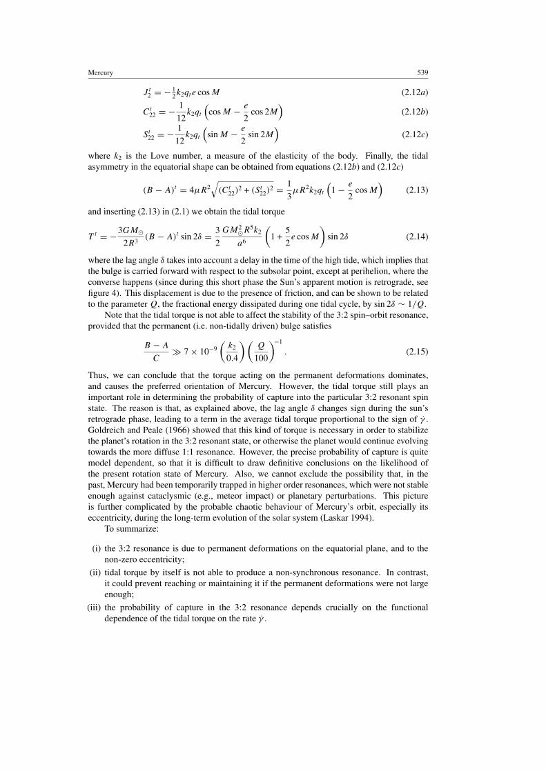
Mercury 539

J t2 = − 12k2qte cosM (2.12a)

Ct22 = − 1

12k2qt

(cosM − e

2cos 2M

)(2.12b)

St22 = − 1

12k2qt

(sinM − e

2sin 2M

)(2.12c)

where k2 is the Love number, a measure of the elasticity of the body. Finally, the tidalasymmetry in the equatorial shape can be obtained from equations (2.12b) and (2.12c)

(B − A)t = 4µR2√(Ct22)

2 + (St22)2 = 1

3µR2k2qt

(1 − e

2cosM

)(2.13)

and inserting (2.13) in (2.1) we obtain the tidal torque

T t = −3GM�2R3

(B − A)t sin 2δ = 3

2

GM2�R

5k2

a6

(1 +

5

2e cosM

)sin 2δ (2.14)

where the lag angle δ takes into account a delay in the time of the high tide, which implies thatthe bulge is carried forward with respect to the subsolar point, except at perihelion, where theconverse happens (since during this short phase the Sun’s apparent motion is retrograde, seefigure 4). This displacement is due to the presence of friction, and can be shown to be relatedto the parameter Q, the fractional energy dissipated during one tidal cycle, by sin 2δ ∼ 1/Q.

Note that the tidal torque is not able to affect the stability of the 3:2 spin–orbit resonance,provided that the permanent (i.e. non-tidally driven) bulge satisfies

B − A

C 7 × 10−9

(k2

0.4

) (Q

100

)−1

. (2.15)

Thus, we can conclude that the torque acting on the permanent deformations dominates,and causes the preferred orientation of Mercury. However, the tidal torque still plays animportant role in determining the probability of capture into the particular 3:2 resonant spinstate. The reason is that, as explained above, the lag angle δ changes sign during the sun’sretrograde phase, leading to a term in the average tidal torque proportional to the sign of γ .Goldreich and Peale (1966) showed that this kind of torque is necessary in order to stabilizethe planet’s rotation in the 3:2 resonant state, or otherwise the planet would continue evolvingtowards the more diffuse 1:1 resonance. However, the precise probability of capture is quitemodel dependent, so that it is difficult to draw definitive conclusions on the likelihood ofthe present rotation state of Mercury. Also, we cannot exclude the possibility that, in thepast, Mercury had been temporarily trapped in higher order resonances, which were not stableenough against cataclysmic (e.g., meteor impact) or planetary perturbations. This pictureis further complicated by the probable chaotic behaviour of Mercury’s orbit, especially itseccentricity, during the long-term evolution of the solar system (Laskar 1994).

To summarize:

(i) the 3:2 resonance is due to permanent deformations on the equatorial plane, and to thenon-zero eccentricity;

(ii) tidal torque by itself is not able to produce a non-synchronous resonance. In contrast,it could prevent reaching or maintaining it if the permanent deformations were not largeenough;

(iii) the probability of capture in the 3:2 resonance depends crucially on the functionaldependence of the tidal torque on the rate γ .


2.4. Cassini’s laws

In 1643 Cassini summarized the Moon’s rotational motion in three empirical laws:

(i) the rotation period is synchronous to the mean orbital period;(ii) the angle between the spin axis and the normal to the ecliptic is constant;

(iii) the spin axis, normal to the orbital plane, and normal to the ecliptic are always coplanar.

The first law is a consequence of tidal evolution, and, as we have seen, is also valid forMercury, provided that we replace the word ‘synchronous’ with ‘commensurate’. Colombo(1966) and Peale (1969) considered a generalization of the other two laws, by studying, ingeneral, the motion of the rotational axis of a rigid body subject to a gravitational torque.By making use of (2.2), written in a reference frame precessing with the orbital plane, it ispossible to show that the second and third laws are obtained as extremes in the energy of thesystem. Since the energy involves both the spin and orbital angular momenta, the minimizationis achieved through tidal interaction between the primary and the orbiting body. In particular,for the Mercury–Sun system there are three stable positions for the spin axis, and Mercury isgetting close to position 1, where the spin axis and the normal to the orbit are on the same sideof the normal to the ecliptic, and precessing around it at the same rate. Moreover, in general,the integral of the motion provides a relationship between the obliquity θ (the angle betweenthe spin axis and the normal to the orbital plane), and the moments of inertia factor (C−A)/A,with a small contribution from the quantity B − A due to the orbital resonance1. Thus, assuggested by Peale (1969), a measure of the obliquity of Mercury would provide a directmeasure of the factor (C−A)/C, with a small uncertainty related to the equatorial asymmetryB − A. When combined with the gravitational measurements of J2 (C − A)/µR2 andC22 = (B − A)/4µR2, this method would finally give the important quantity C/µR2.

In addition, Peale (1969) suggested combining the obliquity and gravitational fieldmeasurements, with that of the 88 day libration amplitude, given by (2.8), in order toobtain information about the nature of the liquid core. The basic assumption here is thatthe observed libration only refers to the mantle, provided that the latter is decoupled fromthe core. In other words, the factor C that appear in (2.8) should actually be replaced byCm, the mantle contribution to C. The other implicit assumption in Peale’s proposal is that(B − A)m ≈ (B − A), i.e. that the core is axially symmetric. Under this scheme, the ratioCm/C � 1 can be determined by combining the different measurements of gravity field,obliquity, and short-term librations.

2.5. Gravity field of Mercury

The third Mariner 10 flyby was designed at low altitude and without occultations, in order tobe able to determine the gravity field of the planet. Besides the mass, no other information wasavailable before then, and no other gravitational measurements could be made since. Thus,our knowledge of the gravitational field is still quite inaccurate, and can be summarized in thefollowing gravitational parameters (Anderson et al 1987), quoted in table 1:

Gµ = 22 032.09 ± 0.91 km3 s−2 (2.16a)

J2 = (6.0 ± 2.0)× 10−5 (2.16b)

C22 = (1.0 ± 0.5)× 10−5. (2.16c)

The measured value of J2 is considerably larger than its value in hydrostatic equilibrium, oforder qr ≈ 10−6, meaning that a large nonhydrostatic component is present, at least at the1 In other words, this additional term would disappear upon long-term averaging, if the rotational and orbital motionswere not commensurate.

Mercury 541

present epoch. Note that the gravitational measurements do not provide a direct measure ofthe moments of inertia, but only of their differences. For example, from the nonzero value ofC22, we can conclude that the equatorial moments of inertia are unequal, in agreement with thedynamical argument from section 2.2. In particular we find (B−A)/µR2 = 4C22 4×10−5.As far as the largest moment of inertia is concerned, differentiated models giveC 0.34µR2.Note that C = 0.4µR2 exactly for a Maclaurin spheroid of constant density. More generally,since the density decreases towards the surface, C is slightly smaller, and can be obtained fromthe Radau–Darwin relation and the knowledge of J2, if the planet is in hydrostatic equilibrium.In the case of Mercury, a non-hydrostatic planet, a dynamical measure of C is possible withthe method outlined in section 2.4, i.e. using the measured values of J2, C22 and obliquity.

3. A laboratory for relativistic physics

Thanks to its significant orbital eccentricity and proximity to the Sun, Mercury provides,through the study of its orbital motion, an excellent opportunity to test the theory of GR withinour solar system. Indeed, the relativistic perihelion precession (see below) represents one ofthe most famous classical tests of the theory, and the only one involving relativistic effects onmassive bodies—all other classical tests being based on light propagation effects only.

Since Mercury, as all solar system bodies, moves slowly (compared to the velocity oflight c) in a weak gravitational field, its motion can be accurately described by NewtonianPhysics. Relativistic effects amount just to small corrections to the classical keplerian elements.In the slow motion and weak field limit appropriate for describing the solar system’s dynamics,all metric theories of gravity, including GR and alternative relativistic theories, can be describedwithin a single theoretical framework, the so-called parametrized post-Newtonian (PPN)formalism. In the PPN formalism, all theories assume the same form, the only differencebetween them being in the values of a few PPN parameters (see Will (1993)). Basically,only two of such parameters, γ and β, appear in the equations of motion for Mercury. Theydescribe, respectively, the curvature of space–time produced by unit rest mass, and the amountof nonlinearity in the field equations. These two parameters are both equal to unity in GR,but can differ significantly in alternative theories of gravity, such as the Brans–Dicke theory.Other PPN parameters can be neglected, because of the small ratio2 µ/M� ∼ 2 × 10−7.

Using the PPN formalism, it can be shown (see, e.g., Will (1993)) that a body orbiting theSun is subject to a small perturbative acceleration given by (we take c = 1 hereafter)

δa = m�r3

[2(γ + β)

m�r

r− γ v2r + 2(γ + 1)(r · v)v

](3.1)

where m� ≡ GM�, r is the position vector of the body, and v its velocity. This accelerationacts in addition to the usual Newtonian term −m�r/r3. We indicate with R the componentof δa along the radial direction from the Sun, W the component normal to the orbital plane,and S the remaining component orthogonal to R and W . One finds, from (3.1)

R = m2�r3

[2β + γ

( ra

)+ 2(γ + 1)

(e2

1 − e2

) ( ra

)sin2 f

](3.2a)

S = m2�r3

[2(γ + 1)e sin f

](3.2b)

W = 0. (3.2c)

2 Moreover, these additional PPN parameters are exactly zero if the theory is required to be isotropic (no preferredframes in the Universe) and fully conservative (no violation of energy-momentum conservation).


The variation of the keplerian orbital elements (a, e, I,., ω, χ ≡ nt) can then be obtainedfrom the classical Lagrange’s variational equations (Roy 1982)

da

dt=

[4a3

m�(1 − e2)

]1/2

[Re sin f + S(1 + e cos f )] (3.3a)

de

dt=

[a(1 − e2)

m�

]1/2 [R sin f +

Se

(pr

− r

a

)](3.3b)

dI

dt= r

hW cos(ω + f ) (3.3c)

d.

dt= rW sin(ω + f )

h sin I(3.3d)

dω

dt=

[a(1 − e2)

m�e2

]1/2 [−R cos f + S 2 + e cos f

1 + e cos fsin f

]− d.

dtcos I (3.3e)

dχ

dt= − 1

na

[2r

a− 1 − e2

ecos f

]R − 1 − e2

nae

[1 +

r

p

]S sin f. (3.3f)

We can now integrate equations (3.3a)–(3.3f) to obtain the variations of the orbital elements,as function of time or true anomaly. A rather lengthy calculation gives

�a = − 2em�(1 − e2)2

[(2 + 3γ + 2β + (2 + γ )e2)� cos f − (2 + 2γ + β)e� sin2f ] (3.4a)

�e = − m�a(1 − e2)

[(γ + 2β + (4 + 3γ )e2)� cos f − (2 + 2γ + β)e� sin2f ] (3.4b)

�I = 0 (3.4c)

�. = 0 (3.4d)

�ω = m�a(1 − e2)

[(2 + 2γ − β)�f − (2 + 2γ + β)�(sin f cos f )

− (1 − e2)γ + 2β

e� sin f

](3.4e)

�M = m�a√

1 − e2

[(2 + 2γ + β)�(sin f cos f ) +

γ + 2β + (4 + 3γ )e2

e� sin f

]

− 3m�n�ta(1 − e2)2

[γ + β + (2 + γ )e2 + (2 + 3γ + 2β + (2 + γ )e2)e cos f0

+(2 + 2γ + β)e2 cos2 f0] − (2 + γ )

m�a�E (3.4f)

where the symbol � means the change in some quantity between the reference epoch (t0, f0)

and the present time t , and E is the eccentric anomaly.The four non constant orbital elements are shown in figure 7. Note that there is no long-

term effect on a and e, while the perihelion precesses secularly at the quite famous rate

ω = �ω(P )

P= 3m�na(1 − e2)c2

(2 + 2γ − β

3

)≈ 43′′ century−1. (3.5)

The relativistic precession corresponds to a displacement of the perihelion position of about29 km during one orbit. The existence of an anomalous precession of Mercury’s orbit has beenknown for a long time, since Le Verrier’s pioneering work in the 19th century. Newcomb (1882)reanalysed the recorded transits of Mercury, and concluded that ‘the discordance between theobserved and theoretical motions of the perihelion of Mercury, first pointed out by Le Verrier,

Mercury 543


0 1 2 3

∆M (

arcs

ecs)

-1.8

-1.2

-0.6

0.0

∆ω (

arcs

ecs)

-0.1

0.0

0.1

0.2

0.3

0.4

∆a (

km)

0

2

4

6

8

10


0 1 2 3

∆e (

x 10

7 )

0.0

0.5

1.0

1.5

2.0

Figure 7. Relativistic effect on orbital parameters a, e, ω,M . Note the secular trends in theargument of perihelion ω and mean anomaly M . The semiaxis a and eccentricity e show periodicperturbation of period of a Mercury year, and amplitude ∼9 km and 1.7 × 10−7, respectively.

really exists, and is indeed larger than he supposed . . . . It follows that the observed centennialmotion of the perihelion of Mercury is greater by 43′ than the theoretical motion computedfrom the best attainable values of the masses of the planets’. He even suggested that the lawof gravitation would need to be modified, e.g., by adding terms varying ‘as the inverse third orfourth power of the distance’.

The success of GR in explaining the orbital precession of Mercury has not been universallyaccepted without challenge, because of the presence of the solar quadrupole moment. In fact,it can be shown that the solar J2 also produces a secular precession of the orbit, at a rate

˙ω ≡ ω + . = 3J2R2�n

2a2(1 − e2)2

(2 − 5

2sin2I − cos I

)≈ 0.012′′

(J2

10−7

)century−1. (3.6)

Unfortunately, J2 of the Sun has never been directly measured. However, if the Sun isrotating as a rigid body, then J2 10−7, and therefore its effect on ˙ω would be negligible.Recent helioseismic measurements, along with the use of complex solar models, providedJ2 2 × 10−7 (Pijpers 1998), in good agreement with the rigid rotation hypothesis. It istherefore reasonable to assume that the contribution to ˙ω from J2 is marginal. Under thisassumption, extensive measurements of Mercury’s relativistic precession have indicated that(2 + 2γ − β)/3 ≈ 1, the value predicted by GR, with a precision of ∼0.3% (Anderson et al1991). In order to separately constrain β and γ , however, results from other relativistic testsneed to be taken into account (since, as stated above, classical tests based on light propagationeffects determine γ alone). Alternatively, one could try to measure the periodic effects on theorbital elements, as given by equations (3.4a)–(3.4f). This could be done by accurate radiotracking of a Mercury orbiter. An obvious advantage of the orbiter is that it could also providean independent and very accurate measure of the J2 of the Sun, through its effect on the nodalprecession . of the orbital plane, for which there is no relativistic counterpart. It is estimatedthat BepiColombo will provide J2 with a precision of a few parts in 109, which will lead to animprovement by two orders of magnitude in the measure of the relativistic parameters, alongwith a very significant constrain for solar interior models (Milani et al 2001b).

Finally, we mention that Mercury also represents an ideal environment for studying othersmall relativistic effects, such as (Will 1993, 2001, Anderson et al 1997):


(i) a time variation of the universal gravity constant G (the current upper limit on |G|/G is5 × 10−12 year−1).

(ii) Nordvedt violation of the strong equivalence principle (the parameter η which controlsthis effect is presently constrained to be |η| � 10−3).

(iii) de-Sitter geodetic precession (which causes Mercury’s orbital plane to precess at a rate∼0.2′′ year−1; so far, only the analogous effect on the Moon has been verified).

(iv) Gravitational redshift (currently tested with a precision 0.01%).

4. Mercury’s surface

Superficially Moon-like, Mercury’s surface is marked by cratering and (possibly) earlyvolcanism, evidence for early shaping and evolution of the surface features that have remainedunchanged over the past 3 or so billion years, in the absence of the kind of significant tectonicactivity that reshaped the surface of Venus and the Earth. Only about 46% of Mercury’s surfacewas imaged by Mariner 10, so that current conclusions concerning the formation and evolutionof the surface are awaiting the confirmation that only a complete imaging survey will be ableto bring. In fact, radar imaging of the unseen side of Mercury from Earth has provided atentative evidence of a large volcanic dome (Harmon 1997); no comparable features exist onthe side imaged by Mariner 10. This interpretation of the radar observations remains, however,uncertain; only the detailed imaging of the planet by he forthcoming space missions can resolvewhether Mercury’s unseen surface brings unexpected surprises as was the case with the Moon.

The Mariner 10 images have been extensively studied in order to establish the crateringhistory of the planet (Strom and Neukum 1988, Neukum et al 2001). The late heavybombardment (LHB) following the formation of the planets, between about 4.5 and 3.8 Ga(billion years) before the present, left Mercury’s surface marked by a distribution of craterssimilar to that of the Moon, but with a number of notable differences that have remained largelyunexplained, or at least could be explained by several alternative scenarios. A typical pictureof the Mercury surface is shown in figure 8, as photographed by Mariner 10; this pictureillustrates the cratered surface, as well as the transition to smoother, undulating plains. Theorigin of these intercrater plains, the most frequent type of terrain on Mercury, is uncertain,although they are generally considered to be of volcanic origin, rather than basin ejecta. Theirestimated age, 4.2–4 Ga, coincides with the period of LHB; the state of Mercury at that timewas likely to facilitate the widespread volcanism that would explain the age and spread of theintercrater plains (Spudis and Guest 1988). In this context, volcanism should be envisagedas the widespread flooding of the surface by subsurface, molten, volcanic lavas that emerged,rather than erupted, through the fractures in the relatively thin lithosphere. It is this process,rather than the more commonly understood formation of volcanoes and volcanic eruptions thatare likely to have formed the smooth plains on much of Mercury’s surface.

A good example, when comparing the cratering (and related) features of Mercury and theMoon, is the Caloris basin, if not the largest, the best-preserved and most complex impact-generated structure. Its diameter is about 1300 km, although only about half of it was imagedby Mariner 10. The Caloris basin is illustrated in figure 9. A strong similarity has been foundbetween the Caloris ring system and that of the Imbrium basin on the Moon; both have thesame morphology of six concentric rings, and both have smooth plains surrounding the mainbasin rim. It is this similarity that led to the suggestion that the smooth plains on Mercury,as the lunar maria, are of volcanic origin, in the sense described above, filling in the featuresleft by the impacts that led to the formation of the basins. The Caloris impact is consideredto be the most important such event in the history of Mercury. It was probably the last majorimpact, sufficiently violent to have led to widespread seismic activity and to the formation of

Mercury 545

Figure 8. This photograph of Mercury was taken by the Mariner 10 spacecraft from a range of55 340 km during the first Mercury encounter on March 29, 1974. It shows an area in the northernhemisphere, illustrating a transition from heavily cratered terrain to a smooth plain. These smoothplains areas on Mercury are thought to be volcanic in origin with lava flows filling in heavilycratered areas. The photograph area is about 490 km wide (courtesy of NASA).

the disturbed terrain on the opposite side of Mercury (see, e.g. Spudis and Guest (1988) andreferences within).

A particular feature of Mercury’s surface is the presence of lobate scarps that intersectpre-existing features, such as older craters. The lobate scarps have the form of elongatedridges of 1–2 km high and are thought to be thrust faults, evidence of tectonic activity andthe contraction of the planet, as its core cooled down. One of the most prominent examplesfound in the Mariner 10 observations is shown in figure 10. It is generally considered thatMercury’s radius was reduced by more than 1 km (estimates range from 1 to about 5 km) inthat process (Solomon 1977). Although tectonics have not played a major part in Mercury’shistory, signs of various tectonic activity, considered in the global history of the formation andevolution of the surface, provide important clues to the details of that history and also shedlight, if indirectly, on processes that occurred as the crust and mantle reached their presentstate (e.g. Thomas (1997)). The presence of a molten outer fraction of the core (see below)may mean that as the core is still cooling down, the process of contraction is continuing, albeiton geological timescales.

Mercury’s regolith is likely to be more mature than the Moon’s, with smaller grain sizesand a larger proportion of glassy particles (Langevin 1997) than that of the Moon. All theprocesses that are known in weathering planetary regoliths are likely to be more intense atMercury. These include solar radiation, occasionally impacting solar wind particles, solarenergetic particles; both the flux of solar photons and energetic particles is up to an order ofmagnitude higher than at the orbit of the Moon. As discussed in section 6 below, the existenceof the magnetosphere and the absence of an ionosphere imply that there must be electricalcurrents that may involve the surface layers of Mercury. The role played by the regolith inthese magnetospheric currents is unclear, but it may provide an important connection betweencharacteristics of the planetary surface and Mercury’s magnetosphere.

Earth-based radar studies have contributed in several ways to our knowledge of Mercury,beyond the crucial discovery of its rotational period, the consequences of which have alreadybeen discussed in detail. Radar has also been used to establish a range of topographicfeatures, as illustrated in figure 11. The discovery of the likely presence of volatiles, possibly


Figure 9. Mariner 10 image of part of the Caloris Basin. The floor is covered with smooth plains.Ridges form concentric rings around the centre of the basin (courtesy of NASA).

water ice, near the poles by ground-based radar observations is a remarkable result (Sladeet al 1992). Given the very small obliquity of Mercury (the axis of rotation is very nearlyperpendicular to the orbital plane, unlike for the Earth, see table 1), it was proposed thatsome of the craters near Mercury’s poles remain in permanent shadow and can retain volatilesdeposited in them by impacting comets. Radar images of the regions near the poles haveshown very bright features consistent with water ice; a detailed examination of the featureswas able to match the radar images with those craters that had been imaged by Mariner 10(Harmon et al 1994, Harmon 1997). It is not as yet excluded that other ices can also exist in thevery low temperatures (∼70 K) that have been estimated for the permanently shadowed portions

Mercury 547

Figure 10. One of the most prominent lobate scarps (Discovery Scarp), photographed by Mariner10 during its first encounter with Mercury, is located at the centre of this image (extending fromthe top to near bottom). This scarp is about 350 km long and transects two craters 35 and 55 kmin diameter. The maximum height of the scarp south of the 55 km crater is about 3 km. Notice theshallow older crater (near the centre of the image) perched on the crest of the scarp (courtesy ofNASA).

Figure 11. An illustration of the power of Earth-based radars for studying the topography ofMercury. These traces represent altimetric observations by the giant radio telescope/radar atArecibo, Puerto Rico, across the region south of the Caloris basin, dominated by undulationsin the smooth plains surrounding the basin. The indentation in the top trace represents the Mozartcrater (courtesy of J E Harmon, NAIC, Arecibo Observatory).

at the bottom of craters near the poles. The discovery of significant amounts of water ice inthe polar regions of the Moon (Feldman et al 1998) reinforces the interpretation of the radarobservations of Mercury, although the evidence for the interpretation of the radar data in termsof water ice comes primarily from the similarity of the radar scattering properties with thosefrom Jupiter’s icy satellites (Callisto, Europa and Ganymede) and from the martian ice caps. Itshould be noted, however, that there are no equivalent enhanced backscatter radar observationsfor the presence of water ice on the Moon where the evidence comes from measurements by theneutron spectrometer on the Lunar Prospector mission indicating a concentration of hydrogennear the polar regions (Feldman et al 2000).

Recent, high-resolution radar observations of Mercury’s polar regions have yieldedfurther detail on the locations of anomalous radar echoes and their possible explanations


(Harmon et al 2001). Given the improved resolution of these observations (at 1.5–3 kmbetter by a factor up to 10 than the earlier observations), the sources of the anomalous echoscould be located and studied in considerably greater detail. Generally speaking, the previousobservations have been confirmed; on the side imaged by Mariner 10 all the echoes could beidentified with specific craters, but, in addition, shadowing patterns within the craters couldbe distinguished. Furthermore, new features, at latitudes well away from the polar regions,have also been identified, implying the presence of water ice (or some other volatile) in cratersat latitudes as low as 75◦ as well as from craters of small (∼10 km) diameter. The presenceand survival of volatiles in such a wide range of locations implies their efficient retentionand protection that have not yet been fully explained. A range of possibilities remains thatonly further observations, allied with a better theoretical understanding and modelling of thescenarios that have been proposed for the retention of volatiles can resolve. A really crucialadditional information in this context would be the identification of the volatile(s) that causethe observed radar echos by new observations; while the general expectation is that suchobservations would confirm that it is water ice as implicitly assumed above, other, more exoticexplanations cannot at present be completely excluded (Harmon et al 2001).

The question whether lava flows formed the smooth plains is closely related to thegeochemical composition of Mercury’s surface and its evolution; the composition, however, isonly very poorly known. Some of the Mariner 10 images were re-analysed by Robinson andLucey (1997), using two recalibrated spectral channels of the Mariner 10 camera, in an attemptto determine compositional differences on the surface that could be related to topographicalfeatures. They were able to establish that there was a likely difference in the compositionof the minerals around the crater they studied (Rudaki) that corresponded to surface featuresthat could be attributed to lava flows. Similarly, a larger crater, Homer (320 km in diameter)has apparent compositional differences around it that are consistent with volcanic activity,also supported by the absence of impact features. Despite the very thorough analysis ofthe available evidence provided by these pictures, the conclusions concerning lava flows andvolcanic activity remain tentative.

Another way to study Mercury’s surface composition is provided by infrared andmicrowave observations made from Earth. All such observations are made under very difficultconditions, with generally poor spatial resolution, which make the conclusions highly tentative;however, until detailed imaging becomes available from the forthcoming space missions, itis these ground-based observations that provide the only new evidence concerning Mercury’ssurface composition. Jeanloz et al (1995) found strong evidence for the absence of basalt onMercury’s surface; this is significant because elsewhere on the terrestrial planets basalt is themost important material indicating the state of differentiation between the planets’ core andmantle. The conclusion drawn from this finding, the absence of extrusive volcanism, may alsoimply that the heat loss from the interior that would occur through volcanism did not occur inthe case of Mercury and contributed to retaining a hot interior for the planet.

Mid-infrared observations (Sprague et al 1997, 2000) have also provided information onthe presence of varieties of plagioclase feldspar on the surface of Mercury, and indications ofpyroxene. A considerable amount of effort has been made to compare lunar spectra and labora-tory spectra of different compositions to those obtained from Mercury’s surface. The objectiveof this research is to document the surface composition in as great detail as is possible from theseground-based observations, with a view to establish constraints on the evolution of Mercury’ssurface and the internal and external processes that led to its present state. The conclusionthat Mercury is a highly differentiated planet appears to be well established, with significantdifferences found between the Moon and Mercury in terms of the detailed composition of thesurface, although the processes that led to this differentiation remain poorly understood.

Mercury 549

Despite the remarkable progress made in understanding Mercury’s surface from the morethan 2500 images taken during the three Mariner 10 flybys, the limits of that venerablearchive have now probably been reached, although the new and sophisticated image processingtechniques used by Robinson and Lucey (1997) have led to some interesting, if very tentativeresults concerning the classification of the Mercury surface features. The limitations of theresolution in the images, as well as the absence of spectroscopic discrimination constrain theconclusions that can be reached. Similarly limited by resolution, ground-based infrared andmicrowave observations continue nevertheless to provide new information on the compositionof Mercury’s surface and its similarities and differences with the lunar surface, in particular.The new space missions, with their ambitious imaging capabilities, as well their multispectralresolution, will bring the definitive opportunity to settle the major outstanding issues.Complemented by geochemical probing using γ ray detectors, as well as UV and IR images,a comprehensive study of Mercury’s surface and its history can be undertaken. This widerange of observables will, of course, be complemented by complete coverage of Mercury’ssurface, much of it with overlapping images, and at least a significant fraction under differentconditions of solar illumination.

5. Mercury’s interior, evolution and magnetic field

The most striking feature of Mercury’s interior, its very large iron core, is deduced fromthe density of the planet. Figure 12 illustrates the point, showing the significantly largeruncompressed density of Mercury, when compared to those of the other terrestrial planets andthe Moon. A simple, two-component model of the interior gives the radius of the core as about0.75 of the radius of the planet, compared to 0.49 for Venus, 0.54 for the Earth and 0.44 forMars, as illustrated in figure 13. The composition of Mercury is also anomalous, since thedensity implies an iron/silicon ratio about twice that of the other terrestrial planets. The stateof the interior is not known; however, the discovery of the planetary magnetic field by Mariner10 opened up the possibility that at least the outer part of the core is still molten, to providethe dynamo mechanism for the generation of the magnetic field. This is contrary to what hadbeen expected prior to Mariner 10 and has led to an increasingly sophisticated modelling of thethermal evolution of the planet (Schubert et al 1988, Spohn et al 2001) to explain the currentstate of the interior.

The existence of the large core, mostly of iron, is not in doubt. It is also generally acceptedthat, shortly after its formation, the core was liquid. Before Mariner 10’s flybys, it was thoughtthat as the planet cooled, its mantle and crust formed and, due to its small size, the coolingrate should have solidified the core probably as early as 500 million years after its formation,assuming an iron core. However, if the magnetic field is generated by a still functioning internaldynamo (as in the case of the Earth) then the core cannot be completely solid, as dynamo theoryrequires a convecting and rotating liquid layer in the outer core. The only way, apparently,to delay the expected solidification of the core is to assume a small fraction of sulphur mixedwith the iron to form a eutectic alloy with a much lower melting temperature. This is quite areasonable assumption, as there were such volatiles present at the time of the formation of theterrestrial planets.

If sulphur is indeed present, even a small amount will lead to the formation a molten layerat the core–mantle boundary where the temperature is likely to exceed that of the eutecticof the iron–sulphur system. It is still unclear what fraction of sulphur is likely to be presentin Mercury and hence the likely thickness of the molten outer fraction in Mercury’s core isunknown, although it must be capable to generate the observed internal magnetic field. Thereare several reasons for this uncertainty. As examined recently by Harder and Schubert (2001),


Radius (km)

0 2000 4000 6000

Den

sity

(g.

cm-3

)

2

3

4

5

6

MERCURY

EARTH

VENUS

MARS

MOON

Figure 12. The uncompressed densities of the terrestrial planets and the Moon plotted againsttheir radii. Although no simple functional relationship is claimed by this figure, despite theapparent linearity for four of the objects, Mercury’s density does appear to be quite anomalouswhen compared to that of the other terrestrial bodies. It should be noted, however, that a physicallybased curve of mean density versus radius for constant composition would show that the Moon isas anomalous as Mercury.

M e r c u r y V e n u s Ear th M a r s

Figure 13. The four terrestrial planets and their cores, to scale. The size of Mercury’s core isinferred from its large density, and is calculated assuming a mostly iron core and a silicate mantle.

Mercury’s interior, in particular the exact size of the core is really unconstrained by our currentknowledge of Mercury (although we know that it is a large fraction of the radius). The gravityprobing that was discussed in detail in section 2 is essential for further progress, in particularthe precise measurements of the moment of inertia of the planet. The amount of sulphur inMercury’s core is also unknown. One of the related and quite fundamental problems is theformation of the planet (Cameron et al 1988). The question whether Mercury was formed atits present distance from the Sun is an important one, as the theories that provide models forthe early solar nebula, its composition, density and temperature distribution depend on ourunderstanding of the formation of the terrestrial planets and their evolution to their presentstate. The concentration of volatiles, such as sulphur (the key to Mercury’s internal structure),at the time of the formation of the planets is an important consequence of the scenarios that canbe envisaged for the solar nebula and the formation of Mercury (Lewis 1988). An additionalpossibility for the current state of Mercury (with its very high density and large core) is acatastrophic impact that removed a large part of the outer, silicate shell, leaving the alreadyformed core with a much thinner mantle (Wetherill 1988).

In the absence of sufficient data on Mercury’s gravitational field, the planetary scalemagnetic field provides the strongest constraint on Mercury’s interior. It is relatively weak,

Mercury 551

Figure 14. The correlation between the magnetic dipole and quadrupole moments of Mercury,determined from different analyses of the Mariner 10 flyby data (after Connerney and Ness (1988)and references therein). The different determinations cannot independently yield these two terms,but provide different values under different assumptions concerning the location of the dipole andthe interpretation of magnetospheric models.

with a dipole moment of about 300 nTR3. Energy considerations of the strength of the dynamo,based on the current interior models (Spohn et al 2001), imply a larger magnetic field, maybe byas much as an order of magnitude or more. Although some care must be exercised in interpretingthis conclusion, it is clear that Mercury’s internal structure is not sufficiently constrained, noris the hydrodynamic dynamo sufficiently well understood to explain the limited Mariner 10observations. One of the limitations of the Mariner 10 data set is that spatial aliasing, inherentto the limited measurements made along the flyby trajectory of the spacecraft, makes theinterpretation of the structure of the magnetic field ambiguous. In particular, it is not possible todistinguish uniquely the relative magnitudes of the dipole and quadrupole terms of the planetaryfield (Connerney and Ness 1988). The different interpretations of the observations, dependenton assumptions concerning, in particular, the contribution of magnetospheric currents (seebelow), is illustrated in figure 14 (after Connerney and Ness (1988)).

It is clear that the constraints on Mercury’s interior models need to be reinforced bymore comprehensive measurements of both the magnetic field and of the gravitational field ofMercury. A full mapping of the magnetic field is required, to derive not only the dipole andquadrupole terms, but also the higher order terms which are needed for discriminating betweenthe possible models of the origin of Mercury’s internal magnetic field. Given the likelihoodthat Mercury’s magnetic field originates in either the outer layers of its core or at the core–mantle boundary, such a field should produce measurable higher order terms (e.g., the modelproposed for a thermoelectric dynamo, Stevenson (1987)). The modelling of the measurementsperformed on simple current systems in Mercury’s interior (Giampieri and Balogh 2001a)indicates that the presence of the magnetosphere and its current systems will affect theaccuracy with which the internal terms can be determined, even by an orbiting spacecraft.


However, further modelling has shown that magnetic field measurements to be made onthe more closely circular orbit of the BepiColombo Planetary Orbiter are likely to yieldthe coefficients of the magnetic field to order 10 or higher. This, together with the gravityfield measurements, will allow identifying the conditions at the core–mantle boundary, andexamining the possible operation of the thermoelectric dynamo (Spohn et al 2001, Giampieriand Balogh 2001b).

As explained in great details in section 2, quantitative constraints on Mercury’s internalstructure will come from the determination of the lower order terms of the spherical harmonicexpansion of its gravitational potential (Spohn et al 2001, Milani et al 2001a). Particularlyuseful will be monitoring the periodic modulation of the gravitational harmonics, given byequations (2.12a)–(2.12c), which will provide a measure of the Love number k2. This numberis defined as the ratio between the time-dependent deformation of the gravitational potentialof the planet and the external potential that leads to the deformation; in effect, it measures thetidal response to the solar gravitational potential. Modelling the Love number will yield, inturn, constraints on the thickness of the fluid layer of the core and to estimates of the viscosityof the mantle. The higher orders of the gravitational potential will provide information on theinhomogeneities in the mass distribution of the mantle as well as the likely non-uniformitiesat the core–mantle interface (Milani et al 2001a).

6. Mercury’s environment: the exosphere and the magnetosphere

There is no stable atmosphere around Mercury, unlike around the other terrestrial planets. Inthat respect, Mercury is similar to the Moon, just as there is a strong similarity between theirsurface features. There is, however, a tenuous exosphere, in which the constituent atoms havevery large mean free paths; densities are low and highly variable. The total column densityis probably less than 1012 cm−2. The existence of three elements, O, H, He, was establishedduring the Mariner 10 flybys; the presence of Na, K and Ca was detected by ground-basedobservations. Other elements, such as Al, Fe, Mg, Si, are also expected to be present. Volatiles,such as S and OH, could also contribute to the exosphere.

Since the discovery of Na and K in the exosphere (Potter and Morgan 1985), many furtherobservations have established that their densities are highly variable both in time and (sinceincreasingly better resolved images have been obtained) also in location above the surface(Potter and Morgan 1997). Typical densities are about 2 × 104 cm−3 for Na and 103 cm−3

for K with variations up to a factor 10 around these values. Their origin, apparently largeabundance and variability cannot easily be explained, but could perhaps be linked to specificvariation in their abundance in the surface material from which they are emitted. Once inthe exosphere, these atoms (similarly to other constituents of the exosphere) are photoionizedby solar radiation and a significant fraction is then accelerated away in the electric fieldsassociated with the magnetosphere (see below). This means that the sources in the surfaceneed to replenish the supply in the exosphere continuously. There is evidence for significantvariability between the dayside and nightside exospheric densities and composition, as wellas for apparently privileged regions above Mercury, which may be related to surface featuressuch as the Caloris basin and the volcanic dome identified by the radar observations.

The sources and sinks of the exospheric atoms have been widely debated. The physicalprocesses that are likely to play a role have been identified, such as the loss thoughphotoionization that has already been mentioned. Their relative importance, however, cannotbe established with any certainty at this stage. The origin of hydrogen and helium in theexosphere is almost certainly the solar wind, but, for Na and K, processes that involve the surfaceneed to be considered. Sputtering either by solar photons or solar particles certainly plays a role,

Mercury 553

as does the impact vapourization of micrometeorites. An interesting and potentially importantsource of, for instance, Na atoms is the sputtering of the surface by charged particles, primarilyprotons, energized in magnetospheric processes (Ip 1986, 1993). This process provides notonly a link between Mercury’s magnetosphere and exosphere, but could potentially be used as adiagnostic of magnetospheric activity, in particular substorms. There is tentative evidence thatone of the spatial inhomogeneities in Na concentration in the exosphere occurs as enhancementsat mid-to-high latitudes (Potter and Morgan 1990); this would be expected if the energisationof charged particles occurs in the magnetospheric tail of Mercury. In particular, it is difficultto envisage other than magnetospheric effects that could lead to the rapidly changing Naconcentrations in the exosphere (Potter et al 1999).

The Mariner 10 observations during the two close flybys of the planet (Mercury I and III)clearly showed the existence of a magnetosphere, the result of the interaction between theplanetary magnetic field and the solar wind (see Russell et al (1988) for a review). The specificfeatures of the Mercury magnetosphere that were identified in the Mariner 10 observationsincluded recognizable similarities to the Earth’s magnetosphere, as shown in figure 15, takenfrom the last Mercury flyby (Ness et al 1975). There were recognizable crossings of the bowshock, formed by the obstacle that constitutes the planet’s magnetic field in the supersonic flowof the solar wind, and the magnetopause, the boundary between the compressed magnetic fieldand the flow of the solar wind plasma. The compression of the magnetic field was recognisableas a magnetosphere-like distortion of the planetary magnetic field (Suess and Goldstein 1979).In addition, there were observations of magnetospheric particles (Simpson et al 1974, Ogilvieet al 1977), waves, and field-aligned currents (Slavin et al 1997). During the first flyby, someof the magnetic field and particle observations appeared to provide evidence for a substorm-like event (Siscoe et al 1975). This is an eminently magnetospheric phenomenon in whichthe gradual build up of magnetic flux in the tail of the magnetosphere is followed by a suddenrelaxation of the pressure as the magnetic field returns to a dipole-like configuration, andaccelerated magnetospheric particles impact the planet at high latitudes (which, in the Earth’scase, lead to extensive auroral activity).

Based on the Mariner 10 data, it is possible to derive tentative models of themagnetosphere’s main boundaries: the magnetopause and the bow shock. The most obviousdifference between the Earth’s magnetosphere and that of Mercury is that the relative size ofthe hermean magnetosphere is small compared to the planet’s radius. This is partly due to thesmall magnetic moment of the planet, and partly to the larger solar wind dynamic pressure atthe distance of Mercury. The stand-off distance (from the planet’s centre) of the magnetopausehas been placed at about 1.3R, although a more discriminating study of the data from Mariner10’s two flybys showed that on the first one the stand-off distance may have been as littleas 1.1R (Engle 1997). A simple sketch illustrating Mercury’s magnetosphere is shown infigure 16.

Although the existence of the hermean magnetosphere is not in doubt, a simple scaling ofthe Earth’s magnetosphere is likely to be somewhat misleading. This is due to the likelihoodthat the smaller scale of the magnetospheric structures at Mercury also make them highly timedependent, with major reconfigurations and distortions of the boundaries on short timescalescompared to the terrestrial magnetosphere (Luhman et al 1998). The significant differencesof the observed magnetospheric structures between the two Mariner 10 flybys provide twosamples of what is likely to be a very dynamic magnetosphere. Given the variability of thesolar wind pressure, it is expected that there are periods when the hermean planetary field cannotprevent the solar wind from impacting on the surface of the planet, although MHD simulationsof the interaction of the solar wind with Mercury’s magnetic field (Kabin et al 2000) haveindicated that this is likely to be a rare event. However, the very large magnetic fields carried


Figure 15. The magnitude of the magnetic field measured during the third flyby of Mercury byMariner 10. The main boundaries, the bow shock and the magnetopause of the magnetosphere areidentified in the figure, both as Mariner 10 entered the magnetosphere and on its exit. Near theclosest approach to the planet, the mainly dipolar field of unquestionably internal origin is clearlyrecognizable (after Ness et al (1975)).

Figure 16. A schematic view of the magnetosphere of Mercury, indicating its main regions andstressing its similarity to the Earth’s magnetosphere. The small size of Mercury’s magnetospherecan be judged from the indication of the size of the Earth. Although this figure provides a usefulconceptual view, it cannot convey the highly dynamic nature of the magnetosphere, likely to bechanging drastically in shape and size on timescales of minutes (from Slavin et al (1997)).

by coronal mass ejections, together with their frequent orientation at large inclination to theecliptic plane, clearly makes such an event a certainty, probably several times in any solarcycle. The partial collapse of the magnetosphere may occur more frequently, although thephenomenological description of such an event, in the current state of our understanding ofthe hermean magnetosphere, could only be very tentative.

Mercury 555

Nevertheless, the study carried out by Luhman et al (1998) has yielded interestingconclusions concerning the dynamics of the hermean magnetosphere. By scaling a model of theEarth’s magnetosphere, that includes the effects of the direction of the interplanetary magneticfield, to the case of Mercury, and using a reconstructed interplanetary magnetic field time seriesdata, it was possible to reproduce a particularly disturbed period in the Mariner 10 observations.The underlying assumption, and the conclusion from this modelling, is that magnetosphericstructures at Mercury respond directly to changing interplanetary conditions, without the delaythat is normally involved in substorms in the Earth’s magnetosphere. As there is little scopefor storing large amount of magnetic flux in Mercury’s magnetotail, the dynamics of the wholemagnetosphere is regulated on the timescales of the driving interplanetary conditions, clearlydifferent from the case of the Earth’s magnetosphere.

A key question for magnetospheric studies at Mercury is the nature of the current systems.In the Earth’s magnetosphere, large-scale current systems in the magnetopause and in the tailalso involve the ionosphere, the electrically conducting layer of the outer atmosphere. In theabsence of a stable atmosphere, no ionosphere can form in the terrestrial sense. Thereforethe closure of the current systems remains a major unknown, but it is likely to involve, in away that is unclear at present, the surface of the planet, as well as its exosphere. Given thefast timescales implied by the size of the magnetosphere and its response function to the solarwind, magnetosphere-induced currents in the hermean system must be able to respond fast tochanging conditions. It is unclear, what part of Mercury’s surface or exosphere can supportthe rates of change of currents that are implied by dynamical considerations.

It is not really possible to make observations of Mercury’s magnetosphere from Earth, sothat significant further progress and answers to the basic questions that concern its structureand dynamics will come only from the space missions that will orbit the planet about a decadefrom now. In the meantime, further modelling, using realistic assumptions that may examinedifferent possible scenarios, will clarify the questions that will need to be answered concerningthe dynamical processes in particular that may be considerably more dramatic than in the Earth’scase. The Earth is relatively deeply embedded in its magnetosphere and further shieldedby the electrically conductive ionosphere from the direct impact of even very large solarstorms. Mercury’s magnetic field is barely able to hold off the direct impact of even averagesolar wind flows from the planet’s surface; under stormy conditions, around the maximum ofthe 11 year solar activity cycle, the magnetosphere may well be only a very week obstacle,often breached, with a resulting direct impact of the solar wind on the planetary surface.The dynamics of a partial, collapsing and reforming magnetosphere is currently beyond ourconceptual understanding but provides a great deal of interest in what will be found at Mercury.

7. Conclusions and the forthcoming space missions to Mercury

Mercury is an important end-member of the family of the terrestrial planets. Its special orbitaround the Sun has provided a great deal of insight into planetary motion and its disturbancesby both classical and relativistic gravitational effects. In turn, Mercury has also proved to bea ready-made laboratory object for understanding and testing GR. The developments detailedin this review were intended to give a text-book like walk-through the relevant developments,to underline the intrinsic interest of Mercury in this context.

The planet retains many puzzles, concerning its origin, evolution and even present state.Its surface features, and even more its interior, are sufficiently different from all other terrestrialobjects such as the Moon and, to an even greater extent, its three sister planets, that Mercuryneeds to be studied and understood in its own right. As always, the questions concerningits surface are intimately linked to questions on the interior, in particular the real state of its


core and its composition. The cratered surface, smoothed possibly by lava flows 4 billionyears ago, followed by contraction leading to the formation of the lobate scarps, needs to bebetter understood in terms of a more precise sequence of events. That will, in turn, require abetter knowledge of the geophysical and geochemical properties of the surface. In any case,we really know only less than half the planet’s surface, the unseen half may have sufficientlydifferent features to lead to a revision of many conclusions when the surface as a whole canbe judged; statistics about cratering, the extent of intercrater plains, the heights of contractionfeatures could all be overturned when observations of the whole surface become available.

The questions concerning the planet’s core, its state and the important boundary transitionbetween the core and the mantle require a careful approach through the determination of thehigher order gravity field terms, as well as the determination and interpretation of the sourcemechanism of the internal magnetic field. The standard way of investigating the interior of theEarth, though the careful analysis of seismic signals, is unlikely to be available for Mercuryfor generations to come, if ever. Gravity probing, on the other hand, is likely to be carried outon the forthcoming space missions; together with altimetric data, a relatively high accuracycan be achieved on the mass distribution inside Mercury.

It is generally thought that in Mercury’s case there is a considerably more intimate anddirect relationship between the planet and its magnetosphere than for any other planet in thesolar system. Whether seen from the magnetospheric or planetary point of view, many ofthe question in either discipline rely on answers in the other for a satisfactory solution. Themagnetosphere may well be highly unstable; this degree of dynamics is unknown in otherspace plasma environments. Understanding such a complex space plasma system presentsa considerable challenge. Although many possible scenarios can be tested by numericalsimulation, the real properties of Mercury’s magnetosphere can only be established whenconsiderably more direct observations will be available from orbiting spacecraft.

The most significant contribution to our knowledge and understanding of the planetMercury remains that made during the three flying visits to it by the Mariner 10 spacecraft aquarter of a century ago. The difficulty to reach Mercury has prevented follow-up missions,but the two missions now being built are intended to increase our knowledge of Mercuryenormously. In the following, a brief description of the two missions to Mercury is given,concentrating on their proposed instrumentation and their measurement objectives.

NASA’s Discovery Mission, Messenger, is due to be launched in 2004, with a targetdate for insertion into Mercury orbit in 2009. It is a relatively small spacecraft that willmake its observations in an eccentric orbit, in order to be able to cover both its planetary andmagnetospheric objectives (Solomon et al 2001). It will carry seven scientific instruments,and a radio science experiment that will use the spacecraft’s telecommunication subsystemsfor the precise determination of the spacecraft’s orbit around the planet (Gold et al 2001).

Messenger’s imaging system will provide multicolour coverage of the planetary surface,aiming at a resolution of about 250 m. The x-ray, γ -ray and neutron spectrometers will provideinformation on the geochemical and mineralogical composition of the surface; an atmosphericand surface composition spectrometer will determine the composition, density and temporalvariability of the exosphere and its relationship with the surface. The altimeter, togetherwith the radio science experiment, will provide topographical and gravity mapping. Themagnetometer will map around the orbit the magnetic field which results from the superpositionof the fields generated by the internal and external sources. Together with the energetic particleand plasma detector, the objectives of the magnetometer also include the study of the structureand dynamics of Mercury’s magnetosphere.

The European Space Agency’s BepiColombo Cornerstone mission will consist of threeelements: the Mercury Planetary Orbiter (MPO), the Mercury Magnetospheric Orbiter (MMO)

Mercury 557

and the Mercury Surface Element (MSE) (Grard and Balogh 2001). It is now intended thatthe mission will be undertaken jointly with Japan’s ISAS that will be responsible for themagnetospheric orbiter. BepiColombo is a more ambitious mission than Messenger (its costsare also considerably higher) and will aim to go beyond the findings of Messenger or, in somecases, to complement these. It will be launched in 2009, and thanks to its propulsion fromEarth to Mercury using a Solar Electric propulsion Unit, it is expected to arrive into Mercuryorbit in 2012 (Anselmi and Scoon 2001).

The Mercury Planetary Orbiter carries instruments mainly devoted to close range studiesof the surface and measurements of the gravity field and rotational state. This spacecraft willbe placed in a nearly circular, low-altitude polar orbit. Its imager system will perform a globalmapping of the surface at better than 200 m resolution and will explore selected areas (up to5% of the total surface) at better than 20 m resolution; the 2.3 h orbital period of the planetaryorbiter provides a suitable shift in ground track between successive orbits. The intercomparisonof the images will greatly benefit from the knowledge of the topography acquired with the laseraltimeter.

Mineralogical mapping will be performed over a combined spectrum which stretchesalmost continuously from 70 nm up to possibly 60 µm. The UV spectrometer will mapthe surface albedo and search for oxides of elements such as Al, S and Si, and for waterfrost deposits in permanently shadowed areas. The range of the infrared spectrometer willcover the absorption bands of most minerals, with a spatial resolution between 150 m and1.25 km. Complementary information on mineralogical composition and polar condensatedeposits are obtained from the infrared radiometer, whose principal function will be to studythe thermophysical properties of the surface.

The bombardment of the surface by galactic cosmic rays and solar x-rays generates acascade of secondary particle which are detected by x-ray, γ -ray and neutron spectrometers.These measurements will yield the surface distributions of elements such as K, Th, U, O,Mg, Al, Si, Ca, Ti, Fe, H and C. The neutron spectrometer is sensitive to gradients in theconcentration of Fe, Ti and especially H, down to a depth of about 1 m, and will contribute tothe search for H2O over the polar regions.

The elemental opposition of the surface can also be studied, though less directly and ona more global scale, with the dust mass spectrometer and the neutral particle analyser. Theultraviolet spectrometer will observe the limb airglow, using an articulated mirror for example,to determine the abundance of elements such as Al, S, Na and OH in the exosphere. Theseinstruments will study the dynamics of the exosphere, and neutral particle analyser, in addition,will image the magnetospheric plasma flow. These two instruments will therefore support theobservations carried out with MMO.

The radio science experiments involve many instruments: the narrow angle camera, aspecially built transponder, an accelerometer and also the spacecraft subsystems: radio link,startracker, as well as the ground antennas to determine (1) the libration and obliquity ofMercury (size and physical state of the core), (2) the global structure of the gravity field andtidal effects (internal structure) and (3) the local gravitational anomalies. Correlations betweenthe gravity field and the topography observations performed with laser altimeter will assess thedegree of isostatic compensation of crustal units. The relationship between the gravity fieldand the magnetometer data will contribute to a better understanding of the origin of Mercury’sinternal magnetic field.

In addition, the radio science experiment will determine the orbital parameters of theplanet and study the propagation of electromagnetic waves between Mercury and the Earth tosolve for fundamental quantities such as the oblateness of the Sun, the GR parameters, γ , βand η, and the time derivative of the gravitational parameter G, with unprecedented accuracy.


The MMO is a spin-stabilized spacecraft, mostly dedicated to the study of the field,wave and particles in the environment of the planet and in the solar wind. Its orbit is moreeccentric than that of the planetary orbiter, in fact it is similar to the Messenger orbit. Themagnetometer is an essential component of the payload since it addresses both the planetaryand magnetospheric objectives. Magnetic field measurements performed simultaneously onthe two orbiters will help discriminating the internal field of the planet from the induced fieldand the fields generated in the magnetosphere by the interaction of the planetary field with thesolar wind.

A set of charged-particle detectors covers combined energy ranges of 0–300 keV forelectrons and 0–26 MeV for ions. The ion mass spectrometer will contribute to theidentification of exospheric species, in synergy with the remote sensing instruments on MPO.The wave receiver consists of a tri-axis search-coil magnetometer deployed on a boom and aone-axis electric antenna, made of two 35 m monopoles extended radially in the spin-plane.A camera with a resolution of 10–20 m at periapsis is intended to provide additional imaginginformation and to act as a back-up for the imagers carried by MPO.

The MSE will explore a sample area of the planetary surface with the maximum possibleresolution and perform local measurements against which the data collected by the orbiters canbe validated. The lander includes two tethered facilities, a soil-penetrating device which willreach a depth of several meters in the regolith, and a micro-rover which can deploy instrumentsat selected site several tens of meter away from the lander.

The imaging system on the surface element will include a descent camera which will takeits last image a few 100 m above the surface and pinpoint the landing site, a panoramic camerato characterize the environment of the lander and, possibly, a close-up imager mounted on therover.

The alpha-x spectrometer on the micro-rover will contain a set of Cm-244 sources thatemit energetic particles which are backscattered or induce x-ray emission from the sample.The x-ray mode is sensitive to a wide range of elements: Na, Mg, Al, Si, K, Ca, Fe, P, S, Cl,Ti, Cr, Mn and Ni, the alpha mode to C and O. A Mossbauer spectrometer, also carried by themicro-rover, will perform a quantitative analysis of Fe-bearing materials.

The sensors of the heat flow and physical properties package (HP3) will consist ofthermistors, accelerometer and radiation densitometer. HP3 will measure parameters suchas temperature, thermal conductivity and diffusivity, bulk density and mechanical hardness asa function of depth.

The magnetometer will characterize the magnetic properties of the surface and provide areference for models of the intrinsic planetary field. It will be possible to derive the electricconductivity of the ground by simultaneously recording the magnetic field fluctuations on thetwo orbiters and on the lander. A seismometer is tentatively considered for recording tidaldeformations and sound waves excited by quakes in the crust and in the mantle.

The complexity of these missions, their ambitious scientific objectives and the challengingenvironment that they will face at Mercury make them among the most difficult planetarymissions ever to be undertaken. However, the planetary scientific community considers thatthis is an important and obviously rare opportunity to make the necessary observations forsetting our knowledge of Mercury, as well as the family of the terrestrial planets on a moredetailed, more quantitative, and less speculative footing than is the situation at present.

Acknowledgments

The review draws heavily on the wide knowledge about Mercury represented in theBepiColombo Science Advisory Group of ESA, led by Dr Rejean Grard. AB wishes to

Mercury 559

acknowledge his indebtedness to his colleagues in this group who helped to widen hisperspectives and who prepared with great skill the scientific case for the mission. GG is holdingan ESA Research Fellowship at the Imperial College of Science, Technology and Medicine.

References

Anderson J D, Slade M A, Jurgens R F, Lau E L, Newhall X X and Standish E M 1991 PASA 9 324Anderson J D, Turyshev S G, Asmar S W, Bird M K, Konopliv A S, Krisher T P, Lau E L, Schubert G and Sjogren W L

1997 Planet. Space Sci. 45 21Anselmi A and Scoon G E N 2001 Planet Space Sci. 49 1409Cameron A G W, Fegley B Jr, Benz W and Slattery W L 1988 Mercury ed F Vilas et al (Tucson: University of Arizona

Press) p 692Chapman C R 1988 Mercury ed F Vilas et al (Tucson: University of Arizona Press) p 1Colombo G 1965 Nature 208 575Colombo G 1966 Astron. J. 71 891Colombo G and Shapiro I I 1966 Astrophys. J. 145 296Connerney J E P and Ness N F 1988 Mercury ed F Vilas et al (Tucson: University of Arizona Press) p 494Cruikshank D P and Chapman C R 1967 Sky Telesc. 34 24Engle I M 1997 Planet. Space Sci. 45 127Feldman W C, Maurice S, Binder A B, Barraclough B L, Elphic R C and Lawrence D J 1998 Science 281 1496Feldman W C, Lawrence D J, Elphic R C, Barraclough B L, Maurice S, Genetay I and Binder A B 2000 J. Geophys.

Res. 105 4175Giampieri G and Balogh A 2001a Planet. Space Sci. 49 1637Giampieri G and Balogh A 2001b Mercury’s thermoelectric dynamo model revisited Planet. Space Sci. submittedGold R E et al Planet Space Sci. 49 1467Goldreich P and Peale S J 1966 Astron. J. 71 425Goldreich P 1968 Ann. Rev. Astron. Astrophys. 6 287Grard R and Balogh A 2001 Planet Space Sci. 49 1395Harder H and Schubert G 2001 Icarus 151 118Harmon J K, Slade M A, Velez R A, Crespo A, Dryer M J and Johnson J M 1994 Nature 369 213Harmon J K 1997 Adv. Space Res. 19 1487Harmon J K, Perillat P J and Slade M A 2001 Icarus 149 1Ip W-H 1986 Geophys. Res. Lett. 13 423Ip W-H 1993 Astrophys. J. 418 451Jeanloz R, Mitchell D L, Sprague A L and de Pater I 1995 Science 268 1455Kabin K, Gombosi T I, DeZeeuw D L and Powell K G 2000 Icarus 143 397Kaula W M 2000 Theory of Satellite Geodesy (New York: Dover) p 35Langevin Y 1997 Planet. Space Sci. 45 31Laskar J 1994 Astron. Astrophys. 287 L9Lewis J S 1988 Mercury ed F Vilas et al (Tucson: University of Arizona Press) p 651Luhman J G, Russell C T and Tsyganenko N A 1998 J. Geophys. Res. 103 9113Milani A, Rossi A, Vokrouhlicky D, Villani D and Bonanno C 2001a Planet. Space Sci. 49 1579Milani A, Vokrouhlicky D, Villani D, Bonanno C and Rossi A 2001b Testing general relativity with the BepiColombo

radio science experiment Phys. Rev. D submittedNess N F, Behannon K W, Lepping R P, Whang Y C and Schattenn K H 1974 Science 183 1301Ness N F, Behannon K W, Lepping R P and Whang Y C 1975 Nature 255 204Neukum G, Oberst J, Hoffmann H, Wagner R and Ivanov B A 2001 Planet. Space Sci. 49 1507Newcomb S 1882 Am. Ephem. Naut. Almanac 6 363Ogilvie K H, Scudder J D, Vasyliunas V M, Hartle R E and Siscoe G L 1977 J. Geophys. Res. 82 1807Peale S J 1969 Astron. J. 74 483Pettengill G H and Dyce R B 1965 Nature 206 1240Pijpers F P 1998 Mon. Not. R. Astron. Soc. 297 L76Potter A E and Morgan T H 1985 Geophys. Res. Lett. 22 3289Potter A E and Morgan T H 1990 Science 248 835Potter A E and Morgan T H 1997 Planet. Space Sci. 45 95Potter A E, Killen R M and Morgan T H 1999 Planet. Space Sci. 47 1441Robinson M S and Lucey P G 1997 Science 275 197


Roy A E 1982 Orbital Motion (Bristol: Adam Hilger) p 184Russell C T, Baker D N and Slavin J A 1988 Mercury ed F Vilas et al (Tucson: University of Arizona Press) p 514Schiaparelli G V 1889 Astron. Nachr. 123 241Schubert G, Ross N M, Stevenson D J and Spohn T 1988 Mercury ed F Vilas et al (Tucson: University of Arizona

Press) p 429Simpson J A, Eraker J H, Lamport J E and Walpole P H 1974 Science 185 160Siscoe G L, Ness N F and Yeates C M 1975 J. Geophys. Res. 80 4359Slade M A, Butler B J and Muhleman D O 1992 Science 258 635Slavin J A, Owen J C J, Connerney J E P and Christon S P 1997 Planet. Space Sci. 45 133Solomon S C 1977 Phys. Earth Planet. Inter. 15 135Solomon et al 2001 Planet Space Sci. 49 1445Spohn T, Sohl F, Wieczerkowski K and Conzelmann V 2001 Planet. Space Sci. 49 1561Sprague A L, Nash D B, Witteborn F C and Cruickshank D P 1997 Adv. Space Res. 19 1507Sprague A L, Deutsch L K, Hora J, Fazio G G, Ludwig B, Emery J and Hoffmann W F 2000 Icarus 147 421Spudis P D and Guest J E 1988 Mercury ed F Vilas et al (Tucson: University of Arizona Press) p 118Stevenson D J 1987 Earth Planet. Sci. Lett. 82 114Strom R G and Neukum G 1988 Mercury ed F Vilas et al (Tucson: University of Arizona Press) p 336Suess S T and Goldstein B E 1979 J. Geophys. Res. 84 3306Thomas P G 1997 Planet. Space Sci. 45 3Wetherill G W 1988 Mercury ed F Vilas et al (Tucson: University of Arizona Press) p 670Will C M 1993 Theory and Experiment in Gravitational Physics (Cambridge: Cambridge University Press)Will C M 2001 The confrontation between general relativity and experiment Preprint gr-qc/0103036

Mercury: the planet and its orbitewilcots/courses/.../mercury.pdf · Introduction ... Mercury is...

Documents

Transcript of Mercury: the planet and its orbitewilcots/courses/.../mercury.pdf · Introduction ... Mercury is...