Mercator Ocean newsletter 26
57
Mercator Ocean Quarterly Newsletter #26 – July 2007 – Page 1 GIP Mercator Ocean Quarterly Newsletter Editorial – July 2007 Tropical cyclone Gonu in the Arabian Sea on June 4 th 2007. Credits: Image courtesy of MODIS Rapid Response Project of NASA/GSFC Greetings all, The summer newsletter is dedicated to tropical oceans. Pacific, Atlantic and Indian tropical oceans constitute a vast scientific study area where major coupled ocean-atmosphere processes such as tropical cyclones (see figure), El Nino event and African or Indian Monsoons, take place. Such areas also play a key role in the context of Climate Change, and trigger growing scientific as well as political interests. For example, the recent IPCC report of the second working group (http://www.ipcc.ch/) is stressing out that an increase in the intense tropical cyclone activity is likely to happen in a near future. This issue displays two introduction papers, i) one by B. Bourles informing us on the EGEE program in the tropical Atlantic ocean, in the context of the broader African Monsoon Multidisciplinary Analysis (AMMA) field program ii} and the second by F. Hernandez, which keeps us informed about the PIRATA and TAO data observation network evolution in the tropical Atlantic, Indian and Pacific oceans. Follow five articles, displaying current state of the art scientific studies in the tropical oceans. We first start with an article by Drevillon et al. presenting the brand new Mercator-Ocean 1/4° multivariate global forecast operational system, with a focus on the tropical oceans. A second paper by Buarque et al. tells us about the collaboration between Meteo-France, Cerfacs and Mercator-Ocean, where Mercator-Ocean provides model outputs and scientific expertise in order to monitor the tropical Pacific El Nino event, which then leads to the monthly publication of the “Bulletin Climatique Global”. Next article by Marin et al. takes place in the tropical Atlantic where tropical instability waves are carefully studied using the Mercator-Ocean MERA11 reanalysis. A fourth paper by Dewitte et al. shows us how the Pacific equatorial Kelvin waves are related to the coastal variability along the Peru-Chile coast in a Mercator-Ocean simulation. Last but not least article by Illig et al. details the equatorial wave intraseasonal variability in the Indian and Pacific Oceans using the same Mercator-Ocean simulation as Dewitte et al. It is found that, whereas the intra-seasonal Kelvin wave is mostly forced by the wind in the Pacific Ocean, it is rather resonance of the waves that takes place in the Indian Ocean, leading to energetic variability of the Rossby waves and surface current variability. After this summer issue dealing with warm tropical latitudes, the next October 2007 newsletter will gather papers dealing with colder and higher latitudes. We wish you a pleasant reading.
-
Upload
mercator-ocean -
Category
Environment
-
view
132 -
download
1
Transcript of Mercator Ocean newsletter 26

Mercator Ocean Quarterly Newsletter #26 – July 2007 – Page 1
GIP Mercator Ocean
Quarterly Newsletter
Editorial – July 2007
Tropical cyclone Gonu in the Arabian Sea on June 4th 2007.
Credits: Image courtesy of MODIS Rapid Response Project of NASA/GSFC Greetings all,
The summer newsletter is dedicated to tropical oceans. Pacific, Atlantic and Indian tropical oceans constitute a vast scientific study area where major coupled ocean-atmosphere processes such as tropical cyclones (see figure), El Nino event and African or Indian Monsoons, take place. Such areas also play a key role in the context of Climate Change, and trigger growing scientific as well as political interests. For example, the recent IPCC report of the second working group (http://www.ipcc.ch/) is stressing out that an increase in the intense tropical cyclone activity is likely to happen in a near future. This issue displays two introduction papers, i) one by B. Bourles informing us on the EGEE program in the tropical Atlantic ocean, in the context of the broader African Monsoon Multidisciplinary Analysis (AMMA) field program ii} and the second by F. Hernandez, which keeps us informed about the PIRATA and TAO data observation network evolution in the tropical Atlantic, Indian and Pacific oceans. Follow five articles, displaying current state of the art scientific studies in the tropical oceans. We first start with an article by Drevillon et al. presenting the brand new Mercator-Ocean 1/4° multivariate global forecast operational system, with a focus on the tropical oceans. A second paper by Buarque et al. tells us about the collaboration between Meteo-France, Cerfacs and Mercator-Ocean, where Mercator-Ocean provides model outputs and scientific expertise in order to monitor the tropical Pacific El Nino event, which then leads to the monthly publication of the “Bulletin Climatique Global”. Next article by Marin et al. takes place in the tropical Atlantic where tropical instability waves are carefully studied using the Mercator-Ocean MERA11 reanalysis. A fourth paper by Dewitte et al. shows us how the Pacific equatorial Kelvin waves are related to the coastal variability along the Peru-Chile coast in a Mercator-Ocean simulation. Last but not least article by Illig et al. details the equatorial wave intraseasonal variability in the Indian and Pacific Oceans using the same Mercator-Ocean simulation as Dewitte et al. It is found that, whereas the intra-seasonal Kelvin wave is mostly forced by the wind in the Pacific Ocean, it is rather resonance of the waves that takes place in the Indian Ocean, leading to energetic variability of the Rossby waves and surface current variability. After this summer issue dealing with warm tropical latitudes, the next October 2007 newsletter will gather papers dealing with colder and higher latitudes. We wish you a pleasant reading.

Mercator Ocean Quarterly Newsletter #26 – July 2007 – Page 2
GIP Mercator Ocean
Contents Quarterly Newsletter ............................................................................................................................................. 1
EGEE campaigns during the African monsoon multidisciplinary analysis program ...................................... 3
Tropical arrays for observing ocean and atmosphere dynamics ...................................................................... 6
The new 1/4° Mercator-Ocean global multivariate analysis and forecasting system: Tropical oceans outlook ................................................................................................................................................................... 9
“Bulletin Climatique Global” of Météo-France: a contribution of Mercator-Ocean to the seasonal prediction of El Niño 2006-07 ............................................................................................................................. 19
Structure of intra-seasonal variability in the upper layers of the equatorial Atlantic Ocean from the Mercator-Ocean MERA-11 reanalysis ................................................................................................................ 27
Connexion between the equatorial Kelvin wave and the extra tropical Rossby wave in the South Eastern Pacific in the Mercator-Ocean POG05B simulation: a case study for the 1997/98 El Niño ........................... 36
Equatorial wave intra-seasonal variability in the Indian and Pacific Oceans in the Mercator-Ocean POG05B simulation ............................................................................................................................................. 45
Notebook .............................................................................................................................................................. 57
Mercator Ocean Quarterly Newsletter #26 – July 2007 – Page 3
News 1: EGEE campaigns during the African monsoon multidisciplinary analysis program
EGEE campaigns during the African monsoon multidisciplinary analysis program By Bernard Bourlès1
1 IRD/LEGOS, Centre IRD de Bretagne, BP70, 29280 Plouzané
The African Monsoon Multidisciplinary Analysis (AMMA) field program is the most extensive ever attempted in Africa. As described in Redelsperger et al. (2006) and Lebel et al. (2007), the observation strategy includes three spatial scales: regional, mesoscale and local, and the scientific measurements embraces oceanic, hydrological and atmospheric studies, in physical, chemical and socio-economic disciplines. Its first component is the long-term monitoring based on operational networks and specific field projects, covering the period 2001-2010 (Long term Observing Period, LOP). In 2005, AMMA began its Enhanced Observing Period (EOP, from 2005 to 2007) which is characterized by a widespread intensification and coordination of existing networks. The peak of activity occurred in 2006 with four Special Observing Periods (SOPs) based on the deployment of extensive observation platforms such as research aircrafts, oceanographic vessels, and a large array of ground instruments.
The oceanographic observations carried out during the EGEE program (Etude de la circulation océanique et des échanges océan-atmosphère dans le Golfe de Guinée -GG-) in the framework of AMMA, support the land and atmospheric measurements during the three observing periods. Specifically, EGEE aims at providing the needed measurements for i) the study of processes that determine seasonal to interannual variability of observed sea surface temperature (SST), sea surface salinity (SSS), mixed layer depth and heat content, in the Tropical Atlantic and in the Gulf of Guinea, and their linkage with West African land surface conditions; ii) the study of processes that determine the seasonal evolution of the cold tongue - Inter Tropical Convergence Zone (ITCZ) - West African Monsoon (WAM) system, iii) the study of both ocean and atmosphere boundary layers and air-sea exchanges, and iv) the validation of models, satellite data and products.
During the LOP AMMA years, EGEE principally contributed to oceanic measurements, in close relationship with the CORIOLIS and ARGO program, by contributing to deploy surface drifters and profilers during opportunity cruises or oceanic vessels transits, and by providing thermal profiles with Expandable Thermograph (XBT). Also, a meteorological station was installed at São Tomé (0°N- 6°E), close to a tide gauge, extending eastward the atmospheric measurements made available along the equator thanks to the PIRATA program (Pilot Research Moored Array in the Tropical Atlantic; see http://www.brest.ird.fr/pirata/piratafr.html).
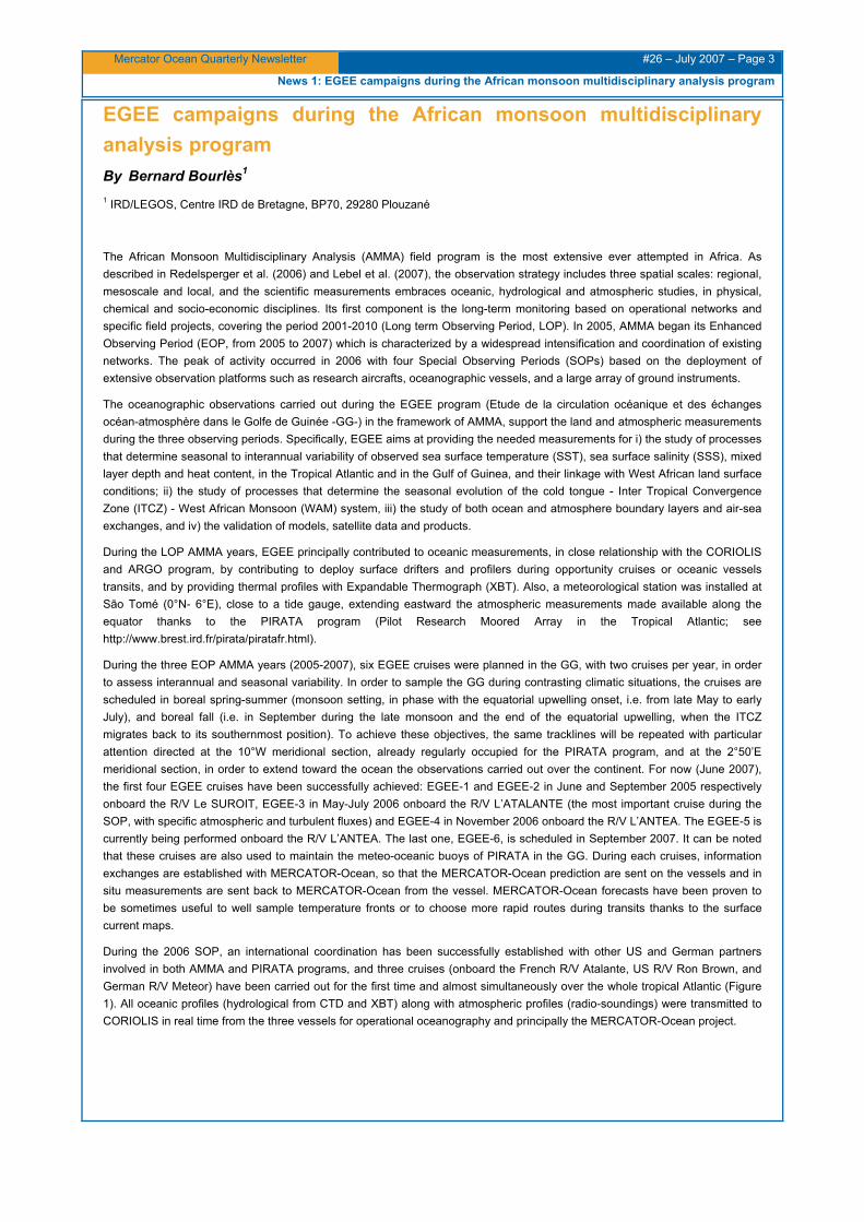
During the three EOP AMMA years (2005-2007), six EGEE cruises were planned in the GG, with two cruises per year, in order to assess interannual and seasonal variability. In order to sample the GG during contrasting climatic situations, the cruises are scheduled in boreal spring-summer (monsoon setting, in phase with the equatorial upwelling onset, i.e. from late May to early July), and boreal fall (i.e. in September during the late monsoon and the end of the equatorial upwelling, when the ITCZ migrates back to its southernmost position). To achieve these objectives, the same tracklines will be repeated with particular attention directed at the 10°W meridional section, already regularly occupied for the PIRATA program, and at the 2°50’E meridional section, in order to extend toward the ocean the observations carried out over the continent. For now (June 2007), the first four EGEE cruises have been successfully achieved: EGEE-1 and EGEE-2 in June and September 2005 respectively onboard the R/V Le SUROIT, EGEE-3 in May-July 2006 onboard the R/V L’ATALANTE (the most important cruise during the SOP, with specific atmospheric and turbulent fluxes) and EGEE-4 in November 2006 onboard the R/V L’ANTEA. The EGEE-5 is currently being performed onboard the R/V L’ANTEA. The last one, EGEE-6, is scheduled in September 2007. It can be noted that these cruises are also used to maintain the meteo-oceanic buoys of PIRATA in the GG. During each cruises, information exchanges are established with MERCATOR-Ocean, so that the MERCATOR-Ocean prediction are sent on the vessels and in situ measurements are sent back to MERCATOR-Ocean from the vessel. MERCATOR-Ocean forecasts have been proven to be sometimes useful to well sample temperature fronts or to choose more rapid routes during transits thanks to the surface current maps.
During the 2006 SOP, an international coordination has been successfully established with other US and German partners involved in both AMMA and PIRATA programs, and three cruises (onboard the French R/V Atalante, US R/V Ron Brown, and German R/V Meteor) have been carried out for the first time and almost simultaneously over the whole tropical Atlantic (Figure 1). All oceanic profiles (hydrological from CTD and XBT) along with atmospheric profiles (radio-soundings) were transmitted to CORIOLIS in real time from the three vessels for operational oceanography and principally the MERCATOR-Ocean project.

Mercator Ocean Quarterly Newsletter #26 – July 2007 – Page 4
News 1: EGEE campaigns during the African monsoon multidisciplinary analysis program
Figure 1 (from Bourlès et al., 2007)
Cruises carried out during the AMMA SOP experiment (May-July 2006), with the US Ron Brown cruise in the western and central tropical Atlantic (red line), German Meteor cruise in the central equatorial Atlantic (green line) and French Atalante cruise
in the Gulf of Guinea (blue line).
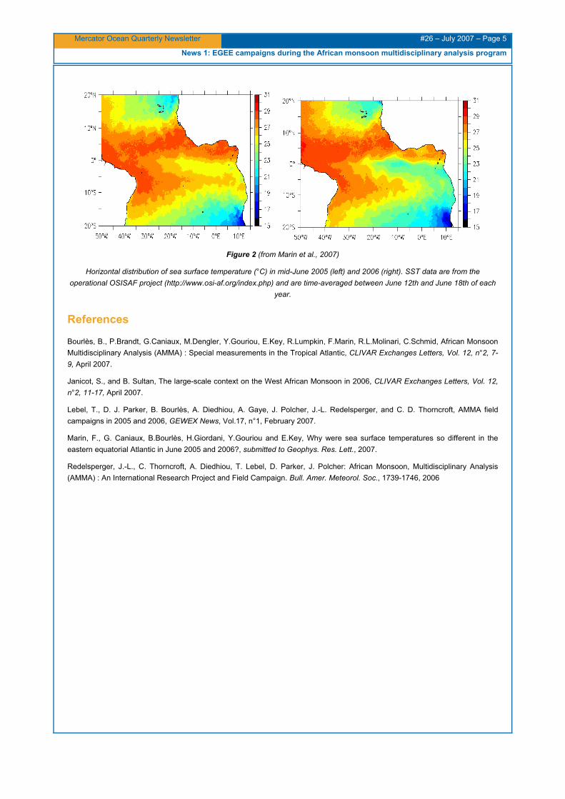
Preliminary results indicate that oceanic conditions observed during the two EGEE-1 and EGEE-3 cruises, done at one year interval in June 2005 and 2006 respectively, exhibited very different patterns: 2005 was characterized by abnormally cold sea surface temperatures -SST- in the Gulf of Guinea (cold tongue), while during 2006 the SST were particularly warm (Figure 2). It is interesting to note that 2005 (respectively 2006) was characterized by a very early (late) onset of the monsoon over the continent (around 10 July and 10 June respectively, against 20-25 June, on average). Intensive measurements of 2006 will certainly provide some insight about the reasons of this unusual behavior of the WAM (Janicot et al., 2007). Recent analysis suggests that this SST difference mainly results from a time shift in the development of the cold tongue between the two years. It is shown that a stronger than usual wind burst from the southeastern trades was responsible for the rapid and early intense cooling of the sea surface temperatures in mid-May 2005. Easterlies were also observed to be stronger in the western tropical Atlantic in April-May 2005 than in April-May 2006. Favourable preconditioned oceanic subsurface conditions were also found for this wind-burst to efficiently cool the sea surface temperature and initiate the cold tongue season (Marin et al., 2007).
Mercator Ocean Quarterly Newsletter #26 – July 2007 – Page 5
News 1: EGEE campaigns during the African monsoon multidisciplinary analysis program
Figure 2 (from Marin et al., 2007)
Horizontal distribution of sea surface temperature (°C) in mid-June 2005 (left) and 2006 (right). SST data are from the operational OSISAF project (http://www.osi-af.org/index.php) and are time-averaged between June 12th and June 18th of each
year.
References
Bourlès, B., P.Brandt, G.Caniaux, M.Dengler, Y.Gouriou, E.Key, R.Lumpkin, F.Marin, R.L.Molinari, C.Schmid, African Monsoon Multidisciplinary Analysis (AMMA) : Special measurements in the Tropical Atlantic, CLIVAR Exchanges Letters, Vol. 12, n°2, 7-9, April 2007.
Janicot, S., and B. Sultan, The large-scale context on the West African Monsoon in 2006, CLIVAR Exchanges Letters, Vol. 12, n°2, 11-17, April 2007.
Lebel, T., D. J. Parker, B. Bourlès, A. Diedhiou, A. Gaye, J. Polcher, J.-L. Redelsperger, and C. D. Thorncroft, AMMA field campaigns in 2005 and 2006, GEWEX News, Vol.17, n°1, February 2007.
Marin, F., G. Caniaux, B.Bourlès, H.Giordani, Y.Gouriou and E.Key, Why were sea surface temperatures so different in the eastern equatorial Atlantic in June 2005 and 2006?, submitted to Geophys. Res. Lett., 2007.
Redelsperger, J.-L., C. Thorncroft, A. Diedhiou, T. Lebel, D. Parker, J. Polcher: African Monsoon, Multidisciplinary Analysis (AMMA) : An International Research Project and Field Campaign. Bull. Amer. Meteorol. Soc., 1739-1746, 2006

Mercator Ocean Quarterly Newsletter #26 – July 2007 – Page 6
News 2: Tropical arrays for observing ocean and atmosphere dynamics
Tropical arrays for observing ocean and atmosphere dynamics By Fabrice Hernandez1
1 IRD/Mercator Ocean, 8/10 rue Hermès, 31520 Ramonville st Agne
During the eighties, the lack of detection of the 1982-83 El Nino event reinforced the necessity to monitor the tropical Pacific. The Tropical Atmosphere Ocean (TAO) array1 was built up from 1984 to 1994, based on 70 ATLAS (Autonomous Temperature Line Acquisition System) moorings, developed by the NOAA’s Pacific Marine Environmental Laboratory (PMEL), and deployed and maintained through a multi-national partnership of institutions in the USA, Japan, France, Taiwan, and Korea. The international Tropical Ocean Global Atmosphere (TOGA) program was mainly based on the TAO arrays. Its abundant results and outcomes demonstrated the TAO array efficiency, and allowed its sustainability for the future. In 2000, the array became TAO/TRITON (Triangle Trans-Ocean Buoy Network) with the contribution of buoys in the western Pacific (all the buoys west of 165°E) operated by the Japan Agency for Marine-Earth Science and Technology (JAMSTEC).
ATLAS is a low-cost deep ocean mooring designed to measure surface meteorological and subsurface oceanic parameters, and to transmit all data to shore in real-time via satellite relay. This way, local atmospheric fluxes can be monitored together with upper ocean dynamics. The mooring was also designed to last one year in the water before needing to be recovered for maintenance. Since the beginning, ATLAS moorings can operationally measure and transmit winds, sea surface temperature (SST), relative humidity, air temperature, and subsurface oceanic temperature at 10 depths in the upper 500 m. Some moorings along the equator were also equipped with current profilers to measure ocean velocity. After 1994, ATLAS buoys were updated by improving existing sensor accuracy, and also adding capability for measuring and transmitting in real-time salinity, rain-rate, long and shortwave radiation, barometric pressure, and ocean velocity.
The TAO/TRITON array has demonstrated its efficiency, allowing a major improvement of the tropical Pacific dynamic understanding. Its objective for the enhancement of ENSO forecasting skill, and the real time monitoring of ENSO development and impact on surrounding countries, has largely been fulfilled. It is now the Tropical Pacific observing component of the climate system (figure 1), supporting GOOS (Global Ocean Observing System) and GCOS (Global Climate Observing System).
Figure 1
Global array of all active buoys maintained by NOAA and/or with international collaborations, among which we find all the tropical TAO/TRITON and PIRATA buoys.
In the meantime, due to the TAO array success, the PIRATA (Pilot Research Moored Array in the tropical Atlantic) array has been implemented by Brazil, France and USA, in order to improve the knowledge and understanding of ocean-atmosphere variability in the tropical Atlantic. Implementation of PIRATA started in 1997 with an initial configuration of 12 ATLAS buoys (see figure 1), chosen to resolve the two main equatorial and meridional modes of climatic variability. The equatorial mode is linked with eastern equatorial Atlantic SST anomalies, analogous to ENSO in the tropical Pacific. The meridional mode is associated with SST on either side of the Inter Tropical Convergence Zone, and is linked with tropical rainfall and monsoon on surrounding 1 See http://www.pmel.noaa.gov/tao/proj_over/taohis.html for the complete historical description

Mercator Ocean Quarterly Newsletter #26 – July 2007 – Page 7
News 2: Tropical arrays for observing ocean and atmosphere dynamics
countries. PIRATA also includes three automated meteorological stations at Fernando de Noronha Island, St. Peter & St. Paul Rocks, and São Tomé Island, where a tide gauge is also operated. Two buoys location (2°S-10°W and 2°N-10°W) were abandoned during the “pilot phase” between 1997 and 2001, due to fishing vandalism. In 2006, the PIRATA array management was endorsed by the CLIVAR (Climatic Variability and Predictability) and OOPC (Ocean Observation Panel for Climate) panels, and ready for extensions.
Figure 2
PIRATA deployment plan
Three new PIRATA moorings were deployed at 8°S-30°W, 14°S-32°W and 19°S-34°W by Brazil, as part of the Southwest Extension in August 2005 (see figure 2). In order to monitor the Benguela Niños, an ATLAS buoy proposed by South Africa as the Southeast Extension, was tested at 6°S-8°E from June 2006 to June 2007. In order to capture interannual variations of the eastern ITCZ seasonal migration, as well as to monitor the evolution of upper ocean heat in the Tropical North Atlantic, and subsequently the onset of tropical cyclones, the USA proposed a PIRATA Northeast Extension (PIRATA-NE) in 2005, consisting of three ATLAS systems at 23°W, at latitudes 4°N, 11.5ºN and 20ºN and a fourth system at 20°N-38°W. This implementation began in June 2006. In addition, beginning of 2005, three PIRATA sites located in key climatic regimes in the tropical Atlantic (15°N-38°W; 0°N-23°W; and 10°S-10°W) have been heavily instrumented with additional oceanographic and meteorological instrumentation in order to provide improved estimates of mixed layer velocities, surface heat, fresh water, and momentum fluxes as well as higher vertical resolution temperature and salinity data in the mixed layer.
Both TAO/TRITON and PIRATA tropical arrays are contributing to the Ocean Sustained Interdisciplinary Timeseries Environment observation System (OceanSITES) program.
During the past ten years, efforts have been made to also start implementing a sustained tropical observing system in the Indian Ocean, which also plays a key-role in the seasonal and longer-term climate variability. In particular, the importance of i) the Indian Ocean Dipole (ENSO-like fluctuation involving coupled ocean-atmospheric interactions), as well as ii) the link and interactions at intraseasonal timescales between the Indian Ocean surface mixed layer and the highly energetic Madden-Julian Oscillation (MJO, a 30-60 day fluctuation in atmospheric winds, pressure, and rainfall that originates over the Indian Ocean), have been recognized. The MJO impacts the Asian monsoon rainfalls, the west coast USA weather, the tropical Atlantic hurricane formation, and the evolution of ENSO. Moreover, decadal warming trends in Indian Ocean sea surface temperatures have recently been shown to affect the North Atlantic Oscillation, Sahel rainfall, and other aspects of global climate.
Since 2000, several national initiatives, with in particular the Indian National Buoy Program and the Indian National Program for an Ocean Observing System (in collaboration with France), have been deploying mooring arrays in the Arabian Sea, the Bay of
• PIRATA Backbone • Brazil SW Extension • USA NE Extension • NDBC Hurricane systems • NTAS Climate Reference Station • Africa SE Extension
Mercator Ocean Quarterly Newsletter #26 – July 2007 – Page 8
News 2: Tropical arrays for observing ocean and atmosphere dynamics
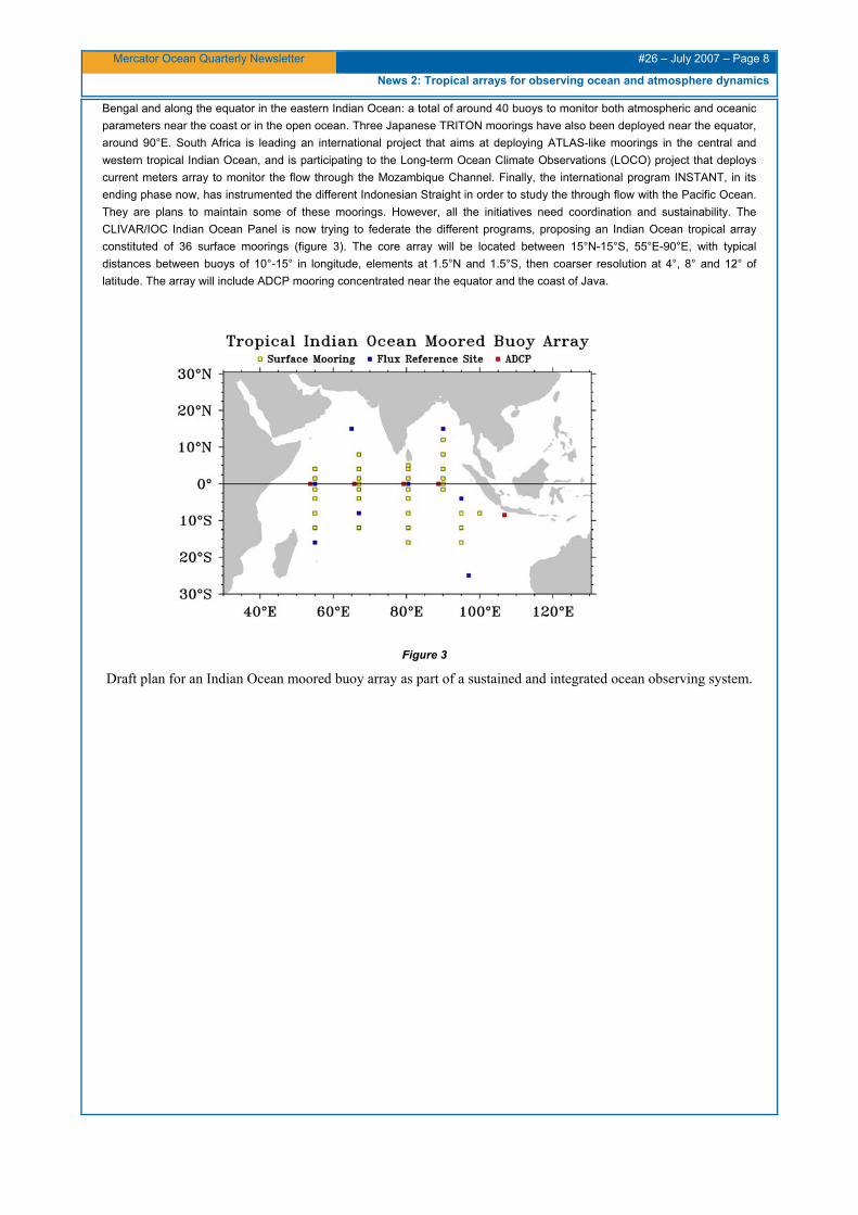
Bengal and along the equator in the eastern Indian Ocean: a total of around 40 buoys to monitor both atmospheric and oceanic parameters near the coast or in the open ocean. Three Japanese TRITON moorings have also been deployed near the equator, around 90°E. South Africa is leading an international project that aims at deploying ATLAS-like moorings in the central and western tropical Indian Ocean, and is participating to the Long-term Ocean Climate Observations (LOCO) project that deploys current meters array to monitor the flow through the Mozambique Channel. Finally, the international program INSTANT, in its ending phase now, has instrumented the different Indonesian Straight in order to study the through flow with the Pacific Ocean. They are plans to maintain some of these moorings. However, all the initiatives need coordination and sustainability. The CLIVAR/IOC Indian Ocean Panel is now trying to federate the different programs, proposing an Indian Ocean tropical array constituted of 36 surface moorings (figure 3). The core array will be located between 15°N-15°S, 55°E-90°E, with typical distances between buoys of 10°-15° in longitude, elements at 1.5°N and 1.5°S, then coarser resolution at 4°, 8° and 12° of latitude. The array will include ADCP mooring concentrated near the equator and the coast of Java.
Figure 3
Draft plan for an Indian Ocean moored buoy array as part of a sustained and integrated ocean observing system.

Mercator Ocean Quarterly Newsletter #26 – July 2007 – Page 9
The new 1/4 °Mercator Ocean global multivariate analysis and forecasting system: Tropical oceans outlook
The new 1/4° Mercator-Ocean global multivariate analysis and forecasting system: Tropical oceans outlook By: Marie Drévillon1, Laurence Crosnier3, Nicolas Ferry3, Eric Greiner2 and the PSY3V2 Team*
* The PSY3V2 Team : Mounir Benkiran2, Romain Bourdallé-Badie1, Clément Bricaud3, Edmée Durand3, Marie Drévillon1, Yann Drillet1, Nicolas Ferry3, Gilles Garric4, Eric Greiner2, Olivier Le Galloudec1, Jean-Michel Lellouche1, Fabrice Messal5, Lucas Nouël6, Laurent Parent3, Charles-Emmanuel Testut4, Benoît Tranchant1
1 CERFACS/Mercator Ocean, 8-10 rue Hermès, 31520 Ramonville St-Agne
2 CLS/Mercator Ocean, 8-10 rue Hermès, 31520 Ramonville St-Agne 3 GIP/Mercator-Océan, 8-10 rue Hermès, 31520 Ramonville St-Agne 4 MGC/Mercator-Océan, 8-10 rue Hermès, 31520 Ramonville St-Agne
5 Silogic/Mercator-Océan, 8-10 rue Hermès, 31520 Ramonville St-Agne 6 Aliasource/Mercator-Océan, 8-10 rue Hermès, 31520 Ramonville St-Agne
Introduction
This article describes the new global multivariate Mercator-Ocean analysis and forecast operational system (PSY3V2), with a special focus on Tropical Oceans. Those regions are the scene of strong large-scale ocean-atmosphere interactions, like ENSO in the Tropical Pacific. Tropical regions regularly experience extreme weather events such as for example cyclones and typhoons, which develop by exchanging energy with the warm Tropical Oceans. The latter thus need to be accurately described in order to estimate the “ocean climate”. This is the first requirement for the improvement of seasonal forecasting and climate monitoring applications. Mercator-Ocean also needs to provide accurate boundary conditions for Tropical Ocean regional models.
The PSY3V2 simulation presented here is the current Mercator-Ocean global ¼° operational system with multivariate data assimilation as well as the current MERSEA global system component (http://www.mersea.eu.org/). The simulation used in the present paper starts in April 1st 2007 until today, with a 3 months long spin up (from January 1st to March 31st 2007). A release will take place in October 2007 with mainly a better account of deep salinity and temperature measurements in the data assimilation scheme as well as a longer spin up, in order to remove remaining biases.
The PSY3V2 system has been largely improved in comparison with the previous operational system operated by Mercator-Ocean, PSY3V1. First, the ocean model of the new system includes advanced parameterisations like partial steps representation of the bottom topography, bulk formulation for the surface fluxes, a fully coupled ice model, and highly efficient advection schemes. Secondly, the data assimilation method has completely changed. Instead of assimilating only sea level anomaly (SLA henceforth) data (for PSY3V1), PSY3V2 assimilates in a multivariate way altimetric data, sea surface temperature and in situ temperature and salinity profiles. The new PSY3V2 system shows overall better skill for the analysis and forecast of the ocean state. Compared to the older version, PSY3V2 has for example almost no bias in Sea Surface Temperature (SST henceforth) and the thermocline depth variability is better represented.
First section of this article provides a short description of the new ocean model system and data assimilation scheme, and then details improvements with respect to the former monovariate system. In the second section, assimilation diagnostics are presented together with examples of model/data comparisons for various tropical regions. In the third section, we focus on the Equatorial UnderCurrent (EUC) in the Atlantic Ocean.
Description of the analysis and forecasting system
Ocean and sea ice modelling
The ¼° global forecasting system uses the NEMO (Nucleus for European Models of the Ocean) modelling code which includes the latest version of OPA 1.09 (Madec et al., 1998), coupled to the thermodynamic-dynamic sea ice model LIM2 (Louvain sea Ice Model 2) (Goose et al., 1999). The configuration has been developed in Mercator-Ocean in collaboration with the DRAKKAR working group (http://www.ifremer.fr/lpo/drakkar ).
As shown by Barnier et al. (2006), the combination of recent implementation of an energy-enstrophy conserving scheme for momentum advection with a partial steps representation of the bottom topography (Adcroft et al., 1997) yields to significant improvements in the mean circulation and in the representation of western boundary currents such as the Gulf Stream and the downstream flow of the North Atlantic Current (not shown). Moreover, the model ¼° horizontal solution is often comparable to ones obtained with 1/6°or 1/10° resolution on aspects concerning mean flow patterns and distribution of eddy kinetic energy (not

Mercator Ocean Quarterly Newsletter #26 – July 2007 – Page 10
The new 1/4 °Mercator Ocean global multivariate analysis and forecasting system: Tropical oceans outlook
shown). In order to better resolve the upper layers, the vertical grid has been refined especially at the surface, with now 50 verticals levels (against 46 before), leading to layer thickness ranging from 1 to 20 meters at the surface and 500 meters for the deep layers. With this surface refined mesh, the vertical grid is now designed to improve the circulation in the coastal shelves and represent more accurately the impact of the atmospheric diurnal cycle which will be explicitly modelled in the future.
The atmospheric forcing fields driving the system are calculated using the empirical bulk parameterisation described by Goosse et al. (2001). A systematic bias in the precipitations is removed thanks to GPCP precipitation observations (Huffman et al. 1997) when available. The bias is removed thanks to a predictor computed from these observations.
The sea ice is fully prognostic with the implementation of the LIM2 model (Goose et al., 1999). With sea ice concentration, sea ice and snow thickness, sea ice drift and sea ice thermal content prognosed by this multi-layer model based on the Semtner (1976) 3-layers and the Hibler (1979) visco-plastic formulations, analysis and forecasts will handle most of the sea ice cycle processes.
Data assimilation
The data assimilation method relies on a reduced order Kalman filter using a 3D modal decomposition of the ocean forecast error covariance and based on the SEEK formulation introduced by Pham et al. (1998) in the context of mesoscale ocean models. The forecast error covariance is time dependant and is based on the statistics of a collection of 3D ocean state anomalies (between 150 and 300). The control variables are the 3D temperature, salinity fields and the barotropic height. The formulation used at Mercator-Ocean also includes an adaptive scheme for the model error variance.
The assimilated data consist of satellite SLA and SST data, as well as in situ temperature (T) and salinity (S) profiles. Along track altimetry is provided by the SSALTO/DUACS data centre (gathering all available missions: JASON, ENVISAT and GFO). SST at 0.5°x0.5° spatial resolution comes from NCEP (RTG_SST product, Thiébaux et al. 2003) and CORIOLIS centre (Ifremer) delivers in situ T and S profiles. It is worth noting that the model SLA is calculated using the Rio et al. (2005) version 5.1 mean dynamic topography (MDT). The associated observation error includes the satellite instrumental error plus spatially variable MDT and model representation errors. For each kind of data set, innovations (observation minus model) are computed at the observation geographical location and at appropriate time (First Guess at Appropriate Time, FGAT).
The data assimilation produces after each analysis global ocean temperature, salinity and barotropic height increments. Physical balance operators allow deducing from these increments zonal and meridional velocity fields as well as sea surface height increments. It is planned in a near future to augment the size of the control vector by including the 2 horizontal components of the velocity in order to produce statistically velocity increments.
The length of the assimilation cycle is 7 days and on each Wednesday (day D), PSY3V2 performs a two week hindcast plus a 2 week forecast. The first analysis (day D-7) performed in ‘reanalysis’ mode is called the best estimate analysis whereas the second one (day D) is called the ‘nowcast’.
Performances of the system in the Tropical Oceans
Comparisons with in situ measurements in the upper layers
In the tropical oceans, in situ data which are assimilated in the system include, in addition to the ARGO floats and cruises measurements, in situ measurement provided by the TAO (for the Pacific) and PIRATA (for the Atlantic) arrays of moorings. A TAO array is also being implemented in the Tropical Indian Ocean (http://www.pmel.noaa.gov/tao/jsdisplay/) (see Hernandez, this issue).
The aim in this section is to compare the PSY3V2 system to available in situ observations in the tropics using forecast outputs which have not yet undergone any data assimilation of observation for the current assimilation cycle. Observations can thus in this case be considered as independent, as they are not assimilated yet in the system when the model-observations misfit is calculated. This misfit (which is the opposite of what is called the model innovation) is calculated for each observation during each 7-day assimilation cycle.
In the three following sections, we use Tropical Oceans boxes (figure 1) inherited from the ENACT European project (ENACT, ENhAnced ocean data assimilation and ClimaTe prediction, 2005), to display an overview of the PSY3V2 upper layers performances in the Pacific, Indian and Atlantic tropical oceans respectively.

Mercator Ocean Quarterly Newsletter #26 – July 2007 – Page 11
The new 1/4 °Mercator Ocean global multivariate analysis and forecasting system: Tropical oceans outlook
Figure 1
oceanic regions for data assimilation diagnostics defined in the framework of the ENACT project. In this study, we focus on the red boxes (Tropical Oceans)
Pacific Ocean
In the Nino3 and Nino4 Pacific Ocean boxes (Figures 2 and 3 respectively), on average, PSY3V2 forecasts stay close to the in situ observations. The temperature bias is less than 0.5 °C, and the salinity bias does not exceed locally 0.05 psu, which is small in comparison with the PSY3V1 system (not shown). The signature of the thermocline can be seen through all the standard deviation diagnostics, as maximum errors occur where the vertical gradient of temperature is strong. Nevertheless, the location of the thermocline is more realistic in PSY3V2 than in PSY3V1 (not shown).
The SST bias is drastically reduced in PSY3V2 compared to PSY3V1, especially in Nino4 (Figure 4). This improvement is mainly due to the bulk formulae forcing fields used, as well as to the model parameterisations in the tropics applied, together with the multivariate RTG-SST (Thiébaux et al., 2003) data assimilation.

Mercator Ocean Quarterly Newsletter #26 – July 2007 – Page 12
The new 1/4 °Mercator Ocean global multivariate analysis and forecasting system: Tropical oceans outlook
Figure 2
For the box number 13 “Nino3” from figure 1 from top to bottom, time series of the number of in situ observations in the first 700 m, of the mean difference between the PSY3V2 forecast and the in situ observations, and of the standard deviation of
difference between the forecast and the observations. The forecast data are interpolated at the geographical location of the observations, on the left panel for temperature (°C), and on the right panel for salinity (psu).
Figure 3
same as Figure 2 but for the box number 14 « Nino4 » from Figure 1

Mercator Ocean Quarterly Newsletter #26 – July 2007 – Page 13
The new 1/4 °Mercator Ocean global multivariate analysis and forecasting system: Tropical oceans outlook
Figure 4
global 1/4° PSY3V1 and PSY3V2 systems averaged SST (°C) in the Niño 3 and 4 boxes, compared with observed products : Reynolds et al. (2002) and SAFO ( Roquet, 2006), CMS Lannion).
Indian Ocean
In the Ind1 (Figure 5) and Ind2 (not shown) Indian boxes, the PSY3V2 system behaves in a similar way. A salinity bias towards fresher waters appears under 500 m in the Ind1 box (Figure 5), but does not increase with time. The present PSY3V2 system does not take into account enough deep salinity and temperature measurements. This bias should be weaker in the next version of the system (October 2007 release), which will benefit from a longer spin up and where deep salinity and temperature measurements will be better taken into account.
Figure 5
same as Figure 2 but for the box number 19 “Ind1” from Figure 1
NINO 3
Temperature in Nino boxes SST (Reynolds OI-v2 weekly) SST (PSY3V1) SST (PSY3V2) SST SAFO
NINO 4
Mercator Ocean Quarterly Newsletter #26 – July 2007 – Page 14
The new 1/4 °Mercator Ocean global multivariate analysis and forecasting system: Tropical oceans outlook
Atlantic Ocean
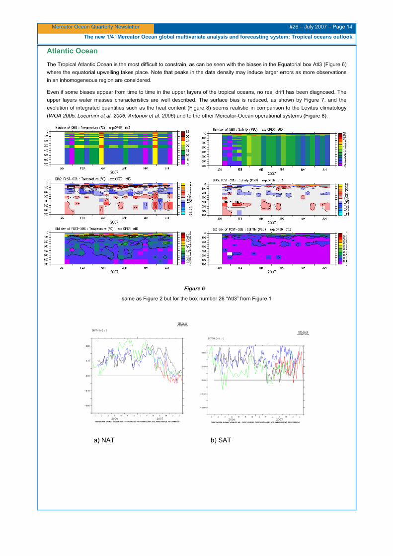
The Tropical Atlantic Ocean is the most difficult to constrain, as can be seen with the biases in the Equatorial box Atl3 (Figure 6) where the equatorial upwelling takes place. Note that peaks in the data density may induce larger errors as more observations in an inhomogeneous region are considered.
Even if some biases appear from time to time in the upper layers of the tropical oceans, no real drift has been diagnosed. The upper layers water masses characteristics are well described. The surface bias is reduced, as shown by Figure 7, and the evolution of integrated quantities such as the heat content (Figure 8) seems realistic in comparison to the Levitus climatology (WOA 2005, Locarnini et al. 2006; Antonov et al. 2006) and to the other Mercator-Ocean operational systems (Figure 8).
Figure 6
same as Figure 2 but for the box number 26 “Atl3” from Figure 1
a) NAT b) SAT

Mercator Ocean Quarterly Newsletter #26 – July 2007 – Page 15
The new 1/4 °Mercator Ocean global multivariate analysis and forecasting system: Tropical oceans outlook
c) TASI d) TNA
e) TSA f)
Figure 7
Time series of the Sea Surface Temperature Anomalies (ºC) relative to the Reynolds 1971-2000 climatology (Reynolds et al. 2002), in various Atlantic boxes (panel (f)) in 3 Mercator-Ocean operational systems: the Global 1/4º monovariate PSY3V1
(black line), the Global 1/4º multivariate PSY3V2 (red line) and the Atlantic 1/3º multivariate PSY1V2 (blue line), as well as the Reynolds et al. (2002) analysis (green line) from July 2006 until July 2007, in the boxes (a) NAT, (b) SAT, (c) TASI, (d) TNA, (e)
TSA. Panel (f) shows the location of each box.
Figure 8
Heat Content (Joules) in the Gulf of Guinea (4ºS-7ºN, 15ºW-15ºE) in 3 Mercator-Ocean operational systems: the Global 1/4º monovariate PSY3V1 (black line) , the Global 1/4º multivariate PSY3V2 (red line) and The Atlantic 1/3º multivariate PSY1V2 (green line), and the Levitus (WOA 2005) climatology (blue line), from September 2006 until July 2007, (left) in the top 300
meters, (right) above the 20 ºC isotherm
Mercator Ocean Quarterly Newsletter #26 – July 2007 – Page 16
The new 1/4 °Mercator Ocean global multivariate analysis and forecasting system: Tropical oceans outlook
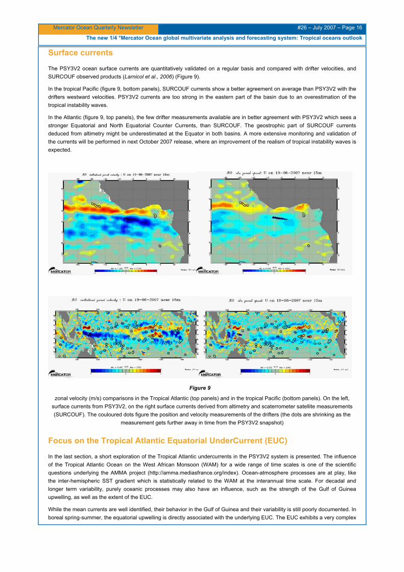
Surface currents
The PSY3V2 ocean surface currents are quantitatively validated on a regular basis and compared with drifter velocities, and SURCOUF observed products (Larnicol et al., 2006) (Figure 9).
In the tropical Pacific (figure 9, bottom panels), SURCOUF currents show a better agreement on average than PSY3V2 with the drifters westward velocities. PSY3V2 currents are too strong in the eastern part of the basin due to an overestimation of the tropical instability waves.
In the Atlantic (figure 9, top panels), the few drifter measurements available are in better agreement with PSY3V2 which sees a stronger Equatorial and North Equatorial Counter Currents, than SURCOUF. The geostrophic part of SURCOUF currents deduced from altimetry might be underestimated at the Equator in both basins. A more extensive monitoring and validation of the currents will be performed in next October 2007 release, where an improvement of the realism of tropical instability waves is expected.
Figure 9
zonal velocity (m/s) comparisons in the Tropical Atlantic (top panels) and in the tropical Pacific (bottom panels). On the left, surface currents from PSY3V2, on the right surface currents derived from altimetry and scaterrometer satellite measurements (SURCOUF). The couloured dots figure the position and velocity measurements of the drifters (the dots are shrinking as the
measurement gets further away in time from the PSY3V2 snapshot)
Focus on the Tropical Atlantic Equatorial UnderCurrent (EUC)
In the last section, a short exploration of the Tropical Atlantic undercurrents in the PSY3V2 system is presented. The influence of the Tropical Atlantic Ocean on the West African Monsoon (WAM) for a wide range of time scales is one of the scientific questions underlying the AMMA project (http://amma.mediasfrance.org/index). Ocean-atmosphere processes are at play, like the inter-hemispheric SST gradient which is statistically related to the WAM at the interannual time scale. For decadal and longer term variability, purely oceanic processes may also have an influence, such as the strength of the Gulf of Guinea upwelling, as well as the extent of the EUC.
While the mean currents are well identified, their behavior in the Gulf of Guinea and their variability is still poorly documented. In boreal spring-summer, the equatorial upwelling is directly associated with the underlying EUC. The EUC exhibits a very complex

Mercator Ocean Quarterly Newsletter #26 – July 2007 – Page 17
The new 1/4 °Mercator Ocean global multivariate analysis and forecasting system: Tropical oceans outlook
dynamic and its eastern termination is still not understood. For example the two recent EQUALANT cruises, carried out in boreal summer 1999 and 2000, have shown a strong one year-interval variability of the EUC at 10°W, and revealed its disappearance east of 0°E (Bourles et al, 2002) along with important differences in SST at 10°W.
Figure 10 shows that the EUC seasonal variability is well captured by PSY3V2, as it intensifies at 5°W from March to May, which is the classical period of the onset of the WAM. The EUC does not extend further east than 6°E in the system, except maybe in May, with a week intensification of the Eastward current at 50m depth. The current PSY3V2 operational system and its future reanalysis over the period (1950-2007) will allow in the near future studying the influence of the Tropical Atlantic Ocean on the WAM for a wide range of time scales.
10°W 5°W 6°E
March 2007
April 2007
May 2007
Figure 10
Latitude sections of zonal velocitity (m/s) in the first 300m at 10°W (left panels) at 5°W (middle panels) and at 6°E (right panels) on monthly average for March 2007 (upper panels), April 2007 (middle panels) and May 2007 (lower panels)
Conclusion
The PSY3V2 results in the Tropical Oceans are encouraging: PSY3V2 appears to be a powerful tool for monitoring the ocean climate. Its performances in the Tropical Oceans equal that of PSY1V2 in the Tropical Atlantic. The model parameterisations and vertical resolution even improve the accuracy of the thermocline location, and of the circulation. These qualities make it eligible to perform a global reanalysis, which will be done in collaboration with the research community, starting in 2008. The PSY3V2 reanalysis system will improve in the near future, with the addition of the Incremental Analysis Update (IAU) scheme,
Mercator Ocean Quarterly Newsletter #26 – July 2007 – Page 18
The new 1/4 °Mercator Ocean global multivariate analysis and forecasting system: Tropical oceans outlook
which limits the data assimilation shocks and allows a better physical and temporal consistency of the ocean variables. The next step in the MERSEA framework involves the development of the global eddy resolving (1/12°) system. A North Atlantic version at 1/12° is already in progress with interannual free experiments already performed.
References
Adcroft A., C Hill, and J Marshall, 'Representation of topography by shaved cells in a height coordinate ocean model', Mon. Weather Rev., 125, 2293-2315.2(1997).
Antonov, J. I., R. A. Locarnini, T. P. Boyer, A. V. Mishonov, and H. E. Garcia, 2006. World Ocean Atlas 2005, Volume 2: Salinity. S. Levitus, Ed. NOAA Atlas NESDIS 62, U.S. Government Printing Office, Washington, D.C., 182 pp.
Barnier B., G Madec, T. Penduff, J.M. Molines, A.M. Treguier, J. Le Sommer, A. Beckmann, A. Biastoch, C. Boning, J. Dengg, C. Derval, E. Durand, S. Gulev, E. Remy, C. Talandier, S. Theetten, M. Maltrud, J. McLean, B. De Cuevas, 'Impact of partial steps and momentum advection schemes in as global ocean circulation model at eddy permitting resolution', Ocean Dynamics, DOI 10.1007/s10236-006-0082-1(2006).
Bourlès B., M. D’Orgeville, G. Eldin, Y. Gouriou, R. Chuchla, Y. DuPenhoat and S. Arnault, On the evolution of the thermocline and subthermocline currents in the Equatorial Atlantic. Geophysical Research Letters 29 (16). doi 10.1029/2002/GL015098 (2002)
ENACT, Enhanced Ocean Data Assimilation and Climate Prediction A European Commission Framework 5 project: contract number EVK2-CT2001-00117, 1 January 2002 to 31 December 2004, Final Report: public: version 1, http://www.lodyc.jussieu.fr/ENACT/index.html, 28 February 2005.
Goosse H. and T Fichefet, 'Importance of ice-ocean interactions for the global ocean circulation: a model study, J. Geophys. Res., 104, 23,337-23,355, (1999).
Goosse H., J-M Campin, E Deleersnijder, T Fichefet, P-P Mathieu, MAM Maqueda, and B Tartinville, Description of the CLIO model version 3.0, Institut d'Astronomie et de Geophysique Georges Lemaitre, Catholic University of Louvain (Belgium) , (2001).
Hibler W.D.I., 'A dynamic thermodynamic sea ice model', J. Phys. Oceanogr., 9, 815-846, (1979).
Huffman G.J. and P.A. Arkin and A. Chang and R. Ferraro and A. Gruber and J. E. Janowiak and R.J. Joyce and A. McNab and B. Rudolf and U. Schneider and P. Xie : The Global Precipitation Climatology Project (GPCP) Combined Precipitation Data Set, Bull. Amer. Met. Soc., Vol78, pp5-20 (1997).
Larnicol, G., Guinehut, S., Rio, M.-H., Drévillon, M., Faugere, Y., Nicolas, G., 2006: The Global Observed Ocean Products of the French Mercator Project. Proceddings of the symposium: "15 years of Progress in Radar Altimetry", Venice, March 2006.
Locarnini, R. A., A. V. Mishonov, J. I. Antonov, T. P. Boyer, and H. E. Garcia, 2006. World Ocean Atlas 2005, Volume 1: Temperature. S. Levitus, Ed. NOAA Atlas NESDIS 61, U.S. Government Printing Office, Washington, D.C., 182 pp.
Madec G., P Delecluse, M Imbard, and C Levy, OPA 8.1 general circulation model reference manual, Notes de l'Institut Pierre-Simon Laplace (IPSL) - Université P. et M. Curie, B102 T15-E5, 4 place Jussieu, Paris cédex 5, 91p, (1998).
Pham D. T., J. Verron, and M C Roubaud, 'A singular evolutive extended Kalman filter for data assimilation in oceanography', Journal of Marine Systems, 16, 323-340, (1998).
Reynolds, R.W., N.A. Rayner, T.M. Smith, D.C. Stokes, and W. Wang, 2002: An Improved In Situ and Satellite SST Analysis for Climate. J. Climate, 15, 1609-1625.
Rio, M.-H., Schaeffer, P., Hernandez, F., Lemoine, J.-M. , 2005. The estimation of the ocean Mean Dynamic Topography through the combination of altimetric data, in-situ measurements and GRACE geoid: From global to regional studies. Proceedings of the GOCINA Workshop in Luxembourg (April, 13-15 2005)
Roquet H., 2006, Mersea satellite activities and products, Mercator-Ocean newsletter n°22, July 2006, http://www.mercator-ocean.fr/documents/lettre/lettre_22_en.pdf
Semtner A. J., 'A model for the thermodynamic growth of sea ice in numerical investigations of climate', J. Phys. Oceanogr., 6, 379-389, (1976).
Thiébaux J. , E Rogers, W Wang, and B Katz, 'A new high resolution blended real time global sea surface temperature analysis', Bulletin of the American Meteorological Society, 84, 645-656, (2003). see also http://polar.ncep.noaa.gov/sst/oper/Welcome.html
Mercator Ocean Quarterly Newsletter #26 – July 2007 – Page 19
“Bulletin climatique global” of Météo-France: a contribution of Mercator-Ocean
“Bulletin Climatique Global” of Météo-France: a contribution of Mercator-Ocean to the seasonal prediction of El Niño 2006-07 By: Silvana Ramos Buarque1, Christophe Cassou2, Isabelle Charon3 and Jean-François Gueremy4 1 GIP/Mercator Ocean, 8/10 rue Hermès, 31520 Ramonville st Agne 2 CERFACS, 42 avenue Gaspard Coriolis, 31057 Toulouse cedex 01 3 Météo France (DClim), 42 avenue Gaspard Coriolis, 31057 Toulouse cedex 01 4 CNRM ,42 avenue Gaspard Coriolis, 31057 Toulouse cedex 01
Introduction
Since 2005, the “Centre National de Recherches Météorologiques” (CNRM) has developed and maintained a seasonal forecast (SF) system based on the ARPEGE-Climat-OPA coupled ocean-atmosphere model (Piedelievre, 2002). The monthly oceanic initial states are provided by the “Groupement d’Intéret Public” Mercator-Océan (Ferry et al., 2007). The atmospheric initial states come from the ECMWF analyses and a 40-member ensemble of 7 months long is carried out on a monthly basis. In this framework, the “Direction de la Climatologie” of Météo-France has implemented a multi-disciplinary group including experts from CERFACS and Mercator-Océan to analyze the results of real-time SF systems. The aim of this group is to publish a monthly “Bulletin Climatique Global” (BCG) based on the interpretation of the previous months observations and the analyses of several SF systems. The editorial board is divided into groups of expertise and the outcome of their discussion leads to a consensual prediction.
More specifically, since February 2006, this group meets on a monthly basis in order to:
• analyze the state of the climatic system in progress (main modes of variability like El Niño Southern Oscillation (ENSO), North Atlantic Oscillation (NAO) etc.) ;
• produce seasonal forecasts for temperature and precipitation in particular for France including French Overseas Regions: Antilles, New Caledonia, French Polynesia, French Guiana, “La Réunion”, Mayotte, “Wallis et Futuna” and “Saint-Pierre et Miquelon”;
• improve the general understanding of the coupled system.
The contribution of Mercator-Océan consists in exploiting real-time systems of oceanic medium-range forecasts developed at Mercator-Océan such as the Global monovariate 1/4° forecast systems (PSY3V1), in order to understand the past season ocean variability. The availability of a reference constrains the choice of the system used. Mercator-Océan also assess and evaluate the provided initial oceanic states for SF and the analyzed oceanic state from the best system available.
Seasonal Forecasts are disseminated from http://www.meteofrance.com .
Initial Oceanic states used for seasonal forecast Initial states used in the SF system come from the “Océan PArallélisé” (OPA) primitive equation model used in the so-called ORCA2 configuration. The horizontal mesh is orthogonal and curvilinear on the sphere and has a 2o-degree horizontal resolution on average. The grid has two poles in northern hemisphere used to overcome the North Pole singularity (Madec and Imbard, 1996). The resolution is refined in latitude near the equator to better resolve the equatorial dynamics. A rigid lid is assumed at the sea surface.
For the ORCA2 reference model, surface heat and momentum fluxes are provided by the ERA-40 reanalysis. For the real-time forecast, ECMWF analyses are used to force the ocean model. A feedback term is added to the specified heat flux (Barnier, 1998):
)(0 SSTSSTdTdQQQ OBSMOD−+=
where Q0 is the heat flux prescribed from the re-analysis, SSTOBS is the daily Real Time Global Sea Surface Temperature
(Thiébaux et al., 2003), SSTMOD is the model SST and dTdQ/ is a negative feedback coefficient equal to 12200 −−− KWm .
Mercator Ocean Quarterly Newsletter #26 – July 2007 – Page 20
“Bulletin climatique global” of Météo-France: a contribution of Mercator-Ocean
The difference between SSTMOD and SSTOBS times dQ/dT is called the relaxation term and is very strong in our case. The
intent is to perform simple SST data assimilation by the way of a nudging technique.
The analyzed and forecast oceanic state
The ORCA2 system described above is used for the SF initial oceanic state. In order monitor El Niño event in the framework of the “Bulletin Climatique Global”, it is rather the best available real-time forecast Mercator-Ocean system (i.e the monovariate global 1/4° forecast system, PSY3V1) which is used. The ORCA2 system is also used here to assess the El Nino event, as a complement.
The MERCATOR systems have been regularly upgraded by improving the assimilation schemes and/or by expanding the geographical coverage from regional to global ocean. In the tropical Pacific, El Niño event is first monitored using the monovariate global 1/4° forecast system (PSY3V1). This system operates with 0.25 degrees of horizontal resolution and 46 vertical levels assimilating satellite data of Sea Level Anomalies SSALTO/DUACS. Currently, the multivariate global 1/4° forecast system PSY3V2 assimilating both in-situ data and SSTs in addition to altimetry, is replacing PSY3V1 (Drevillon et al., 2006).
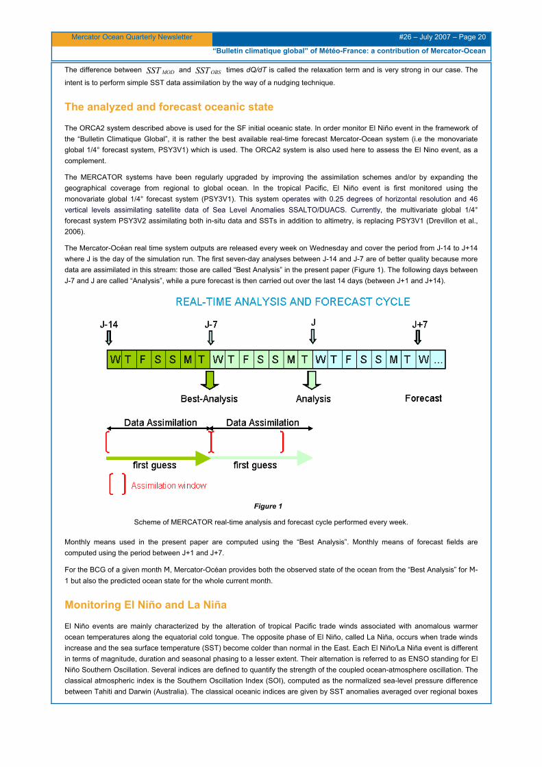
The Mercator-Océan real time system outputs are released every week on Wednesday and cover the period from J-14 to J+14 where J is the day of the simulation run. The first seven-day analyses between J-14 and J-7 are of better quality because more data are assimilated in this stream: those are called “Best Analysis” in the present paper (Figure 1). The following days between J-7 and J are called “Analysis”, while a pure forecast is then carried out over the last 14 days (between J+1 and J+14).
Figure 1
Scheme of MERCATOR real-time analysis and forecast cycle performed every week.
Monthly means used in the present paper are computed using the “Best Analysis”. Monthly means of forecast fields are computed using the period between J+1 and J+7.
For the BCG of a given month M, Mercator-Océan provides both the observed state of the ocean from the “Best Analysis” for M-1 but also the predicted ocean state for the whole current month.
Monitoring El Niño and La Niña
El Niño events are mainly characterized by the alteration of tropical Pacific trade winds associated with anomalous warmer ocean temperatures along the equatorial cold tongue. The opposite phase of El Niño, called La Niña, occurs when trade winds increase and the sea surface temperature (SST) become colder than normal in the East. Each El Niño/La Niña event is different in terms of magnitude, duration and seasonal phasing to a lesser extent. Their alternation is referred to as ENSO standing for El Niño Southern Oscillation. Several indices are defined to quantify the strength of the coupled ocean-atmosphere oscillation. The classical atmospheric index is the Southern Oscillation Index (SOI), computed as the normalized sea-level pressure difference between Tahiti and Darwin (Australia). The classical oceanic indices are given by SST anomalies averaged over regional boxes
Mercator Ocean Quarterly Newsletter #26 – July 2007 – Page 21
“Bulletin climatique global” of Météo-France: a contribution of Mercator-Ocean
named NINO 1-2, 3, 3-4 and 4 and 3-4 respectively from the South American coast to the central equatorial Pacific (Trenberth and Stepaniak, 2001). Other indices are estimated from anomalous 850 mb zonal wind to describe the low-level atmospheric circulation. Outgoing longwave radiation estimated from satellites is also used as a proxy for deep convection.
The Climate Prediction Center (CPC) (http://www.cpc.noaa.gov/products ) gives a complete analysis of ENSO events. Those are currently based on in-situ ocean data such as the TAO buoy network (http://www.pmel.noaa.gov/tao/jsdisplay/), and satellites observations (http://www.jason.oceanobs.com/html/), both providing a real-time monitoring.
El Niño predictions have been improving over the last 15 years along with the improvement of global coupled ocean-atmosphere models or thanks to the assimilation of SST analysis and oceanic fields in forced oceanic models used to get initial ocean conditions for SF.
Within this framework, a bulletin for ENSO forecast is prepared on a monthly basis through a collaborative effort between the World Meteorological Organization (in which the SF system from Météo-France is included) and the International Research Institute for Climate and Society (IRI) as a contribution to the United Nations Inter-Agency Task Force on Natural Disaster Reduction (http://www.wmo.ch/pages/prog/wcp/wcasp/enso_updates.html). A summary of current ENSO forecasts is also provided on http://www.pmel.noaa.gov/tao/elnino/forecasts.html. Various kinds of forecast schemes are included from simple statistical models to more complete dynamical coupled models.
The overview in the paragraph above shows why it is very important to evaluate the ability of the Mercator-Océan systems to observe and predict ENSO events. This study shows how it is possible to observe, analyse and better understand ENSO variability with Mercator global ocean analyses. The kind of study presented here allows the BCG team to better understand the couped SF performed with Mercator oceanic initial conditions.
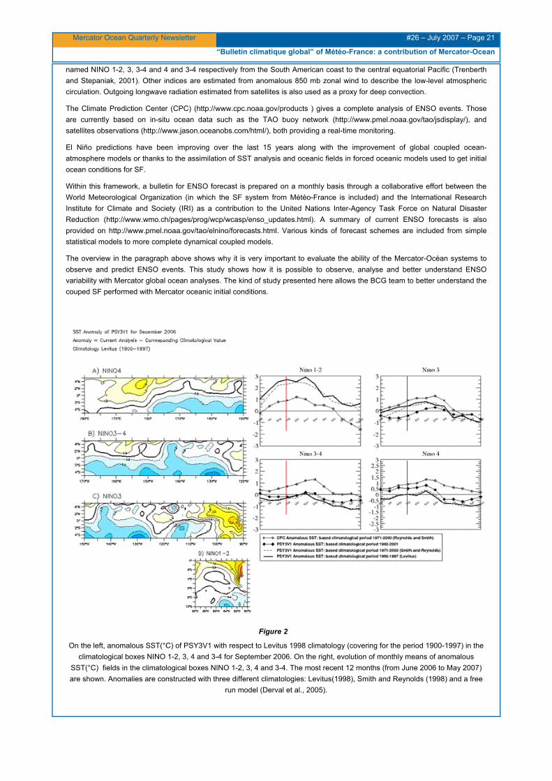
Figure 2
On the left, anomalous SST(°C) of PSY3V1 with respect to Levitus 1998 climatology (covering for the period 1900-1997) in the climatological boxes NINO 1-2, 3, 4 and 3-4 for September 2006. On the right, evolution of monthly means of anomalous
SST(°C) fields in the climatological boxes NINO 1-2, 3, 4 and 3-4. The most recent 12 months (from June 2006 to May 2007) are shown. Anomalies are constructed with three different climatologies: Levitus(1998), Smith and Reynolds (1998) and a free
run model (Derval et al., 2005).

Mercator Ocean Quarterly Newsletter #26 – July 2007 – Page 22
“Bulletin climatique global” of Météo-France: a contribution of Mercator-Ocean
The performance of the global monovariate PSY3V1 real-time system in simulating the observed 2006-2007 El Niño is given in Figure 2. Predicted SST anomalies are computed over the NINO12, NINO3, NINO4 and NINO34 boxes using three different climatological references: Levitus (1998), Smith and Reynolds (1998) and the free model simulation over the period 1992-2001 (Derval et al., 2005).
Left panels of Figure 2 show that in September 2006, anomalous SST compared to Levitus climatology are already positive in NINO12. Right panels of Figure 2 show the evolution of the anomalous SST simulated by PSY3V1 and compared to Climate Prediction Center (CPC) estimates. In the NINO12 box, PSY3V1 anomalous SST with respect to Levitus as well as Smith and Reynolds climatologies are much larger than CPC. The anomalies in the NINO 3, 3-4 and 4 are smaller than observed for the CPC and sometimes with an opposite signal.
The features of the anomalies tendencies are qualitatively comparable. The anomalies in respect to Smith and Reynolds climatology covers the same period beginning in 1971 and ending in 2000. The anomalies in respect to Levitus climatology covers the period 1900-1997. Note that the differences between the CPC and PSY3V1 anomalies related to Smith and Reynolds climatological basis are similar to the ones observed for the Levitus climatological basis. This shows that in this regions the period of the climatology does not explains the differences.
The PSY3V1 anomalies related to a free run of the same model used in PSY3V1 over the period 1992-2001 is also shown (solid line with rhombus). This free run is independent from the system assimilating only sea level anomalies satellite data. Thus, the difference between the CPC and PSY3V1 anomalies are mainly due to a model bias which is not corrected by the data assimilation (this version of the system does not include any SST data assimilation).
Observed El Niño 2006-07
Figure 3 shows the global SST anomalies for ORCA2 in January 2007 used as initial conditions for SF. January corresponds to the peak of the 2006-2007 event as also described in Figure 2. Tropical Pacific conditions are warmer than averaged by about 1.5°C in the NINO3 region. Premises of a rapid termination of the event are visible in the central Pacific with cold anomalies along the equator located slightly to the east of the dateline.
Figure 3
Sea Surface Temperature (SST) anomalies for January 2007 from ORCA2 compared to the model reference for the period 1989-93.

Mercator Ocean Quarterly Newsletter #26 – July 2007 – Page 23
“Bulletin climatique global” of Météo-France: a contribution of Mercator-Ocean
Table 1 summarizes the monthly statements written in the BCG regarding the anomalous oceanic subsurface conditions along the equator in the Pacific. The depth of thermocline is approximated by the depth of the 20 degrees isotherm (D20). Figure 4 gives the Hovmöller diagram of the D20 anomaly from Nov 2006 to Jan 2007 showing the full development of the 2006-2007 El Niño event. All steps described on Table 1 can be also followed on Figure 4. Vertical sections of temperature in the tropical Pacific are shown on the right part of the Table 1.
Date of Production
Seasonal Forecast Period
Seasonal Forecast
Best Analysis (PSY3V1)
Nov 2006
DJF
Positive temperature anomalies observed beneath the surface in the middle-west of the basin are strengthening; the situation is consistent with the development of an El Niño event. The oceanic thermocline (20°C isotherm depth on Figure 4) along the equator is thus deeper than normal. At the surface, oceanic structures are consistent with the development of a warm event for the end of the year off the coast of Peru assuming the propagation of the warm reservoir following a Kelvin wave paradigm
October
Dec 2006 JFM
In the Tropical Pacific, warm water started propagating eastward while rapidly strengthening: a positive anomaly of the 20°C isotherm depth is observed on the center of the basin (Figure 4). On the West part of the Tropical Pacific basin, beneath the surface, negative anomalies appear and could be a premise of the rapid termination of the warm event.
November
Jan 2007 FMA
The core of positive anomalies observed last month in the center of the basin weakened and moved rapidly eastwards corresponding to the mature phase of ENSO. In the west of the basin, a cold anomaly is observed beneath the surface between 100 and 200m depth. These conditions are favorable to the end of the episode still based on their eastward propagation based on Kelvin waves.
December
Table 1
Main paragraphs from the BCG concerning ocean analysis for the El Niño forecast.
Analyzed sections of temperature for S-O-N-D months show that subsurface positive anomalies intensify along the period and propagate eastwards. Their dissipation starts in January as shown in Figure 5, especially in the center of the basin. The further evolution of the D20 shows the displacement of a cold Kelvin wave from February onward while positive anomalies appear on the west part of the basin. The latter situation is consistent with the end of the 2006-2007 El Niño event and the development of neutral to colder conditions.

Mercator Ocean Quarterly Newsletter #26 – July 2007 – Page 24
“Bulletin climatique global” of Météo-France: a contribution of Mercator-Ocean
Figure 4
Hovmoller diagram of the D20 (depth of the 20°C isotherm) anomaly in meters. Notes the propagation of the positive anomalies eastwards from October to January.
Figure 5 shows the anomalous SST for ORCA2 in the tropical Pacific from March to May 2007. The reference run covers the period 1989-1993 (Ramos Buarque et al., 2003). The patterns clearly display the end of the 2006-2007 El Niño event. From March to May, a cold anomaly starts at the west coast of South America and stretches thousands of kilometers along the equator. This announces the change from the Niño state to a neutral state: the SF for AMJ advertise the probability of a La Niña event for the summer 2007.

Mercator Ocean Quarterly Newsletter #26 – July 2007 – Page 25
“Bulletin climatique global” of Météo-France: a contribution of Mercator-Ocean
Figure 5
Anomalous SST for ORCA2 in the boxes NINO12, 3, 34 and 4 from March to May 2007 respectively from the top to bottom. The reference is a free run for the period 1989-1993 (Ramos Buarque et al., 2003).
Conclusions
Within the seasonal forecast framework, the Mercator-Océan produces a set of diagnostics over the global ocean in order to monitor oceanic events on a monthly basis. Analysis and forecast fields are examined simultaneously and regularly.
Mercator Ocean Quarterly Newsletter #26 – July 2007 – Page 26
“Bulletin climatique global” of Météo-France: a contribution of Mercator-Ocean
During the 2006-2007 El Niño event, anomalous SST estimates from Mercator systems were compared to CPC anomalies as a function of various climatological basis. Results have shown that differences between the CPC and PSY3V1 anomalies may be mainly due to the assimilation system which does not include any SST data assimilation.
The 2006-2007 El Niño event was successfully monitored with the real-time PSY3V1 system and with the ORCA2 system providing initial conditions for coupled SF. Given that no assimilation of in-situ data were included in these two systems, we expect better results with the new global multivariate forecast system (PSY3V2) assimilating both in-situ data and SSTs in addition to altimetry.
Acknowledgements.
We would like to thank Marie Drevillon for her contribution and helpful suggestions.
References
Barnier, B., 1998. Forcing the ocean. Ocean Modelling and Parameterization. E.P. Chassignet and J. Verron (eds.) Kluwer Academic Publishers, The Netherlands. 45-80.
Derval, C., E. Durand, G.Garric and E.Remy, 2005 : Dossier d’expérimentation ORCA-R025 POG-05B
Drévillon, M., Y. Drillet, G. Garric, J.-M. Lellouche, E. Rémy, C. Deval, R. Bourdallé-Badie, B. Tranchant, M. Laborie, N. Ferry, E. Durand, O. Legalloudec, P. Bahurel, E. Greiner, S. Guinehut, M. Benkiran, N. Verbrugge, E. Dombrowsky, C.-E. Testut, L. Nouel and F. Messal, 2006 : The GODAE/Mercator global ocean forecasting system: results, applications and prospects, proceeding of the WMTC conference, London.
Ferry N. , E. Rémy , P. Brasseur and C. Maes, 2007: The Mercator global ocean operational analysis system: Assessment and validation of an 11-year reanalysis, Journal of Marine Systems, Vol 65, 540-560.
Levitus, S., T.P. Boyer, M.E. Conkright, T. O' Brien, J.I. Antonov, C. Stephens, L. Stathoplos, D. Johnson, and R. Gelfeld, NOAA Atlas NESDIS 18,World Ocean Database 1998: VOLUME 1: INTRODUCTION, pp. 346, U.S. Gov. Printing Office, Washington, D.C., 1998.
Madec, G., and M. Imbard, 1996: A global ocean mesh to overcome the North Pole singularity. Clim. Dyn., 12, 381-388.
Piedelievre J.-P., 2002: La prévision saisonnière et les modèles numériques de la circulation générale (Seasonal forecast and the general circulation numerical models), Variations climatiques et hydrologie - 12-13 décembre 2001, Session du Comité Scientifique et Technique de la Société Hydrotechnique de France No169, Paris, FRANCE , no 8, 57-61
Ramos Buarque, S., Giordani H., Caniaux G. and S. Planton, 2003. Evaluation of the ERA-40 Air-Sea Surface Heat Flux Spin-up, Dynamics of Atmospheres and Oceans, v. 37, iss. 4, p. 295-311.
Smith, T. M. and R. W. Reynolds, 1998: A high-resolution global sea surface temperature climatology. J. Climate, 11, 3320-3323.
Thiébaux Jean, Rogers Eric, Wang Wanqiu, Katz Bert, 2003: A New High-Resolution Blended Real-Time Global Sea Surface Temperature Analysis, Bulletin of the American Meteorological Society, 84, 645-656
Trenberth K. E. and D. P. Stepaniak, 2001: Index of El Niño Evolution, Journal of Climate, Vol. 14, 1697-1701.
.

Mercator Ocean Quarterly Newsletter #26– July 2007 – Page 27
Structure of intra-seasonal variability in the upper layers of the equatorial Atlantic Ocean
Structure of intra-seasonal variability in the upper layers of the equatorial Atlantic Ocean from the Mercator-Ocean MERA-11 reanalysis By Frédéric Marin1, Gabriel Athié1, Charly Régnier2 and Yves du Penhoat3
1 LEGOS-UMR5566, Centre IRD de Bretagne, BP70, 29280 Plouzané. 2 GIP MERCATOR-Ocean, Parc Technologique du Canal, 8-10 rue Hermès, 32520 Ramonville St Agne. 3 LEGOS-UMR5566, Observatoire Midi-Pyrénées, 14 avenue Edouard Belin, 31400 Toulouse.
Introduction
Equatorial oceans act as waveguides where signals can propagate much faster than at higher latitudes and where intense temporal variability can be observed at all timescales. At intra-seasonal timescales (10-50 days), the more spectacular surface manifestation of this variability in the equatorial Atlantic ocean is the presence, in boreal summer, of westward-propagating meso-scale coherent structures that are observed for instance from altimetry along 5°N (Figure 1a). These structures, which are associated with large undulations of the northern sea surface temperature (SST) front that delimits the seasonal cold tongue (Figure 1a), are observed in both Atlantic and Pacific oceans. They are usually referred to as « Tropical Instability Waves » (TIW henceforth) and were first detected in the Pacific Ocean from satellite infrared images (Legeckis et al., 1977).
Two different mechanisms are generally invoked to explain the intra-seasonal variability in equatorial oceans. It can be first internally triggered by tropical instabilities, either barotropic due to the meridional shear in the surface/thermocline currents (Philander, 1976, 1978; Lyman et al., 2005) or baroclinic in response to the meridional shoaling of the equatorial thermocline (Yu et al., 1995). It can also be atmospherically forced by the high-frequency variability in the wind forcing (Garzoli, 1987; Houghton and Colin, 1987).
Intra-seasonal variability is an important contributor to the heat budget in the upper layers of the equatorial oceans. Observations (Weisberg and Weingartner, 1988), as well as numerical simulations (Jochum et al., 2004; Jochum and Murtugudde, 2006; Menkès et al., 2006; Peter et al., 2006), demonstrate that TIWs are a source of heat of comparable magnitude as the seasonal atmospheric heat flux. Moreover, they are associated with atmospheric disturbances at the same spatial and temporal scales, both propagating westward (e.g Caltabiano et al., 2006), suggesting that TIW are strongly coupled with the atmosphere just above. Finally, they have been shown to play a major role for the biological activity in these regions, up to trophic levels (Menkès et al., 2002).
Given its potential impact on climate and biology, it is important to describe and explain the main properties of this intra-seasonal variability in the upper layers of equatorial oceans. Here the Mercator-Ocean MERA-11 reanalysis product (Greiner et al. 2006) is used to analyze the spatial distribution and interannual modulation of the intra-seasonal variability in the equatorial Atlantic Ocean over the period 1993-2001. This study complements a previous analysis based on satellite observations of Sea Level Anomalies and SST that has been submitted to Journal of Geophysical Research (Athié and Marin, 2007), and is part of a more general GMMC (Groupe Mission Mercator Coriolis) research project aiming at analyzing the intra-seasonal to interannual variability of the upper tropical Atlantic Ocean from the MERA-11 reanalysis.
Models and methodology
Daily outputs of the MERA-11 product in the MNATL configuration of the OPA 8.1 model are used. The model has a horizontal resolution of 1/3° near the equator and 43 fixed vertical levels, with 9 vertical grid points in the upper 100 meters. Altimetric data (sea surface height) and in situ observations (temperature and salinity) are assimilated. The model is forced over the period 1992-2002 by daily corrected ERA40 atmospheric fields with improved CLIO bulk formulae. Observations of SST (Reynolds and Smith, 1994) are assimilated with a non-gaussian error method, thus preventing meso-scale activity to be artificially damped at the surface.
In this paper, we focus on the intra-seasonal variability with periods between 10 and 50 days. A Lanzcos filter over 181 temporal grid points is applied to numerical data to estimate intra-seasonal anomalies. It has been checked that the spurious inertia-gravity waves that are generated through the data assimilation technique have been filtered out with the cut-off frequency of 10 days.

Mercator Ocean Quarterly Newsletter #26– July 2007 – Page 28
Structure of intra-seasonal variability in the upper layers of the equatorial Atlantic Ocean
Figure 1
Horizontal distribution of SST and 10-50 day anomalies of Sea Surface Height and horizontal velocities on July 24th, 2001. (upper) Satellite observations of SST from TRMM-TMI (in color) and SSH anomalies from AVISO (in contours). (middle) SST (in color) and SSH anomalies (in contours) from MERA-11. (lower) SST (in color) and horizontal velocity anomalies (arrows) from
MERA-11. Unit for temperature is °C. Contour interval for SSH anomalies is 1 cm.
Surface signature of intra-seasonal variability Snapshots of intra-seasonal anomalies in sea surface height (SSH), from both satellite observations (Figure 1a) and MERA11 reanalysis (Figure 1b), agree to show the presence along 5°N, in July 2001, of a zonal track of meso-scale intra-seasonal structures that extend from 35°W to 10°W. These TIWs have a typical zonal wavelength of 10° in longitude. The corresponding horizontal velocities (Figure 1c) induces a northward penetration (up to 3 degrees in latitude) of cold waters that are advected from the equatorial cold tongue (for instance at 20°W).
If TIW in the northern hemisphere have long been identified, it is only more recently that the intra-seasonal variability in the southern hemisphere has been documented from satellite observations of SST (Chelton et al., 2000) and SSH (Athié and Marin, 2007). Comparable, though less intense, structures are also observed in the southern hemisphere along 6°S with shorter wavelengths (500 km). As their northern counterparts, they are responsible for meso-scale meanders in the weaker SST front south of the equatorial cold tongue.

Mercator Ocean Quarterly Newsletter #26– July 2007 – Page 29
Structure of intra-seasonal variability in the upper layers of the equatorial Atlantic Ocean
Figure 2
Horizontal distribution of the standard deviation of SSH (upper) and SST (lower) 15-50 day anomalies over 1993-2001 from MERA-11 reanalysis (in color). In contours: corresponding time-averaged SSH (upper, every 1 cm) and SST (lower, every
0.25°C) over the whole period. Units are cm for SSH and °C for temperature. Bold lines correspond respectively to isolines 0 cm (for SSH) and 26°C (for SST), and dashed lines refer respectively to negative values for SSH and SST lower than 26°C.
The regions of maximum intra-seasonal variability for the whole period 1993-2001 can be inferred from the geographical distribution of the standard deviation of intra-seasonal anomalies in SSH (Figure 2a) and SST (Figure 2b). Away from coastal regions, intra-seasonal anomalies in SSH are maximum (standard deviation exceeding 1.8 cm) between 4°N and 6°N, west of 15°W, where the more intense TIW are observed. Large SSH anomalies are also observed, though weaker, along 6°S, in the same longitude range, and along 2°S, both west and east of 20°W. In contrast, the largest standard deviations of SST intra-seasonal anomalies are mainly confined along a line that goes from the 0°N-0°E to 2°N-20°W, closely following the northern sharp SST front associated with the boreal summer cold tongue.
Longitude-time diagrams of SST intra-seasonal anomalies in 2000 along 2°N and 0°N (figure 3) reveal two distinct forms of intra-seasonal variability in boreal summer and early fall (from May-June to October), concomitantly with the presence of the equatorial cold tongue. West of 10°W, intra-seasonal anomalies exceeding 1.5°C are found along 2°N (figure 3a) to propagate westward with zonal speeds of about 40 cm/s and typical periods of 30-40 days. These anomalies are the SST signature of Tropical Instability Waves. East of 10°W, within the Guinea Gulf, SST anomalies of comparable magnitude are also present along the equator (figure 3b), but they do not propagate zonally and have shorter periods (of the order of 15 days). The following sections will discuss in more details these two types of intra-seasonal variability by analyzing first the 20-50 day anomalies associated with TIWs and then the 10-20 day variability within the Guinea Gulf.

Mercator Ocean Quarterly Newsletter #26– July 2007 – Page 30
Structure of intra-seasonal variability in the upper layers of the equatorial Atlantic Ocean
Figure 3
Longitude-time distribution of 10-50 day SST anomalies in 2000 along 2°N (left) and along the equator (right) from MERA-11 reanalysis. Unit is °C.
Tropical instability waves
Longitude-time diagrams of intra-seasonal anomalies in SSH (along 4°N) and SST (along 2°N) (figure 4), for each year from 1993 to 2001, confirm the presence, in boreal summer and early fall, of TIWs in the northern hemisphere west of 10°W, and reveal an important interannual variability in their magnitude. In terms of SSH, strongest anomalies (exceeding 4 cm) are found in 1994 and from 1999 and 2001, whereas TIWs are barely visible from 1995 to 1998. In contrast, the SST signature of TIWs can be seen every year in boreal summer, though their amplitude is generally stronger during the years when SSH anomalies are stronger. It is not possible from the MERA-11 reanalysis alone to identify the mechanisms responsible for this interannual variability (in particular the abrupt increase in TIW magnitude in 1999), since a large part of this variability may directly result from the assimilation of altimetric data.

Mercator Ocean Quarterly Newsletter #26– July 2007 – Page 31
Structure of intra-seasonal variability in the upper layers of the equatorial Atlantic Ocean
Figure 4
Longitude-time distribution of 20-50 day SSH (along 4°N, left) and SST (along 2°N, right) anomalies from MERA-11 reanalysis for successive years from 1993 (bottom) to 2001 (top). Unit is cm for SSH and °C for SST.
There is no consensus about the exact nature of TIWs. In the Pacific, Kennan and Flament (2000) describe them as individual coherent anticyclonic vortices that are advected by the mean currents, whereas Lyman et al. (2005) rather suggest that they are the northern signature of westward-propagating equatorial Rossby waves. Figure 5 presents the time-latitude distribution of SST along 20°W in 2000, along with 20-50 day anomalies in surface meridional and zonal velocities. The meanders of the SST front north of the equator are seen to be closely tied to the presence of large intra-seasonal anomalies in meridional surface velocities (reaching 30 cm/s) that are the strongest from May to October along 3°N (figure 5a). Strong anomalies in meridional surface velocities are also present along the equator and in the southern hemisphere along 5°S. Intra-seasonal anomalies in zonal velocities also reveal the existence of 20-50 day variability both north and south of the equator. From SLA gridded data, Athié and Marin (2007) suggested that the dominant pattern for TIW was a cross-equatorial Rossby wave of meridional mode 2 that is out-of-phase in SLA and zonal velocity, and in phase in meridional velocity, with respect to the equator. A close look at Figure 5b suggests that such an out-of-phase structure is indeed present in zonal velocities from Mid-May to September, thus contrasting with the Pacific Ocean where Lyman et al. (2005) found that TIWs have a dominant in-phase structure for SLA. However, the meridional velocities anomalies (Figure 5a) are not in phase on both sides of the equator as would be expected from such a Rossby wave structure. Further studies are thus needed to conclude whether the northern and southern TIWs result from a single wave pattern or are independent phenomena.

Mercator Ocean Quarterly Newsletter #26– July 2007 – Page 32
Structure of intra-seasonal variability in the upper layers of the equatorial Atlantic Ocean
Figure 5
Time-latitude distribution of SST between 8°N and 8°S, from May to October 2000, from MERA-11 reanalysis. Contours of 20-50 day anomalies of meridional (upper) and zonal (lower) velocities are superimposed. Contour interval is 5 cm/s. Dashed lines
refer to negative velocities, and the bold line to the isotach 0 cm/s.
The detailed analysis of a particular TIW event, for instance on July 24th 2001 (Figure 6), illustrates the three-dimensional nature of TIW (Menkès et al., 2002). The positive anomaly in SSH, centered on 17.5°W-5°N (Fig. 6b), is seen to be associated with a strong anticyclonic circulation (Figure 6a) and a global deepening of the thermocline (Figure 6c). In the western branch of this anticyclonic circulation, cold waters are advected from 1°N-22°W to 4°N-18°W, while the surface mixed layer depth deepens (Figure 6d) and intense downward vertical velocities exceeding 3m/day are present (Figure 6f). TIWs are thus able to entrain cold waters northward and downward beneath the surface waters (subduction), providing an efficient connection between the surface and the deeper ocean. Conversely, the eastern branch of this circulation is characterized by equatorward advection of warmer waters, along with upwelling motions and shallower surface mixed layer. Moreover the northward penetration of cold waters generate a strong positive heat flux anomaly toward the atmosphere above that is only partially compensated by negative heat flux anomalies above the equatorward-advected warmer waters more eastern (Figure 6e), thus altering the local heat budget of the upper ocean. Note that similar, though less intense, processes are at play simultaneously in the southern hemisphere around 5°S-20°W.

Mercator Ocean Quarterly Newsletter #26– July 2007 – Page 33
Structure of intra-seasonal variability in the upper layers of the equatorial Atlantic Ocean
Figure 6
Horizontal distribution of near-surface fields for a particular TIW event on July, 24th 2001, from MERA-11 reanalysis: SST (in color) + horizontal velocities (a), SSH (b), 20°C isotherm depth (c), mixed-layer depth (d), net heat flux (e) and vertical velocity (f). Units are °C for SST, cm for SSH, meters for depth, W/m2 for net heat flux and m/day for vertical velocities. Contours of the corresponding 10-50 day anomalies are superimposed for each field (b-f). Contour intervals for 10-day anomalies are 1cm for SSH, 5 meters for 20°C isotherm depth and mixed-layer depth, 20 W/m2 for net heat flux and 1 m/day for vertical velocities.
Dashed lines refer to negative velocities, and the bold line to the isotach 0cm/s.
15-day variability
Within the Guinea Gulf, east of 10°W, the dominant period of intra-seasonal variability in SST along the equator is ~15 days (Figure 3). This variability corresponds to the meridional displacements of the intense SST front that delimits northward the cold tongue from May to November (Figure 7a). For instance, at 0°E, the SST front is seen to migrate over as much as 2 degrees in latitude, in about a week, back-and-forth from July to September 2000. These back-and-forth displacements of the SST front around 0°N are closely tied to the existence, in boreal summer, of intense intra-seasonal anomalies (exceeding 40 cm/s in mid-June) in meridional velocities (Figure 7b) that are equatorially-trapped, with a typical half-width of the order of 2 degrees in latitudes and characteristic periods of 15 days. The strong seasonality of SST intra-seasonal anomalies along the equator in the Guinea Gulf, with maximum anomalies in boreal summer (Figure 3), thus both results from i) the intensification of meridional velocities along the equator in boreal summer, ii) and the reinforcement at this period of the year of the SST front associated with equatorial cold tongue.

Mercator Ocean Quarterly Newsletter #26– July 2007 – Page 34
Structure of intra-seasonal variability in the upper layers of the equatorial Atlantic Ocean
Figure 7
Time-latitude distribution at 0°E of SST (upper) and of 10-20 day anomalies in meridional velocity (middle) and in meridional windstress (lower), in 2000 between 4°S and 4°N, from MERA-11 reanalysis. Units are °C for SST, m/s for meridional velocities
and 10-2 N.m-2 for meridional windstress.
The only available equatorial waves at periods close to 15 days are Kelvin waves, which have no signature in meridional velocities, and mixed Rossby-gravity waves, whose meridional structure in meridional velocity is similar to the one evidenced in Figure 7b. Mixed Rossby-gravity wave speeds at these periods have eastward group velocities, so that they could have been created anywhere west of 10°W. The latitudinal distribution of meridional 10-50 day anomalies in meridional wind stress at 0°E (figure 7c) shows that the strongest anomalies in meridional velocities are simultaneous to strong anomalies in meridional wind stress anomalies, demonstrating that these 15-day mixed Rossby-gravity waves are atmospherically forced by intra-seasonal variability in the wind stress. Such a mechanism was already suggested by Garzoli (1987) and Houghton and Colin (1987) from the comparison of current meter observations and winds in 1983-1984. In the MERA-11 reanalysis, 15-day Rossby-gravity waves have been identified both west and east of 10°W, though they are intensified in the Guinea Gulf (not shown).
Concluding remarks
Two different intra-seasonal variabilities, occurring in boreal summer at the surface of the equatorial Atlantic Ocean, have been evidenced from the MERA-11 reanalysis for the period 1993-2001. West of 10°W, tropical instabilities generate meso-scale anomalies in SST and SSH off the equator that are seen to propagate westward with phase speed near 40 cm/s and periods of the order of 30-40 days. It is shown that this variability is strongest north of the equator, but is also present with lesser amplitudes in the southern hemisphere. East of 10°W, the intra-seasonal variability has shorter periods (15 days) and was shown to be related to the direct forcing of equatorially-trapped mixed Rossby-gravity waves by the intra-seasonal variability in the meridional wind stress.
In order to better understand the properties and impact of the intra-seasonal variability at the surface of the equatorial Atlantic, it is still needed
(i) to assess more accurately the respective roles of tropical instabilities and high-frequency wind variability for the generation of intra-seasonal variability,
(ii) to determine the causes of the observed cross-equatorial structure and temporal modulation of this intra-seasonal variability,

Mercator Ocean Quarterly Newsletter #26– July 2007 – Page 35
Structure of intra-seasonal variability in the upper layers of the equatorial Atlantic Ocean
(iii) to analyze the full lifecycle of this intra-seasonal variability, from its generation to its termination.
These questions are currently being investigated through the inter-comparison of a large set of numerical simulations of the tropical Atlantic ocean that have been forced with different wind stress fields, including or not the sub-monthly variability.
Acknowledgments
Support for this study was provided by the Groupe Mission Mercator-Coriolis and CNES. The altimeter products were produced by Ssalto/Duacs and distributed by Aviso with support from CNES (http://www.jason.oceanobs.com). TMI data were produced by Remote Sensing Systems and sponsored by the NASA Earth Science REASon DISCOVER Project. TMI data are available at http://www.remss.com.
Bibliography
Athié, G., and F. Marin, 2007. Cross-equatorial structure and temporal modulation of intra-seasonal variability at the surface of the Tropical Atlantic Ocean. Submitted to J. Geophys. Res.
Caltabiano, A. C., I. S. Robinson and L. Pezzi, 2006. Multi-year satellite observations of instability waves in the tropical Atlantic Ocean. Ocean Science, 2, 1-35.
Chelton, D. B., F. J. Wentz, C. L. Gentemann, R. A. Szoeke and M. G. Sclax, 2000. Satellite microwave SST observations of transequatorial tropical instability waves. Geophys. Res. Letters, 27, 1239-1242.
Garzoli, S. L., 1987. Forced Oscillations on the Equatorial Atlantic Basin During the Seasonal Response of the Equatorial Atlantic Program (1983-1984), J. Geophys. Res., 92(C5), 5089-5100.
Greiner E., M. Benkiran and J. Pergaud, 2006: The Mercator 1992-2002 PSY1V2 reanalysis for Tropical and North Atlantic, OSTST Ocean Surface Topography Science Team, 16-18 mars 2006, Venice, Italie
Houghton, R. W., and C. Colin, 1987. Wind-driven Meridional Eddy Heat Flux in the Gulf of Guinea, J. Geophys. Res., 92(C10), 10777-10786.
Jochum, M., P. Malanotte-Rizzoli and A. Busalacchi, 2004. Tropical instability waves in the Atlantic Ocean. Ocean Modelling, 7, 145-163.
Jochum, M. and R. Murtugudde, 2006. Temperature Advection by Tropical Instability Waves. J. Phys. Oceanogr., 36, 592-605.
Kennan, S. C. and P. Flament, 2000. Observations of a tropical instability vortex. J. Phys. Oceanaogr., 30, 2277-2301.
Legeckis, R., 1977. Long Waves in the eastern equatorial Pacific Ocean: a View from a geostationnary satellite. Science, 197, 1179-1181.
Lyman, J. M., D. B. Chelton, R. de Szoeke and R. M. Samelson, 2005. Tropical Instability Waves as a Resonance between Equatorial Rossby Waves. J. Phys. Oceanogr., 35, 232-254.
Menkès, C. E., S. C. Kennan, P. Flament, Y. Dandonneau, S. Masson, B. Biessy, E. Marchal, G. Eldin, J. Grelet, Y. Montel, A. Morlière, A. Lebourge-Dhaussy, C. Moulin, G. Champalbert and A. Herbland, 2002. A whirling ecosystem in the Equatorial Atlantic. Geophys. Res. Letters, 29, doi:10.1029/2001GL014576.
Menkès, C. E., J. G. Vialard, S. C. Kennan, J. P. Boulanger and G. V. Madec, 2006. A modeling Study of the Impact of Tropical Instability Waves on the Heat Budget of the Eastern Equatorial Pacific, J. Phys. Oceanogr., 36, 847-865.
Peter, A. C., M. Le Hénaff, Y. du Penhoat, C. E. Menkès, F. Marin, J. Vialard, G. Caniaux and A. Lazar, 2006. A model study of the seasonal mixed layer in the equatorial Atlantic. J. Geophys. Res., 111, C06014, doi:10.1029/2005JC003157.
Philander, S. G. H., 1976. Instabilities of zonal equatorial currents. J. Geophys. Res., 81, 3725-3735.
Philander, S. G. H., 1978. Instabilities of zonal equatorial currents: II. J. Geophys. Res., 83, 3679-3682.
Reynolds, R. W., and T. Smith, 1994. Improved global sea surface temperature analysis using optimum interpolation. J. Clim., 7, 929-948.
Weisberg, R. H. and T. J. Weingartner, 1988. Instability Waves in the equatorial Atlantic Ocean. J. Phys. Oceanogr., 18, 1641-1656.
Yu, Z., J. P. McCreary and J. A. Proehl, 1995. Meridional asymmetry and energetics of tropical instability waves. J. Phys. Oceanogr., 25, 2997-3007

Mercator Ocean Quarterly Newsletter #26– July 2007 – Page 36
Connexion between the equatorial Kelvin wave and the extra tropical Rossby wave int the South Easter Pacific
Connexion between the equatorial Kelvin wave and the extra tropical Rossby wave in the South Eastern Pacific in the Mercator-Ocean POG05B simulation: a case study for the 1997/98 El Niño By Boris Dewitte1, Marcel Ramos2, Oscar Pizarro3 and Gilles Garric4
1 LEGOS/IRD/IMARPE, Esquina de Gamarra y General Valle S/N Chucuito, Callao, Peru 2 Centro de Estudios Avanzados en Zonas Áridas (CEAZA), Facultad de Ciencias del Mar, Universidad Católica del Norte, Chile 3 DGEO/COPAS/PROFC, Universidad de Concepcion, Chile 4 MGC/Mercator Ocean, 8-10 rue Hermes, 31520 Ramonville St-Agne
Introduction
The oceanic variability along western coast of South America is influenced by the equatorial Kelvin wave at a variety of timescales, from intraseasonal (Shaffer et al., 1997; 1999), seasonal (Pizarro et al., 2002; Ramos et al., 2006), interannual (Pizarro et al., 2001; 2002; Vega et al., 2003) to interdecadal (Montecinos et al., 2007) frequencies. Coastal trapped-Kelvin waves originating from the equator can propagate along the coast, modify the stability of the regional current system and trigger extratropical Rossby waves north or south of the critical latitude (Clarke and Shi, 1991). As a matter of fact, the Eastern South Pacific (ESP) is a place of marked extra-equatorial Rossby wave activity (Stammer, 1997). At interannual timescales, theory predicts that extratropical Rossby wave can radiate at any latitude along the coast. Interannual extra-tropical Rossby wave propagation have been clearly identified in the ESP from altimetric data. As an illustration,
Figure 1
2-D spectrum for sea level anomaly from TPERSJ at 20ºS (a) and 30ºS (b), respectively (each spectrum has been calculated from the coast to 160º W). The thick lines in the spectrum are the dispersion curves for the standard theory (lower white lines)
and the extended theory (upper grey lines) for the first-mode baroclinic Rossby Wave. Longitude-time diagrams of the interannual sea level anomaly from TPERSJ at 20ºS (a) and 30ºS (b), respectively. The white lines represent the (standard)
theoretical phase for the first vertical mode of a long Rossby Wave.
Figure 1 presents the time-space spectrum of the observed sea level off the coast of Chile at 20° and 30°S, which reveals Rossby wave propagation at a speed predicted by theory near the coast. From such observations, a question raises on the origin of these wave near the coast. Vega et al (2003) showed that the extra-tropical Rossby wave observed at 20°S in 1997-1998 was triggered by the equatorial ENSO (El Niño Southern Oscillation) signal that feed the wave guide along the coast. In this study we extend this analysis from a modeling perspective and document to which extent the POG05B Mercator simulation

Mercator Ocean Quarterly Newsletter #26– July 2007 – Page 37
Connexion between the equatorial Kelvin wave and the extra tropical Rossby wave int the South Easter Pacific
is able to simulate the connection between the equatorial Kelvin wave (EKW) and extra-tropical variability. The model also offers the opportunity to detail the characteristics of the waves, in particular with respect to their vertical structure. This study is also viewed as a benchmark in order to diagnose in the future the impact of data assimilation in a derived model.
The paper is organized as follows: Section 2 presents the model and the data used in this study. Section 3 is devoted to an analysis of altimetric data as derived from the TOPEX/POSEIDON satellite and to the validation of the model variability. Sections 4 and 5 document the EKW as simulated by the model and its connection with the coastal and off-shore variability in the ESP region.
Model and data descriptions
Model
In this study, we used an ocean general circulation model (OGCM) simulation for 1992-2001 of the MERCATOR global model. The eddy permitting ¼° global MERCATOR model is based on the primitive equations global general ocean circulation model OPA, written by (Madec et al., 1998) and developed at the LOCEAN (CNRS/IRD laboratory). The horizontal resolution based on an ORCA-type grid (Madec and Imbard, 1996) gets finer with increasing latitudes: ∼27.75 km at the equator, ∼13.8 km at 60°S or 60°N. This configuration has 46 vertical z-levels (6 m at the surface and 250 m at the bottom). This ¼° configuration is based on the 8.2 version of OPA, with a free surface formulation, isopycnal diffusion for temperature and salinity, biharmonic horizontal viscosity with an added harmonic operator in the equatorial (1-3° latitude) upper layers for the dynamics, non linear bottom boundary friction, free slip lateral boundary condition, a 1.5 turbulent eddy kinetic energy closure scheme and a convection parameterized by enhanced vertical mixing coefficient.
The bathymetry is derived from the Etopo2 database of NGDC (National Geophysical Data Center), which is a combination of the satellite-based bathymetry (Smith and Sandwell, 1997) and IBCAO in the Arctic (Jakobsson et al., 2000). It has been merged with the BEDMAP data (Lythe et al., 2001) beyond 72°S in the Antarctic. A relaxation of 40w.m-2 is applied towards the Real-time, global, sea surface temperature (RTG_SST) daily analysis (http://polar.ncep.noaa.gov/sst/oper/Welcome.html), and the (Levitus et al., 1998) monthly climatology of sea surface salinity. The freshwater discharge from continents is represented by 120 river mouths inflows (with a total of 0.63Sv). Daily surface atmospheric conditions are given by the ECMWF (European
Center for Medium Range Weather Forecast) reanalysis project ERA40 (Uppala, 2001). The experiment started at rest from the 1st January 1992 with prescribed conditions for temperature and salinity derived from the (Levitus et al., 1998) data set for the middle and low latitudes. For high latitudes we chose the PHC2.1 climatology (Steele et al., 2001) and for the Mediterranean Sea the Medatlas climatology (Jourdan et al., 1998). The year 1992 has been integrated three times before launching the interannual experiment over the 1993-2001 period. The simulation is referred as POG05B hereafter (see (Derval et al., 2005) for more details).
Data
In order to validate the propagation properties of the simulation, sea level height (SLH) anomalies were obtained from TOPEX/Poseidon and ERS-1/2 data sets (TPERSJ) from October 1992 to December 2001. The SLH global maps result from an optimal interpolation of combined altimetry data on a Mercator 1/3° grid every week. Resolutions in kilometers in latitude and longitude are thus identical and vary with the cosine of latitude (e.g. from 37 km at the equator to 18.5 km at 60°N/S). SLH anomalies are computed with respect to a seven-year mean (January 1993 to January 1999). A detailed description of these data can be found in Ducet et al. (2000) and http://www.aviso.oceanobs.com. In addition, global-scale gridded data of temperature and salinity from the World Ocean Atlas 2001 (WOA01) were used to estimate the theoretical phase speed (standard and extended theory) of subtropical Rossby waves (Killworth et al., 1997).

Mercator Ocean Quarterly Newsletter #26– July 2007 – Page 38
Connexion between the equatorial Kelvin wave and the extra tropical Rossby wave int the South Easter Pacific
Model validation
Figure 2
South Eastern Pacific study area. Standard deviations (in cm) of the interannual sea level anomaly from combined TPERSJ product (left panel) and from the POG05B MERCATOR-Ocean simulation (right panel).
The model sea level variability (Root Mean Square) is first compared to the altimetric data (Figure 2). Compared to the TPERSJ data, the lack of variability in the model at the equator is mostly due to the addition of laplacian diffusion (harmonic operator with a coefficient of 1011 m2.s-1) in the [3°S-3°N] latitudinal band. However, weak modelled variability is also present south of 3°S. This lack of energy is certainly due to the medium resolution used in this configuration. Despite this model flaw, the model simulates realistically the off propagation of the extra-tropical Rossby wave as revealed by a CEOF (Complex Empirical Orthogonal Function) analysis (Horel, 1984) of the simulated sea level anomalies. Results are displayed in figure 3.
Figure 3
Longitude-time diagrams of the reconstructed (upper panels) TPERSJ and (middle panels) POG05B interannual sea level anomalies (in cm) as derived from the dominant CEOF mode at 15°S, 20°S, 25°S and 30°S (from left to right). (Lower panels)
The interannual anomalies for the contribution of the first three baroclinic modes reconstructed from the dominant CEOF mode. In that case, the percentage of variance explained by the first-mode CEOF is 94%.

Mercator Ocean Quarterly Newsletter #26– July 2007 – Page 39
Connexion between the equatorial Kelvin wave and the extra tropical Rossby wave int the South Easter Pacific
Observed and model fields were first low-pass filtered (fc=(1 yr)-1) before performing the CEOF analysis. This CEOF method shares the characteristics of standard EOF analysis but, in addition, allows for the detection of propagating features in the data. Also following Horel (1984), one tenth of each time series at the beginning and end record was deleted to avoid end effects by the Fourier transform. In this study, the first CEOF mode explained a large share of the variance in all the analyzed fields, therefore the time series data were reconstructed using only this mode. The CEOF analysis was particularly skilful in accounting for the ENSO cycle over the relatively short period of the records (observation and model). Figure 3 indicates that the propagation characteristics of the interannual extra-tropical Rossby wave during the 1997/98 El Niño event are comparable between observations and model. The results of a vertical mode decomposition of the model variability in terms of isotherm displacements are also presented in Figure 3, which indicate that the first baroclinic modes account for a large variance of the variability.
Equatorial Kelvin waves activity
In order to derive the EKW contribution to sea level anomalies (SLAs), a vertical and horizontal modes decomposition of the model variability is performed following Dewitte et al. (2003). Figure 4 presents time-longitude plots along the equator of the total SLAs and the contribution of the derived EKW for the first three baroclinic modes. The summed-up contribution of modes 1 to 3 is also presented. Clear propagations are noticeable across the whole basin for each mode with a phase speed value close (less than 10% difference) to theory (phase speed value was estimated from the slope of maximum lag correlation between the time series at 160°W and the points around). The most energetic EKW is associated with the March 1997 westerly wind burst (not shown) and involves mostly the first and second baroclinic modes. This is consistent with the result of Dewitte et al. (2003).
Figure 4
Time-longitude plots of (a) sea level anomalies (SLA) along the equator, (b) the contribution of the first baroclinic mode to the EKW, (c) of the second baroclinic mode EKW and (d) of the summed-up contribution of mode 1 to 3 to the EKW. Unit is cm. black
contours are for the levels -5cm and 5cm.
It is interesting to note that the 5-day mean temporal resolution of POG05B allows investigating the high-frequency variability of the EKW. As a matter of fact, significant intraseasonal variability is found in both the first and second modes, in particular prior to the development of the 1997/98 El Niño event. As an illustration, figure 5b presents the wavelet power spectrum of the first baroclinic mode contribution to the EKW. Note the energy peaks in the (20-100) days-1 frequency band around January 1993, 1995 and 1997. They correspond to the EKW activity at ~90 days-1 and ~60 days-1 (see Illig et al., this issue). Figure 5c indicates

Mercator Ocean Quarterly Newsletter #26– July 2007 – Page 40
Connexion between the equatorial Kelvin wave and the extra tropical Rossby wave int the South Easter Pacific
that the EKW activity at intraseasonal timescale associated to the 1997/98 El Niño event takes place ~1 year before the peak phase of the event. These high-frequency waves reach the Peru-Chile coast before the EKW wave packet associated to the growth of El Niño and impact the coast variability through coastal-trapped waves and thereby the off-shore variability at the extra-tropical latitude through the Rossby wave activity. The following document this connection in the light of the results of the vertical mode decomposition of the model variability.
Figure 5
a) Kelvin wave contribution to sea level anomalies (in cm) at 175°W along the equator for the (blue line) first and (red line) second baroclinic mode. b) The wavelet spectrum for the first baroclinic mode Kelvin wave amplitude at 175°W using the Morlet wavelet. The thick contour is the 95% confidence level (red noise α = 0.72). c) The scale-averaged wavelet power over the (10
days – 4 month) band for (blue line) first and (red line) second baroclinic Kelvin wave contribution at 175°W. The Niño3 SST index (in °C, right scale) is plotted in dotted green line. Units are cm2 and 0.5xcm2 for the first and second baroclinic modes
respectively (left scale).

Mercator Ocean Quarterly Newsletter #26– July 2007 – Page 41
Connexion between the equatorial Kelvin wave and the extra tropical Rossby wave int the South Easter Pacific
Connection with the extra-tropical Rossby wave
Figure 6
(Upper panel) Longitude-time plot of the first baroclinic mode EKW (in cm) along the equator. (Lower panel) Isotherm vertical displacements as a function of depth (in m) at 15ºS along the coast. The white line indicates the displacements of the mean
thermocline.
Vertical displacements of the isotherms (relative to the mean temperature profiles over 1992-2001) are calculated along the coast of Peru-Chile. They are compared to the EKW variability (Figures 6 and 7)
It is worth noting that the model with a 1/4° zonal resolution represent to some extent the coastal wave dynamics, although the Rossby radius ranges from 150km to 30km from ~5°S to ~40°S for the first baroclinic mode (Chelton et al. (1998)). Figures 6 and 7 exhibit a clear phase relationship between the EKW impinging upon the eastern boundary and the isotherm vertical displacements along the coast. The EKWs of December 1996 and March 1997 (first baroclinic mode – Figure 6a) initiate the deepening of the thermocline at 15°S observed as early as June 1997. Note that isotherm vertical displacements are also large below the thermocline consistently with a one baroclinic mode response along the coast. As the 1997/98 El Niño develops (by June 1997), first, second and third baroclinic mode EKWs further contribute to the deepening of the thermocline along the coast (Figure 7). Note the phase lag (of less than a month) between the series of thermocline variability at 15°S, 20°S, 25°S and 30°S (Figure 7b) indicating southward propagation of the thermocline perturbation along the coast. Correlation values between the amplitude of the EKW at 85°W and the thermocline fluctuations at 25°S reach 0.44, 0.73, 0.61 respectively for the first, second and third baroclinic modes. As expected, maximum correlations are obtained for lags increasing as a function of mode order (see Table 1). In particular, a ~2 month lag is obtained for the first baroclinic mode EKW at 85°W, which lead to ~4-5 months lag between the EKW of the first baroclinic mode in the western-central Pacific and the coastal variability. This lag at maximum correlation (c=0.60) reaches ~10 months when only the high-pass filtered EKW and thermocline depth fluctuations are considered. This is consistent with the results of figure 5c and the intraseasonal EKW, playing an active role in initiating the warming along the coast of Peru-Chile during the 1997/98 El Niño.

Mercator Ocean Quarterly Newsletter #26– July 2007 – Page 42
Connexion between the equatorial Kelvin wave and the extra tropical Rossby wave int the South Easter Pacific
Figure 7
(Upper panel) Longitude-time plot of the summed-up contribution of modes 1 to 3 first the EKW (in cm) along the equator. (Lower panel) isotherm vertical displacements of mean thermocline (in m) at 15ºS, 20°S, 25°S and 30°S at the coast as a function of depth.
Discussion and conclusions
The POG05B simulation was investigated focusing on the South-Eastern Pacific variability and its relationship with the EKW activity. In particular, our motivation was to assess to which extent the EKW is related to the coastal variability along the Peru-Chile coast in this simulation. First the model is validated against the altimetric data, which reveals that the model simulates realistically the westward propagation of the extra-tropical Rossby wave during the 1997/98 El Niño event. A vertical mode decomposition of the model variability in the tropics allows documenting the characteristics of the EKW (vertical structure, phase speed and amplitude). The results reveal a significant activity at high-frequencies for the first and second baroclinic mode EKW prior to the development of the 1997/98 El Niño, which is related to the deepening of the thermocline along the coast and the extra-tropical Rossby wave activity. The first baroclinic mode EKW is the fastest, least dissipative and consequently impacts the isotherms along the coast as early as June 1997. Isotherm vertical displacements amplify as El Niño develops and more EKWs are triggered and reach the South American coast.
Our results indicate that the POG05B version of the ORCA model, despite its relative low resolution for resolving coastal dynamics, has some skill in simulating the connection of the EKW activity and the regional variability along the coast of Peru-Chile. This is encouraging for further process study using this simulation or derived products with data assimilation, considering that two important scientific questions for the eastern boundary Humboldt system are i) how the extra-tropical Rossby waves can ‘ventilate’ the region and ii) how such process is linked to equatorial variability. Current research with POG05B includes the investigation of vertically propagating energy associated to the extra-tropical Rossby wave at interannual timescale (Ramos et al., 2007). POG05B is also planned to be used as boundary condition for downscaling experiments. The results reported here provide a description of the boundary condition variability to feed a high-resolution regional model of the Peru-Chile coast and will serve as a background material for the interpretation of the regional simulation. These are work under progress within a collaboration between LEGOS, University of Concepcion and the Centro de Estudios Avanzados en Zonas Áridas (Chile).
Mercator Ocean Quarterly Newsletter #26– July 2007 – Page 43
Connexion between the equatorial Kelvin wave and the extra tropical Rossby wave int the South Easter Pacific
Acknowledgements
We particularly thank Eric Greiner and Yves duPenhoat for their support and for fruitful discussions during the course of this study.
References
Chelton, D. B., R. A. deSzoeke, M. G. Schlax, K. El Naggar and N. Siwertz, 1998: Geographical variability of the first-baroclinic Rossby radius of deformation. J. Phys. Oceanogr., 28, 433-460.
Clarke A. J. and C. Shi, 1991: Critical frequencies at ocean boundaries. J. Geophys. Res., 96, 10,731-10,738.
Derval, C., E. Durand, G. Garric, and E. Remy, 2005 : Dossier d'expérimentation ORCA-R025 POG05B, internal report, Mercator-Ocean, France
Dewitte B., S. Illig, L. Parent, Y. duPenhoat, L. Gourdeau, and J. Verron, 2003: Tropical Pacific baroclinic mode contribution and associated long waves for the 1994-1999 period from an assimilation experiment with altimetric data, J. Geophys. Research., 108 (C4), 3121-3138.
Ducet, N., P. Le Traon, and G. Reverdin, 2000: Global high resolution mapping of ocean circulation from Topex/Poseidon and ERS-1/2, J. Geophys. Res., 105, 19477-19498.
Horel, J., 1984: Complex principal component analysis: theory and examples, J. Clim. Appl. Meteorol., 23, 1660-1673.
Jakobsson, M., N.Z. Cherkis, and J.W.R.M.B. Coakley, (2000), New grid of Arctic bathymetry aids scientists and mapmakers., Eos, Transactions, American Geophysical Union, 81(9), 89-93-96.
Jourdan, D., E. Balopoulos, M.J. Garcia-Fernandez, and C. Maillard, Objective Analysis of Temperature and Salinity Historical Data Set over the Mediterranean Basin, (1998), IEEE.
Killworth, P., D. Chelton, and R. de Szoeke, 1997: The speed of observed and theoretical long extratropical planetary waves, J. Phys. Oceanogr., 27, 1946-1966.
Levitus, S., T.P. Boyer, M.E. Conkright, T. OBrian, J.I. Antonov, C. Stephens, L. Stathopolos, D. Johnson, and R. Gelfeld, World Ocean Database 1998 - NOAA Atlas NESDID18, (1998), National Oceanographic Data Center, Silver Spring, MD.
Lythe, M., D.G. Vaughan, and B. Consortium, (2001), BEDMAP: a new ice thickness and subglacial topographic model of Antarctica., J. Geophys. Res., 106, 11335-11352.
Madec, G., P. Delecluse, M. Imbard, and C. Levy, OPA 8.1 general circulation model reference manual, (1998), Notes de l'Institut Pierre-Simon Laplace (IPSL) - Universite P. et M. Curie, B102 T15-E5, 4 place Jussieu, Paris cedex 5, 91p.
Madec, G., and M. Imbard, (1996), A global ocean mesh to overcome the North Pole singularity, Clim. Dyn., 12, 381-388.
Montecinos A., O. Leth, and O. Pizarro (2007), Wind-driven interdecadal variability in the eastern South Pacific, J. Geophys. Res., VOL. 112, C04019, doi:10.1029/2006JC003571.
Pizarro, O., A. Clarke, and S. Van Gorder, 2001: El Niño sea level and current along the South American coast: Comparison of observations with theory, J. Phys. Oceanogr., 31, 1891-1903.
Pizarro, O., G. Shaffer, B. Dewitte, and M. Ramos, 2002: Dynamics of seasonal and interannual variability of the Peru-Chile Undercurrent, Geophys. Res. Lett., 29(12), 1581, doi:10.1029/2002GL014790.
Ramos, M., O. Pizarro, L. Bravo, and B. Dewitte, 2006: Seasonal variability of the permanent thermocline off northern Chile, Geophys. Res. Lett., 33, L09608, doi:10.1029/2006GL025882.
Ramos, M., B. Dewitte, O. Pizarro and G. Garric, 2007: Vertical propagation of the extratropical Rossby wave during the El Niño 97/98 off the west coast of South America in a medium-resolution OGCM simulation. J. Geophys. Res., to be submitted.
Shaffer, G., S. Hormazabal, O. Pizarro, and S. Salinas, 1999: Seasonal and interannual variability of currents and temperature off central Chile, J. Geophys. Res., 104, 29931-29962.
Shaffer, G., O. Pizarro, L. Djurfeldt, S. Salinas, and J. Rutllant, 1997: Circulation and low-frequency variability near the Chilean coast: Remotely forced fluctuations during the 1991-92 El Niño, J. Phys. Oceanogr., 27, 217-235.

Mercator Ocean Quarterly Newsletter #26– July 2007 – Page 44
Connexion between the equatorial Kelvin wave and the extra tropical Rossby wave int the South Easter Pacific
Smith, W.H.F., and D.T. Sandwell, (1997), Global sea-floor topography from satellite altimetry and ship depth soundings., Science, 277, 1956-1962.
Stammer D., 1997: Global Characteristics of Ocean Variability Estimated from Regional TOPEX/POSEIDON Altimeter Measurements, J. Phys. Oceanog., 27(8), 1743–1769.
Steele, M., R. Morley, and W. Ermold, (2001), PHC: A global ocean hydrography with a high quality Arctic Ocean., Journal of Climate, 14, 2079-2087.
Uppala, S., (2001), ECMWF Reanalysis, 1957-2001, ERA-40 - Proceedings of workshop Re-analysis, 5-9 november, ECMWF, Reading.
Vega, A., Y. du-Penhoat, B. Dewitte, and O. Pizarro, 2003: Equatorial forcing of interannual Rossby waves in the Eastern South Pacific, Geophys. Res. Lett., 30(5), 1197, doi:10.1029/2002GL015886.

Mercator Ocean Quarterly Newsletter #26– July 2007 – Page 45
Equatorial wave intra-seasonal variability in the Indian and Pacific Oceans
Equatorial wave intra-seasonal variability in the Indian and Pacific Oceans in the Mercator-Ocean POG05B simulation By Serena Illig1, Boris Dewitte2, Claire Périgaud1 and Corinne Derval3 1 Jet Propulsion Laboratory (JPL/CALTECH), Pasadena, CA, USA 2 LEGOS/IRD/IMARPE, Esquina de Gamarra y General Valle S/N Chucuito, Callao, Peru 3 Cerfacs/Mercator Ocean, 8-10 rue Hermes, 31520 Ramonville St-Agne
Introduction
The tropical oceans have long been recognized as the most important region for large scale ocean-atmosphere interactions that give rise to coupled climate variations on several time scales. Whereas the tropical Atlantic and Pacific variability is the siege of air-sea interactions which characteristics are controlled to a large extend by equatorial wave dynamics (see Latif et al., 1998) for the Pacific and Xie and Carton (2004) for a recent review for the tropical Atlantic), the tropical Indian ocean is rather subject to the strong forcing by the Indian Ocean monsoon that has a strong meridional component. This makes the equatorial wave response to the zonal wind stress more difficult to identify than in the other oceans. In the three oceans, equatorial waves were detected from observations (Périgaud and Dewitte, 1996; Boulanger and Fu, 1996; Handoh and Bigg, 2000; LeBlanc and Boulanger, 2001) and model simulations (Dewitte et al., 2003; Illig et al., 2004; Yuan and Han, 2006) at seasonal to inter-annual timescales. To estimate the Kelvin and Rossby wave amplitude from altimetric data, the ‘one-mode’ approximation which assumes that the surface data are representative of a single baroclinic mode, is required because the subsurface is insufficiently sampled to derive the vertical mode variability. Although there are limitations linked to the use of non-biases-free model and assimilation scheme, Dewitte et al. (2003) showed for the tropical Pacific that products with data assimilation can bring further insight for the interpretation of the altimetric data and surface variability associated to the equatorial waves. For the Indian and Atlantic Ocean, the ‘one-mode’ approximation is anyway not valid due to the shallower thermocline and the peculiarities of the wind forcing. For instance, Illig et al. (2004) showed that 6 baroclinic modes are required at least to account for ~80% of the sea level variability.
In this study, we take advantage of the Mercator-Ocean effort to design a global system with data assimilation using the ORCA model (Madec et al., 1998) to document the equatorial Indian Ocean vertical structure variability. Our study is based on the ‘free’ run (i.e. without data assimilation), which serves as a benchmark in order to assess the impact of data assimilation in future works. The paper identifies clear equatorial waves in the Indian Ocean and compares their characteristics to the ones in the Pacific Ocean focusing on the intra-seasonal variability.
Model simulation’description and vadidation
In this study, we used a free simulation for the period 1992-2001 (Derval et al., 2005) of the Mercator-Ocean global model (see Dewitte et al., this issue, for a complete description of the simulation used). The simulation is referred to as POG05B hereafter.
Because equatorial wave depends on the mean stratification, the mean temperature and salinity field are first compared to observations from the World Ocean Atlas 2001 (Conkright et al., 2002) (Figure 1). Figure 1 reveals known biases of many OGCMs, namely a too diffuse thermocline and a too salty warm pool. Overall, the simulated mean structure is rather realistic.
a) MERCATOR POG05B

Mercator Ocean Quarterly Newsletter #26– July 2007 – Page 46
Equatorial wave intra-seasonal variability in the Indian and Pacific Oceans
b) Observations
Figure 1
Equatorial mean structure within the first 250 meters over the tropical Indian-Pacific sector (1993-2001) for a) MERCATOR POG05B simulation and for b) the observations (World Ocean Atlas 2001). Grey shading represents the mean temperature section between 16°C and 30°C. 34, 34.25, 34.5, 34.75, 35 iso-salinity are represented with red, green, light blue, blue and
purple solid lines respectively.
The model surface variability is then compared to satellite-derived observations, the TOPEX/Poseidon and ERS-1/2 combined data sets from October 1992 to January 2002 (Ducet et al., 2000) and the OSCAR current anomaly. OSCAR provides near-surface currents derived from satellite altimeter, scatterometer and SST (Bonjean and Lagerloef, 2002). The surface layer current is the sum of geostrophic and Ekman currents and of a buoyancy term. The comparison indicates that the model simulate fairly well the surface variability in the equatorial band, with on average more skill in the Pacific than in the Indian oceans (Figure 2a) due to the energetic inter-annual variability in the Pacific (representative of ENSO) which is more easily grasped by the model than in the Indian ocean. Similar analysis on the high-pass filtered outputs (figure 2b) reveals however that the model simulate fairly well the intra-seasonal variability in the Indian ocean with correlation level as large as in the Pacific ocean for sea level and larger by ~0.1 on average than in the Pacific ocean for the surface currents.
a) Sea Level Anomalies
a) Surface Zonal Current Anomalies
Figure 2a
Comparison between POG05B and independent satellite observations over the tropical Indian-Pacific sector over the 1993-2001 period. Sea Level (top panel) and Surface zonal current (bottom panel) inter-annual anomalies 99% significant correlations
(red-shaded) as well as RMS differences between model and AVISO merged sea level (OSCAR surface currents) (color contours) are shown. Contour intervals are 2 cm for Sea Level RMS and 5 cm/s.for zonal current RMS.

Mercator Ocean Quarterly Newsletter #26– July 2007 – Page 47
Equatorial wave intra-seasonal variability in the Indian and Pacific Oceans
a) Sea Level Anomalies
a) Surface Zonal Current Anomalies
Figure 2b
Same as Figure 2a, but for the high-pass filtered data (fc= (150) days-1).
Vertical structure variability and wave sequences
A vertical mode decomposition of the model mean stratification is sought following Dewitte et al. (1999) and baroclinic mode contribution to pressure and current anomalies are derived, which then allows inferring the Kelvin and Rossby wave amplitudes. Such method was used in previous studies for the equatorial Pacific (Dewitte el al., 1999; 2003) and Atlantic (Illig et al. 2004). It is extended here for the case of the Indian Ocean.
Baroclinic mode contributions
We first analyze the characteristics of the baroclinic modes variability in terms of surface zonal current. The total Zonal Current Anomalies (ZCA) are estimated by averaging the currents over the 4 uppermost levels of the model (5–30 m depth), in order to remove the shear within the weakly stratified surface layer associated with incomplete mixing which cannot be represented in the vertical mode decomposition. The RMS variability of the surface ZCA is presented in Figure 3a.

Mercator Ocean Quarterly Newsletter #26– July 2007 – Page 48
Equatorial wave intra-seasonal variability in the Indian and Pacific Oceans
Figure 3
Maps of variability (RMS) over 1993-2001 of (a) MERCATOR POG05B total surface zonal currents, (b-d) the contribution of the three first baroclinic modes, (e) the summed-up contribution of the high order baroclinic modes (4-8), and (f) the sum of the 8
gravest baroclinic modes. Contour interval is 5 cm/s. Values smaller than 6 cm/s appear in white;
Large values (>50 cm.s-1) are confined within 2°S–2°N, with maximum variability centered around 75°W and in the western boundary current system. The results of the vertical mode decomposition of the zonal current variability (Figures 3b-f) indicate that the current variability project over a large number of modes, with the second baroclinic mode being the most energetic in the central basin. Interestingly, the wind projection coefficient along the equator is 0.73, 0.56, 0.18 and 0.32 for the first, second, third and fourth baroclinic mode on average in the western basin indicating that the mean stratification should favour the first baroclinic mode. This suggests a specific pattern of the wind forcing which amplify the second baroclinic mode contribution or the presence of resonant modes. The second baroclinic mode is indeed expected to resonate at the 60, 90 and 180 days-1 frequencies, timescales that are present in the wind forcing over the Indian Ocean (Shinoda et al., 1998).
The explained variances of the mode contribution to sea level anomalies are on average along the equator 30%, 15%, 5% and 60% for respectively the first, second, third and the summed-up contributions of modes 1 to 8 for both the total and high-passed filtered (fc=150 days-1) variability.
Wave sequences
Projecting the baroclinic mode contributions to zonal current and sea level anomalies onto the theoretical Kelvin and Rossby wave structures provide an estimation of the equatorial wave amplitude (Illig et al., 2004). The figures 4 and 5 display the result of the decomposition (second baroclinic mode) for both the total and high-pass filtered outputs. Clear propagations of the sea level anomaly can be observed.
Mercator Ocean Quarterly Newsletter #26– July 2007 – Page 49
Equatorial wave intra-seasonal variability in the Indian and Pacific Oceans
a) Observations b) POG05B
c) Kelvin d) Rossby 1 e) Kelvin
Figure 4:
Longitude-time plot of the seal level anomalies for a) the altimetric data (at 0°N), for b) the POG05B simulation (at 0°N), for c/e) the Kelvin wave contribution (K at 0°N) and the first meridional Rossby component (R1 at 3°S) for the second baroclinic mode.
R1 is displayed reverse from 99°E to 43°E and K is repeated in order to visualize the reflection at the eastern and western basin boundaries. Positive (negative) values are red (blue) shaded respectively.

Mercator Ocean Quarterly Newsletter #26– July 2007 – Page 50
Equatorial wave intra-seasonal variability in the Indian and Pacific Oceans
They are associated to the main sea level anomalies during this period, in particular during the 1997/98 El Niño event (figure 4). Whereas the 1997/98 El Niño in the Pacific is associated to the forcing of energetic downwelling Kelvin waves (Dewitte et al., 2003), in the Indian equatorial Ocean, upwelling Kelvin are forced in 1997 (figure 4c) which reflects at the eastern boundary as Rossby waves (figure 4d).
POG05B also simulate propagations of equatorial waves at intra-seasonal frequencies (figures 5cde).
a) Observations b) POG05B
c) Kelvin d) Rossby 1 e) Kelvin
Figure 5
Same as figure 4 but for the high-pass filtered anomalies (fc= (150) days-1).
Intra-seasonal variability and role of boundary reflections
Wavenumber-frequency diagrams
In order to analyze the propagating nature of the estimated Kelvin and Rossby components, a bivariate space-time spectral analysis (Hayashi, 1977) is applied on the high-pass filtered POG05B outputs along the equator (for the Kelvin wave) and along 3°S (for the 1st meridional Rossby wave component R1 wave) for the first two energetic baroclinic modes. Results are displayed in figures 6 and 7 for the Indian and Pacific Oceans respectively. The diagrams reveal the presence of long-wave length (k<2)
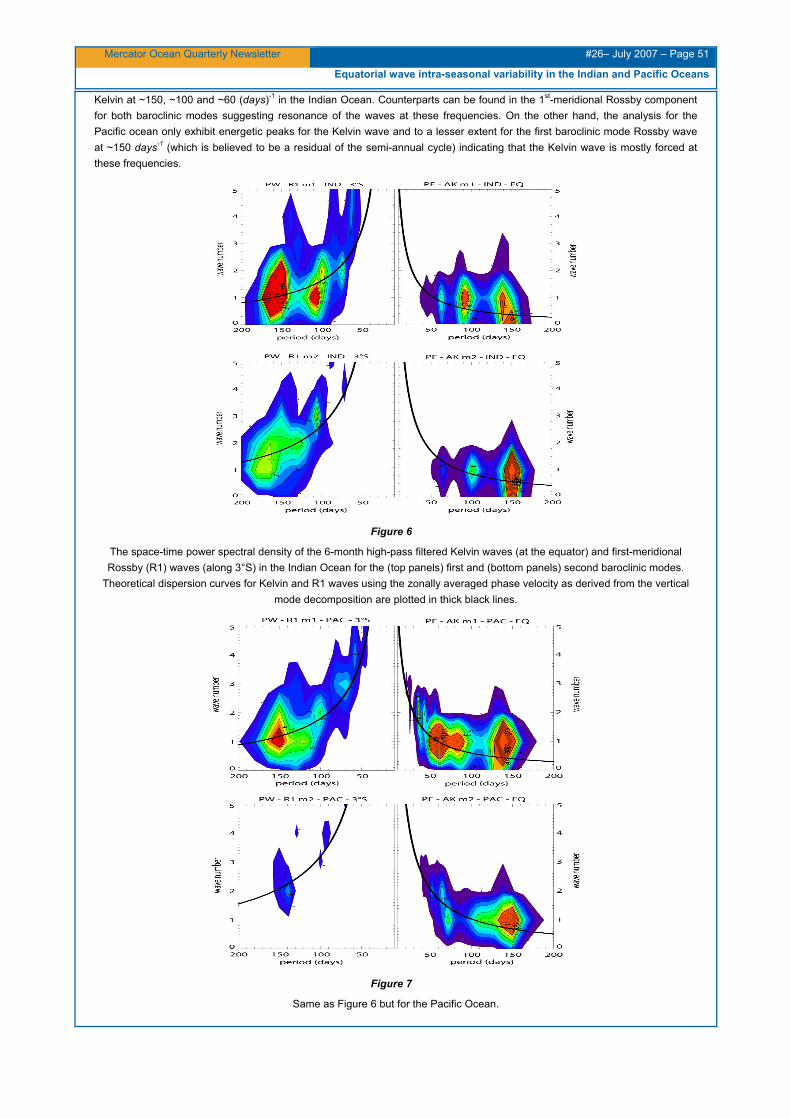
Mercator Ocean Quarterly Newsletter #26– July 2007 – Page 51
Equatorial wave intra-seasonal variability in the Indian and Pacific Oceans
Kelvin at ~150, ~100 and ~60 (days)-1 in the Indian Ocean. Counterparts can be found in the 1st-meridional Rossby component for both baroclinic modes suggesting resonance of the waves at these frequencies. On the other hand, the analysis for the Pacific ocean only exhibit energetic peaks for the Kelvin wave and to a lesser extent for the first baroclinic mode Rossby wave at ~150 days-1 (which is believed to be a residual of the semi-annual cycle) indicating that the Kelvin wave is mostly forced at these frequencies.
Figure 6
The space-time power spectral density of the 6-month high-pass filtered Kelvin waves (at the equator) and first-meridional Rossby (R1) waves (along 3°S) in the Indian Ocean for the (top panels) first and (bottom panels) second baroclinic modes.
Theoretical dispersion curves for Kelvin and R1 waves using the zonally averaged phase velocity as derived from the vertical mode decomposition are plotted in thick black lines.
Figure 7
Same as Figure 6 but for the Pacific Ocean.
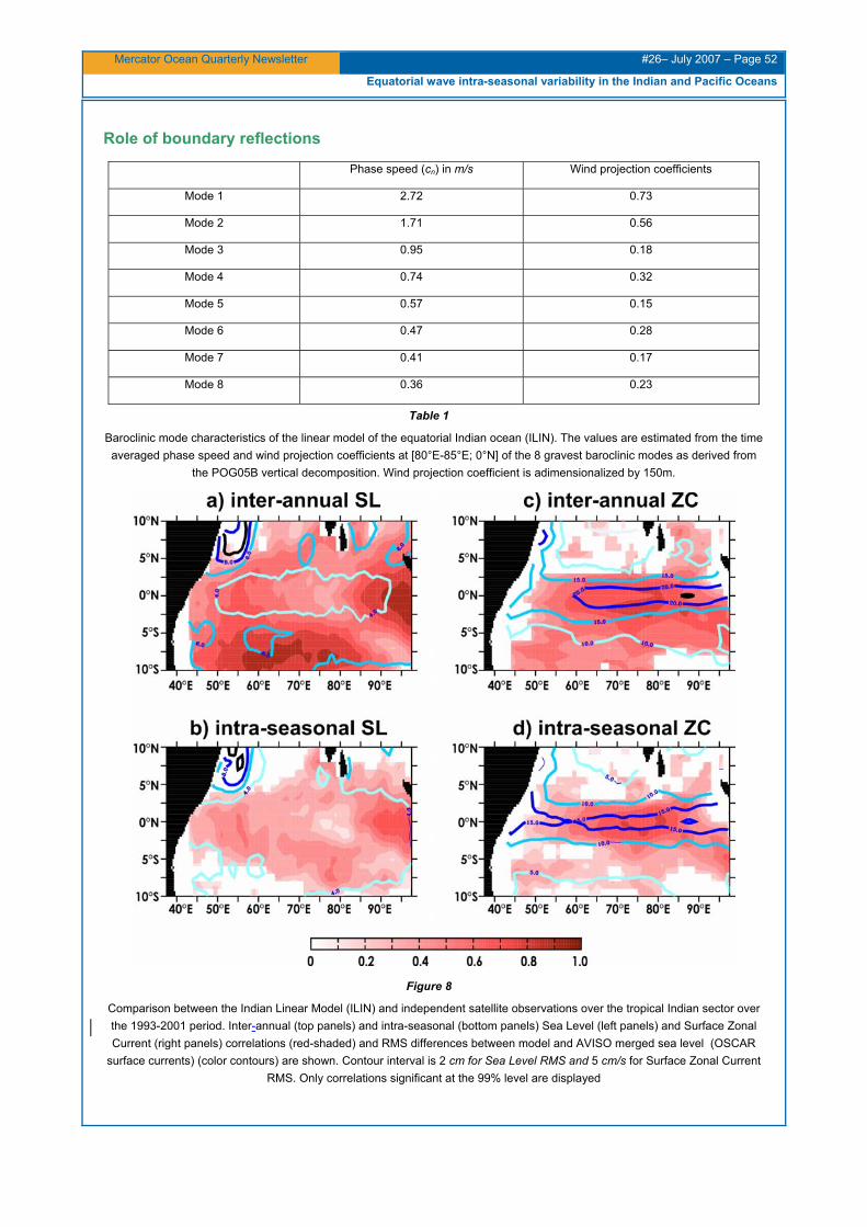
Mercator Ocean Quarterly Newsletter #26– July 2007 – Page 52
Equatorial wave intra-seasonal variability in the Indian and Pacific Oceans
Role of boundary reflections
Phase speed (cn) in m/s Wind projection coefficients
Mode 1 2.72 0.73
Mode 2 1.71 0.56
Mode 3 0.95 0.18
Mode 4 0.74 0.32
Mode 5 0.57 0.15
Mode 6 0.47 0.28
Mode 7 0.41 0.17
Mode 8 0.36 0.23
Table 1
Baroclinic mode characteristics of the linear model of the equatorial Indian ocean (ILIN). The values are estimated from the time averaged phase speed and wind projection coefficients at [80°E-85°E; 0°N] of the 8 gravest baroclinic modes as derived from
the POG05B vertical decomposition. Wind projection coefficient is adimensionalized by 150m.
Figure 8
Comparison between the Indian Linear Model (ILIN) and independent satellite observations over the tropical Indian sector over the 1993-2001 period. Inter-annual (top panels) and intra-seasonal (bottom panels) Sea Level (left panels) and Surface Zonal Current (right panels) correlations (red-shaded) and RMS differences between model and AVISO merged sea level (OSCAR
surface currents) (color contours) are shown. Contour interval is 2 cm for Sea Level RMS and 5 cm/s for Surface Zonal Current RMS. Only correlations significant at the 99% level are displayed

Mercator Ocean Quarterly Newsletter #26– July 2007 – Page 53
Equatorial wave intra-seasonal variability in the Indian and Pacific Oceans
A linear model of the Indian equatorial Ocean (hereafter ILIN) is designed taking advantage of the information provided by the vertical mode decomposition of POG05B.
The model is composed of 8 baroclinic modes with characteristics similar to POG05B (see Table 1). The model is validated from satellite observations (Figure 8), which indicates that it is as skilful as POG05B for simulating the surface current and sea level variability in the equatorial band (compare Figure 8 with Figures 1 and 2). This validates the results of the vertical mode decomposition presented above and allows for sensitivity tests with the model to study the role of equatorial waves at the meridional boundaries on the surface variability. In particular ILIN offers the opportunity to test the resonant character of the baroclinic modes. In the Indian Ocean, because of its narrow span, there is the possibility that intra-seasonal equatorial waves are forced through a resonance effect caused by stationary or slowly propagating patches of wind (Kessler et al., 1995). Cancelling out the reflection efficiency at the meridional boundary in ILIN will provide insight on such process. Such an experiment is carried out. Results are compared to the control experiment (i.e. considering full efficiency at the meridional boundary).
a) SZC [60°E-80°E, 2°S-2°N] b) mode 1 contribution
c) mode 2 contribution d) mode 3 contribution
Figure 9
Mean conservative spectrum [60°E-80°E, 2°S-2°N] of the ILIN Surface Zonal Current (SZC) estimated by autocorrelation for a) the total ZSC, b-d) the contribution of the 3 gravest baroclinic modes respectively. The plain black (dashed blue) line
respectively corresponds to the control experiment (‘no reflection’ experiment).

Mercator Ocean Quarterly Newsletter #26– July 2007 – Page 54
Equatorial wave intra-seasonal variability in the Indian and Pacific Oceans
a) R1 b) K reflected
c) K d) R1 reflected
Figure 10
Longitude-time plot of the second baroclinic mode contributions to the sea level anomalies simulated by the Indian Linear Model (ILIN): a) first meridional Rossby component (R1) at 3°S, b) reflected Kelvin wave contribution at 0°N, c) Kelvin wave
component (K) at 0°N and d) reflected R1 contribution at 3°S. R1 is displayed reverse from 99E to 43E in order to visualize the reflection at the western and eastern basin boundaries. Positive (negative) values are red (blue) shaded respectively.

Mercator Ocean Quarterly Newsletter #26– July 2007 – Page 55
Equatorial wave intra-seasonal variability in the Indian and Pacific Oceans
Figure 9 displays the spectrum of the simulated surface current anomalies in the central equatorial Indian Ocean. Figure 9a exhibits significant differences between the control experiment and the simulation without reflection at the boundary in particular at the frequencies ~180 and ~120, at which resonance is expected. The spectra of the gravest baroclinic mode contributions (figure 9b-d) show that the faster and less dissipative the baroclinic mode is, the more important the impact of the reflection at the meridional boundaries is. For the first and the second baroclinic modes (the most energetic), the impact on the intra-seasonal frequencies is significant: along with the specific resonance (120 and 180 days respectively) of each mode the reflection intensifies the wind energy in the intra-seasonal frequency band. For the high order baroclinic modes the impact becomes less noticeable.
The difference between both experiments allows estimating the contribution of the reflected Kelvin and Rossby waves (Figure 10). Although such estimate is dependent of some arbitrary choice on the dissipation coefficient (see Illig et al. (2004) for details), figure 10 suggests that the contributions of the reflected waves can reach the central basin with significant amplitude. Organized intra-seasonal wind forcing may then amplify the Kelvin wave at the resonant frequencies.
Discussion and conclusions
Equatorial waves in the Indian Ocean were clearly identified thanks to a vertical mode decomposition of the POG05B simulation. The analysis focuses on the intra-seasonal variability which is the dominant component of the surface variability in the Indian equatorial ocean. The results indicate that equatorial waves in the Indian Ocean have a significant contribution to the surface variability in terms of sea level and currents. The second baroclinic mode waves are the most energetic although the mean equatorial stratification favour the forcing of first baroclinic mode. The comparison with similar analysis over the equatorial Pacific ocean allows documenting the peculiarities of the results with respect to the nature of the wave (resonant versus forced). It is found that, whereas the intra-seasonal Kelvin wave is mostly forced by the wind in the Pacific Ocean, in the Indian Ocean, resonance of the waves takes place leading to energetic variability of the Rossby waves and surface current variability. Sensitivity experiments using a linear ocean model of the equatorial Indian Ocean support the above interpretation. The linear model is in particular as skilful as the OGCM for simulating the surface variability in the equatorial band supporting the interpretation of the variability in terms of long wavelength waves and resonance modes.
The issue of the relationship between intra-seasonal wind forcing and the equatorial oceanic Kelvin waves has drawn a lot of interest in recent years mostly because intra-seasonal variability in the western Pacific and Indian oceans is tightly link to ENSO triggering and development (Kessler et al., 1995). It has been suggested that this relationship must be strongly nonlinear because of the differing frequencies (Kutsuwada and McPhaden, 2002) but the nonlinear processes that couple these modes are not fully understood. The results reported here suggest that in the Indian equatorial ocean, superposition of linear waves with a specific vertical structure and their reflections at the meridional boundaries may explain the enhancement of the surface current variability at the resonant frequencies.
Overall, we have proposed and validated a methodology for deriving equatorial waves in the Indian Ocean using the POG05B Mercator-Ocean global simulation. Similar diagnostics applied to products with data assimilation based on the POG05B model version should bring further insights on the pertinence of our approach along with providing metrics of the impact of the assimilation, which in turn will allow resolving the scientific issues rose in this study.
Acknowledgements
We thank Eric Greiner for his support and for fruitful discussions during the course of this study.
References
Bonjean, F. and G. S. E. Lagerloef, 2002: Diagnostic model and analysis of the surface currents in the tropical Pacific ocean. J. Phys. Oceanogr., 32 (10), 2938–2954.
Boulanger J. P., and L.-L. Fu, 1996: Evidence of boundary reflection of Kelvin and first-mode Rossby waves from TOPEX/Poseidon sea level data. J. Geophys. Res., 101, 16 361–16 371.
Conkright, M. E., R. A. Locarnini, H. E. Garcia, T. D. O’Brien, T. P. Boyer, C. Stephens, and J. I. Antonov, 2002: World Ocean Atlas 2001: Objective Analyses, Data Statistics, and Figures [CD-ROM], NOAA, Silver Spring, Md.
Derval C, Durand E., Garric G. and E. Remy, 2005 : Dossier technique d'experimentation ORCA-R025 POG-05B , Mercator-Ocean internal report.
Dewitte B., G. Reverdin and C. Maes, 1999: Vertical structure of an OGCM simulation of the equatorial Pacific Ocean in 1985-1994.J. Phys. Oceanogr., 29, 1542-1570.

Mercator Ocean Quarterly Newsletter #26– July 2007 – Page 56
Equatorial wave intra-seasonal variability in the Indian and Pacific Oceans
Dewitte B., S. Illig, L. Parent, Y. duPenhoat, L. Gourdeau and J. Verron, 2003: Tropical Pacific baroclinic mode contribution and associated long waves for the 1994-1999 period from an assimilation experiment with altimetric data. J. Geophys. Research., 108 (C4), 3121-3138.
Ducet, N., P. Le Traon, and G. Reverdin, 2000: Global high resolution mapping of ocean circulation from Topex/Poseidon and ERS-1/2, J. Geophys. Res., 105, 19477-19498.
Handoh, I.C. and G.R. Bigg, 2000: A self-sustaining climate mode in the tropical Atlantic, 1995-1997: Observations and modelling, Q. J. R. Met. Soc., 126, 807–821.
Hayashi, Y., 1977: Space-time power spectral analysis using the maximum entropy method, J. Meteorol. Soc. Japan, 55, 415-420.
Illig S., B. Dewitte, N. Ayoub, Y. du Penhoat, G. Reverdin, P. De Mey, F. Bonjean and G.S. E. Lagerloef, 2004: Inter-annual Long Equatorial Waves in the Tropical Atlantic from a High Resolution OGCM Experiment in 1981-2000. J. Geophys. Research., 109, No. C2, C02022, doi:10.1029/2003JC001771.
Jakobsson, M., N.Z. Cherkis, and J.W.R.M.B. Coakley, (2000), New grid of Arctic bathymetry aids scientists and mapmakers., Eos, Transactions, American Geophysical Union, 81(9), 89-93-96.
Jourdan, D., E. Balopoulos, M.J. Garcia-Fernandez, and C. Maillard, Objective Analysis of Temperature and Salinity Historical Data Set over the Mediterranean Basin, (1998), IEEE.
Kessler, W. S., M. J. MacPhaden, and K. M. Weickmann, 1995: Forcing of intraseasonal Kelvin waves in the equatorial Pacific. J. Geophys. Res., 100, 10613-10631.
Kutsuwada, K., and M. McPhaden, 2002: Intraseasonal variations in the upper equatorial Pacific Ocean prior to and during the 1997-98 El Niño. J. Phys. Oceanogr., 32, 1133-1149.
Latif, M., D. Anderson, T. Barnett, M. Cane, R. Kleeman, A. Leetma, J. O'Brien, A. Rosati, and E. Schneider, 1998: A review of the predictability and prediction of ENSO. J. Geophys. Res., 103(C7), 14375-14393.
Le Blanc, J. L., and J. P. Boulanger, 2001: Propagation and reflection of long equatorial waves in the Indian Ocean from TOPEX/Poseidon data during the 1993–1998 period. Climate Dyn., 17, 547–557.
Levitus, S., T.P. Boyer, M.E. Conkright, T. OBrian, J.I. Antonov, C. Stephens, L. Stathopolos, D. Johnson, and R. Gelfeld, World Ocean Database 1998 - NOAA Atlas NESDID18, (1998), National Oceanographic Data Center, Silver Spring, MD.
Lythe, M., D.G. Vaughan, and B. Consortium, (2001), BEDMAP: a new ice thickness and subglacial topographic model of Antarctica., J. Geophys. Res., 106, 11335-11352.
Madec, G., P. Delecluse, M. Imbard, and C. Levy, OPA 8.1 general circulation model reference manual, (1998), Notes de l'Institut Pierre-Simon Laplace (IPSL) - Universite P. et M. Curie, B102 T15-E5, 4 place Jussieu, Paris cedex 5, 91p.
Madec, G., and M. Imbard, (1996), A global ocean mesh to overcome the North Pole singularity, Clim. Dyn., 12, 381-388.
Périgaud C. and B. Dewitte, 1996: El Niño-La Niña events simulated with the Cane and Zebiak’s model and observed with satellite or in situ data. Part I: Model and data comparison. J. Climate, 9, 66-84.
Shinoda, T., H. H. Hendon, and J. Glick, 1998: Intraseasonal variability of surface fluxes and sea surface temperature in the tropical western Pacific and Indian Oceans. J. Climate, 11, 1685-1702.
Smith, W.H.F., and D.T. Sandwell, (1997), Global sea-floor topography from satellite altimetry and ship depth soundings., Science, 277, 1956-1962.
Steele, M., R. Morley, and W. Ermold, (2001), PHC: A global ocean hydrography with a high quality Arctic Ocean., Journal of Climate, 14, 2079-2087.
Uppala, S., (2001), ECMWF Reanalysis, 1957-2001, ERA-40 - Proceedings of workshop Re-analysis, 5-9 november, ECMWF, Reading.
Xie, S.-P., and J. A. Carton, 2004: Tropical Atlantic variability: Patterns, mechanisms, and impacts. Earth Climate: The Ocean-Atmosphere Interaction, Geophys. Monogr., Vol. 147, Amer. Geophys. Union, 121–142.
Yuan D. and W. Han, 2006: Roles of Equatorial Waves and Western Boundary Reflection in the Seasonal Circulation of the Equatorial Indian Ocean, J. Phys. Oceanogr. 36, 930-944.
Mercator Ocean Quarterly Newsletter #26 – July 2007 – Page 57
Notebook
Notebook
Editorial Board :
Laurence Crosnier
Secretary :
Monique Gasc
Articles:
News1 : EGEE campaigns during the African monsoon multidisciplinary analysis program
By Bernard Bourlès
News2: Tropical arrays for observing ocean and atmosphere dynamics
By Fabrice Hernandez
The new 1/4° Mercator-Ocean global multivariate analysis and forecasting system: Tropical oceans outlook
By Marie Drévillon, Laurence Crosnier, Nicolas Ferry, Eric Greiner and the PSY3V2 Team
"Bulletin Climatique Global" of Météo-France; a contribution of Mercator-Ocean to the seasonal prediction of El Niño 2006-07
By Silvana Ramos Buarque , Christophe Cassou, Isabelle Charon and Jean-François Gueremy
Structure of intra-seasonal variability in the upper layers of the equatorial Atlantic Ocean from the Mercator-Ocean MERA-11 reanalysis
By Frédéric Marin, Gabriel Athié, Charly Régnier and Yves du Penhoat
Connexion between the equatorial Kelvin wave and the extra tropical Rossby wave in the South Eastern Pacific in the Mercator-Ocean POG05B simulation: a case study for the 1997/98 El Niño
By Boris Dewitte, Marcel Ramos, Oscar Pizarro and Gilles Garric
Equatorial wave intra-seasonal variability in the Indian and Pacific Oceans in the Mercator-Ocean POG05B simulation
By Serena Illig, Boris Dewitte, Claire Périgaud and Corinne Derval
Contact :
Please send us your comments to the following e-mail address: [email protected]
Next issue: October 2007