Mercator Ocean newsletter 25
40
Mercator Ocean Quarterly Newsletter #25 – April 2007 – Page 1 GIP Mercator Ocean Quarterly Newsletter Editorial – April 2007 Goce satellite Credits : ESA - AOES Medialab Greetings all, Nowadays, several datasets are -or will be- available in a near future to improve operational forecasting in most aspects, like the ocean dynamics modeling, and the assimilation efficiency, that aims now to optimize the combination of temperature/salinity in situ profiles, drifter's velocities, and sea surface height deduce from altimeter's data and GRACE or future Goce geoid. But also strengthen forecasting system's applications, like the climate monitoring. For all these issues, an optimal use of ocean data, always too sparse and not enough numerous, is mandatory. Such studies are at the heart of this Newsletter issue. It begins with a Rio M.H. and Hernandez F. review of the Goce Mission, dedicated to focus and document the shortest scales of the Earth's gravity field. Goce satellite is due to fly in December 2007. With the next article Guinéhut S. and Larnicol G. investigate the influence of the in situ temperature profiles sampling on the thermosteric sea level estimation. They show that the impact is not negligible, and can introduce large errors in the estimation. In the second article, Benkiran M. and Greiner E. are evaluating the benefits of the drifter's velocities assimilation in the Mercator Océan 1/3° Tropical and North Atlantic operational system. A description of the assimilation scheme upgrade to take into account velocity control is given. Castruccio F. & al. describe in the third article the performance of an improved MDT reference for altimetric data assimilation. They concentrate their study on the Tropical Pacific Ocean. Finally, the Newsletter comes to an end with the Benkiran M. article. In his study, based on the 1/3° Mercator system, the impact of several altimeters data on the assimilation performance is assessed Have a good read
-
Upload
mercator-ocean -
Category
Environment
-
view
123 -
download
0
Transcript of Mercator Ocean newsletter 25

Mercator Ocean Quarterly Newsletter 25 ndash April 2007 ndash Page 1
GIP Mercator Ocean
Quarterly Newsletter
Editorial ndash April 2007
Goce satellite Credits ESA - AOES Medialab
Greetings all
Nowadays several datasets are -or will be- available in a near future to improve operational forecasting in most aspects like the ocean dynamics modeling and the assimilation efficiency that aims now to optimize the combination of temperaturesalinity in situ profiles drifters velocities and sea surface height deduce from altimeters data and GRACE or future Goce geoid But also strengthen forecasting systems applications like the climate monitoring For all these issues an optimal use of ocean data always too sparse and not enough numerous is mandatory
Such studies are at the heart of this Newsletter issue It begins with a Rio MH and Hernandez F review of the Goce Mission dedicated to focus and document the shortest scales of the Earths gravity field Goce satellite is due to fly in December 2007 With the next article Guineacutehut S and Larnicol G investigate the influence of the in situ temperature profiles sampling on the thermosteric sea level estimation They show that the impact is not negligible and can introduce large errors in the estimation In the second article Benkiran M and Greiner E are evaluating the benefits of the drifters velocities assimilation in the Mercator Oceacutean 13deg Tropical and North Atlantic operational system A description of the assimilation scheme upgrade to take into account velocity control is given Castruccio F amp al describe in the third article the performance of an improved MDT reference for altimetric data assimilation They concentrate their study on the Tropical Pacific Ocean Finally the Newsletter comes to an end with the Benkiran M article In his study based on the 13deg Mercator system the impact of several altimeters data on the assimilation performance is assessed
Have a good read
Mercator Ocean Quarterly Newsletter 25 ndash April 2007 ndash Page 2
GIP Mercator Ocean
Contents
GOCE review 3
Data assimilation of drifter velocities in the Mercator Ocean system 6
Influence of the sampling of temperature data on the interannual variability of the global mean thermosteric sea level index 13
GRACE an improved MDT reference for altimetric data assimilation 20
Altimeter data assimilation in the Mercator Ocean system 32
Notebook 40
Mercator Ocean Quarterly Newsletter 25 ndash April 2007 ndash Page 3
News GOCE review
News GOCE review By Marie Heacutelegravene Rio1 and Fabrice Hernandez2
1 CLS Space Oceanography Division 810 rue Hermegraves 31520 Ranonville st Agne 2 Mercator Ocean 810 rue Hermegraves 31520 Ranonville st Agne
Satellite Altimetry and the Mean Dynamic Topography issue
Altimetric data from satellites are a key component of the observational constraints on which any operational ocean forecasting system can rely to ensure its ocean dynamics consistency The satellite altimeters offer global and repetitive measurements of the sea level with a unique resolution and accuracy Its success and accomplishment in ocean dynamics sciences is yet proven [eg Fu and Cazenave 2001]
However since the beginning of satellite altimetry more than 15 years ago due to the lack of an accurate geoid only the variable part of the ocean dynamic topography can be extracted with sufficient accuracy (few centimetres) for oceanographic applications For the correct interpretation of these altimetric Sea Level Anomalies (SLA) in terms of sea level and geostrophic circulation the provision of an accurate Mean Dynamic Topography (MDT) is mandatory This has proved to bring significant improvement in ocean forecasting systems where assimilation of SLA provides better ocean circulation description from large to mesoscales [Knudsen et al 2005 and EU GOCINA projects main outcomes Le Provost et al 1999 Le Traon et al 2002]
In addition the MDT is the missing key element for the correct interpretation of all past present and future altimetric data and their use for oceanographic long term analyses
Strong improvements have been made recently using satellite gravimetry products in particular the recent geoid models based on GRACE data Subtracting the last model EIGEN-GL4S computed by the GFZGRGS from an altimetric Mean Sea Surface allows computing the ocean Mean Dynamic Topography at scales larger than 400 km with accuracy of the order of few centimetres [Rio et al 2005 Tapley et al 2003]
But the MDT is expected to present scales as small as tenrsquos of km To retrieve the missing shortest scales different methods have been developed where in-situ oceanographic data (hydrologic profiles drifting buoy velocities) are combined with the large scale derived MDT to estimate global high resolution MDT [Niiler et al 2003 Rio and Hernandez 2004 Rio et al 2005 Rio et al 2007 Maximenko et al 2005]
However the definitive jump toward absolute altimetry is still to come and the springboard is called GOCE
GOCE mission
GOCE (Gravity Field and Steady-State Ocean Circulation) is the first core Earth Explorer mission from ESArsquos Living Planet programme and is due to fly in December 2007 The nominal duration of the mission is 20 months with a 3 month commissioning and calibration phase followed by two science measurement phases of 6 months separated by a 5 month eclipse hibernation period
Mission objectives are to determine the gravity fieldrsquos anomalies with an accuracy of 1 mGal (=10-5 ms2) and the Earth geoid with an accuracy of 1-2 cm for a spatial resolution of 100 km In order to meet these requirements the principle of the GOCE mission is based on the combination of two techniques a satellite to satellite tracking technique relative to GPS for retrieving the long wavelengths of the Earth Gravity field associated to the use of a gradiometer (composed of three pairs of three-axis accelerometers) for measuring the shortest scales
The two Level-2 products of interest for oceanographers that will be delivered by ESA are the set of spherical harmonics coefficients of the Earth gravity field up to degree and order 200 (100 km resolution) as well as the full error covariance matrix of the coefficients
GOCEGRACE complementarity
The GOCE satellite has been designed to focus on the retrieval of the Earthrsquos gravity field short scales while the previous GRACE US-German mission was designed to resolve with millimetre accuracy the spatial scales of the Earthrsquos gravity field longer than 400 km Both missions are then complementary so that the best static geoid model will certainly be obtained through a combination of gravity data from the two missions
The MDT solutions based on a combination of satellite and in-situ data mentioned above will play an important role for the validation of these future GOCEGRACE derived MDTs
Mercator Ocean Quarterly Newsletter 25 ndash April 2007 ndash Page 4
News GOCE review
Toward the shortest scales
GOCE data will give access with reasonable accuracy to the spatial scales of the ocean Mean Dynamic Topography larger than 100 km However in some areas (semi-enclosed seas as the Mediterranean Sea coastal areas straits) the MDT is expected to contain even shorter scales [Rio et al 2007] The combination methods to other independent estimates of the MDT based on in-situ oceanographic measurements will therefore still be essential to achieve higher resolution where needed Also in order to improve the geoid resolution local solutions can be computed combining GOCE data to in-situ (ship or airborne) gravimetric measurements
Opening new issues
Geoids accurate enough to be used together with satellite altimetry to provide a full description of the ocean mesoscale (10-1000km) have been expected for long time But the Russian dolls game is not over The access to the geoid short scales with a centimetric accuracy now pushes us toward the limits of altimetry This covers two key issues The first is the need to improve the accuracy of altimetric measurement in coastal areas through improved processing The second is to correctly assess the errors on the different models used for altimetric corrections in order to better understand at last what the true error levels on altimetric data (MSS SLA) are
Getting ready
Oceanographers have been used for years to work on altimetric Sea Level Anomalies focusing only to the ocean mesoscale variability The GOCE data will make us enter a new era where we will at last have access to the absolute dynamic topography and to the absolute ocean geostrophic currents not only for the forthcoming altimetric missions but also back in the past since the first altimetric measurements This will open a number of new scientific issues This will also have a huge impact for ocean and climate monitoring and forecasting and the operational forecasting centres must prepare from now to it thinking about the best way to assimilate this new information (the geoid and its error covariance matrix) into their systems
References
Fu L-L and A Cazenave Satellite Altimetry and Earth Sciences A handbook of Techniques and Applications 463 pp Academic Press San Diego CA USA 2001
Knudsen P OB Andersen R Forsberg AV Olesen AL Vest HP Foumlh D Solheim OD Omang R Hipkin A Hunegnaw K Haines RJ Bingham J-P Drecourt JA Johannessen H Drange F Siegismund F Hernandez G Larnicol M-H Rio and P Schaeffer GOCINA Geoid and Ocean Circulation in the North Atlantic pp 70 Danish National Space Center Copenhagen 2005
Le Provost C P Le Grand E Dombrowsky P-Y Le Traon M Losch F Ponchaut J Schroumlter BM Sloyan and N Sneeuw Impact of GOCE for ocean circulation studies ESA 1999
Le Traon P-Y F Hernandez M-H Rio and F Davidson How operational oceanography can benefit from dynamic topography estimates as derived from altimetry and improved geoid in ISSI workshop Earth gravity field from space - From sensors to Earth sciences Bern Switzerland Edited by G Beutler MR Drinkwater R Rummel and R von Steiger in Space and Science Reviews (108) pp 239-249 Kluwer Academic Publisher 2002
Maximenko NA and PP Niiler 2005 Hybrid decade-mean global sea level with mesoscale resolution In N Saxena (Ed) Recent Advances in Marine Science and Technology 2004 pp 55-59 Honolulu PACON International
Niiler PP NA Maximenko and JC McWilliams Dynamically balanced absolute sea level of the global ocean derived from near-surface velocity observations Geophys Res Lett 30 (22) 2164 doi1010292003GL018628 2003
Rio M-H and F Hernandez A Mean Dynamic Topography computed over the world ocean from altimetry in-situ measurements and a geoid model J Geophys Res 109 (C12) C12032 1-19 - doi1010292003JC002226 2004
Rio M-H Schaeffer P Hernandez F Lemoine J-M 2005 The estimation of the ocean Mean Dynamic Topography through the combination of altimetric data in-situ measurements and GRACE geoid From global to regional studies Proceedings of the GOCINA Workshop in Luxembourg (April 13-15 2005)
Rio M-H P-M Poulain A Pascual E Mauri G Larnicol and R Santoleri 2007 A Mean Dynamic Topography of the Mediterranean Sea computed from altimetric data in-situ measurements and a general circulation model J Mar Sys 65 (2007) 484-508
Mercator Ocean Quarterly Newsletter 25 ndash April 2007 ndash Page 5
News GOCE review
Tapley BD DP Chambers S Bettadpur and JC Ries Large scale ocean circulation from the GRACE GGM01 Geoid Geophys Res Lett 30 (22) 2163 doi1010292003GL018622 2003
Mercator Ocean Quarterly Newsletter 25 ndash April 2007 ndash Page 6
Data assimilation of drifter velocities in the Mercator Ocean system
Data assimilation of drifter velocities in the Mercator Ocean system By Mounir Benkiran and Eric Greiner1 1 CLS Mercator Ocean ndash 810 rue Hermegraves 31520 Ramonville st Agne
Introduction
The aim of this paper is to document the drifterrsquos velocities data assimilation in addition to other data already assimilated in the Mercator-Ocean system using a multivariate data assimilation scheme The latter has been upgraded and a new set of empirical modes have been defined which takes into account the drifter zonal and meridional velocities We describe here the various upgrades of the data assimilation system as well the first results from the drifter velocities data assimilation
The drifter velocities
For this study besides data used in the operational system (Sea Level Anomaly Temperature and salinity profiles and Sea Surface Temperature) we used the drifter velocity at 15 meters depth over the year 2004 Those are three days filtered which allows filtering the gravity waves
The PSY1v3 experimental system
We describe here the various upgrades of the data assimilation system in order to assimilate the drifter velocities The chosen experimental system (called PSY1v3) is a derived version of the 13deg Mercator-Ocean Tropical and North Atlantic operational system (PSY1v2) with an upgrade of the data assimilation scheme (formerly SAM1v2 and now called SAM1v3) in order to take into account the drifter velocity data in the state vector
The multivariate SAM1v2 data assimilation scheme is used operationally at Mercator-Ocean since early 2004 The model minus altimeter and insitu data differences of the multivariate analysis are performed using the SOFA (System for Ocean Forecasting and Analysis) optimal interpolation scheme (De Mey and Benkiran 2002 Etienne and Benkiran 2007) The specificity of the SOFA scheme is to split the horizontal and vertical correlations where the covariance matrix of the forecast error Br in the reduced space is described by
Br = S B ST = D 12 C D12
bull D the forecast error variance
bull B the forecast error
bull S the vertical modes (vertical correlation)
bull C the correlation function (as a fonction of the time-space correlation radius)
C = (1 + dr + 13 dr2) exp (-dr ) exp (-dt 2 )
The operational SOFA sequential data assimilation scheme (SAM1v2) allows assimilating sea level observations (derived from altimeter data sea level anomalies) sea surface temperature temperature and salinity vertical profiles and temperature and salinity climatological values The latter uses an optimal interpolation in a reduced space for which a statistical method based on empirical modes (EOFs) is used
The state vector is split into 2 parts a barotropic component (barotropic height) and a baroclinic component evaluated from temperature and salinity vertical profiles We first add the (U V) baroclinic velocity components in the state vector We then compute a new EOFs set with the new state vector X=[ψ T1hellipTjpkS1SjpkU1hellipUjpkV1hellipVjpk]T (where jpk is the total
number of vertical levels of the ocean model) including the new (U V) baroclinic velocity ψ is the barotropic stream function
The Ti Si Ui Vi variables are respectively the temperature salinity zonal and meridional velocity anomalies with respect to a seasonal mean at the corresponding i vertical level
Mercator Ocean Quarterly Newsletter 25 ndash April 2007 ndash Page 7
Data assimilation of drifter velocities in the Mercator Ocean system
In order to compute the new set of EOFs we use every 3 days instantaneous outputs of a one year long simulation for the year 2004 from the PSY1v2 system with double IAU1 (Incremental Update Analysis Ourmiegraveres amp al) IAU has been used to avoid every 7 days (length of the assimilation cycle) spikes in the analysis fields triggered by the sequential data assimilation scheme (Figure 1) Moreover in order to keep the seasonal cycle we compute a different set of EOF per season
We now have N vectors X corresponding to the N vertical profiles In order to compress the information containing the outputs variability using M vectors X (with M ltlt N) we express the vectors X in a new canonical orthonormal base S=en of dimension kz This base represents the directions along which the N profiles variances have a local extremum Hence we make sure using this method that two eigen modes are statistically not coupled and that the dominant modes are not coupled with the others
We then present which normalisation is applied to the state vector X composed of several ocean variables (ψ T S U V)
Indeed each of these variables has its own variability with different order of magnitude (typically of several degrees Celsius for the temperature or of the order of 025 psu for the salinity) Hence a normalisation is needed in order to extract the relevant dominating modes of the state vector The chosen normalisation method is not very different from the one used in the operational Mercator-Ocean system PSY1v2 It is based on a linearisation of the Bernoulli function A scaling is used so that each variable of the state vector becomes proportional to a sea level height The state vector is then described by the following equation
]1[ 1111 jpkpkjpkjpk dzdzdzjdzdzdzdzdzScale γγγγββαα=
minus= k levelat depth gravity to dueon accelaratienergy Kinetic
)0(2
exp exp
kk
k
ztgEcHztgEc
tcoefficienansionSalinitytcoefficienansionThermal
thicknessklayerdz
γ
βα
Figure 2 shows the percentage of explained variance by the first twenty mode in winter 2005 using the new state vector from the SAM1v3 scheme (left panel) and the old state vector from the SAM1v2 scheme (no IAU) (right panel) The new scheme allows increasing the percentage of explained variance with the same amount of eigen modes used The percentage of explained variance is ~100 everywhere except in the equatorial band where it reaches 92 This is due to the strong stratification present in the equatorial area which would require more than 20 modes to be fully represented Hence a test has been set up allowing using the right amount of mode at each grid point in order to explain 99 of the variance at each grid point
1 IAU refers to a more complex assimilation method than the classical sequential assimilation In the sequential method a forecast is followed by an analysis of the final conditions which once corrected become initial conditions for the next forecast With the IAU method instead of correcting the forecast initial condition the correction is spread along the integration period of the model The system state is thus modified while controlling its error IAU is a more complex and computer costly method as it requires an additional model integration Double IAU is a variant of the IAU which parameterises the model error using two analysis corrections weighted by sinusoidal complementary functions
Mercator Ocean Quarterly Newsletter 25 ndash April 2007 ndash Page 8
Data assimilation of drifter velocities in the Mercator Ocean system
Figure 1
Time series of the horizontal velocities divergence (cms) over the whole North and tropical Atlantic for 2004 (Red) with sequential data assimilation (Purple) in a free run without data assimilation (black) using Incremental Analysis Update
(IAU)
Figure 2
Explained variance for the first 20 modes during winter 2004 (Left panel) with SAM1v3 scheme (Right panel) with SAM2v1 scheme
Another originality of the SAM1v3 scheme lays in the correction applied to baroclinic velocities With the SAM1v2 scheme baroclinic velocities corrections are deduced from the 1st order thermal wind equation (and 2nd order in the equatorial band) Velocity corrections are deduced from the geostrophic increments derived from the temperature and salinity corrections In the SAM1v3 scheme baroclinic velocity corrections are now deduced from the statistical EOF projection in the reduced space This allows correcting the geostrophic as well as the ageostrophic component of the velocity Figure 3 displays the initialisation procedure used after the model analysis
Mercator Ocean Quarterly Newsletter 25 ndash April 2007 ndash Page 9
Data assimilation of drifter velocities in the Mercator Ocean system
Brest 12052006 Benkiran et al
SAM1v3 The Mercator Assimilation System version 3Schematically
ROOI (SOFA)
Delta (ir)r
δT δS
δUbac δVbac
δΨ
δU δV
δUbar δVbar
baroclinic
barotropic
Full space
1D EOFs
Static instabilityof the water column
Sets to 0 the divergentpart of the current
baroclinic
Figure 3
Initialisation procedure after analysis in the SAM1v3 scheme
Preliminary results comparison of the SAM1v2 and SAM1v3 data assimilation schemes and impact of drifterrsquos velocities data assimilation in the SAM1v3 system
We present here preliminary results first comparing the SAM1v2 and SAM1v3 data assimilation schemes and second showing the impact of drifter velocities data assimilation in the SAM1v3 system
First the SAM1v2 and v3 schemes are compared with no drifter velocity data assimilation Two simulations in the exact same conditions have been performed in order to assess the differences between the SAM1v2 and SAM1v3 schemes Simulations are performed for the year 2004 when enough data are available assimilating the same observations (Jason Envisat and Gfo for altimeter data Coriolis temperature and salinity vertical profiles Reynolds Sea Surface Temperature) Alimeter data from a fourth satellite (Topex) are also available as independent observations Figure 4 shows the biases between the Topex observations and the model The Root Mean Square (RMS) (Top panel) is lower for SAM1v3 than in SAM1v2 scheme This is mainly due to the ageostrophic velocity corrections Moreover the biases averages (lower panel) are close to zero in both schemes
Figure 5 compares the Sea Surface Temperature (SST) forecasted by the model and the Reynolds SST which is assimilated We notice that the biases are reduced in SAM1v3 compared to v2 especially close to the continental shelf in the Gulf Stream and the Caribbean areas Figure 6 shows that this is mostly due to the ageostrophic velocity correction applied in SAM1v3 Indeed in the SAM1V2 scheme only the barotropic and geostrophic baroclinic velocities are corrected This does not allow the current to develop on the continental plateau Figure 6 shows the mean velocities in the North West Atlantic in the two schemes The Greenland Current feeding the Labrador Current is more developed on the continental shelf with SAM1v3 than v2 scheme
Mercator Ocean Quarterly Newsletter 25 ndash April 2007 ndash Page 10
Data assimilation of drifter velocities in the Mercator Ocean system
Figure 4
(Top panel) RMS of the biases (cm) between Topex and model in the 7 days forecast fields over the whole tropical and North Atlantic domain (Lower panel) Misfit average (cm) Blue line With no altimeter data assimilation Brown line SAM1v3 with
altimeter data assimilation (Envisat Jason and Gfo) Black line SAM1v2 with altimeter data assimilation (Envisat Jason and Gfo)
Figure 5
SST biases (Unit [-15-15] degC)between the model forecast and the assimilated Reynolds SST (Left) with SAM1V2 (right) with SAM1V3
Mercator Ocean Quarterly Newsletter 25 ndash April 2007 ndash Page 11
Data assimilation of drifter velocities in the Mercator Ocean system
Figure 6
Mean current (ms) for year 2004 (Left panel) with SAM1V2 (right panel) with SAM1V3
Figure 7
Drifters buoys trajectories during year 2004 in the tropical and North Atlantic (Right) zonal (left) meridional component
Second the SAM1v3 scheme is used to assimilate drifterrsquos velocities A simulation is performed where only drifterrsquos velocities data are assimilated every 7 days over the year 2004 Drifterrsquos data are available daily but treated with a 3 days filter We first want to check whether our new set of EOFs is compatible with the drifterrsquos velocities data Moreover we want to check which error is associated with these data and which impact it will have on the system once assimilated
Figure 7 shows the drifterrsquos buoys trajectories during 2004 in the tropical and North Atlantic Zonal equatorial currents as well as stronger currents in the Gulf Stream area can be noticed
Figure 8 displays the sum of the forecast differences between the model and the drifter data for the zonal component of the velocity (left panel) as well as the sum of the increments after analysis for the zonal component of the velocity (right panel) We notice that the information contained in the drifterrsquos data is not use at 100 but that only a small part of it is used in the whole domain except in the tropical area where corrections are larger We suggest some reasons for this
bull The observation error associated with the drifter data is constant over the whole basin (010 ms) We made a test with a weaker error (5 cms not shown here) where more mesoscales structures are kept
bull The new set of EOFs released within the SAM1v3 scheme might not include the drifter data signal although the zonal and meridional components of the velocity have been included in the state vector
bull The optimal interpolation scheme used here with a vertical projection as well as the resolution of the system might not be compatible with the mesoscale structures present in the drifterrsquos data
bull As these data are 3 days filtered we should also filter the model equivalent in order to filter the model gravity wave This is not done in this study and will be done in future work
Mercator Ocean Quarterly Newsletter 25 ndash April 2007 ndash Page 12
Data assimilation of drifter velocities in the Mercator Ocean system
Figure 8
(Left panel) Sum of the forecast differences (ms) between the model and the drifterrsquos data for the zonal component of the velocity (Right panel) Sum of the increments (ms) after analysis for the zonal component of the velocity
Conclusion
This study allowed us to conclude on the following points
bull It is important to use the baroclinic component of the velocity in the state vector It adds an ageostrophic correction to the velocity after analysis which is not taken into account when this correction is simply inferred from the thermal wind equation
bull This first experiment of drifter velocity data assimilation in Mercator Ocean System gave us encouraging preliminary results Further work and improvements are needed and will be conducted in order hopefully to reach better results
References
De Mey P and M Benkiran 2002 A multivariate reduced-order optimal interpolation method and its application to the Mediterranean basin-scale circulation Ocean Forecasting Conceptual basis and applications N Pinardi Springer-Verlag Berlin Heidelberg New York 281-306
Etienne H and M Benkiran 2007 Multivariate assimilation in MERCATOR project new statistical parameters from forecast error estimation Journal of Marine Systems 65 430-449
Ourmiegraveres Y J M Brankart L Berline P Brasseur amp J Verron in press Incremental analysis update implementation into a sequential ocean data assimilation system Journal of Atmospheric and Oceanic Technology
Acknowledgment
Laurence Crosnier is greatly acknowledged for the translation of this paper
Mercator Ocean Quarterly Newsletter 25ndash April 2007 ndash Page 13
Influence of the sampling of temperature data on the interannual variability of the global mean thermosteric sea level index
Influence of the sampling of temperature data on the interannual variability of the global mean thermosteric sea level index By Steacutephanie Guinehut and Gilles Larnicol1
1 CLS Space Oceanography Division 810 rue Hermegraves 31520 Ranonville st Agne
Introduction
Global mean sea level change results from two main causes (1) volume change due to seawater density change in response to temperature and salinity variations (2) mass change due to exchange of water with atmosphere and continents via the hydrological cycle Satellite altimeters measure global mean sea level including volume and mass changes almost globally (60degS-60degN) and continuously since the launch of TopexPoseidon in October 1992 In situ temperature and salinity data sets are used to quantify volume change due to temperature change (thermosteric sea level ndash heat content) and temperature and salinity change (steric sea level)
Different groups have recently estimated interannual variability of global ocean heat content and global ocean thermosteric sea level change for the 1993-2006 periods (Willis et al 2004 Ishii et al 2006 Lyman et al 2006) Unfortunately in situ measurements are discrete in time and space and are far from sampling the total surface of the ocean The main objective of this study is thus to quantify the sampling influence of the temperature data sets on the interannual variability of the global mean thermosteric sea level Sampling errors depend on three components 1) the geographical and temporal repartition of the in situ measurements 2) the vertical resolution of the measurements and 3) the method used to calculate global mean from non-global observations The influence of these three terms has been quantified and their impacts in terms of global trend of interannual variability of the global mean thermosteric sea level are thus presented
The different data sets involved in this study are first presented in section 2 The method used to map the individual temperature observations into grid fields is then described in section 3 The impact of the temporal geographical and vertical repartition of the in situ measurements is studied in section 4 and the impact of the method used to calculate the global mean from non-global fields is presented in section 5 Finally section 6 offers discussions
Data sets
Data sets involved in this study include
bull Delayed mode maps of SLA from the SSALTODUACS center (SsaltoDuacs User Handbook 2006) These maps are defined on a 13deg horizontal grid at a weekly period
bull T and S in situ profiles from the ENACTENSEMBLE-EN2 data base for the years 1993-2004 (Ingleby and Huddleston 2006) ndash the third upgrade of the data set (EN3) was unfortunately not available at the time of the study
bull T and S in situ profiles from the CORIOLIS data base for the years 2005-2006 (httpwwwcorioliseuorg)
The preprocessing of the in situ data sets consists only in removing redundant observations ndash only one observation is kept per day for the same instrument in a region of 01deg in latitude by 01deg in longitude No additional qualification is performed on the observations we absolutely rely on the data centers for this particular point
Mapping method
In situ data sets being discrete measurements in time and in space a mapping method is used prior to analysis We construct global thermosteric sea level maps at a monthly period on a 13deg resolution grid and for the 0-700 m layer from the individual temperature profiles The mapping method is very similar to the one developed by Larnicol et al (2006) for the ARMOR-3D Mercator observed products It is based on an optimal interpolation method with the following parameters
bull Temporal correlation scale of 45 days
bull Spatial correlation scale ndash 5 times the one used to produce the SSALTODUACS SLA maps (from 1500 km at the equator to 700 km at 50degN)
bull Error associated to each in situ measurement as thermosteric sea level equal to 20 of the variance of the SSALTODUACS SLA maps in order to take into account error associated to the aliasing of the mesoscale variability
Besides the time-mean and seasonal cycle were removed from the altimeter and in situ data prior to analysis
Mercator Ocean Quarterly Newsletter 25ndash April 2007 ndash Page 14
Influence of the sampling of temperature data on the interannual variability of the global mean thermosteric sea level index
Impact of the temporal geographical and vertical repartition of the in situ measurements
Each observation being characterised by a geographical position (latitude and longitude) and a date the temporal and geographical repartition of the in situ measurements could not be studied independently of one another The vertical sampling of the in situ observations is studied in a second step Figure 1 shows three typical repartitions of in situ temperature profiles valid up to 700 m (the thermosteric sea level is calculated down to 700 m) The year 1993 shows medium repartition of the in situ measurements with large under-sampled areas in the Southern Ocean As we will see later we are able to reconstruct almost 85 of the ocean thermosteric signal between 60degS and 60degN (the area of the study) for this year For the year 2000 very large areas in the Indian Ocean the South Atlantic and Pacific Oceans are hardly sampled if at all This year is the worst sampled year with only 70 of the ocean reconstructed Thanks to the development of the Argo array the ocean is almost totally sampled during the year 2006 with more than 95 of the 60degS-60degN area reconstructed
Impact of the temporal and geographical sampling - Method
Errors on the global ocean thermosteric sea level have been estimated in a very similar way as in Lyman et al (2006)
bull Annual mean reference fields are computed from weekly SSALTODUACS SLA maps for the years 1993-2005
bull For each of these 13 annual mean SLA reference fields 144 (12 months x 12 years from 1993 to 2004) monthly sets of simulated observations are created by sub sampling the reference fields at the time and position of the in situ temperature profiles
bull Monthly SLA maps are next reconstructed for each of the 13x144 sets of simulated observations The mapping method used is the one described in section 0
bull Finally differences between the reconstructed fields and the reference fields as global averages for the 60degS-60degN area are calculated for the 1993-2004 periods and for each of the 13 realizations Errors in the global thermosteric sea level are calculated from the rms over the 13 realizations
Figure 1
Number of in situ temperature profiles valid up to 700-meter depth in 1degx1deg boxes for the year 1993 2000 and 2006 Color scale from 2 to 18 every 4
Mercator Ocean Quarterly Newsletter 25ndash April 2007 ndash Page 15
Influence of the sampling of temperature data on the interannual variability of the global mean thermosteric sea level index
Two tests have been performed using this method For the first test (test 1) the global mean (between 60degS and 60degN) is calculated from the reconstructed areas ndash the mean is thus sometimes far from being global (Figure 2) For the second test (test 2) the reconstructed fields are first completed by zero values in order to create global fields before the calculation of the global mean As we will see large differences between test 1 and test 2 can appear because of large-unreconstructed area in very poor sampled years (Figure 2)
Figure 2
Annual mean reference SLA field for the year 1993 (left) and monthly reconstructed field for January 2000 obtained using the mapping method of the sub sampled 1993 reference field at the January 2000 observations (right) Color scale from -10 to 10
every 1 cm
Impact of the temporal and geographical sampling ndash Results
Results indicate that errors associated to the global mean thermosteric sea level vary from one year to another as a function of the temporal and geographical repartition of the in situ measurements and thus as a function of the percentage of reconstructed ocean (Figure 3 Figure 4) The percentage of reconstructed ocean is calculated by comparing the area of the ocean reconstructed by the mapping method using the in situ observation (area in colour on Figure 2-right) to the area sampled by the reference field (Figure 2-left) between 60degS and 60degN
Results also indicate that errors quite differ between test 1 (uncompleted field) and test 2 (field completed by zero values) For test 1 errors vary from 009 cm rms for well sampled years (1995 2004 for example) to 017 cm rms for less well sampled years (2000 2001) Errors are much larger for test 2 and vary from 010 cm rms for the year 2004 which is well sampled with more than 95 of the ocean reconstructed to 044 cm rms for the year 2000 which is really less well sampled with only 70 of the ocean reconstructed
It is therefore really difficult to evaluate the true errors associated to the global mean thermosteric sea level We think nevertheless that test 1 minimizes the error since it assumes that the missing field is centred on zero and that test 2 maximizes the errors since it assumes that the missing field is everywhere equal to zero The truth errors might thus be situated between the green and the bleu curves on Figure 3 They might vary from 01 cm rms for a well sampled ocean and between 017 and 044 cm rms when the ocean is less well reconstructed
Additionally a clear linear relationship is observed between the error on the global mean thermosteric sea level and the percentage of the reconstructed ocean (Figure 4) This linear relationship is a very powerful tool to infer the error as a function of the geographical repartition of the in situ measurements and to anticipate and emphasis the need of new in situ observations in term of array design experiment Results indicate also that the errors can be very high (from 05 cm rms to 15 cm rms) in area with just a few in situ measurements and for which the percentage of reconstructed ocean is very low (lt10 )
Of course these results are also attached to the mapping method used There is a compromise between the mapping method which smoothes the individual observations onto a spatially consistent field and the temporal and spatial repartition of the in situ observations
Mercator Ocean Quarterly Newsletter 25ndash April 2007 ndash Page 16
Influence of the sampling of temperature data on the interannual variability of the global mean thermosteric sea level index
Figure 3
Monthly rms error on global mean thermosteric sea level for the period 1993-2004 (cm) Green curve test 1 (see text) Blue curve test 2 Turquoise curve percentage of reconstructed ocean for the area 60degS-60degN The dotted lines correspond to 12-
month averages
Figure 4
Rms error on global mean thermosteric sea level as a function of percentage of reconstructed ocean (cm) Green curve test 1 (see text) Bleu curve test 2
Impact of the vertical sampling
The impact of the vertical sampling of the in situ measurements is also studied as it varies as a function of probe type and thus as a function of time
High-resolution XBT and CTD measurements have usually 1-dbar vertical resolution from top to bottom as low-resolution CTD have very dispersed vertical sampling characteristics and as profiling float measurements have roughly 10-dbar vertical resolution near the surface and wider resolution at depth for a mean number of 80 observations between the surface and 2000-meter depth Simple statistics calculated for the top 700-meter depth and for the 1993-2006 period show that the mean vertical interval between two measurements was between 10-dbar and 15-dbar at the beginning of the period that it increased to 20-dbar for the year 2000 and up to 30-dbar for the year 2003 After this year it decreased to 15-dbar with the development of profiling float measurements The depth of the first measure at the surface has also deepened from 2-dbar from 1993 to 2002 to 4-dbar since the coming of profiling float measurements
Mercator Ocean Quarterly Newsletter 25ndash April 2007 ndash Page 17
Influence of the sampling of temperature data on the interannual variability of the global mean thermosteric sea level index
In order to quantify the impact of the vertical sampling of the in situ measurements on the interannual variability of the global mean thermosteric sea level global temperature and salinity fields from the global PSY3v1 Mercator system (Dreacutevillon et al 2006) are used The fields used are the one publicly available and re-interpolated every 5-meter in the top 30 meters then every 10 to 15-meters down to 75-meters and then every 25-meters down to 700-meters
The method consists in interpolating the PSY3v1 fields at the position of the in-situ measurements using two vertical interpolation procedures 1) keeping the vertical resolution of the PSY3v1 system 2) interpolating the PSY3v1 temperature and salinity fields on the in-situ z-levels The two sets of synthetic observations are then used to calculate global mean thermosteric sea level Results (not showed) indicate that the vertical sampling of the in situ measurements have no significant impact on the results which means that the past and actual vertical sampling of the in situ measurements are suitable to study climate signals
Impact of the method used to calculate global mean thermosteric sea level
Results presented in section 0 show that errors on the global mean thermosteric sea level due to sampling characteristics of the in situ measurements present values which vary as a function of the temporal and geographical repartition of the in situ measurements but also as a function of the method used to calculate the global mean thermosteric sea level (fields completed or not before the calculation of the global mean)
Three tests have been performed in order to quantify the errors associated to the method used to calculate the global mean thermosteric sea level calculated from the in situ observations As the geographical repartitions of the in situ measurements are not global they donrsquot allow the calculation of a ldquotruerdquo global mean of the thermosteric fields An important question is thus to know if it is necessary or not to complete the thermosteric field before the calculation of the global mean and if the answer is yes with what values
Three tests have thus been performed in order to calculate global mean thermosteric sea level
bull Test 1 from non global in situ mapped fields
bull Test 2 from global in situ mapped fields completed by the time-mean field (ie Levitus annual mean climatology) which is a static field during the whole period
bull Test 3 from global in situ mapped fields completed by ldquostericrdquo altimeter SLA fields which are time-variable fields The ldquostericrdquo altimeter SLA fields are deduced from regression coefficients computed from a global altimeter (SLA) in situ (steric-height) comparison study (Guinehut et al 2006)
Figure 5
Global mean thermosteric sea level for the three tests black green and blue curves (see text) (in cm) The turquoise curve corresponds to the percentage of reconstructed ocean for the area 60degS-60degN Thick lines correspond to 12-month running
mean
Mercator Ocean Quarterly Newsletter 25ndash April 2007 ndash Page 18
Influence of the sampling of temperature data on the interannual variability of the global mean thermosteric sea level index
The three tests show quite similar results (Figure 5) The global tendencies are very close but the associated trends can be relatively different Results are sensitive to the method used to complete or not the fields particularly when the percentage of reconstructed ocean are lower like during the years 2000 and 2001 Differences between the three tests can then be of the order of 05 cm for percentage of reconstructed ocean of 70
The values are completely coherent with the ones presented on Figure 4 They show additionally that upper bound values presented on Figure 4 are totally realistic It is obviously almost impossible to tell if one estimation of the global mean thermosteric sea level is more realistic than the others but this study helps to understand the dispersions observed between the different published estimates (see for example httpsealevelcoloradoedustericphp for a review)
Discussion
Additionally to other uncertainty related to measurements accuracybias for example error bars on the global mean thermosteric sea level due to sampling characteristics of the in situ measurements vary as a function of temporal and geographical repartition of the in situ measurements but also and coherently as a function of the method used to calculate the global mean thermosteric sea level (fields completed or not and with what values before the calculation of the global mean)
As it has been specified in section 0 no additional qualification has been performed on the in situ temperature measurements An important notice has been recently made to Argo data users rising pressure offset errors on SOLO floats equipped with FSI CTD The consequence was the introduction of a significant cold bias in the analyses by these instruments (Figure 6) At the same time there are lots of discussions concerning XBT measurements which are the primary source of the data used in the different studies on thermosteric sea level interannual variability Some published (Gouretski and Koltermann 2007) or ongoing studies (Wijffels et al in prep) have recently showed that XBT measurements exhibit warm bias of the order of 04 et 05 degC on the water column around 100-meter depth by comparison to other data sets resulting in depth-averaged values from 01degC in the 90s to 03degC in 2000-2001 (Gouretski and Koltermann 2007) The warm bias suspected at the beginning of the period of the study combined to the cold bias due to some Argo float measurements problem suggest that care much be taken when using simultaneously all these data sets and when interpreting the results Results by Lyman et al (2006) have for example recently been revisited by Willis et al (2007) and they demonstrate that the recent cooling signal in the upper ocean (as the one presented on Figure 6) is an artifact of the simultaneous use of Argo floats and XBT measurements and that the introduced biases are larger than the sampling errors Results showed on Figure 6 must then be taken cautiously
Figure 6
Interannual variability of the global mean altimeter sea level (black curve) and thermosteric sea level calculated with all available in situ temperature measurements valid up to 700-meter depth (blue curve) and calculated with all available temperature
measurements except the SOLO-FSI floats data (green curve) (in cm) Error bars are from Figure 4 and Figure 5 The turquoise curve corresponds to the percentage of reconstructed ocean for the thermosteric estimation and for the area 60degS-60degN the
dash line corresponding to the no SOLO-FSI case
Mercator Ocean Quarterly Newsletter 25ndash April 2007 ndash Page 19
Influence of the sampling of temperature data on the interannual variability of the global mean thermosteric sea level index
There are thus very strong needs for careful and precise validationcalibration of the different in situ data sets Uncertainties still persist on different points including fall rate equation of the XBT measurements coarse automated quality control procedure on real-time profiling float data salinity drifts on profiling float instruments
In spite of these reserves the Argo almost global profiling float array now offers the opportunity to study deeper thermal contributions than 700-meters but also the impact of salinity field on sea level interannual variability Additionally studies using independent data sets like GRACE measurements which provide estimates of mass change must be carried on (see for example Lombard et al 2006) in order to close the sea level budget
References
Dreacutevillon M Y Drillet G Garric J-M Lellouche E Reacutemy C Deval R Bourdalleacute-Badie B Tranchant M Laborie N Ferry E Durand O Legalloudec P Bahurel E Greiner S Guinehut M Benkiran N Verbrugge E Dombrowsky C-E Testut L Nouel F Messal 2006 The GODAEMercator global ocean forecasting system results applications and prospects World Maritime technology conference proceedings
Gouretski V and K P Koltermann 2007 How much is the ocean really warming Geophys Res Lett 34 L01610 doi1010292006GL027834
Guinehut S P-Y Le Traon and G Larnicol 2006 What can we learn from Global AltimetryHydrography comparisons Geophys Res Lett 33 L10604 doi1010292005GL025551
Ingleby B and M Huddleston 2006 Quality control of ocean temperature and salinity profiles - historical and real-time data To appear in Journal of Marine Systems
Ishii M M Kimoto K Sakamoto and SI Iwasaki 2006 Steric sea level changes estimated from historical ocean subsurface temperature and salinity analyses Journal of Oceanography 62 (2) 155-170
Larnicol G S Guinehut M-H Rio M Drevillon Y Faugere and G Nicolas 2006 The Global Observed Ocean Products of the French Mercator project Proceedings of 15 Years of progress in Radar Altimetry Symposium ESA Special Publication SP-614
Lombard A D Garcia G Ramillien A Cazenave R Biancale JM Lemoine F Flechtner R Schmidt and M Ishii 2006 Estimation of steric sea level variations from combined GRACE and Jason-1 data submitted to EPSL
Lyman JM JK Willis and GC Johnson 2006 Recent Cooling of the Upper Ocean Geophys Res Lett 33 (18 L18604)
SsaltoDuacs User Handbook 2006 (M)SLA and (M)ADT Near-Real Time and Delayed Time Products SALP-MU-P-EA-21065-CLS Edition 15
Willis JK D Roemmich and B Cornuelle 2004 Interannual variability in upper ocean heat content temperature and thermosteric expansion on global scales J Geophys Res 109 (C12036 doi1010292003JC002260) 13
Willis JK JM Lyman GC Johnson and J Gilson 2007 Correction to ldquoRecent Cooling of the Upper Ocean Geophys Res Lett submitted
Mercator Ocean Quarterly Newsletter 25ndash April 2007 ndash Page 20
GRACE an improved MDT reference for altimetric data assimilation
GRACE an improved MDT reference for altimetric data assimilation By Freacutedeacuteric Castruccio1 Jacques Verron 1 Lionel Gourdeau2 Jean Michel Brankart1 and Pierre Brasseur1 1 Laboratoire des Ecoulements Geacuteophysiques et Industriels BP 53 38041 Grenoble Cedex 9 2 IRD Institut de recherche pour le deacuteveloppement BP A5 98848 Noumeacutea cedex Nouvelle-Caleacutedonie
Introduction
Since 1992 the altimetric satellites provide a high precision high resolution and quasi-synoptic observation of the Sea Surface Height (SSH) the sea level above a reference ellipsoid The SSH signal is the sum of (i) the geoid and (ii) the dynamic topography Only the later is relevant for oceanographic applications However the poor knowledge of the geoid has prevented the oceanographers to fully exploit the altimetric measurement and altimetric applications have concentrated on ocean variability through the analysis of the Sea Level Anomaly (SLA) The SLA has been widely and successfully used to improve our knowledge of the ocean dynamics [Fu and Cazenave 2001] Nevertheless it is still challenging to infer the ocean dynamic topography (DT) from the altimetric signal because of geoid uncertainties Absolute Dynamic Topography have only been accessible by the addition of a Mean Dynamic Topography (MDT) estimate to the SLA
In the context of altimetric data assimilation the definition of a reliable MDT reference is a recurrent issue [Blayo et al 1994 Birol et al 2004] A variety of methods have been applied to generate MDT products but none of them was found fully satisfactory
Several geodetic missions like CHAMP (2000) GRACE (2002) and GOCE scheduled for 2007 are dedicated to provide a precise estimate of the ocean geoid (with a centimetric precision for short-wavelength features around 100 km) Several studies have recently concluded that the actual resolution of the MDT reference computed using gravimetric data is now compatible with the use in a context of data assimilation experiments [Gourdeau et al 2003] in particular in the tropical Pacific Ocean which is our region of interest
The objective of this study is to investigate the impact of a mean dynamic topography deduced from a GRACE geoid on the assimilation of altimetric data along with in-situ temperature profiles The emphasis is on the better compatibility between both types of observation data sets This better mean state compatibility contributes to provide a more efficient data assimilation making a better use of the data complementarity The results are promising and represent a clear improvement regarding previous studies [eg Parent et al 2003] Nevertheless some limitations persist most of them related to the resolution of the geoid
The investigation is performed with a primitive equation model of the tropical Pacific Ocean where an easily accessible and rather synoptical set of in-situ data is available thanks to the TAOTRITON moorings to complement the altimetric observations The Singular Evolutive Extended Kalman (SEEK) filter is used to jointly assimilate the TOPEXPOSEIDON and ERS1amp2 SSH referenced to the GRACE geoid and the TAOTRITON temperature profiles Two 6-year hindcast experiments over the 1993-1998 period encompassing the strong 1997-1998 El NintildeoLa Nintildea event have been performed They only differ by the use of data assimilation
This note is divided in 5 sections Following introduction the model the assimilation scheme and the assimilated data are described in section 2 Section 3 is dedicated to the mean sea surface reference issue and the so-called GRACE MDT used to reference altimetric residual component Results of the 6-year hindcast experiment are analyzed in section 4 Section 5 discusses and summaries the results
Assimilation Experiment model method and data sets
Model
The assimilation experiments were performed with the OPA1 OGCM The configuration is the so-called ORCA2 configuration a global low resolution 2degx2deg ORCA type grid [Madec et Imbard 1996] with a variable meridional resolution varying from 05deg at the equator to 2deg poleward of 20deg in latitude in order to improve the equatorial dynamics The model solves the primitive equations of ocean dynamics and use a free surface formulation [Roullet and Madec 2000] The temporal scheme is a leap-frog scheme with a 5760 seconds time step Along the vertical there are 31 z-coordinate levels This model has been used
1httpwwwlodycjussieufrNEMO
Mercator Ocean Quarterly Newsletter 25ndash April 2007 ndash Page 21
GRACE an improved MDT reference for altimetric data assimilation
extensively for tropical dynamics studies and validated accordingly [eg Grima et al 1999 Lengaigne et al 2003 Alory et al 2005]
The model is forced at the surface boundary with heat freshwater and momentum fluxes The ERS scatterometer wind stresses complemented by TAO derived stresses [Menkes et al 1998] which together tend to produce more realistic thermocline and zonal currents are used The heat and fresh water fluxes are computed online through bulk formulae and depend on prognostic
sea surface temperature (SST) and NCEP2 atmospheric interannual data provided by the NOAA-CIRES ESRLPSD Climate Diagnostics branch The observed monthly mean precipitation field from Xie and Arkin [1997] is used instead of NCEP rainfall No relaxation on SST is used but a restoring term is applied on sea surface salinity (SSS) to avoid unrealistic drift due to our poor knowledge of the fresh water fluxes
Prior to the interannual simulations the model starts from rest with the Levitus temperature and salinity fields [Levitus 1998] It is spun up during 2 years using a climatological forcing calculated from the 1993-1998 interannual forcing fields In order to limit the drift in the mean thermohaline structure a Newtonian damping term is added in the temperature and salinity equations during the spin up
Method The SEEK filter
The assimilation method used in this study is derived from the singular evolutive extended Kalman (SEEK) filter which is a reduced-order Kalman filter introduced by Pham et al [1998] This sequential method has already been described and used in various types of studies [eg Verron et al 1999 Gourdeau et al 2000 Parent et al 2003 Durand et al 2003 Brankart et al 2003 Birol et al 2004 Skachko et al 2007] A recent review of the developments of the SEEK filter method for data assimilation in oceanography since the original paper by Pham et al [1998] can be found in Brasseur and Verron [2006] In the present implementation the error subspace basis is assumed to be temporally persistent as in the works by Verron et al [1999] Gourdeau et al [2000] and Parent et al [2003] We also make use of the local variant of the SEEK filter described in Brankart et al [2003] and Testut et al [2003] The weak correlation associated with distant variables which are considered as irrelevant in the reduced space are set to zero Therefore the analysis for each water column will only depend on the observations within a specific influence bubble A box of 15 X 9 grid points is used to take into account the anisotropic nature of the tropical Pacific dynamics
Data assimilation is only applied in our region of interest ie the tropical Pacific even though the model is global The tropical Pacific domain is defined ndash following Durand et al [2003] - between 20degN and 25degS in latitude and from 120degE to the American coast in longitude Buffer zones are used to smoothly connect the assimilated domain to the rest of the model domain
Continuous data assimilation method IAU
In addition to the regular SEEK filter procedure an Incremental Analysis Update (IAU) algorithm has been implemented [Ourmiegraveres et al 2006] Indeed a significant drawback of sequential methods is the time discontinuity of the solution resulting from intermittent corrections of the model state This discontinuity can lead to spurious high frequency oscillations and data rejection The IAU algorithm acts like a continuous data assimilation method The principle is to incorporating the sequential analysis increment δx directly in the prognostic equations of the model as a forcing term
λ(t)δx+M=tV
partpart
where M are the right hand side members of the prognostic equation of the state variable V and λ a parameter such that
Parametrization of the error covariances
The assimilation sequence must be initialized with some initial guess for the state X0 and the associated error covariance matrix P0 Following Pham et al [1998] a convenient method to initialize the error covariance matrix is to use a limited number of three-dimensional multivariate empirical orthogonal functions (EOFs) describing the dominant modes of free-model variability The underlying hypothesis is that the mean model state is representative of the mean true ocean The assimilation of an absolute altimetric signal implies a control of the mean model state This change concerning the role of the assimilation leads
us to develop a specific protocol to parameterize the reduced order forecast error covariance matrix Pf of the SEEK filter
2httpwwwncepnoaagov
Mercator Ocean Quarterly Newsletter 25ndash April 2007 ndash Page 22
GRACE an improved MDT reference for altimetric data assimilation
An ensemble procedure is used to identify the appropriate reduced space for Pf instead of EOFs of the model variability as it is usually done in the SEEK filter [Cane et al 1996 Verron et al 1999 Gourdeau et al 2000] It is first assumed that a model simulation with a strong relaxation towards climatological fields provides a good approximation of the mean true ocean Then by using this reference run to reinitialize the free run every 5 days during one year an ensemble of differences between this reference simulation and the free model 5-day forecasts without nudging is generated This ensemble of 73 members represents the 5-day forecast error between the model and the reference trajectory The covariance of this ensemble turns out to be an appropriate estimate of the model error covariance needed to parameterize the SEEK filter The rank of this matrix is reduced using a limited number (30) of three-dimensional multivariate empirical orthogonal functions (EOFs) describing the dominant modes of the ensemble covariance
Regarding the parameterization of the observation errors covariance a diagonal matrix is used with respectively 5 cm and 04degC standard deviation for altimetry and temperature data
Data sets
Altimetric Data
The altimeter products were produced by SsaltoDuacs and distributed by Aviso3 with support from Cnes The altimetric observations consist of along-track sea surface topography obtained as the sum of along-track TOPEXPoseidon andor ERS altimeter SLA and the mean dynamic topography (see next section) The assimilation window is five days Each analysis is computed using all available data gathered within a 5-day interval (25 days before and after the analysis time)
TAO Data
The TOGA-TAO observation system was designed to provide continuous high-quality measurements in the equatorial Pacific waveguide to improve the description understanding and prediction of El Nino [McPhaden et al 1998] The full array consists of approximately 70 moorings in the tropical Pacific Ocean located between 8degNndash8degS and 137degEndash95degW and at depths ranging from 0 to 500 m They provide among other things high-quality measurements of temperature profiles The 1-day averaged data
available on the TAO Web site4 are used for assimilation in the model As for the altimetry each analysis is computed using all available data gathered within a 5-day interval
The mean sea surface reference issue
Problem definition
The altimeters measure with a centimetric level accuracy the Sea Surface Height (SSH) above a reference ellipsoid (see Figure 1) The SSH value takes then account of effects such as (i) the effect due to the ocean circulation called the dynamic topography and (ii) the effect due to the earth gravity field variation called the geoid The dynamic topography (DT = SSH ndash geoid) is the signal of interest for the oceanographers However the DT is contaminated by large geoid errors especially with high order harmonics (harmonics of order 20 and higher) Alternatively the temporal mean of the SSH signal the Mean Sea Surface Height (MSSH) is known with a high accuracy (thanks to the repetitiveness of altimetric missions) and the variable part of the dynamic topography (Sea Level Anomaly ndash SLA) can be deduced with high precision The DT can then be deduced by adding the SLA to an estimation of the Mean Dynamic Topography (MDT = MSSH ndash geoid)
The lack of an adequate knowledge of the MDT reference is a recurrent issue [Blayo et al 1994 Birol et al 2004] for altimetric data assimilation It is surmounted leaning either on a numerical model (the model MDT is assumed to be perfect and used as a reference for altimetric residuals) or on synthetic solutions based on other data sources (in-situ in general) after a more or less sophisticated treatment [eg Mercier et al 1986 LeGrand 1998 Niiler et al 2003 Rio et al 2004] No solution was found fully satisfactory Synthetic solutions are not straightforward to build and often suffer from a lack of resolution They are often based on a set of assumptions (geostrophic balance spatial and temporal colocalisation of altimetric and in situ data hellip) that are on several respects inadequately accurate for our purposes Sometimes when they are based on long range climatological data they suffer from an excessive smoothing for relatively short term applications And most often they include a significant bias on the reference level that is a critical issue both from the theoretical point of view of data assimilation and from the point of
3 httpwwwjasonoceanobscom
4 httpwwwpmelnoaagovtao
Mercator Ocean Quarterly Newsletter 25ndash April 2007 ndash Page 23
GRACE an improved MDT reference for altimetric data assimilation
view of the complementarity of multiple observation systems Errors on the MDT are known to have a strong impact on the realism of the ocean circulation simulated with data assimilation [Birol et al 2004]
Figure 1
Schematic representation of the altimetric measurement principle
A fully observed MDT
Tracking data from some satellite constellations has been used over the last three decades to study the Earth gravity field leading to substantial improvement in our knowledge of the geoid [Nerem et al 1995] While these conventional methods have provides accurate information especially at long wavelength [Lemoine et al 1998 Biancale et al 2000] they have insufficient accuracy to provide the short wavelength of the geoid required to evaluate a relevant MDT Recent satellite missions such as
CHAMP5 (2000) GRACE6 (2002) and GOCE7 scheduled for 2007 are changing this perspective They have been devised to provide high resolution highly accurate geoids The MDT references computed using this gravimetric data are now compatible with their use in a context of data assimilation experiments [Gourdeau et al 2003 Birol et al 2005]
GRACE gravimetric data
The geoid used in this study is the EIGEN-GRACE02S geoid from the GeoForschungsZentrum (GFZ) of Potsdam Germany [Reigber et al 2005] It is a medium-wavelength gravity field model based on 110 days of GRACE tracking data The solution has been derived solely from satellite orbit perturbations and is independent from oceanic and continental surface gravity data This model represented by a spherical harmonic expansion is complete to degree 150 It resolves the geoid with an accuracy of better than 1 mm at a resolution of 1000 km [see Reigber et al 2005]
GRACE MDT
The so called GRACE MDT used in this study was computed by the direct method ie by subtracting the EIGEN-GRACE02S geoid and an MSSH product The MSSH used here corresponds to a 7-year mean (1993-1999) based on the most recently processed TOPEXPOSEIDON ERS1amp2 and GEOSAT altimetric satellite data (SMO CLS01 Hernandez et al [2001]) In order to overcome the issue of the non-compatibility of the spectral content of both surfaces the difference is developed into spherical harmonics and then truncated to degree 60 (ie a resolution of 333km) The formal cumulated error of the mean dynamic topography reaches 4 cm at degree 60
This GRACE MDT solution reasonably fits the real tropical Pacific MDT It has been assessed against in-situ observations of the 0500 dbar dynamic height deduced from the TAOTRITON moorings [Castruccio et al 2006 Castruccio et al 2007] and represents a clear improvement regarding the climatology and moreover regarding prior results using CHAMP gravimetric data [Gourdeau et al 2003]
5 httpwwwgfz-potsdamdepb1opchampindex_CHAMPhtml
6 httpwwwgfz-potsdamdepb1opgraceindex_GRACEhtml
7 httpwwwesaintesaLPLPgocehtml
Mercator Ocean Quarterly Newsletter 25ndash April 2007 ndash Page 24
GRACE an improved MDT reference for altimetric data assimilation
Hindcast experiment (1993-1998)
Two simulations are performed for the 1993-1998 period encompassing the strong 1997-1998 El NintildeoLa Nintildea event probably the strongest of the 20th century The first is a free run without data assimilation The second only differs with respect to the assimilation of altimetric data referenced with the GRACE MDT along with in-situ TAO temperature profiles The same initial condition and the same forcing scheme are used
Figure 2
Absolute dynamic topography (left panel in m) and temperature (right panel in degC) RMS Differences over the 1993-1998 period with respect to assimilated observations over the tropical Pacific The free run (green) and the assimilated run (black) are
plotted
Validation with respect to assimilated data
Model-Observation misfit
The evolution of the RMS Differences (RMSD) between the assimilated observations and the model predictions are shown in Figure 2 for the free run and the IAU run During the free simulation the DT RMSD has an average value of 81 cm The data assimilation enables the RMSD to be decreased by nearly 2 cm down to 63 cm Regarding the TAO the mean RMSD is reduced from 154 degC for the simulation without data assimilation down to 09 degC for the experiment assimilating jointly altimetric and TAO data This simultaneous reduction of the RMSD regarding both types of assimilated data sets represents a clear improvement compared to previous results thanks to the better data mean state compatibility brought by the use of GRACE data [Castruccio et al 2006] Performing a joint assimilation of SLA data with in-situ data may reach a deadlock due to the different reference mean states of the two types of data [Parent et al 2003]
Mercator Ocean Quarterly Newsletter 25ndash April 2007 ndash Page 25
GRACE an improved MDT reference for altimetric data assimilation
Figure 3
Mean dynamic topography (in meter left) and section of the standard deviation of the temperature along the equator (in degC right) related to the 1993-1998 period obtained from observation (top panels) the model without assimilation (middle panels)
and the model with joint assimilation (bottom panels)
Comparison with observations
One of the interests of an absolute dynamic topography assimilation is to constrain the mean model state in addition to its variability Figure 3 shows the MDT and the isotherms mean depths over the 1993-1998 period for the observations and the 2 simulations Data assimilation has a strong and benefic impact on both fields The MDT simulated with data assimilation is more realistic in particular in the south central tropical Pacific where the free run MDT compares poorly with observations The ridge associated with the North Equatorial Counter Current (NECC) along 810degN is also in better agreement with the observations with steeper meridional gradient Nevertheless the MDT simulated with joint data assimilation exhibits unusually small patterns along 810degN These patterns are not found in the observed MDT nor in the free run MDT
The mean depth of the isotherms and the standard deviation of the temperature along the equator are also shown in Figure 3 The structure and the variability of the temperature fields have been improved In particular the variability of subsurface temperature along the thermocline which is too weak in the free run simulation has been intensified by data assimilation The variability is however still under-estimated compared to observations Along with this strengthening of the variability the data assimilation shallowed the thermocline which is too deep (approximatively 20 m deeper than in the observations) in the free run simulation
Mercator Ocean Quarterly Newsletter 25ndash April 2007 ndash Page 26
GRACE an improved MDT reference for altimetric data assimilation
Validation with independant data
Surface currents
Figure 4
Mean zonal velocity (in ms-1) at 15 m depth Respectively from top to bottom the Niiler [2001] climatology (top panel) the mean related to the 1993-1998 period obtained from the model without assimilation (middle panel) and the model with joint
assimilation (bottom panel)
Tropical oceans exhibit mainly zonal circulation The analysis of the zonal surface current is a stringent test for validating our simulations as currents are very sensitive to the meridional gradient of the dynamic topography particularly towards the equator where the Coriolis force vanishes The maps of the mean zonal current at 15 m depth for the Niiler [2001] climatology and 2 runs are shown in Figure 4 Niiler [2001] climatology of near-surface currents has been estimated from satellite-tracked SVP (Surface Velocity Program) drifting buoys and provides observations of near-surface circulation at unprecedented resolution The alternate bands of eastward- and westward- flowing currents characterizing the tropical Pacific Ocean circulation are present in the free run model simulation as well as in the simulation with data assimilation However the free run currents are too weak The surface zonal currents simulated with joint data assimilation are in better agreement with the Niiler [2001] climatology The NECC has been strengthened accordingly with the steepening of the meridional gradient of the dynamic topography and reaches 40 cms-1 The South Equatorial Current (SEC) has also been intensified The North and South branches of the SEC are clearly identified in the central Pacific but not in the far east of the basin The wrong representation of the SEC separation is a recurrent issue for ORCA simulation [Lengaigne et al 2003] and the assimilation is not able to tackle this problem In the north the North Equatorial Current (NEC) reaches 20 cms-1 still slightly under estimated compared to the observations In the south hemisphere the surface zonal velocity patterns are closest to the drifter climatology with a South Equatorial Counter Current (SECC) near 9degS confined in the West Pacific and the weak eastward flows (the return branch of the subtropical gyre) flowing south of 20degS as in the climatology
Mercator Ocean Quarterly Newsletter 25ndash April 2007 ndash Page 27
GRACE an improved MDT reference for altimetric data assimilation
Figure 5
Horizontal distributions of XBT profiles available for the 6 years of the assimilation experiment Superimposed in red the position of the 3 selected rails corresponding to the Tokyo-Auckland San Fransisco-Auckland and Panama-Auckland maritime lines
XBT
To further assess the results we evaluated the experiments using independent XBT data from the VOS8 (Voluntary
Observation Ships) program The data set used in this study has been downloaded from the CORIOLIS9 Web site Approximatively 60000 profiles are available over the 6 years of the experiment Figure 5 shows the irregular spatial distribution of the XBT profiles Three ship lines routinely sampled by VOS vessels typical of the Western Central and Eastern Pacific are selected (see Figure 5)
Figure 6
Differences between the XBT mean temperature section over the 1993-1998 period along the West (left panels) Central (middle panels) and East (right panels) Pacific rails and the mean temperature section simulated without data assimilation (top) and with assimilation (bottom) The black lines correspond to
the mean depth of the 12-16-20-24 and 28 degC isotherms over the 1993-1998 period from the XBT data
8 httpwwwvosnoaagov
9 httpwwwcorioliseuorg
Mercator Ocean Quarterly Newsletter 25ndash April 2007 ndash Page 28
GRACE an improved MDT reference for altimetric data assimilation
Figure 6 exhibits the mean structure difference between the observations and the 2 simulations Most of the errors are initially concentrated in the thermocline and the equatorial wave guide with magnitude up to 5 degC These errors are drastically reduced in the run using joint data assimilation even off the TAO array area This confirms the better mean thermocline depth simulated with data assimilation Nevertheless high errors exist below the thermocline at 10degN on the Central line ie just under a TAO mooring (9degN-140degW) These high errors are not present in the free run model Joint data assimilation appears to be in question in this specific region as it has already been sugested by Figure 3 showing unrealistic small patterns for 6-year mean dynamic topography along the ridge associated with the NECC
Discussion and conclusion
In this paper we have presented a 6-year hindcast experiment over the 1993-1998 period jointly assimilating an observed absolute dynamic topography deduced from GRACE data and the in-situ TAO temperature profiles in a primitive equation model of the tropical Pacific Ocean
The objective of this study was to assess how the use of a GRACE geoid could improve the modeling of tropical Pacific dynamics through data assimilation of altimetric and in-situ data The study was motivated by the fact that defining the MDT reference is a recurrent problem in altimetric data assimilation studies and that ongoing and future satellite missions dedicated to the improvement of the earth geoid are likely to change this situation The benefits brought by the use of a GRACE MDT in the assimilation system are clear Although altimetric data and in-situ temperature profiles are utterly complementary the joint assimilation of these two types of data can be conflictual Errors on the mean dynamic topography reference can lead to discrepancies between the two types of observations as noted by Parent et al [2003] These discrepancies are greatly reduced by the used of the GRACE MDT [Castruccio et al 2006] Nevertheless the joint assimilation is still problematic in the region along 810degN The resolution of the GRACE geoid is too low for the dynamic topography to correctly represent the fine latitudinal structure relative to the NECC ridge introducing some inadequacies between the altimetic and TAO data in this region These inadequacies are clearly illustrated by Figure 7 showing the differences between the observed MDT and the MDT simulated with
and without data assimilation The global RMSD is reduced from 45 cm down to 31 cm with data assimilation However Figure
7 exhibits high error patches arround most of the TAO moorings along 8degN These patches explain the rather noisy structure of the mean dynamic topography simulated with data assimilation in this region (cf Figure 3) They are due to a mean state difference between the two observation data sets assimilated in the model
Figure 7
Differences between GRACE MDT and MDT of the model without assimilation (left panel) and the MDT of the model with joint assimilation (right panel) related to the 1993-1998 period
The mean state difference is illustrated by Figure 8 showing two meridional sections of MDT The observed GRACE MDT (also used to reference the assimilated altimetric signal) and the MDT simulated with and without data assimilation are plotted The two selected sections are 140degW (ie a section sampled by the TAO moorings) and 145degW (ie a section between two TAO longitudes) The mean TAO dynamic height is also plotted for the section at 140degW In-situ and satellite observations are in good agreement except for the mooring at 9degN The steep meridional slope of the mean dynamic topography can not be accurately represented due to the relatively coarse resolution (333 km) of the GRACE MDT This results in the presence of errors in the assimilated dynamic topography leading to incompatibilities between altimetry and in-situ data These incompatibilities prove to be problematic for the joint assimilation of both data sets Locally TAO informations are dominant (TAO data are daily vertical profiles) The analyzed states estimated by the SEEK filter are then close to TAO observations at TAO positions Between TAO moorings we do not have anymore in-situ information but we still have satellite altimetric data The analyzed states tend to be closer to altimetry (see Figure 8) The mean state difference between the two observation data sets along 810degN then explains the patches seen on Figure 7 [see Castruccio et al 2007]
Mercator Ocean Quarterly Newsletter 25ndash April 2007 ndash Page 29
GRACE an improved MDT reference for altimetric data assimilation
Figure 8
MDT related to the 1993-1998 period along 145degW (left) and 140degW (right) for the model without assimilation (green line) the model with joint assimilation (black line) and the observed GRACE MDT (black dashed line) The pink triangles for the section
along 145degW stand for the mean TAO dynamic height related to the 1993-1998 period
To summarize a data assimilation system based on the SEEK filter has been developed in order to assimilate the absolute dynamic topography deduced from the TOPEXPOSEIDON and ERS1amp2 altimetric data and the GRACE gravimetric data The altimetric signal is assimilated along with the in-situ TAO temperature profiles into a tropical Pacific Ocean model We have demonstrated the efficiency of such a system using a 6-year hindcast experiment over the 1993-1998 period The results are promising and represent a clear improvement regarding previous studies [eg Parent et al 2003] thanks to the better data compatibility brought by the use of GRACE MDT Nevertheless some limitations always exist Most of them are related to the resolution of the geoid The next estimations of the geoid are expected to go well beyond the present accuracy
The use of an absolute dynamic topography opens the way for the development of efficient assimilation systems based on multiple data sets (in nature space and time distribution) The integration of multiple data sets through operational systems is crucial for our better understanding of the ocean system and for our capability to forecast its evolution at diverse time scale
Further improvements in the knowledge of the MDT itself might result from converging studies on assimilated data resolution and accuracy both from space and in situ on modeling and on assimilation techniques within the context of operational oceanography systems [Dobricic 2005]
References
Alory G C Cravatte T Izumo and K B Rodgers Validation of a decadal OGCM simulation for the tropical Pacific Ocean Modelling 10 272ndash282 2005
Biancale R G Balmino J-M Lemoine J-CMarty BMoynot F Barlier P Exertier O Laurain P Gegout P Schwintzer C Reigber A Bode R Koumlnig F-H Massmann J-C Raimondo R Schmidt and S Zhu A new global Earthrsquos gravity field model from satellite orbit perturbations GRIM5-S1 Geophysical Research Letters 27 3611ndash3614 2000
Birol F J-M Brankart J-M Lemoine P Brasseur and J Verron Assimilation of satellite altimetry referenced to the new GRACE geoid estimate Geophysical Research Letters 32 L06601 doi1010292004GL021329 2005
Birol F J-M Brankart F Castruccio P Brasseur and J Verron Impact of ocean mean dynamic topography on satellite data assimilation Journal of Marine Geodesy 27 59ndash78 2004
Brankart J-M C-E Testut P Brasseur and J Verron Implementation of a multivariate data assimilation scheme for isopycnic coordinate ocean models Application to a 1993-96 hindcast of the North Atlantic Ocean circulation Journal of Geophysical Research 108 (C3) 1ndash20 2003
Castruccio F J Verron L Gourdeau J-M Brankart and P Brasseur On the role of the GRACE mission in the joint assimilation of altimetric and TAO data in a tropical Pacific Ocean model Geophysical Research Letters 33 L14616 doi1010292006GL025823 2006
Castruccio F J Verron L Gourdeau J-M Brankart and P Brasseur Contribution of the GRACE MDT to the joint assimilation of altimetric and in-situ data in the Tropical Pacific Ocean in preparation 2007
de Boyer Monteacutegut C J Vialard S S C Shenoi D Shankar F Durand C Etheacute and G Madec Simulated seasonal and interannual variability of mixed layer heat budget in the northern Indian Ocean J Climate 2006
Mercator Ocean Quarterly Newsletter 25ndash April 2007 ndash Page 30
GRACE an improved MDT reference for altimetric data assimilation
Dobricic S New mean dynamic topography of the Mediterranean calculated from assimilation system diagnostics Geophysical Research Letters 32 L11606 doi1010292005GL022518 2005
Durand F L Gourdeau T Delcroix and J Verron Can we improve the representation of modeled ocean mixed layer by assimilating surface-only satellite-derived data A case study for the Tropical Pacific during the 1997-1998 El Nintildeo Journal of Geophysical Research 108 (C6) 3200 2003
Fu L-L and A Cazenave Satellite Altimetry and Earth Sciences A Handbook of Techniques and Applications International Geophisics Series vol 69 Academic Press San Diego CA 2001
Gourdeau L J Verron T Delcroix A J Busalacchi and R Murtugudde Assimilation of TopexPoseidon altimeter data in a primitive equation model of the Tropical Pacific Ocean during the 1992-1996 ENSO period Journal of Geophysical Research 105 (C5) 8473ndash8488 2000
Gourdeau L J-M Lemoine M H Rio and F Hernandez Estimating mean dynamic topography in the tropical Pacific Ocean from gravity and altimetry satellites Geophysical Research Letters 30 (20) 2062 2003
Grima N A Bentamy K Katsaros and Y Quilfen Sensitivity of an oceanic general circulation model forced by satellite wind stress fields Journal of Geophysical Research 104 (C4) 7967-7989 1999
Hernandez F M Schaeffer M H Calvez J Dorandeu Y Faugre and F Mertz Surface moyenne oceacuteanique Support scientifique agrave la mission altimeacutetrique JASON-1 et agrave une missions micro-satellite altimeacutetrique Tech rep Contract SSALTO 2945 - Lot 2 - A1 Rapport ndeg CLSDOSNT00341 2001
Le Grand P An inverse modelling estimate of the geoid height in the North Atlantic Tech Rep 9 1-2 CERSAT 1998
Lemoine F S Kenyon J Factor R Trimmer N Pavlis D Chinn C Cox S Klosko S Luthcke M Torrence Y Wang R Williamson E Pavlis R Rapp and T Olson The development of the joint NASA GSFC and the National Imagery and Mapping Agency (NIMA) Geopotential model EGM96 Tech Rep NASATP-1998-206861 NASA Technical Paper Goddard Space Flight Center Greenbelt 1998
Lengaigne M G Madec and Menkes C Impact of isopycnal mixing on the tropical ocean circulation Journal of Geophysical Research 108 (C11) 3345 2003
Levitus S World ocean atlas 1998 data Tech rep NOAA-CIRES Clim Diag Cent Boudler Colorado 1998
McPhaden M A J Busalacchi R Cheney J R Donguy K S Gage D Halpern M Ji P Julian G Meyers G T Mitchum P P Niiler J Picaut R W Reynolds N Smith and Takeuchi K The Tropical Ocean-Global Atmosphere observing system A decade of progress Journal of Geophysical Research 103 14169ndash14240 1998
Menkes C J Boulanger A Busalacchi J Vialard P Delecluse M J McPhaden E Hackert and N Grima Impact of TAO vs ERS wind stresses onto simulations of the tropical Pacific Ocean during the 1993-1998 period by the OPA OGCM in Climate Impact of Scale Interaction for the Tropical Ocean-Atmosphere System Euroclivar Workshop Report vol 13 1998
Mercier H Determining the general circulation of the ocean a non-linear inverse problem Journal of Geophysical Research 91 5103ndash5109 1986
Nerem R S C Jekeli and W M Kaula Gravity field determination and characteristics retrospective and prospective Journal of Geophysical Research 100 (B8) 1995
Niiler P The world ocean surface circulation International Geophysics Series 77 vol Ocean circulation and climate Siedler G and Church J and Gould J ed Academic Press 2001
Niiler P P N A Maximenko and J McWilliams Dynamically balanced absolute sea level of the global ocean derived from near-surface velocity observations Geophysical Research Letters 30 (22) 2164 2003
Ourmiegraveres Y J-M Brankart L Berline P Brasseur and J Verron Incremental Analysis Update implementation into a sequential ocean data assimilation system Journal of Atmospheric and Oceanic Technology 2006
Parent L C-E Testut J-M Brankart J Verron P Brasseur and L Gourdeau Comparative assimilation of TopexPoseidon and ERS altimeter data and of TAO temperature data in the Tropical Pacific Ocean during 1994-1998 and the mean sea-surface height issue Journal of Marine Systems 40 2003
Pham D T J Verron and M C Roubaud Singular evolutive extended Kalman filter with EOF initialization for data assimilation in oceanography Journal of Marine Systems 16 323ndash340 1998
Reigber C R Schmidt F Flechtner R Koumlnig U Meyer K-H Neumayer P Schwintzer and S Yuan Zhu An Earth gravity field model complete to degree and order 150 from GRACE EIGEN-GRACE02S Journal of Geodynamics 39 (1) 1ndash10 2005
Mercator Ocean Quarterly Newsletter 25ndash April 2007 ndash Page 31
GRACE an improved MDT reference for altimetric data assimilation
Rio M-H and F Hernandez A mean dynamic topography computed over the world ocean from altimetry in situ measurements and a geoid model Journal of Geophysical Research 109 (C12032) 2004
Roulet G and G Madec Salt conservation free surface and varying levels a new formulation for ocean general circulation models Journal of Geophysical Research 105 (C10) 23927ndash23942 2000
Skachko S J M Brankart F Castruccio P Brasseur and J Verron Estimating the turbulent air-sea flux bulk parameters by sequential data assimilation Remote Sensing of Environment under review 2007
Testut C-E P Brasseur J-M Brankart and J Verron Assimilation of sea-surface temperature and altimetric observations during 1992ndash1993 into an eddy permitting primitive equation model of the North Atlantic Ocean Journal of Marine Systems 40 2003
Verron J L Gourdeau D T Pham R Murtugudde and A J Busalacchi An extended Kalman filter to assimilate satellite altimeter data into a nonlinear numerical model of the Tropical Pacific method and validation Journal of Geophysical Research 104 5441ndash5458 1999
Xie P and P Arkin Analyses of global monthly precipitation using gauge observations satellite estimates and numerical model predictions Journal of Climate 2 840ndash858 1996
Mercator Ocean Quarterly Newsletter 25ndash April 2007 ndash Page 32
Altimeter data assimilation in the Mercator Ocean system
Altimeter data assimilation in the Mercator Ocean system By Mounir Benkiran1 1Mercator Ocean - 8-10 rue Hermes 31520 Ramonville St Agne
Introduction
To show the complementarities of the various altimetric data (Jason Envisat and Gfo) used in PSY1V2 (MNATL 13 deg - SAM1v2) prototype we analyse here their respective impact on the analysis We compare several simulations combining these data sets with a reference simulation Sref In this simulation Sref we assimilate the complete data set (Jason Ers2Envisat and Gfo) For all the simulations which are presented here the same restart has been used We made these simulations over the years 20042005 In this paper we only present the results over the year 2004 First of all we show that it is important to use the altimetric data stemming from various satellites in particular when their spatial resolutions are different (Jason Envisat and Gfo) In the same way we show the impact of the fourth satellite (Topex) in a model with a resolution of 13 deg
Descrpition of the assimilation system
Mercator-Ocean operates a multivariate multi data assimilation system in real time since January 2004 This system called PSY1v2 gives an oceanic large scale description and a two-week forecast of the North and tropical Atlantic (70degN-20degS) on a weekly basis The model is eddy permitting (13deg 27km) for basin scale studies Satellite altimetry and sea surface temperature (SST) are assimilated as well as in situ data The assimilation is based on a reduced order optimal interpolation (ROOI)
Model
The PSY1v2 system uses the ocean model OPA80 (httpwwwlodycjussieufropa) developed at LOCEAN (Madec and Imbard 1996) (see Newsletter 13) The model uses primitive equations with Boussinesq approximation It covers the North Atlantic basin from 20degS to 70degN and from 99degW to 20degE The horizontal grid is a 13deg Mercator grid and the average resolution is 27km This is not fine enough to resolve the eddies but it can permit to an eddy (set by assimilation) to have a reasonable lifetime (not trajectory) The vertical grid is a Z-type grid Vertical levels are distributed with 43 levels 20 of which are in the first 1000 meters of the ocean The levels vary in depth from 12 meters at the surface to 200 meters below 1500 meters The depth of the bottom level is 5600 meters Note that the first temperature model node is at 6m depth The temperature and salinity near the artificial boundaries are restored to the seasonal climatology (Reynaud amp al 1998) A monthly climatology of attenuation depth for the solar penetrating flux is derived from SEAWIFS (1997-2003) Salt rejection during ice formation and fresh water production during melting are parametrised (Greiner amp al 2004) The daily forcings come from the Europeen Center for Medium-Range Weather Forecasts (ECMWF) operational outputs 12h-24h echeances from the 0h forecast are cumulated with the 12h-24h echeances from the 12h forecast in order to have the best balanced daily windstress heat flux precipitation and evaporation
Data
Sea Level Anomalies
Along tracks altimetric data from Jason-1 ErsEnvisat and Gfo are assimilated Data processing is performed by SSALTODUACS (httpwww-avisocnesfr) and is distributed through the AVISO user service The along track resolution is typically 20km The Sea Level Anomaly (SLA) errors are 2 cm for the Jason altimeter and 35 cm for Ers Gfo and Envisat
Only the observed SLA is kept as final data for the assimilation Note that the SLA is rejected under the model ice To compare the model to the observed SLA we have to subtract an estimate of the mean Sea Surface Height (MSSH) to the model SSH
SLAd = tracks anomalies
SLAm = SSHm ndash MSSHd
More precisely the altimetric data are track anomalies relatively to the 1993-99 period The unknown difference namely the MSSH (Version 51 from June 2005) is the height corresponding to the mean oceanic circulation and to the geoid variations It is estimated with an objective analysis mapping including altimetry hydrology drifters and gravimetry from GRACE (Rio amp Hernandez 2004) The MSSH is the most critical parameter of a multivariate system but today it is still not accurately known The MSSH error typically ranges from 3cm to 6cm which is slightly higher than the SLA error and sometimes even larger than the sea level variability The system would be greatly improved by having a better estimate of the MSSH but we are still waiting for the results of the accurate gravimetry from the GOCE mission Meanwhile sensitivity tests to various MSSH products as
Mercator Ocean Quarterly Newsletter 25ndash April 2007 ndash Page 33
Altimeter data assimilation in the Mercator Ocean system
well as data withholding (in situ andor altimetry) suggest that the MSSH inaccuracy can typically lead to regional biases of 2degC and 1psu at the pycnocline level
Other data sets
Another important data is the satellite SST The RTG_SST 05degx05deg analysis (Thieacutebaux amp al 2003) is produced daily by the NOAANCEP (httppolarncepnoaagovsst) Details of the procedure can be found in the above reference but the main points are listed here It is a refined version of the 1degx1deg weekly Reynolds analysis (Reynolds amp Smith 1994) This analysis uses in situ SST and NOAA-16NESDIS satellite SST Daytime and night time data are treated separately and known biases are corrected but cloud cover and aerosols are still a source of uncertainty Ship and buoy data are used to remove the remaining biases
The daily analysis is used once at the end of the ocean analysis cycle (Wednesday) at a degraded resolution of 13degx13deg SST error is set to 06degC
In situ observations include low and high resolution profiles of temperature and salinity Depths vary from a few tens of meters to 2000m for the ARGO profilers The data acquisition and quality control (Coriolis 2002) is performed by the Coriolis Data Centre (httpwwwcorioliseuorg) The data is gathered for Mercator-Ocean by the ARMOR chain (Guinehut 2004) where other checks and a data thinning are performed
Assimilation
PSY1v2 has been the first Mercator-Ocean system to perform multivariate assimilation of altimetry data and in situ data This system uses the analysis tool SOFA30 developed by Pierre De Mey (De Mey amp al 2002) at LEGOS and PALM from CERFACS (Lagarde amp al 2001) the generalised coupler used to resolve large-scale assimilation problems on distributed memory computers
The standard Optimal Linear Estimation theory is used (De Mey amp al 2002) We recall below the equations that will come into
play in the results If the true state is xt H the observation operator and ε the errors then the observation ydeg (measurement) at
this time can be written as
ydeg = H(xt) + ε
We can write the misfit (innovation) as a function of the model forecast xf and of the observation
d = ydeg - H(xf)
Assuming that the prediction and observation errors are unbiased and have a normal distribution as well as known covariances
(Bf and R respectively) the best estimate of x is xa such as by using the Kalman gain K
xa = xf + K (ydeg-H(xf))
As in optimal interpolation methods used in meteorology we assume that correlation of errors from the matrices Bf and R that form the gain matrix are homogeneous stationary and given by empirical formulae
Bf=(Df)12C (Df)12
Df guess variance error
C correlation matrix constant in time
We assume that the correlations decrease toward zero with distance Data and model differences which are represented by the innovation vector are therefore only taken into account within an area of influence around each analysis point The size of this influence bubble is taken as twice the spatial decorrelation scales This makes the method less than optimal but means that calculations are easier through the parallelisation of codes
The method for reducing the state tries to satisfy both the need for robustness (we do not want to project onto a broad and unknown subset) and for reducing calculations The problem is truncated by using only dominant modes The relationship between the gain in the complete space KROOI (ROOI Reduced-Order Optimal Interpolation) and the gain in the reduced space Kr can be written using S the matrix made of the empirical orthogonal functions (EOFs) of the error covariance
KROOI = ST Kr
Kr = Brf Hr
T (Hr Brf Hr
T+ Rr )-1
Mercator Ocean Quarterly Newsletter 25ndash April 2007 ndash Page 34
Altimeter data assimilation in the Mercator Ocean system
The observations are related to the reduced space by the observation operator Hr = H ST In the same way Bf can be written using Br
f the prediction error covariance matrix in the reduced space
Bf = ST Brf S
The increment in the reduced space is projected into the complete space with the EOFs (ST) The EOF basis is the most important parameter of the ROOI The basis contains all the complex information of the vertical crossed covariances PSY1v2 can perform pretty badly if the EOF basis is poor The PSY1v2 state vector (control variables) is made of one barotropic component and all of the temperature and salinity model levels Temperature and salinity are respectively scaled by the thermal and haline expansion coefficient of the density in order to give them the same weight than in the pressure term The main point is that a basis is computed for each season The idea is to say that the model is good enough to represent the annual signal and only intra-seasonal fluctuations are missed This state vector was used successfully in studies of the Mediterranean (De Mey and Benkiran 2002) The structure of the first EOF mainly corresponds to some steric effect whereas the second EOF can be associated to the vertical structure of the pycnocline Higher EOFs are generally very complex and difficult to interpret The basis has been built iteratively over the ARGO years 2002-2004 Each refinement of the EOF basis improved the results and in particular the pycnocline gradient in the tropics A maximum number of 20 EOFs is generally used This number is indeed dynamically determined in order to explain 99 of the signal The forecast error is set to 10 of the EOF standard deviation
The correlation scales (longitude latitude time) are the other imposed important parameters of the ROOI In the present PSY1v2 we have chosen to use a unique set of correlation scales parameters for all EOFs The zonal and meridional scales are deduced a posteriori from iterative PSY1v2 experiments Zonal scale is typically 150km except at the equator where it is larger Meridional scale is somewhat smaller The time scale is also deduced a posteriori from time series lag correlations ITCZ unpredictability and Fast Kelvin waves lead to a 10 days time-scale near the equator whereas the Azores region goes up to 30 days
Impact of Altimetric data
These studies are performed with the multi-data assimilation SAM1V2 described above At first we present the data used and the performances of the system We assimilate altimeter data from along tracks Jason-1 Envisat and Gfo products Figure 1 shows an example of data (Sea Level Anomalies SLA) assimilated over a 7-day window We can see the high spatial coverage of the altimetric data We have about 45000 data by weeks from these three satellites We also assimilate in situ data - profiles of temperature and salinity (CoriolisArgo) - and Sea Surface Temperature (RTG_SST 13degx13deg)
Figure 1
Along-track sea-level anomaly data (from Jason1 Envisat Gfo) for the first week of January 2004
On Figure 2 we present some diagnostics of the altimetric data assimilation We compare here the model with the Topex data not used in the system We note that we have a break in the Topex data coverage at the beginning of the summer Assimilating the 3 altimeters data (curve in black) strongly reduces the Mean-square of the difference between data and model forecast from 13 cm at the beginning of the year to 8 cm We also notice that one month length (4 cycles of assimilation) is needed to stabilize (adaptation time of the model) Figure 2 also shows that the misfit average in the run with
Mercator Ocean Quarterly Newsletter 25ndash April 2007 ndash Page 35
Altimeter data assimilation in the Mercator Ocean system
SLA assimilation (black curve lower panel) is close to zero compared with the simulation without SLA assimilation (blue curve) This indicates that the assimilation is able to control the model mean state
Figure 2
Assimilation diagnostics for the Sea level Anomaly parameter Misfit Rms (upper plot) and Misfit Mean (lower plot) (The misfit is the difference between Topex SLA - not assimilated here - and model SLA 7-day forecast) Blue and black curves are
respectively the model without and with altimeter data assimilation
The impact of the altimetric data assimilation can also be found at depth We compare on Figure 3 time series of the Root mean Square (Rms) of the misfit profiles (differences between data and model forecast along the temperature profiles) during year 2004 for both experiments described above We note Rms is more important in the simulation without assimilation especially around the thermocline
Figure 3
Rms of the difference between the in situ temperature profiles and the model 7-day forecast as a function of depth and time for the run with (left panel) and without (right panel) altimeter data assimilation (Unit [0-25] degC)
Mercator Ocean Quarterly Newsletter 25ndash April 2007 ndash Page 36
Altimeter data assimilation in the Mercator Ocean system
Figure 4
7-day forecast Sea Surface Height (m) on the 29122004 for the run with (left panel) and without (right panel) altimeter data assimilation
On Figure 4 we show Sea Surface Height (model forecast) for the 29122004 for the reference simulation (with assimilation of altimeter data SST and temperature and salinity in situ profiles ndash on the left) and for the simulation with no altimetric assimilation (on the right) First we notice the presence of mesoscale structures brought by the altimetric data in the reference simulation In the same way we have a best Gulf Stream trajectory near Cape Hatteras In the Gulf of Mexico we have a strong difference with the presence of a small eddy which get lost from the loop current and finish their life in the part on the southwest basin After one year of simulation we have a very different ocean circulation This is an important point which shows the contribution of the altimeter data assimilation on the circulation We compare on Figure 5 the Mean Eddy Kinetic Energy (MEKE) from both experiments and from the data We clearly see the contribution of the altimetry near the Gulf Stream and the tropical band (Figure 5 left) Without SLA assimilation we havenrsquot enough Energy in the model (Figure 5 right) This explains the trajectory of the Gulf Stream above In the simulation with SLA assimilation we reach values rather similar to MEKE calculated from the altimeter data (Jason Envisat and Gfo Figure 5 left)
Mercator Ocean Quarterly Newsletter 25ndash April 2007 ndash Page 37
Altimeter data assimilation in the Mercator Ocean system
Figure 5
Mean Eddy Kinetic Energy (2004 cm2s2) from run with altimeter data assimilation (left) for the run without altimeter data assimilation (right) and calculated from altimeter data (below)
Impact of a fourth Satellite (TOPEX)
In spite of the fact that we use only a model with a 13deg of resolution adding a fourth satellite to complete assimilated data sets has no significant impact on the system Here we compare the results of this experiment with the reference simulation (see up above) On the Figure 6 we show that statistics are comparable between run with or without a fourth altimeter assimilated The Rms (brown curve) is only reduced of some millimeters over the entire domain The Figure 7 shows the Sea Surface Height for the 31122004 (after one year of simulation) for the reference simulation (on the left) and the new simulation (on the right) We have some differences especially the introduction of mesoscale structures near the Cape Hatteras as well as a modified Gulf Stream overshoot
Figure 6
(Top panel) RMS of the Misfit (cm) and (Lower panel) Misfit average (cm) between Topex and model 7-day forecast SLA over the whole tropical and North Atlantic domain Blue line With no altimeter data assimilation brown line with
altimeter data assimilation (Envisat Jason Gfo and Topex) black line reference simulation
Mercator Ocean Quarterly Newsletter 25ndash April 2007 ndash Page 38
Altimeter data assimilation in the Mercator Ocean system
Figure 7
7-day forecast Sea Surface Height on the 31122004 from run with three altimeters data assimilation (left) and for the same run with added assimilation of Topex altimeter data
Impact of the different satellites
To show the importance of each satellite we present here a simulation during which we disconnect satellite one by one We compare this simulation with the reference simulation (see up above) All the simulations start from the same initial state At the end of April we disconnect the Gfo SLA assimilation At the end of August we also disconnect Jason and finally by the end of December Envisat is removed On the Figure 8 we present the diagnostics of assimilation Performances of each experiments are compared to Topex SLA We notice that for each of the three stoppings of altimeter assimilation Rms of the misfit (difference datamodel on the entire domain) increases The rms increases to reach the simulation without altimeter data assimilation We note that after three months all the information introduced by the assimilation vanishes Moreover the bias average close to zero when we assimilated the three altimeters data (black curve) gets further away from zero when assimilation is disconnected (blue curve)
Without gfo
Without gfoJason
Without gfoJasonEnvisat
Without gfo
Without gfoJason
Without gfoJasonEnvisat
Figure 8
(Top panel) RMS of the Misfit (cm) between Topex and model 7-day forecast SLA over the whole Tropical and North Atlantic domain (Lower panel) Misfit Average (cm) Brown line without altimeter data assimilation black line reference
simulation blue line new simulation with altimeters assimilation cut-off
Mercator Ocean Quarterly Newsletter 25ndash April 2007 ndash Page 39
Altimeter data assimilation in the Mercator Ocean system
Conclusion
These analyses show two main things 1) the use of a fourth altimeter such as Topex does not improve the performances of the model 2) Jason GFO and Envisat altimeters are indispensable to correctly constrain the model
In this study we use a low resolution model to be able to perform several simulations with a rather low computation cost It could be interesting to make the same experiments with a finer resolution model as the 116deg resolution PAM configuration
References
De Mey P and M Benkiran 2002 A multivariate reduced-order optimal interpolation method and its application to the Mediterranean basin-scale circulation Ocean Forecasting Conceptual basis and applications N Pinardi Springer-Verlag Berlin Heidelberg New York 281-306
Etienne H and M Benkiran 2007 Multivariate assimilation in MERCATOR project new statistical parameters from forecast error estimation Journal of Marine Systems 65 430-449
Greiner E M Benkiran E Blayo G Dibarboure 2004 MERA-11 Scientific Plan 1992-2002 PSY1V2 reanalysis Mercator-Ocean Toulouse France
Guinehut S PY Le Traon G Larnicol and S Philipps 2004 Combining Argo and remote-sensing data to estimate the ocean three-dimensional temperature fields with a first approach based on simulated observations J Mar Sys 46 85-98
Lagarde T A Piacentini O Thual 2001 A new representation of data assimilation methods the PALM flow-charting approach QJR Meteorol Soc 127 189-207
Madec G amp M Imbard 1996 A global ocean mesh to overcome the North Pole singularity Climate Dynamics 12 381-388
Reynolds R W amp T Smith 1994 Improved global sea surface temperature analysis using optimum interpolation J of Climate 7 929-948
Rio M-H F Hernandez 2004 A mean dynamic topography computed over the world ocean from altimetry in situ measurements and a geoid model Journal of Geophysical Research 109 C12032
Thieacutebaux J E Rogers W Wang amp B Katz 2003 A new high-resolution blended real-time global sea surface temperature analysis Bull Am Meteorol Soc 645-656
Mercator Ocean Quarterly Newsletter 25 ndash April 2007 ndash Page 40
Notebook
Notebook
Editorial Board
Nathalie Verbrugge
Secretary
Monique Gasc
Articles
News GOCE review
Data assimilation of drifter velocities in the Mercator ocean system
By Mounir Benkiran and Eric Greiner
Influence of the sampling of temperature data on the interannual variability of the global mean thermosteric sea level index
By Steacutephanie Guinehut and Gilles larnicol
GRACE an improved MDT reference for altimetric data assimilation
By Freacutedeacuteric Castruccio Jacques Verron Lionel Gourdeau Jean Michel Brankart and Pierre Brasseur
Altimeter data assimilation in the Mercator Ocean system
By Mounir Benkiran
Contact
Please send us your comments to the following e-mail address webmastermercator-oceanfr
Next issue July 2007
- Editorial ndash April 2007
- Contents
- News GOCE review
- Data assimilation of drifter velocities in the Mercator Ocean system
-
- Introduction
- The drifter velocities
- The PSY1v3 experimental system
- Preliminary results comparison of the SAM1v2 and SAM1v3 data assimilation schemes and impact of drifterrsquos velocities data assimilation in the SAM1v3 system
- Conclusion
- References
- Acknowledgment
-
- Influence of the sampling of temperature data on the interannual variability of the global mean thermosteric sea level index
-
- Introduction
- Data sets
- Mapping method
- Impact of the temporal geographical and vertical repartition of the in situ measurements
-
- Impact of the temporal and geographical sampling - Method
- Impact of the temporal and geographical sampling ndash Results
- Impact of the vertical sampling
-
- Impact of the method used to calculate global mean thermosteric sea level
- Discussion
- References
-
- GRACE an improved MDT reference for altimetric data assimilation
-
- Introduction
- Assimilation Experiment model method and data sets
-
- Model
- Method The SEEK filter
-
- Continuous data assimilation method IAU
- Parametrization of the error covariances
-
- Data sets
-
- Altimetric Data
- TAO Data
-
- The mean sea surface reference issue
-
- Problem definition
- A fully observed MDT
-
- GRACE gravimetric data
- GRACE MDT
-
- Hindcast experiment (1993-1998)
-
- Validation with respect to assimilated data
-
- Model-Observation misfit
- Comparison with observations
-
- Validation with independant data
-
- Surface currents
- XBT
-
- Discussion and conclusion
- References
-
- Altimeter data assimilation in the Mercator Ocean system
-
- Introduction
- Descrpition of the assimilation system
-
- Model
- Data
- Assimilation
-
- Impact of Altimetric data
- Impact of a fourth Satellite (TOPEX)
- Impact of the different satellites
- References
-
- Notebook
-
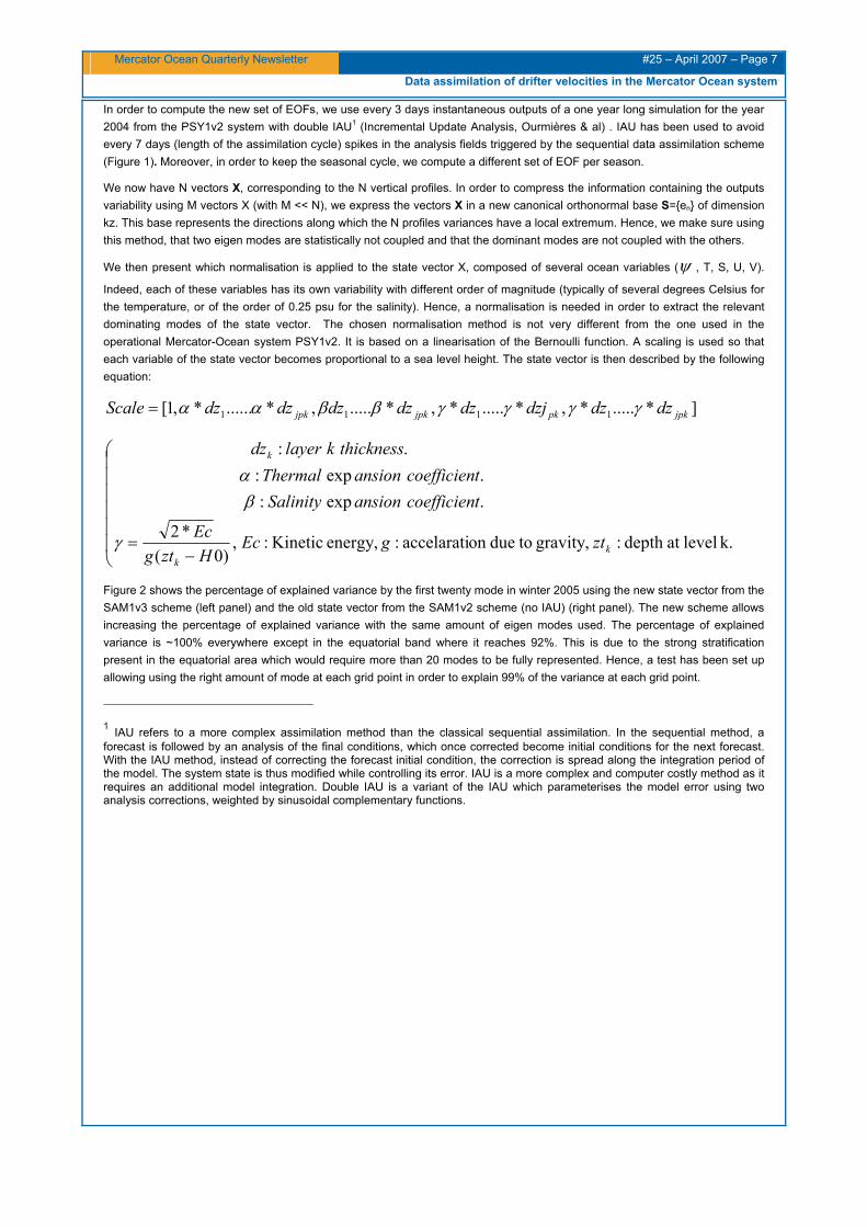
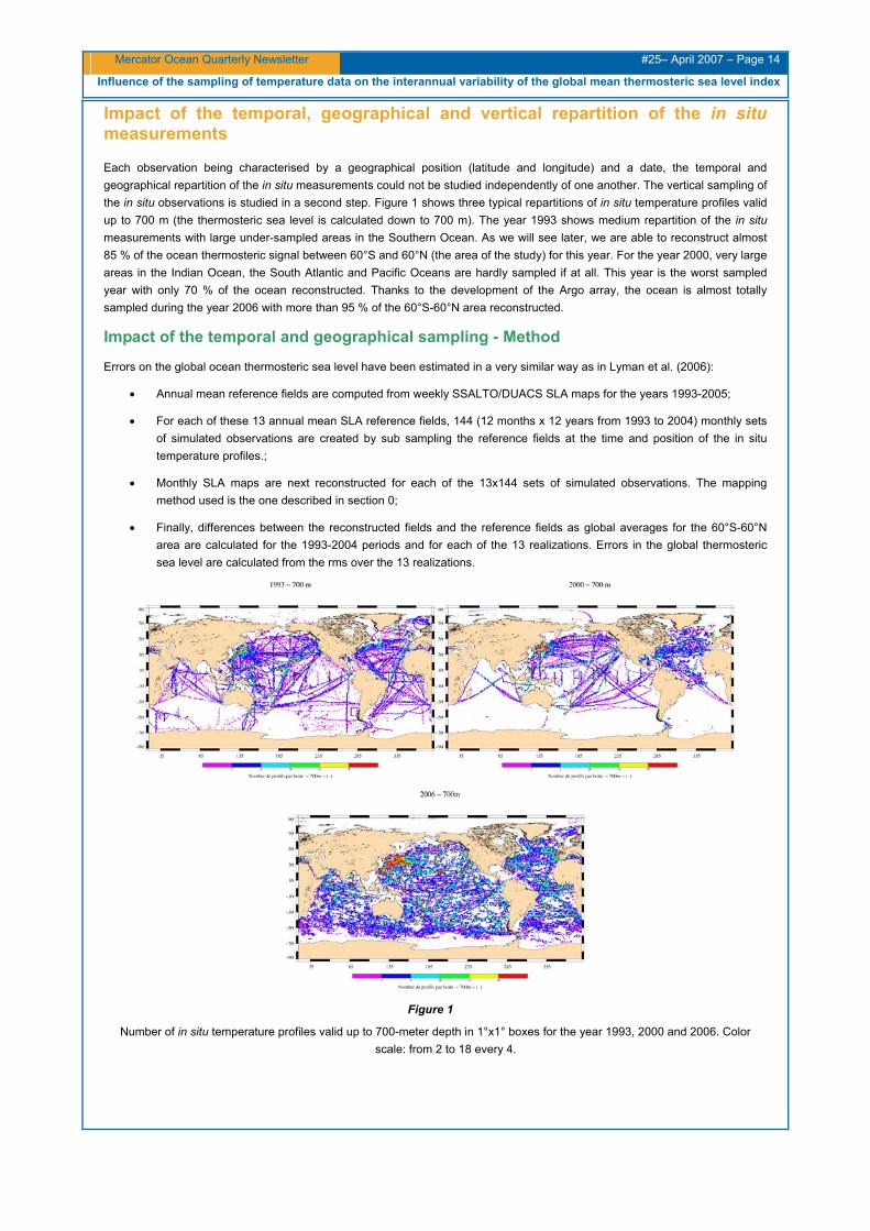
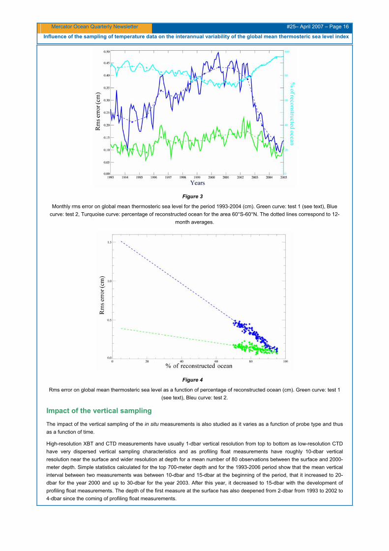
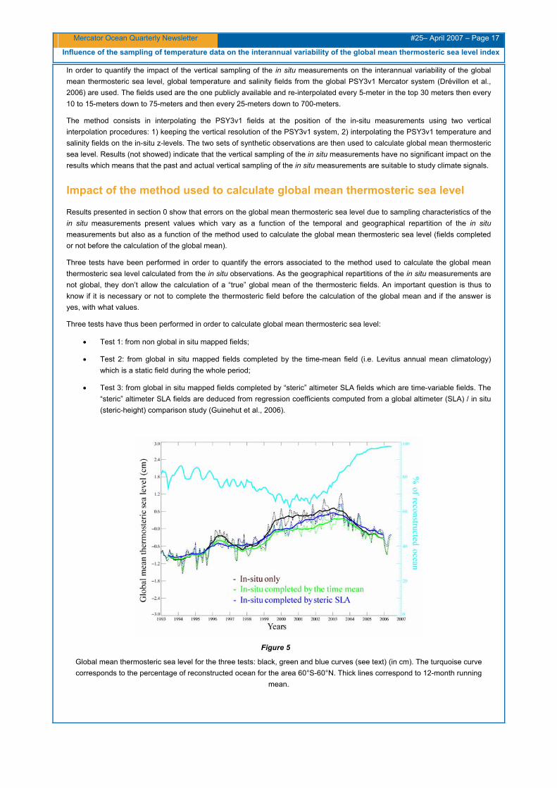
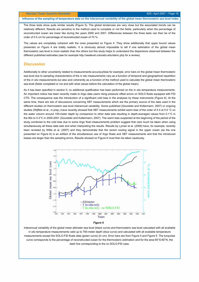
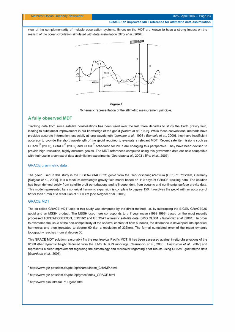
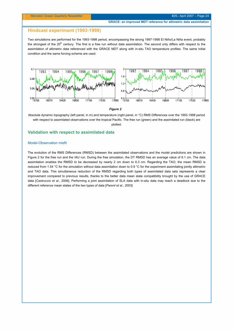
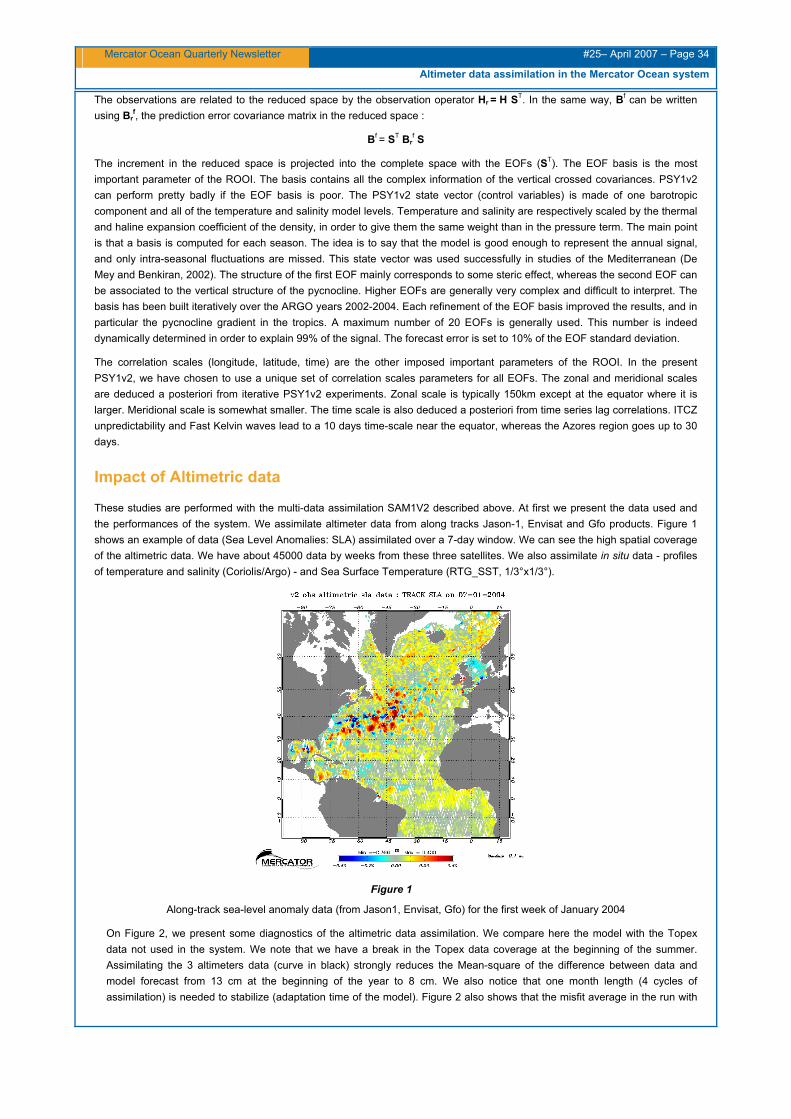