A SURVEY OF IRISH ELECTRONIC INDUSTRIES TOW ARDS

DEVELOPMENT OF A LOW COST M RP SYSTEM TO ENHANCE

THE EFFECTIVENESS OF THEIR INVENTORY CONTROL

PATRICIA GRACE (B .A ., B .A .I.)

M.Eng 1991

A SURVEY OF IRISH ELECTRONIC INDUSTRIES TOW ARDS

DEVELOPMENT OF A LOW COST M RP SYSTEM TO ENHANCE

THE EFFECTIVENESS OF THEIR INVENTORY CONTROL

BY

PATRICIA GRACE (B.A ., B .A .I.)

This thesis is submitted as the fulfilment of requirement

for the award of Master of Engineering (M.Eng)

by research to:

DUBLIN CITY UNIVERSITY

Sponsoring Establishment: EOLAS

September 1991

DECLARATION

I hereby declare that all the work prepared in this thesis was carried out by me at

Dublin City University during the period September 1989 to September 1991.

To the best o f my knowledge, the results presented in this thesis originated from the

present study except where references have been made. N o part o f this thesis has

been submitted for a degree at any other institution.

SIGNATURE OF CANDIDATE: _________ '

Patricia Grace.

CONTENTS PAGE

DECLARATION I

CONTENTS H

ABSTRACT V

ACKNOWLEDGEMENT VI

LIST OF MNEMONICS VII

CHAPTER 1: INTRODUCTION

1. Introduction 1

CHAPTER 2: LITERATURE SURVEY

2.1 Introduction 3

2.2 MRP and Lot Sizing Models 4

2.3 MRP n Lot S ize M odels 22

2.4 JIT Simulation M odels 31

CHAPTER 3: PRODUCTION SYSTEMS

3.1 Introduction 39

3.2 Idealized Structure o f a Manufacturing Organization 39

3.3 Examples o f Manufacturing Organization Structure 42

3.4 Types o f Production 44

3.5 Production Control 46

3.6 Push and Pull - 48

CHAPTER 4: INDUSTRIAL SURVEY

4.1 Introduction 54

4.2 Research Objectives 59

4.3 Research M ethod 60

4.4 Survey Results 61

4.5 D iscussion 93

4 .6 Conclusions 100

CONTENTS PAGE

CH APTERS: M ATERIAL REQUIREMENT PLANNING

5.1 Introduction 102

5.2 System Types 103

5.3 Processing Logic 106

5.4 MRP and Priority Planning 108

5.5 Operating Variables 108

5.6 Inputs to MRP 109

5.7 MRP and System Nervousness 114

CHAPTER 6: LOT SIZING AND MRP SYSTEMS

6.1 Introduction 115

6.2 Common Lot Sizing Procedures 116

6.3 MRP M odel 121

6.4 Solution Methods 130

6.5 The SCICONIC and MGG Packages 159

6.6 Results Section 165

CHAPTER 7: KANBAN

7.1 Types o f Kanban Card 182

7 .2 Rules Associated with Kanban Operation 183

7.3 Smoothing Production 187

7.5 Kanban M odels 188

CONTENTS PAGE

CHAPTER 8: A SIMULATION STUDY OF

KANBAN SYSTEM

8.1 SIM AN and Simulation 195

8.2 Simulation Objectives 198

8.3 Performance Measurements 198

8.4 Problem Specification 199

8.5 The Kanban M odel 200

8.6 Research Procedure 208

8.7 Discussion o f Results 209

8.8 D iscussion and Conclusions 268

CHAPTER 9: CONCLUSIONS

9.1 Survey o f Inventory Control Policies 272

9 .2 Lot Sizing Within MRP 273

9.3 Kanban Simulation 274

9.4 Recommendations For Further Work 275

REFERENCES

APPENDIX 1: MRP and JIT Survey Questionaire

APPENDIX 2: LINPROG 2 MRP Model Input and Results

APPENDIX 3A SCICONIC Model Input

APPENDIX 3B Matrix Generation Data File'

APPENDIX 3C Matrix File

APPENDIX 3D SCICONIC Results

APPENDIX 4A SIM AN Model File

APPENDIX 4B SIM AN Experimental File

APPENDIX 5: Nomenclature

APPENDIX 6: Tables o f Results: (6.18a, 6.18b, 6.19a, 6.19b)

ABSTRACT

This thesis is predom inantly concerned with the study o f inventory control practices

within the electronics industry in Ireland.

The study o f the inventory control system has been carried out under three main

interrelated sections:

Industrial Survey

D evelopm ent o f an M RP M odel

D evelopm ent o f a M aterial F low Simulation M odel

First, an industrial survey carried out to identify the com m on problem s and challanges

related to the electronics industry sector with respect to their inventory control

system s.

The results o f the industrial survey representing 44 com panies are presented. The

survey classifies the Irish Electronics industry sector in terms o f com pany size,

product structure and M RP levels.

Second, based on the industrial survey results a low cost M RP m odel has been

developed to enhance the effectiveness o f their inventory control system . The m odel

has been solved for a variety o f product structures using standard mathematical

programming packages. The results obtained are compared to those o f standard M RP

hot sizing techniques.

The third section involves the developm ent o f a material flow sim ulation m odel using

the SIM A N simulation package. The m odel is tested under a variety o f operating

conditions and perform ance statistics collected and analysed.

v

ACKNOWLEDGEMENT

I would like to express my appreciation to D r . M . A . E l B aradie for his guidance

and supervision during the course o f this project.

I would also like to thank M r. Jam es O ’K an e o f Staffordshire Polytechnic and D r .

M ich a e l O ’H eigearta igh o f Dublin City U niversity w ho introduced m e to S IM A N

and SC IC O N IC respectively.

Table (1.1): List of Mnemonics.L D C L ess D evelop ed C ou ntry .

N IC N ew ly In d u str ia liz in g C ountry.

M N C M u lti-N ation a l C om pany.

ID A In d u str ia l D evelop m en T A u thority .

C T T Irish E xp ort B oard

SF A D C OS h an n on F ree A irp ort D evelopm ent C om p an y .

A P IC S A m erican P rod u ction an d Inventory C on trol S ociety .

R & D R esearch and D evelop m en t.

M R P M ater ia l R eq u irem en t P lann ing.

M R P II M an u factu r in g R esource P lann ing .

W IP W ork in P rogress.

B O M B ill o f M ater ia l.

M P S M aster p rod u ction S chedu le.

IR F In ven tory R ecord F ile .

J IT J u st in T im e.

PT R P rocess T im e R atio .

V T T

CHAPTER 1

INTRODUCTION

In recent years western manufacturing circles have begun to place a great deal o f

em phasis on the reduction o f inventory at all stages within the manufacturing process.

Raw M aterial stocks, W ork-in-Progress, and the stocks o f F inished G oods have all

been earmarked for indepth analysis and reduction. The reason for this new

departure was primarily, the realization that a significant percentage o f working

capital was being needlessly tied up in these stocks. Capital investm ent costs w ere

also been ’sunk’ into the building o f large storage facilities to house these stocks.

This em phasis on inventory reduction sow ed the seeds for the developm ent o f tw o

manufacturing philosophies, which ideally offer two quite different solutions to the

sam e problem . - These two philosophies are termed M anufacturing Resource

Planning (M RP II), and Just-In-Time (JIT).

The main theme o f this thesis is inventory control, and with this in m ind, an integral

aspect o f each philosophy is exam ined in detail. The first section o f this thesis is

how ever, m ainly concerned with establishing the importance attributed to inventory

control techniques within Ireland today. A survey questionnaire was designed to

evaluate the extent to which M RP II and JIT have permeated the ranks o f the various

sections o f the electronics industry. Chapter 4 presents a brief review o f the effects

o f industrial policy on the internal m ake-up o f the industry, and with this in mind

presents a discussion o f survey results. Background information to this chapter may

be found in chapters 3, 5 and 6.

W ithin M RP II, a major area o f contention has been the ability o f M RP system s to

generate optim um requirements. Chapter 6 develops an alternate M RP model and

demonstrates it’s ability to solve the requirements problem for a variety o f product

structures. The m odels are solved using tw o standard -mathematical programming

packages, and the lim itations placed on the product structures by the capacity o f each

package, are investigated. F inally the developed m odels’ generated requirements are

compared against that generated by som e , o f the m ore w idely used L ot Sizing

procedures. Background to this chapter may be found in chapter 2 , 3 and 5.

The Just-In-Tim e philosophy controls and monitors material flow on the factory floor,

through the use o f a Kanban system . Chapter 7 , describes the Kanban system and

Chapter 8 develops a Kanban sim ulation m odel. The Kanban m odel is run under a

variety o f operating conditions and the m odel’s perform ance is evaluated, based not

only on inventory levels, but also on a number o f other perform ance characteristics.

Chapter 2 review s som e o f the background papers for this section.

CHAPTER 2 LITERATURE SURVEY

2.1 INTRODUCTION

The mathematical m odelling o f material requirement planning system s falls into two

distinct sections - nam ely scheduling and requirements generation. In this instance

how ever our interest lies only in requirements, and the generation o f optim um time

phased order requirements, through the use o f lot sizing techniques.

Typical system s in use today em ploy single-stage uncapacitated algorithm s, which are

applied sequentially to different levels, ignoring the concept o f inter-level

dependency. It is ironic to think that the backbone o f requirem ent planning system s,

- the ability to deal with inter-level dependency - is ultim ately ignored in the

preparation o f the final results and hence serves only to produce sub-optim al results.

Over the past two decades research into lot-sizing procedures has seen growth in two

directions. The first approach encom passes the work o f Zangw ill [1], L ove [2], and

others. It concentrates on the developm ent o f algorithms w hich yield optim al solutions

to the lot-sizing problem. T he second, is based upon the application o f single level

heuristics, but attempts are m ade to account for costs at each stage, and in so doing,

account for interdependencies betw een item s. N ew [3], Afentakis et al. [4] have both

worked in this area. Optim ization is the com m on factor in both approaches and it is

this which distinguishes present research from practise. The form er method how ever

seeks to produce optimal requirements, the latter to optim ize requirements produced.

The solution to producing optim al requirements lies in the use o f mathematical

programming techniques. A s objective funtions and constraint equations becom e more

com plex, and the problem size increases, processing tim e, and its reduction, becom es

increasingly important. W ith this in mind, new solution m ethods, exploiting certain

characteristics o f the constraint matrix are constantly being sought.

The question confronting many manufacturers today, especially those thinking o f

installing or upgrading an MRP system, is whether or not they are in fact being

cheated by being offered systems which do not produce optimum results.

The following review is not by any means an exhaustive account o f the development

o f lot sizing techniques and procedures, but a brief chronological review o f work

carried out on the topic, in order that:

a) The disparity between theoretical approaches to the lot sizing problem,

and the actual heuristics employed may be highlighted.

b) The potential that a good optimal approach to the lot sizing procedure

would offer a manufacturer, in terms o f saved investment might be

brought to the fore.

2.2 MRP LOTSIZING MODELS

2 .2 .1 The first lot sizing model was introduced by Wilson (see Browne et al. [5])

in 1915. It was called the Economic Order Quantity (EOQ). This model, and others,

such as the Period Order Quantity (POQ), and Part Period Balancing (PPB), which

were later developed from the Economic Order Quantity are still much in evidence

today. These methods seek a trade-off between set-up (or order) costs and carrying

costs, but all, are based upon three assumptions, namely

1. Cost structure is concave.

2. Demand for the item is assumed uniform and to occur

continuously over time.

3. All models are derived using differential calculus. (Browne et

al. [5])

The 1950’s however brought about a change in the fundamental approach to lot sizing

with the postulation that time could be divided into discrete time intervals, and that

demand for these periods could be forecast, or else was known. In order to determine

optimal requirement schedules, mathematical programming techniques were called

upon. One o f the first mathematical programming models was introduced by Wagner

Table (2.1):ZangwilI Model 1

M odel Summary Objective Function Constraint Equation

Zangwill (1969) (instantaneous

production).

m in:

E E (Cie p u * Hlt l i ti *1 t»i

+H'i t I l t )

(2.1)

If T N TE E ^ ’ E E ® »»>1 r=l i-l »-l

(2.2)

Single facility,multi­period,backlogging. Production,holding shortage costs. +IU = Dit‘,

(2.3)

Concave costs. Dynamic Algorithm.

= /ir=0;i= l

(2.4)

t=l..T

(2.5)

and Whitin in 1958, (see Z angw ill [1]). It w as based around the dynam ic

programming approach, and assumed identical costs in each period. T he m odel

referred only to a single product, produced on one facility but in m ultiple periods.

Dem and was not allowed to accumulate.

2.2.2 Zangwill [1], refers to the W agner-W hitin m odel [Table (2 .1 )] and

demonstrates how it can be represented in terms o f a network (the transhipment

variety). A concave cost structure is assum ed, w hich is show n to result in an optim al

flow which possesses certain peculiar properties. T hese properties are termed extrem e

flow s, (arborescences), and arise because, in single source networks w ith optim al

concave costs optimal flow s w ill be extrem e, and as such, nodes can have at m ost one

positive input. It is not feasible therefore to both place an order and receive goods

into stock within the same period. This relationship betw een concave costs and

extrem e flow s is very important, It the marginal costs o f holding an item from one

period to the next is greater than increasing the order size to be placed then the latter

is more feasible, - due to non-increasing marginal costs.

Zangwill [1] extends the W agner-W hitin m odel with a single facility and multi

periods to allow backlogging, (cumulating dem ands). [Table (2 .2 )] . This is done by

dividing up the inventory variable to represent both shortage and surplus amounts.

Instantaneous production is assum ed, although Zangw ill [1] says that all that is

required if lead times are to be accounted for is a sim ple redefinition o f the tim e

scale. The m odel is explained using network techniques and som e important

properties o f the optimal flow are developed. A dynam ic algorithm based on the

m odel is presented.

T he second part o f Zangw ill’s paper again deals with the single product m ulti-period

m odel but this tim e m ulti-facilities in series are assum ed. This m odel is also described

in terms o f network theory, and the properties o f the resultant extrem e flow s are

exam ined. A short three facility, three period exam ple is included to help explain the

algorithm.

Table (2.2): Zangwill Model 2

M odel Summary Objective Function Constraint Equation

Zangwill(1969).(InstantaneousProduction).

Mini

E ( c , J v - f l , /„) ¿=1

i= i . .r , i= i .

(2.7)

Single facility M ulti­period.Production and Holding costs.

/ M=/jr=0;i= l

P„ r ^ ; i = 1

(2.8)

Concave costs. Dynamic Algorithm.

iï r jv r

E E ' . - E E ® .¡=1 /=1 i=l f=l

(2.9)

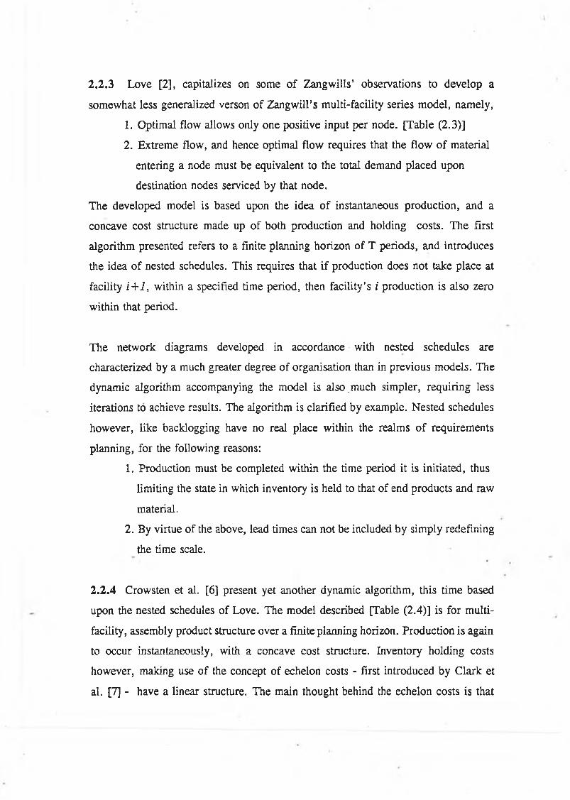
2.2.3 L ove [2], capitalizes on som e o f Z an gw ills’ observations to develop a

som ewhat less generalized verson o f Z angw ill’s m ulti-facility series m odel, nam ely,

1. Optimal flow allow s only one positive input per node. [Table (2 .3 )]

2 . Extrem e flow , and hence optimal flow requires that the flow o f material

entering a node must be equivalent to the total demand placed upon

destination nodes serviced by that node.

The developed m odel is based upon the idea o f instantaneous production, and a

concave cost structure made up o f both production and holding costs. T he first

algorithm presented refers to a finite planning horizon o f T periods, and introduces

the idea o f nested schedules. This requires that i f production does not take place at

facility i+1 , within a specified time period, then facility’s i production is also zero

within that period.

The network diagrams developed in accordance with nested schedules are

characterized by a much greater degree o f organisation than in previous m odels. The

dynamic algorithm accompanying the m odel is also .much sim pler, requiring less

iterations to achieve results. The algorithm is clarified by exam ple. N ested schedules

how ever, like backlogging have no real place within the realms o f requirements

planning, for the fo llow ing reasons:

1. Production must be completed within the tim e period it is initiated, thus

lim iting the state in which inventory is held to that o f end products and raw

material.

2 . By virtue o f the above, lead tim es can not be included by sim ply redefining

the tim e scale.

2.2.4 Crowsten et al. [6] present yet another dynamic algorithm, this tim e based

upon the nested schedules o f Love. The m odel described [Table (2 .4 )] is for m ulti­

facility, assem bly product structure over a finite planning horizon. Production is again

to occur instantaneously, with a concave cost structure. Inventory holding costs

how ever, making use o f the concept o f echelon costs - first introduced by Clark et

al. [7] - have a linear structure. The main thought behind the echelon costs is that

Table (2.3): Loye ModelM od el Sum m ary O b jective F u n ction C on stra in t E q u a tio n

L ove (1972) (Instantaneous P rod u ction ).

Min :

E (c„ v « , Ui=i*=1

(2 .10)

Pu-Pi.u +Iu i¿= i . j v ^ = i . .t .

(2 .11)

M u lti facility (series), M u lti period .P rod u ction ,H old in g costs. i= i..N j= i..T

(2 .12)

C oncave costs. D yn am ic A lgorithm . Optimal flow:

( 0

i=l . .Nj=l . .T.

(0)

k=ut z a z b z T

(2 .13)

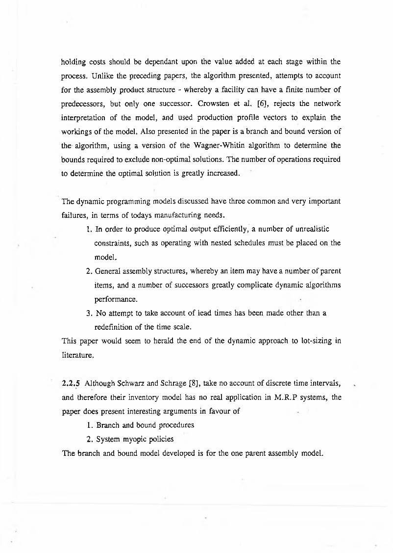
holding costs should be dependant upon the value added at each stage within the

process. U nlike the preceding papers, the algorithm presented, attempts to account

for the assem bly product structure - whereby a facility can have a finite number o f

predecessors, but only one successor. Crowsten et al. [6], rejects the network

interpretation o f the m odel, and used production profile vectors to explain the

w orkings o f the m odel. A lso presented in the paper is a branch and bound version o f

the algorithm , using a version o f the W agner-W hitin algorithm to determ ine the

bounds required to exclude non-optimal solutions. The number o f operations required

to determ ine the optimal solution is greatly increased.

The dynam ic programming models discussed have three com m on and very important

failures, in terms o f todays manufacturing needs.

1. In order to produce optimal output efficiently, a number o f unrealistic

constraints, such as operating with nested schedules must be placed on the

m odel.

2 . General assem bly structures, w hereby an item may have a number o f parent

item s, and a number o f successors greatly com plicate dynam ic algorithm s

performance.

3. N o attempt to take account o f lead tim es has been made other than a

redefinition o f the time scale.

This paper would seem to herald the end o f the dynam ic approach to lot-sizing in

literature.

2 .2 .5 Although Schwarz and Schräge [8], take no account o f discrete tim e intervals,

and therefore their inventory model has no real application in M .R .P system s, the

paper does present interesting arguments in favour o f

1. Branch and bound procedures

2 . System m yopic policies

The branch and bound model developed is for the one parent assem bly m odel.

Table (2.4): Crowsten et al. ModelM odel summary Objective Function Constraint Equation

Crowsten, W agner (1975)

(Instantaneous production)

min:

¿=1f=l

(2.14)

I = / +P -P •1it 1a-i r u¿=i..2V ^=i..r

(2.15)

M ulti facility (assembly), M ulti Period. Production,Inventory costs

0;

¿ = i . .^ = i . . r

(2.16)

Concave Production costs,Linear Holding Costs.

Optimal flow:

as before

(2.17)

The model developed [Table (2.5)] is based on the assumption that an optimal order

policy exists, whereby the ratio o f time lot size at stage i, to a successor stage is

integer. The inclusion o f set-up costs and echelon holding costs results in a convex

objective function and lower bounds to the problem may be generated using the

economic order quantity. A better bound may be found however by minimizing the

cost at each stage separately, and checking results to ensure that the lot size generated

at each stage i is less than that generated at an immediate predecessor stage. If this

is not the case then the costs at stage i must be modified, based upon the costs at an

immediate predessor stage, and the lot size regenerated.

If the lot size ratios at stage i and its immediate successor stages are integer, than no

branching takes place, otherwise the ratio is assigned an integer value and the relevant

costs are again modified, until all constraints satisfied.

The paper finally presents a discussion on system myopic policies, which are designed

to optimize a given objective function with respect to any two stages, ignoring

multistage interaction effects. The advantages o f myopic policies are listed as:

1. Easy to apply compared to branch and bound techniques.

2. Easy to understand.

3. Require less information than branch and bound.

4. Fast and very easy to compute.

5. Costs generated are very close to that of branch and bound.

2 .2 .6 Dorsey, Ratcliffe and Hodgson [9], present an efficient one pass algorithm for

the facilities in parallel problem - M facilities, any of which can fully process a

product-. The model formulation [Table (2.6)] differs from any previously

encountered. For each item, in each period a constant Wb is defined. This represents

the number of times product k must be scheduled in order to meet demand. Its

calculation is based on constant production rates, existing inventory, and demand.

Each individual item’s cost structure is used to develop an internal indexing term,

upon which the item’s scheduling priority per period is based. Therefore items which

incur the lowest holding cost would be scheduled first, thereby producing lowest

overall costs.

Table (2.5): Schwarz et al. ModelM o d e l S u m m a r y O b j e c t iv e F u n c t io n C o n s t r a in t E q u a t io n

S c h w a r z ,S c h r a g e (1 9 7 2 )( I n s ta n ta n e o u s )

Min:f f P H f i Ü Qi 2

(2 .4 6 )

Q r nQ *wi = l J V ;

n ^ ljn teger

( 2 .4 7 )

M u l t i f a c i l i t y (a s s e m b ly ) S in g le p r o d u c t .S e t - u p ,e c h e lo n h o ld in g

c o s t s .

hi=(l+p)h l+

2 P< E K

( 2 .4 8 )

C o n v e x c o s t . B r a n c h a n d b o u n d .

The approach adopted in this paper is of interest, both because of the model

formulation and also because it provides. insight into hierarchial requirements

planning. The approach adopted however cannot be expanded to develop efficient

algorithms for the solution of general assembly product structure.

2 .2 .7 The paper of Glover et al. [10], marks the emergence of generalised networks

onto the computer based production planning stage. The paper gives an informative

account of what a generalized network is, and its relationship to a linear program, -

similar to an L-P but having certain features which can be exploited in finding a more

efficient solution procedure The advantages of generalised networks over the more

general class of linear programs fall into two distinct areas.

1. Degree of solution efficiency.

2. Graphical interpretation.

The paper discusses how a coefficient matrix of certain linear programs can be

transformed via a set of linear transformations to a "node incident" matrix, with no

more than two elements per column.

A distinction is made between generalized networks and pure processing networks.

Shortest path, maximum flow, assignment, transportation, transhipment, all fall under

the pure processing class initially or by linear transformation, by virture of matrices

which consist of ones (not more than two per column) and zeros. The generalized

networks however allow integer constants other than one into the matrix.

The latter stage of the paper examines the efficiency of a computer code NETG, used

to solve generalized networks and identifies the following as being the critical factors

in determining solution speed.

1. Start up procedures

2. Pivot selection techniques

3. Degeneracy

4. Pivot tie breaking rules

5. Big M. valves

Table (2.6): Dorsey et al. ModelM o d e l S u m m a r y O b j e c t iv e F u n c t io n C o n s t r a in t E q u a t io n

D o r s e y e t a l .( 1 9 7 5 ) ( I n s ta n ta n e o u s p r o d u c t io n )

m in :tN^ ( 2 7 - - 2 i * l ) T ^ br=1 k -1

( 2 .4 9 )

k=1t=l..TJc=l..M

( 2 .5 0 )

S in g le C o m p o n e n t , m u lt i p r o d u c t , m u lt i fa c i l i t ie s ( p a r a l le l ) .f i x e d P r o d u c t io n a n d H o l ld in g c o s t s .

X ^ O ¡integer

( 2 .5 1 )

C o n v e x C o s t s .O n e p a s s A lg o r i t h m .

2.2.8 The algorithm presented by Dorsey et al. [9] becomes the basis of a multi­

item, series, multi-stage algorithm developed by Gabbay [11] [Table (2.14)]. The

underlying principle is that certain multi-stage systems can be treated as a sequence

of single stage problems. Restrictive assumptions regarding costs however must be

made. Production costs must decrease linearly with time, at each facility and for each

item, - ensuring production as late as possible -. Holding costs must increase with

each stage -ensuring that the item is kept in its cheapest form as long as possible.

The initial form of the model is similar to that of Zangwill [1], with the noticeable

exceptions that:

1. The objective function takes on a linear form.

2. A production constraint is included at each facility and in each period. But

for only one resource.

Before attempting to solve the model, Gabbay [11] eliminates the inventory variable

from the model and so reduces all equations to being expressed in production terms.

An aggregate production vector is introduced and defined recursively from stage i to

stage 1, (at each stage and in each period). Treating each stage as being independent,

the aggregate production at stage i+1 in period t becomes the demand in stage i,

period t. Feasibility conditions are reduced to that of a single stage system, namely

that aggregate cumulative capacity for each item, and stage over the planning horizon

must exceed or equal aggregate demand.

The paper also derives on interesting relationship between aggregate production and

capacity. Because cumulative production is being minimized, no inventory will enter

or leave a stage where total capacity is sufficient to satisfy demand.

The algorthim presented aggregates production and then disaggregates, item by item,

period by period. It is then used as a basis for the multistage case where instead of

disaggregating, modified planning horizons are introduced and the single stage

algorithm used to solve the problem over each period. Hierarchial or aggregate

planning has two main advantages:

I

Table (2.7): Gabbay Model.M o d e l S u m m a r y O b je c t iv e F u n c t io n C o n s t r a in t F u n c t io n

G a b b a y(1 9 7 9 )

(I n s ta n ta n e o u sP r o d u c t io n )

m in :M N T

E ( V » * «k-1(-1/=1

( 2 .5 2 )

t=l..T.

( 2 .5 3 )

M u lt i p r o d u c t ,m u lt i f a c i l i t y ( s e r ie s ) . P r o d u c t io n ,H o ld in g c o s t s

A a -1 ~J h t +A * =^ k i ’ k=l..m J=l..T.

( 2 .5 4 )

l i n e a r c o s ts M u lt i - p a s s A lg o r i t h m .

%

M

*=i

P kitJ^ Q ;i=l..Nj=l..TJc=l..M .

( 2 .5 5 )

1. It reduces complexity of problem.

2. Postpones any decision-making until more accurate data is available.

The assumptions made early in the model’s development in relation to costs together

with the assumption that production is proportional to item cost are however very

restrictive.

Aggregate planning techniques will probably have greater and more successful

applications at higher levels within the manufacturing control structure rather than

within the confines of material requirements generation.

2.2.9 Steinberg and Napier [12], monopolised on the work of Glover [11] and others

to present an inventory model which could be formulated as a generalised network.

The model is of the assembly variety, but can only accommodate single parents. The

objective function is obviously linear, incorporating production costs alone.

[Table (2.8)].

The model is comprehensibly formulated using a multi-source network interpretation,

both inventory and production variables are identically represented as charges (or

flows) incurred between component and manufacturing nodes respectively. Costs are

similarly represented as fixed charges between nodes. The indexing method used to

both construct and differentiate between terms within the model is complex and

confusing. Once formulated, Steinberg et al. [12] uses a mixed integer programming

package to obtain results for problems of up to four levels, three products and six

time periods. Processing time was found to be over seven minutes, for even small

problems.

Three important points in relation to solution times were made.

1. Very large problems can be decomposed into smaller product families,

where commonality exists within the family, but not without. Each problem

can then be solved independently.

Table (2.8): Steinberg et al. ModelM o d e l S u m m a r y O b j e c t iv e F u n c t io n C o n s t r a in t E q u a t io n

S te in b e r g ,N a p ie r (1 9 8 0 )

( I n s ta n ta n e o u s P r o d u c t io n )

m in :

EU* y

(2 .1 8 )

Network form'.

- £ /A

+ E

( 2 .1 9 )

M u lt i f a c i l i t y , (a s s e m b ly ) M u lt i p e r io d .H o ld in g ,p r o d u c t io n , p u r c h a s in g c o s t s .L in e a r C o s t s .L in e a r p r o g r a m m in g .

V . e J V

(2 .2 0 )

2. Computational effort might further be reduced by fmding a more efficient

method of determining upper and lower bounds on the various arcs.

3. A solution method which exploits the topological structure of the model

may prove very efficient.

2 . 2 . 1 0 The Steinberg and Napier [12] model, generated some controversy in lot-

sizing circles.The reasons for this were presented in a paper published by Thomas et

al. [13].

Firstly the S-N formulation (Steinberg and Napier), present results of small assembly

product structures, where quantities per parent items are represented as side

constraints. Thomas et al. [13] say that the presence of these side constraints make

it impossible to solve the model using existing network codes.

Secondly, as seen in the S-N formulation, the network consists of

1. Purchase, component, assembly nodes.

2. Purchase, inventory, manufacturing, fixed charge arcs.

3. Side constraints to maintain proportionality of requirements.

Each node is labelled according to product level and period, and therefore requires

six subscripts to identify each node. Thomas [13] points out that this is too

cumbersome and confusing.

Thomas [13] presents a final point relating to the formulation of side constraints

within the S-N model, and presents a more efficient method which reduces the

number of constraints.

An alternate model formulation is presented [Table (2.9)] in which holding costs and

set-up costs are included in the objective function and the major constraint is the

standard form of the material flow equation.

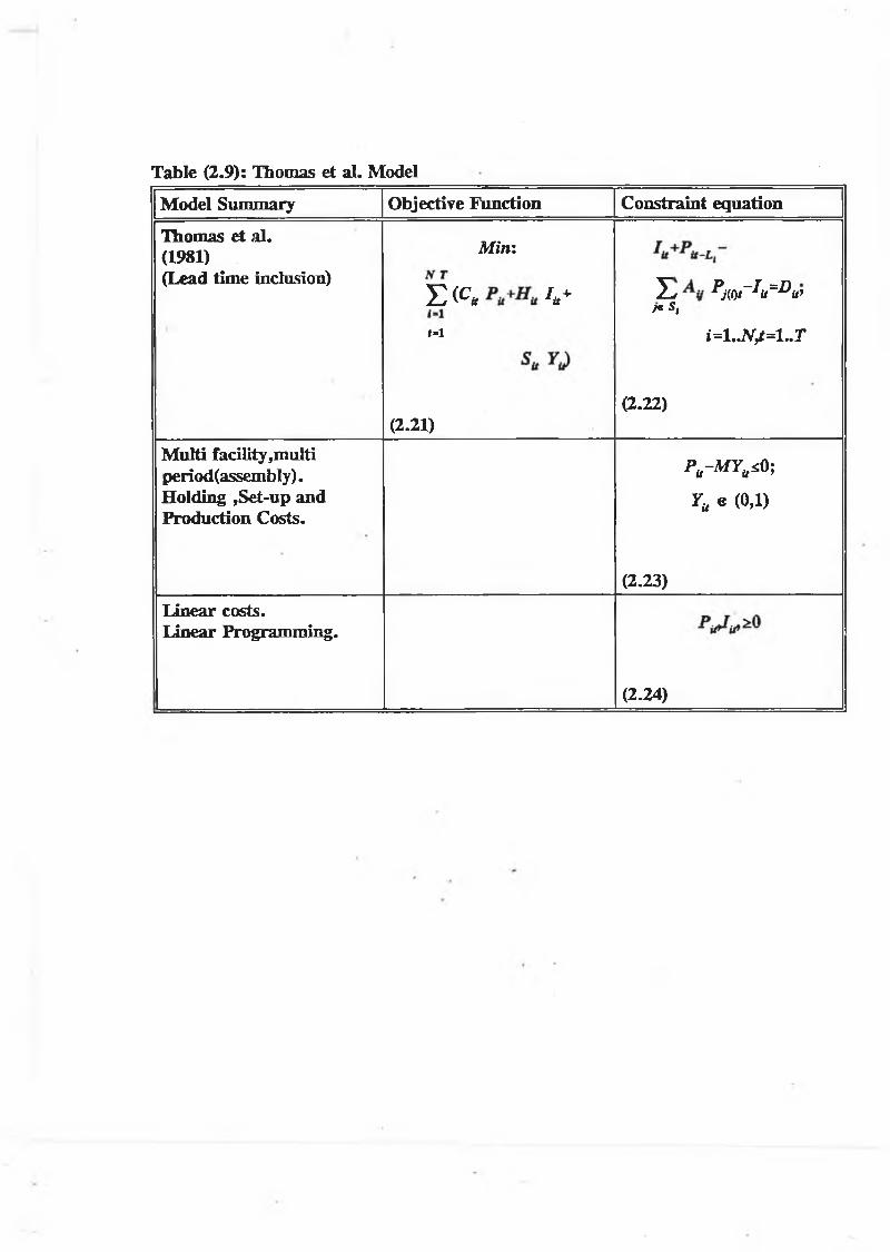
Table (2.9): Thomas et al. Model

M o d e l S u m m a r y O b j e c t iv e F u n c t io n C o n s t r a in t e q u a t io n

T h o m a s e t a l .(1 9 8 1 )(L e a d t im e in c lu s io n )

Mini

E ( C , V

f-1

(2 .2 1 )

X / PM r Tu=I)u’/e 5,

i = i . j v ^ = i . . r

( 2 .2 2 )

M u l t i f a c i l i t y ,m u l t i p e r io d ( a s s e m b ly ) . H o ld in g , S e t - u p a n d P r o d u c t io n C o s t s .

Pu-M Y uiO;

Yu e (0 ,1 )

( 2 .2 3 )

L in e a r c o s t s .L in e a r P r o g r a m m in g .

( 2 .2 4 )

2 .2 .1 1 Blackburn and Millen [14] present results from the pursuit of research along

an alternate path to the optimum solution, - the sequential application of a single stage

algorithm with a set of modified costs in an attempt to account for interdependencies

between items. For explanations of the various single stage algorithms see Chap. 6.

The work of Blackburn and Millen owes much to that of Schwarz and Schräge [8],

and their continuous time model.

The model seeks to minimize holding costs and set-up costs. Production costs are

assumed zero. The concept of echelon stock at stage is incorporated into the model.

The objective function is described in terms of set-up and echelon costs, together with

an order interval variable r, (specified in time periods) which established the rate of

placement of orders. The lot-sizing problem therefore reduces to finding a set of

values which minimises the average cost period. These values are determined

iteratively down through the product structure by evaluating ku (ratio of ^ stage i to

nt at parent stage. The k{ values represent the number of orders from parent stages

which are combined into a single order at stage i. These values once determined can

then be used to minimize costs. The paper presents five methods of determining these

values.

The empirical work described in the paper centres around serial (two and three stage)

and assembly (five stage) systems. In both cases varying combinations of single level

heuristics, with and without modified costs were used in order that the performance

of the adjusted cost methods could be ascertained. In each case, the adjusted cost

methods retained a computational efficiency comparable to single stage lot-sizing

algorithms.

2 .2 .1 2 The previous model formulation, Blackburn and Millen [14], is similar to that

of Akentakis et al. [Table (2.10)]. Not only does the model seek to minimise set-up

and holding costs but also included is the concept of echelon holding stock. The

material flow constraint equations are rearranged in terms of echelon stock. Because

of this demand terms generated internally (at intermediate levels), must be expressed

in terms of echelon stock also.

Table (2.10): Akentakis et al. ModelModel Summary Objective Function Constraint Equation

Akentakis et al. (1985) (variable lead time) min:

NT

E (s. Vi-K -l

H i Eh

(237)

e L + p u- e I=

A VDM ‘>i= l..N j= l..T

(238)

Single Product, multi penod^muld facility (assembly).Set-up,Echelon Holding costs.

i=l..nJ=l..T.

(239)Linear costs. Branch and Bound. -E l*0;t=l..T

PuiY u;l= l..N j= l..TY ^ l h P ^ O

(2.40)

Akentakis et al. [4] have not presented an optimal solution to the problem, and

because of this a comparison can not be made between this model’s performance and

that of Blackburn and Millen [14]. Some properties of the optimal solution are

presented. The first of these is similar to the nested schedules idea of Love [2] and

Crowsten et al. [6] in that if, facility i+1 produces in period t, then the facility i must

also have produced. The second property, follows from the first, and states that if

production at any facility i, period t is optimal, then an optimal production schedule

exists at facilities i+1 to final assembly (straight path). The third property also makes

use of Love’s [2] result for an optimal solution which says that there exists an optimal

solution in which each node can have only one positive input. This implies that the

search for optimality is limited to the subset of all feasible solutions. This subset

consists of the set of all plans in which item i appears in period t, only when the

echelon stock of i, at the end of the previous period is zero. The final property relates

to branch and bound solutions and the use of Lagrangian relaxation to tighten the

bounds. It states that shortest route algorithms can be used to solve the problem

following treatment using Lagrangian relaxation.

Akentakis [4], shows how this new treated function may become the bound (lower)

for the problem, and shows how the bounds themselves can be optimized. The upper

bounds are generated using a single level heuristic. The mathematics of obtaining

bounds are fairly complex and a background in Lagrangian would be advantageous.

The final section of the paper deals with the performance of the branch and bound

algorithm itself, and the testing of four different assembly systems each with a

varying number of nodes and levels. The algorithm performed well in all cases and

computing time deemed reasonable. Large scale problems however were stated to be

beyond the scope of the algorithm and the usual constraint of only one parent per item

applied.

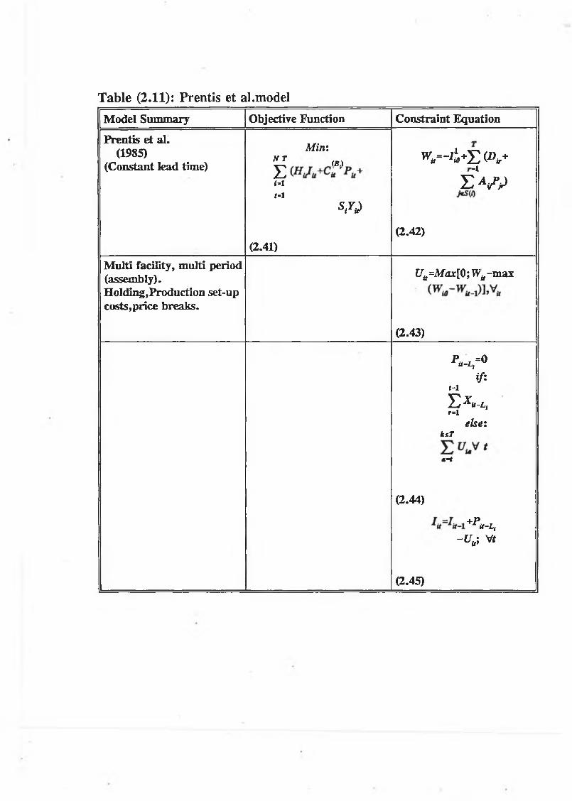
Table (2.11): Prentis et al.modelM o d e l S u m m a r y O b je c t iv e F u n c t io n C o n s t r a in t E q u a t io n

P r e n t is e t a l .(1 9 8 5 )

( C o n s t a n t le a d t im e )

Min:

NT a nE¿-1M

w

(2 .4 1 )

w.-ii+Eu»^

e V p

( 2 .4 2 )

M u l t i f a c i l i t y , m u lt i p e r io d (a s s e m b ly ) .H o ld in g ,P r o d u c t io n s e t -u p c o s t s ,p r ic e b r e a k s .

Uu=Max[ 0 ; W ^ -m a x

(2 .4 3 )

p«v°ifi

t-1

E vr= l

else'.ks.T

m-t

( 2 .4 4 )

+Pu-L, ~UU; V i

(2 .4 5 )

2.3 MRP n LOT SIZE MODELS2.3.1 Zahorik et al. [15], formulates a multi-facility, multi-period, multi-product

model for the parallel series product structure. Each product however must go though

a similar sequence of production steps. [Table (2.11)].

The model is formulated very comprehensibly with the objective function consisting

of both production and holding costs. The constraint equations include the usual

material balance constraints but added to these are a number of capacity constraints.

The first of these limits the total amount of production at any stage. A similar

restriction is also placed on inventory at any stage. These two constraints are termed

bundle constraints. (Constraints on total thruput at any stage). Upper bounds are also

placed on individual production and inventory variables at each level.

In order to solve the presented model, the bundle constraints must be limited to occur

in the following three forms:

1. On inventory at any stage.

2. Total production at the final stage.

3. Total production and inventory at any stage.

Generally speaking, bundle constraints cannot be modelled as networks however the

paper reveals network properties of bundle constraints as long as the planning horizon

is less than or equal to three periods: This is later used as the basis of a rolling

algorithm, which is presented in the paper.

The paper constructs the constraint matrix for bundle constraints applied at the

various allowed levels. The node-incident matrix obtained after the application of a

number of linear transformations is also presented. Two cases are said to arise

however, in which the application of bundle constraints in the three period case, will

not result in a network structure.

1. If there exists bundle constraints of either type at more than one level.

2. if production constraints are not at the same level as inventory constraints.

Table (2.12): Billington et al. ModelM o d e l s u m m a r y O b j e c t iv e F u n c t io n C o n s t r a in t E q u a t io n

B i l l in g t o n e t a l . (1 9 8 4 ) (V a r ia b le le a d t im e )

m in :

E ( » . V C , r„ )«=1t- 1

D T

+ E ( C O ^ C U ^ U JJ -l1=1

(2 .2 9 )

h - x + n f u - L r 1 * -N- 1

E AiP w =Du’/OM

(2 .3 0 )

S in g le p r o d u c t ,M u lt i F a c i l i t y (a s s e m b ly ) , M u lt i P e r io d .H o ld in g ,p r o d u c t io n ,s e t u p ,o v e r t im e ,u n d e r t im e c o s t s .

E

d=l..DJ=l..T.

( 2 .3 1 )

l i n e a r C o s t s , l i n e a r p r o g r a m m in g .

P a - ^ 0 ;

i = i . .A 7 = i . . r9 v.

(2 .3 2 )

The rolling algorithm presented in the latter stages of the paper becomes exceedingly

complex as the number of levels within the product structure increases. An increase

in the number of bundle constraints combined with a similar increase in the number

of levels often results in a solution which has little or no advantage over traditional

linear programming solutions. For the multi-level problem therefore, Zahorik et al.

[15], suggests one or two period rolling in order that an opportunity for cost

reduction can be found.

The empirical work outlined in the paper deals with the computational efficiency of

two linear programming packages, LINDO and MRSX (produced by DEC and IBM

respectively), compared to that of the rolling algorithm. Results presented would seem

to point to the superiority of the rolling algorithm.

This paper is unique among those reviewed so far in that it transcends the bounds of

simple requirements planning, by attempting to incorporate capacity constraints and

in so doing, develop a finite loading model.

2.3.2 Billington et al. [16], provides a very general approach to capacity constrained

systems [Table (2.8)]. The model developed is for the multi-period, multi-facility, one

parent assembly product structure. The final form of the model incorporates set-up

costs, holding costs, and under-time, overtime costs within the objective function. The

paper tackles the problem of lead-time and lot-size interactions. Lead times are said

to be made up of the following:

1. Set-up times

2. Production times

3. Wait time

4. Removal/Transport time

Capacity constraints placed upon facilities will ultimately affect the above, and

because of this it is assumed that lead times as well as lot-sizes are variable. The

problem then reduces to the simultaneous determination of -

1. Lot-sizes.

Table (2.13): Ho et al. ModelM o d e l S u m m a r y O b je c t iv e F u n c t io n C o n s t r a in t E q u a t io n

H o j M e K e n n y

(1 9 8 8 )( v a r ia b le le a d t im e s )

MiniNR,E ( H J u + WM(=1

( 2 3 3 )

h - r h + p « -AyPMt+L/.o=Diti = l . .A r = l .J ? r

( 2 .3 4 )

S in g le p r o d u c t , m u lt i p e r io d , m u lt i f a c i l i t y ( a s s e m b ly ) . P r o d u c t io n ,H o ld in g c o s t s .

Pa=04=l>Nrt= lX i^10 JiR.{ -I'-MPu> 0 ^ ^ 0 , 1 =1..NJ=1. J ? r

( 2 .3 5 )

L in e a r C o s t s l i n e a r P r o g r a m m in g .

•{Capacitated form)

E £ v . £ t / * ;¿=ld=\..D j=l..T .

( 2 .3 6 )

2. Lead times.

3. Capacity utilization.

The problem is formulated as an integer-linear program. Billington et al. [16] states

that the model can be solved using leontif substitution systems when only the material

balance constraints are applied. As yet however, no solution has been found for the

global problem. Both

1. Decomposition

2. Lagrangian relaxation

have been suggested as possible solution techniques.

As with all MRP models, demand (in discrete time periods) initiates production.

Changes in capacity however due to breakdowns, lack of personnel etc. are not

provided against within the model. Billington [16] suggests three methods which'

might provide against any unforseen changes.

1. The objective function could be modified to minimise a discounted sum of

slack production

2. Reduce the RHS (right-hand side) of capacity constraints to below its

known limit, thus keeping some in reserve.

3. Build buffer inventory into the master production schedule.

The latter half of the paper deals with the possible reduction of the ILP. The crux of

this procedure lies in the definition of a constrained facility.

"A facility upon which the time limit is likely to be a binding constraint, often

enough and for a long enough duration to cause a scheduling difficulty".

Unconstrained facilities would be scheduled for in a lot-for-lot fashion', once the

constrained facility is determined. The following two rules must be adhered to, in

order that the compression of the ILP is successful.

1. Variables relating to all items with significant set-up costs,

and/or items produced on a constrained facility must remain.

2. Variables belonging to items that

a) share a common item

b) eventually form part of type 1 items must also remain.

Table (2.1/ ): Zahorik et al. ModelM o d e l S u m m a r y O b j e c t iv e F u n c t io n C o n s t r a in t E q u a t io n s

Z a h o r ik c t a l .(1984)

(C o n s t le a d T im e .)

m in :M2VT£ <c * , j v*=i(= 1

i=i

•

(2.25)

Conservation

of Flow:A Ek=bk;k=l.Jtf

(2.26)

M u lt i p r o d u c t m u lt i f a c i l i t y (se r ie s ) m u lt i p e r io d .P r o d u c t io n ,h o ld in g c o s t s . -

E ' a  v „;Jt-1

i

(2.27)l i n e a r C o s ts , l i n e a r p r o g r a m m in g . ® kü^kU’

(2.28)

The rationale behind these two rules is that items produced on constrained facilities

will have lead times which depend upon the capacity available. Items with large set­

up costs must also remain to allow batching.

The compression itself is done in two phases. Firstly any reference to items which

will be subsequently used by Lot-For-Lot items all the way to End-Item level are

eliminated. The second phase elimanates any Lot-For-Lot items which don’t share

common inputs. The resultant product structure is substantially reduced. By isolating

lead times and lot-sizes, as being two of the major contributors to a manufacturing

system’s overall performance, the model secures the foundation for a good MRP

model. Lead times are not, as generally assumed, instantaneous, but may be thought

of as function of work-in-progress, which in turn is dependent on time accumulated

during processing.

2 .2 .3 Ho and McKenney [17], present a short paper, the general theme of which is

that although the presented models are not network linear programs, they possess an

interesting network property, namely that they can be triangularized by successive

applications of linear transformations. The models presented, introduce both

production and holding costs, and the constraint matrix is made up of material flow

equations in the usual fashion. The equations however are slightly modified by the

introduction of dynamic or varying planning horizons for the various facilities. [Table

(2.13)]. Production and inventory variables for a particular facility are constrained to

occur within the planning horizon span at that facility. The calculation of this horizon

is based on the planning horizon and lead time at a parent facility. •

Ho et al [17] suggest that triangularity property of the constraint matrix means that

the operations of the simplex method would ultimately be reduced to a set of back

substitutions and hence greatly reduce processing time. He also suggests formulating

the problem as a network with side constraints would result in an optimal solution.

The second model presented, is similar to the first with the exception of a further

constraint which limits the total capacity available at each facility. This model is

referred to as the multi-product finite loading model. Ho et al [17] suggests Dantzig-

Wolfe Decomposition as being a possible solution procedure, once advantage has been

taken of the triangular nature of the basis.

2 . 2 . 4 Prentis and Khumwala [18], present a multi-period, multi-facility, general

assembly model [Table (2.14)]. The objective function includes both production,

carrying and set-up costs, and has the capability to handle cost breaks, in both

production and purchasing. It is said to be piecewise, both concave and convex, (non

convex) which excludes any linear programming from directly solving the problem.

The model is the most comprehensive to be found in literature, and is solved using

a complex branch and bound technique. The technique is explained in the paper and

an example problem solved.

Prentis compares computational results, using his branch and bound method, with a

number of other well known lot-sizing techniques, over a variety of demand patterns.

It is found that in all cases the branch and bound technique performs better than any

of the other methods.

2.4 TIT SIMULATION MODELS

2 .4 1 I n t r o d u c t io n

Unlike the techniques of analytical mathematics which have been used to solve a

variety of problems for hundreds of years, simulation is a relatively new method of

problem solving made available by huge advances in the processing capability of

computers. In recent years, simulation is being used more and more in the

manufacturing field to investigate various systems’ performance under a variety of

operating conditions.

Within manufacturing, simulation techniques would appear to have found a particular

application in the relatively new areas of JIT production and flexible manufacturing,

as a means of explanation as well as experimentation.

This section of the survey provided a brief review of some papers which develop

simulation models, with application in the Just-In-Time environment either as a means

of experimentation or as learning tool for others.

2.4.1 Huang et al [19], present an interesting paper, investigating the effects of

variances on system performance using the following parameters.

1. Kanban cards at each stage.

2. Processing times at various stages.

3. Demand rates.

4. Combinations of the above.

The paper initially provides a very comprehensive explanation of the operation of a

two-card Kanban model, and its translation into a Q-GERT simulation model. The

actual model simulated is a variation of a 3-line, 4-stage general assembly model,

described in Chapter 8.

The first experiment conducted, investigates the effects of various processing time

distributions (all work-stations having the same processing time) for systems with both

1 and 2 Kanban cards. Performance parameters include overtime, production rate,

and input and output buffer inventory levels at final assembly. The second experiment

examines the effect of bottleneck located at various positions along as assembly line,

and the third experiment examines the effect of demand distribution variablity. The

interactive effects o f demand and processing time variability are also investigated. In

each case, performace parameters are as described above.

The main conclusions are as follows:-

In order to effect a transfer to JIT production, large increases in overtime must be

expected, in an effort to reduce process time variation. An overtime ban would only

serve to increase work-in-progress and an inability to meet the demand schedule:

Bottle-necks can not be tolerated within a JIT system, because their effects can not

be counteracted by system parameters such as the number of Kanban cards: JIT

production can not be operated effectively while there is a degree of variability at

demand level.

2 .4 .2 Ebrahimpour et al [20], take a slightly more indepth look at the effect of

Kanban card usage on work-in-progress inventory. The model presented is that of a

two-stage production line. The model is coded using the DYNAMO simulation

language.

Two types of demand patterns are under investigation, that of cyclical demand, and

constant growth demand. Simulation runs are carried under both these conditions,

firstly to quantify the degree to which production can keep up with sales, and

secondly to investigate the rate at which the Kanban cards can be reduced, without

adversely affecting production.

The main conclusion of the paper is that under both sets of operation conditions, the

reduction of the Kanban cards operation within the system does not cause production

to lag behind sales, but does cause a significant reduction in work-in-progress

inventory. It was also found however that there is a point beyond which further

reduction of the cards does affect production.

2.4.3 Schroer et al [21], use a Kanban production model to investigate the operation

ot the SIMAN simulation package. The paper appears to place greater emphasis on

both the performance of SIMAN and the development of the simulation model for an

assembly line consisting of two assembly cells that on the actual model performance.

The paper concentrates on the levels of work-in-progress at various points withing the

system, both one and two kanban card operation were investigated.

The paper is of note mainly for its use of the Siman language. No conclusions are

made on the basis of results presented.

2.4.4 Sarker et al [22], use the SIMAN simulation language to investigate the effect

of a number of umbalancing methods on a number of system performance parameters,

- queue lengths, machine utilizations, waiting time, cycle times, and finally

production rates. The actual simulation model consisted of a six-stage assembly

process.

Four unbalancing methods were analysed. The first, referred to as the see-saw effect,

involved isolating three stations, and simultaneously increasing and decreasing the

processing times of the first and third stations respectively. The second and third

methods involved the creation of a processing time bowl over three and five stations,

(i.e. the middle stations have lower-concave and higher-convex processing times).

The effect of a change in only one stage, in one line is also investigated.

The main objective of the paper is to evaluate the operation of the various

imbalancing methods and in so doing, afford production managers useful insight into

the implication at the various stages so that they can adjust system parameters

accordingly. The various conclusion pertaining to each and every system

configuration are too numerous to mention here, however the paper does prove that

a balanced configuration ensures optimum system performance.

The paper concludes with a similar observation to that o f Huang et al [19], - that

Western manufacturers cannot immediately transfer to JIT production without

evaluating the various requirements of the new system and making the appropriate

modifications. Simulation techniques are very useful in this respect.

2 .4 .5 The paper of Browne et al [23], presents quite a complex simulation model,

which has application in the testing of control mechanisms for flexible assembly

systems.

The actual simulation model which is coded in SLAM II consists of a 5 station

assembly line, each station having a maximum of 5 feeder stations, although this

number may be varied. A total of our individual products may be produced on the

mode. Two different types of sequencing methods are available: an MRP type

sequence, and a Kanban sequence, the object of which is to develop uniform work

loads on the line. The model allows the modeller to choose from a variety system of

the system performance parameters, such as processing times, etc. Various limitations

and assumptions are listed in the paper.

Unlike the previous papers reviewed, this model is more complex, being produced

and developed not only for use bt the developers themselves, but also for other

experimentors who are interested in simulation results but not in actual model

building. The last section of the paper discusses an experiment which investigates the

effect of batching and set-up times on JIT production.

The main conclusion from the experimental section is that failure to reduce the set-up

time, while reducing the batch size causes reduction in the production rate of the

system.

2.2.6 The paper of Villeda et al [24] is similar to that of Sarkar et al [22], in that

the area of investigation is unbalanced production lines. There exists two notable

differences however. Firstly, Villeda [24], is interested in both mean and standard

deviation variances, and the range of variation is much smaller than that of Sarkar et

al [22]. Secondly, each of the system configuration investigated may be referred to

as bowl shaped. The simulated model consists of a three line assembly system, with

three work station at each line.

The first experiment isolates the unbalancing method with the greates potential to

increase the systems performance. All the experiments are then carried out with

reference to this method. Variation in the standard deviation of the processing times

are investigated for systems operating with one and two card Kanbans. Performance

measures include production rate, mean utilizations, mean wait time at final assembly

etc. The third set-of experiments investigates the introduction of variability at final

assembly. Again the same performance measures are used.

The paper of Sarkar et al [22], demonstrates that when the unbalanced range is large,

and the increments in processing times are also compariably high, balanced system

will always outperform an unbalanced one. Velleda et al. [24] however, isolated a

small unbalance range, where unbalanced systems outperform balanced ones for all

the umbalancing configurations used.

The paper of Sarker et al [22], demonstrates that when the unbalanced range is large

and the increments in processing times are also compariably high, balanced systems

will always outperform an unbalanced one. Villeda et al. [24] however, isolates a

small unbalanced range, where unbalanced systems outperform balanced ones for all

the unbalancing configurations used.

CHAPTER 3 PRODUCTION SYSTEMS

3.1 INTRODUCTIONIn the words of Goldratt and Cox [25] the primary aim of any manufacturing concern

is to make money. Secondary aims, which complement this include:

1. To satisfy customer orders on time, and with least costs.

2. To maintain/obtain a good market share.

In order to satisfy these objectives, a manufacturing firm, requires a formal structure

within which it can seek to operate successfully. Many books, have been written,

attempting to describe this formal structure, and although, the basic principles and

concepts, never change, literature shows that the actual description of this structure,

is subject to the individual’s interpretation.

3.2 IDEALIZED STRUCTURE OF MANUFACTURING

ORGANIZATIONAn idealized interpretation of this structure is shown Fig (3.1a). This figure shows

the overall structure within which two subsystems operate, namely:

1. The manufacturing technology system.

2. The manufacturing management system.

It is within the manufacturing technology system, that, the origins of the whole

structure lie, with the design function. Once product designs have been decided

upon, the production planning function is called upon, to create the routing system

necessary to ensure the correct manufacture of the product according to the design

specifications. Once this route has been decided upon, the relevant data is then given

to the costing function, within the manufacturing management system, to evaluate

production costs for the product, on the basis of routing, times, and process times etc.

imparted by the production planners. Production costs, are traditionally derived from

a division of costs, into three categories [26,27],

1. Direct Labour Costs.

2. Direct Material Costs.

Idealized Structure of a Manufacturing Organization. Fig.(3.1a)

3. Overhead Costs,

although, advances in such areas as automation, inventory control, are rendering this

method of costing a "Dinosaur". Direct labour used to account for 50% of prime

costs (Direct Labour -1- Direct Material), now it may account for as low as 2-3%,

with the result that time spent, on trying to reduce, labour costs, would be much

better spent, focusing on inventory or overhead reduction. A new method, of costing

has developed, termed throughout accounting, based on two concepts [28].

1. A factory is not a collection of individual resources, but an integrated

system of processes and machines, and as such the term, -total factory

cost, -refers to all fixed costs originating in the factory.

2. Products on their own are neither profitable or unprofitable, it is the

rate at which the product contributes money that determines relative

product profitability.

Once costs have been decided upon, the production control function, in the

manufacturing management system, is required to:

"Plan direct and control, material supply and processing activities, of

an enterprise, so that specific products, are produced, by specified

methods to meet an approved sales program, these activities being

carried out in such a manner that the labour, plant, capital available,

are used to the best advantage".

Which is essentially equivalent to saying of the production control function, - that it

guides material flow, through the material flow system, as created by production

planning - This material flow system, consists of the route a particular product takes

as it traverses the manufacturing system.

As material, flows through the manufacturing system, monitored closely by

production control, stock, in terms of Work-In-Progress (WIP) is generated. The

inventory control function, is required to maintain, this type of stock, and both raw

materials, and finished products at a required level. Inventory control was often

thought to be secondary to production control, [29] in that, production control is

administered, with the aim of keeping inventory at an optimum level. The realization

of the enormous benefits of a reduced inventory level has afforded it a higher status

than previously.

Quality control is somewhat, of a misnomer within the manufacturing structure,

fitting neither into the manufacturing management system, or into the manufacturing

technology system, but at the same time being part of both. With the emergence of

the Just-In-Time and Total Quality Control, manufacturing philosophies, a certain

shift in emphasis in the role of quality control has also taken place, with the quality

control procedures being built into the manufacturing process as much as possible,

and making quality managers, responsible, only to the top level in the hierarchal

management structure.

" The final function of the manufacturing management system is despatch, - the actual

removal of goods from the factory and transportation to the customer.

3.3 EXAMPLES OF MANUFACTURING ORGANIZATION

STRUCTUREAs mentioned previously a wide range of literature is available, describing this formal

structure. Burbridge [29], refers to this formal structure as a productive system,

within eight management functions operate, namely.

1. Financial 4. Personnel 7. Design

2. Marketing 5. Purchasing 8. Secretarial

3. P. Planning 6. P. Control

With this structure, production planning and design, and both the production control

and financial functions are closely related.

Wilde [6] speaks of operating systems:

"An operating system, is a configuration of resources combined for the

function of manufacture, transport, supply or service".

Operations management therefore, is concerned with the design and operation of the

system. Operations management is divided into two main areas, design and planning,

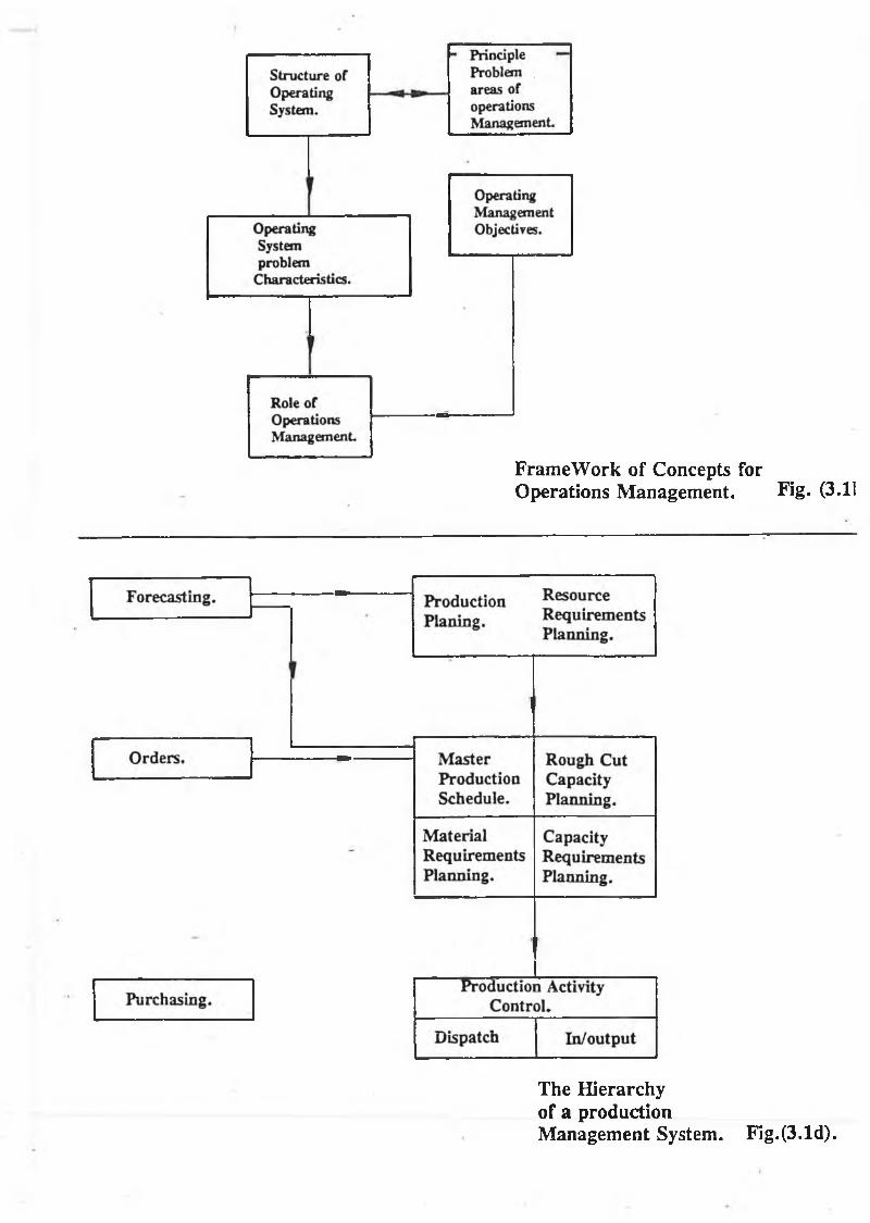
Framework of Concepts for Operations Management. Fig. (3.11

The Hierarchy of a productionManagement System. Fig.(3.Id).

and, operations planning and control. Fig. (3.1b) provides some insight into Wilde’s

ideas.

Groover [26], divides factory planning into four sections:

1. Business Functions 3. Manufacturing Planning

2. Product Design 4. Manufacturing Control

Information flows within this structure are shown in the diagram'(Fig. (3.1c)).

Browne et al [5], speak of production management systems, emphasizing the

hierarchial nature of the structure. Production activity control is forwarded, as that

element of the production management system closest to the production process. Fig.

(3. Id) identifies the hierarchial relationship of the various elements within the

structure.

Depending on which book you choose, the type of structure, designated to the

manufacturing firm will vary, in both terms applied and groupings. The underlying

functions however don’t change, because any manufacturing organization requires

the same undelying functions in order to operate. The essentials of production

control, production planning, inventory control, etc. will always be evident.

3.4 TYPES OF PRODUCTION

The degree of importance afforded to the various functions of organisation structure,

is dependant to some extent on the type of production employed in the plant.

Classification of production types, is also an area, which is subject to a variety of

interpretations.

Wilde [6], identifies three production types, namely:

1. Continuous Manufacture

2. Repetitive Manufacture

3. Intermittant Manufacture

A continuous process may run, 24 hours a day, 365 days a year, and may itself be

of three types.

1. Flow - Chemicals/Cement/Tin Cans.

2. Seasonal Flow - Frozen Vegetables.

3. Flowline - Motor Cars, Television Sets Etc.

A repetitive process, is similar to flowline, in that products are processed in lots,

each product being subject to the same sequence of operations. It is defined by Hall

[31] as:

"Fabrication, machining and assembly and testing of discrete standard

units produced in high volume, or of products assembled in volume

from standard options. It is characterised by long runs or flows of

parts. The ideal is a direct transfer from one work centre to another."

An intermittant process is characterised by small lots, and possibly single products,

made in response to customer orders.

An alternate classification, offered in [5,26] is:

1. Mass Production.

2. Batch Production.

3. Jobbing.

Mass production, is concerned with the continuous, specialised manufacture of

identical products (similar to flowline). Production rates are usually very high,

equipment highly specialised, and usually dedicated to one product.

Batch production is intermediary between mass production and jobbing production is

carried out on small batches, medium size production runs. Each batch being fully

processed, before the next operation takes place. Equipment used, must not be too

specialised, in order that variations in customer requirements may be met (MTS).

Jobbing, is characterised by low volume production runs, with a high variety of

products. This necessitates flexible equipment, and a highly skilled work force.

Products always manufactured against customer orders.

Burbridge in [5], offers another classification of production types:

1. Implosive - Iron Foundry.

2. Process - Cement, Chemicals.

3. Explosive - Electronic Assembly.

4. Combination

Implosive production is typified by products, whereby small varieties of different

materials, produce large variety of products. Process types occur where small variety

of raw material produces a large variety of products. Explosive systems occur, when,

large varieties of raw materials produce small product range.

Irrespective of the type of classification used, as the variety of raw materials, and

product complexity increases, the greater the input required from the various

functions involved. Production control is an easy concept, when, the variety of parts

involved is small, however, as the variety increases production control, becomes more

complex.

3.5 PRODUCTION CONTROL

The production control department, is ideally the link between other departments and

the actual manufacturing process. It processes all the information necessary (Table

3.1) form the various departments, in order to translate customer orders into viable

production schedules.

Scope of Production Control

"Production control, describes the principles and techniques used by Management to

plan in the short term, and control and evaluate the production activities of the

manufacturing organisation". Browne [5].

In an effort to comply with the above definition, the production control department

will perform the following activities:

1. Inventory Control: MRP.

TABLE (3.1): Information Flow To Production Control

I n f o r m a t io n F e d t o P . C o n t r o l S o u r c e D e p a r t m e n t

P r o d u c t io n R e q u ir e d W /O S a le s

D e l iv e r y D a t e W /O S a le s

Q u a n t i t y R e q u ir e d W /O S a le s

M a n u f a c t u r in g M e t h o d R /C P r o d u c t io n P la n n in g

l i m e s , S e q u e n c e s o f O p e r a t io n s

r ; c P r o d u c t io n P la n n in g

M a t e r ia l R e q u ir e d B .O .M . D e s ig n

M a t e r ia l A v a i la b i l i t y I h v . R e e . I n v e n t o r y C o n t r o l

C a p a c i t y A v a i la b le --------- P r o d u c t io n P la n n in g

M a c h in e M a in t e n a n c e ------- M a in t e n a n c e

W /O : W o r k s O r d e r

R / C : R o u t e C a r d

2. Preparation of Working Documents (W/O, R/C, J/T, D/N).

3. Loading, Scheduling.

4. Material Movement Monitoring.

5. Despatch.

6. Progressing.

7. Evaluating Results.

8. Forecasting.

Planning

9. Capacity Planning.

10. Master Scheduling.

11. Labour Planning.

All activities being based on information fed from other departments.

3.6 PUSH AND PULL

3.6.1 In recent years a certain amount of controversy has arisen over the correct

application of the terms push and pull to production control systems.

Orlicky [32], initiated the debate in 1975, by proposing that material requirement

planning (MRP) simultaneously gives rise to both push and pull operation modes.

The push mode, is that of the formal order launch, which by necessity relies upon

possibly inaccurate data - inventory status and otherwise. This gives rise to the

informal pull or expediting mode, in order to ensure that the due date coincides with

the time of actual need.

Schonberger [33], acknowledges that a degree of informality exists within a pull

mode, but says that in reality, a push system is a schedule based system, which

pushes production people into making the parts, and then pushing them onward.

A pull system relies on the assumption that customer orders make up the final

assembly schedule, and parts not on hand are pulled through to meet requirements.

In order to classify two of the commonly recognised pull systems under the heading

push and pull, schonberger considers two. activities - production, and material

handling/delivery. He says of dual card Kanban - Pull system of production

combined with pull system for delivery. Single card Kanban however, used a pull

system for material delivery but production is initiated by a production schedule and

therefore may be recognised as a push system.

Browne [5] adopts the more traditional form of classification: Material requirement

planning logic is that of push, - "Action is taken upon anticipation of Need" -

Kanban Logic is that of Pull- "which requires action upon request."

Papers such as Rice and Yoshikawa [34 ], which refer to both MRP and Kanban as

Pull systems because they both aim to be Just-On-Time, represent a greater attempt

to play with words than finally lay to rest the debate, and proceed with the important

issues to generate and effectively execute valid schedules. Monden [35], summarises

the previous discussion by saying that Push systems require that parts be processed

in accordance with the preceeding work centres requirements, and a Pull system in

accordance with the succeeding processes requirements.

3.6.2 Within manufacturing circles today, two major manufacturing philosophies are

at work. The first of these is the computer based manufacturing resourse planning

(MRP II) system the core of which is the push driven material requirement planning

module. The second philosophy is that of Just-In-Time (J.I.T.), the core of which

is the pull driven Kanban. Much is made of the fact that the J.I.T. philosophy is not

computer-based. This however is a fallacy, and although Kanban itself does not

utilise computers to initiate production or monitor material flow, computers play an

important role in establishing the necessary conditions to make Kanban work (i.e.

production smoothing).

The material requirement planning module, utilizes requirement data, lead time data,

inventory status data, bill of material data to generate production schedules usually

in weekly time buckets for each and every component, sub assembly and end item.

These may or may not contain a degree, of forecasting. In order to initiate

production, within the JIT environment, one schedule is produced daily this schedules

refers only to final assembly items and represents firm customer orders. Within the

MRP push environment production starts at the raw material end, and providing lead

time data is correct, will arrive on time at the next process. The pull environment

requires that a small amount of stock is available at each and every work centre. If

a required item is not available at final assembly (station M), then the required

quantity is removed from station M -l, this also sets production at stage M -l in

process driven by the need to replenish the removed stock.

Manufacturing resource planning carries out the scheduling function with no recourse

to such ideas as group technology (GT) or product families. Batch type manufacture

is the most common type, and a production line may be making the same items all

day. Kanban relies heavily on G.T. and the adage "Make a little bit of everything

every day" describes the production scheduling algorithm for the final assembly, also

referred to as production smoothing. Repetitive manufacturing, which has less

product variety but a greater volume than batch production, but is not quite classified

as mass production is usually associated with Kanban and JIT production.

3.6.3 As stated previously, MRP relies heavily on up-to-date and accurate

information, if this is not forthcoming the formal system breaks down. Individual

process lead times are therefore very important to the success of MRP. With Kanban

however, individual process times and ultimately overall thruput times vary in

accordance with the loading. If the loading is high workers from surrounding work

centres may be brought in and idle machines used to increase the scale of production

and reduce thruput times. Conversely if the loading is light less machines and less

workers are utilized, and so lead times expand. Therefore insiead of lead times

helping to drive the system, the system determines the lead times.

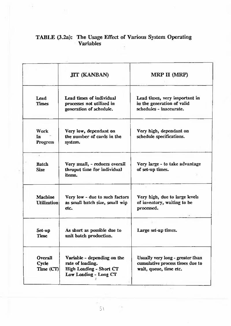
TABLE (3.2a): The Usage Effect o f Various System Operating Variables

JIT (KANBAN) M RP II (MRP)

L e a dT im e s

L e a d t im e s o f in d iv id u a l p r o c e s s e s n o t u t i l i z e d in g e n e r a t io n o f s c h e d u le .

L e a d t im e s , v e r y im p o r t a n t in in t h e g e n e r a t io n o f y a l id s c h e d u le s - in a c c u r a t e .

W o r kI nP r o g r e s s

V e r y lo w , d e p e n d a n t o n t h e n u m b e r o f c a r d s in t h e s y s t e m .

V e r y h ig h , d e p e n d a n t o n s c h e d u le s p e c i f ic a t io n s .

B a t c hS iz e

V e r y s m a l l , - r e d u c e s o v e r a l l t h r u p u t t im e f o r in d iv id u a l i t e m s .

V e r y la r g e - to t a k e a d v a n t a g e o f s e t - u p t im e s .

M a c h in eU t i l i s a t io n

V e r y lo w - d u e t o s u c h f a c t o r s a s s m a l l b a t c h s iz e , s m a l l w ip

e t c .

V e r y h ig h , d u e t o la r g e le v e ls o f in v e n t o r y , w a it in g t o b e p r o c e s s e d .

S e t - u pT im e

A s s h o r t a s p o s s ib le d u e to u n it b a t c h p r o d u c t io n .

L a r g e s e t -u p t im e s .

O v e r a l l C y c le

T im e (C T )

V a r ia b le - d e p e n d in g o n t h e r a t e o f lo a d in g .H ig h L o a d in g - S h o r t C T L o w L o a d in g - L o n g C T

U s u a l ly v e r y lo n g - g r e a te r t h a n c u m u la t iv e p r o c e s s t im e s d u e t o w a it , q u e u e , t im e e t c .

5 \

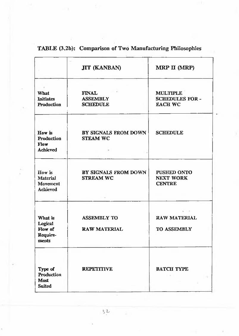
TABLE (3.2b): Comparison of Two M anufacturing Philosophies.

JIT (KANBAN) M RP II (MRP)

W h a tI n it ia t e sP r o d u c t io n

F I N A LA S S E M B L YS C H E D U L E

M U L T I P L E S C H E D U L E S F O R - E A C H W C

H o w isP r o d u c t io nF lo wA c h ie v e d

B Y S I G N A L S F R O M D O W N S T E A M W C

S C H E D U L E

H o w is M a te r ia l M o v e m e n t A c h ie v e d

B Y S I G N A L S F R O M D O W N S T R E A M W C

P U S H E D O N T O N E X T W O R K C E N T R E

W h a t is L o g ic a l F lo w o f R e q u ir e ­m e n ts

A S S E M B L Y T O

R A W M A T E R I A L

R A W M A T E R I A L

T O A S S E M B L Y

T y p e o fP r o d u c t io nM o s tS u it e d

R E P E T I T I V E B A T C H T Y P E

- -

By their very nature, requirement planning systems require a lot of work-in-progress.

The acceptance of long set-up times adds to this problem. Pull systems however,

which concentrate heavily on set-up time reduction can incorporate a very small batch

size. The average work-in progress within the system, is a function of the production

system itself, and is often reduced to a value just above the point at which it would

begin to impede production.

Machine utilizations figures are often quite small using Pull systems when compared

to push. This is due to a number of factors. Firstly, overall requirements are lower,

due to the lack of forecasting within the production schedule. Secondly, smaller

batch sizes, reduce machine utilization. Thirdly, Pull systems only produce what has

been removed, from the system in meeting requirements. The predominant

manufacturing philosophy presently in use in the west is that of manufacturing

resource planning. This is slowly changing however, as manufacturers, aware of the

many benefits to be gained from adopting pull type systems, are beginning to

implement certain pull system elements.

CHAPTER 4 INDUSTRIAL SURVEY

4.1 INTRODUCTION

4 .1 .1 R e v ie w o f I n d u s tr ia l P o l ic y

Ireland finally gained independence in 1922. By that time however industry in the

state had been decimated, with only 4.3% of the population engaged in

manufacturing.

The country’s industrial development from that time to the present day may be split

into two fairly distinct phases. The first, based upon the belief that Ireland could be

made into-

"A self-contained unit providing all the necessities of

living in adequate quantities for the people residing in

Ireland" - Lemass [36].

was inward looking in nature, encouraging a type of import substitution

industrialisation. The main weapon being the indiscriminate use of protectionist

policies. By 1950, after ever increasing balance of trade deficits, it became apparent

that a new approach was required, if indigeneous industry was to break away from

its stagnant position in the technically mature end of industrial markets, into activities,

where barriers to entry were much greater.

The initiation of this new approach was marked by the establishment of the Industrial

Development Authority (IDA), in 1949, followed closely by that of The Irish Export

Board (CTT), and the Grants Board in 1952. Attracting foreign industralists,

advising and encouraging on exports, and supplying non repayable grants, were the

primary functions, of these boards. The introduction of export tax relief (replaced

by low rates of corporate tax) and various finance acts, ensured that by 1960 the

transformation to export orientation was. complete, and that Ireland had become a

favourable shore for foreign investors. Ireland’s subsequent membership of the

European Economic Community (EEC) in 1973, necessitated the introduction of free

trade, but simultaneously provided access to.a large market.

4.1.2 Barriers To Entry For Late Developing Countries

As a late industrializing country, indigenous firms hoping to compete in a wide range

of industrial markets, may face unsurmountable barriers to entry. The most obvious

of these barriers are economies of scale, arising from the fact that the average costs

of well established firms decrease as the scale of production increases. Conversely

a small company starting off will experience barriers due to small production scale,

and hence higher costs.

Larger firms, also have product differentation advantages, arising from brand names,

advertising quality etc. Capital requirements, proprietory technology, learning

curves, and external economies - (suppliers, skilled labour, local market), all combine

to present a significant challenge for any small company thinking of entering a

particular market.

The IDA’s policy of attracting foreign investment, has provided Ireland with the

opportunity to participate (albeit by proxy) in those markets whose entry barriers are

of such great magnitudes that small indigeneous firms have failed to penetrate them

to any degree. The electronics market is one of these areas.

4.1.3 Present Day Statistics

At present the Irish Electronics Industry accounts for nearly one third of annual

exports worth about £4.2 billion, and employs 27,000 people, in 250 firms [37],

Only 45 of these companies however are indigeneous and only one of these appears

in the list of the top one hundred indigeneous firms [36].

4.1.4 The IDA and Foreign Investment

The tradition of direct foreign investment began in the 1930’s, consisting mainly of

English investors, producing for the local market. It was not until the 1950’s that

foreign investment became more export orientated.

The IDA promotes Ireland worldwide as a site, ripe for potential investment. This

often proves difficult for two reasons. Firstly, manufacturing firms generally, are not

anxious to relocate, in order to take advantage of cheap labour etc. Secondly, for

each pool of investors interested in relocating, a large number of newly industrializing

(NIC) or late developing (LDC) countries compete, to act as host nations.

It has been shown in recent years, that foreign investment in late developing countries

worldwide, is confined to occur within one of the three following areas.

1. Basic processing of local resources.

2. Technically mature and standarised labour intensive final products.

3. Relatively simple stages within a longer process of production of

sophisticated goods.

The bulk of foreign investment in Ireland would appear to fall into the latter two

categories. The associated problems are well known: Very little Research and

Development taking place; employment concentration within the lower echelons of

the educational scale, and by virtue of the previous comment, very little transfer of

technology to indigenous industry.

This view of foreign investment in Ireland is reinforced by a survey (1975) by J.

Teeling [36], who says that the majority of electronic firms surveyed-

"Are currently manufacturing satellites, performing partial steps in the

manufacturing process. Skill development, and linkages in,Ireland

have been limited. The electronics industry is a highly skilled industry

worldwide but the activities in Ireland’s electronic industry do not

reflect this."

4.1.5 Why Ireland?

The rapid increase in the numbers of countries competing for foreign investment in

recent years, has required that a potential investor be confronted with slightly more

than low labour costs, ease of access to markets, political stability etc. In the wake

of competition from countries as far apart as Taiwan, and Scotland, Ireland’s

continuing ability to attract foreign investment is surprising.

M. Cronin [37], Head of the Electronics Division in the IDA, puts Ireland’s success

down to availability of skilled labour, low inflationary costs, and finally the tax

incentives and the variety of financial aid packages available. Eoin O’Malley [36]

however, goes slightly further than this, and says that the internationally recognised

efficiency and previous history of such bodies as the IDA and SFADCO, instill a

certain confidence among potential investors. Ireland’s membership of the EEC also

provides insurance against any protectionist tendencies, and guarantees stability.

Finally Ireland’s historical links with both the UK and USA also helps promote

investment.

4.1.6 Ireland and Other Late Developing Countries

O’Brien [38], compares Ireland to both the newly industrializing countries (NIC) in

the Far East - Taiwan and Hong Kong and also small developed countries, such as

Denmark, and the Netherlands. He finds that Ireland has a significantly higher

proportion of foreign multi-nationals, (MNC) than most of these countries. Some of

these countries however, have experienced much greater growth in the their

indigenous sectors than Ireland.

The reasons for this growth in indigenous development (in many cases where the

barriers to entry are high,) is, in most cases due to the successful application of

export orientated policies with a certain degree of protectionism. Korea, as far back

as 1974, frequently imposed exporting and ownership share policies prior to granting

entry permission. The South Korean Government favour loans as a means of foreign

investment, which provides the capital while simultaneously allowing the retention of

indigenous control. Research and Development (R+D) is widely encouraged, as is

the import of foreign technology through licensing. Highly skilled foreigners are

engaged to diffuse technological skills/knowledge down though the industrial ranks.

Taiwan, too, has pursued policies of selective intervention with a great deal of

success. Industries earmarked for indigenous development, are subject to a variety

of tax concessions. The nature of indigenous development in Taiwan is somewhat

different to that of S. Korea or Ireland, being state rather than privately owned.

Singapore’s industrial and development policy, has been rather similar to that of

Ireland in recent years in that it has successfully attracted direct foreign investment,

with little or no impact on indigeneous development. It has begun however to take

need of examples set by Taiwan and S. Korea and is pursuing limited interventionist

policies. Hong Kong, unlike Singapore is not as reliant upon foreign owned

industries, the foreign industries present however have played significant roles in the

development of indigeneous industry via sub contraction. Most of the indigeneous

development however exists in either the more technically mature industrial sector -

clocks, radios etc. traditional third world industry such as textiles. (Similar to

Ireland).

The preceeding discussion would appear to divide late developing countries into two

groups, those that have successfully overcome rigourous barriers to entry in terms of

indigenous development and those that have failed. The pursuance of traditionally

recommended policies for late developing countries generally leads to the latter,

while, deviation from these policies through selective intervention would seem to

cumulate in a more successful conclusion.

TABLE (4.25) Employment Share of Foreign Multinationals in the Electronics Industry

Ireland Scotland Singapore S. Korea Hong Kong Taiwan Denmark Netherlands

(1983)(1978) (1976)(1979) (1978) (1981) (1978) (1981)

90%90%84%45%41%40%37%13%

4.2 RESEARCH OBJECTIVES

4 .2 .1 I n t r o d u c t io n

It has become apparent in recent years that the policies pursued by the IDA have been

unsuccessful in translating the high degree of direct foreign investment to an equable

growth in indigeneous industry. The reasons for this are manifold, and may be dealt

with on two broad levels, namely on an economic, and operating level. In terms of

operations O’Brien [38] proposes that

1. The reluctance of multinationals to engage in R + D in the host

country.

2. The reluctance of MNC to improve production/operation processes in

the host country.

3. Little transfer of skilled labour to indigeneous companies,

profoundly effects both the development and improved competiveness of indigenous

and multinational firms alike. MNC can and do receive help in upgrading production

and operational processes from parent companies. Indigenous firms would hope to

learn from established companies. Where this is not feasible however it may be

possible for these firms to enlist the aid of Universities.

The following study was carried out to assess the need for a University support

group, to upgrade and monitor the development of inventory control systems within

Irish Industry, and in so doing reduce the enormous constraint placed upon indigenous

electronic companies as they try to enter markets where barriers to entry can be very

high.

4 . 2 . 2 R e s e a r c h O b je c t iv e s

The main objectives of this study are:

1. The classification of the Irish electronics industry sector according to, type of

products, type of production, production volume, company size, etc.

2. To identifying the common problems and challanges related to the electronics

industry sector, with respect to their inventory control systems, in particular

MRP implementation.

3. To identify underlying conditions required to make JIT implementation a

feasible proposition for smaller Irish companies.

4. To assess the feasibility of providing technical information and the assistance

with implementing the JIT production concept to these industries.

4.3 RESEARCH METHOD

4 .3 .1 I n t r o d u c t io n

In order to carry out the research objectives described a survey questionnarie was

designed and circulated among one hundred electronic and electrical companies with

manufacturing outlets in Ireland, which were chosen from two lists. One supplied by

the Industrial Development Authority (IDA), and the other by Coras Trachtala (CTT)

the Irish Export Board. The companies were selected purely at random, irrespective

of company size, ownership or demographic situation. Of the original 100 surveys

sent out, only 44 were returned completed. Two companies replied in writing,

declining to participate in the survey, with the remaining 54% failed to reply.

The questionanaire consisted of 50 questions subdivided into six major groups

concerning manufacturing, MRP systems, JIT and their implementation aspects. On

consulting the marketing department, at Dublin City University, it became apparent

that the normal response rates in similar surveys are approximately 33 %, and 44 %

was deemed respectable. No follow-up phone calls were made during the survey,

although previously, each company selected, was contacted to find a contact name

within the company.

4.3.2 Survey Questionnaire

The survey was designed to cover six major areas [Appendix (1)].

Part A: Company Description

Part B: Description of MRP System Status

Part C: MRP Benefits and Costs

Part D: Implementation Problems

Part E: Implementation Approach

Part F: JIT Elements Implementation

4.3.3 N ature of the Response

All returned questionnairs were completed correctly, with the majority of the

questions answered. 11 % of the questionnaires returned were from companies, which

do not have formal MRP systems, although in all cases computerization of individual

elements was evident. It is also interesting to note that 4 % of respondants were in

the process of installing formal systems, and as a result found it difficult to complete

sections, C,D and E.

The remaining returns were in general completely answered, although some of the

individual questions were left unanswered. For the purpose of analysing the data,

unanswered questions were treated as voids.

4.4 SURVEY RESULTS

4 .4 . 1 C o m p a n y D e s c r ip t io n

This initial section of the questionnaire, was designed to provide information

regarding the respective participants, which may be used in later stages to both

classify data and establish a broad profile of the companies involved. This profile

will serve to ascertain the strengths and weaknesses of the various company sub­

sections involved, and allow the analysis of results in relation to the requirements

necessary for successful participation in international markets. The results obtained

in this section are discussed under the various sub-headings found in the survey’s

questionnaire.

Company size

Each respondant was asked to provide information regarding the number of people

the company employed. This information was then subdivided into three categories.

1. Small <50

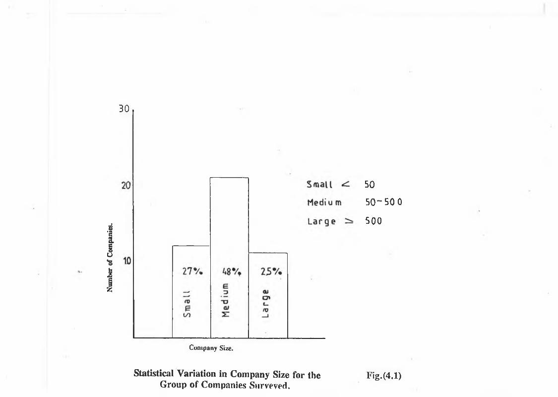
Num

ber

of Co

mpa

nies

.30

Company Size.

Statistical Variation in Company Size for the Group of Companies Surveyed,

50

5 0 - 5 0 0

500

F ig.(4,l)

2. Medium 50 - 500

3. Large >500

Twelve companies, (27%) fell into the first category, twenty one companies (48%)

were classified as medium, while the remaining eleven companies (25%) fell into the

large company bracket. Fig. (4.1) demonstrates the statistical variation in company

size for the group of companies surveyed.

All forty-four companies provided single plant data in answer to this question. The

average number of employees was found to be 267, with a standard deviation of

305.2 and a range from 13 to 1,350. It is evident from the graph that the

approximately 50 % of companies in surveyed fall into the medium size bracket, with

the small and large companies obtaining a fairly equal portion of the remaining

percentage. This is reinforced by a median value which falls into the medium sized

bracket.

Industry Type

Industrial surveys which have been previously carried out conclude that there is a

wide range of companies operating within Ireland, in terms of industry type. These

types were loosely defined to fall within the following groups.

1. Electronics and Computers

2. Electro-Mechanical (Industrial)

3. Electro-Mechanical (Consumer)

4. Electronic Components

Respondants were asked to decide which group best described their product(s). The

analysis of results obtained, led to the distribution shown in Table (4), which includes

classification type, and both number and percentage of respondants which fall under

that classification.

TABLE (4.1): Number\% of Companies Falling Within Each Category.

Product No. ofDescription Companies %

Electronics and Computers 15 34%Electromechanical (Industrial) 14 32%Electromechanical (Consumer) 4 9%Electronic Components 11 25%

Total 44 100%

The electronics and computer sector heads the table with just over a third of all

respondants, closely followed by the electromechanical-industrial sector. Consumer

products ar the least well represented, with only 9% of companies manufacturing for

the consumer market. Electronic component manufacture, is carried out by exactly

one quarter of all respondants. Together, electronic components and computers

makes up just under 60% of all respondants. The various sectors outlined in the table

are listed below together with some of the more common items which belong to the

various sectors.

1. Electronics and Computers

Mini-computer systems, personal computers, microprocessors, large

scale computers, control systems, automatic measuring equipment,

digital integrators, air traffic control systems, energy management

systems, etc.

2. Electro-Mechanical (Industrial)

Line printers, high speed line printers, matrix printers, power supply

units, oxygen analysers, transformers, electric motors,

telecommunication equipment, switch gear etc.

3. Electro-Mechanical (Consumer)

Scales, bathroom scales, hair dryers, electric shavers, fruit mixtures,

smoke alarm systems, electric clocks, movie and slide projectors, etc.

4. Electronic Components

Integrated circuits, printed circuit boards, magnetic heads, potentic

meters, cable harnesses, discrete electronic components, etc.

Table (4.2) shows a list of the industries and/or products that are included in the

group of respondents.

TABLE (4.2): List o f Products and\or Industries

1 C a b le H a r n e s s e s2 C o m p u te r s ( M ln - c o m p u t e r s , w o r d p r o c e s s o r s , p e r s o n a l c o m p u t e r s , la r g e

s c a le c o m p u t e r s , c o m p u t e r s f o r C A D /C A M u s e )

3 C o m p u te r b a s e d p r o c e s s c o n tr o l sy s te m s4 D is c d r iv e c o n t r o l le r s5 D is c r e te e le c t r o n ic c o m p o n e n ts6 D o m e s t ic a p p l ia n c e s7 E le c tr o n ic c o n t r o l p a n e ls

8 E le c tr ic m o t o r s9 f lo p p y d is c s1 0 I n t e g r a t e d c ir c u it s1 1 P o w e r s u p p l ie s12 M a g n e t ic h e a d s1 3 P r in te d c ir c u i t b o a r d a s s e m b ly1 4 R e f r ig e r a t io n u n i t s1 5 S e n s o r s , e le c t r o n ic c o n t r o ls1 6 S m o k e d e te c to r s1 7 T e le c o m m u n ic a t io n e q u ip m e n t

1 8 T e s t e q u ip m e n t1 9 T o u c h t r ig g e r p r o b e s2 0 T r a n s fo r m e r s

From the previous table listing the variety of products available, it is obvious that the

maufacturing costs of these items are many and varied. Adding storage costs to the

already accumulated costs can result in large investments by the manufacturer, with

no guarantee of return. When this investment is balanced against the opportunity cost

of losing sales due to long manufacturing lead times, the outcome results in a decision

to either manufacture to stock (M.T.S.) or manufacture to order (M .T.O.) or both.

Table (4.3) shows the distribution of companies surveyed over these three categories

within each category however, the companies are further divided into those companies

which have material requirement planning systems to carry out inventory control, and

those that do not.

TABLE (4.3): Distribution o f Companies Surveyed with Product Type.

Companies with MRP

Companies Without MR

Total No. Companies

- 4 7 " " No. % No. % No. %Make to Order 20 91 2 9 22 50Make to Stock - - 1 100 1 2Both 19 90 2 10 21 48

The above table demonstrates that a significantly small percentage of company’s

surveyed are operating a strictly make to stock policy. 50% of respondants made to

order, while 48% pursue the dual policy of both make to order and make to stock.

It is interesting to note that the company operating the make to stock policy does not

have an MRP system in operation. Tbe other two categories however, are similarly

distributed over companies which have MRP and those which do not. Approximately

10% of each category operate without MRP and the remainder with the help of MRP.

Manufacturing Types

Over the past few decades, much of the industry which has been attracted to Ireland,

has tended to fall into the assembly bracket. This is generally assumed to require a

low standard of skill, and to do little to promote growth amongst indigenous industry.

Respondants were asked to select the term which best describes their type of

manufacturing and the results obtained are listed below in Table (4.4). Companies

falling within each category, are again subdivided into those companies with

established MRP systems and those companies which carry out inventory control

manually.

TABLE (4.4): Distribution o f Companies Surveyed Over Manufacturing Type.

Companies Companies Total No.with MRP Without MRP Companies

No. % No. % No. %Assembly 25 93 2 1 27 63Fabrication 3 100 - - 3 7Both 10 77 3 23 13 30

One of the forty-four respondants failed to answer this question.

As one might expect, the percentage number of companies who engage in purely

assembly operations, is nearly ten times the number engaged in pure fabrication. The

number who engage in both fabrication and assembly is surprisingly high, just under

half the number engaged in pure assembly. 93 % of those companies, engaged in pure

assembly operations operate MRP systems while 100% of the companies engaged in

pure fabrication, operate MRP systems. When the two types are combined however,

the percentage of the combination group operating without MRP is a large 23%,

compared to only 7% of the pure assembly group.

Type of Process

In keeping with the previous questions, respondants were asked to choose which

process type best describes their industry. Again the distribution of respondants over

these categories is extended to include data regarding non MRP and MRP users.

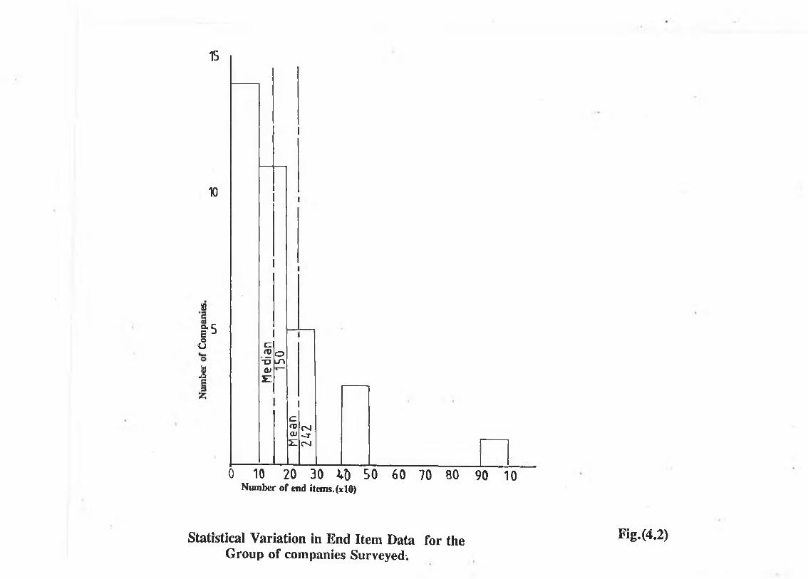
15

10

»

a 5EoU

JSc.COx> air

ol T >

Icrocu2 :

r> l- rOJ

0 10 20 30 M) 50Number of end items. (xlO)

60 70 80 90 10

Statistical Variation in End Item Data for the Group of companies Surveyed;

Fig.(4.2)

TABLE (4.5): Distribution o f Companies Surveyed Over the Process Type.

C o m p a n ie s C o m p a n ie s Total No.W it h M R P W it h o u t M R P Companies

N o . % N o . % N o . %

1 A s s e m b ly T in e 1 8 8 6 3 1 4 2 1 4 82 J o b S h o p 8 8 0 2 2 0 1 0 2 33 C o n t in u o u s 6 1 0 0 - - 6 1 4

C o m b in a t io n o f (1 ) + (2 ) 5 1 0 0 - - 5 1 1C o m b in a t io n (1 ) + (2 ) + (3 ) 1 1 0 0 - - 1 2C o m b in a t io n (2 ) + (3 ) 1 1 0 0 “ — , 1 2

The results of this section shown in Table (4.5) again reiterates that the assembly

process is the dominant force within Irish industry. Assembly manufacture worldwide

is characterized by large volume production runs of highly standardized products.

Labour skills are usually low, and tooling and equipment very specialized leading to

an absence of flexibility on all fronts. The number of facilities engaged in a job shop

type process is just less than half engaged in the previous process types. Equipment

is less specialized in this environment leading to greater flexibility, and labour skills

are also required at a much higher level. The number of companies involved in

continuous or batch production is just under a third the number involved in assembly

manufacture. 11% of the overall sample engages in both job shop and assembly-line

manufacture.

Three of the five companies identified as not having MRP systems fall into the

assembly line group and two into the job shop group. Note that the percentage of

non-MRP ’ companies within the job shop group is significantly higher than the

percentage within the assembly line group, as might be expected, due to the nature

of job shop type processes - high product differentiation.

The remaining data collected pertaining to product descriptions, and assessment, also

have bearing on the performance of the material requirement planning system. This

data falls' into three parts, - firstly the number of end-items or products which appear

regularly on the master production schedule. Secondly, the number of individual items

which appear in the bill of material. Finally, the number of levels incorporated into

the bill of material.

End item (product) data

Of the forty-four companies surveyed, four companies failed to provide end item

figures, and of the forty replies, four of these fell outside the range of the graph.

(Fig.4.2). The mean of the graph is 242, and the standard deviation is 216. The

median of both graph and data is 150. The range of end items is 9 to 7000. If the

four end item figures which fall outside the range of the graph are included in the

mean calculation, the resultant mean is 718, almost three times the mean with these

values left out. The standard deviation with these values included increases sevenfold

to 1493.

Because 90% of data (36 companies) fall within the range specified on the graph, it

may be concluded that the four figures which fall outside the range specified are

biasing both the mean and the standard deviation and will therefore be ingored.

Part number data

The response rate to the part number question mirrors that of the end product data,

with four voids. In this case however, only three of the results obtained lies outside

the range of the graph. (Fig 4.3). The mean of the graph is 2969, and when the

figure outside the graph range are included it increases to 3150. The standard

deviation of the graph is 2402, and rises to 3330, when all the data is included,

included. The median of the complete data set is 1800 and that of the graph 1200.

Because 93% of the data falls within the graph range, both the mean and standard

deviation of the graph can be taken as that of the complete data set.

Bill of materials

43 of the respondants answered the question regarding the number of levels in their

Num

ber

of C

ompa

nies

.

u

12

10

80)2a>ca<u

2 .

in

m

'o0CH

croXJ

1 Q j31

1 2 3 4 5 6 7Number of Parts(xlOOO).

Statistical Variation in Part No. Data for the Group of Companies Surveyed.

8 9 10 12

Fig.(4.3)

bill of material. (Fig 4.6). The range of values obtained varied from one to 13. The

mean of the data is 4.51 and the standard deviation 2.36.

4.4.2 The state of MRP systems in Ireland

The preceding section was used to establish the background of the companies involved

in the survey and emphasizes the nature and range of these companies. This section

presents the results pertaining to the extent of computerization within these companies

and also the degree to which information being input and processed by machines is

accurate. It is not possible to assess the performance of computerization in relation

to plant operation unless a certain confidence level, in terms of data accuracy is

reached.

Extent of computerization

In order to evaluate the extent of computerization across a spectrum of individual

tasks, respondants were asked to identify the areas in which tasks were carried out

manually or with the aid of a computer. These tasks are arranged (Table 4.6) in order

of decreasing percentage computerization. Percentages were awarded on the basis of

a very simple system, whereby, if the task was computerized, it scored a one, and

since forty-four companies responded, the maximum score for any task was forty-

four. Parts explosion, for example was marked computerized on 28 of the possible

forty-four surveys and assumes fourth position in the list, with a score of 63%.

From Table (4.6), it can be seen that the most prevalent computerized task is the

inventory stock system. The purpose being solely to monitor inventory in\out and

through the system. When material comes in to the factory it is entered into the

system and when it leaves it is removed from the "live" system. A bill of material,

parts explosion\purchasing and order release, are all vital elements of an MRP system

and yet the extent to which computers are used to carry out these tasks vary

significantly. Between 30% to 48% of companies carry out these tasks manually.

Comparing these figures to those of average number of products and part numbers

242, 2969, respectively would seem to imply that some of these companies could well

1 2 3 4 5 6 7 8MRP Levels.

Statistical Variation in MRP levels For the Group of Companies Surveyed.

Fig.(4.6)

do with an injection of computerization.

TABLE (4.6): % Computerization o f Individual Elements

M R P E le m e n t % C o m p u t e r iz a t io n

I n v e n t o r y s t o c k s y s te m 8 1 %B il l o f m a te r ia l 7 0 %P u r c h a s in g 68%F a r t s e x p lo s io n 6 3 %

O r d e r r e le a s e 52 %M a s t e r p r o d u c t io n s c h e d u le 4 5 %F o r e c a s t in g e n d ite m s 3 8 %S h o p f lo o r c o n tr o l 3 1 %C a p a c it y p la n n in g (r o u g h c u t) 2 9 %O p e r a t io n s s c h e d u lin g 2 7 %

Less than half the respondants operate a computerized master production schedule and

less than a third, a computerized capacity planning module. A computerised master

production schedule is often used interchangeable with capacity planning to perform

a type of capacity planning and it is surprising to see both of these tasks at such low

positions in the table. Computerised shop floor control, a vital link in closed loop

MRP also takes up a very low position in the table, at 31% computerization. This

would seem to imply that MRP users are using their systems for simple tasks such

as order launching, ignoring some of the more advanced facilities.

Computerization vs Company Size

In order to compare the percentage overall computerization of the respondants, a

weighting factor must be introduced. Respondants were asked to specify whether the

individual tasks listed were carried out manually or on a computer. When a task was

performed maually it scored a one. Otherwise it scored a two. The maximum score

for any respondant is 20, which indicates that all tasks are computerized. Dividing

the range 0-20 into five sections,

0-3, 4-7, 8-11, 12-15, 16-20.

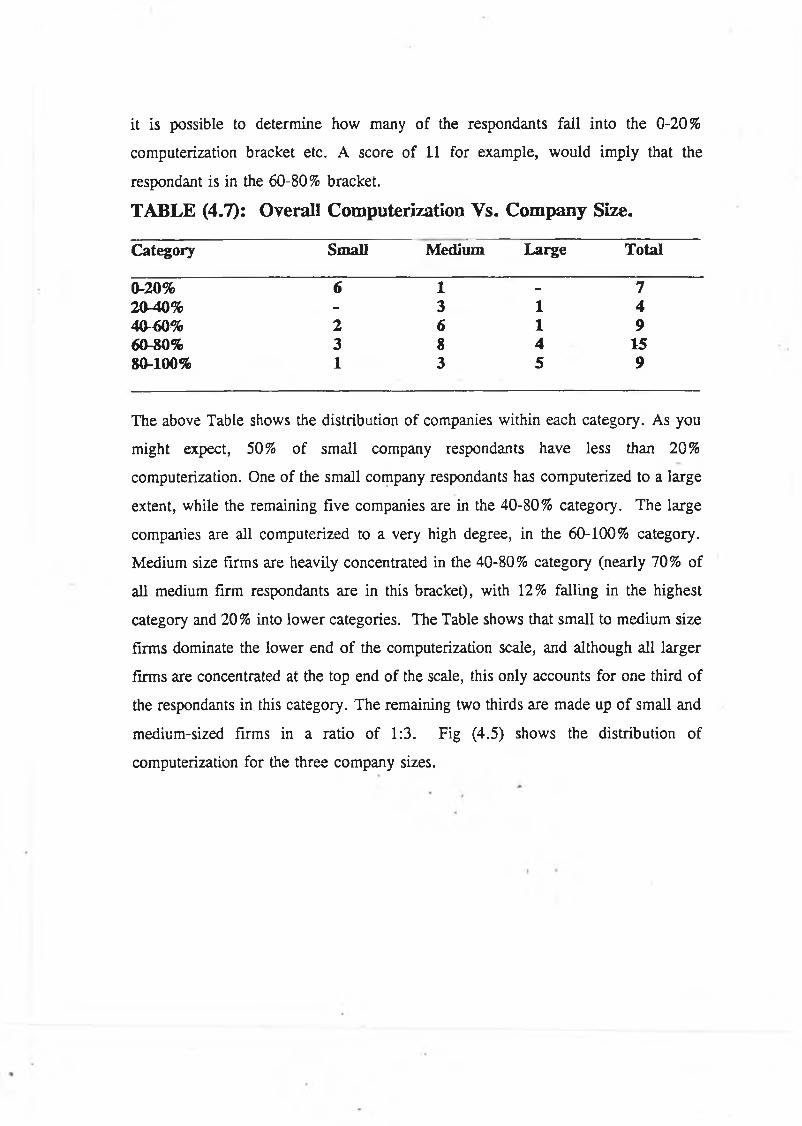
it is possible to determine how many of the respondants fail into the 0-20%

computerization bracket etc. A score of 11 for example, would imply that the

respondant is in the 60-80% bracket.

TABLE (4.7): Overall Computerization Vs. Company Size.

C a te g o r y S m a ll M e d iu m L a r g e T o t a l

0-20% 6 1 - 7

2 0 -4 0 % - 3 1 4

4 0 -6 0 % 2 6 1 96 0 -8 0 % 3 8 4 1 58 0 -1 0 0 % 1 3 5 9

The above Table shows the distribution of companies within each category. As you

might expect, 50% of small company respondants have less than 20%

computerization. One of the small company respondants has computerized to a large

extent, while the remaining five companies are in the 40-80% category. The large

companies are all computerized to a very high degree, in the 60-100% category.

Medium size firms are heavily concentrated in the 40-80% category (nearly 70% of

all medium firm respondants are in this bracket), with 12% falling in the highest

category and 20% into lower categories. The Table shows that small to medium size

firms dominate the lower end of the computerization scale, and although all larger

firms are concentrated at the top end of the scale, this only accounts for one third of

the respondants in this category. The remaining two thirds are made up of small and

medium-sized firms in a ratio of 1:3. Fig (4.5) shows the distribution of

computerization for the three company sizes.

10

8

6 I-

U

2

L a r g e

V)a j‘ctD CL

' E oLJoo

10

8

6

4

2

t)

86

2

Medium

Sm a U .

2 0 6 0 80 100 % computerization.

% overall Computerization Vs. No. of Companies.

*

F ig .(4 .5 )

TABLE (4.8): % Overall Computerization Vs. Product Description.

C a te g o r y 0-20% 2 0 -4 0 % 4 0 -6 0 % 6 0 -8 0 % 8 0 -1 0 0 %

E le c t r o n ic s /c o m p u t e r s - 1 5 5 4E le c t r o /m e c h a n ic a l , '

( In d ) 3 - 7 2 2E le c t r o /m e c h a n ic a l ,(C o n s ) 1 - 1 1 1E le c t r o n icc o m p o n e n t s 3 3 - 3 2

T o t a l 7 4 9 1 6 9

The above Table (4.8) differs from the previous Table, in that the various percentage

computerization categories are now distributed over the various product description

categories. Electronics and computers category are fairly evenly distributed from 40-

100% with one company or 9% of this group falling below 40% The second

category, electro-mechanical industrial has a greater range of computerization varying

from 0-100%, with nearly 50%, of data falling into the 60-80% group. Electro­

mechanical consumer fails to reach a peak, across the spectrum of computerization

categories. Electronic components has at least one company falling into each

category. 50% of this group falls below 40% computerization while 40% of data has

60% or greater computerization.

Electronics and computers and electromechanical (Ind.), dominate the 40-100%

computerization categories, electronic components, the 20-40% category and both

electro-mechanical (Ind.) and electronic components the less than 20% category. Fig.

(4.4) describe the % computerization distribution for the various product descriptions.

4

2

6Electronic Components.

10 r

8

6

k

2

V

8

6

U

2

E lec t ro -Mech(Cons . ) .

Eie c t ro-M echdrr.d.l.

10 r

8 6

4

2

E le c t ron ic s and C o m po n en t s .

0 20 A0 60 80 100% computerization.

% Overall Computerization Vs. Product Description. Fi g. (4.4)

A ccuracy o f D ata

Respondants were asked to comment on the degree of accuracy present in the various

tasks listed below. Accuracy is very difficult to quantify, but the following system

was developed to measure it approximately. The system is an extension of the

previous one used to measure degree of computerization. Respondants were asked to

choose one of the following adjectives to describe the accuracy of the individual

tasks: poor, fair, good, and excellent. A number from one to four was assigned to

each respectively. The maximum score for any task was therefore,

4x (44-number of voids)

when accumulated over all the returned questionnaires. Master production scheduling

for example, with a total score of 94, and seven voids, was placed fourth highest in

the list with a percentage accuracy of (94)(/4(44-7)) =63.5% The Table below

summarizes the results.

T A B L E (4 .9 ): Percentage O ve ra ll A ccu racy O f D a ta .

Description Poor Fair Good Excellent % O verall accuracy

B ill of m aterial 5 17 44 34 77%Tnv. records 7 14 45 33 76%Production 1.tim es 10 33 38 18 66%M aster production scheduling

11 38 38 14 64%

Vendor lead tim es 18 26 44 13 63%Shop floor control 13 38 36 13 62%Capacity planning 11 36 44 8 62%M arket forecasts 28 44 24 4 50%

The table shows the bill of material heading the pole for data accuracy, with

inventory records data just behind. Both of these two tasks are vital to the success of

MRP and as such atttempts should be made to keep updating these tasks rather than

just allowing them to become’static in the system. Production and vendor lead times

scores, underline the problem associated with obtaining accurate lead times. In its

attempt to match batch size with demand from the market, MRP, in creating a variety

of production lots, ultimately varies the lead time, causing a mismatch between MRP

output and actual requirements. Lead times are not independent of batch size and

should not be regarded as such. Market forecasting and hence Master Production

Scheduling have also scored a low degree of accuracy, with the former coming last

in the list, with only 50% accuracy. Shop floor control scores a similar degree of

accuracy as that calculated for other MRP tasks, such as master production scheduling

etc., which raises the question as to why closed loop MRP, utilizing feedback from

the shop floor is not as widespread as other MRP tasks, considering it is as accurate

as some of the more prevalent MRP tasks.

TABLE (4.10): Data Accuracy Vs. Firm Size.

% A c c u r a c y S m a ll M e d iu m L a r g e T o ta l

< 2 5 % - - - -

2 5 -5 0 % 4 8 - 125 0 -7 5 % 4 1 5 5 2 47 5 -1 0 0 % 2 4 - 6

Table (4.10), similar to the overall computerization Table, shows the distribution of

firm size, with percentage overall accuracy. The figures in the Table are arrived at

in a similar fashion by assuming the top score per individual survey is 4 x 8 = 32,

and then, dividing the range 0-32 into appropriate ranges. Two voids were

encountered in this section. Notice that no respondants have less than 25% overall

accuracy. 28% of respondants fall into the 25-50% accuracy category and over 50%

into the 50-75% accuracy. Only 14% of the respondants have between 75-100%

accuracy. It is interesting to note that while both small and medium size firms have

wide ranging accuracies from 25-100%, large firms are wholy concentrated in the 50-

75% bracket, which is also the bracket in which the number of medium-sized and

small firms peak.

M R P F e a tu r e s

Respondants were also asked to answer questions regarding the special features of

their respective MRP systems. The number of voids encountered in this section was

surprisingly high, varying from 17 when asked about the update method, to 10 for

the questions relating to pegging, cycle counting and lot sizing. Table (4.12) below

summarizes the results obtained.

TABLE(4.12): MRP Features Vs. Number o f Companies.

F e a t u r e N o . %

U p d a t e R e g e n e r a t iv e 1 3 4 8m e t h o d N e t C h a n g e 1 4 5 2

P e g g in g 1 9 5 6C y c le c o u n t in g 2 2 6 5L o t s iz in g 1 7 5 0

Respondants were split fairly evenly between regenerative and net change update

method. Of the other three features, cycle counting is the most prevalent, with 65%

of respondants employing this feature. Lot sizing is the least prevalent, with only half

the respondants exhibiting this much publicised feature. 21% of respondants (7

companies) employ none of these features, and the same number utilize two while 32

(11) companies use all three features.. Each of these features have proved useful in

the successful implementation of MRP and it is surprising to see them all in such a

limited operating environment.

Table (4.13) distributes the number of features per company over firm size. It may

be seen that only 12% of all small firms have all three features compared with one

third of medium firms, and 43% of large firms. In fact the Table demonstrates that

small firms are more likely to have no added features. 10% of medium firms also

have no added features, but all large firms’ respondants have at least one feature.

TABLE (4.13): Number of Features Vs. Firm Size.

N o . o f f e a tu r e s S m a ll M e d iu m L a r g e T o t a l

T h r e e 1 6 3 1 1T w o 1 5 3 9O n e 1 5 1 7N o n e 5 2 7

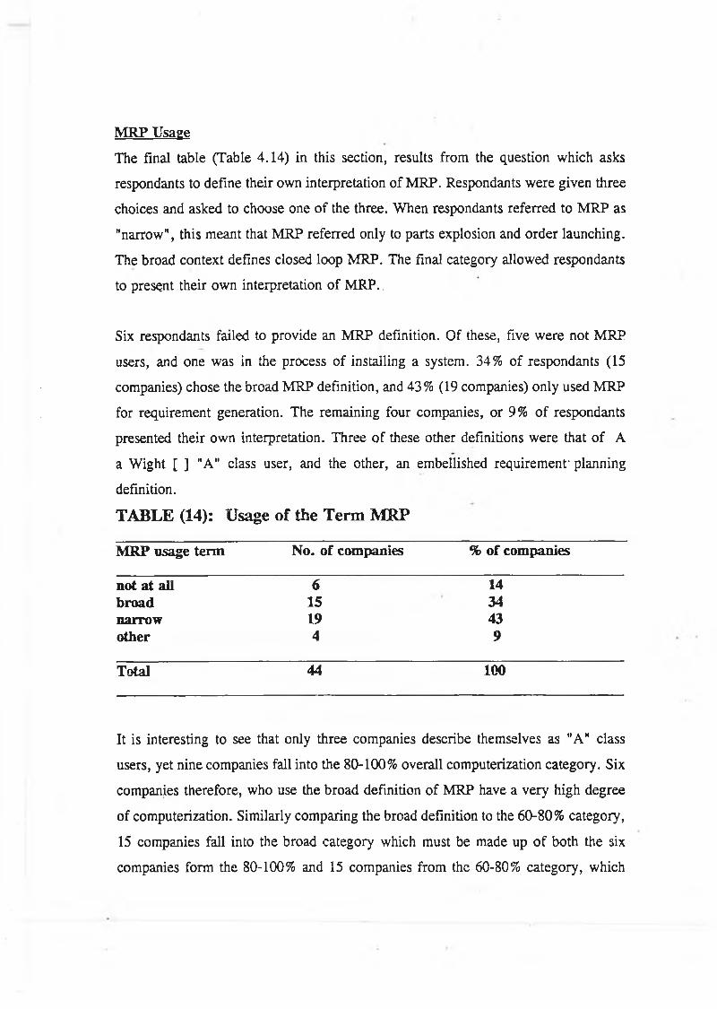
M R P U s a g e

The final table (Table 4.14) in this section, results from the question which asks

respondants to define their own interpretation of MRP. Respondants were given three

choices and asked to choose one of the three. When respondants referred to MRP as

"narrow", this meant that MRP referred only to parts explosion and order launching.

The broad context defines closed loop MRP. The final category allowed respondants

to present their own interpretation of M RP..

Six respondants failed to provide an MRP definition. Of these, five were not MRP

users, and one was in the process of installing a system. 34% of respondants (15

companies) chose the broad MRP definition, and 43% (19 companies) only used MRP

for requirement generation. The remaining four companies, or 9% of respondants

presented their own interpretation. Three of these other definitions were that of A

a Wight [ ] "A" class user, and the other, an embellished requirement'planning

definition.

TABLE (14): Usage of the Term MRP

M R P u s a g e t e r m N o . o f c o m p a n ie s % o f c o m p a n ie s

n o t a t a l l 6 1 4

b r o a d 1 5 3 4n a r r o w 1 9 4 3o th e r 4 9

T o ta l 44 100

It is interesting to see that only three companies describe themselves as "A" class

users, yet nine companies fall into the 80-100% overall computerization category. Six

companies therefore, who use the broad definition of MRP have a very high degree

of computerization. Similarly comparing the broad definition to the 60-80% category,

15 companies fall into the broad category which must be made up of both the six

companies form the 80-100% and 15 companies from the 60-80% category, which

implies that six companies which supplied the narrow definition have a very high

percentage computerization for that definition. The 19 companies which fall into the

narrow category are scattered in the 20-80% overall computerization, with nearly

twice as many companies falling into the 40-60% category. This lack of uniformity

in describing the state of MRP systems underlines the need for a concise classification

system.

4 .4 .3 M R P B e n e f i t s

This brief section chronicles the benefits in percentage terms which MRP

implementation brings about. Respondants were given a list of four potential benefits,

and were asked to give each one a mark from one to four. The numbers stand for

little, some, much and very much, respectively. The system then used to work out

percentage benefits, mirrors that of the corresponding tables in the other two sections.

Table (4.15) also exhibits the percentage scored by the various categories offered.

TABLE (4.15): Percentage Benefits Derived From MRP

B e n e f i t s l i t t le /n o n e

s o m e m u c h v .m u c h o v e r a l l s c o r e %

I m p r o v e d c u s to m e r s a t is f a c t io n 9 4 0 3 7 1 4 64% .

B e t t e r p r o d u c t io n s c h e d u l in g 3 3 1 46 1 7 69%

I m p r o v e d m a n . l e a d t im e s 1 5 2 9 4 7 9 63%

B e t t e r in v e n to r y c o n tr o l 1 7 3 7 46 85%

The Table is headed by better inventory control, scoring 85 % out of a possible 176.

Relating inventory control to inventory stock systems and bills of material, percentage

computerization scores, it is obvious that the majority of respondants realize that

much is to be gained by their computerization. Improved production scheduling is

second in the list, with a score of nearly 70%. It would appear however from

percentage computerization figures that this task is the least likely to be computerized

appearing last on the list.

Improved customer satisfaction and improved manufacturing lead times, score

approximately the same in the benefit Table. Considering only 43% of respondants

operated either closed loop control MRP systems, or a more sophisticated form of

MRP, it may be assumed that quite a high percentage of respondants are finding

improved customer relations from implementing more rudimentary MRP. Relating

improved production lead times to the measure of accuracy afforded to the latter, it

is interesting to see that both score approximately the same - 66% accuracy, 63%

improvement in lead times. Of course the former relates more to the accuracy of the

lead times held within the system, and the second to actual practical production lead

times. The difference between the two scores might be expected to be wider, due to

the cumulative effects of inaccurate lead times at each station.

TABLE (4.16): Benefit Overall From MRP System

C a t e g o r y S m a ll M e d iu m L a r g e T o t a l

0 -2 5 % - - - -

2 5 -5 0 % 2 1 35 0 -7 5 % 4 10 1 1 57 5 -1 0 0 % 2 12 2 1 5

The Table 4.16 distributes overall benefits over the various firm size category. The

vast majority of companies stated an overall benefit of over 50%. Only 3 companies

fell below the 50% mark.

Both small and medium firms were spread over the 25-100% range, which compares

to the accuracy ranges, also encountered in this firms. The range of percentage

benefits encountered in large firms is wider than that of overall accuracy, being

concentrated in the 50-75% range in the latter, and 50-100% in the former. Accuracy

may therefore be related to benefit. Each firm size however peaks at a slightly higher

percentage benefit than it does in the accuracy Table.

4 . 4 . 4 I m p le m e n t a t io n P r o b le m s

Much has been written about the ideal method of approach, when initiating the

changeover from manual to the computerized manufacturing control system. Many

companies operate both systems simultaneously, for a time, so that a certain level o f

confidence can be achieved in the computerized system before rejecting the old

manual system.

A list of commonly recurring problem areas has been compiled from literature.

Respondants were then asked to comment on the degree to which the area had caused

problems. Four choices were offered, little or none, some, much, very much,

corresponding to one to four respectively. A similar marking scheme to the one

previously used was employed to produce the following Table. (Table 4.17).

The percentage number of companies falling under each heading are also listed.

TABLE (4.17): Individual Implementation Problems Vs. % Magnitude of Problem

P r o b le mT y p e

L it t le S o m e M u c h V e r y m u c h % o v e r a l l d e g r e e t o w h ic h it c a u s e d p r o b le m s

M a s t e r p r o d u c t io n s c h e d u le 2 4 3 3 2 4 1 8 6 1 %

L a c k o f s u i t a b le s /w a r e 2 3 4 5 2 6 5 4 %

P r o d u c t io n le a d t im e s 2 6

L a c k o f 3 1e x p e r t is e

C o n s tr a in t o f h /w a r e 5 3

C o s t o f s /w a r e 5 0

5 7

3 5

1 9

26

1 7

2 3

1 9

12

11

9

i l

4 8

4 8

4 6

4 6

The problems, were basically of two types: - those relating to MRP tasks - master

production schedule and production lead times, and those relating to the MRP

operation and installation.

Master production scheduling heads the list, scoring 61%, justifying its place in the

list, It is interesting that production lead times proved to cause significantly less of

a problem than master production scheduling, scoring just under 50%.

Unsuitable software caused the greatest problems in relation to MRP operation and

installation, followed by lack of expertise, within the company. The relationship

between both of these problems is interesting. If experts in the field of MRP were

employed within the company, this might possibly eliminate the purchase of

unsuitable software. It would also avoid the purchase of unnecessary hardware, when

the system requirements exceeds that of present hardware restrictions. The cost of

buying software scores the lowest in the list, however this would be exacerbated with

the purchase of unnecessary software.

Respondants were also asked to provide information on any other major problems

encountered during MRP implementation. The replies were many and varied, loosly

falling into three subsection. Table (4.18) lists the replies.

TABLE (4.18): M ajor Problems Encountered During M RP Implementation.

S o f tw a r e : D o e s n o t h a v e m u lt i - c u r r e n c y c a p a b i l i t y .L a c k o f a v a i la b le s o f tw a r e f o r f a b r ic a t io n .I n a b i l i t y t o in t e g r a t e w ith o th e r s y s t e m s .O n ly h a v e r e g e n e r a t iv e M R P

P e o p le r e s o u r c e : N o M R P c h a m p io n .R e lu c t a n c e o f s t a f f t o c h a n g e .L a c k o f e x p e r t is e i n r a w m a te r ia l p la n n in g a n d M R P L a c k o f s k i l le d p e r s o n n e l.L a c k o f u n d e r s t a n d in g o f n e e d f o r d is c ip l in e a n d fo r m a l p r o c e e d in g s .L a c k o f m a n a g e m e n t c o m m it tm e n t .A b i l i t y to m a n a g e c h a n g e a n d t r a in in g r e q u ir e m e n ts .L a c k o f c o m p a n y -w id e a c c e p ta n c e .P r o b le m w ith c o n v in c in g p a r e n t c o m p a n y o f r e q u ir e m e n t s .

D a t a a c c u r a c y : T r a n s f e r r in g d a ta f r o m o ld t o n e w s y s t e m .P o o r in i t ia l d o c u m e n ta t io n .P o o r d a t a in te g r i ty .P o o r s a le s f o r e c a s t s .B i l l o f m a t e r ia l s tr u c tu r e n o t c o n d u c iv e t o s y s t e m .L a c k o f in t e g r i t y b e tw e e n s to c k r o o m a n d s h o p f lo o r .

The replies relating to software reiterate the need for deciding upon the exact

requirements of the company system before making the choice to purchase\develop

software.

In order to complete a successful changeover to computerization, the total

committment of all the people involved is required, under the guidance of an "MRP

champion". All replies relating to the people resource underline this need.

The need for accuracy, when implementing MRP is qualified by the adage "rubbish

in, rubbish out", in relation to data. The inability to keep track of stock, once issued

to the factory floor, prevents any sort of backflushing procedure, to stock count and

the formal discipline of the MRP system breaks down. This and other data accuracy-

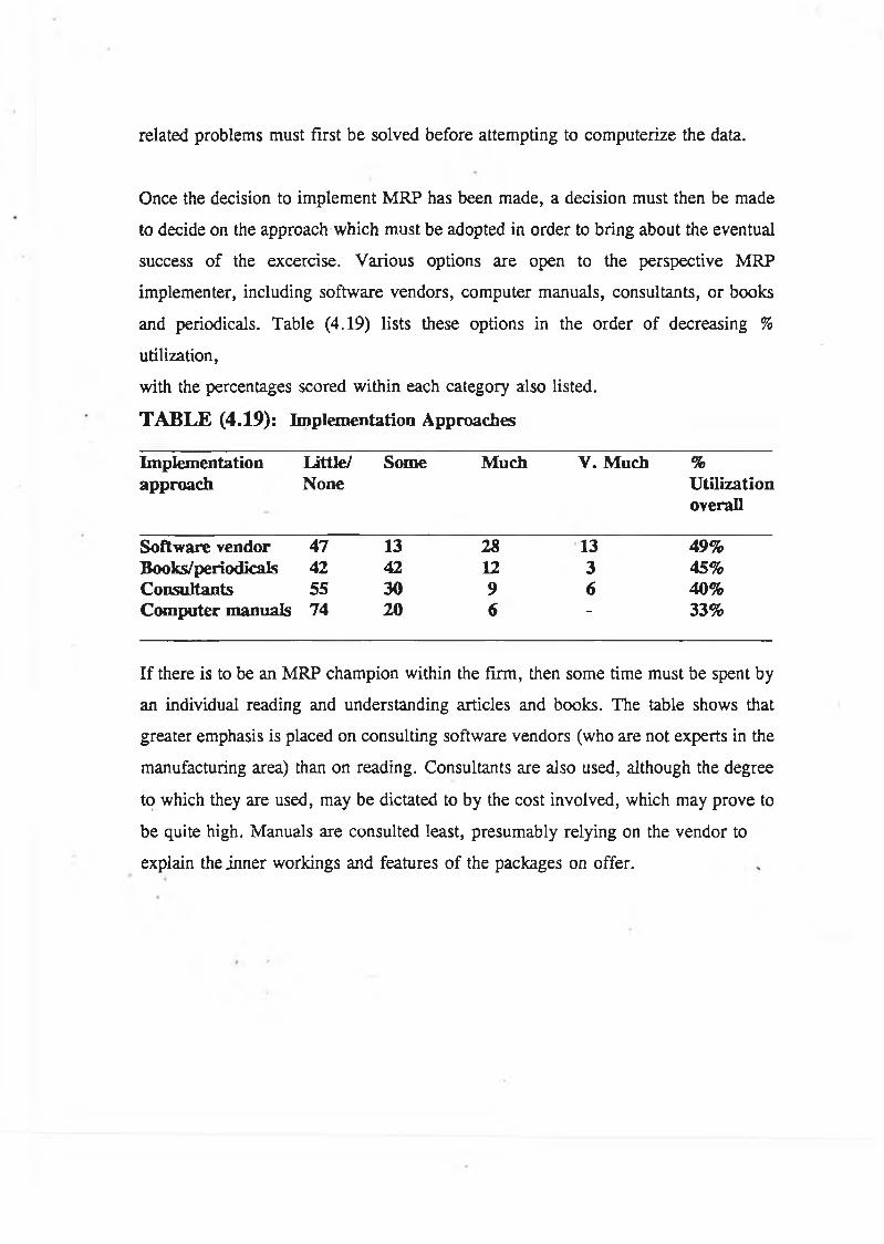
related problems must first be solved before attempting to computerize the data.

Once the decision to implement MRP has been made, a decision must then be made

to decide on the approach which must be adopted in order to bring about the eventual

success of the excercise. Various options are open to the perspective MRP

implementer, including software vendors, computer manuals, consultants, or books

and periodicals. Table (4.19) lists these options in the order of decreasing %

utilization,

with the percentages scored within each category also listed.

TABLE (4.19): I m p le m e n t a t io n A p p r o a c h e s

I m p le m e n ta t io na p p r o a c h

l i t t l e /N o n e

S o m e M u c h V . M u c h %U t i l i z a t io no v e r a ll

S o f t w a r e v e n d o r 4 7 1 3 28 1 3 4 9 %B o o k s /p e r io d ic a ls 4 2 4 2 12 3 4 5 %C o n s u lta n t s 5 5 3 0 9 6 4 0 %C o m p u t e r m a n u a ls 7 4 20 6 - 33 %

If there is to be an MRP champion within the firm, then some time must be spent by

an individual reading and understanding articles and books. The table shows that

greater emphasis is placed on consulting software vendors (who are not experts in the

manufacturing area) than on reading. Consultants are also used, although the degree

to which they are used, may be dictated to by the cost involved, which may prove to

be quite high. Manuals are consulted least, presumably relying on the vendor to

explain the inner workings and features of the packages on offer.

I

TABLE (4.20): Software Source

S o u r c e % U t i l iz a t io n

V e n d o r s u p p l ie dw it h m o d if ic a t io n 5 5 %

V e n d o r s u p p l ie dw it h o u t m o d if ic a t io n 2 4 %

D e v e lo p in te r n a l ly 12%B o th 9 %

Table (4.20) above, lists the various sources of software available and the

corresponding percentage, indicating the degree to which the respective sources were

utilized. The majority of companies approached vendors, -79% of the sample 70%

of which required a degree of customization. Only a very small percentage developed

their own system - 12% of the sample, which is consistent with the very small

number of companies who had an MRP expert or "champion" among their personnel.

Only 9 % of companies jointly used their expertise on their own manufacturing control

system, and the vendors expertise on the packages available, and customization

required.

4 . 4 . 5 JT T I m p le m e n ta t io n

MRP originated and developed in America, and slowly filtered through to Europe and

the rest of the world. In a similar fashion, Just-In-Time manufacturing techniques

originated in Japan, and are slowly becoming known in the rest of the world. Just as

it took time for companies to initially realise the benefits of computerization and

begin implementation, manufacturers are wary of JIT techniques and resistant to try

to implement them.

From Table (4.21) it is possible to compare the number of companies who are aware

of JIT and its various elements, and those which have actually tried to implement

some of those elements. Of the 70% of respondants who had prior knowledge of JIT,

27 of these companies had begun implementation. One third of these 27 companies

hoped to further implement JIT in the future, while the remaining two thirds had

decided to curtail their JIT activities. Just over half the companies which had not as

yet embarked on a JIT program intended to in the future, while the remaining 7

companies, had no intention to at present.

TABLE (4.21): JIT Implementation Statistics

C o m m e n t N o . o f c o m p a n ie s % o f t o t a l s a m p le

- J I T t e c h n iq u e s m a y b e 3 0 7 0 %s u c c e s s f u l ly im p le m e n t e d in t h e ire n v ir o n m e n t .- h a v e im p le m e n t e d s o m e J I T 2 7 63 %t e c h n iq u e s .- in t e n d t o im p le m e n t f u r t h e r 9 21%

t e c h n iq u e s in t h e f u t u r e .- d o n o t in t e n d t o im p le m e n t f u r t h e r 1 8 4 2 %

t e c h n iq u e s .- h a v e n o t im p le m e n t e d a n y J I T 7 16 %t e c h n iq u e s b u t in t e n d t o in t h ef u t u r e .- d o n o t in t e n d to im p le m e n t 9 21%

a n y t e c h n iq u e s .

Table (4.22) demonstrates the number of companies who have or intend to embark

on a JIT program distributed over firm size. Of the 27 firms which have a JIT

program, the majority of firms (17 are medium-sized), while the remaining 10 firms

are split evenly between large and small firms. 4 medium-sized firms intend to

embark on a JIT program in the future, ensuring that all or 100% of the medium

firms have or will have JIT programs. Only 7 of the 12 small firms have, or will

have JIT programs, and a surprisingly low 50 % of large firms have or intend to have

a program.

TABLE (4.22): JIT Implementation Vs. Company Size

C o m m e n t s m a l l m e d iu m la r g e t o t a l

- h a v e a lr e a d y im p le m e n t e d s o m e J I T t e c h n iq u e s . 5 1 7 5 2 7

- h a v e n o t a lr e a d y im p le m e n t e d J I T b u t

in t e n d t o in t h e f u t u r e . 2 4 1 7

As mentioned previously JIT is a manufacturing philosophy, which encompasses the

complete manufacturing procedure. As such, JIT has many facets, all the techniques

all of which are listed in Table (4.23). They deal with tasks as varied as quality - zero

defects - to employee training, through to developing uniform work loads, on the

manufacturing lines.

When companies first decide to implement some JTT techniques, their interpretation

of the techniques with which to start may not coincide. This point is demonstrated in

Table (4.23), which shows the percentage of the total sample, who intend or have

already implemented the various techniques. This varies from 47% to 12%

implementation at present. It is interesting to see that the JIT delivery technique leads

the Table, bearing in mind that we are an island nation. Cross training of employees

is second in the list, with 40 % of companies already operating a scheme and another

19% planning to in the future. Controlling material flow through the use of signals

(card etc.) instead of relying purely on the requirement planning output is also

implemented to a high degree, with 38% of companies using Kanban techniques. One

of the more popular terms in Irish manufacturing circles today is ISO 9000, and

quality standards which accounts for 37% of the sample pursuing the zero defects

goal. The ultimate goal of any company trying to achieve manufacturing excellence

through JIT is the ability to produce unit batches efficiently. This cannot be achieved,

unless set-up times per job are reduced or eliminated. With this in mind, it’s

interesting to see that the percentage of companies trying to reduce set-ups, is 10%

lower than that number who are aiming for JIT delivery.

TABLE (4.23): Implementation Techniques Vs. % Implementation

T e c h n iq u e % im p le m e n ta t io n a t p r e s e n t

% im p le m e n t a t io n i n t h e f u t u r e

J I T d e l iv e r y 4 7 % 2 6 %C r o s s t r a in in g 4 0 % 1 9 %K a n b a n 38 % 12%

Z e r o d e f e c t s 37 % 3 0 %R e d u c e d s e t - u p s 3 7 % 2 8 %G r o u p t e c h n o lo g y 2 3 % 16 %T o t a l p r e v e n t a t iv em a in t e n a n c e 19 % 12%U n if o r m w \ lo a d s 12% 2 3 %

The first five techniques differ by only 10% however the first and sixth techniques,

differ by twice that, as group technology - a method of organising the factory layout

by product rather than process, is practised by only 23 % of respondants. The number

of companies who practise total preventative maintenance is even lower, with only

19% of respondants having TPM programs.

The ability to operate with uniform work-loads will always be difficult to achieve,

because companies cannot accurately ascertain the magnitude or quantity of orders.

As more companies begin to rationalise their supplier base, and place their trust in

one supplier, the number of companies operating with uniform work loads may

increase above 12%.

Table (4.21) shows that almost 27 of the 44 respondants have already had some JIT

experience. Table (4.23) lists the various techniques involved in JIT manufacture. For

a company to claim prior JIT experience therefore, it is only necessary to have

implemented one of more of the techniques. From Table (4.24) it can be seen that the

majority of respondants (63%) have tried to implement 50% or less of the techniques.

One of the small company respondants possessing a very progressive outlook, has

implemented seven of the eight techniques. The remaining small companies however

are concentrated at the bottom of the Table. The five large firms professing JIT

experience are evenly distributed between seven and three techniques, with the

remaining large firm having only tried one technique. Only 35% of medium-sized

firms have implemented five of more techniques.

TABLE (4.24): Implementation o f Techniques Vs. Company Size

N o . o f im p le m e n t a t io n t e c h n iq u e s

S m a ll M e d iu m L a r g e T o t a l

E ig h t t e c h n iq u e s - 1 - 1S e v e n te c h n iq u e s 1 2 1 4S ix te c h n iq u e s - 1 1 2l i v e t e c h n iq u e s - 2 1 3F o u r te c h n iq u e s - 3 1 4T h r e e te c h n iq u e s 1 4 - 5T w o t e c h n iq u e s 2 2 - 4O n e t e c h n iq u e 1 2 1 1

T o ta l 5 1 7 5 2 7

As mentioned previously, the Irish electronics industry consists of approximately 250

firms. The forty replies obtained make up a significant proportion of the whole

industry and as such may be taken as fairly representative of the industry as a whole.

4.5 DISCUSSION

4 .5 .1 C o m p a n y D e s c r ip t io n

The results show that the range of industries in terms of size, goods manufactured,

manufacturing policies and processes is very wide although in many cases

disproportionate. By our definition, the majority of firms operating within Ireland are

medium-sized, (48%), with the remaining firms being equally divided between large

and small firms. (25,27%).

The survey suggests that the electronics and computer industry is the larges sector in

Irish industry (34%) closely followed by the electromechanical (industrial) sector,

(32 %). The number of firms engaged in component manufacture is also high, (25 %).

The smallest section of Irish industry is that of electromechanical consumer (9%).

Looking at the spectrum of the Irish electronics industry, the majority of firms are

engaged in assembly operations alone, and only a very small percentage engaged

solely in fabrication.

This reflects the generally held view that most industry attracted to Ireland is engaged

in production processes which do not require workers with high levels of skills. What

they do require however, is excellent inventory management systems and techniques

in order to process and keep track of the quantities of material required for assembly.

This need is enforced by the widespread use of make-to-order policies.

The need for these systems is further reiterated by the statistics obtained in relation

to component and product data.

In comparison to a survey carried out in the U.S. by Crawford et al [39], the

component and product data obtained in this survey appear relatively small. The

reason for this may be explained by considering

a) the high proportion of solely assembly operations in Ireland

b) the standard deviation figures for both sets of data.

In the case of end item data, the ratio of Crawford’s [39] standard deviation figure

to ours in 35, (7637:216) and the ratio of the respective median values is 1.3

(200:150), implying that the data in the former survey is spread over a very large

range, but is concentrated in a similar range to ours.

A similar situation occurs when considering part number data. The ratio of the

standard deviations is 10 (24,046:2402), however the median ratio is slightly higher

at 7.5 (9000:1200).

The bill of material figures are much more comparable, with the range of the U.S.

survey being only twice that of the Irish survey. The ratio of the means is 1.4

(6.43:4.51) and that of the standard deviation, 2 (4.81:2.36).

4 .5 . 2 M R P S y s t e m s

Within western manufacturing circles, committment to improved inventory control is

primarily guaged by the degree of computerization. Material requirement planning

aside, the majority of firms have computerized some inventory control aspects. The

overall committment to computerization within the Irish survey is not quite as high

as that exhibited in another survey carried out by Andersen et al. [39]. Both surveys

demonstrate varied committment to individual elements, and while priority is

concentrated in similar areas, individual committment to the elements is higher in

most cases in the American survey, - order release, purchasing and forecasting being

the notable exceptions.

The distribution of overall computerization, would appear to be dictated to by both

company size and product description. The lower end of the computerization scale is

dominated by small firms, and electronic component manufacture. The top end of the

scale is dominated by large sized firms and both electronic and computer

manufacture, and the electro-mechanical (industrial) sector. Medium-sized firms

demonstrate and average committment to computerization and the consumer section

of the electromechanical sector shows no obvious committment to any level of

computerization.

Trends in the accuracy data obtained in the Irish survey mirrors that found in the US

[39]. The three inputs to material requirement planning (-M .P.S., I.R ., B.O.M.-) are

considered to be the most accurate of all MRP elements, with shop floor control and

capacity planning proving difficult to control on both sides of the Atlantic. It is

interesting to see however, that in America, vendor lead times are generally more

reliable than production lead times whereas in Ireland the reverse is true. This may

account for the high degree of computerization exhibited within the purchasing

element in Ireland, as compared to that of America (Ireland 25 % > USA). Accuracy

of data would appear to be fairly independent of firm size, with each firm size

category peaking in a similar range. (50-75% accuracy) Overall accuracy figures for

Irish industry are lower than those of the USA.

On commenting on survey results so far, I have refrained where possible, from using

the term MRP. This is because the survey demonstrates the wide variey of definitions

industry used to describe requirement planning processes. A surprisingly high number

of firms (7%), classify themselves as being a Wight [40] "A class user", the number

being similar to that found in the survey of Andersen et al [39] in 1981. Comparisons

may also be made between the number of firms which fall into the broad and narrow

categories. The Irish survey however also presents figures pertaining to non-MRP

users, with the percentage of companies not using MRP, being nearly twice the

number of "A class users".

A comparison between overall percentage computerization and MRP usage highlights

the varying definitions of what exactly MRP entails. Two important conclusion can

be made, concerning MRP usage. Firstly the variety and types of MRP systems

currently in use is necessarily as wide as that o f the number of MRP users.

Secondly, the distribution of MRP users today within loosely defined categories is

comparable to that found in the USA in 1981, ten years after the MRP "push" began.

The final part of this section discusses the use of some of the more prevalent MRP

features used to enhance results. The first of these concerns the method of updating

files and generating requirements. The number of firms employing regenerative MRP

in Ireland at the present time is much lower than that found in the USA in 1981. The

number of companies employing net change systems is however much higher.

Net change systems would usually require greater degrees of both accuracy and

operating discipline, if system nervousness effects are not to impact upon requirement

results. Taking into account the lower accuracy figures obtained in the Irish survey,

and also the large number of voids obtained in answer to this question, certain doubts

may be raised as to the widespread understanding of MRP operating principles.

The number of both Irish and American companies employing both cycle counting

and pegging are comparable, however a slightly larger deviation in the respective

percentage users occurs within the lot sizing function, with Irish firms being more

likely to use a lot sizing procedure than their American counterparts. Analyzing the

relationship between firm size and added features, it appears that the latter are very

much dependant upon size, which again may be accounted for by the lack of any

formal filtering procedure the encourage the spread of information.

4 . 5 . 3 M R P B e n e f i t s

The survey shows that of all the benefits listed, the greatest benefit perceived by the

majority of respondants is that of improved inventory control, with improved

customer satisfaction nearer the bottom of the list. This result, together with evidence

from previous sections, would suggest that within the majority of Irish firms, MRP

and its associated functions (leading to MRPII) have tended to stagnate within the

bounds of inventory control, due to a myopic perception of MRP, solely as an

inventory control tool, rather than the driving force behind the manufacturing system

as a whole.

An assessment of overall benefit, leading to inproved performance from the

implementation of material requirement planning leads to the conclusion that yet again

small firms achieve lower rates of performance improvement than either medium of

large firms . Again this may be attributed to a lack of support availability and

educational programs for small firms.

4 . 5 . 4 I m p le m e n ta t io n p r o b le m s

The process of MRP implementation is of key importance to both getting the system

operational, in as short a time span, with little cost as possible, and in squeezing

maximum benefit from the system.

When companies were asked to present their own recurring problems in implementing

MRP, the problems fell into three distinct categories, the majority of which would

have remained present and undetected within the system, if it were not for the

implementation project. Problems with data accuracy, people management, exist

I

independently of MRP, the latter serves only to uncover them.

It must be said therefore that in order to improve inventory control practices - a

major MRP benefit - company-wide procedures must be questioned and improved.

The actual methods of approach to the implementation may be taken as indicative of

the level of understanding and awareness to be found within the ranks of the

propective MRP user. Irish firms tend to rely more heavily on the expertise of

"outsiders" rather than relying on their own initiative and knowledge. The Andersen

et al. [39] survey concluded that U.S. firms were less likely to rely so heavily on

outsiders, preferring to consult books and periodicals.

The Andersen survey also presents an interesting finding which is very applicable to

the state of Irish manufacturing today. It states that the eventual class of MRP user

was found to be dependant upon both the implementation approach and also problems

encountered. Companies which tend to develop their initial systems - concentrating

solely on basic requirements generation into a broader operational base.,

encompassing the many functions of closed loop MRP tend to be those companies in

which top management play and active role in improvement processes, and have

helped to initiate and encourage a formal procedure to implement MRP

4 .5 . 5 JT T I m p le m e n ta t io n

As discussed previously, within the realms of western manufacturing, particularly in

Europe, the Just-In-Time manufacturing philosophy is a relatively new concept. It is

surprising therefore to see such a high degree of interest in JIT among Irish firms,

This interest compares favourably with that described by Voss et al. [40], discussing

a survey carried out among British manufacturers. Not only is the level of interest

much higher in Ireland, but so too is the percentage of companies who have already

initiated a JIT program. The number of Irish firms at present involved in JIT is

almost four times the actual number involved in JIT in the UK.

A slightly negative side to Irish industry’s foray into JIT is that relating to firm size,

with the percentage occurrence of JIT in the medium-sized firm category being twice

that of JIT in the small-sized category. Those small firms who have already initiated

a JIT program, have only tried to implement one or two of the techniques. Medium

or large firms are much more likely to have implemented at least half of the listed

techniques leading to the conclusion that the extent of JIT practice is very much

dependent upon firm size.

Based upon a survey of industry in Hong Kong, Cheng [41] concludes that a

significant proportion of respondants regard JIT as a tool solely for inventory

reduction. Irish firms implementing JIT have already demonstrated a greater

committment to the JIT delivery technique than any of the other techniques, possibly

due to the incorrect belief that its application in isolation will lead to a reduction in

inventory. In reality of course JIT delivery is meaningless without the necessary

processing capabilities developed through the use of other complimentary JIT

techniques, such as reduction of set-ups, etc. It is evident however that slightly less

emphasis has been placed on these techniques. The English survey of Neil et al.[42],

sees British industry giving greater importance to cross training of employees.

Again the development of uniform workloads, one of the least well publicised JIT

techniques, would seem to be one of the least likely techniques to be implemented in

either Ireland or Britain. Again the reasons for this can be linked to education and

learning opportunities available. When these tools aren’t available, companies hone

in on one of the more widely publicised techniques, unaware of other necessary

complementary techniques.

The survey demonstrated a marked tendency among Irish firms to concentrate on

those JIT elements which circumvent actual JIT practice on the factory floor. Total

preventative maintenance (TPM), group technology (GT), and set-up reduction

techniques which do not cause significant disruption to existing working practice. A

similar conclusion may be made regarding the survey of Neil et al. [42],

4.6 CONCLUSIONS

Irish industry is still predominantly centred around push methods of production

control (see Chapter 3). The majority of industries utilize material requirement

planning (MRP) systems to both drive and control production. Despite this

concentration of effort within the confines of MRP, MRP has failed - to a great extent

- to permeate all levels of the manufacturing hierarchy. The chronicled development

o f 1 MRP systems expansion to the realms of manufacturing resource planning

(MRPII), so typical of America in particular, has failed to reach any significant

proportions within Irish industry in general, tending rather to stagnate within the

limits of requirements generation.

Although Irish industry as a whole has fallen victim to this apparent inertia, it is the

small sector which is affected the most. Here, misconceptions are compounded by

lack of formal training and resources. The survey results have demonstrated that

small firms are less likely to develop good manufacturing control systems than either

of the other two sectors. Only 2% of survey respondants were Irish owned

companies, (Landy’s survey 1984, [43] found only 40 Irish owned companies in all

Irish industry), which is fairly indicative of the "real" extent of Irish industry. Both

of these firms fell into the small firm sector, as would much of indigenous industry,

initially at least.

In today’s ever changing markets, the possibility of gaining competitive advantage

may be improved by updating methods of internal control. If indigeneous firms are

set-up and are not afforded any insight into the tools of control and methods of

improvement, they will not be able to attain or retain competitiveness.

Within Irish industry as a whole, the level of awareness of Just-In-Time techniques

is surprisingly high. The survey has shown however that rather than being interpreted

as a manufacturing philosophy, industry has tended to concentrate on those techniques

which have direct Just-In-Time connections, such as JIT delivery, and have taken

little heed of other techniques. Any methods whose implementation might disrupt the

flow of production, such as Group Technology (GT), have been avoided.

As with MRP, JIT implementation is very much dependent on firm size. Small firms

being less likely to implement JIT than largeNmedium firms. This raises severe

problems when small firms vying for business from large firms, are asked if they can

perform to Just-In-Time requirements. If the proper tools are not in play, this may

prove difficult.

Although the IDA continues to attract multinational to our shores, no long term

solutions have developed from their policies. Industry in Ireland is still predominantly

of the assembly type, and is generally foreign owned. These firms have done little to

aid the growth of indigeneous industry. If any significant advanced in the

development of indigeneous industry are to be made in the future, it must be accepted

that, in order to meet the demands placed upon them by today’s manufacturing

markets, manufacturers must also be given on-going access to information and advice

relating to improvements, advances in manufacturing control principles and practices.

CHAPTERS

MATERIAL REQUIREMENT PLANNING

5.1 INTRODUCTION

As outlined in Chaper (2), material requirement planning is a method of inventory

control, which developed from the inadequacies of the old order point systems,

namely their inability to take account of both lumpy and dependant demand.

Although the principles behind MRP had been practised as far back as the 1940’s, its’

computerisation in the 1960’s, and the "MRP Crusade" of the American production

and inventory control society, really brought MRP to the fore.

Initially MRP performed only requirement planning, producing both production and

procurement orders. This was later extended to include such features as capacity

requirements planning, rough cut capacity planning etc. The combination of these

features, along with the ability to feedback information from the execution to the

planning stage, was termed "Closed Loop MRP". Manufacturing resource planning

(MRP II) was later coined to describe the integration of closed loop MRP with

business and financial planning modules.

MRP is a computer based tool which in its most basic form, is used to generate

material requirements, at the various stages that constitute the production process.

Requirements are generated in discrete time periods, termed time buckets or planning

periods, within a certain planning window - the planning horizon. The span of the

planning horizon, is equal to the sum of the time periods times the length of the time

period. (Varys from 1 day to 1 week).

MRP inherently differentiates between items which must be bought in and those

which must be produced. The function of the system is to ensure that:

I

"The requirements of both bought in and manufactured items are

adequately covered by purchase and shop orders respectively".

MRP achieves its aims through the use of a concept called time phasing. This

necessitates that:

1. Products are defined in a hierarchial form referred to as product

structure or bill of material.

2. Production lead times for each and every item within the product

structure also be maintained.

The program then requires gross demand figures (again specified to within a discrete

time period) to drive the system and compute requirements.

5.2 SYSTEM TYPES

There are two basic alternatives of MRP system implementation.

1. Net change systems.

2. Schedule regeneration systems.

The final output from both system types are the same but differences do arise in:

1. The treatment of inventory status.

2. Frequency of replanning.

3. Invitation of the planning process.

The greater the frequency of replanning the more up to date, the data in the system

will be, however, requirement planning may take a long time, owing to the magnitude

of data to be processed. Schedule regeneration offers very high processing efficiency,

which limits the frequency of replanning whereas net change systems offer high

replanning frequency but at the expense of overall data processing efficiency.

TABLE (5.1): CHARACTERISTICS OF MRP SYSTEMS.

M aster Production Schedule M .P.S.

REGENERATIVE

Consecutive Issues Entire Contents

Full, Periodic

NET CHANGE

Continuum ,Net Differences

Partial, Continuous

Viewed as Input to MRP

Explosion

Requirem ents Data

No

No

Reconstituted

Yes

Yes

Modified, Updated

Logically Integration To Item Records

Up to Date Maintenance

Method of Generation

Item. Inventory Status

Limited to Inventory Data

Maintained Continuously

Reestablished periodicaly

Includes Required Data

Not separately maintainec

Maintained Continously

File Update

Status in Narrow Sense

Status in Broad Sense

Interlevel Equilibruim

Only at Explosion Time

Only update record directly effected

No

Maintained Continuously

Transaction triggered Explosions

Yes

Established

Effect o f Transaction

Logical requirements for Allocation

5 .2 .1 S c h e d u le R e g e n e r a t io n

The Master Production Schedule (MPS) triggers the requirement planning process,

and each and every item must be exploded. This necessitates that every active bill

of material must be retrieved during planning.

The operation of a regenerative system, falls into two distinct phases.

1. Requirements Planning (Explosion).

2. Normal Part Cycle File Updating. (Reporting\Posting Inventory

Transactions).

The requirements data, once generated (in report form) is not maintained within the

system. This then creates the problem of trying to maintain integrity between the

requirements plan, and actual production. Regenerative systems, are typically found,

in smaller companies, who are relatively new to the MRP environment, and whose

software has been purchased rather than developed in house. (See Chapter 4).

5 .2 .2 N e t C h a n g e S y s te m s

If the Master Production Schedule, which drives regenerative MRP systems, were to

be considered a moving picture of requirements over a period of time, net change

systems would be considered to be ’Snapshot’ driven, - only a small part of the MPS

is subject to explosion at any one time. This type of system is usually referred to as

being transaction triggered.

Requirements data, once generated is maintained by the system and the system can'

therefore be updated at any one time just by adding or subtracting net differences.

Because requirements data is maintained within the system, maintaining data integrity

both within records themselves, and between parents and components, is very

important. The former is referred to as record balance, and occurs when projected

on hand balances, correspond to existing gross requirements and scheduled receipts.

The second is referred to as inter-level equilibrium, and is achieved when gross

requirements of component items correspond exactly in both quantity and timing to

parent items’ planned order releases.

In net change systems, no difference arises between planning and updating. There

is however a logical requirement for allocating on hand quantities when parent

planned orders become schedule receipts. Some of the more negative aspects of net

change, include:

1. Reduced ’Self Purging’ capability, - due to fact that requirements are

held in the system.

! 2. Nervousness of a net change system.

Net change systems are more typical of large companies, who have a history of MRP

implementation. Often the system is on-line to react instantaneously to unplanned

changes as they occur.

5.3 PROCESSING LOGIC

The objectives of any MRP system, is to determine:

1. When to order

2. How much to order.

This it does by computing net requirements, and time phasing results so that each and

every component is covered by either a shop order or a purchase order. Orlicky

[32], defines a general rule for MRP processing logic.

"Mutual parent/component relationship of items, on contiguous product

levels, dictates that the net requirements on parent level be computed,

before gross requirements on component level can be correctly

determined".

In order to understand the processing logic behind MRP implementaion, the following

definitions need to be stated.

1. Gross Requirements: Total demand for an item within any given time period

(GR).

2. Schedule Receipts: Total receipts in any given planning period (SR).

3. On Hand (Expected Inventory): This may be defined at the beginning or end

of a planning period. It signifies the level of inventory left, at the end of the

requirements planning run (OH).

4. Planning Period: Unit of time, utilized by Master Production Schedule, the

planning horizon, usually expressed in terms of the next N. planning periods

(t).

5. Lead Time: Time required to assemble an item or sub-assembly or, wait on

a purchased part (Expressed as multiples of the planning period). (L).

6 . Net Requirements: Planned order releases, which must be made owing to

inaccurate coverage (NR).

In its basic form the MRP equation may be expressed as:

OH + SR - GR = OH Eqn. (5.1)

» ’Equation (5.1) means nothing however, unless the equation is modified to deal with

both product structures (j) - the idea of parent items -, land lead times - time phasing

(t).OHg -= OH,ld. + SRg - GRg Eqn. (5.2)

t- 1

NRg ,= (-1) Min { 0, OHt+L0 j} - E NRMJ. Eqn. (5.3)M = 1

Equation (5.3) arises, because net requirements, only occur when the on hand

quantity computed in Equation (5.2) becomes negative. The incorporation of lead

times require that, for any item, to be available in period t it is required in time

period t - L. The on hand amounts computed in equation (5.2) are cumulative, and

so to calculate, on hand amounts for a specific period the sum of all net requirements

occuring in previous periods must be subtracted from the period in question.

GRy = (SRt+L(k),k + NRt,k) qjk Eqn. (5.4)

Gross requirements of item j , are equal to some multiple (q^ quantity of component

j, required per parent k) times the scheduled receipts of k, plus any extra net

requirements. The schedule receipts term, must be offset, by the lead time, by virtue

of time phasing however, the net requirements has already been offset, in eqn. (5.3).

5.4 MRP AND PRIORITY PLANNING

In order for an MRP system to produce valid requirements, it must have the ability

to keep open order due dates (schedule/receipts) up to date, and valid. The function

of the system, may therefore be defined locally as being:

"To ensure that the due date, and date of need coincide."

Initially, when planned orders released, become current, these two dates coincide.

In real manufacturing systems however, a distinction arises between order priority as

defined within MRP and operation priority, as defined on the shop floor. Limited

capacity, at various resources, shop scheduling, dispatching etc. all effect operation

priorities, and hence cause a gulf to develop between the two dates. Orlicky [32]

likens an MRP system to a Push and Pull System rolled into one, whereby the push

or order launching aspect of MRP is supported by an ’Expedite’ mode which is

pulled into action, to re-establish priorities.

The backbone of MRP, is obviously its ability to deal with dependant demand.

In order to discuss priority dependance, a distinction must be made between real and

formal priority. Real priority may be said to occur at the actual date of need,

whereas formal priority corresponds to initial priority assigned.

Priority dependance, recognises that the real priority of any item, depends upon the

availability, of some other item within the product structure. If for example, product

A, (Fig. (5.1)) is due to run out in week 12, and B is scheduled for completion in

week 11, but. suddenly, sales drop and have surplus of A items, then the real priority

of B, is a lot less than the formal priority. (Vertical Dependance). Similarly if item,

B, is unavailable for some reason, then the, priority of C, is lowered by virture of

it being a component in the same sub assembly. (Horizontal Dependance).

5.5 OPERATING VARIABLES5.5.1 Lot Sizing Rules

Depending on the lot sizing method chosen, each, replanning causes a certain amount

of nervousness in the system. The replanned order, must again be exploded through

the product structure, affecting both quantity and timing. Ho [44] suggests that the

more dynamic the lot size, the more it impacts on system nervousness and therefore,

a fixed order quantity. Lot sizing rule should be used for higher level items and the

dynamic rules for lower level items.

5 .5 .2 L e n g t h o f L e a d T im e

It is a question of great debate, as to the manner in which lead times should be held

static in the system. In reality lead times are dependant upon lot size and inventory

in the system, and hence should be dynamic.

Lead times in MRP systems, should be held in their shortest form, which means that

when the actual lead time is longer than expected, a change occurs in the open order

(scheduled receipt), and this must be replanned. A similar situation arises when the

lead time is longer than actually required to complete the job. Orlicky [32] refers to

planned and actual lead time, where the former is the lead time value static in the

system used for planning order releases, and the latter, reflects a revised due date,

brought on, by replanning. This actual lead time, therefore, is a function of the

relative priority of the part in question.

5 .5 .3 L e n g t h o f P la n n in g H o r iz o n

The longer the span of the planning horizon the greater degree of forward visability.

Any order, planned for in the latter portion of the tentative region, can be replanned,

for in the span of the tentative region without causing any changes to the requirements

plan. Changes in customer orders, available capacities etc. may all be replanned for

when the planning horizon is short, the firm portion will constitute the largest

portion, causing any changes to occur, within the requirements planning section.

5.6 INPUTS TO MRP

Irrespective of the name/type of MRP System in use, system always require three

5 .6 .1 B i l l s o f M a t e r ia l (B O M )

As explained previously, MRP differs from other inventory control systems, because

of its inherent ability to take dependant demand of individual items into account.

This ability stems from the incorporation of a Bill of Material (BOM) into the MRP

System. In order for MRP to produce valid results, the Bill o f Material must be: -

accurate, up to date and unambiguous. Bills of Material always originate with the

design engineer, who is not be too concerned in the problems which are faced by

production, and inventory control people, and so Bills may require some restructuring

before being input to system. This restructuring is termed modularization.

Modularization techniques may be applied to some extent in all Bills. It has

particular application however in cases where the product line consists of virtually

unlimited number of end product or configurations, due to complex design and end

product variations.

Six types of Bills are discussed below:

1. Engineering Bill:

- The Bill of Material as presented by the Design Engineer.

2. Modular Bill:

- The Bill is rearranged, as groups of items, which can be planned for

together. When many product options exist the Bill needs to be modularized

to facilitate forecasting, master production scheduling etc. and also to prevent

stockpiling. Looking at product x y z, Fig. (5;2 a, b) it is inconceivable to

maintain 3456 Bills for same basic product. It is possible t<3 define 3 models,

under option 1, or 6 under options I,J. Together, making a total of 576

options, and so on. Irrespective of the number of models and options, it is

always much easier to forecast by basic product, and option then solely by

options.

3. Planning Bill:

- Term given to type of modular bill discussed in previous section.

basic inputs.

P r o d u c t X Y Z

C o m p o n e n t O p t io n sP a r t s A v a ila b le

A a , a2 a3B b j b 2 IJ3C C1 C2D d , d2E e i e2F

G Si g2H ht h2I

• « • *1 *2 *3

J Jl J*2

g iv e s 3 x 3 x 2 x 2 x 2 x 2 x 2 x 3 x 2 = 3 4 5 6 p o s s ib le b ills

P r o d u c ts

F ix e dO p t io n s

X Y Z t« • h Ji

X Y Z j• • Ï2J1

x y x 3 • • I3 J1

x y z 4 »1 hX Y Z S

• • h h

X Y Z S• « 1 I3 J2

g iv e s 5 7 6 b il ls

Example of Planning Bill F ig .(5.2)

t i i

4. Manufacturing Bill:

- These Bills are not used for the purposes of requirements planning, only for

final assembly scheduling. The items defined in the Bill are built using

components provided by requirements Planning Bills. When orders are

entered into system, Planning Bills generate orders, for lower level

components, but he actural Bills for these assemblies have been removed and

must be retained in an M-Bill file to facilitate final assembly scheduling.

5. Pseudo Bills of Materials:

- Modularisation results in unique groups of items which must be forecast at

MPS level in order to facilitate scheduling these groups of items must be

assigned a parent, and the resulting Bill is termed a Pseudo Bill.

6. Phantom Bills:

- A Phantom or "Transient" sub assembly is a - subassembly which is

immediately consumed by its parent the problem of phantoms only arise, when

dealing with customer returns, over-runs etc. The technique of dealing with

such items requires maintaining the item within the overall Bill, but assigning

it a lead time of zero, and also include a special code within the Bill, so that

the system can identify it as a phantom, and afford it special treatment.

5 .6 .2 M a s te r P r o d u c t io n S c h e d u le (M P S )

The manufacturing activity starts and ends with customer orders. The master

production schedule, is a statement of the planned build schedule, (inclusive of

customer orders) in an ordered fashion. Demand, is specified, in terms of highest

level items, in the previously discussed time periods, over the planning horizon. The

MPS therefore has a matrix structure.

For the purposes of MRP the MPS may be regarded as a formal plan of production.

It is a mixture of both customer orders etc. and forecast demand. The planning

horizon may be divided into two distinct regions.

1. Firm Region.

2. Tentative Region.

The span of the firm region is determined by the cumulative product lead time, and

represents committment to manufacture. Often this portion is guaranteed by the

customer, its length indicates the trend towards Make-To-Order (MTO). The

remainder of the planning horizon is made up of forecasts. The input to MRP may

take the form of both the firm portion and some or all of the tentative region.

However only the firm region is required for order release. Together they may be

used for capacity planning etc.

If the MPS initiates the manufacturing process by introducing customer demand into

the process, the final assembly schedule (FAS) completes the circle, by ensuring what

is produced is in fact what is required. Often confusion arises between the two.

When the product line is relatively simple, and the number of components is quite

small, the MPS and FAS are identical. They are also identical, in the case of highly

complex MTO products.. The disparity arises in products which fall in the middle of

these two groups.

5 . 6 . 3 I n v e n t o r y R e c o r d F i le

These files also called the item master, contains much information, relating to each

and every item contained in the Bills of Material. Data, may be divided up into two

main sections for the purposes of MRP.

1. Planning Factors: - Lead times, safety stock, lot sizes etc., anything

which is static in the system, and effects requirements generation.

2. Status Data: - The type of status data, manintained is dependant upon

the system in use. Net change systems maintain status data, in its

most broad sense, ie., gross requirements, net requirements, are

updated within the file. Regenerate systems however, will only

maintain status data, in the narrow sense, on hand, and allocated

amounts. Record balance, and interlevel equilibrium, therefore only

applies when status datails maintained in its most broad sense.

R ecord B alan ce and Interlevel E q u ilibrium

An individual item record is said to be in balance, when:

1. The on-hand inventories in each time period correspond to existing

gross requirements and scheduled receipts.

2. Planned orders are correctly determined as to both quantity and timing.

Inventory transactions will cause the program to both update the file and generate

requirements. This triggers of an explosion of transactions, the sole purpose of which

is to update records, and maintain balance, within levels. Interlevel Equilibrium - is

just an extension of record balance to include items which are logically related.

Gross requirements for every item, must correspond at all times to the quantities and

timing of planned order releases of its parent items. If, a change occurs in the value

or timing of say a scheduled receipt (open order), this then causes a change in the net

requirements, and ultimately a change in planned order release. Assuming this item,

is made up of component items (decendants), a change will necessarily occur, in the

gross requirements of the component. This net change, is immediately reprocessed,

and interlevel equilibrium restored.

5.7 MRP AND SYSTEM NERVOUSNESS

An MRP system is a very complicated information system. It relys heavily on up to

date, information, and because of this, continuous replanning is a necessary feature

of any system. Replanning requires the frequent description of open orders

(scheduled receipts), in an effort to keep the system up to date, with real world

events. This gives rise to certain internal pecuiarities and operating problems,

generally referred to as system nervousness.

"Significant changes in MRP Plan, caused by minor changes in MPS

or at higher product structure records".

System nervousness can effect both the quantity and timing of planned and open

orders and may be triggered by lot sizing.

CHAPTER 6

LOT SIZING AND MRP SYSTEMS

6.1 INTRODUCTION

The entire MRP philosophy, rests on interdependencies that exist between item

(components) in both the vertical and horizontal planes. MRP systems offer a variety

of lot sizing techniques, which can be selected and implemented easily, at any level

within the product structure.

What exactly is Lot Sizing? -It is a formal procedure involving the combination of

order requirements in adjacent time periods in order that a trade-off between

inventory holding costs and order (set-up) costs may be achieved. Lot sizing

techniques, may be of two types.

1. Static

2. Dynamic

However, the only truly dynamic method of lot sizing is said to be the lot for lot

method whereby in fact, no lot sizing procedure is called upon to tamper with MRP

requirements. Static methods however, applied at various levels within the product

structure, cause, an increase in requirements at lower levels, which magnifies as you

continue down through the structure. This is just one of many aspects of MRP

system nervousness (See Chapter 5). Orlicky [32] defines the following factors as

affecting the relative effectiveness of all lot sizing procedures.

1. Variability of demand

2. Length of planning horron

3. Size of planning period

4. Ratio of set-up and unit costs.

Browne [5], Orlicky [32], Berry [48], agree, that no lot sizing procedure presently

on offer is any better than any other, when applied to a specific manufacturing

environment.

The static approach to lot sizing may possibly be considered to be a series of local

solutions which do not solve the global problem. One o f the reasons for this is the

total preoccupation of lot sizing techniques with trying to justify set-up costs.

Burbidge [29] says on this topic:

In many ways the simplest argument against the

Economic Order Quantity (EOQ) is that it solves the

wrong problem. The EOQ theory states that if set-up

times are long, one should make in large batches, to

spread set-up costs. A better argument is that if set-up

times are too long they should be reduced".

If MRP systems, are to continue to play as an important a role, in western

manufacturing systems in the future, an attempt must be made, to find an optimal

solution to the lot sizing problem.

62 COMMON LOT SIZING PROCEDURES

6 .2 .1 A s s u m p t io n s

The following section describes a number of lot sizing procedures, generally found

in MRP packages. These procedures are all relatively simple to apply, and at the

time of their application, a number of assumptions must be made.

1. Requirements generated in a particular period, must be available, at

the beginning of the period.

2. All requirements must be met in a period for a future period, they

cannot be back ordered.

3. Ordering decisions assumed to occur, daily/weekly i.e. at regular time

intervals.

4. All requirements are assumed to be properly offset for manufacturing

lead times.

5. Component requirements met at a uniform date during each period.

Therefore, an average inventory level used, in computing inventory

carrying costs.

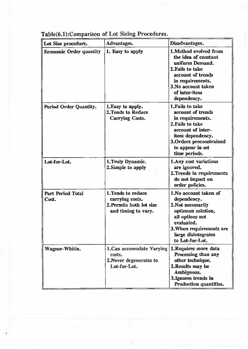
Table(6.1):Comparison of Lot Sizing Procedures.L o t S iz e p r o c e d u r e . A d v a n t a g e s . D is a d v a n t a g e s .

E c o n o m ic O r d e r q u a n t ity 1 . E a s y t o a p p ly 1 .M e t h o d e v o lv e d f r o m t h e id e a o f c o n s t a n t u n i f o r m D e m a n d .

2 .F a i l s t o t a k e a c c o u n t o f t r e n d s in r e q u ir e m e n t s .

3 .N o a c c o u n t t a k e n

o f in t e r - i t e m d e p e n d e n c y .

P e r io d O r d e r Q u a n t i ty . 1 .E a s y t o a p p ly .2 .T e n d s t o R e d u c e

C a r r y in g C o s t s .

1 .F a i l s t o t a k e a c c o u n t o f t r e n d s in r e q u ir e m e n t s .

2 .F a i l s t o t a k e a c c o u n t o f in t e r - i t e m d e p e n d e n c y .

3 ,O r d e r s p r e c o n s t r a in e d t o a p p e a r in s e t t im e p e r io d s .

L o t - f o r - L o t . 1 . T r u ly D y n a m ic . 2 .S im p le t o a p p ly

1 .A n y c o s t v a r ia t io n s a r e ig n o r e d .

2. T r e n d s in r e q u ir e m e n t s d o n o t im p a c t o n o r d e r p o l ic ie s .

P a r t P e r io d T o ta l C o s t .

1 .T e n d s t o r e d u c e c a r r y in g c o s t s .

2. P e r m it s b o t h lo t s iz e a n d t im in g t o v a r y .

1 .N o a c c o u n t t a k e n o f d e p e n d e n c y .

2 .N o t n e c e s s a r i ly o p t im u m s o lu t io n , a l l o p t io n s n o t e v a lu a t e d .

3 . W h e n r e q u ir e m e n t s a r e la r g e d is in t e g r a t e st o L o t - f o r - L o t .

W a g n e r - W h it in . 1 .C a n a c c o m o d a t e V a r y in g c o s t s .

2 .N e v e r d e g e n e r a t e s to L o t - f o r - L o t .

1 .R e q u ir e s m o r e d a ta P r o c e s s in g t h a n a n y

o t h e r t e c h n iq u e .2. R e s u lt s m a y b e

A m b ig u o u s .3 . I g n o r e s t r e n d s in

P r o d u c t io n q u a n t i t ie s .

When applying lot sizing methods a distinction must be made between, manufactured

and ordered parts. Price discounts can serve to complicate the situation.

6 . 2 . 2 L o t S iz e D e c is io n P o lic ie s

The Lot-For-Lot method of lot sizing is the most direct method available today.

Generated requirements are translated into order quantities without recourse to any

calculations to . economically "improve" the lot size. This rather simple method

however, has a number of inherent problems. Firstly, if costs were to vary across

the planning horizon, no account would be taken of this variation, and opportunities

to produce more cheaply would be missed. The number of actual orders generated

equals exactly the number of periods in which requirements were generated possibly

resulting in a large number of orders, of varying sizes at quite frequent intervals.

Often requirements are generated in quantities which the supplier cannot supply. This

may arise in cases where containers, or weight measurements are used to supply

materials. Generating requirements at this stage, without performing some Lot sizing.

procedure would cause immediate problems. Some lot sizing procedures have the

ability to compensate for trends in requirements, adopting suitable ordering policies,

dependant upon the variation of magnitude of requirements. The Lot-For-Lot

method, by ordering exact requirements generated, fails to do this.

E c o n o m ic O r d e r Q u a lity

One of the first lot sizing policies to be introduced was the economic batch size

policy. It is also one of the more widely used and accepted methods. The equation

below describes the technique.

EO Q = \2 x P x D

HC( 6 . 1 )

P: Order Costs.D: Average Period Demand.HC: Holding Cost.

An average demand is calculated over the span of the horizon, and an attempt is then

made to mimise costs by combining requirements. A static Lot size is determined,

and a number of periods demand can then be met from the produced lot. If however

requirements within the planning horizon are quite varied, some single period

requirements may be greater than the lot size, and an order decision policy must be

made based upon two alternatives.

1. Multiples of the economic batch size may be ordered.

2. The economic lot size may disintegrate to Lot-For-Lot.

If the first alternative is adopted, actual production may increase way beyond

requirements, the second alternative compounds any adverse effects due to employing

the EOQ policy by simultaneously operating a Lot-For-Lot policy.

P eriod O rd er Q u an tity

This method is a variation of the fixed order period method. It demonstrates an

attempt to keep inventory carrying costs at a minimum. An economic time interval

is calculated, based upon average, demand and economic order quantity, - attempting

to spread the batch size over a number of periods.

E con om ic T im e In terva l = E conom ic B atch S izeA verage D em and (6.2)

The procedure, then calls for ordering exact requirements over the interval. Carrying

costs figures may therefore be improved assuming fairly uniform demand, but large

variations in demand may continue to incurr high carrying costs. The method has a

number of similarities, to the pervious method in that any trends in requirements are

totally ignored, and no account is taken of the dependency between items. Unlike the

EOQ method however, orders are constrained to appear in preset time periods a set

number of periods apart, thereby preventing any capitalization on cost variations in

differing periods.

P a r t P e r io d B a la n c in g

This method also stems from the economic order quantity. It represents an attempt

to equate set up costs with the cost of carrying inventory. All information provided

by the requirements schedule is used. This required that the carrying cost involved,

when placing an order in period T for a period span of T + N must approximate the

cost of placing that order.

Examining the alternatives.

A. Place an order, in period T for period T,S requirements along:HC X [Vi(Ra)] = HC1 (6.3)

B. Place an order in period T for period T, and T + l requirements aloneHC X ['A(RJ + 3/2 (Rjt+1)] = HC1 (6.4)

C. Place an order in period T for periods T, T + l , T + 2 T + N requirements.HC X ^ (R * ) + 3/2 (Rit+1) ... ((2N-l)/2) (R,t+N)] = HC1 (6.5)

Where HC: Holding cost/period; HC1 total holding cost, R,t; Requirements, item

i period t.

When the holding costs, that would be incurred by placing an order in period T, to

cover the demand for N periods, approximates the order costs incurred, the lot size

is chosen to cover all previous requirements.

T h e L e a s t U n it C o s t (L U C )

This lot size model is based upon order and inventory costs. It may also

accommodate price break decisions. Requirements are accumulated over time

periods, and the total cost associated with placing the order in an earlier period

evaluated, until, the price per unit begins to increase. The policy which results in the

smallest cost per unit is then chosen.

Examinging the alternatives.

A. Placing an order in period T, to.cover the requirements in period T alone.

Total Cost Per Unit = [(Rit) x PP + SU]/(Rlt) (6.6)

B. Placing an order in period T to cover req. in period T, T + l

Total Cost Per Unit = [HC x (Rh+i) + (R* + Ru+i) x PP + SU]/(Rît Ru + i) (6.7)

C. Placing an order in period T to cover req. in Period T, T + l T + N

Total Cost Per Unit = [(HC x (R* + 1) + HC2 x (Rh+i) ...

Where PP: Production costs; SU: set-Up Costs.

If order policy C results in the lowest unit costs, it is then chosen to cover

requirements in period T to T + N , and the order is placed in period T. The next

order will then be placed in period T + N + l .

Least Period Cost (LPC)

Same method as that of least unit cost, except that the criteria for chosing the lot size

is changed. Least period cost (LPC) uses the lowest cost per period, rather than per

unit to determine the lot size. Once the various policies have been evaluated, the

policy which incurrs the least average period cost is chosen, to cover N periods. The

next order will then be placed in period T + N + l.

6.3.1 IntroductionBased upon the work of Zahorik et al [15], Billington et al [16], who developed linear

programming formulations for the series system in parallel, and general assembly case

respectively. The following three dimensional material requirement planning lot size

model has been developed.

•it+1

(6 .8)

6.3 MATERIAL REQUIREMENT PLANNING MODEL

The model seeks to minimize total costs, accumulated during production. These

costs, are made up of both production and holding costs. Set-up costs are completely

ignored by the model for two reasons.

1. They are assumed to be relatively small in comparison to production

costs.

2. As companies become more aware of Just-In-Time (JIT) techniques,

the emphasis will be on the further reduction of these costs.

The model allows costs to vary from period to period and in do doing account for

eventualities, such as overtime/undertime, variations in skill levels etc. Costs are

assumed to be linear.

External demand is assumed to be deterministic, and to occur, for each product at the

end item level. The span of the time periods, and their individual length (time) will

be as specified in the master production schedule (MPS), and will therefore be finite.

No backlogging of orders will be allowed. This requires that production in any

period, may be to satisfy demands made in future periods, but not those made in

previous periods. This requirement is in keeping with the master production

schedule, (MPS), which sets out demand figures from the present time to some

specific time in the future. If backorders were required, it would be up to the master

scheduler to accommodate them within the confines of the M PS.

The model itself, will have three subscripts, the first used to indicate the product, the

second the level at which the item occurs, and the last relating to the time period.

Final products, (i = 1..N) will occur at level j = 1, in all (or none), time periods.

The suffix j is also a level index, but is used to represent parent items, ie. items on

levels higher than the one in question.

Production is not assumed to occur instantaneously, production lead times are

included in the model. Production of any parent item, due to be completed, in a time

period t, with a lead time L, requires that component items are ready in a time period

T-L, in order that assembly be completed on time.

The general form of the MRP product structure depicts items with both multiple

parents (ascendants) and multiple descendants. Multiple descendants can be dealt

with, in the conservation of flow matrix, the difficulty arises in dealing with multiple

parents.

6 .3 .2 S t a t e m e n t O f A s s u m p t io n s

5 1. Deterministic External Demand.

2. Finite Planning Horizon.

3. No Backlogging Of Orders.

4. No Set Up Costs.

5. Linear Production Costs.

6. Constant Production Lead Times.

7. Any Item can have no more than on Parent (only on descendant).

8. Each product (k) must go through a similar sequence of events.

6 .3 .3 N o m e n c la tu r e

1. Subscripts

k = 1....M Product Index

i = 1 ....N Component Item Index

t = 1 ....T Planning Periods

j(i) = 2 ....N Parent Item Index

2. Constants

Cm Unit cost of production, product k, item i, period t.

Hut Unit cost of holding inventory item i, product k, periodt.

Dfcj External demand, product k, item j, period t.

L ^ Production lead time for item i, in product k.

3. . Decision Variables

I^t Inventory at the beginning of the time period. Byvirtue of the fact that no events can occur in between time periods, this inventory is equivalent to that available at the end fo the previous period.

Put The production of product k, item i, which becomesavailable, at the beginning o f period t.

D ^ The external market demand of product k, item i, inperiod t.

6 . 3 . 4 M o d e l F o r m u la t io n

1. Minimise

5 3 ^ki t Pki t + Hki t Ik i t ( 6 . 9 )kit kit

2. Subject To

^kit-1 ~ I k i t + ^kit ~ E ^i^kj (i) t*Lk(:ju)) ~ ^kit ( 6 . 1 0 )

6 . 3 . 5 D is c u s s io n O f T e n u s

Equation (6.9) states the objective of the model formulation which is to minimize the

production costs, for every product, at each and every item level, and in every

period. Holding costs incurred, during the same time periods must also be

minimised.

Equation (6.10) is termed the flow conservation matrix, and governs the flow, of

material from one production stage to the next. Consider product k, item i, in period

t. The first term of the equation relates to inventory held, for item i at the beginning

of period t. (lut.,).

The second term represents inventory left at the end of period t. This inventory is

obviously going to be the net of the initial inventory and any events or actions which

take place during that time period and have an effect on the inventory on hand figure

(Ikit). These events, are summarised by the next three terms.

The third term relates to production of product k, item i, period t which is due for

completion at the beginning of period t. This production will serve to increase the

on hand quantity ( P ^ .

The forth term relates to internal demand - demand which has been derived from

internal dependencies between items. M;, refers to the quantity of item i, required

per the production of one unit of the parent item j(i). If the production of one unit

is going to become available at the beginning of period t + L G(0), where refers

to the lead time of assembly of the parent item, then the quantity of item i, must be

removed from inventory, during period t. This serves to reduce the on-hand amount

held in inventory. (E M; Pkj(i)t+L(j(0))

The final term, refers to external demand. External demand, demand from the

market, is satisfied instantaneously, if no time lag occurs between the requirement,

and fulfillment, both happen within the same time period. (D^t)

6 . 3 . 6 M o d e l R e p r e s e n t a t io n

The model can be represented in terms of a three dimensional matrix structure as

follows:

1. Each'individual product is represented, successively parallel to the

page (k = 1..M)

2. Time Periods (t = 1..T), runs down the page, in successive sections,

each section corresponding to an item, in the product structure, giving

T x N Rows.

3. The inventory held and production carried out in the various time

periods, for each item, are represented, by the columns, advancing

across the page. This results in 2 x T x N columns. In total therefore

we have a three dimensional matrix, with, M x TN x 2 TN Entries.

NOTE the j axis, or columns also represents the various levels within the product

structure, dependent upon the number of items within each level.

6 . 3 . 7 I n t r o d u c in g T tem P la n n in g H o r iz o n s

Although the number of columns in the matrix is generally defined to be 2 x T x M

this number can be reduced by introducing the idea of a production horizon for each

and every item, within the product structure. This is done by letting the production

horizon for the product k, item 1, (ie. top level item) equal to the span of the

planning horizon as specified in the master production schedule.

Ri = T (6.11)

The production horizon for all items at lower levels are then determined alternatively,

using both the production horizon and lead time for assembly of parent items.

Rki = Rtj(i) - Lkj(i) i = 2 — N (6.12)

No production can take place, after and this ensures that all items produced, will

be done so in a time period which allows their inclusion in a proceeding sub-

assembly.

In keeping with this idea of timing, no production is allowed to appear in a given

period until, a number of time periods, equal to the lead time of that item has passed.

Pk* = 0, k = 1..M, i = 1..N, t = 1..L*

No initial inventories are allowed, at any stage of the production process, and once

the duration of the planning horizon has been completed, inventories cannot be held

into the next time period as they cannot be used in further sub-assemblies (t J> RJ.

Ifcio = 0

= 0, k = 1..M i = 1...N , t _> R,.

This leaves the .model, with the following qualifying constraints.

1. Put = 0, k = 1..M, i = 1...N , t = 1...L*

2 . Iuo = 0

3. Kut = 0 k = i = 1...N t > .R i

6 .3 . 8 F in a l M o d e l

The model becomes

1. Minimise

£ ^k it ?k it + Hkit I klt ( 6 . 1 3 )kit kit

Subject To

Xkit-i ~ ^ k it + Pitie_£ (Mi PkjU)t*LktJU))) =Dkit ( 6 . 1 4 )

k = 1..M , i = 1..N t = l...R u

Put = 0 k = 1..M, i = 1..N, t = l..L u

Ik io = 0

Iut = 0 k = 1-..M, i= 1..N, t>_ Ru

6.3.9 The M odel And Networks

A generalised network is a type of linear programming problem, and therefore can

be solved using any standard linear programming solution technique. The primary

reasons for adopting network formulations are.

1. The superior efficiency of generalised network codes.

2. The pictorial presentation, is a useful explanatory device.

In terms of matrix representation a generalized network may contain at most two non

zero elements, per column, ignoring the upper bound constraints. When these non

n-7

zero elements correspond to +. 1, the network is termed a pure network, examples

include, transshipment, transportation, assignment problems. If the generalised

network structure is not immediately apparent sets of linear transformations may be

employed to produce it.

The one dimension counterpart of the model matrix formulation is not itself a

network, however, it may possibly be solved using, decomposition technique, or as

a network formulation with side constraints. Advances in parallel processing will aid

the solution of the 3-D model.

6 3 . 1 0 M o d e l S im p li f ic a t io n s

At the present time, the model described in the previous section is difficult to solve.

The reasons for this fall into two main sections, firstly those pertaining to computer

processing capability, and secondly, those pertaining to mathematical programming

capability.

M athematical Programming

Linear programming methods in use today are very time consuming, especially when

branch and bound methods are used to solve integer linear problems. Because of this,

various other solution methods are being sought. Attention has been focused on

developing generalised network codes, to solve the linear programming problem.

When the model described in the previous section, is restricted to be 1 in the k axis,

(ie. 1 product), the matrix, when considered in its complete form, does not exhibit

network properties, firstly because some components have common parents, and

secondly because, parent items may require more than one component.

Decomposition methods, - which allow the determination of the optimal solution, by

first decomposing the problem into smaller sub problems, and then solving the

subproblems almost independently, may possibly be used to exploit the definite block

structure of the problem, in conjunction with network solutions.

At the present time however network solutions only apply to single parent single

component problem (ie. series case). To solve, the general assembly case, linear

programming methods, such as the simplex, or Big-M technique must be used.

C o m p u te r P r o c e s s in g

The computer processing capability required to solve the multi product case, would

be large, and very time consuming. This is because present day computers only have

one processor - The central processing unit - single processors are suited to solving

the single product case for up to 1000 components, assuming the matrix is

triangularised (Ho et A1 [17]). Investigation into the use of computers in parallel and

therefore, parallel processing which allows data to be input and manipulated very

quickly is ongoing. Use of minicomputers having 2N parallel processors are

becoming increasingly cost effective (N = 6-8). The problem associated with the

amount of data to be manipulated can best be seen by example. If a particular

company has a product range of 100 items, each with 100 components, and operates

from a planning horizon of 10 periods, then the no of constraints or equations to be

considered would be

10 x 100 x 100 = 100,000 constraints period product items

and

2 x 10 x 100 x 100 = 200,000 variables,

assuming production and inventory decision variables for each item.'

Attempting to solve problems of this size, on todays computers is impossible.

Model Simplifications

In order to investigate the model presented, the following modifications will be made.

1. Only one product will be considered.

2. The product, may only have components, on up to 5 levels.

3. The lead time for individual production processes is restricted to 1.

129

4. In order that the actual optimization ability of the solution technique

can be appreciated production costs will vary both per item, and across

the planning horizon.

5. Inventory holding costs will vary per item but no across the planning

horizon.

6. Demand patterns will be constrained to occur in 6 different ways.

A) Level B) Lumpy C) Increasing D) Decreasing E) Concave F)

Convex.

7. The product may have up to 8 components spread over the 5 levels.

8. The model will be investigated over a planning horizon of 6 or 12

periods. (Max cumulative lead time of product is 5).

9. Each item may only have one parent.

Minimise

- S ° U P i t + S H±t T i t ( 6 . 1 5 )t - i t - i

Subject To

^ ic - i - ^ it + Pic - i <6 - 1 6 >

1. i = 1..5, t = 1...12.

2. Pi» = 0 i = 1..5, t = 1.

3. Ik, = 0

4. Kft = 0, i = 1..5, t > .R i

NOTE Rl = 5

Ri = Rj(i) - Lj(i) Planning Horizon

Ri = Rjffi-i

6.4 SOLUTION METHODS

6 .4 .1 L in e a r P r o g r a m m in g (L P )

1

I n t r o d u c t io n

In its standard form, the linear programming form of a mathematical model consists

of an objective function, which must be maximised, (or minimised) and a number of

constraint equations, each with non-negative Righ Hand Sides (RHS). All equations,

in the model must be linear, which requires that:

1. The contribution of any variable in the objective function be directly

i proportional to that variable valve, ie. price breaks, discounts etc., do

not belong to the LP class of problem.

2. The objective function be the direct sum of individual contributions of

the different variables.

When all the constraint equations are plotted graphically, the area bounded by the

equations is referred to as the feasible solution space. Each point on or within the

boundary to the solution space, satisfies all the constraints, and represents a feasible

solution. The optimum solution however, can be determined by observing the

direction which maximizes (or minimizes) the objective function, if the line

representing the objective function is moved in this direction, along a line 90° to it,

until any further motion renders the objective function line outside the feasible region,

then the optimun value of the objective function has been found. The values of the

variables required, to give this optimum solution are then found by solving

simulataneously the constraint equations which intersect at this optimum point.

6 . 4 . 2 S im p le x M e t h o d /A lg o r i t h m

A distinction must be made between the simplex algorithm, and the simplex method.

The simplex algorithm describes the actual solution method whereas the method

encompasses both the method and the transformation from the initial linear

programming model, with enequality constraints to the format required by the simplex

algorithm.

If a constraint is of the form (< ) . then in order to make the LHS equal the RHS a

certain slack variable S, must be added to the LHS. Alternatively, if the constraint

is of the form ( > ) then a slack variable must be subtracted from the LHS. All the

slacks must also be constrained to be non negative. Once all the inequalities have

been reduced to equalities, the model is in the form required by the simplex

algorithm.

The algorithm is an iterative procedure, which starts at a feasible comer point, and

systematically moves to the next adjacent comer point, until the optimum point is

reached. The only rules required are:

1. Must move to an adjacent solution space.

2. You cannot regress.

The simplex method deals only with points on the boundary, called extreme points

because the optimal solution will always be on the boundary. At every extreme

comer point, two types of variables exist.

1. Non basic variables.

2. Basic variables.

Non basic or zero variables, are those variables which do not appear in the solution

at that point. Adjacent extreme points differ by only one variable, in time basic (non

zero) solution set. The variable which enters the basic solution, is called the entering

variable, and the variable which leaves the basic solution to join the set of non basic

variables is called the leaving variable. The choice o f entering and leaving variable

is an integral part of the simplex algorithm. The entering variable is usually that

variable, which by increasing its value above the zero level, will achieve the greatest

increase in objective function value, at the next iteration. Conversely leaving

variables are chosen because, when, the entering variable reaches its maximum value,

at the adjacent extreme point, the leaving variable will be the first to reach zero.

6 .4 .3 M e t h o d o f P e n a lty

The method of penalty technique, refers to the actual setting up of the problem LP,

so that it can be solved by the simplex algorithm. The simplex algorithm always

assumes, a starting basic solution, (usually equivalent to the slack variables).

However, if one or more of the constraints are not inequality constraints, then, the

number of slacks, will not equal the number of equations and it is difficult to decide,

what variables should be set to zero. The method of penalties introduces the idea of

artificial variables.

When all inequalties have been removed artificial variables Ri are added to the LHS

of any equations which do not have any slack variables. By assigning these variables

very small (maximise) or very large (minimize) positive coefficients in the objective

function they will eventually be forced to zero. The starting feasible basic solution

will then consist of any slack variables plus any artificial variables, and the non basic

variables, of surplus and expected final solution basic variables. The simplex

algorithm can therefore complete normally. Note, the Linprog 2 package referred to

in this chapter, uses the penalty method, to set up the relevant LP.

6 .4 .4 B r a n c h a n d B o u n d M e t h o d

Branch and Bound Methods apply to both pure (all variables non-negative) and mixed

(some variables non-negative) problems. The general idea behind the method is to

firstly solve the program as an LP and then restrain any non integer values to be

integers, and solve the resultant LP’s. If Xr is found to be non integer, restraining

Xr, over the interval

[X J <. Xr <. [X,.+1], (6.17)

Results in two subproblems. By enforcing integrality, the branching strategy reduces

the size of the feasible solution space. Each problem can then be solved as an LP

using the same objective function. If the solution is found to be feasible, and integer,

and the value of the objective function smaller than any previous value, the solution

is accepted as the best available bound. Any branching which results in a non­

integer, solution, and has an objective function value less than the best bound, is not

branched from again.

6 .4 .5 I n t r o d u c in g I n v e n t o r y T o T h e M o d e l

The model as stated in the previous chapter is not complete. No inventory has been

introduced to the model, and therefore none will reach the various demand nodes,

when the model is input to the computer. Two methods exist whereby inventory can

be introduced.

The first entails accumulating all end item demand across the span of the planning

horizon, and letting the sum of the production at the end item facility equal to this

accumulated production. The equation below summarizes this technique (i = l).

T TE Pit = E DEMlt (6.18)

t = l t = l

This allows the model to work out the cheapest production pattern at end item level

before proceeding further.

The second method requires the introduction of initial inventory to the model in time

period zero. This initial inventory must be greater than or equal to the accumulated

demand across the span of the planning horizon at end item level. This is

summarized by the equation.

TI10 = E DEM* (6.19)

t = lIf the initial inventory requirements are not sufficient to satisfy demand, the model

will not run successfully. Table (6.3) compares the relative merits of both

techniques, for a three facility assembly model, with varying production costs and

constant holding costs. Table (6.4) defines the cost structure for the model.

TABLE (6.2): Comparison of both methods of Inventory Introduction

No of Iterations Solution Time (Sec) Obj. Function

M ETHOD 1 22 A 80

M ETHOD 2 25 .45 80

The first method has advantages when dealing with the development of an MRP II

type model, because the equation (6.18) can be used to constrain production at

individual facilities to a number of planning periods and so introduce a capacity

13d

• • •

I 1 I

1 2 3Time Periods.

Network Diagram (a)

A

Product Structure, (b)

Fig(6.3)

A Demand Level

Product Structure.

Fig (6.2)

TABLE (6.4): Variables for Model described in Fig. (6.2)

PlanningPeriod

1 2 3 4

Dem.P attern

1 1 1 1

P COSTS Item A, B 4 3 2 1

H Costs Item A, B

2 2 2 2

TABLE (6.3): Production and Holding Cost Pattern For A 3 FacilityModel

PlanningPeriod

1 ' 2 3 4 5 6

(ITEM 1) PCOSTS

12 10 8 6 4 2

(ITEM 2) PCOSTS

10 5 1 1 5 10

(ITEM 3) PCOSTS

1 5 10 10 5 1

(ITEM 1) HCOSTS

2 2 2 2 2 2

(ITEM 2) HCOSTS

1 1 1 1 1JL 1A

(ITEM 3) HCOSTS

1 1 1 i 1 1

(ITEM 1) DEM

1 1 1 1 1 1

P COSTS: Production Costs

H COSTS: Holding Costs

DEM: Demand Pattern

planning dimension to the model.

6.4.6 I^ot Sizing, and Modelling

Imagine a product structure of the type Fig. (6.2) manufactured over a planning

period, of length four periods. The demand pattern, production costs and holding

costs, are specified in Table (6.4).

The resultant constraint equations will then be defined in Eqns. (6.20 - 6.27).

- I a i + P ai = 1 (Prod. A Period 1) (6.20)

■ Ia 2 "1“ P a2 = 1 (Prod. A Period 2) (6.21)

" A2 P a 3 = 1 (Prod. A Period 3) (6.22)

“ Ia4 "I" P a4 = 1 (Prod. A Period 4) (6.23)

“ bi + P bi " P ai = 0 (Prod. B Period 1) (6.24)

- IB2 + PB2 - P A2 = 0 (Prod. B Period 2) (6.25)

■ ÏB3 + P b2 " P a 2 = 0 (Prod. B Period 3) (6.26)

- I b4 + P b4 - P A4 = 0 (Prod. B Period 4) (6.27)

No initial inventories are allowed, which required that IA0, Iso are set to 0. If

inventories were left over at the end of the planning horizon, additional holding costs

would be incurred, and I^ IA4 are also set ot zero.

There must however be some starting point, from which the program run originates,

and because, it is the production lot sizes that interests us, an additional constraint,

must be added, that specifies, the cumulative production requirements of the end

product. (See Sect. 6.4.2).

Pai + Pa2 + Pa3 + Pa4 = 4 (6.28)

Using the production and holding costs for item A, as specified in the objective

function, the package chooses the cheapest production plan. (Note the model has

been established in such a way as to avoid back logging only forward production is

allowed). The following alternatives would be considered, and one accepted.

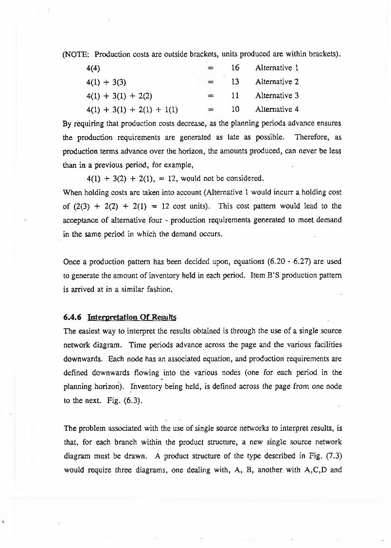
(NOTE: Production costs are outside brackets, units produced are within brackets).

By requiring that production costs decrease, as the planning periods advance ensures

the- production requirements are generated as late as possible. Therefore, as

production terms advance over the horizon, the amounts produced, can never be less

than in a previous period, for example,

4(1) + 3(2) + 2(1), = 12, would not be considered.

When holding costs are taken into account (Alternative 1 would incurr a holding cost

of (2(3) + 2(2) + 2(1) = 12 cost units). This cost pattern would lead to the

acceptance of alternative four - production requirements generated to meet demand

in the same period in which the demand occurs.

Once a production pattern has been decided upon, equations (6.20 - 6.27) are used

to generate the amount of inventory held in each period. Item B’S production pattern

is arrived at in a similar fashion.

6.4.6 In terp reta tion O f Results

The easiest way to interpret the results obtained is through the use of a single source

network diagram. Time periods advance across the page and the various facilities

downwards. Each node has an associated equation, and production requirements are

defined downwards flowing into the various nodes (one for each period in the

planning horizon). Inventory being held, is defined across the page from one node

to the next. Fig. (6.3).

The problem associated with the use of single source networks to interpret results, is

that, for each branch within the product structure, a new single source network

diagram must be drawn. A product structure of the type described in Fig. (7.3)

would require three diagrams, one dealing with, A, B, another, with A,C,D and

4(4)

4(1) + 3(3)

4(1) + 3(1) + 2(2)

4(1) + 3(1) + 2(1) + 1(1)

16 Alternative 1

13 Alternative 2

11 Alternative 3

10 Alternative 4

finally one dealing with A ,C,E,F. This leads to much duplication of data.

6.4.7 Inclusion of Varying Planning Horizon

Again looking a the product structure in Fig. (6.2) assuming that the results obtained

are going to be offset to include manufacturing lead times, then production of item

B, should be stopped in a time period T ^ - Lead time of A, anything produced in

periods later than this can not be used in useful production of A. This results in a

sort of rolling planning horizon.

Item A - Produced in four periods.

Item B - Produced in three periods.

Also connected with the idea of planning horizon, is that of final inventory. If the

inventory, at the end of each planning horizon is not set to zero, then the possibility

of being left with unused inventory arises. If both IB3> and P ^ are set to zero, then

inventory items have no way of being produced at PA4 and. the only way of satisfying

demand is to produce at facility A, in period 3, and hold the item to satisy period

four demand until period four. If it is cheaper to hold item, B than item A, then

setting Ig3 to zero is not the correct solution.

Examining the Eqn. (6.28), (ie. time period 4) for item B. It consists of items, which

are known already and/or are set to zero, it can therefore be completed removed from

the nodel. For any model therefore, as you advance down item level the no of

equations can be reduced by the item level number less one.

6.4.8 Specific Models

This section slowly develops simple but specific models from the more general model

discussed in section 3.

Each model is examined assuming a uniform market demand of four units spread

equally over four periods. The inclusion of lead times however extends the planning

horizon by an amount equal to the cumulative lead time of the product. Each model

is discussed individually in relation to the following:

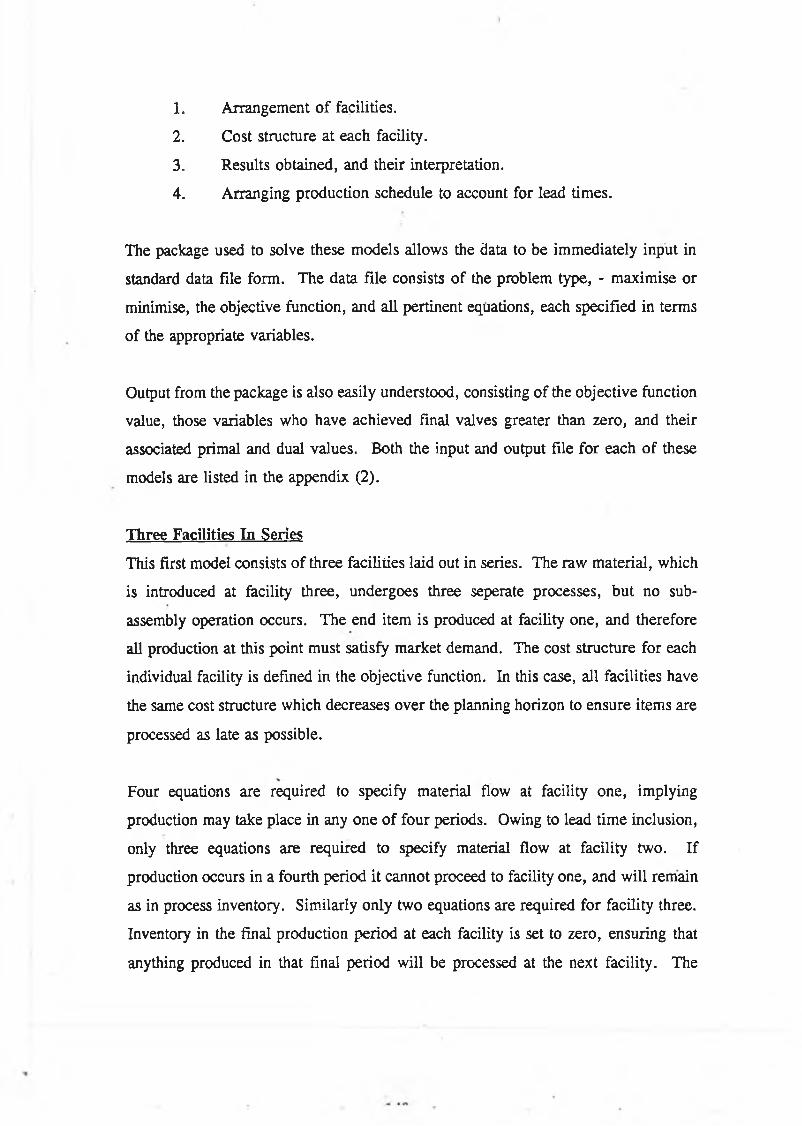
1. Arrangement of facilities.

2. Cost structure at each facility.

3. Results obtained, and their interpretation.

4. Arranging production schedule to account for lead times.

The package used to solve these models allows the data to be immediately input in

standard data file form. The data file consists of the problem type, - maximise or

minimise, the objective function, and all pertinent equations, each specified in terms

of the appropriate variables.

Output from the package is also easily understood, consisting of the objective function

value, those variables who have achieved final valves greater than zero, and their

associated primal and dual values. Both the input and output file for each of these

models are listed in the appendix (2).

Three Facilities In Series

This first model consists of three facilities laid out in series. The raw material, which

is introduced at facility three, undergoes three seperate processes, but no sub-

assembly operation occurs. The end item is produced at facility one, and therefore

all production at this point must satisfy market demand. The cost structure for each

individual facility is defined in the objective function. In this case, all facilities have

the same cost structure which decreases over the planning horizon to ensure items are

processed as late as possible.

Four equations are required to specify material flow at facility one, implying

production may take place in any one of four periods. Owing to lead time inclusion,

only three equations are required to specify material flow at facility two. If

production occurs in a fourth period it cannot proceed to facility one, and will remain

as in process inventory. Similarly only two equations are required for facility three.

Inventory in the final production period at each facility is set to zero, ensuring that

anything produced in that final period will be processed at the next facility. The

Faci

litie

s.

Time Periods.

| i ,1 j , j-

Oem.

rl

n

N etw ork D iagram . Fig.(6.5b) P ro d u c t S tru c tu re . F ig .(6 .5a)

Facility 2

Facility 1

! 3 2• -- ■■ #

r i1 i1 i1

s2Time Periods. N etw ork D iagram . Fig.(6.6b). P roduct S tru c tu re F ig .(6 .6a)

model is represented graphically in Fig. (6.5a). A network interpretation of the

solution is shown in Fig. (6.5b).

At the final facility, facility one, demand is specified as being uniform, with a

magnitude of one in each period. The model specifies however, that any units

processed, in the final production period in the preceding facility, must not be

allowed to accumulate, in a suceeding period, the final production period, at facility

one is period 3, and inventory must be carried over to meet the demand in period

four. A similar situation arises when inventory is transferred between facility three

and facility. Setting the various inventory to zero, thereby introduces a method of

controlling the periods in which production takes place.

From Fig. (6.5b), it is obvious that production occurs three times at facility one and

twice in both of the other facilities. Incorporating a lead time of one of each facility

one to three means that firstly end items will not be available to the end of the time

period in which they appear. Secondly facility two items, - in order to be ready for

processsing at facility one in the specified time period, - must be processed in an

earlier period. Facility’s three production must be similarly offset resulting in the

following complete production plan.

TABLE (6.5): Results Three Facilities In Series

Time Period 1 2 3 4 5 6

Production Facility 3 Item 3 1 3 0 0 0 0

Facility 2 Item 2 0 1 3 0 0 0

Facility 1 Item 1 0 0 1 1 2 0

Three Facilities General Assembly S tructure

This model again consists of three facilities, but instead of arranging the facilities in

series they are organized in an assembly format. Two different raw materials are

processed at level two, at facility two and three respectively and are then sub­

assembled together at facility one. Again the cost structure for each individual

facility is defined in the objective function. Cost structures at each facility, and each

period vary. (See Appendix ).

Four equations are used to define material flow at facility one. Facilites two and

three however, both appear at the same level within the product structure and will

therefore require three equations each, allowing production in three periods instead

of four. Inventory in the final production periods at each facility are constrained to

zero. Ensuring anything processed in the final production period, will be procesed

at the next facility. The model is represented graphically in Fig. (6.6a), and a

network interpretation of the solution is shown in Fig. (6.6b). As explained

previously, using a single source, network to interpret results, requires additional

diagrams for each branch of the product structure. By virtue of possessing two

branches, (1,2) and (1,3) this model requires two network diagrams to interpret

results.

For reasons explained in (6.4.1), inventory is carried from period 3, facility 1, to

meet demand in period four. Owing to the different cost structures, facility two’s

production pattern and facility three’s pattern will differ. Taking production and

holding costs into account, all the demand placed on facility two by facility one inthe

first period results in minimizing the cost for that facility. Inventory is then carried

to meet the demand at the varying production periods facility, ensuring material flow

constraints are satisfied at all times. Facility three’s cost structure results in the same

production pattern as that of facility one, ensuring the items produced at facility one,

are produced in the same quantities at facility two, and no items of inventory are

carried from a previous period.

Incorporating a lead time of one for each facility, necessitates an expanded planning

horizon. Facilities two and three will obviously begin production in the same time

period, because they appear at the same level within the product structure. If

however the lead time for production at facility two was twice as long as that at

facility three production would have to start in an earlier period.

TABLE (6.6): Results Three Facilities; Assembly Structure

Time Period 1 2 3 4 5 6

Production Facility 3 Item 3 0 0 1 1 2 0

Facility 2 Item 2 0 4 0 0 0 0

Facility 1 Item 1 0 1 1 2 0 0

Two Facilities In Series. - Two Products

This model demonstrates how■ the general model can incorporate separate

manufacturing processes. The first process consists of two facilities in series,

facilities four and three. End items are manufactured at facility three, and so demand

at that facility is specified by the market. Raw materials are introduced at facility

four. The manufacturing process described by facilities one and two operates in a

similar fashion with raw material being introduced at facility two, and end items

being completed at facility one.

The cost structure for each individual facility is defined in the objective function

(Appexdix 2). In this case facilities one, three and four have the same monotonically

decreasing production cost, item four can be produced very cheaply at period one,

at facility four, but production in future periods proves expensive.

3Time Periods.

■3,3U.

Time Periods.

Facility 31 1 2

I1 11 i j i

•

Facility 24

3 2 *

Facility 1 1 1 2

1

J1 I1 11 p

N etw ork D iagram . Fig.(6.7b)

Facility 2k \ u

• *

Facility 1 I 2

1

l i l1 h* *

Facility 3 6

H ! • • *

Facility 1 2

1

2

1

I1 I1 ji ji

N etw ork D iagram F ig .(6.8b)

(a)

I

2(b)

P ro d u c t S tru c tu re . Fig,(6.7a)

Oem..1

(3)

Product Structure. fig .(6.8a)

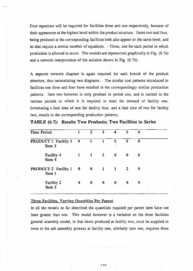
Four equations will be required for facilities three and one respectively, because of

their appearance at the highest level within the product structure. Items two and four,

being produced at the corresponding facilities both also appear on the same level, and

so also require a similar number of equations. - Three, one for each period in which

production is allowed to occur. The models are represented graphically in Fig. (6.7a)

and a network interpretation of the solution shown in Fig. (6.7b).

A separate network diagram is again required for each branch of the product

structure, thus necessitating two diagrams. The similar cost patterns introduced in

facilities one three and four have resulted in the correspondingly similar production

patterns. Item two however is only produed in period one, and is carried to the

various periods in which it is required to meet the demand of facility one.

Introducing a lead time of one for facility four, and a lead time of two for facility

two, results in the corresponding production patterns.

TABLE (6.7): Results Two Products; Two Facilities in Series

Time Period 1 2 ' 3 4 5 6

PRODUCT 1 Facility 3 Item 3

0 1 1 2 0 0

Facility 4 Item 4

1 1 2 0 0 0

PRODUCT 2 Facility 1 Item 1

0 0 1 1 2 0

Facility 2 Item 2

4 0 0 0 0 0

Three Facilities. Varying Q uantities Per Parent

In all the models so far described the quantities required per parent item have not

been greater than one. This model however is a variation on the three facilities

general assembly model, in that items produced at facility two, must be .supplied in

twos to the sub assembly process at facility one, similarly item one, requires three

I

units of item three produced at facility three. This increase in magnitude of quantity

required per parent is easily accomodated within the model, by multiplying the

corresponding term in the model by the required factor. Obviously an increase in the

number of units produced at each facility will also occur. In the models discussed,

market demand has been set at four units divided informly across the planning period,

dependant demand at facilities two and three will necessarily increase to eight and

twelve respectively.

The cost structure for each individual facility is defined in the objective function

(Appendix). Items one can be produced at facility one, very cheaply in periods one

and three. Items two can be produced very cheaply in periods one and three. Item

three’s production costs decrease monotonically across the spectrum of the planning

horizon. For reasons explained in previous sections item one’s production at facility

one is described by four equations, and items two and three are similarly described

by three equations. The model is represented graphically in Fig. (6.8a), and a

network interpretation of the solution shown in Fig. (6.8b).

The ability to produce cheaply in periods one and three as specified in the objective

at facility one, is evident from the network diagram, where all production at that

facility is constrained to appear in those periods. Production can take place very

cheaply in periods one and two, as demonstrated in the diagram. Total production

at this facility equals eight, -twice the production at facility one, and each individual

demand placed on facility two by facility one must be met in multiples of two.

Similarly, each individual demand placed on facility three by facility one must be met

in multiples of three. Item three could be produced more cheaply in period three,

however the net effect which would result in changing the overall production plant

to accomodate production in this period would not result in a decrease in costs, and

therefore is ignored. The offset of production plans at the respective facilities caused

by the introduction of lead times at each facility, results in the following production

plan.

147

TABLE (6.8): Results Three Facilities; Varying Quantity Per Parent

Time Period 1 2 3 4 5 6

Facility One Item One 0 0 2 0 2 0

Facility Two Item Two 0 4 4 0 0 0

Facility Three Item Three 0 6 0 6 0 0

Four Facilities. Varying Quantities Per Parent

This model requires four facilities to complete the manufacture of the product. Raw

materials are introduced at facility’s two and four and the end item becomes available

in facility one. Facility three, which occurs between facility one and four, processes

the inventory which arrives from item four, but no sub assembly takes place.

Quantities per parent item greater than one, are included in the model in the same

manner as before. The cost structure for each individual facility is defined in the

objective function (Appendix ). Each facility has the same cost structure, decreasing

monotonically over the planning horizon, however, as you go down the product

structure the number of periods available in which production can take place will

reduce.

Four equations specify facility one’s production. Three equations the production at

each facility in level two, and two equations,for facility’s four production. If the

number of levels withing the product structure was to increase past five levels then

the span of the planning horizon would have to be extended beyond the new

cumulative lead time of the product. The model is represented graphically in Fig.

(6.9a) and a network interpretation of the solution shown in Fig. (6.9b). Again

because the product structure has two branches, the network diagram falls into two

parts.

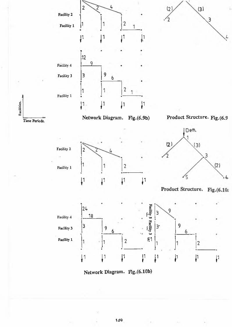
Faci

litie

s.

Time Periods.

Facility 4

Facility 3

Facility 1

Facility 2

Facility 1

Facility 4

Facility 3

Facility 1

j i j i ,1 j i

12

j1 J1 j! j1

N etw ork D iagram . Fig.(6.9b)

I1

P ro d u c t S tru c tu re . F ig. (6.9

18

F1

I1 I1 P i1 J1N etw ork D iagram . Fig.(6.10b)

I1 I1 I1

tdO

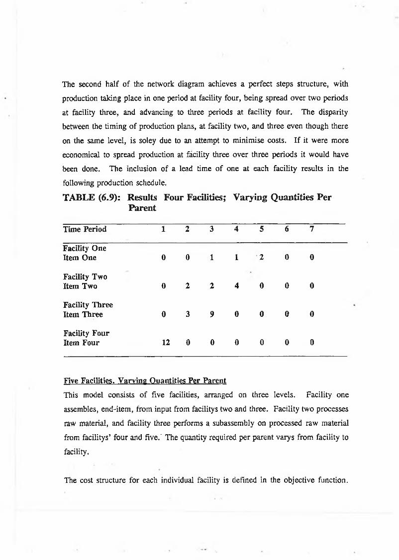
The second half of the network diagram achieves a perfect steps structure, with

production taking place in one period at facility four, being spread over two periods

at facility three, and advancing to three periods at facility four. The disparity

between the timing of production plans, at facility two, and three even though there

on the same level, is soley due to an attempt to minimise costs. If it were more

economical to spread production at facility three over three periods it would have

been done. The inclusion of a lead time of one at each facility results in the

following production schedule.

TABLE (6.9): Results Four Facilities; Varying Quantities Per Parent

Time Period 1 2 3 4 5 6 7

Facility One Item One 0 0 1 1 2 0 0

Facility Two Item Two 0 2 2 4 0 0 0

Facility Three Item Three 0 3 9 0 0 0 0

Facility Four Item Four 12 0 0 0 0 0 0

Five Facilities. Varying Quantities Per Parent

This model consists of five facilities, arranged on three levels. Facility one

assembles, end-item, from input from facilitys two and three. Facility two processes

raw material, and facility three performs a subassembly on processed raw material

from facilitys’ four and five.' The quantity required per parent varys from facility to

facility.

The cost structure for each individual facility is defined in the objective function.

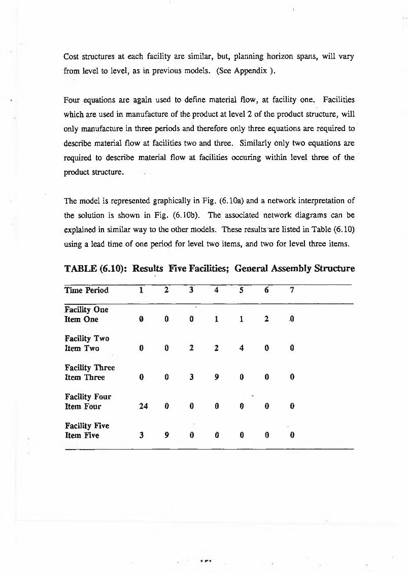
i

Cost structures at each facility are similar, but, planning horizon spans, will vary

from level to level, as in previous models. (See Appendix ).

Four equations are again used to defme material flow, at facility one. Facilities

which are used in manufacture of the product at level 2 of the product structure, will

only manufacture in three periods and therefore only three equations are required to

describe material flow at facilities two and three. Similarly only two equations are

required to describe material flow at facilities occuring within level three o f the

product structure.

The model is represented graphically in Fig. (6.10a) and a network interpretation of

the solution is shown in Fig. (6.10b). The associated network diagrams can be

explained in similar way to the other models. These results are listed in Table (6.10)

using a lead time of one period for level two items, and two for level three items.

TABLE (6.10): Results Five Facilities; General Assembly Structure

Time Period 1 2 3 4 5 6 7

Facility One Item One 0 0 0 1 1 2 .0

Facility Two Item Two 0 0 2 2 4 0 0

Facility Three Item Three 0 0 3 9 0 0 0

Facility Four Item Four 24 0 0 0 0 0 0

Facility Five Item Five 3 9 0 0 0 0 0

6.4.9 limitations Placed On Model By Linprg2 Package

The.Linprg2 package, used for the previous worked examples, is a very small

package, used only for demonstration and testing. The maximum number of

constraints that may be imposed is twenty and the total number of elements present

in the objective function may not exceed thirty.

Before examining the relationship between items, levels and planning horizon, it must

be pointed out, that, the minimum planning horizon required is independant of the

number of items within the product structure, but is dependant upon the number of

levels.

For a planning horizon of four periods and a manufacturing concern, with all facilities

arranged in series, Fig. (6.11), the no. of constraint equations generated is

4 + 3 + 2 + 1 = 10

At levels to 0-3 respectively. This means however that 10 of the 20 possible

constraints have not been used up, and only twenty elements appear in the objective

function. If one item, (also with a lead time of one) is added to the product structure

at level two and another at level three the number of constraint equations increases

to:

4 + 3 + 2 + 2 + 1 + 1 = 13,

And objective function elements to 26. Tables (6.11 - 6.13) describe the relationship

between items, levels and planning horizon, keeping in mind the constraints of the

Linprg2 package.

When an item is added to a product in an already existing level, the cumulative lead

time, will not change, and so neither therefore will the minimum planning horizon,

the minimum number of equations therefore, will only increase by a magnitude equal

to the cumulative lead time less the level to which the item has been added. The

maximum planning horizon, determines the number of equations which will be

generated and is therefore determined by the package size, which sets a limit on the

number of equations generated. As items within the product structure increase, the

Faci

litie

s.

4

Time Periods.

Facility 4

Facility 3

Facility 1

Facility 1

Facility 2

Facility 1

Facility 4

Facility 3

Facility 1

1

r

12

r r j1

1

r1 .

j i j i | i

N etw ork D iagram . Fig.(6.9b)

24

3

1

18

I1

P ro d u c t S tru c tu re . F ig .(6.9

jDem .

(3)

, L

P ro d u c t S tru c tu re . F ig .(6.10

?n'-ci/» I?

?n

i 1 i1 r p r

N etw ork D iagram . Fig.(6.10b)

i1 I1 I1

TABLE (6.11): Increasing Items, (Within Levels)

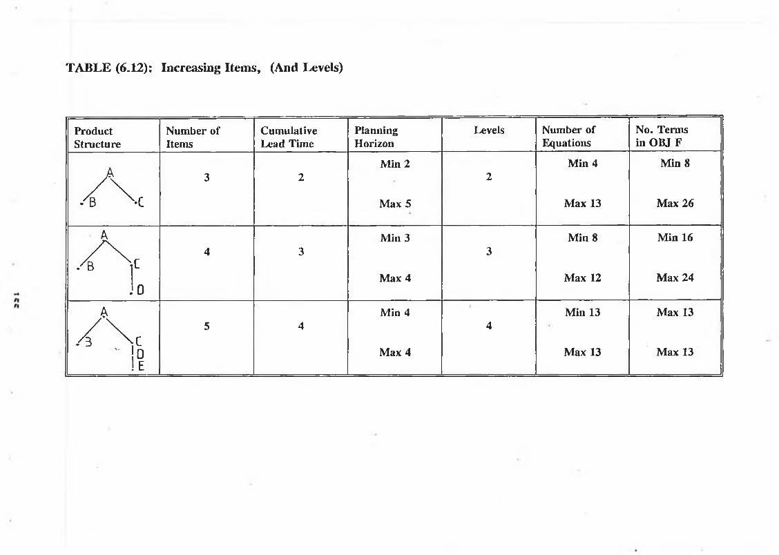
TABLE (6.12): Increasing Items, (And Levels)

ProductStructure

Num ber of Items

Cumulative Lead Time

PlanningHorizon

Levels Number of Equations

No. Terms in OBJ F

A c3 2

M in 2

Max 5

2M in 4

Max 13

Min 8

Max 26

A. 0

4 3Min 3

Max 4

3M in 8

Max 12

M in 16

M ax 24

A ci ï

5 4Min 4

Max 4

4Min 13

Max 13

Max 13

M ax 13

TABLE (6.13): Increasing Levels Only

ProductS tructure

Num ber of Items

Cumulative Lead Time

PlanningHorizon

Levels Number of Equations

No. Terms in OBJ F

0_C_B_A4 4

Min 4

Max 4

4Min 10

Max 10

Min 20

Max 20

A

.0

4 3M in 3

Max 4

3Min 8

Max 12

M in 16

Max 24

4 2Min 2

Max 4

21

M in 5

Max 13

M ax 10

Max 26

rroQucr :>rrucrures.Demand Leve l

Level 1

Leve l 2

(a)Level 3

Oi*-4

C

(b)

EV

Fig(6.12) Product Structure.

A*

Bm

.. C

.. Ü

(a)

A

Fig(6.11)

number of equations will increase, but the increase is determined, by the planning

horizon length, and also, the items position with the structure, Table (6.11).

When both the item and levels are increased simultaneously the cumulative lead time

must also increase, which means that the minimum planning horizon will also

increase. The maximum planning horizon will again eventually start to reduce, by

virtue of the constraint placed upon it by package size. The number of equations

generated, is dependant upon both the planning horizon length, and the distribution

of items, for example, moving an item from level to the next lower level reduces the

number of equations by one. Fig. (6.12) for planning horizon of four, has

4 + 3 + 3 + 2 + 2 = 14

Whereas Fig. (6.12b) generates

4 + 3 + 3 + 2 + 1 = 13

The planning horizon, always sets the starting number of equations, ie. at level 0, and

the number of equations at the other levels are determined accordingly. As the

number of items increase, the maximum cumulative lead time (CLT) will increase,

but, the minimum CLT will remain constant.

The relationship between items/levels/time periods, is ultimately a very simple one.

The number of items, which can be added to product structure, is determined by the

rate of convergence of the minimum to maximum planning horizons. By adding

items to the product structure within levels, with maximum planning horizon reduces,

converging towards the minimum planning horizon. When adding items to a product

structure and generating the item on a new level, both the minimum planning horizon

increase, and the maximum reduces. When the maximum planning horizon is

equivalent to the minimum value no more items may be added to the product

structure, unles the package capacity is increased. This will happen at a much slower

rate however when the items are added, to an existing level.

6.5 THE SCICON1C AND MGG PACKAGES

6.5.1 Explanation Of Relationship Between Input To Both Packages

The package used to investigate the examples in section 4.6 places limitations on the

size of the model (See Section 4.7.1). It was therefore decided that to test the model

performance under various operating conditions, a more advanced programming

package would be used. The best available package was SCICONIC, operating on

the University main frame, using a matrix generator to formulate the problem file.

Using the Linprg2 package, the model, was submitted (in equation form) in a data file

directly to the package (Appendix 2). Larger mathematical programming packages

used for problem solving throughout industry operate using input presented in what

is referred to as a standard matrix format. The formulation of this standard matrix

format is done by specifying, pertient data, in program form (Appendix 3a). This

data consists of any subscripts, external valve names, or equations used in the model

formulation. Actual data required by the model, (ie. holding/production costs) are

supplied in a separate data file (Appendix 3b) in a format specified by a spin off file

generated by this program. Once this has been created, the standard matrix format

can be generated (Appendix 3c).

In the model formulation file, each equation is given a name, whether it be the

objective function or a material balance constraint. The matrix file consists of three

sections. The first section lists the name of each individual equation. In order to

identify the various equations more easily. The objective function was named "cost".

Equation introducing capacity "CAP" with a number specifying facility, and any

material balance equations "MATB" proceeded by two numbers, one signifying

facility and a second the period in which it occurs. MATBB14, is therefore

concerned with material flow at facility one and period four.

1«0

Defines Facilities(i), Periods(t).

Defines Costs(C,H), Deman d(D), in terms

of Suffices.

Defines Variables(P,I) in Terms of Suffices.

Defines Objective Function.

Specifies Material Balance Constraints in terms of Variables

and Elements.

Defines and abbreviates Numerical Values in Alphabetical Form,

Signals end of Program.

Summary of Program File Sections. Fig.(6.13).

1 /TA

The second section consists of variable names, equation names and integers. Each

variable is listed once, and adjacent to it is the name of the equation it appears in, and

the associated integer value (multiple) it take on, in that equation. By listing each

variable and associated integer it is possible to compile the left hand side of any

equation, for example.

MATB21: -1(IN21) + 1 (PR21) -1 (PR11) = 0 (6.30)

The right hand side of the equation is zero, because section three only lists those

equations whose right hand sides have a value other than zero.

The above equation is comparable to any found as input to Linprg2 in Appendix (2).

The output from the sciconic package is Appendix (3d) is different to that of the

Linprg2 package. Output in the case consists of three sections. The first gives data

regarding number of iterations required, to arrive at the optimal solution, and the

name and valve of the objective function. The second section lists the various

equation names, and the corresponding righ hand side values. The upper and lower

bounds are also listed. These will vary only when branch and bound is used. Section

three lists all the variables used, and the valves they obtain in the optimal solution

input costs, - production and holding costs are also listed for each variable.

6.5.2 SCICONIC And Matrix Generation

Mathematical programming techniques are used in a wide variety of areas to generate

optimal solutions to problems. In order to solve the problem, the problem must be

formulated in a way that can be universally understood. This format is referred to

as a standard matrix (MPS) format. In order to generate this standard matrix format

one of two appraches may be adopted,

1. Write the matrix generater in standard programming language, ie

fortran.

1 ZT1

Matrix Generation Process. Fig(6.14)

2. Write the matrix generater program in a specialized high level

language.

MGG (Matrix generator, generator), is a high level mathematical programming

language which combines the advantages of both approaches.

6.5.3 FormulationA formulation is shown in Appendix (3a). The formulation consists of many sections,

namely:

1. Subscripts

2. External Values

3. Variables

4. Problem Specification

5. Constraints

6. Elements

7. . End.

The subscripts section is used to define, the various suffices used in the model and

their respective maximum values. The external values, is used to name, the various

constraints required in the model which must be read in from a data file. The

variables section, is used to define the variables, which must be calculated by the

program. The objective function, is defined in the problem section, in terms of the

variables and constants which have been defined. The constraints section, defines the

various constraints required. Notice that all the constraints must be named with

respect to the suffices used in the program. The elements section, is just used to

define any of the constraints, which have been given names interval to the generator,

generator file, such as the RHS of constraint equations.

6.5.4 Running The Matrix Generator Generator (MGG)

Once the matrix generator has been produced, running MGG produces the following

files:

1. MGGOP. LIS

2. GLOBAL. FOR

3. INPUT. FOR

4. MG. FOR

5. MG. COMS

6. RW. FOR

7. RW. COMS

The MGGOP. LIS files, lists the errors and warning which have been identified,

together with the place in wrhich they occur. And the MG. FOR is a FORTRAN

version of the generator, generator file. The global file, is empty, unless a functions

section has been defined in the generator file. If this is the case then this file,

contains the FORTRAN functions. The other files are not of any interest to the user,

specifying the format of the output etc.

6.5.6 Running MGCL

Running MGcl, compiles and links the various files, to the MGG object library, to

produce the complete MG program.

6.5.6 Running MG

MG must be run, with the data file (Appendix 3b) containing the various constraints

required by the model as input. The format for this data file is found in the

MGGOP.LIS list file. Any errors found in the data file format are listed in the

MGOP list file. The standard matrix (Appendix 3c) format, (MPS) of the model, is

listed in matrix data file. It is this file which act as input to sciconic, - to solve the

model presented.

6.5.6 Running SCICONIC

The commands necessary to run SCICONIC are shown in Fig. (6.16). The output

is shown in (Appendix 3d). The values of the various variables are listed in the

activity column.

6.6 RESULTS SECTION

The flexibility of the sciconic package, allowed a great deal of investigation into the

programming efficiency and performance of the model under a variety of operating

conditions.

6.6.1 Results Using SCICONIC Integer Programming Package

The first test carried out was done so, in order that the effect (if any) a change in

either product structure, cost structure or demand function may have on the number

of iterations (and hence solution time) for product structures with varying numbers

of levels and facilities. A planning horizon of six time periods is used. A total of

9 different product structures spanning two to five levels are examined for a variation

in iterations required to find the optimal soludon, under seven different operating

conditions. These conditions are as follows:

A. Cost structure is the same at all facilities.

B. Cost structure is varied at each facility.

C. The demand function is varied at each.

D. A different variation in demand is used.

E. The number of facilities per level is varied.

F. Quantities required per parent facility are increased above 1.

G. Using product structures specified in F, cost structues are set at the

same level at each facility.

The following table, shows the trend in iterations which accompany these varying

conditions.

TABLE (6.14): Trend in Iterations for Various Conditions.

No. of Iterations Per Operating Conditions

0. of evels

No. of Facilities

A B C D E F G

2 2 12 15 15 15 X 15 18

2 3 18 23 23 23 X 24 24

3 4 24 33 33 33 33 31 30

3 5 30 41 41 41 41 44 36

4 6 36 51 51 51 51 46 42

4 7 42 61 61 61 61 50 48

5 8 48 71 71 71 71 52 54

5 9 54 81 81 81 81 70 60

5 10 60 91 91 91 91 73 66

The table (6.14) shows that as the size of the product structure increases, both in

terms of facilities and levels, the number of iterations increase. Under conditions of

uniform demand, with the cost structure at each facility being identical, the addition

of further facilities causes an increase of six iterations, in determining the optimal

solution. It is interesting to note that this increase is independent of where in the

product structure the facility is placed - within an existing level, or creating a new

one.

When the cost structure across the planning horizon is varied at each facility, the

number of iterations associated with each product structure increase slightly from the

previous value. Product structures of greater than three levels, experience an increase

of four iterations per facility. Those product structures of less than three levels have

a smaller increase.

Keeping the same cost structures the various product structures performances are also

investigated, using two different lumpy demand structures. Changing the demand

patterns had no effect whats so ever on the number of iterations necessary.

Operating condition E, keeps the previous demand and cost structures, but again

varies the product structure slightly to ensure the consistency of the results. No

change occurs in the iteration numbers. The top two product structures in the table

cannot be changed and so this column is left blank in the table.

All product structures used in previous operating conditions, did not contain quantities

per parent items greater than one. Option F however introduces varying quantities.

The demand pattern for this test was uniform. Comparing the interations required

here with those of test A (uniform cost structures and quantity per parent equal to

one), each product structure requires a slightly higher number of iterations than its

test A counterpart. As the no of facilities increase, this number of iterations also

increases. No direct relationship between facilities and iterations can be found, in

this case. (Uniform demand, varying cost structure, quantities per parent greater than

one).

Test G, retains both the same product structure and demand function as test F, but

this time cost structures are made uniform at each facility. Comparing these results

to test A results, the number of iterations required for the smallest product structures

is six higher than that required for Test A, and this difference is maintained as your

advance down through the product structres. Another interesting point to note is the

number of iterations is independent of the exact quantity per parent dependant only

on the fact that the quantity is greater than one. The table demonstrates that test G’S

results are similar as those incurrred by product structures less one facility under Test

A conditions.

4 m

Conclusions1. Under steady state conditions (uniform cost structure, demand pattern, quantity

per parent equal to one). The number of iterations required to find the optimal

solution is independent of where in the product structure a new facility is applied.

2. A change in cost structures or demand pattern or both, increases the number of

iterations to a higher but constant level.

3. The number of iterations required caused by a change in product structure by

increasing the quantities required per parent, is affected by demand patterns

(unlike the case where quantities per parent equal one). These iterations while

obviously increasing as facilities increase would appear to depend on both demand

pattern and cost structure.

6.6.2 Implications of Dynamic. Planning Horizon

The previous tests in section 6.6.1 were carried out, without the use of dynamic

planning horizons, within the product structure (i.e. planning horizon varying as you

advance down through the levels). Tables (6.15 a,b,c,d) show the percentage

reduction in solution variables you would expect, by the introduction of the dynamic

planning assuming planning horizon spans of 6,8,10, and 12, and a maximum of 6

items and 6 levels. The number of items cannot be greater than the number of levels,

and so the upper half of each table above the diagonal must remain blank.

The number of possible solution variables is dependent upon the arrangement of

facilities within the product structure. (Assuming a dynamic horizon). The more

levels within the structure the smaller the number of solution variables, (see section

6.4.7) and therefore the greater the percentage decrease from the number required

using static planning horizons.

The results in Tables (6.15. a,b,c,d) make two necessary assumptions.

1. Lead time at each facility is one.

2. Product structures are arranged so that the greatest percentage

reduction occurs.

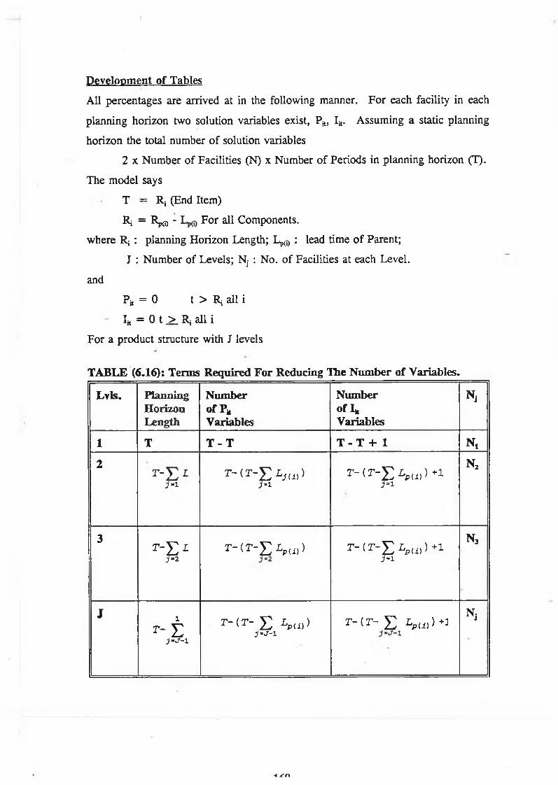
Development of Tables

All percentages are arrived at in the following manner. For each facility in each

planning horizon two solution variables exist, P*, Iit. Assuming a static planning

horizon the total number of solution variables

2 x Number of Facilities (N) x Number of Periods in planning horizon (T).

The model says

T = R, (End Item)

Ri = R ^ - For all Components,

where R< : planning Horizon Length; Lp(0 : lead time of Parent;

J : Number of Levels; Nj : No. of Facilities at each Level.

and

PH = 0 t > Ri all i

IH = 0 t _> Rj all i

For a product structure with J levels

TABLE (6.16): Terms Required For Reducing The Number of Variables.

Lvls. PlanningHorizonLength

NumberofPMVariables

Number of 1Variables

N j

1 T T- T T-T + 1 N,

2T - ^ L

J - lr - < r - E L J u )>

J - 1r - l r - E W 1

7=1

n 2

3

r - E 1J"2

T - ( T - E W r-tr-E-'W * 1J - l

n 3

JT - tj ‘ J - 1

T - { T - E l p u ) >j - j - ir-(r-E W 3

N j

1 Z-fk

Table(6.16) Develops the Various terms which are required to generate the number

of terms which must be set to zero when using the Dynamic Planning Horizon. For

each level within the planning horizon account must be taken of Production and

Inventory Variables at each facility.

£ N j [ ( T - + ( t - ( t - £ Lp U , ) +1) ) 1 ( 6 . 3 1 )j - 1 j ’ J j - J

E ' E^ii) + È^<i»+11 (6-3J)7-1 j ' j j ' j

E 12 E lp w + 1 1 <6- 33)7 -1 7-1

The term ELp© is the lead time so far accumulated within the product structure-the

sum of the lead times for the parent items at this level. At level Three for example this

term would be accumulate lead times over levels’ one and two. For the purposes of

these tests the lead time at each facility was assumed to be one and two

respectively.The sum of accumulated lead times can therefore be equated to the

number of levels.

E - J - 1 ( 6 , 3 4 )j - j - i

The equation then becomes:

j

£ [ 2 ( iJ-1)] (6*35)7-1

Eqn.(6.35) describes the number of variables to be set to zero within each product

structure. The percentage decrease in variables due to the use of the dynamic horizon

can now be easily calculated.

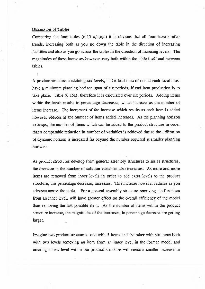
Discussion of Tables

Comparing the four tables (6.15 a,b,c,d) it is obvious that all four have similar

trends, increasing both as you go down the table in the direction of increasing

facilities and also as you go across the tables in the direction of incresing levels. The

magnitudes of these increases however vary both within the table itself and between

tables.

iiA product structure containing six levels, and a lead time of one at each level must

have a minimum planning horizon span of six periods, if end item production is to

take place. Table (6.15a), therefore it is calculated over six periods. Adding itéms

within the levels results in percentage decreases, which increase as the number of

items increase. The increment of the increase which results as each item is added

however reduces as the number of items added increases. As the planning horizon

extemps, the number of items which can be added to the product structure in order

that a comparable reduction in number of variables is achieved due to the utilization

of dynamic horizon is increased far beyond the number required at smaller planning

horizons.

As product structures develop from general assembly structures to series structures,

the decrease in the number of solution variables also increases. As more and more

items are removed from inner levels in order to add extra levels to the product

structure, this percentage decrease, increases. This increase however reduces as you

advance across the table. For a general assembly structure removing the first item

from an inner level, will have greater effect on the overall efficiency of the model

than removing the last possible item. As the number of items within the product

structure increase, the magnitudes of the increases, in percentage decrease are getting

larger.

Imagine two product structures, one with 5 items and the other with six items both

with two levels removing an item from an inner level in the former model and

creating a new level within the product structure will cause a smaller increase in

TABLE (6.15b): Percentage Decrease in No. of Solution Variables WithPlanning Horizon (Dynamic)

Level

Item

2 3 4 5 6

2 9%

3 12% 17%

4 14% 20% 23%

5 15% 22% 27% 30%

6 16% 24% 30% 34% 36%

(best case always taken - majority items on last level)

(Planning Horizon = 8)

TABLE (6.15a): Percentage Decrease in No. of Solution Variables WithHanning Horizon (Dynamic)

Level

Item

2 3 4 5 6

2 13%

3 17% 22%

4 19% 27% 31%

5 20% 31% 36% 40%

6 21% 32% 40% 46% 49%

(best case always taken - majority items on last level)

(Planning Horizon = 6)

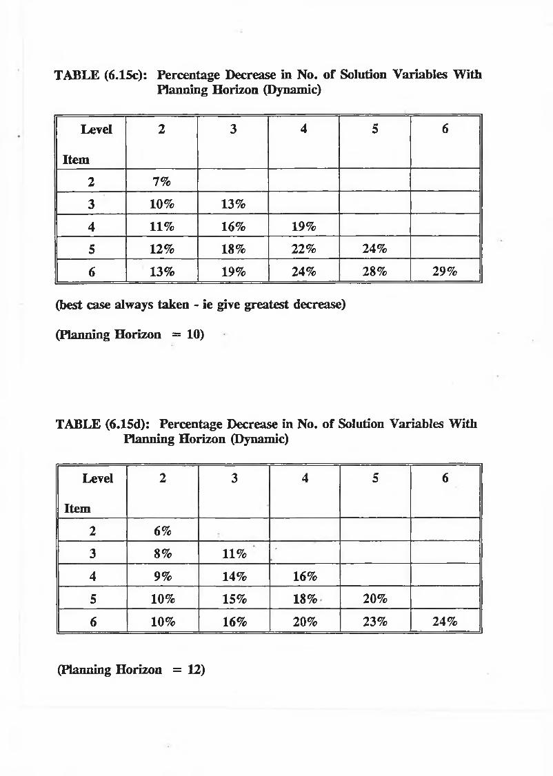
TABLE (6.15c): Percentage Decrease in No. of Solution Variables WithPlanning Horizon (Dynamic)

Level

Item

2 3 4 5 6

2 7%

3 10% 13%

4 11% 16% 19%

5 12% 18% 22% 24%

6 13% 19% 24% 28% 29%

(best case always taken - ie give greatest decrease)

(Planning Horizon = 10)

TABLE (6.15d): Percentage Decrease in No. of Solution Variables With Planning Horizon (Dynamic)

Level

Item

2 3 4 5 6

2 6%

3 8% 11% •

4 9% 14% 16%

5 10% 15% 18% 20%

6 10% 16% 20% 23% 24%

(Planning Horizon = 12)

percentage decrease than if the same were done in the six item model. However, as

both models come closer to achieving serialisation ie. one item one level this

increase, in the percentage decrease, although higher in the product structure with the

greater number of items, converges to approximately the same number.

As the planning horizon increases percentage decreases in the number of variables

decrease (due to an increase in the number of variables, before the dynamic horizon

is introduced). As the planning horizon lengthens however, the number of items

which must be added to the product structure in order than greater utilization of the

dynamic horizon is made is increased. The range of the increases incurred, by

increasing levels within the product structures also decrease as the planning horizon

advances.

Test O f Table Predictions

In order to test the predictions of Tables (6.15 a,b,c,d) the solution times of two

product structures were investigated. These product structures are shown in Fig.

(6.16). Tests were carried out in order to find the average solution solution times for

the two product structures, using planning horizon lengths, which varied from 2 to

12. The product structures were investigated firstly using no dynamic horizon,

Tables (6.18 a,b) and secondly with a dynamic horizon Tables (6.19 a,b). For each

product structure, increasing the length of the horizon resulted in an increase in

solution time. (See Appendix (7) for these results).

Comparing the practically obtained results for both product structures, in terms of

percentage decrease in solution due to a decrease in the number of solution variables,

with Tables, (6.15 a,b,c,d) the results obtained are very similar. Table (6.17)

compares the results.

Both models were investigated under conditions of varying demand, different cost

structures per period and differing quantities per parent items.

Oem.

(a)

Dem.¡1

2

! B

(b)

Product Structure. Fig.(6.16).

Table (6.17) shows that practical results are within +. 5% of theoretically obtained

percentage reductions due to the dynamic planning horizon.

TABLE (6.17): Comparison of Practical, Theoretical Effect of Dynamic Horizon.

Planning Horizon Length.

6 8 10 12

Product Structure Practical 13% 9% 7% 6%Fig. 1 Theoretical 13% 10% 6% 9%

Product Structure Practical 46% 34% 23% 28%Fig. 2 Theoretical 40% 34% 27% 23%

Conclusions

Product structures, with, small numbers of both items and levels, can obtain greater

benefits from the dynamic horizon, using a shorter horizon span. As the product

structure becomes more serialized (assuming const number of items) (ie. spread over

a greater number of levels) the dynamic horizon achieves greater benefits.

As the planning horizon lengthens, the size of the product structure required to

achieve comparable reductions in the number of variables increases. An increas in

the number of levels in the product structure causes these benefits to be achieved to

much greater magnitude.

Irrespective of planning horizon length, complex product structures, with many items

and levels, may use the dynamic planning horizon to great effect, the greater the

number of levels within the structure the greater the effect.

6.6.3 Comparison of the Various Lot Sizing Methods IntroductionThe various lot sizing methods currently in use today, are discussed in section 6.2,

6.6.3 Comparison of the Various Lot Sizing Methods Introduction

The various lot sizing methods currently in use today, are discussed in section 6.2,

and their respective advantages/disadvantages in Table (6.24). This section seeks to

show the disparity between the requirements planned using these techniques, and

those obtained using a linear programming formulation. Many manufacturers favour

a Lot-For-Lot Method of lot sizing but this also has inherent problems. Four

methods are chosen from among those discussed each representing a particular type

of lot sizing procedure.

Wagner Whitin is chosen to represent the dynamic approach to lot sizing, economic

order quantity the static approach, and period order quantity a slight mixture, where

the timing of orders is the same, but the amount ordered varies. Finally the Lot-For-

Lot method is also included. (As with all other methods, the planned quantity is

rounded to the nearest whole number). Both the economic order quantity and period

order quantity, can not accommodate changing costs per period, and so an average

cost per period is used for comparative purposes.

A three facility model is used to compare the methods, and the respective cost

structures are shown in Table (6.21a). Each model is tested over five different

demand patterns. It must be mentioned however, that the quantities required per

parent items are both equal to one, which means that the results obtained with

Wagner Whitin, Economic order quantity and period order quantity methods, applied

independently at each level, are better than would usually be expected, if this number

were greater than one in comparison to the linear programming and Lot-For-Lot

solution. The demand patterns are listed in Table (6.21b). They are lumpy, uniform,

convex, increasing and decreasing.

1 n n

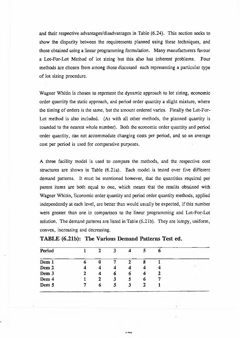
and their respective advantages/disadvantages in Table (6.24). This section seeks to

show the disparity between the requirements planned using these techniques, and

those obtained using a linear programming formulation. Many manufacturers favour

a Lot-For-Lot Method of lot sizing but this also has inherent problems. Four

methods are chosen from among those discussed each representing a particular type

of lot sizing procedure.

Wagner Whitin is chosen to represent the dynamic approach to lot sizing, economic

order quantity the static approach, and period order quantity a slight mixture, where

the timing of orders is the same, but the amount ordered varies. Finally the Lot-For-

Lot method is also included. (As with all other methods, the planned quantity is

rounded to the nearest whole number). Both the economic order quantity and period

order quantity, can not accommodate changing costs per period, and so an average

cost per period is used for comparative purposes.

A three facility model is used to compare the methods, and the respective cost

structures are shown in Table (6.21a). Each model is tested over five different

demand patterns. It must be mentioned however, that the quantities required per

parent items are both equal to one, which means that the results obtained with

Wagner Whitin, Economic order quantity and period order quantity methods, applied

independently at each level, are better than would usually be expected, if this number

were greater than one in comparison to the linear programming and Lot-For-Lot

solution. The demand patterns are listed in Table (6.21b). They are lumpy, uniform,

convex, increasing and decreasing.

TABLE (6.21b): The Various Demand Patterns Test ed.

Period 1 2 3 4 5 6

Dem 1 6 0 7 2 8 1Dem 2 4 4 4 4 4 4Dem 3 2 4 6 6 4 2Dem 4 1 2 3 5 6 7Dem 5 7 6 5 3 2 1

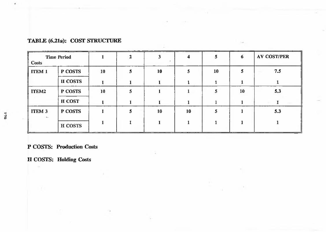
TABLE (6.21a): COST STRUCTURE

Time Period 1 2 3 4 5 6 AV COST/PERCosts '

ITEM 1 P COSTS 10 5 10 5 10 5 7.5

H COSTS 1 1 1 1 1 1 1

1TEM2 P COSTS 10 5 1 1 5 10 5.3

H COST 1 1 1 1 1 1 1

ITEM 3a .

P COSTS 1 5 10 10 5 1 5.3

II COSTS1 1 1 1 1 1 1

P COSTS: Production Costs

H COSTS: Holding Costs

Inventory holding costs are calculated on the basis of average inventory, in a period,

with inventory at the beginning and at the end of a period being taken for the average

calculations. Production costs for the Lot-For-Lot, Wagner Whitin and linear

programming solutions are based on the cost in which the requirement arises.

Economic order quantity and period order quantity production costs are based on the

average cost per period.

Once the total costs for each of the methods performance over the various demand

patterns was ascertained, a cost index was used to allow easy comparison of their

relative performance. For each demand pattern, the performances of the various

techniques were compared to the performance of the linear programming solution.

The following cost index was used.

COST INDEX = Techniques Total Cost________ X 100Linear Programs Total Cost

Table (6.22) lists the results obtained and the Lot-For-Lot method performs

consistently better than either of the other three methods, over all the demand pattern.

The period order quantity method also performs better than either of the other two

methods when dealing with all but the convex demand pattern. Wagner-Whitin

performs better than the economic order quantity method, on all but one occasion.

It may therefore be said that of all the methods the economic order quantity method,

produces results which are the farthest removed from the linear programming method.

Table (6.23) ranks each of the methods in order of decreasing efficiency, based on

a scoring method, which gives one to four marks for coming first to fourth

respectively.

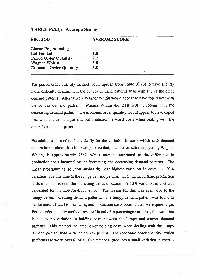
I

TABLE (6.23): Average Scores

METHOD AVERAGE SCORE

Linear ProgrammingLot-For-Lot Period Order Quantity Wagner Whitin Economic Order Quantity

1.02.23.03.8

The period order quantity method would appear from Table (6.23) to have slightly

more difficulty dealing with the convex demand patterns than with any of the other

demand patterns. Alternatively Wagner Whitin would appear to have coped best with

the convex demand pattern. Wagner Whitin did least will in coping with the

decreasing demand pattern. The economic order quantity would appear to have coped

best with this demand pattern, but produced the worst costs when dealing with the

other four demand patterns.

Examining each method individually for the variation in costs which each demand

pattern brings about, it is interesting to see that, the cost variation enjoyed by Wagner

Whitin, is approximately 28%, which may be attributed to the difference in

production costs incurred by the increasing and decreasing demand patterns. The

linear programming solution attains the next highest variation in costs, — 20%

variation, due this time to the lumpy demand pattern, which incurred large production

costs in comparison to the increasing demand pattern. A 10% variation in cost was

calculated for the Lot-For-Lot method. The reason for this was again due to the

lumpy versus increasing demand patterns. The lumpy demand pattern was found to

be the most difficult to deal with, and production costs accumulated were quite large.

Period order quantity method, resulted in only 5.6 percentage variation, this variation

is due to the variation in holding costs between the lumpy and convex demand

patterns. This method incurred lower holding costs when dealing with the lumpy

demand pattern, than with the convex pattern. The economic order quantity, which

performs the worst overall of all five methods, produces a small variation in costs, -

6.7%. The reason for this variation is similar to that of the Wagner Whitin method,

increasing and decreasing demand patterns, but in this case it is the holding costs

which cause the variation, being slightly higher using the increasing demand pattern,

than the decreasing pattern. The production costs incurred by the linear programming

solution are lower than those incurred by all other Lot-Sizing methods, for each and

every demand pattern.

The holding costs however incurred by the Lot-For-Lot method of ordering will

obviously be lower. This method is the only method which results in consistently

lower holding costs across the spectrum of demand patterns. Wagner Whitin has

lower holding costs, with the convex and increasing demand patterns and period order

quantity, using lumpy and increasing demand patterns.

The holding cost reduction however, which would be achieved by using any of these

methods, is more than compensated for by the opportunity cost, in production terms

of retaining the linear programming method.

Comparison of Lot Sizing MethodsCost Index

250

200

150

100 -

Demand 1

Wag. wh i t ,

Demand 2 Demand 3 Demand 4Lot Sizing Methods

\ord .Q. I lllll L.- f . -L . H

Demand 5

E.ord.Q iM iiiil Lin,Prog.

Fig.(6 .16)

I

CHAPTER 7

KANBAN

7.1 TYPES OF KANBAN CARDKanban is the name which has been adopted to describe the method of controlling

material on the factory floor. It is the Japanese word for card, and came about due

to the extensive use of cards (and or signals) within Just-In-Time Systems in Japan.

Two main types of cards are in evidence:

1. Production Kanban

2. Withdrawal (Move) Kanban

A production type Kanban is used to initiate production within a given work centre.

The card contains certain limited information about the piece to be processed such as

item code, description, storage area and type of processing required. The card

remains within the bounds set by the work centre, and associated input/output buffers

and kanban posts.

A withdrawal or move Kanban, is used to withdraw material from a previous process.

This type of card must necessarily move between adjacent work centres. Supervising

material flow from the output buffer of the feeder work centre to the input buffer of

the processing station. A withdrawal card, contains information regarding item codes

and description, preceding and actual processing work centres and withdrawal

quantities.

The terms withdrawal and production Kanban, have two meanings.' Primarily they

are used to describe cards which control both intra and inter production processes

which occur in a normally operating repetitive manufacturing environment. Secondly,

they are used generally to describe a variety of cards which may be required to

ensure a successful completion of the whole manufacturing process, (Monden [45]).

A supplier Kanban, (withdrawal type) is used as the name suggests to obtain raw

materials from suppliers. The Kanban contains lists of instructions regarding the

delivery of these materials. A subcontract kanban is similar to the supplier kanban

but refers to subcontract agreements.

If production on an assembly line is being fed by parts manufactured in a machine

shop, - forging, die casting etc. The idea of production, withdrawal Kanban must be

extended to the machine shop. Here where batch production predominates, the two

types of Kanban are collectively termed signal Kanban. The production ordering

Kanban, which operates like a two bin system is called a triangular Kanban, and the

withdrawal kanban, which operates in a similar fashion is called a material requisition

or rectangular Kanban.

Within any manufacturing environment deviations from the plan will occur. Several

types of kanban are available to deal with these problems. Express Kanbans, which

take the form of both production and withdrawal Kanban, may be introduced if a

preceding station runs short of parts. Emergency Kanbans, are introduced if a

particular work centre has a greater defect percentage than expected. Again

emergency Kanbans take the form of both production and withdrawal kanban and are

removed from the system as soon as the correct compensation has been made. A

through Kanban is a production ordering Kanban which also acts as a withdrawal

Kanban. Its main application would be in process type plant areas, where production

at one process area is immediately followed by processing at the next process, via and

automatic link/chute between processes. Alternately a common Kanban is a

withdrawal Kanban which performs the dual functions of both withdrawing and

producing. The two processes involved must be distinct but very close together.

7.2 RULES ASSOCIATED WITH KANBAN OPERATION

In much of APICS literature describing the emergence of MRP II in America, a great

deal is made of the need to establish formal procedures, from within which MRP can

operate efficiently. In some respects, kanban, which has no central control

mechanism, unlike that of MRP, requires that even greater emphasis is placed on the

establishment of these procedures.

I

The first rule of Kanban production and its’ associated corollories echoes this

sentiment.

Rule 1 "The subsequent process should only withdraw the

necessary products from the preceding process and in

the necessary quantities at the correct point in time".

Corollories 1. A kanban should always be attached to a physical product.

2. Any withdrawal greater than the number of kanban should be

prohibited.

3. Any withdrawal without a kanban should be prohibited.

Together, the above rule, and its corollories place control of the withdrawal process

form one work centre to the next, in the hands of workers on the factory floor.

The second rule for kanban production describes the quantities in which production

takes place. Again, unlike MRP, where requirements for each and every work centre

are determined by a central control, the correct production quantities are determined

by the worker based upon quantities withdrawn to feed subsequent processes.

Rule 2 "The preceding process should produce its products in

the quantities withdrawn by the subsequent process".

Corollories 1. Production greater than the number o f kanban sheets must be

prohibited.

2. When various kinds of parts are to be produced in the preceding

process their production should follow the original sequence in which

each kind of kanban has been delivered.

The second corollory, underlines the need for set-up time reduction, if kanban

implementation is to be successful. If set-up times at the preceding process are

prolonged then there will be a long delay between request and delivery of parts,

disrupting the flow of parts. In effect a bottleneck is created.

One of the major differences between Kanban and MRP, is that MRP in the simplest

sense operates on the pretence that nothing can go wrong. When it does, all the

information regarding the incident is feed back into the computer (closing the loop),

and new decisions are made at this central control, to compensate for the incident.

This information flow can be very time consuming. Conversely, Kanban, in

realization of this time delay, deals with incidences as they occur on the factory floor.

This is accomplished in some respects by making the operator, responsible not only

for the correct production of parts, but also for thè quality of production. Rule three

states.

Rule 3 "Defective products should not be conveyed to the

subsequent process”.

If defective parts are conveyed to the subsequent process, the process runs short of

parts, and line stoppage results. The cause of the quality problem, is also of prime

concern to the operator. Badly kept tools, routines, labour hours, cause quality

problems, and must be accounted for by the operator, in his goal to perform Total

Preventative Maintenance.

In a factory which is driven by MRP, or in fact, by any push system, work-in-

progress (WIP) can make'up a high percentage of overall factory inventory. Unless

interpreted correctly, the level of WIP in a system, can falsely represent now well a

system is operating. High levels of work-in-progress serves to hide operating

problems and in deference to this, JIT practitioners refer to lowering the river of

inventory to expose the rocks (operating problems). Using a Kanban system, (as will

be explained Section (7.4.1 )), it is the number of kanban cards in the system, which

ultimately decides the level of inventory in the system. Using a dual card system, at

a particular point in time, assume no production at work station y, and empty kanban

posts, the maximum WIP level at the input and output buffers is determined by the

number of withdrawal and production kanbans respectively. Decreasing the number

of cards therefore reduces the amount of WIP in the system. Rule four states.

Rule 4 "The number of kanbans should be minimised".

1 O f

Reducing the set-up time, means that the lot size can be reduced, which in turn, can

cause a lead time reduction. Noticeable reductions in cycle time, mean that the

number of parts in simultaneous production can be decreased. This is achieved by

removal of kanban cards from the system. The determination of an optimum number

of cards to control the systems performance must then be followed by policies to vary

cycle times in response to fluctuations in demand. For example, if demand is

increased the system which is operated by a multi-function work-force can move

workers from a low demand to a high demand area thereby increasing capacity. Any

problems which surface during operation are immediately identifiable, due to low

WIP values, and solutions can be found quickly.

An MRP system, generates requirements for each and every process within the

system, at fixed intervals based on demand. Dependant on the type of system in use,

these requirements are then used to generate production schedules. Large fluctuations

in demand or deviations from forecast, require rescheduling for each and every

process within the system, which can cause unnecessary time delays between due date

and finish date. Unlike MRP, kanban requires only one valid schedule. The final

assembly schedule which dictates the daily build quantities. If at the end of the day,

a change in the plan is required this can easily be accomplished by changing only this

one schedule. The final rule for kanban production states.

Rule 5 "Kanban should be used to adapt to small fluctuations

in demand".

If the final assembly schedule is balanced (uniform workloads) over a particular time

span, and a sudden increase in demand is forecast (known) in the near future. Rather

than waiting until the period becomes current, and issuing production schedules to the

floor, kanban advocates the fine tuning or rebalancing of the final assembly schedule

until the schedule is again on target. The downstream processes, are not issued any

formal notice of the change, all that happens is that cycle times may be minutely

increased, (Schonberger [32], Monden [45]).

7 3 SMOOTHING PRODUCTION

Just-In-Time production requires that variations in demand are hidden beneath a

developed uniform workload. This idea of adapting production requirements to

demand variations is referred to as production smoothing.

Smoothing necessarily requires deviations from the more typical batch manufacture,

where a single product may be produced in large batch sizes, to a situation where a

single line may produce many varieties of product each day in response to customer

demand. The method of adaptation occurs on two levels and is an integral part of the

development of the final assembly schedule. JIT manufacturers would initiate

production plans by the development of a yearly production plan in terms of model

and quantity, a two step monthly plan then follows, consisting of:

A. Models and quantities, two months previous.

B. Detailed Plan, one month previous.

If the yearly plan deviates markedly from the original plan, then this requires a

change in the monthly plan, - monthly adaptation. The monthly plan is used to

generate, daily production quantities in terms of models and model variations. For

example if 100 units per month of model A are required and, there are 20 working

days per month,

TABLE 7.1 Smoothing Production

Type M onthlyDemand

Av Daily O utput Cycle Time

A1 20 1 480 min/shftA2 40 2 96 min/unitA3 40 2

100 5

The correct proportions are listed in Table (1). An increased demand of 20

units/month, would cause an increase of 1 unit per day, requiring fine timing of

production using Kanban and a revised sequenced schedule.

Large increases or decreases in production requirements require more tangible

changes to the existing production system. Increasing overtime, hiring temporary

workers, moving skilled workers, making use of slack machinery are all incorporated

to help with increased deamdn. Slumps in demand, are not followed by massive

redundancies, although temporary workers would be let go. Idle workers are gamely

employed in quality circle meetings, practising set-ups, maintenance etc.

7.4 KANBAN MODELS7.4.1 Two Card Model

In order to operate a two card kanban system correctly, each production process

requires two buffers, input and output buffer, two kanban posts, one for production

cards and the other for conveyance cards, and inventory in each buffer. Fig. (7.1),

shows each of these elements, at two processes within an assembly line, where

material, is processed at stage N + l , and then moved to stage N. (Villeda [24]).

Daily requirements are introduced to the line via a daily requirements schedule at

final assembly. These requirements are then transmitted to every stage on the line

through the use of production and withdrawal kanban.

Before production is initiated the line is in a state of balance, with empty kanban

posts and input and output buffers filled to capacity, accompanied by the appropriate

kanban card, (material in the input buffer is accompanied by withdrawal cards) at

each and every station on the line (Table (7.1) line a). The introduction of the

schedule initiates production in the following manner.

Final iAssembly.

IJULProduction

Kanban Post. tII

a

Stage N0 2

iOutbound StocE

iProductionA ÆActivity.

I I* ! !

........................----------------------------------------------------- 1

Inbound Stock. CL>

!

Move Kanban Posi-

* t

Flow of Kanban Cards(Two Card System). Fig. (7.1)

rvA

Two Card Kanban. Fig (7.4)

191

TABLE (7.2): Postion Of Cards/Processed Units At Certain Points In Time

Production Card Post:

Stage N + l

InputBuffer:

OutputBuffer:

Withdrawal Card Post:

StaçeN +2 ( F i n a l Assembly)

Withdrawal Card Post:

(a)Balanced

------- i \ w N+1 1P2> P n+i ------- w N+2

(b)Unbalanced

(c)Unbalanced

I*N+1 1,W N+1

1 \ P n+i w N+1

(d) ------- 1U3, WN + 1 1P1J I*N+1 •»_—

WN+1 Withdrawal Card Stage N + l ; PN+1 Production Card Stage N + l

l uk Unprocessed Material Unit ( k = l k, different units);

l pk Processed Unit

A withdrawal card (WN+2) is taken to the penultimate station ( N + l ) on the line,

(which is in a state of balance, and the appropriate amount of material carried to final

assembly. The production card which accompanied the material in the buffer is

replaced in the production kanban post. (Table 7.2 line b). The station is now

unbalanced, and in order to return to a state of equilibrium must unbalance the

preceding station.

Balancing or returning to equilibrium is achieved in two steps. Firstly the production

card is removed from its post, and taken to the input buffer, and the correct amount

of material removed for processing. The accompanying withdrawal card is replaced

on its post. The input buffer is now empty, and the output buffer is again full (Table

7.2 line c). The withdrawal card is then carried to the input buffer of the preceding

process and the correct amount of material removed. This material is then placed in

the input buffer of the current station accompanied by the production card. The

station is again balanced. (Table 7.2 line d). The preceding station is now

unbalanced. Because each station is successively unbalanced, and strives to return

to equilibrium, a type of action/reaction ripple is sent down the line from final

assembly.

The level of inventory at both input and output buffers, when the system is in a state

of equilibrium (i.e. the maximum WIP level) is set by the number of cards for that

process. The exact number of cards introduced is a management decision although

formulae have been-developed. This number however should be reduced as low as

possible, without causing any disruption to the systems performance. Fig. (7.4), is

a flow chart representing the various decisions which must be made in order to bring

the system back to equilibrium.

7.4.2 Single Card Kanban

Single card kanban varies slightly from the dual card system, in that production is

carried out at each station, based upon a production schedule. Withdrawal of parts

however occurs via kanban cards. In order to operate the system correctly, each

process requires, an output buffer filled to capacity, and a withdrawal kanban post.

(See Fig. (7.2)). The line is in a balanced state, when both the output buffers and

kanban posts are filled with both material and cards respectively.

Production is initiated as follows: A final assembly withdrawal card is brought to the

preceding stage, stage N and the appropriate material removed, and immediately

processed at final assembly. Stage N is now unbalanced, because the stock level in

the output buffer is less than that at a balanced state. In order to regain balance, a

withdrawal card is brought to the preceding stage, and the correct part processed at

stage N, and placed in the output buffer. The withdrawal card is replaced on the post,

as soon as production is initiated. Stage N, has now regained equilibrium, bu the

preceding stage is now unbalanced. Each process is successively unbalanced in a

similar fashion to that of two card kanban and so again an action/reaction ripple is

sent down the line. Fig. (7.3) shows a flow chart of decisions required for each

process to return to equilibrium.

1 m

Final ♦ Assembly.

Stage Nu

A

I I I

Outbound Stock

production

I------- \

u .Move Kanban P6s

»

Flow of Move Kanban Cards(Single Card Kanban). Fig.(7.2)

1Q 4

CheckProductionSchedule.

Wait

Wait

Process Part.

Stop

Single Card Kanban. Fig. (7.3)

CHAPTER 8

A SIMULATION STUDY OF KANBAN SYSTEMS

8.1 SIMAN AND SIMULATION

8 .1 .1 I n t r o d u c t io n

Simulation is used in a wide variety o f fields to mimic the dynamic behaviour of real

systems, as time proceeds. A system, may be defined (Schriber [49]), "As a

collection of interrelated elements which work together co-operatively for the purpose

of achieving a stated objective".

Two basic types of simulation exist, namely, discrete event and continuous

simulation. The former describes a system in which all changes in state occur at

specific points in time. (eg. parts arriving at an input storage buffer). The latter type

- continuous - refers to the case where all changes in state occur continuously over

time (eg. chemical processing). Hybrid systems, made up of both types also exist.

Within the confines o f a manufacturing system, simulation may be undertaken for a

wide variety of reasons. It may be used to monitor or evaluate proposed changes in

resource capacity requirements, where the resource in question may be a machine,

or personnel, transporter mechanisms, or even work-in-progress buffers. When

modifications, or complete replanning of specific system areas, such as a change in

machine layout, or change in product mix, or even a change in product scheduling

method is suggested, simulation can be used to great effect, in evaluating the various

proposed methods.i *

8 .1 .2 I n t r o d u c t io n to S I M A N

In order to perform a simulation, a simulation model must be built. Various high

level computer languages exist for this purpose - GPSS, SLAM II, GALS etc.

SIMAN is a general purpose simulation analysis package, which allows the modelling

of combined discrete/continuous systems.

The modelling framework of SIMAN, allows the various models to be logically split

into two distinct and very separate sections. The first o f these sections is termed the

system model - and defines the "Static and dynamic characteristics o f the system".

The second section, termed the experimental frame, "defines the experimental

conditions under which the model is run" (Pegden et al [50]). Various parameter

values, resource capacities, and processing sequences are defined within this section.

This separation of the model into two distinct sections means that the same model can

be run under a variety of performance conditions, using different experimental

frames. Before the simulation run, both sections o f the model must be compiled and

linked together.

The standard form of the output generated by the SIMAN program consists o f an

average o f model state transitions as they occur over time. The actual transitions o f

interest are stated as performance measures within the experimental frame. The

period o f time which the statistics reflect is also listed in the experimental frame.

The generated output file may be investigated further through the use of the SIMAN

output processor.

A SIMAN system model file is specified in terms o f blocks. To facilitate

programming each block has an associated pictorial symbol and top down flow charts

can be drawn and ten basic building blocks to define a system model. The

experimental frame, is defined in terms o f elements. Each element providing more

information about the system, The parameters element for example, gives the various

parameter for any experimental distributions referenced in the model. The resources

element names and defines the capacities o f the various resources. The transporters

element does the same for transporters. The sequences element defines the various

sequences between machines which an entity might take. Once the model file has

been developed, the experimental frame, is relatively easy to write. Parts, and people

etc, within a SIMAN file are represented by entities, which flow through the system.

Entities may be personalised by assigning various attributes (A(*)) to them.

8.2 SIMULATION OBJECTIVES

Many authors have investigated the effects o f the process time imbalance (see Sarkar

et al [22]) on push production systems. Recently this work has been extended to

cover pull systems also. Villeda et al [24], has done work in this area.

One type of process time configuration - referred to as the "Bowl - Phenomenon" is

thought to be caused by:

A. Imbalance in work station mean

B. Imbalance in work station variability.

This study will examine the effects of both, on systems performance, with a bowl

type configuration and with the alternate configurations described in Section (8.6).

Any effects in system performance due to process time variability can be overcome

by increasing the level o f work in progress (WIP) within the system. WIP however

is also undesirable, and a secondary objective therefore is to find that value o f

maximum buffer stock which allows control o f system performance through process

time variation. This also allows an investigation in the change in system performance

parameters with an increase in the number of cards within the system.

8.3 PERFORMANCE MEASUREMENTS

8.3.1 Introduction

The problem which confronts any model builder is to accurately ascertain how the

system is performing. One of the more obvious measures is the time a part spends

in the system, from creation to completion. This type of measurement, which is

purely observational is easily accomplished by counting the entities as they pass some

point in the model, and noting the time which has elapsed. Cycle times for parts

within the system may be found in this manner.

In order to find data on such topics as resource utilization or the average number o f

parts in various buffers, time dependant performance measurements muct be called

upon. Time dependant data consists o f a sequence o f values, the value o f which

persist over some specified amount o f time. This value must be weighted by the

amount o f time that for which value exists. Time dependant data must be recorded

whenever the value o f the time dependant variable changes. If the number o f entities

(parts) residing in a particular queue are of particular interest, then each time the

length of the queue varies both this value, and the time for which the queue remains

at this length must be recorded. The average value of machine utilizations, may be

computed in this fashion.

The SIMAN language, allows easy collection of both observational and time

dependant data, through the use o f a TALLIES and DSTATS elements respectively.

8 .3 .2 E v a lu a t in g T h e K a n b a n M o d e ls P e r fo r m a n c e

The performance measures used to evaluate the models performance were of two

types: - primarly and secondary measures. Primary performance measures, were

those from which it is immediately possible to gauge a systems performance, namely

the production rate (per shift) and the level o f WIP in the system. Secondary

performance measures, which provide more information about the internal working

of the system were also evaluated. These measures included mean resource

utilization figures, and also mean waiting time for final assembly, (ie. the length of

time a part waits for all three parts to be made available).

8.4 THE PROBLEM SPECIFICATION

A production line is perfectly balanced, when the processing times at different stages

are the same. In this situation the operators at each station have an optimum

inventory pile to work from and no blocking or starving occurs at any work centre.

Blocking is said to occur (Silver et al [51]) when a work station, having completed

a part, finds the next buffer, filled to capacity and therefore must retain the part until

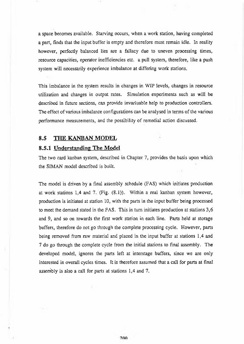
a space becomes available. Starving occurs, when a work station, having completed

a part, finds that the input buffer is empty and therefore must remain idle. In reality

however, perfectly balanced lies are a fallacy due to uneven processing times,

resource capacities, operator inefficiencies etc. a pull system, therefore, like a push

system will necessarily experience imbalance at differing work stations.

This imbalance in the system results in changes in WIP levels, changes in resource

utili2ation and changes in output rates. Simulation experiments such as will be

described in future sections, can provide invarluable help to production controllers.

The effect o f various imbalance configurations can be analysed in terms of the various

performance measurements, and the possibility o f remedial action discussed.

8.5 THE KANBAN MODEL

8.5.1 Understanding The Model

The two card kanban system, described in Chapter 7, provides the basis upon which

the SIMAN model described is built.

The model is driven by a final assembly schedule (FAS) which initiates production

at work stations 1,4 and 7. (Fig. (8.1)). Within a real kanban system however,

production is initiated at station 10, with the parts in the input buffer being processed

to meet the demand stated in the FAS. This in turn initiates production at stations 3,6

and 9, and so on towards the first work station in each line. Parts held at storage

buffers, therefore do not go through the complete processing cycle. However, parts

being removed from raw material and placed in the input buffer at stations 1,4 and

7 do go through the complete cycle from the initial stations to final assembly. The

developed model, ignores the parts left at interstage buffers, since we are only

interested in overall cycles times. It is therefore assumed that a call for parts at final

assembly is also a call for parts at stations 1,4 and 7.

Workstation Layout. Fig.(8.1)

The described model (Chapter 7), refers to withdrawal and production kanban cards.

These cards set the level of buffer stock at the input and output buffers. When all the

cards are in use, the number o f parts in the input buffer cannot exceed the number

o f withdrawal cards and similarly the number in the output buffer cannot exceed the

number of production kanban. With only one part being routed from one station to

the next, it is possible to allow the set maximum level o f work in progress at input

and output buffers at each station represent the number o f withdrawal and production

kanban respectively.

8 . 5 . 2 T im e D e la y s W ith in K a n b a n M o d e l

For each operation within the system, there can be at most six types o f delays. The

first o f these delays is a queueing time delay, and is the elapsed time from when a

part enters an input buffer, to that time when it seizes the top position in the buffer.

This time is not fixed within the model, but rather is dependant upon system

performance and is determined by the system. (Fig. (8.2), D l) .

The second time delay occurs if a part at the top of a buffer (assuming first in first

out) must await the arrival of a production kanban, in order that production .can be

initiated. If the correct card is not available this means that the actual machine

involved in processing is busy. (Fig. (8.2) D2).

The next time delay which occurs is the actual processing time at the machine in

question. This time delay is built into the model, and impacts on the systems

performance (Fig. (8.2) D3).

Once a part has been processed, the part must be moved to the output buffer.

However, if the output buffer is filled to capacity the part must remain with the

machine until space is available. This time delay, is obviously again dependant upon

the systems performance (Fig. (8.2) D4) (Blocking).

Stage N D 5O u t¿U t Buf lier

Production

Kanban.

D2 — D3 — D4Awaiting

D1Input But fjer

D7 D6

Stage N+1 AwaitingWithdrawal

Kanban.

111 ; l

05

Production.Outpiut Buff 1er.

i

. — D3 D41

Key.

C ode D e lay

D1 dueue (Input Buffer)D2 Wait (Machine in use)D3 P ro ce ss TimeD4 No Space in 3uffer(0utput)D5 Queue(Output 3uffer)06 No Space in 3uf ferì Input)D7 Routing Time

Time Delays Within the Kanban Model. Fig. (8.2)

The next time delay to be incurred is that of storage time in the output buffer, ie. the

time the entity takes to become current. (Fig. (8.2) D5).

When the part arrives at the top of the store a check must be made before the part is

routed to the next station. If withdrawal cards are in use, the arrival o f a withdrawal

card signifies a positive check and the part may be moved. Otherwise the part must

reside at the top o f the store until a card becomes available. (Fig. (8.2) D6).

A routing time, ie the time it takes for a part to be routed from one station to the next

may also be incurred. This time, like operating times, is built into the model.

8 .5 . 3 A s s u m p t io n s O f M o d e l S y s te m

1. The system processes only one product type.

2. This product is produced on the multi-line, multi-stage assembly system laid

out in Fig. (8.1).

3. Each process shown in Fig. (8.2) has two associated buffers - one for both

input and output stock.

4. The amout of stock allowed to reside in these buffers, is set by the maximum

number of move and production kanbans existing at that work centre.

5. Final assembly is producing Just-In-dme, as dictated to by requirements.

6. Processing times at each work station are assumed to be normally distributed,

with a mean o f 15, unless otherwise stated. Three different coefficients of

variation (CV) are used.

7. Demand for parts at final assembly occurs exponentially, with a mean of 8

0* * 8).

8. The routing time between work station is assumed to be zero.

9. No scrap or defective parts are produced at any work station.

10. The objective is to maximise the number o f parts/entities completed per 480

min shift.

8 . 5 . 4 S im u la t io n M o d e l - S I M A N

A simulation run using SIMAN, requires at least two files.- A model file and an

experimental file. The model file describes the flow of parts (entities) through the

various processes within the model. Each piece o f code is called a block. The

experimental file is used to provide more information about the blocks in the model

file. The files used to simulate the kanban model are listed in Appendix (4).

The Model File

The first section o f the model file is used to generate a final assembly schedule. The

time between creations are exponentially distributed. As explained in section (8.5.1),

a call for parts at final assembly, equates to a call for parts at the first station in each

line, and therefore each time a part, is written to the final assembly schedule, three

dublicate entities are created, and assigned their respective attribute values. These

entities are each sent on separate routes towards final assembly.

The second part o f the file deals with entity flow through the assembly system. The

system (Fig. (8.1)) shows ten processing areas and each o f these are correspondingly

modelled as work stations 1 through 10. Each work station contains three vary

important elements - An input buffer (queue M, where M is the number o f the

present station), the actual processing resource (Work Centre M), and an output

buffer, (Queue M + 30). Within a kanban model, the movement o f parts from buffers

to work centre, within a station, and from buffer to buffer between stations must be

carefully controlled. This is achieved within the model by use of a SIGNAL and

WAIT block combination. One of the part specific attributes, an entity gains on

creation is the station number of the next station to be visited by that entity. (This

is automatically updated via the SEQUENCES element as a part enters a station).

Before a part can be moved from its present position at an output buffer to the input

buffer o f the next station, a check must be made to see if the input buffer has space

available. The capacity o f each input buffer is specified as a global variable

(X(A(1)). If there is no space available at the input buffer the part (entity) is held in

a WAIT block until a space becomes available, and a signal corresponding to the first

operand of the WAIT block is received. This signal is sent by a SIGNAL block as

soon as the work centre has been seized, indicating that a part has been removed from

the buffer. Once this signal has been received, the entity leaves the WAIT block, and

checks again to see if there is space available at the buffer. If there is, the entity is

sent to the input buffer, if not, it is sent back to the WAIT block to await another

signal.

A similar situation arises when a part is moving from a work centre to an output

buffer. A check is made to see if there is space available on the output buffer, if

there is, the part moves, otherwise the part enters a WAIT block to await a signal,

which is sent as soon as a part departs the output buffer. This time however signal

values vary from 11 - 20, instead of 1 - 10.

The final assembly authorises production which is initiated at stations 1,4 and 7, (see

section (8.5). It is therefore necessary to make three duplicates of the authorisation

entity to send to each o f these stations.

All the time assembly station are dealt with within the same macro submodel, and is

necessary therefore to include a number of BRANCH blocks with this macro. When

an entity reaches stations 3, 6 or 9, instead o f checking immediately to see if there

is space available at the input buffer of station 10, before being routed to station 10,

an entity reaching any of these stations must wait until an entity has been processed

at the other two stations. All three entities may then be simultaneously released and

permanently combined, before, being processed at station 10.

In order to calculate the lead times for the various processes involved. Two modifier

blocks must be introduced these are the MARK block and the INT block. The

MARK blocks assigns to an entity specific attribute, the present time-tnow; and the

INT block, accumulates the elapsed time between tnow and the time when the entity

enters the associated TALLY block.

When production has been completed, and the entity has contributed to collected

statistics, the entity has fulfilled its use and must be destroyed. This is again

accomplished by a block modifier, - the DISPOSE block.

The Experimental File

As stated previously, the experimental file provides more information about the

assembly system described in the model file.

The DISCRETE element places a limit on the number of entities which can co exist

within the model at any time, and also on the number o f stations, queues and entity

specific attributes.

The RESOURCES element numbers and names the various resources within the

model, but may also be used to provide more information on the available capacities

of a particular resource, as time changes.

The model uses global variables to specify the maximum capacity o f each stock point

(ie the number o f Kanban cards available). Values may be assigned to each global

variable using the INITIALIZE element.

The SEQUENCES element is one of the most important of all elements. In its most

basic form these block, specifies the various sequences, in terms o f work stations by

which an entity may traverse the assembly system. Each time an entity encounters

a ROUTE block, with sequence as an operand, the SEQUENCE element must be

referred to.

When an entity is routed to a station via the use of a SEQUENCE element, the entity

is automatically given two new attributes, IS and NS. The NS attribute, corresponds

to the sequene number currently, in use and the IS attribute, the current sequence

index corresponding to that sequence number. Both of these attributes are updated

on entering a station.

The SEQUENCE element may also be used to change the values o f user assignable

attributes. For example, the sequences element may be used to update the attributes

associated with processsing dmes and the station to be visited. User assignable

attributes are also updated when the entity enters a new station.

The PARAMETERS element is used to specify any parameters associated with

distributions specified in the program. The first number in the distribution acts as an

index into the parameters element.

The DSTAT and TALLIES elements are used to provide system specific information.

8.6 RESEARCH PROCEDURE

1. The developed model was run for‘a variety o f parameter values. In the

’Balanced’, ’Cantilever’ and ’See-Saw’ cases, processing times were varied

from 5 - 2 5 min in steps of 2 minutes. The two ’Bowl’ configurations were

varied from 14-16 min in steps o f .2minutes. (Each set of mean processing

times were run with 3 variance values).

2. Unless otherwise stated, the number of production (and move) Kanban was set

to 1.

3. The simulation program was run for one replication o f 530 min with statistics

being cleared after 50 min for the range of processing times and system

configurations. Two random number streams were used.

4. The above procedures were initially carried out for four different unbalancing

methods described below. Initially, the second stock point was assigned a

capacity of zero, to increase the systems sensitivity.

Balanced Case

This is the base case for the study. The operation times at each workstation

in each assembly line are normally distributed, with a mean o f 15 minutes,

and a variance of 1 minute, 3 minutes and 5 minutes.

In the proceeding experiments, which are conducted in each case for the

variances listed above, when operation times are varied at certain stations, the

unvaried station retains a mean of 15 minutes.

C a n t i le v e r C a s e

In this case the first station in each line is varied, form 5 to 25 minutes in

steps of 2 minutes.

S e e S a w C a s e

Here the first and last stations in each o f the three lines are varied. As the

first station increases from 5 to 25, the last station simultaneously decreases

from 25 to 5, in steps of two.

3 Stage Bowl

In this case again only the first and third stations are varied. Both stations are

varied by a similar amount in the same direction - from 14 to 16 in steps o f

0.2 minutes.

4 Stage Bowl

In this final case the second and third station in each line are varied, while the

first station remains constant with a mean of 15 minutes. The stations are

simultaneously varied over a mean of range 14-16 minutes, in steps of 0.2

minutes.

5. The unbalancing method with the greatest potential to increase the systems

performance was identified, and steps 1-3 carried out using three sets o f card

systems.

6. The effect o f variability at the final assembly station (for the config. used in

step 5) was investigated, varying the processing time from 5 - 2 5 min, using

the three variance values. Each run was carried out according to steps 2 and

3.

8.7 DISCUSSION OF RESULTS

8 .7 .1 I n v e s t ig a t io n o f t h e U n b a la n c in g M e th o d s

SYMBOL MEANING

O • = 1

À 0 = 3

• 0 = 5

Pro

du

ctio

n

Ra

te(u

nit

s).

SYMBOL MEANING

P r o c e s s Time R a t io

Production Rate Vs. Process Time Ratio(See-Saw). Fig.(8.3b).

Pro

du

ctio

n

Ra

te(u

nit

s)

0.33 0.47 0.60 0.73 0.86 1.0 1.13 1.2 6 1.40 1.53 1.67

P r o c e s s T im e R a t i o

Production Rate Vs. Process Time Ratio(3-Stage Bowl). Fig.(8.3c).

Pro

du

ctio

n

Ra

te(u

nit

s)

0.933 0.947 0.960 0.973 0.987 1.0 1.013 1.027 1.040 1.053 1.067P r o c e s s T im e R a t i o

Production Rate Vs. Process Time Ratio (4-Stage Bowl). Fig.(8.3d).

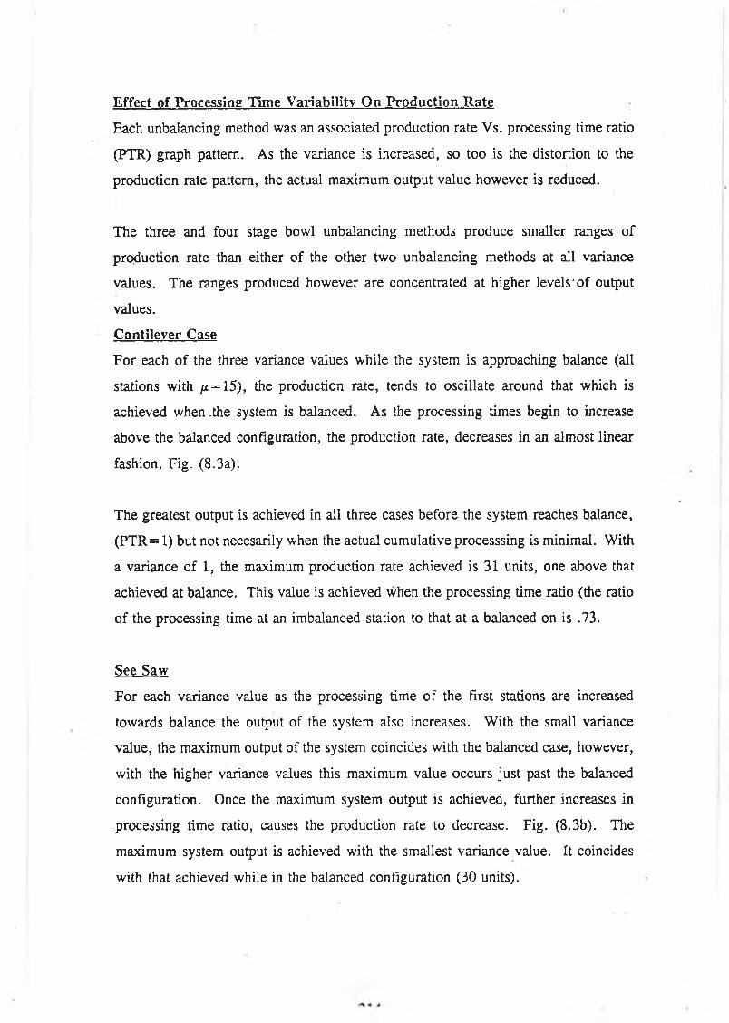
Effect of Processing Time Variability On Production Rate

Each unbalancing method was an associated production rate Vs. processing time ratio

(PTR) graph pattern. As the variance is increased, so too is the distortion to the

production rate pattern, the actual maximum output value however is reduced.

The three and four stage bowl unbalancing methods produce smaller ranges of

production rate than either o f the other two unbalancing methods at all variance

values. The ranges produced however are concentrated at higher levelsJo f output

values.

Cantilever Case

For each of the three variance values while the system is approaching balance (all

stations with /¿ = 15), the production rate, tends to oscillate around that which is

achieved when .the system is balanced. As the processing times begin to increase

above the balanced configuration, the production rate, decreases in an almost linear

fashion. Fig. (8.3a).

The greatest output is achieved in all three cases before the system reaches balance,

(PTR= 1) but not necesarily when the actual cumulative processsing is minimal. With

a variance of 1, the maximum production rate achieved is 31 units, one above that

achieved at balance. This value is achieved when the processing time ratio (the ratio

of the processing time at an imbalanced station to that at a balanced on is .73.

See Saw

For each variance value as the processing time of the first stations are increased

towards balance the output of the system also increases. With the small variance

value, the maximum output of the system coincides with the balanced case, however,

with the higher variance values this maximum value occurs just past the balanced

configuration. Once the maximum system output is achieved, further increases in

processing time ratio, causes the production rate to decrease. Fig. (8.3b). The

maximum system output is achieved with the smallest variance value. It coincides

with that achieved while in the balanced configuration (30 units).

3 Stage Bowl

In this case a graph o f production rate Vs. PTR produces an interesting step type

graph, although this is distorted slightly with the higher values o f a. In all three

cases output, decreases as balance is approached, but maximum values are attained

when the PTR values are very small (0.33 - 0.47). As the system moves away from

its balanced position production rates continue to decrease, although, with the higher

variance values, this trend fluctuates slightly. Fig. (8.3c). The small variance value

again produces the greatest production output. - 32 units, which is two units above

the balanced configuration.

4 Stage Bowl

The graphs presented for this configuration bear considerable resemblance to those

produced by that of the 3 Stage Bowl. As the system configuration tends towards

balance, (and the processing times of the 2nd 3rd stations increase), the output

reduces, although as the variance increases, slight fluctuations occur. With the small

to medium variance values, maximum output values occur when stations 2 and 3 have

small PTR values, with the higher variance value however, the maximum output is

again reached just before balance (Fig. 8.3d).

Effect of Processing Time Variability On Cycle Time

It would appear from the cycle time graphs that when utilizing either a see-saw or

cantilever configuration, the actual variance values achieved do not produce large

changes in cycle times. Using a bowl configuration however, the actual variance

values effect on cycle times are much more marked.

Cantilever

At low values o f process time ratio, the cycle times o f each o f the variance values,

are concentrated within a specific area, and show similar trends. As the system

approaches balance however the cycle times at the different values tend to separate,

with the largest variance value exhibiting the longest cycle time and the smallest

variance value the shortest cycle time. As the system moves away from the balanced

Cyc

le

Tim

e(m

in.

P r o c e s s Time R a t io

Overall Cycle Time(Cantilever).

SYMBOL MEANING0 « = 1

A » = 3• » = 5

-I-------------- 1---------------1___________ I___________I___

1.13 1.26 1-4 0 1.53 167

F ig.(8.4a).

cycl

e T

ime(

min

.

P r o c e s s Tim e R a t io

« „ 1 1 r> I rm- <-o

SYMBOL MEANINGO 0 = 1

▲ # = 3• 0 = 5

-1------------------ 1-----------------_L---------------- 1-----

1.26 U O 1.5 3 1.67

- J _________I_________ I_________ I_________ I_________ 1__0,933 0.947 0.96 0 0.973 0.987 1.0

P r o c e s s Time R a t io

Overall Cycle Time(3-Stage Bowl).

MEANINGSYMBOL

1.013 1.027 1.040 1.053 1.067

Fig.(8.4c).

_ J _ _ _ _ _ _ _ 1_ _ _ _ _ _ _ 1_ _ _ _ _ _ _ 1_ _ _ _ _ _ _ I- - - - - - - - - - - - L0.9 33 0-947 0.960 0.973 0.9S7 10

P r o c e s s T in e R a t io

Overall Cycle Time(4-Stage Bowl).

SYMBOL MEANINGO « = 1A * = 3• « = 5

I1.067

configuration, the cycle times of all three variance values tend to concentrate in a

similar region agin (Fig. 8.4a).

The general trend of this cycle time graph is upwards and increasing, although the

slope is not as great at lower values of process time ratio. This is fairly consistent

with the production rate graph, which it exhibits fairly constant output rates up to

balance, however as the cycle times increase, production rates drop. The minimum

cycle time obtained with a variance of 1 is 126 minutes, which is achieved at balance.

See Saw

With low values of process time values. The cycle times of the variance values

intermingle and are concentrated in a similar region. However as the balanced

configuration is approached, the cycle times of the three variance values separate.

Moving away from balance however the three variance values again become

entwined.

The general trend o f the graph is concave, which is fairly consistent with that o f the

production rate, which is convex, over the same x axis range. The trend o f the graph

would seem to imply that with the see saw configuration, it is the cumulative

processing time along the line which determines the cycle time, rather than the way

in which the time is distributed. (Fig. 8.4b).

The maximum cycle time is obtained with the smallest variance (126 minutes)

however the range of cycle times obtained is the largest of the three variance values

investigated.

3 Stage Bowl

Here the three variance values do not exhibit similar trends. At low values o f process

time ratio, the three variances exhibit cycle time values which are relatively far apart.

This may be accounted for by considering the greater range of production rate

achieved across the spectrum of variances at the lower end of the process time ratio

scale, in comparison to the previous system configurations. As the configuration

approaches balance, the three variances begin to converge slightly, but diverge

markedly to pass through the balanced state. Once apart, the variances remain apart,

- with the two lower values au and <r3 exhibiting similar trends-, until the end, when

all three variances converge to a similar range. (Fig. 8.4c).

The graph demonstrates that when the bowl is convex, ie. lower processing times

assigned to work stations 1 and 3, the effect of an increase in variance is not as

marked as that seen when the bowl is concave. The general trend o f the graph is

linear in keeping with the small range of production rate.

The mimimum cycle time (126 min) is achieved with the lowest variance value, and

~ interestingly does not correspond to maximum thruput. This value is achieved at

balance.

4 Stage Bowl

The four stage bowl cycle time graph, is similar to that o f the three stage one. At

small values o f PTR, the three variances show cycle time values which are very far

apart, again accounting for the large range of production rates at similar process time

values. It is interesting to see however that unlike the other three graphs, these three

graphs don’t begin to converge until after the balanced configuration has been passed

through. At the final process time ratio, all three variance values produce cycle times

which are the closest exhibited at this ratio in any of the previous graphs (Fig. 8.4d).

In processing time terms the four stage bowl does not really become bowl shaped

until the processing times at work stations 2, 3 rise above the balanced value.

Comparing this graph to that of the 3 stage bowl, it is evident that since processing

times have achieved convexity, the actual number of work stations over which the

bowl occurs is of little importance, with the variance values in both graphs exhibiting

similar trends.

The minimum cycle is (118 min) achieved with the lowest variance value (6.1), and

does not occur at balance, but with a processing time ratio of 0.93.

Effect Of Processing Time Variability On Individual Queue Length

Each unbalancing method also has an associated queue length pattern. Varying the

processing time at any one work station, in the line, not only effects that station but

also all the other stations in that line.

Both the see-saw, and cantilever graphs demonstrate that for processing time ratios

less than balance, the introduction of higher variance values tends to bring the queue

lengths closer together.

The bowl graphs show that the introduction o f the higher variance values both

increases the queue lengths and brings them closer together across the range of

processing time ratio, irrespective o f whether it is concave or convex it may be said

therefore that the effect o f variance on the bowl configurations are much more

marked.

Each of the assembly feeder lines are simultaneously varied by the same amount. It

is therefore feasible, when investigating the performance o f individual work stations

to take one feeder line, and assume its work stations performance to be indicative of

the corresponding work station on another line.

Cantilever

The cantilever configuration, graphs o f process time ratio against queue length

demonstrates that each station within a feeder line behaves very differently. The first

work station in the line, -the work station at which process times are varied has a

fairly constant queue length, especially after balance has been achieved. The second

and third stations demonstrate quite a varied queue length (Fig. 8.5a).

Ave

rage

W

IP(%

)-

Individual Average W IP leve!s(CantiIever,<r = 1).

SYMBOL MEANING

O WORKSTATION 1

▲ WORKSTATION 2• WORKSTATION 3

Ave

rage

W

IP

0.2

_ J _ _ _ _ _ _ _ _ 1_ _ _ _ _ _ _ _ I___0.33 0.46 0.6 0

P r o c e s s Time R a t io

0.73 0.36 1.0

SYMBOL MEANINGO WORKSTATION 1

1 WORKSTATION 2

• WORKSTATION 3

Ave

rage

W

IF(%

)

I n d iv id u a l A v e r a g e W II* l e v e ls ( S e e - S a w ,( r = 1 ) .

SYMBOL MEANINGO WORKSTATION 1A WORKSTATION 2

• WORKSTATION 3

+— » ♦1.26 1.40 1.53 1.66

Fìg.(8.5bl).

SYMBOL MEANINGO WORKSTATION I

WORKSTATION 2

• WORKSTATION 3

P r o c e s s Tim e R a t io

I n d iv id u a l A v e r a g e W I P ! e v e l s ( 3 - S t a g e B o w l,< r = 1 ) . F i g . ( 8 . 5 c l ) .

SYMBOL MEANING

0 WORKSTATION 1

1 WORKSTATION 2

• WORKSTATION 3

Ave

rage

W

IP(%

P r o c e s s Tin© R a t io

- . » *, / 4 f*l I

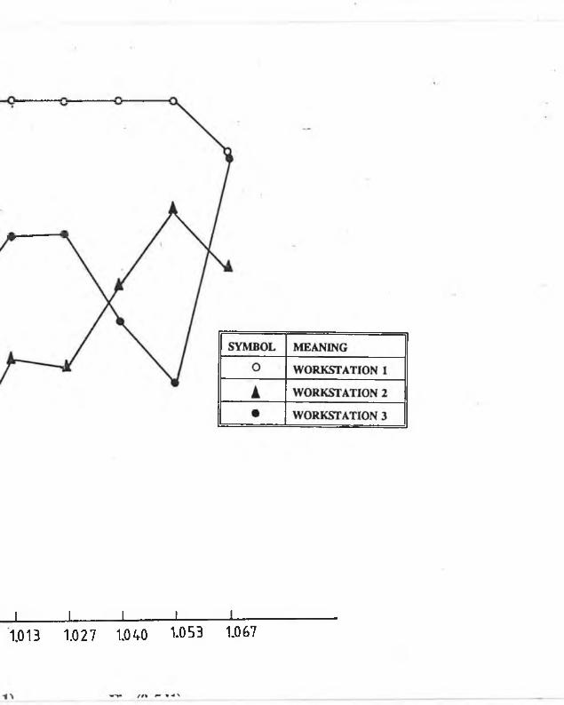
J ________I________I________1________I—1.013 1.027 1.040 1.053 1.067

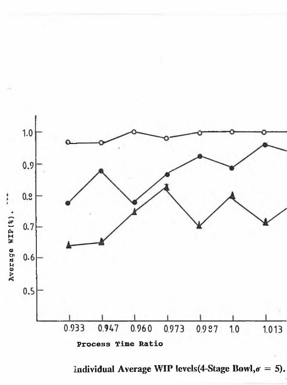
Ave

rage

W

IP(%

P r o c e s s T im e R a t i o

Individual Average WIP levels (4-Stage BowI,<r = 5).

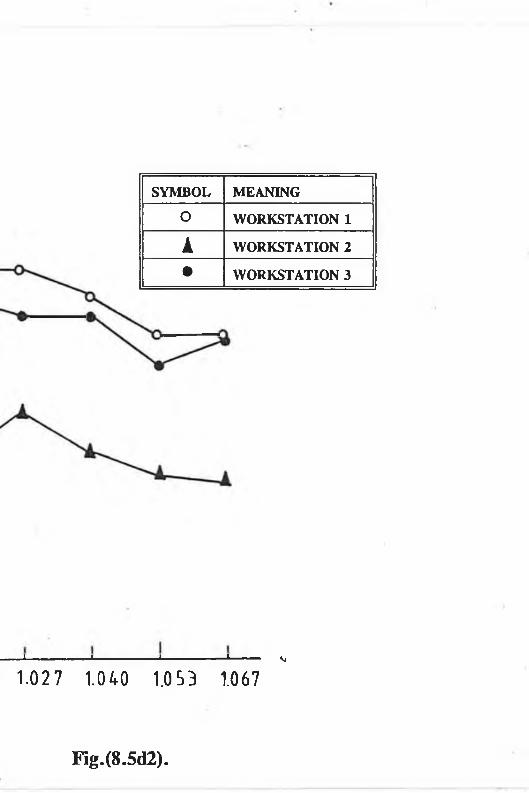
SYMBOL MEANING

O WORKSTATION 1

1 WORKSTATION 2

• WORKSTATION 3

— 1----------------- 1-------------------- 1-------------------»--------- *g

1.027 1.040 1.0 53 1.067

Fig.(8.5d2).

As the variance value increases, the difference in queue lengths before balance are

much less marked, and in fact the respective lengths are much higher at balance. On

passing through the balanced state, it takes a much greater difference in processing

time to reduce the second station’s queue length to zero. The increased variance

effects the third work station the most, preventing it from being reduced to zero.

See Saw

At low values o f processing time ratio, the queue lengths of each of the three stations

are relatively high and tend to follow processing times. The first station, with the

shortest processing time has the shortest queue length, and the third station with the

longest processing time has the longest queue length. Once the system configuration

has passed through balance, the second work station regains its previous queue length,

and the queue length at the third station, -which now has the shortest processing time,

-fades away to zero. The first station now has the longest queue length (Figs. 8 .5b l,

8.5b2).

The introduction of the higher variance value, tends to draw the queue lengths of the

three stations closer together at lower processing time ratios. Once balance has been

achieved however, the length of the queue at the second and third work station fade

away towards zero.

3 Stage Bowl

The bowl configuration produces a much greater range in queue lengths than seen in

either of the previous systems. Irrespective of whether the bowl is concave or

convex, the first station retains the longest queue length. The second station which

has the longest processing time before balance decreases as the bowl becomes more

convex. While this is happening, the queue at the third station which has a shorter

processing time than work station 2 increases in length, and in fact becomes longer

than that at work station 2 before balance is reached. (Figs. 8 .5cl, 8.5c2).

With a concave bowl, the second station, which now has the shortest processing time

also has the shortest queue length, and the third station, the longer queue length. The

concave bowl structure however produces a much smaller range in queue lengths at

individual stations than with the convex structure.

The introduction of the higher variance value, has two noticable effects. Firstly it

brings the queue lengths of stations 2 and 3 much closer together, and reduces the

difference in values obtained with both the concave and convex structure. Secondly

it increases the queue lengths at both stations to much higher values than that

achieved at low variance values. The effect o f variance on the first station is much

less marked.

4 Stage Bowl

The so called 4 stage bowl, effects the first work station in each line in a similar

fashion as the 3 stage bowl, producing a fairly constant queue length of one. The

graphs of the second and third work station queue lengths however are quite different.

With the concave bowl, the second work station has no queue over a large range o f

processing times, while the queue length at work station three is very small but

increasing. Once a queue appears at work station two, both queues continue to

increase in parallel, through the balanced configuration. With the convex structure

however the queue length at work station 3 suddenly drops off, and is overtaken by

the queue at work station 2. (Figs. 8 .5d l, 8.5d2).

The introduction of the higher variance value, has a similar effect to that exhibited

with the three stage bowl, in that it raises the overall queue length at stations 2 and

3, across the range processing time ratio, and brings the queues much closer together.

Effect of Processing Time Variability on Individual Resource Utilisation

The individual resource utilization graph, demonstrates the variation in, the

percentage of overall shift time that a particular resource spend in use, as the

processing time ratio increases.

The see-saw and cantilever configurations demonstrate a distinct tendency at each

work station for utilization values to follow WIP levels at that station. The two bowl

like configurations however would appear to allow the stations to take their respective

utilization values from their postions in the feeder line.

Cantilever

The graph shows that with the cantilever configuration, resource utilization is fairly

linear, both before and after balance. When the processing time at work station one

is relatively low, as so to is the level of inventory in the input buffer, the actual

resource utilization is also low. However as the processing time increases so to does

the utilization and input inventory level. Work stations two and three, with similar

processing time and higher levels of inventory in their buffers, have higher utilization

values, although once the balanced configuration is achieved, and their inventory

levels drop, due to longer processing times at work station one. Their utilization

levels drop fairly linearly with the increase in processing time, while the first work

station remains at maximum utilization.

An increase in the variance value does not redefine the shape of the graph. It does

shift the points at which the first station achieves maximum utilization, and the

utilization values o f work stations two and three to the right, which means that they

now occur at higher processing time ratios. This effect echoes that which is exhibited

in the queue length graphs. (Figs 8 .5a l, 8.5a2).

See Saw

The utilization graphs o f the see saw configuration are also fairly linear about the

balanced state.

The first and third stations show a similar pattern to that exhibited in the cantilever

case, with the first station increasing to maximum utilization as the processing time

increases, and the third station decreasing in a similar fashion. The graph shows

n i

Ave

rage

R

esou

rce

Uti

liz

ati

on

(%1.0

o

0.6

0.4

1 _L X 1 ±0.33 0.46 0.60

P r o c e s s T im e R a t i o

0.7 3 0.86 1.0 1.13 1.26 1.40 1.53 1.66

Individual Average Resource UtiIization(CantiIever,<r = 1). Fig.(8.6al).

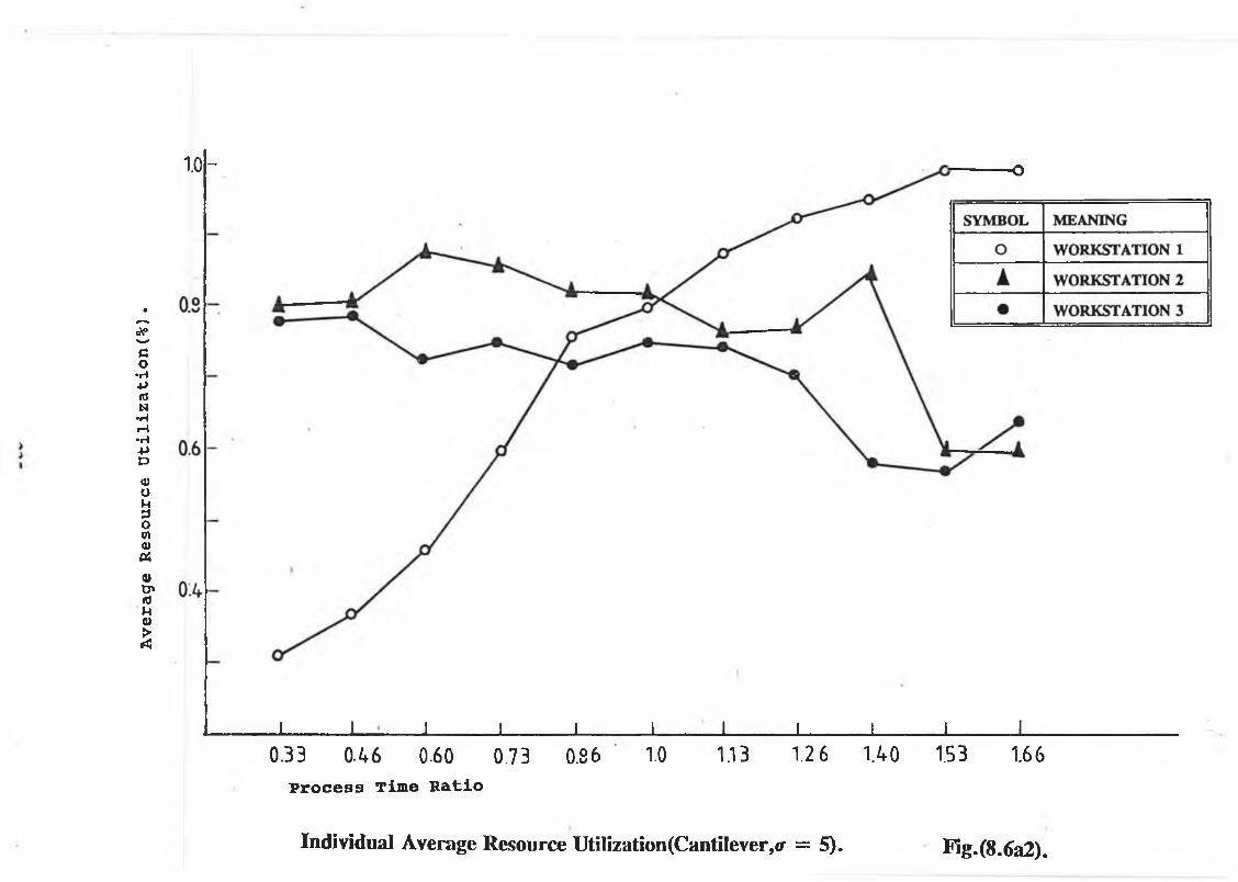
Ave

rage

R

esou

rce

Uti

liz

ati

on

(%).

1 .0 - o

J ________I__ I________ I________ I________ I l________ I________ I________ I________ I__0.33 0.46 0.60 0.73 0.86 1.0 1.13 1.2 6 U 0 1.53 1.66

P r o c e s s T im e R a t i o

Individual Average Resource Utilization(Cantilever,<r = 5). Fig.(8.6a2).

Ave

rage

R

esou

rce

Uti

liz

ati

on

(%).

0 I_______ I_______ I_______ 1_______ I-----------1---------- 1-------0.33 0 46 0.60 0.73 0 86 1.0 1.1 B

P r o c e s s Time R a t io

I n d iv id u a l A v e r a g e R e s o u r c e U t i l iz a t io n ( S e e - S a w „ ir =

SYMBOL MEANINGO WORKSTATION 1

k WORKSTATION 2• WORKSTATION 3

Individual Average Resource UtiIization(See-Saw,<r

Process Time Ratio

SYMBOL MEANINGO WORKSTATION 1

▲ WORKSTATION 2

• WORKSTATION 3

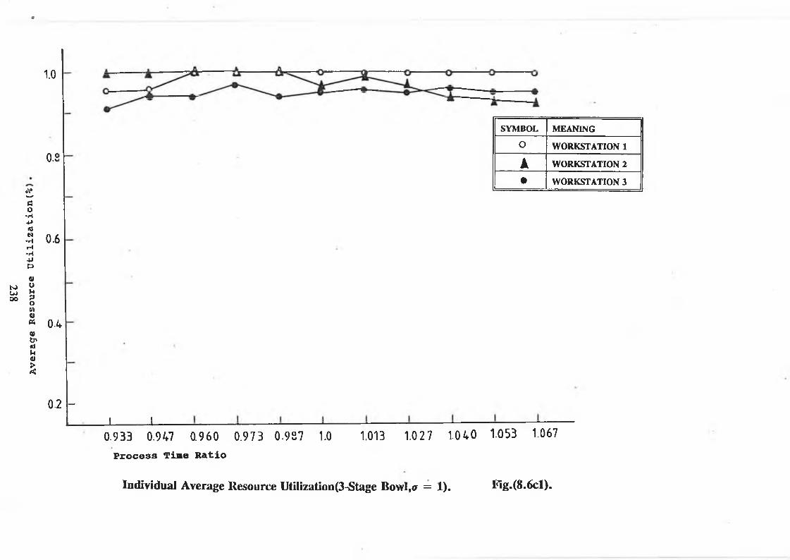
%£Z

Ave

rage

R

esou

rce

Uti

liz

ati

on

(%-0

1.0

o.i

SYMBOL MEANINGO WORKSTATION 1

▲ WORKSTATION 2• WORKSTATION 3

0.6

0.4

0.2 -

i X0.933 0.947 0.960 0.973 0.987

P r o c e s s Tim e R a t io

1.0 1.013 1.027 1.040 1-053 1.067

I n d iv id u a l A v e r a g e R e s o u r c e U t i l i z a t io n ( 3 - S t a g e B o w l , a = 1 ) . F i g . ( 8 . 6 c l ) .

1.0

U>'O

0.8

oV>

'ao

•H+>«JN■rt»—I•H-P»a)oM3o(Aa>tfa>O'idMa)>rt

SYMBOL MEANINGO WORKSTATION 1

A WORKSTATION 2• WORKSTATION 3

0.6

0.4

0.2i

0.933 0.947 0.960 0.973 0.987 1.0 1.013 1.027 1.040 1.0S3 1.067

P r o c e s s T im e R a t i o

Individual Average Resource Utilization(3-Stage Bowl,a = 5). Fig.(8.6c2).

Ave

rage

R

esou

rce

Uti

liz

ati

on

(

P r o c e s s T im e R a t i o

SYMBOL MEANING

O WORKSTATION 1

A WORKSTATION 2

• WORKSTATION 3

J---------1______ I ' l l1.0 1.013 1.027 1.040 1.053 1.067

Ave

rage

R

esou

rce

Uti

liz

ati

on

(o\°

0.9

olì

0.7

0.6

0.5

1.0

SYMBOL MEANING

O WORKSTATION 1

▲ WORKSTATION 2

• WORKSTATION 3

0.933 0.947 0.960 0.97 3 0.98 7 1.0

P r o c e s s T im e R a t i o.01 3 1.027 1.04-0 1.0S3 1.067

Individual Average Resource Utilization (4-Stage Bowl,a = 5).Fig.(8.6d2).

however, that once balance has been achieved, and the processing time at the third

station, reduces, the rate at which utilization drops o f is much greater, than with the

cantilever case, due to the cumulative effect o f the previous stations increase in

processing time and its own reduction. The graph also demonstrates the extent to

which the second station, - which has a constant processing time - is dependant upon

the first. As the processing time ratio increases, the utilization of the second resource

increases although at a slightly slower rate than that o f the first. Once balance is

achieved however, and the processing time at work station one rises above that of

work station two, the utilization value begins to drop off, fairly symmetrically about

the balanced state. A similar symmetry is seen in the queue length graph. (Figs.

8.6b l, 8.6b2).

An increase in the variance value, produces almost the same effect as that seen in the

cantilever case.

3 Stage Bowl

Although the 3 stage bowl produces a large range in queue length, during its concave

state, the actual utilization o f each o f the resources is fairly constant. The sudden

drop off in utilization values see in both the see saw and cantilever case is absent.

Utilization values, would appear to be dictated to by their position in the line, and not

by actual work in progress. Work station one has the greatest utilization value,

followed by two and three respectively, the change from a concave to convex system

would not appear to affect this.

The introduction of higher variance values tends to both reduce the utilization figures

of each and every resource and introduce a greater variability at each resource. A

wider range of utilization values are also produced, although individual utilization

values would still appear to be dictated to by their positions in the line (Figs. 8 .6 c l,

8.6c2).

4 Stane Bowl

2 4 7

The 4 stage bowl graphs are rather similar to that o f the three stage bowl in that they

are farily linear, utilization values tend to follow position in the line, and also for the

most part are concentrated in the same small range. However when stations 2and 3,

are at there greatest processing time values, a sudden drop off in utilization values o f

all three stations is seen. The introduction o f the higher variance value, again tends

to increase the range of utilization values and decrease the linearity of the graph, but

also destroys the rapid decrease in utilization, seen at high values o f processing time

ratio, at the lower variance value. (Figs. 8 .6d l, 8.6d2).

Effects of Processing Time Variability on O verall W ork in Progress and Resource

Utilization

The general trends of both overall utilization, and overall WIP values in the see saw

and cantilever case would appear to be similar. Utilization graphs are convex, the

higher the variance value the flatter the curve, and overall WIP curves, are a distorted

2 shape, with the smaller variance value, producing the greatest WIP range, and the

lowest WIP levels. In contrast, the bowl graphs 'are fairly linear in shape, again

however the smaller variance value produces the greatest utilization, and the smallest

work in progress. In utilization and overall WIP terms therefore it is possible to say

that an increase in the variance of either a cantilever or see saw configurations tends

to bring the system more in tune with a bowl like configuration. Production rate and

cycle time however are not similarly effected.

Cantilever

The shape of the overall resource utilization and work in progress for the cantilever

case, are farily similar to that of the see saw configuration. The utilization curves

are fairly convex, taking their shape from all three stations on the line, although as

the value of variance increases the curves become flatter.

As far as the WIP curves are concerned it is stations 2 and 3 which are the

predominant influence, with the overall WIP curves following the general trends set

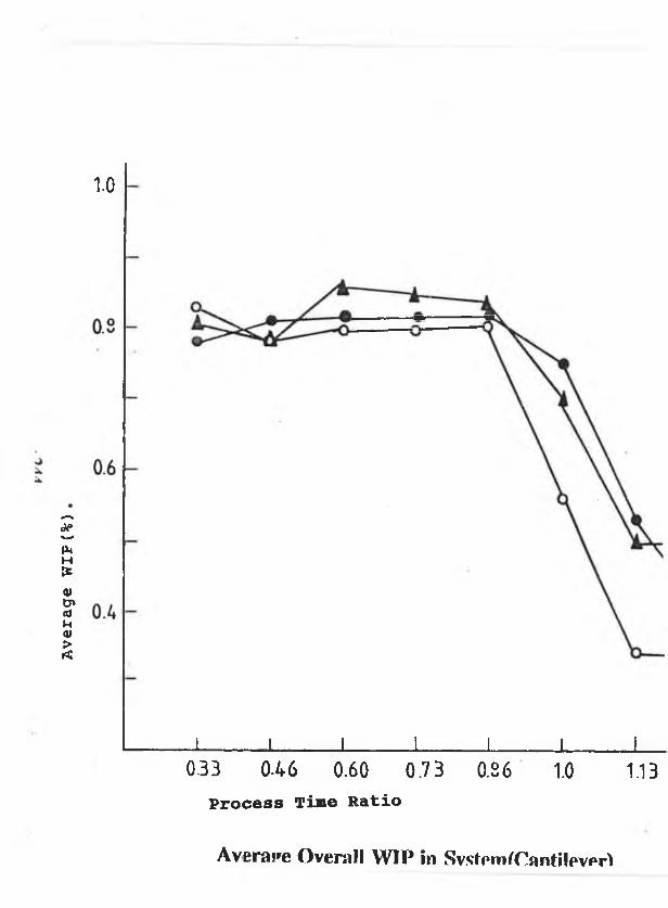
Ave

rage

W

IF(%

)

1.0

J I I l I I I__0.33 0-46 0.60 0.73 0.36 1.0 1.13

P r o c e s s T im e R a t i o

Average Overall W IP in SystemfCantilev#^

SYMBOL MEANINGO » = 1

▲ # = 3

• * = 5

Ave

rage

R

esou

rce

Uti

liz

ati

on

(%).

P r o c e s s T im e R a t i o

Average Overall Resource Utilization(cantilever).

SYM BOL M EANING

O 0 = 1

À # = 3

• 0 = S

1.26 U O 1.53 1.66

Fîg.(8.7a2)

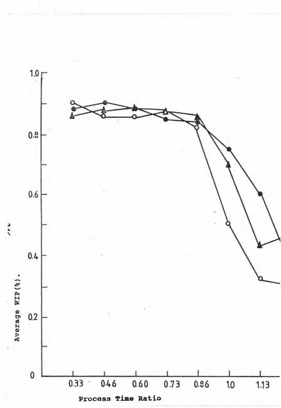
P r o c e s s Tim e R a t io

SYMBOL MEANINGO 0 = 1

Á • = 3• 0 = 5

J I I I__1.26 1.40 1.53 1.66

Average Overall Resource UtiIization(See-Saw). F1g.(8.7b2)

Ave

rage

W

IP(%

1.0

0.9

SYMBOL MEANING

O 0 = 1

▲ 0 = 3

• 0 = 5

0.8

0.7

0.6

0.5

J_ 1 I _L0.93B 0.947 0.960

P r o c e s s T im e R a t i o

0.973 0.987 1.0 1.01 3 1.027 1.040 1.053 1.067

Average Overall WIP in System (3-Stage Bowl). Fig.(8.7cl).

i i I I I L0933 0.947 0.960 0.973 0.937 1.0

P r o c e s s T im e R a t i o

J___1.013

Average Overall Resource Utilization (3-Stage Bowl).

SYMBOL MEANINGO # = 1

▲ » = 3• 0 = 5

0 933 0.947 0.96 0 0.973 0.987 1.0 1 013P r o c e s s T im e R a t i o

Average Overall WIP in System (4-Stage Bowl).

SYMBOL MEANINGO 0 = 1

k 0 = 3• 0 = 5

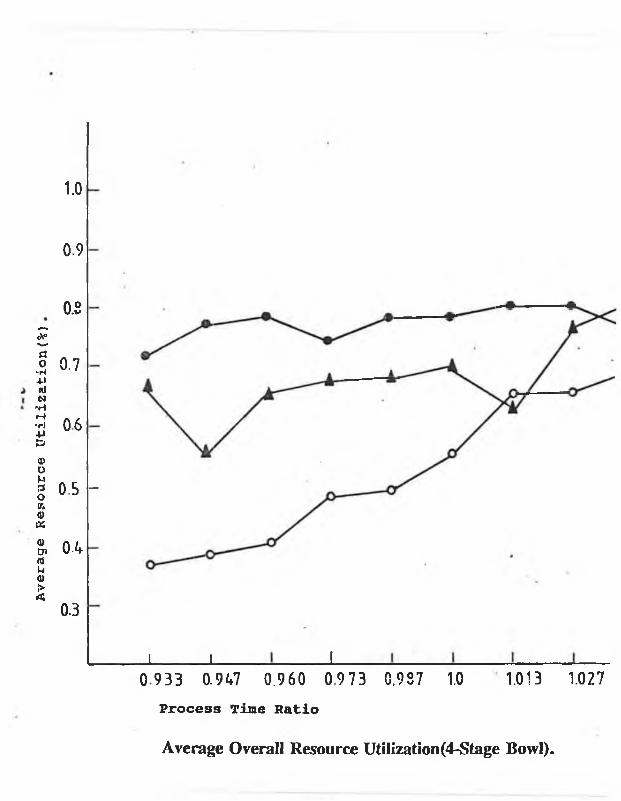
Ave

rage

R

esou

rce

Uti

liz

ati

on

(%)

1.0

0.9

0.8

0.7

06

OS -

0.4

0.3

_L _L 10 933 0.947 0.960 0.9 73 0.9S7 1.0 1.013 1.027

Process Time Ratio

Average Overall Resource Utilization (4-Stage Bowl).

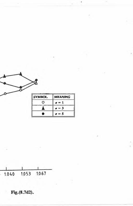
SYMBOL MEANINGO 0 = 1

Á » = 3• » = 5

by these stations. The smaller variance values tend to produce the greatest range o f

WIP values. Before balance is achieved, the overall WIP level is fairly constant,

although utilization figures are increasing having passed through the balanced state,

utilization values begin to decrease slowly while WIP levels decrease at a faster rate,

reaching a steady state quite quickly (Figs. 8 .7 a l, 8.7a2).

S e e S a wThe overall percentage resource utilization, and overall work in progress levels for

the see saw case are shown in Figs (5b 1, 5b2) respectively. For all three variance

levels it is interesting to see that in the utilization graphs, the cantilever effect on

stations 1, and 3 which are opposite, but fairly equal tend to cancel each other out,

allowing the overall graph to mirror the shape o f work station two. The graph shows

that for each level of variance, utilization values are fairly symmetric about balance,

and the- higher the variance value the higher the utilization value. (Fig. 8 .7b l,

8.7b2). The overall WIP level in the system, can also be compared to that o f an

individual station, in this case work station three, because after balance, the extremes

of station, 1 and 2 tend to cancel each other out.

The relationship, between the two graphs is interesting. Before balance, when the

processing time at work station one is approaching that o f the other two stations the

level o f WIP is reducing as the utilization is increasing. Once balance has been

achieved, and the processing time of station one is still increasing, the overall

utilization redues and so to does the WIP level.

3 S t a g e a n d 4 S t a g e B o w lThe three and four stage bowl overall utilization graphs, show no particular deviations

from the individual work station graphs. The higher the variance value, the lower

the utilization and the higher the overall WIP level.

With the 3 stage bowl, the overall WIP and utilization values increase as the

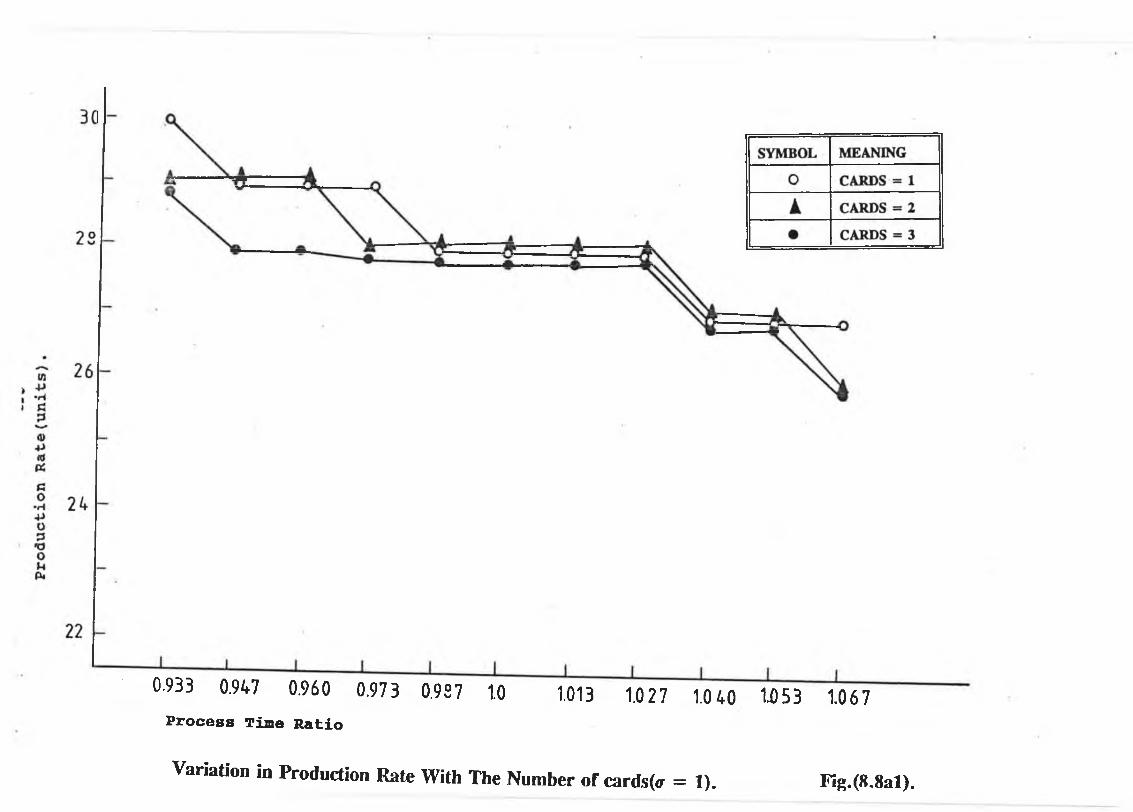
0.933 0.947 0.960 0.973 0.987 1.0 1.013 1.027 1.040 U )53 1.067P r o c e s s T im e R a t i o

Variation in Production Rate With The Number of cards(<r = 1). Fig.(8.8al).

Pro

du

ctio

n

Ra

te(u

nit

s)

30

28

26

24

22_L _L _L

0.933 0.947 0.960Process Time Ratio

¿973 0.987 1.0 1.01.3 1027 1.040 1.053 1.067

Variation in Production Rate With The Number of Cards(cr = 3). Fig.(8.8a2).

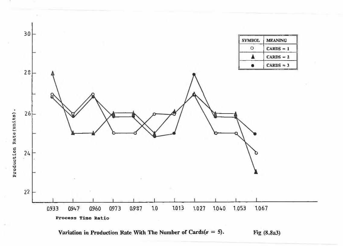
Pro

du

ctio

n

Ra

te(u

nit

s)

30

o

26

24

SYMBOL MEANING

O CARDS = 1

À CARDS = 2

• CARDS = 3

22

1 ± 1 1

0333 m r 0.960 0.973Process Time Ratio

0.987 1.0 1.013 1027 m o 1.053 1067

Variation in Production Rate With The Number of Cards(<r — 5). Fig (8.8a3)

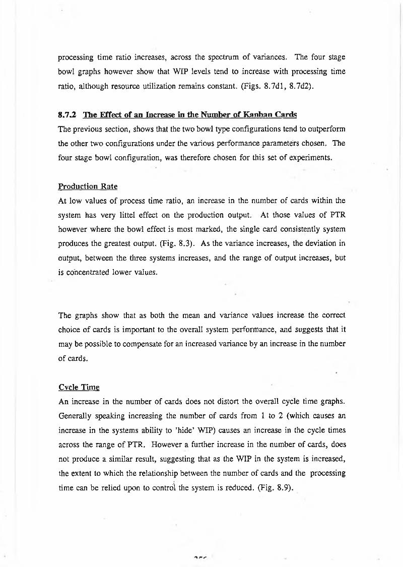
processing time ratio increases, across the spectrum o f variances. The four stage

bowl graphs however show that WIP levels tend to increase with processing time

ratio, although resource utilization remains constant. (Figs. 8 .7 d l, 8.7d2).

8.7.2 Hie Effect of an Increase in the Number of Kanban Cards

The previous section, shows that the two bowl type configurations tend to outperform

the other two configurations under the various performance parameters chosen. The

four stage bowl configuration, was therefore chosen for this set o f experiments.

Production Rate

At low values o f process time ratio, an increase in the number of cards within the

system has very littel effect on the production output. At those values o f PTR

however where the bowl effect is most marked, the single card consistently system

produces the greatest output. (Fig. 8.3). As the variance increases, the deviation in

output, between the three systems increases, and the range of output increases, but

is concentrated lower values.

The graphs show that as both the mean and variance values increase the correct

choice o f cards is important to the overall system performance, and suggests that it

may be possible to compensate for an increased variance by an increase in the number

of cards.

Cvcle Time

An increase in the number of cards does not distort the overall cycle time graphs.

Generally speaking increasing the number o f cards from 1 to 2 (which causes an

increase in the systems ability to ’hide’ WIP) causes an increase in the cycle times

across the range o f PTR. However a further increase in the number o f cards, does

not produce a similar result, suggesting that as the WIP in the system is increased,

the extent to which the relationship between the number of cards and the processing

time can be relied upon to control the system is reduced. (Fig. 8.9).

1 I I _ J I I_ _ _0.933 0.947 0.960 0.973 0.927 1.0 1.013 1.027

P r o c e s s Time R a t io

Variation in Cycle Time with the Number of Cards(<r = 1).

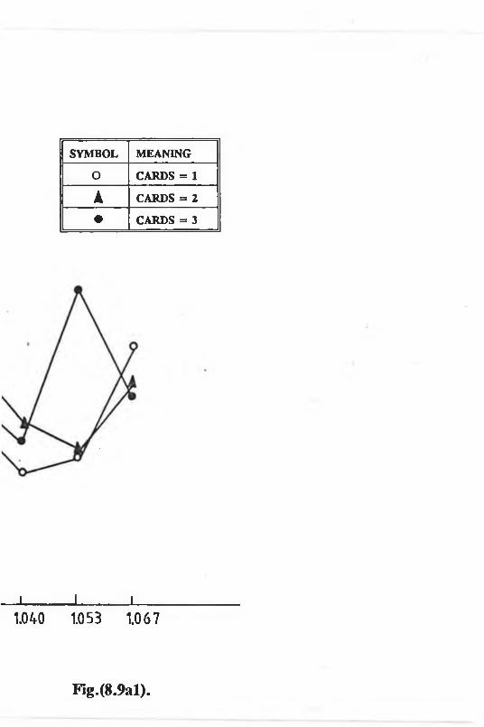
SYMBOL MEANING

O CARDS = 1

▲ CARDS = 2• CARDS = 3

J _______ I_______ I____1.040 1.053 1.067

Fig.(8.9al).

Cyc

le

Tim

e (m

in

2 0 0

180

160n©

K O

120

V a r i a t i o n i n C y c ï e T i m e w i t h t h e N u m b e r o f C a r d s ( < r

I , .1 I I I I I___0.933 0.947 0.960 0.973 0.987 1.0 1013

P r o c e s s Time R a t io

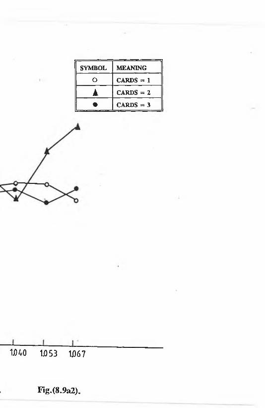
SYMBOL MEANING

O CARDS = 1

À CARDS = 2

• CARDS = 3

1.040 1.053 1.067

Fig.(8.9a2).

J 1 I I I I _ J I____0933 0.947 0-960 0.97 3 0.987 1-0 1.013 1.0 27

P r o c e s s Time R a t io

Variation in Cycle Time with the Number of Cards(<r =5).

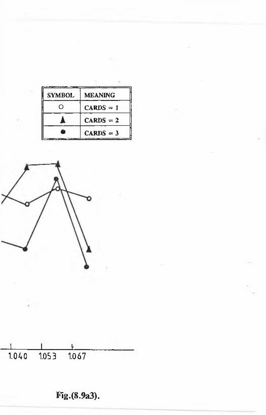
SYMBOL MEANINGO CARDS = 1

▲ CARDS = 2• CARDS = 3

J I k__1.040 1.053 1.067

Fig.(8.9a3).

SYMBOL MEANING

O CARDS = 1

▲ CARDS = 2

• CARDS = 3

i 1 . 1 I 1 1_______________1_______________ I_______________I_______________I_______________ I________.933 .947 .960 .973 .987 1.0 1.013 1.027 1.040 1.053 1.067

P r o c e s s T im e R a t i o

Variation in Overall WIP with the Number of Cards(<r = 1). Fig.(8.10al).

Ave

rage

W

IP(%

)

V a r i a t i o n i n O v e r a l l W I P w i t h t h e N u m b e r o f C a r d s ( < r

SYMBOL MEANING

O CARDS = 1

À CARDS = 2

• CARDS = 3

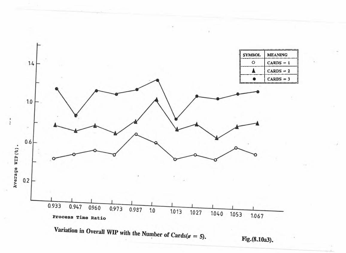
SYMBOL MEANING

O CARDS = 1

i CARDS = 2

• CARDS = 3

Meaning.symbol.

J LJ i I I________1________I________ I________I____________________________0.33 0.46 0.60 0.73 0.S6 1.00 1.13 1.26 1-40 1.53 1.67P r o c e s s T im e R a t i o

V a r i a t i o n i n P r o d u c t i o n R a t e W i t h F i n a l A s s e m b l y V a r i a b i l i t y . F i g . ( 8 . 1 1 ) .

Total WIP

As stated previously, increasing the num ber o f cards, w ithin a system, increases the

allow able W IP within the system . T herefore a production system with 2 K anban

cards per station may have an average o f two units p e r station. Figs. (7.9) how ever

show that across the spectrum o f PTR values, increasing the num ber o f cards to 2 and

3, rarely causes the average level o f w ork in progress to rise above 1. As the

variance increases how ever, the level o f w ork in progress does begin to increase at

higher PT R values. This increase is caused by the processed units spending m ore

tim e in the output buffer. A t low values o f variance and mean processing time, a part

spends little or no time w aiting to be moved to the next station. (Fig. 8.10).

R esource utilization values, show very little deviation as the num ber o f cards are

increased.

8.7.3 The Effect of an Increase in Final Assembly Variability

These experim ents w ere carried out varying the processing time at final assem bly

alone, the system was operating with only one set o f kanban cards per station.

Production Rate

Fig (8.11) shows the effect o f variability at final assem bly for the the three variance

values. W hen the final assem bly processing times are less than that o f the other

stations, very little change in system output occurs. H ow ever as soon as the balanced

configuration has been passed the system output drops o f sleeply, w ith quite sm all

changes in processsing time. T he actual variance value, only has a slight effect on

output.

T he graph suggests therefore, that final assem bly processing time should never rise

above that o f other w ork stations in the line.

Cycle Time

The relationship between cycle time and production rate is emphasised by the final

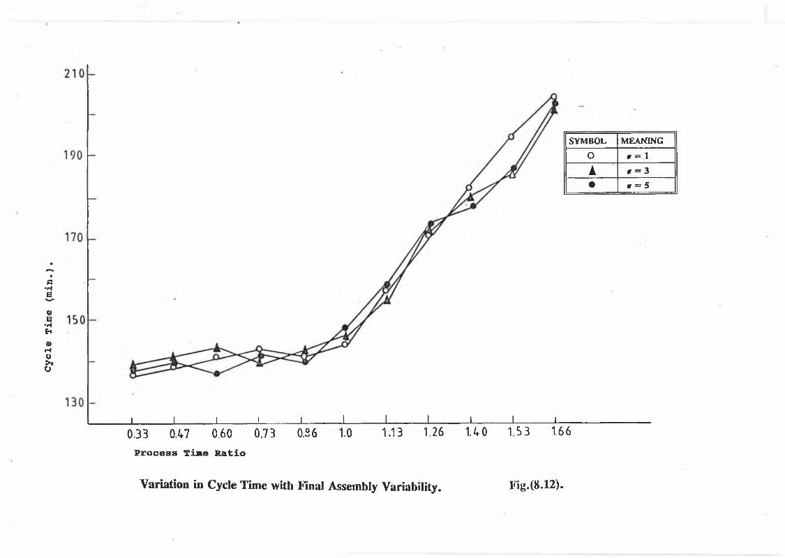
Cyc

le

Tim

e (m

in.)

SYMBOL MEANINGO » = 1▲ # = 3• • = 5

J ________ 1________ I________ i I________ I________ I________ I________ I________ I________ I___0.33 0.47 0.60 0.73 0.S6 1.0 1.13 1.26 1.40 1.53 1.66

P r o c e s s Tima R a t io

Variation in Cycle Time with Final Assembly Variability. Fig.(8.12).

20

18

16

14

1 2

10

O

6

4

2

00.33 0.47 0.60 0.73 0l 36 1.0 1.13 1.26

P r o c e s s T in e R a t io

V í i m f i n n in W « ; t *T'-•»>- <«;<). A i n , , ^7.%-: .»

SYMBOL MEANINGO 0 = 1k 0 = 3

• 0 = 5

Ave

rage

1.0

3.2

0.6

0.4

0.2

_L JL0.33 0.46 0.60 0.73

P r o c e s s Time R a t io

0.S6 1.0 1.13 1.26

V a r i a t i o n i n O v e r a l l W I P w i t h F i n a l A s s e m b l y V a r i a b i l i t y .

SYMBOL MEANING0 # = 1▲ 0 = 3

• 0 = 5

assem bly graphs. A t low values o f PTR , the production rate is very high, and the

cycle tim e very low as the PT R value increases beyond the balanced state, the cycle

tim es increase, as the production rate drops off. A gain the actual variance value has

very little effect on the rate o f change o f cycle tim es and production rate. (Fig.

8 .12). N otice that the w ait time at final assem bly follow s cycle tim e (Fig. 8 .13).

Total System WIP

T he sudden change in the perform ance o f both graphs how ever coincides w ith a

sudden increase in the W IP in the system, as the PT R value passes through balance.

(See F ig . 7 .12). T he average W IP in the input buffer begins to increase, and the

output buffer, which has previously been used only as a transitionary point, is now

being used as an actual storage facility. Once W IP appears in the output buffer, the

average W IP held increases at a sim ilar rate to the increase in the input buffer, but

at m uch low er values.

An increase in variance values has very little effect in the perform ance o f either input

or output buffers.

8 . 8 D I S C U S S I O N / C O N C L U S I O N SBlocking is said to occur w ithin a manufacturing system , when a succeeding buffer

is full. C onversely starving may occur when a preceding buffer is em pty. T herefore

it may be concluded that the first station in a line can never be starved o f parts and

the final station in a line can never be blocked. Interm ediary stations how ever may

be both blocked and starved causing the greatest effect at the adjacent stations. I f a

particular w ork station is blocked, the operation o f the line may be split into two

distinct segments by the blocked w ork station. P rocessing continues at all preceding

w ork stations, until each o f them is blocked. (The adjacent station being block first).

Processing continues at succeeding stations until each is successively starved.

'»/TO

Section (8 .7 .1 ) exam ines various system configurations. G raphs (8 .5), show the

effects o f these configurations at the W IP levels at various w ork stations in an

assembly line.

The cantilever case graphs (Fig. 8.3a) show that as the processing tim e for the first

station increases, a blocking effect, begins to occur, at w ork station and the level o f

W IP increases in this input buffer and reduces in the input buffers o f the o ther two

stations (ie. starved). T he adjacent w ork station how ever experiences the m ost rapid

reduction in W IP level. This increased blocking effect causes a drop o ff in the

production rate (Fig. 8 .4), an increase in cycle time (Fig. 8 .5 ), and a drop o ff in

resource utilizations at w ork stations 2, and 3 as they are starved for parts.

The see saw graphs presented (Figs. 8.5b) can also be explained in term s o f blocking

and starving. At low values o f PTR, the blocking effect o f w ork station 3 tends to

dominate the W IP level at the interm ediary station. Once the balanced position has

been passed through how ever, the level o f W IP at w ork station 2 is now subject to

blocking at w ork station 1 and follows trends in w ork station 1. T he last w ork station

in the line, how ever, is now subject to the com bined blocking effect o f w ork stations

2 and 1, and the W IP level drops o ff com pletely.

The symmetry o f each o f the see saw graphs (Figs. 8 .3b, 8 .4b, 8 .5b) tend to agree

with the conjecture o f H illier and Boling (see Silver et al) that the optim al allocation

o f processing tim e is sym m etric,- and blocking at the beginning o f a line, causes a

similar variation in perform ance param eters, as starving at the end o f a line.

The bowl graphs dem onstrate that the initial stations are relatively unaffected in these

configurations. A t low values o f PTR , w ork stations 3 is subjected to the blocking

effects o f w ork station 2 , and consequently is starved o f WTP in the input buffer. The

level o f W IP at w ork station 2 decreases slowly as the PTR value increases and all

the processing times align. As the processing times at w ork stations 1, and 3 rise

above that o f w ork station 2, the blocking is eased slightly and the level o f inventory

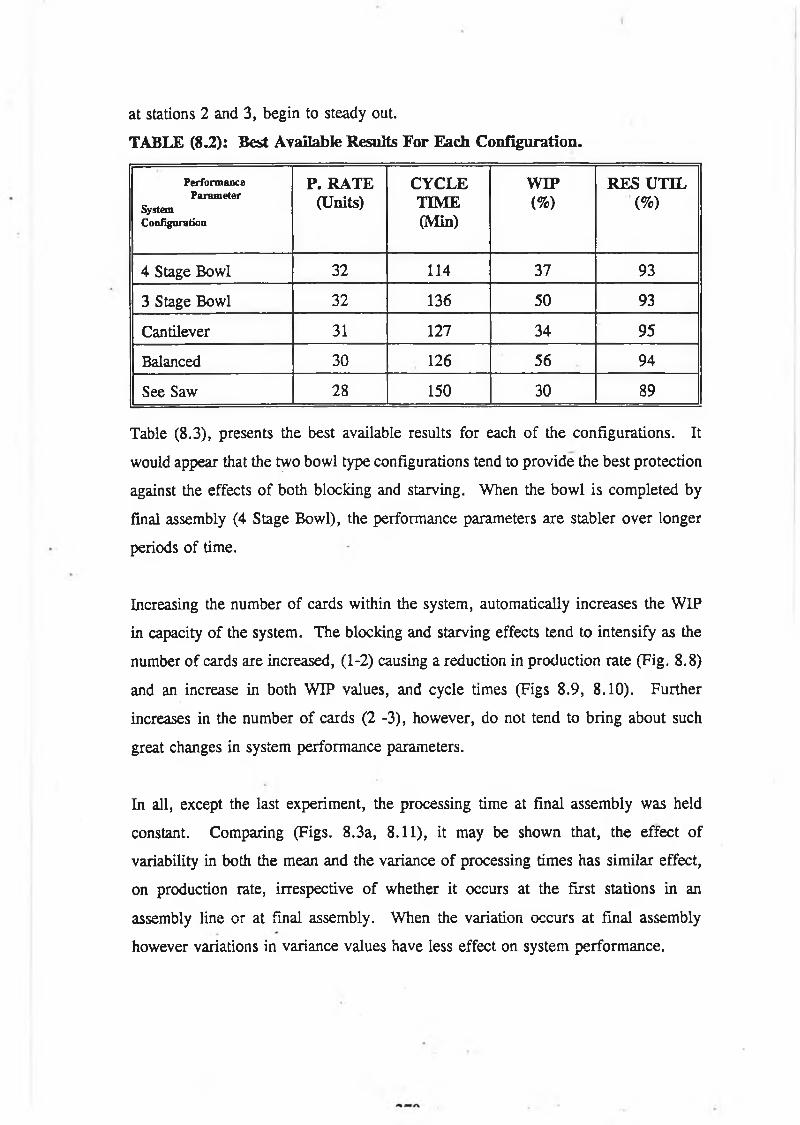
at stations 2 and 3, begin to steady out.

TABLE (8.2): Best Available Results For Each Configuration.

PerformanceParameter

SystemConfiguration

P. RATE (Units)

CYCLETIME(Min)

WIP(%)

RES UTIL (%)

4 Stage Bowl 32 114 37 93

3 Stage Bowl 32 136 50 93

Cantilever 31 127 34 95

Balanced 30 126 56 94

See Saw 28 150 30 89

Table (8 .3), presents the best available results for each o f the configurations. It

would appear that the two bow l type configurations tend to p rovide the best protection

against the effects o f both blocking and starving. W hen the bow l is com pleted by

final assembly (4 Stage Bow l), the perform ance param eters are stabler over longer

periods o f dme.

Increasing the num ber o f cards w ithin the system, autom atically increases the W IP

in capacity o f the system. T he blocking and starving effects tend to intensify as the

number o f cards are increased, (1-2) causing a reduction in production rate (Fig. 8.8)

and an increase in both W IP values, and cycle times (Figs 8 .9 , 8 .10). F u rther

increases in the num ber o f cards (2 -3), how ever, do not tend to bring about such

great changes in system perform ance param eters.

In all, except the last experim ent, the processing time at final assem bly was held

constant. Com paring (Figs. 8 .3a, 8 .11), it may be shown that, the effect o f

variability in both the mean and the variance o f processing times has sim ilar effect,

on production rate, irrespective o f w hether it occurs at the first stations in an

assembly line o r at final assem bly. W hen the variation occurs at final assem bly

however variations in variance values have less effect on system perform ance.

This effect is accenuated while in the balanced configuration. (See F igs. 8 .3a, 8 .11,

8.4a, 8 .12). W IP values are much low er, w hen the variation occurs at final

assem bly, and are much more stable over longer m ean processing tim e spans.

C O N C L U SIO N S

1. D ifferen t system configurations produce quite d ifferent effects in term s o f

system perform ance parameters.

2. Bowl type configurations require much sm aller changes in mean processing

tim es to produce similar effects in perform ance param eters than either o f the

o ther configurations. Bowl configurations also produce the greatest changes

in perform ance parameters above the balanced case.

3. The balanced configuration does not always produce the m ost efficient results,

in term s o f production output, cycle tim es etc. and m ay be im proved by

unbalancing.

4. The H illier and Boling (See Silver Et Al [ ]), hypotheses on the reversibility

o f processsing systems, is dem onstrated in the set o f "See Saw" configuration

graphs.

5. A t low variance values, the introduction o f extra cards causes little change in

system perform ance param eters as the variance increases how ever the num ber

o f cards becom e increasingly im portant to the effective control o f the system.

6. An increase in variance of processing time, on perform ance param eters are

m uch less im portant at final assembly than at the first station in an assem bly

CHAPTER 9

CONCLUSIONS

9 . 1 S U R V E Y O F I N V E N T O R Y C O N T R O L P O L I C I E SThis thesis presents results on inventory control practises w ithin the Irish E lectronics

Industry. As outlined in the introduction, C hapter 4 presents an overview o f

inventory control policies in use within the industry as determ ined by an industrial

survey. The main characteristics o f these policies are:

1. T he industry is predominantly push orientated.

2. In term s o f control policies, very little difference exists between large

and m edium firm size. Small firms how ever d iffer m arkedly from the

first two.

3. Industry consists mainly o f assembly operations, m ost o f which (93% )

have M RP systems.

4. M R P is loosely applied to cover all levels o f com puterization.

H ow ever the majority o f firm s tend to use M RP m ainly for order

launching. Very few closed loop systems are in operation, and only

tw o ’A ’ class users are in evidence.

5. In basic M RP terms, only two o f the inputs have high levels o f

com puterization - BOM , IR-, the M PS exhibits much low er

com puterization levels.

6. T he m ajority o f firms utilize net change M R P (See C hapter 5). Lot

sizing along with other M RP features play an im portan t role in

requirem ents generation.

7. Levels o f com puterization vary m arkedly between firm s size, with

large firm s having high levels o f com puterization, and sm all firm s

exhibiting low er levels.

8. D ata accuracy is relatively low among M RP elem ents w hich are not

com puterized. Accuracy levels, are low across the spectrum o f firm

size.

272

9. JIT awareness is relatively high (70% ) across the spectrum o f firm

size, but im plem entation tends to be mainly concentrated in the large

to medium size category.

10. JIT im plem entation is concentrated in the JIT delivery area, w ith cross

training o f em ployees and Kanban operation also featuring.

The survey also highlights the problem that although the electronics industry is push

based, M RP has failed to perm eate all levels o f the m anufacturing hierarchy, leaving

many o f the sm aller firm s with very low levels o f com puterization, and integration

among the varied inventory control functions.

In recent years, the em ergence o f JIT onto the Inventory Control scene has heralded

a new departure in inventory managem ent w orldw ide. The survey shows how ever

that it has tended to be the larger firms who have benefited from this new thinking,

with sm aller firm s retaining the older inventory methods.

I f current trends are to change in the future tim e and money m ust be spent on

educating small firm s as to the potential profitability to be gained from a m ove

towards new er inventory control practises.

9 . 2 L O T S I Z I N G W I T H I N M R PThe generation o f requirem ents within M RP is investigated in Chapter 6. The linear

program m ing form o f the M RP m odel; which was developed, and tested under a

variety o f operating conditions, was found to produce optim um requirem ents,

irrespective o f the form o f the product structure. T he m odels’ perform ance was

found to be enhanced by the introduction o f a dynam ic planning horizon outlining the

conditions under which the m odel is run.

The models perform ance was also com pared to requirem ents generated by some o f

the m ore w idely used lot sizing techniques. In all cases the linear program m ing

m odel, outperform ed, each o f the other techniques.

Tw o im portant lessons may be leam t from results presented in this section. F irstly ,

firm s interested in cost reduction may achieve greater benefits by switching to the

linear program m ing model. Secondly, sm aller firm s, frightened by M R P ’s em phasis

on com puterization, and the high levels o f investm ent involved should be m ade to

realize that M RP can be perform ed relatively sim ply and cheaply on standard

m athem atical program m ing packages which can be either purchased o r developed

internally. A ll that is required is an understanding o f the m ore rudam entary aspects

o f M RP.

9 . 3 K A N B A N S I M U L A T I O NSim ulation is an as yet untapped management aid. C hapter 8 investigates the operation

o f a Kanban system through the use o f simulation. The first set o f experim ents w ere

perform ed, w ith a view to investigating the effects o f process tim e im balance on

various system perfom ance param eters. These experim ents show that the balanced

configuration does not always produce the best results in term s o f perform ance

param eters and that by varying process times at individual stations, w ork-in-progress

levels, m achine utilizations and cycle times can be im proved upon. Bowl type

configurations w ere found, not only to provide the best protection against blocking

and starving, (See Chapter 8) but also in dealing w ith effects o f w ork station

variability. The experim ents conducted, also dem onstrated the effect o f near

processing time variability on perform ance param eters.

The second set o f experim ents deals with the im pact o f an increase in the num ber o f

cards w ithin the system. T he results show that an increase in the num ber o f cards,

reduces cycle tim es, and increases W IP values and cycle times. T here com es a point

however, w here the effects o f blocking and starving becom e saturated and further

increases in the num ber o f cards have little effect on param eters.

The final set o f experim ents, examines, the effect o f process tim e variability on final

assembly. Results suggest that once the process time at final assem bly exceeds that

■>■74

at o ther stations, the production rate drops, and therefore should not be allow ed to

drop below the balance value. F inal assembly processing tim e also effects the value

o f W IP in the output buffer, once the processing tim e passes through balance, the

W IP value in the input buffer rises above zero. V arying the processing tim e at o ther

stations does not have such an exagerated effect. F inally , variability in w ork station

mean w ould appear to have a less noticeable effect w hen it occurs at final assem bly,

that at any other w ork station on the line.

In the future, sim ulation m ay play an im portant ro le , in the transfer o f production

systems from push to pull, by allow ing m anagers to forsee the im plications and

results o f changes, and m ake any adjustments necessary.

9 . 4 R E C O M M E N D A T I O N S F O R F U R T H E R W O R K1. The developm ent o f a good branch and bound procedure, to allow the

integration o f non-integer lot size requirem ents w ithin the linear

program m ing m odel.

2. T he introduction o f price break facilities into the M R P model.

3. To conduct a sim ilar set o f sim ulation experim ents over a much greater

num ber o f iterations and for a much larger period to reduce the erro r

m argin.

4. T he com parison o f Push and Pull type system s, perform ance over a

sim ilar range o f process tim e ratios.

5. T he developm ent o f a com plete JIT m odel, w ith a user interface so

that inexperienced sim ulators can pick pertinent data from a menu

system.

R E F E R E N C E S1. Zangw ill W .; A backlogging m odel and m ulti-echelon m odel o f a dynam ic

enconom ic lo t size production system - a net w ork approcah. M gm t. Sci.

V ol. 15 N o. 9, 1969.

2. ■ Love S .; A facilities in series inventory m odel w ith nested schedules. M gm t.

Sci. Vol. 18 N o. 5, 1972.

3. N ew C .; Lot Sizing in m ulti-level requirem ents planning system. PIM (4th

Q uarter 1974).

4. Gavish Br, A fentakis P . , and K arm arkar V ., Com putationally efficient optim al

solutions to the Lot Sizing problem in m ultistage assem bly systems M gm t. Sci

V ol. 30 N o. 2, 1984.

5. B row ne J ., H arhen J ., Shivnan J .; Production M anagem ent Systems - A CIM

perspective. A ddison W esley 1988.

6. Crow sten W .N ., W agner M .H .; D ynam ic lot size models fo r multi-stage

assem bly systems. M gm t. Sci. Vol. 20 N o .l , 1973.

7. C larke A ., Scarf H .; O ptim al policies for the multi echelon inventory

problem . M gm t. Sci. V ol. 6, N o. 4, 1960.

8. Schw arz L ., Schrage L ., Optim al and system m yopic policies for multi

echelon production and inventory assem bly system s. M gm t. Sci. Vol. 21 No.

11, 1975.

9. D orsey R ., Hodgson T .; A netw ork approach to a m ulti facility m ulti-product

production scheduling problem w ithout backordering. M gm t. Sci. V ol. 21,

N o. 7, 1975.

10. G lover F ., Hultz J ., K lingm an D ., and Stutz J ., G eneralized netw orks, a

fundam ental com puter based planning tool. M gm t. Sci. V ol 24, N o. 12,

1978.

11. G abbay H .; M ulti stage production planning. M gm t. Sci. Vol. 25, Nov.

1979.

12. Steinberg E .; N apier H ., Optim al m ulti-level lot sizing for requirem ents

planning system. M gm t. Sci. Vol 26, N o. 12, 1980.

13. Thom as J .; N ote on S-N M RP M odel Form ulation. M gm t. Sci. Vol. 21,

1975.

14. Blackburn J ., M illen R .A .; Im proved H euristics for M ultistage Requirem ents

P lanning System. M gm t. Sci. Vol. 28, N o. 1, 1982.

15. Z ahorik A ., Thom as J ., T rigeiro W .; N etw ork program m ing m odels for

production scheduling in multi-stage m ulti-item capacitated system . M gm t.

Sci. V ol. 30, No. 3, 1984.

16. Billington P ., M cClain J ., Thom as L .; M athem atical Program m ing

approaches to capacity constrained M RP system s, Review, form ulation and

problem reduction. M gm t. Sci, Vol. 29, No. 10, 1983.

17. H o J ., M cKenny W .; Triangularity o f the basis in linear program s for

m aterial requirem ent planning. OP. Res. Letter. V ol. 7, N o. 1, 1988.

*

777

18. Prentis E. K hum w ala B .; M R P lo t sizing w ith variable production/purchasing

costs: form ulation and solution. Int. J. P rod . Res. Vol. 27, N o. 6, 1989.

19. H uang P ., Rees L ., T ay lor B .; A sim ulation analysis o f the Japanese Just-In-

T im e Technique (with K anbans) fo r a m ultiline m ultistage production system.

AM . Inst. D ec. Sci. V ol 14, 1983.

20. Ebrahim pour M , Fath i B .M .; D ynam ic sim ulation o f a K anban production

inventory system. U O PM . Vol. 5, N o. 5 , 1981.

21. Schroer B .J., Black J .T ., Zhang S .X .; Just-In-T im e with K anban,

M anufacturing system sim ulation on a m icro com puter. Sim ulation Vol. 45,

N o. 2 ,1 9 8 5 .

22. Sarker B .R ., H arris R .D .; T he effect o f im balance in a Just-In-Tim e

production system: A sim ulation study. U O PM . V ol 26, N o. 1, 1988.

23. F a llo n D ., B row ne J ., Sim ulating Just-In-T im e System s, U O P M ., V ol. 8, No.

6, 1987.

24. V illeda R ., D udek R ., Sm ith M .L .; Increasing the production rate o f a Just-

In-Tim e system w ith variable operation tim es. U PR . Vol. 26, N o. 11, 1988.

25. G oldratte E ., Cox J .; T he G oal-excellence in m anufacturing. N orth River

Press, 1986.

26. G roover M .P .; A utom ation, production, system s and com puter integrated

manufacturing 1987. Prentice H all.

27 . Sizer J .; An insight into m anagem ent accounting. Penguin 1985.

in *

28. M easuring the Cost Industrial Com puting. 1985.

29. B urbidge J .L .; T he principles o f production control. M acD onal and Evans,

1978.

30. W ilde R .; Productions and Operations M anagem ent. W iley 1979.

3 L H all R . ; Z ero inventories. Dow Jones-Irw in 1983.

32. O r lic k y J .; M aterial Requirement Planning. M cG raw H ill 1975.

33. Schonberger R .J .; Japanese M anufacturing Techniques. F ree Press 1982.

34. R ice, J. Y oshikawa, T .; A com parison o f K anban and M RP concepts, fo r the

control o f m anufacturing systems PIM 1982.

35. M onden, Y .; Toyota production system: Practical approach to Production

M anagem ent. A tlanta GA 1983.

36. O ’M alley E .; Industry and econom ic developm ent - The Challenge fo r the

Late C om er. Gill and M acM illen, 1989.

37. O ’K eefe B .; E lectronics now big contributor to Irish econom y. Irish T im es,

January 11, 1991.

38. F itzpatrick J ., K elly J .; Perspectives on Irish Industry IM I 1985.

39. C raw ford K ., Blackstone J ., Cox J .; A study o f JIT im plem entation and

operating problem s. HPR. Vol. 26, N o. 9.

40. A nderson J. Schoeder G ., Tupy S .; M aterial requirem ent planning - A study

; o f im plem entation and practise. APICS. 1981.

279

41. Voss C .A ., Robinson; A pplication o f Just-In-T im e m anufacturing techniques

in the U nited K ingdom . U O PM , V ol. 7, N o. 4.

42. Cheng T .; The Just-In-Tim e production: A survey o f its developm ent and

perception in the H ong Kong electronics industry . Int. J. M gm t. Sci. V ol.

16, N o. 1. 1987.

43. N eil G ., O ’M ara J .; Introducing JIT in to a high technology electronics

m anufacturing environm ent. U O PM , V ol. 7, N o. 4.

44. Landy P .; Com peting in the global electronics industry: The challenge for

indigenous Irish firm s. MBS Thesis U C D 1982.

45. H O C .; Evaluating the im pact o f operating environm ents on M RP system

nervousness. U O PM , Vol. 27, N o. 7, 1989.

46. Schonberger R .J .; A pplications o f single-card and dual card K anban.

Interfaces, Vol 13.

47. Schonberger R .J .; W orld class m anufacturing - The lessons o f sim plicity

applied. F ree Press 1986.

48. Berry W ., V ollm ann T ., W hybark D .; M anufacturing planning and control

systems. D ow Jones-1988.

49. Schriber J .; T he nature and role o f sim ulation in the design o f m anufacturing

systems. P roc. W inter Sim. Conf. 1987.

50. D avis D ., Pegden C .; Introduction to SIM A N . P roc. W inter Sim. Conf. 1987.

51. Magazine M. J., Silver G.L.; Heuristics for determing output and work

allocations in series flow lines. UPR. Vol. 16, No. 3, 1978.

52. Carrie A.; Simulation of manufacturing systems. Wiley 1988.

53. MGG User Guide, Version 2.1; Scican Ltd. August 1985.

54. SCICONIC/VM User Guide, Version 1.40; Scican Ltd. February 1986.

55. Pegden D., Shannon R., Sadowski R.; Introduction to Simulation using

SIMAN. McGraw Hill 1990.

56. SIMAN IV Reference Guide. Systems Modelling Corporation 1990.

57. SIMAN IV Environment Reference Guide. Systems Modelling Corporation

1990.

">Q1

MRP and JIT Survey Questionnaire

APPENDIX 1

6. Type of Manufacturing.- (please tick)

a. Assembly ___ b. Fabrication c. Both __

7. Type of Process: (please tick)

a. Job Shop ___ b. Continuous Process c. Assembly I Ine

S. Approximate number of possible "end-ltems" In master schedule (excludingservice parts): ___________________________________________________________________

9. Approximate number of different part, component, and assembly numbers:

10. Number of levels In the Bill of Material: ____________________________________

11. Number of Employees at your Facility: _________________________________________

Part B: Description of MRP System Status

1. What Is the current and planned status of the following MRP systeme lements?(please tick appropriate box)

a. Forecasting End I terns

b. Bill of Materlal

c. Inventory Stock System

d. Master Production Schedule

e. Parts Explosion

f. Order Release

g. Purchasing

h. Capacity Planning (rough cut)

1. Operations Scheduling

J. Shop Floor Control

Current PIanned

i o — otfl 3a a a c

r013c01

I o — oCO 3 cd -a a. c

zCD3C0)

1b

STUDY OF MATERIAL REQUIREMENTS PLANNING SYSTEMS

The questions In this survey are designed to be answered by the Materlals Manager, Production and Inventory Control Manager, or other person who Is most familiar with the MRP system In your company. If you encounter questions which you cannot answer or questions which do not apply to your company, please leave them blank. Answer the remaining questions by entering or circling the most appropriate response. When you have completed the questionnaire, please return It In the prepaid return envelope. Thank you for your help.

Part A; Company Description:

1. Title of Respondent:_____

2. Your Company's Industry:

3. If any please state name of parent plant/company:

4. Please tick product/descrIptIon which most suits your product.

a. Electronic Computers: ___

b. Electro-Mechanical (Indust.):

c. Electro-Mechanical (Consum.):

d. Electronic components.:

5. Type of Products: (please tick)

a. Make-to-Order b. Make-to-Stock c. Both

Which of the following features does your MRP system have? Please circle the correct answer.

a. Update Method:

b. Pegging:

c. Cycle CountIng:

Net Change

Yes

Yes

Régénérât I ve

No

No

d. Automatic lot sizing by computer: Yes No

What Is the accuracy of the following (please circle correct answer)

types of data?

Poor Fa I r Good ExceI Ient

a. Inventcpry Records 1 2 3 4

b. BOM Records 1 2 3 4

c. Market Forecasts 1 2 3 4

d. Master Production Schedule 1 2 3 4

e. Production Lead Times 1 2 3 4

f. Vendor Lead Times 1 1 3 4

g. Shop Floor Control Data 1 2 3 4

h. Capacity Plan 1

How Is the term "MRP" used In your company.

2 3 4

a. In the broad sense, control system.

as a closed-loop manufacturIng

b. In the narrow sense, as parts explosion and order IaunchIng.

c. Other (Please describe)

Part C: MRP Seneflts and Costs:

1. To what degree have the following benefits been achieved from your MRP system, (please circle correct answer)

Degree of Improvement

a. Improved customer satisfaction

b. Better production scheduling

c. Improved manufacturing lead11 mes

Little/None Some Much

3

3

3

Very Much

4

4

4

d.. Better control Inventory

l c

t

1. To what, extent have you encountered the following types of problems with data accuracy, availability, or format, In Implementing your MRP system? (please circle correct answer)

P art D: Implementation Problems:

Degree of ProblemLittle/None Some Much

a . Master production schedule 1 2 3

b. Production lead times 1 2 3

c. Lack of suitability of software 1 2 3

d. Constraint of computer hardware 1 2 3

e. Lack of company expertise In MRP 1 . 2 3

f . High cost of the MRP system 1 2 3

What; Is the major problem your firm has faced In Imp IementIng

Part E: Implementation Approach Used:

l. To what extent were the following sources of expertise and Information used regarding MRP? (please circle correct answer)

Little/None Some Much

VeryMuch

a. Consultants 1 2 3 4

b. Computer manufacturers 1 2 3 4

c. Software vendors 1 2 3 4

d. Books or periodicals 1 2 3 4

What was the source of software for your MRP system? (P lease tick)

a. ___ Vendor supplied with: (I) _ mod IfIcatIon (II D __ No mod If I

b. ___ Developed InternalJy

1 ^

Part F:

1. Do you think J.I.T. may be applied successfully In your manufacturing environment, (please tick)

a. Yes b. No

2. Have you Implemented any aspects of J.I.T.

a. Yes b. No

3. If yes: What elements: (please tick)

a. _______ Reduce set-ups

b. Group technology

c. _______ T.P.M. program

d. _______ Cross training employees

e. _______ Kanban

f. _______ J.I.T. delivery/purchasing

g. _______ Uniform work loads

h. _______ Zero defects/quality circles

4. If No: Do you Intend to In the future.

a . Yes b . No

5. If Yes: (please tick elements) a. __ b. c. d. e.

f. g. h.

l e

IJNPROG 2 MRP Model Input and Results

APPENDIX 2

M I N4 0 P 1 1 + 1 0 P 1 2 + 5 P 1 3 + 1 P 1 4 + 2 1 1 1 + 2 1 1 2 + 2 1 1 3 + 2 1 1 4 + 4 0 P 2 1 + 1 0 P 2 2 + 5 P 2 3 + 2 + 2 I 2 4 + 4 0 P 3 1 + 1 0 P 3 2 + 5 P 3 3 + 2 I 3 1 + 2 I 3 2 + 2 I 3 3 + 2 I 3 4 + 4 0 P 4 1 + 1 0 P 4 2 + 2 I 4 1 + + 2 1 5 1

- I 2 1 + P 2 1 - 2 P 1 1 = 0I 2 1 - I 2 2 + P 2 2 - 2 P 1 2 = 0I 2 2 + P 2 3 - 2 P 1 3 = 0- I 3 1 + P 3 1 - 3 P 1 1 = 01 3 1 —I 3 2 + P 3 2 - 3 P 1 2 = 0I 3 2 + P 3 3 - 3 P 1 3 = 0- 1 4 1 + ' P 4 1 —2 P 3 1 = 0I 4 1 + P 4 2 - 2 P 3 2 = 0- I 5 1 + P 5 1 - P 3 1 = 0I 5 1 + P 5 2 - P 3 2 = 0P 4 1 + P 4 1 = 2 4P 3 1 + P 3 2 + P 3 3 = 1 2P 2 1 + P 2 2 + P 2 3 = SP l l + P 1 2 + P 1 3 + P 1 4 = 4p=¡l¿p = o= ^2C E O B ]

- I 1 1 + P 1 1 = 11 1 1 - I 1 2 + P 1 2 = 11 1 2 - 1 1 3 + P 1 3 = 1 I 1 3 + P 1 4 = l

" P E R I O D O N E "" P E R I O D T WO " " P E R I O D T H R E E

" P E R I O D F O U R "

O B J . F U P R I M A L

O P T I M A L S O L U T I O N 1 5 2 0 . 0 0 0 0

S O L U T I O N D U A L S O L U T I O NP l l P 12 P 1 3 1 1 3 P 2 1 P 2 2 P 2 3 P 3 1 P 3 2 1 3 2 P 4 1 1 4 1 P 5 1 P 5 2 R 1 5 R 1 6 R 1 7 R 1 S R 1 9

1 . 0 0 0 0 1 .0000 2 .0000 1 .0000 2 . 0 0 0 0 2 . 0 0 0 04 .00003 . 0 0 0 09 .00006 .0 0 0 0

2 4 . 0 0 0 01 8 . 0000

3 . 0 0 0 09 . 0 0 0 0 0 . 0 0 0 0 0 . 0 0 0 0 0 . 0 0 0 0 0 . 0 0 0 0 0 . 0 0 0 0

- 1 4 9 4 0 0 . 0 0 0 0- 1 4 9 6 8 8 . 0 0 0 0

P E R I O D O N E P E R I O D TWO

- 1 4 9 6 9 5 . 0 0 0 0 - 9 9 6 0 . 0 0 0 0 - 9 9 9 0 . 0 0 0 0 - 9 9 9 5 . 0 0 0 0

- 3 9 8 4 0 . 0 0 0 0 - 3 9 9 0 6 . 0 0 0 0 - 3 9 9 0 4 . 0 0 0 0

- 9 9 6 0 . 0 0 0 0 - 9 9 5 8 . 0 0 0 0 - 9 9 6 0 . 0 0 0 0

- 1 0 0 0 0 . 0 0 0 0 1 0 0 0 0 . 0 0 0 0 1 0 0 0 0 .0 0 0 0 1 0 0 0 0 . 0 0 0 0 1 0 0 0 0 . 0 0 0 0 100 0 0 .0 0 0 0

- 1 4 9 6 9 7 . 0 0 0 0 P E R I O D T H R E E P E R I O D F O U R

'y -»

I

M I N4 P 1 1 + 3 P 1 2 + 2 P 1 2 + 1 P 1 4 + 2 I 2 4 + 4 P 3 1 + 3 P 3 2 + 2 P 3 - I 1 1 + P 1 1 = 1I 1 1 —I 1 2 + P 1 2 = 1 I 1 2 - 1 1 3 + P 1 3 = 1 1 1 3 - 1 I 4 + P 1 4 = l - I 2 1 + P 2 1 - 2 P 1 1 = 0I 2 1 - I 2 2 + P 2 2 - 2 P 1 2 = 0 I 2 2 - I 2 3 + P 2 3 - 2 P 1 3 = 0 - I 3 1 + P 3 1 - 3 P 1 1 = 0 I 3 1 - 1 3 2 + P 3 2 - 3 P 1 2 = 0 I 3 2 + P 3 3 - 3 P 1 3 = 0 - I 4 1 + P 4 1 - P 3 1 = 0 I 4 1 - 1 4 2 + P 4 2 - P 3 2 = 0P41+P4 1 = 12P 3 1 + P 3 2 + P 3 3 = 1 2P 2 1 + P 2 2 + P 2 3 = 8P 1 1 + P 1 2 + P I 3 + P 1 4 = 4: i^ = o 1 2 3 = 0 I 4 2 = 0

4 - 2 1 1 1 + 2 3 1 2 + 2 1 1 3 + 2 1 1 4 + 4 P 2 1 + 3 P 2 2 + 2 P 2 3 * 1 P 2 4 + 2 I 2 1 + 2 I 2 2 + 2 1 3 + I P 3 4 + 2 1 3 1 + 2 1 3 2 + 2 1 3 3 + 2 1 3 4 * 4 P 4 1 + 3 P 4 2 + 2 1 4 1 * 2 1 4 2

" P E R I O D O N E "" P E R I O D TWO"" P E R I O D T H R E E "" P E R I O D F O U R "

O B J . F U ,P R I M A LP l lP 1 21 3 21 1 3 P 2 1 P 2 2

P 3 1 P 3 2 P 3 3 P 4 11 4 11 4 2 R 1 4 R i 5 R 1 61 1 4 1 2 3 P 1 3

O P T1 4 S

S O L U T1161T1OA.

4390

1 29000000~>

I M A _ S O L . 0 0 0 0 I O N .0000 . 0 0 0 0 .0000 . 0 0 0 0 . 0 0 0 0 . 0 0 0 0 .0000 . 0 0 0 0 . o o o o . 0000 . 0 0 0 0 . 0 0 0 0 . 0 0 0 0 . 0 0 0 0 .0000 . 0 0 0 0 .0 0 0 0 . 0 0 0 0 . 0 0 0 0

UT I ON

DUAL ■ 5 9 9 9 1 . • 5 9 9 9 1 , ■ 5 9 9 9 0 . ■ 5 9 9 S S , - 9 9 9 6 . - 9 9 9 7 . - 9 9 9 8 .

- 1 0 0 0 1 , • 1 0 0 0 0 . - 9 9 9 8 .

- 5 . T '

9 . 10000, 1 0 0 0 0 , 1 0 0 0 0 ,

• 5 9 9 8 6 , - 9 9 ° 6 ,

- 1 .

,0000 0 0 0 0 0 0 0 0 0 0 0 0

. o o o o ! 0 0 0 0 .0000 .0000 0 0 0 0

, 0 0 0 0 . 0 0 0 0 ,0000 ,0 0 0 0 ,0 0 0 0 ,0 0 0 o , 0 0 0 0 ,0 0 0 0 0 0 0 0

. 0 0 0 0

S O L U T I O N P E R I O D ONE P E R I O D TWO P E R I O D T H R E E P E R I O D F O U R

2b

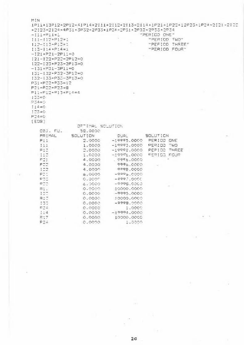
MIN1P11+13P12+2P12+41P +2I23+2I24*4P31+3P3 - I l i + o i l = i I i 1 - 112 + P 1 2 - 1112-113-*-P13=l113-1lfl+P14 = l- 12 1 + P 2 1-2P11=0I 2 1 - I22 + P22-2P12=0I22-I23+P23-2P13=0- 13 1 + P 3 1-3P11=0I31-I32+P32-3P12=0I 3 2 - I33+P33-3P13=0P31+P32+D 33=12P21+P22+P23=8Pli+Pi2-‘-D 13 + P l ‘1 = 4133=0?34=0ri4=oI 23=0P24 =0[ EOB ]

14 + 2111+2112 + 2113 + 21 1 4 + 1P2I+ 1P22+12F2! 2+2P33+lP3«+2P31+2P32+2D 33+2P34

"PER I CD ONE""PERIOD TWO"" P £ P T Q 0 J U R E E "

"PERIOD POUR"

O B J . FU. PR I MAL PI 1 1 1 1

P 2 1 F22 I 22p z :C- — -

7Ri - I 27 R17 133 0 3 -114r \ i, /c : :

58SOLUT

I MAL 50LUT . 0000 I O N

. 0000

. 0000

. 0000 • 0000 — .0000 . 0000 . 0000 . 0000 . 00 or . 0000 . 0000 . 0000 . 0000 . 0000 . 0000 . 0000 . 0000 .0000

I ON

d u a l■ 1 9 9 9 5 , . 190931

• 1 9 9 9 3 .. 1 99C L 1 . 9 9 9 6 ,

9 9 9 6 . 9 ° 9 8 .

- ? o o s ,- 9 9 9 7 i

- 9 9 9 S .1 0 0 0 0 . -9 9 9 5. J 0 0 0 0 .

- 9 9 9 9 .± <

. 1 9 9 9 .0.10000 ,

00000000000000000 0 0 0000000000 0 0 0

000000000000000000000000000000000000C>

SOLUTIONDERIOD o n e PERIOD TWO PERIOD THREE PERIOD FOUR

2c

+ 1P24+2I22 +212

OPTIMAL SOLUTIONOBJ. FU. 47.0000PRIMAL SOLUTION DUAL SOLUTIONPll 1.0000 -19995.0000 PERIOD ONEP12 1.0000 -19994.0000 PERIOD TWOP13 2.0000 -19995.0000 PERIOD THREE113 1.0000 -19993.0000 FERIOD FOURP21 4.0000 -9999.0000121 3.0000 -9997.0000122 2.0000 -9995.0000P31 1.0000 -19992.0000P32 1.0000 -19994.0000P33 2.0000 -19996.0000133 1.0000 -19994.0000P41 1.0000 -9996.0000P42 1.0000 -9997.0000P43 2.0000 -9998.0000R15 0.0000 10000.0000R16 0.0000 10000.0000R17 0.0000 10000.0000R18 0.0000 10000.0000

MIN4P11+3P12+2P12+1P14+2I11+2112+2113+1P21+13P22+12P23+11P24-2I21- +3P32+2F33+1P34+2I31+2132+2133+2I34+4P41+3P42+2P43+1P44+2I41+21 -I11+P11=1 "PERIOD ONE"111-I12+P12=1 "PERIOD TWO"112-113+P13=1 "PERIOD THREE"113+?14=.l "PER I OF FOUR"-I21+P21-P11=0I21-I22+P22-P12=0I22+P23-P13=0-I31+P31=l131-I32+P32=l132-I33+P33=l I33+P34=l -I41+P41-P31=0141-142+P42-P32=0I42+P43-P33=0Pll+P12+P13+P14=4P21+P22+P23=4P41+P42+P43=4P31+P32+P33+P34=4[EOB]

2d

.u 1 )

IO i-i

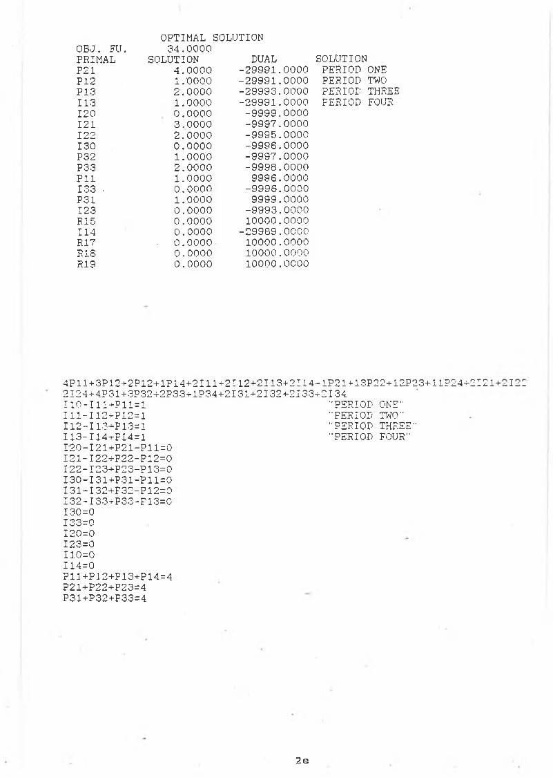
OPTIMAL SOLUTIONO B J . F U . 3 4 . 0 0 0 0

P R I M A L S O L U T I O N D U A L S O L U T I O N

P 2 1 4 . 0 0 0 0 - 2 9 9 9 1 . 0 0 0 0 P E R I O D O N E

P 1 2 1 . 0 0 0 0 - 2 9 9 9 1 . 0 0 0 0 P E R I O D T W O

P 1 3 2 . 0 0 0 0 - 2 9 9 9 3 . 0 0 0 0 P E R I O D T H R E E

1 1 3 1 . 0 0 0 0 - 2 9 9 9 1 . 0 0 0 0 P E R I O D F O U R

1 2 0 0 . 0 0 0 0 - 9 9 9 9 . 0 0 0 0

1 2 1 3 . 0 0 0 0 - 9 9 9 7 . 0 0 0 0

1 2 2 2 . 0 0 0 0 - 9 9 9 5 . 0 0 0 0

1 3 0 0 . 0 0 0 0 - 9 9 9 6 . 0 0 0 0

P 3 2 1 . 0 0 0 0 - 9 9 9 7 . 0 0 0 0

P 3 3 2 . 0 0 0 0 - 9 9 9 8 . 0 0 0 0

P l l 1 . 0 0 0 0 9 9 9 6 . 0 0 0 0

1 3 3 . 0 . 0 0 0 0 - 9 9 9 6 . 0 0 0 0

P 3 1 1 . 0 0 0 0 9 9 9 9 . 0 0 0 0

1 2 3 0 . 0 0 0 0 - 9 9 9 3 . 0 0 0 0

R 1 5 0 . 0 0 0 0 1 0 0 0 0 . 0 0 0 0

1 1 4 0 . 0 0 0 0 - 2 9 9 8 9 . 0 0 0 0

R 1 7 - 0 . 0 0 0 0 - 1 0 0 0 0 . 0 0 0 0

R 1 8 0 . 0 0 0 0 1 0 0 0 0 . 0 0 0 0

R 1 9 0 . 0 0 0 0 1 0 0 0 0 . 0 0 0 0

4 P 1 1 + 3 P 1 2 + 2 P 1 2 + 1 P 1 4 + 2 I I 1 + 2 1 1 2 + 2 1 1 3 + 2 1 1 4 + 1 P 2 1 + 1 3 P 2 2 + 1 2 P 2 3 + 1 I P

2 I 2 4 + 4 P 3 1 + 3 P 3 2 + 2 P 3 3 + 1 P 3 4 + 2 I 3 1 + 2 I 3 2 + 2 I 3 3 + 2 I 3 4

1 1 0 - 1 1 1 + P 1 1 = 1 " P E R I O D O N E "

1 1 1 - I 1 2 + P 1 2 = l " P E R I O D T W O "

1 1 2 - 1 1 3 - ^ 1 3 = 1 " P E R I O D T H R E E "

1 1 3 - I 1 4 + P 1 4 = l " P E R I O D F O U R "

1 2 0 - I 2 1 + P 2 1 - P 1 1 = 0

1 2 1 - I 2 2 + P 2 2 - P 1 2 = 0

1 2 2 - I 2 3 + P 2 3 - P 1 3 = 0

1 3 0 - I 3 1 + P 3 1 - P 1 1 = 0

1 3 1 - I 3 2 + P 3 2 - P 1 2 = 0

1 3 2 - I 3 3 + P 3 3 - F 1 3 = 0

1 3 0 = 0

1 3 3 = 0

120=01 2 3 = 0

110=01 1 4 = 0

P l l + P 1 2 + P 1 3 + P 1 4 = 4

P 2 1 + P 2 2 + P 2 3 = 4

P 3 1 + P 3 2 + P 3 3 = 4

9 4-^° 12 1 I

2 e

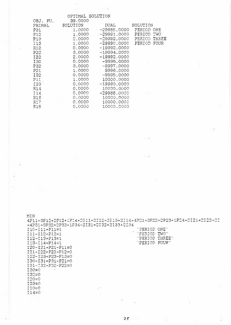
OPTIMAL SOLUTIONOBJ. FU. 39.0000PRIMAL SOLUTION DUAL SOLUTIONP31 1.0000 -29988.0000 PERIOD ONEP12 1.0000 -29991.0000 PERIOD TWOP13 2.0000 -29992.0000 PERIOD THREE113 1.0000 -29990.0000 PERIOD FOURR12 0.0000 -19992.0000P22 3.0000 -19994.0000122 2.0000 -19992.0000130 0.0000 -9996.0000P32 3.0000 -9997.0000P21 1.0000 9996.0000132 0.0000 -9995.0000Pll , 1.0000 10000.0000123 0.0000 -19990.0000R14 0.0000 10000.0000114 0.0000 -29988.0000R1S 0.0000 10000.0000R17 0.0000 10000.0000R1S 0.0000 10000.0000

MIN4P11+3P12+2P12+1PI4+2 II 1+2112+2113+2114+4P21+3P22+2P23+1P24+2121+2122-t-2I +4P31+3P32+2P33+1P34+2131+2132+2133+2134110-I11+P11=1111-I12+P12=l112-I13+P13=1113-114+P14=1120-I21+P21-P11=0121-I22+P22-P12=0122-I23+P23-P13-0130-I31+P31-P21-0131-I32+P32-P22=0 130=0132=0120=0123=0110=0

"PERIOD■■ piT'jTnri"PERIOD"PERIOD

ONE"TWO"THREE"FOUR"

2 f

A P P E N D I X 3 A S C I C O N I C M o d e l I n p u t

SUFFICES A MAXA 1 I MAXI 5

CC MAX NUMBER OF FACILITIES CT MAXT 25

CC MAX NO DT TIME PERIODS - CEXTERNAL VALUES PCOSTSfI,T)

CC PRODUCTION COSTS DEFINED FOR EACH FACILITY IN EVERY TIME PERIOD CHCOSTS(I,T )

CC H0LDIN6 COSTS DEFINED FDR EACH FACILITY IN EACH TIME PERIOD CDEMiT)

CC DEMAND AT FINAL FACILITY IN EVERY TIME PERIOD CVARIABLES IN(IJ) 'ttIT'

nV.

C INVENTORY CARRIED FROM PERIOD TO NEXT PERIOD CPR(I,T) ■HIT'

CC INVENTORY PRODUCED IN A GIVEN PERIOD AT A GIVEN FACILITY CPROBLEM MINIMISE tCOST 'tit*'SUM(I.T) PQ1IPR(I, T)

+SUM(I,T) HQ1tIN(I,T )SUBJECT TO IMATBB ‘i m i l T *IN(I,T1)-IN(I,T)+PR(I,T).EQ.D01

FOR ALL T FOR 1=1 FOR T1=T-1 CC MATERIAL BALANCE CONSTRAINT AT FIRST FACILITY CtHATB 'ttttlT'IN(I,T1)-IN(I,T)+PR(I,T)-PR(U,T) .EQ.COl

FOR 1=2 FOR T1=T-1 FOR 11=1-1

»3Aa

FOR ALL T CC MATERIAL BALANCE AT SECOND FACILITY«m at ,m i rIN(I,T1)-IN(I,T)+PR(I,T)-PR(I1,T).EQ.COl

FOR 1=3 FOR T1=T-1 FOR 11=1-2 FOR ALL T CC MATERIAL BALANCE AT THIRD FACILITY CICAP 'till'

SUM(T) PR(I,T).EQ.QOl FOR 1=1 CC ACCUMULATED PRODUCTION AT THE FIRST FACILITYCCELEMENTS

P01=PC0STS(I,T)H01=HC0STS(I,T)D01=DEM(T)C01=0.0001=24.0

EHDATA

3 Ab

APPENDIX 3B

Matrix Generation Data File

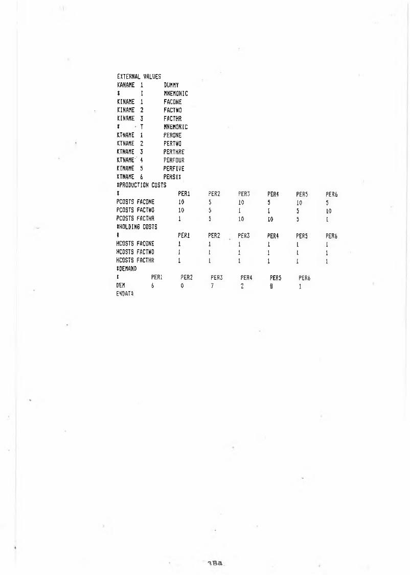
EXTERNAL VALUESKANAHE 1 DUMMYt I MNEMONICKINANE 1 FACONEKINAME 2 FACTHOKINAME 3 FACTHR* T MNEMONICKINANE 1 PERONEKTNAME 2 PERTHOKTNAME 3 PERTHREKTNAME' 4 PERFOURKTNAME 5 PERFIVEKTNANE 6 PERSI X»PRODUCTION COSTS» PERIPCOSTS FACONE 10PCOSTS FACTHO 10PCOSTS FACTHR 1IH0LDIN6 COSTS1 PERIHCOSTS FACONE 1HCOSTS FACTHO 1HCOSTS FACTHR 1»DEMANDt PERI PER2DEN 6 0ENDATA

PER2 PER3 PER4 PER5 PERÌ5 10 5 10 55 1 1 5 105 10 10 5 I

PER2 PER3 PER 4 PER5 PER61 1 1 1 I1 1 1 1 1I 1 1 1 1

PER3 PERÌ PER5 PER67 nL 8 1

APPENDIX 3C

Matrix File

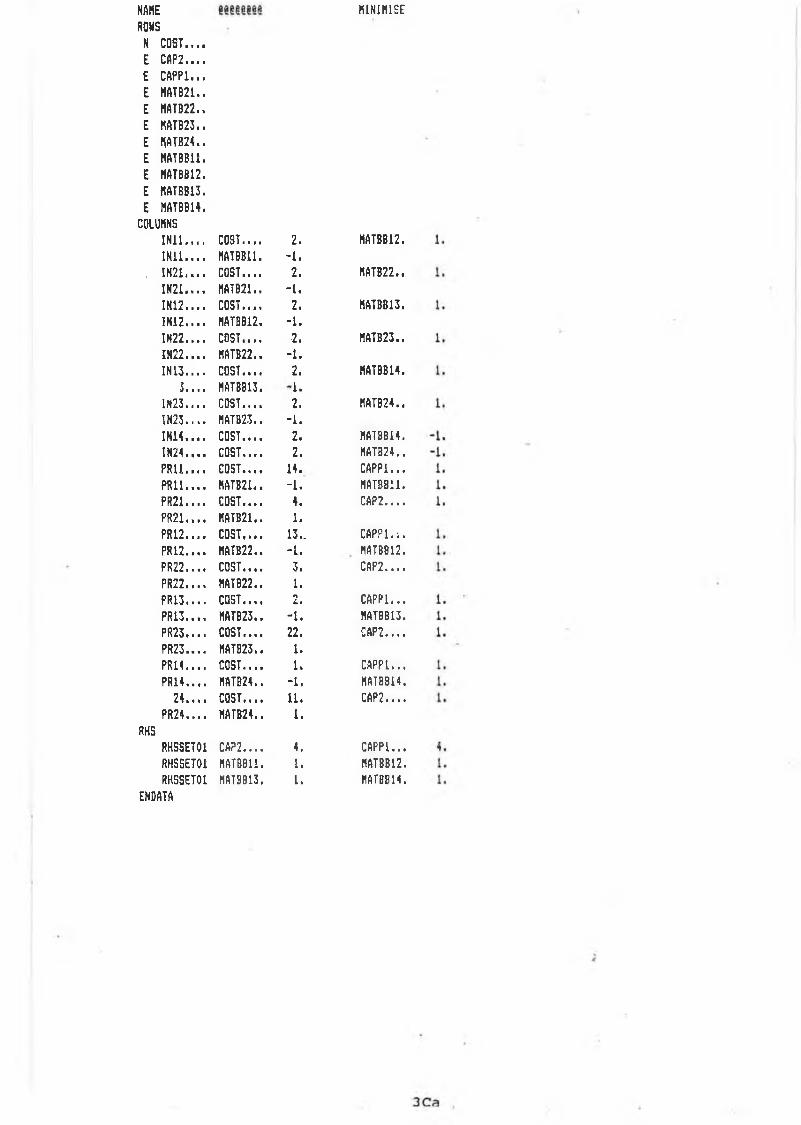
NAME MINIMISEROWSN COST.,.. E CAP2..,. E CAPP1... E MATB21.. E MATB22.. E MATB23.. E HATB24.. E HflTBBll. E MATBB12. E HATBB13. E MATBB14.

COLUMNSINI1.... COST.... 2. MATBB12IN11.... MATBB11. -I.

, IN21.... COST.... 2. MATB22.IN2L... MATB21.. -1,IN12.... COST.... 2. MATBB13IN12.... MATBB12. -1.IN22.,., COST..,. 2. MATB23.IN22.... MATB22.. -i.IN13.... COST.... 2. MATBB14

J.... HATBB13.LN23.... COST.... 2. HATB24.IN23.... HATB23.. -1.IN14.... COST.... 2. MATBB14IN24.... COST.... 2. MATB24.PRU.... COST.... 14. CAPP1..PR11.... HATB21,. -1. MATBB11PR21.... COST.... 4. CAP2...PR21.... HATB21.. 1.PR12.... COST.... 13. CAPPl.iPR12.... MATB22 . -L, MATBB12PR22.... COST.... 3. CAP2...PR22.... MATB22.. 1.PR13.... COST..,. CAPP1..PR13.... MATB23.. -1. MATBB13PR23__ COST.... 22. CAP2...PR23__ MATB23.. 1.P R U __ COST.... 1. CAPP1..PR14.... HATB24.. -1. MATBB14

24.... COST.... 11. CAP2...PR24.... MATB24.. 1.

RHSRHSSET01 CAP2.... 4. CAPP1..RHSSETOi MATBB11. 1. HATBB12RHSSET01 MATBB13. 1. MATB814

ENDATA

APPENDIX 3D

SCICONIC Results

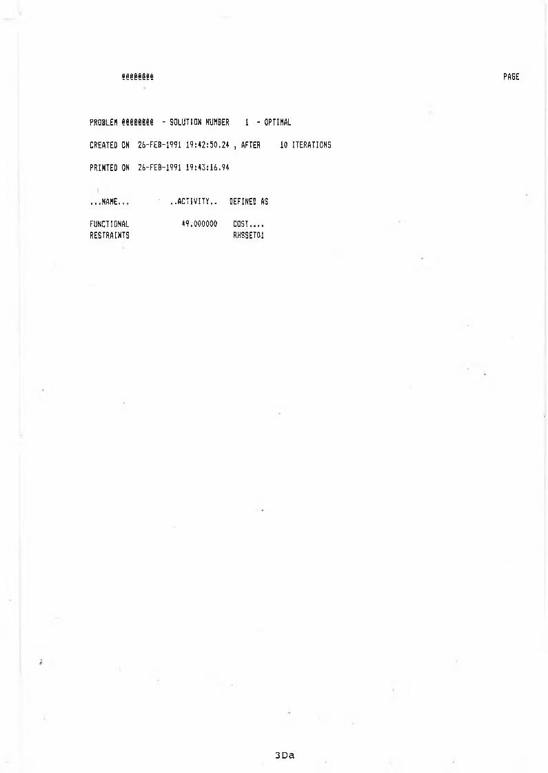
eee§§eee PAGE

PROBLEM e§§8@g«§ - SOLUTION HUMBER 1 - OPTIMAL

CREATED ON 26-FEB-1991 19:42:50.24 , AFTER 10 ITERATIONS

PRINTED ON 2 6 - F E B - i m 19:43:16.94

...NAME,.. • ..ACTIVITY.. DEFINED AS

FUNCTIONAL 49.000000 COST....RESTRAINTS RHSSET01

3D a

12345678

• 91011

tER12131415161718192021222324252627

( M e e e i i

..ROM... AT ....ACTIVITY.... .SLACK ACTIVITY. ..LOUER BOUND... ..UPPER BOUND...COST.■•i BS 49.000000 -49.000000 HONE NONECAP2.I.. EQ 4.000000 a 4.000000 4.000000CAPP1... EQ 4.000000 ■ 4.000000 4.000000HATE21 . EO » • ■HATB22.. EQ • • •

HATB23. - EQ t • , u

MATB24 . EQ • • ■

HATBB11. EQ 1 . 0 0 0 0 0 0 • 1 . 0 0 0 0 0 0 1 . 0 0 0 0 0 0

HATBB12. EQ 1 . 0 0 0 0 0 0 • 1 . 0 0 0 0 0 0 1 . 0 0 0 0 0 0

RATBB13. EQ 1 . 0 0 0 0 0 0 • 1 . 0 0 0 0 0 0 1 . 0 0 0 0 0 0

HATBB14, EQ 1 . 0 0 0 0 0 0 • 1.000000 1 . 0 0 0 0 0 0

.COLUMN. AT ....ACTIVITY.... ...INPUT COST... ..LOWER BOUND... ..UPPER BOUND...IM1.... LL ■ 2.000000 NONEIN21.... LL . 2.000000 NONEIN12.... LL . 2.000000 NONEIN22.... BS 2.000000 2.000000 NONEIN13.... LL . 2.000000 NONEIN23.... BS i.000000 2.000000 NONEIN14.... LL • 2.000000 NONEIN24.... LL 1 2.000000 NONEPR11__ BS 1.000000 14.000000 NONEPR21__ BS 1.000000 4.000000 NONEPR12__ BS 1.000000 13.000000 NONEPR22.... BS 3.000000 3.000000 NONEPR13.... BS 1.000000 2.000000 NONEPR23.... LL ■ 22.000000 NONEPR14.... BS 1.000000 1.000000 NONEPR24.... LL 1 11.000000 NONE

t nV\

APPENDIX 4A

SIMAN Model File

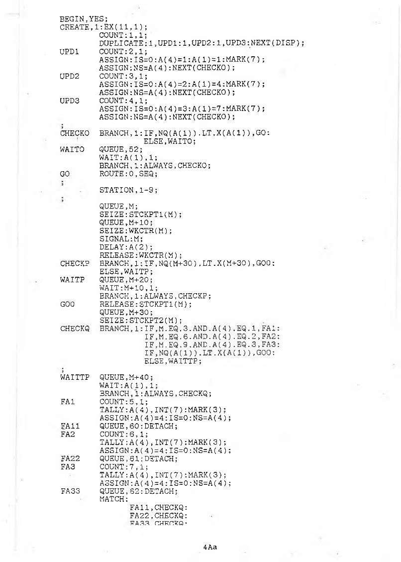
BEGIN,YES;CREATE, 1:E X (11,1);

COUNT:1,1;DUPLICATE:1,UPD1:1,UPD2:1,UPD3:NEXT(DISP);

UPD1 COUNT:2,1;ASSIGN:IS=0:A(4 )=1:A(1)=1:MARK(7);ASSIGN:NS=A(4):NEXT(CHECKO);

UPD2 COUNT:3,1;ASSIGN;IS=0:A(4 )=2:A(1)=4:MARK(7);ASSIGN:NS=A(4):NEXT(CHECKO);

UPD3 COUNT:4,1;ASSIGN:IS=0:A(4 )=3:A(1)=7:MARK(7);ASSIGN:NS=A(4):NEXT(CHECKO);

CHECKO BRANCH,1:IF,NQ(A(1)).LT.X(A(1)),GO:ELSE,WAITO;

WAITO QUEUE,52;WAIT:A (1),1;BRANCH,1:ALWAYS,CHECKO;

GO ROUTE:0,SEQ;

STATION,1-9;

QUEUE,M;SEIZE:STCKPTl(M);QUEUE,M+10;SEIZE:WKCTR(M);SIGNAL:M ;DELAY:A (2);RELEASE:WKCTR(M);

CHECKP BRANCH,l:IF,NQ(M+30).LT.X(M+30),GOO: ELSE,WAITP;

WAITP QUEUE,M+20;WAIT:M+10,1;BRANCH,1:ALWAYS,CHECKP;

GOO RELEASE:STCKPTl(M);QUEUE,M+30;SEIZE:STCKPT2(M);

CHECKQ BRANCH,1:IF,M.EQ.3.AND.A (4).EQ.1,FA1IF,M.EQ.6.AND.A(4).EQ.2,FA2 IF,M .EQ.9.AND.A (4).EQ.3,FA3 IF,NQ(A (1))•LT.X (A (1)),GOO: ELSE,WAITTP;

WAITTP QUEUE,M+40;W AIT “ A (1) 1 *BRANCH,1:ALWAYS,CHECKQ;

FA1 COUNT:5,1;TALLY:A (4),INT(7):MARK(3); ASSIGN:A(4)=4:IS=0:NS=A(4);

FA11 QUEUE,60:DETACH;FA2 COUNT:6,1;

TALLY:A (4),INT(7):MARK(3); ASSIGN:A(4 )=4:IS=0:NS=A(4);

FA22 QUEUE, 61 .-DETACH;FA3 COUNT:7,1;

TALLY:A(4),INT(7):MARK(3); ASSIGN:A(4)=4:IS=0:NS=A(4);

FA33 QUEUE,62:DETACH;MATCH:

FA11,CHECKQ:FA22,CHECKQ:

r.H irr.htq■

4A a

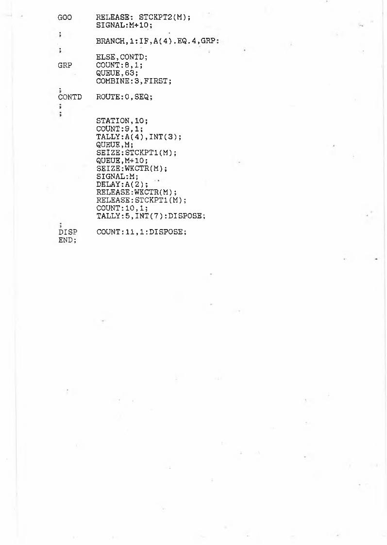
GOO RELEASE: STCKPT2(M);SIGNAL:M+10;

« m

BRANCH,1:IF,A(4).EQ.4,GRP*

ELSE,CONTD;GRP COUNT:8,1;

QUEUE,63;COMBINE:3,FIRST;

aCONTD ROUTE:0,SEQ;

STATION,10;COUNT:9,1;TALLY:A (4),INT(3); QUEUE,M;SEIZE:STCKPT1(M);QUEUE,M+10;SEIZE:WKCTR(M); SIGNAL:M;DELAY:A(2);RELEASE:WKCTR(M); RELEASE:STCKPT1(M); COUNT:10,1;TALLY:5,INT(7):DISPOSE;

DISP COUNT:11,1:DISPOSE;END;

APPENDIX 4B

SIMAN Experimental File

BEGIN, ,Y E S ; .PROJECT,KANBAN,TG,20/6/90;

DISCRETE,250,7,65,10;A T T R IB UT ES:7;

RESOURCES:1-10,WKCTR,1,:11-20,STCKPT1,1:21-30,STCKPT2,1;

INITIALIZE,X(1)=1,X(2)=1,X(3)=1,X(4)=1,X(5)=1,X(6)=1,X(7)=: X (9)=1,X (10)=1,X ( 31) =1,X (32)=1,X ( 3 3 ) = 1 , X (34)=1,X (35)=1,X (36)=1 X (38)=1,X(39)=1,X(40)=1;

SEQUENCES :-l , 2 ,3,4 ,

1,2,R N (1,1)& 2,3,R N (2,1)& 3,10,R N (3,1): 4,5,R N (4,1)& 5,6,R N ( 5 ,1) & 6,10,R N (6,1): 7,8, RN ( 7 , 1) & 8,9, RN ( 8 , 1 ) & 9,10,R N (9,1): 10,,R N (10,1);

PARAMETERS:1, 2 ,3,4,5,6 , 7 ,8 , 9 ,

15, . 15, . 15, . 15, . 15, . 15, . 15, . 15, . 15, .

10,17,1: 1 1 ,8 ;

D S T A T : 1,N O (1),INBUFQ1:2 , N Q ( 2 ) ,INBUFQ2:3,N Q (3) , I N B U F 0 3 :4 ,NQ(4) , INBUFQ4:5,NQ(5 ) , INBUFD5:6, N Q (6),INBUFQ6:7 , N Q ( 7 ) ,INBUFQ7:8,N Q (8) , INBUFQ8, "KAN.8" :9,N Q (9),INBUFQ9,"KAN.9":10,NQ(10) , INBUFQ10,"KAN.10"

,0 U TB UF Q1,"KAN.31" ,0UTBUFQ2,"KAN.32", 0UTB UF Q3,"KAN.3 3 ”,0 U TB UF Q4:,D U TB UF Q5:,0 U TB UF Q6:,Q U TB UF Q7:,0U T B U F Q 8 :,0U T B U F Q 9 :,0U TB U F Q 1 0 ,"KAN.40" :

31 ,N Q (31)32,N Q (32)33 ,N Q (33)34,N Q (34)35 ,N Q (35)36 ,N Q (36)37 ,N Q (37)38,N Q (3fe)39,N Q (39)4 0 ,NQ(40)4 1 ,NR(1 ) ,UTIL1:42 ,N R (2),U T I L 2 :43,N R (3),U T I L 3 :44,N R (4),U T I L 4 :45,N R (5),U T I L 5 :46,N R (6),U T I L 6 :

, X (37)

1 , X ( 8 )

47 ,NR(7),UT IL7:48,N R (8),UT L1L 8 :4 9 , N R ( 9 ) , U T I L 9 : .50,N R (10),UT IL10;

COUNTERS:1,SYS CREATED:2,NO TYP 1:3,NO TYP 2:4,NO TYP 3:5,NO TYP 1 ST.3:6,NO TYP 2 S T ,6:7,NO TYP 3 ST.9:8,NO ENT COMB Q:9,NO ST 10:10,NO DISP S T 1 0 :11,NO DUP DISP;

;REPLI C A T E ,5,0,530,Y E S ,Y E S ,50 ; REPLICATE,1,0,480;

TALLIES:1,LEAD-TIME.PT.1:2,LEAD.TIME.PT.2:3,LEAD.TIME.PT.3:4,WAIT TIME FA:5,OVERALL FLOWTIME;

END;

A O K

APPEND EX 5

Nomenclature

SUFFICES

1. k: products\end-items 1...M

2. i: facilities 1 ...N

3 - , t: time periods 1 ...T

4. d: no. o f machine resources at a facility

5. Ci): immediate successor (parent) o f facility i

6. Li: lead-time stage i

SETS

1. P(i) set o f immediate predecessor stages

2. S(i) . set o f all successor stages

5a

VARIABLES

1. P .(P*> : production of product K, facility i, period t.

2. h (U : inventory held product k, facility i, period t.

3. V inventory in storage facility i, period t.

4. In' inventory in shortage, at facility i, period t.

5. Q» lot size to be determined at facility i.

6. Ki fixed cost o f ordering production at facility i.

7. Pi production or assembly rate at facility i.

8. p rate at which demand is being met (D/Pi)

9. no. o f times product k must be produced in first t

periods to ensure positive inventory level at the end of

10. X*

11. Ya

12. W„

13.

14.

15.

16.

Uu

S*

V*

O*

t periods.

no. o f facilities scheduled to produce product k during

period t.

integer variable value 0,1.

summed requirements facility i, less initial inventory

due to independent demand less firm scheduled receipts

plus and dependent demand from any parent items or

for item i in period t.

net requirements facility i period t.

ab so lu te ca p a c i ty c o n s tr a in t on further

purchasing\production.

undertime requirements at resource d, period t

overtime requirements at resource d, period t.

5 b

CONSTANTS

1. Cu (Q J: production costs product k, facility i, period, t.

2. Hy, (H**): holding costs product k, facility i, period t.

3. D u (D^): demand costs product k, facility i, period t.

4. Hü+ : inventory storage costs at end o f period t.

5. Hu_ : inventory shortage costs at end o f period t.

6. K, : fixed cost o f ordering (production) at stage

7. /il; : holding cost per unit time charged against echelon stock

at stage i.

8. T : planning horizon length

9. : production charge per product k, made up of fixed

production rate per product (P^ and a unit inventory

charge (0J ¥ = Vz Pk

10. Pit : production capacity facility i, period t.

11. IH : inventory storage capacity facility i, period t.

12. Mti : yield factor at facility i, product k.

13. Su : set-up cost facility i, period t.

14. Eu : unit requirement o f type d, resource constraint in

production at facility i.

15. M : very large no.

16. 4 , : inventory at facility i, period o.

5 c

17. bu : per unit production time, facility i, resource d.

18. Su : set-up time, facility i, resource d.

19. 0 * overtime required, resource d > facility t.

20. U* : undertime required, resource d, facility t.

21. 0>* : overtime costs required, resource d, facility t.

22. Cu£ . undertime costs required, resource d, facility*.

23. Cap* : total capacity available, resource d, facility t.

APPENDIX 6

Tables of Results: (6.18a, 6.18b, 6.19a, 6.19b)

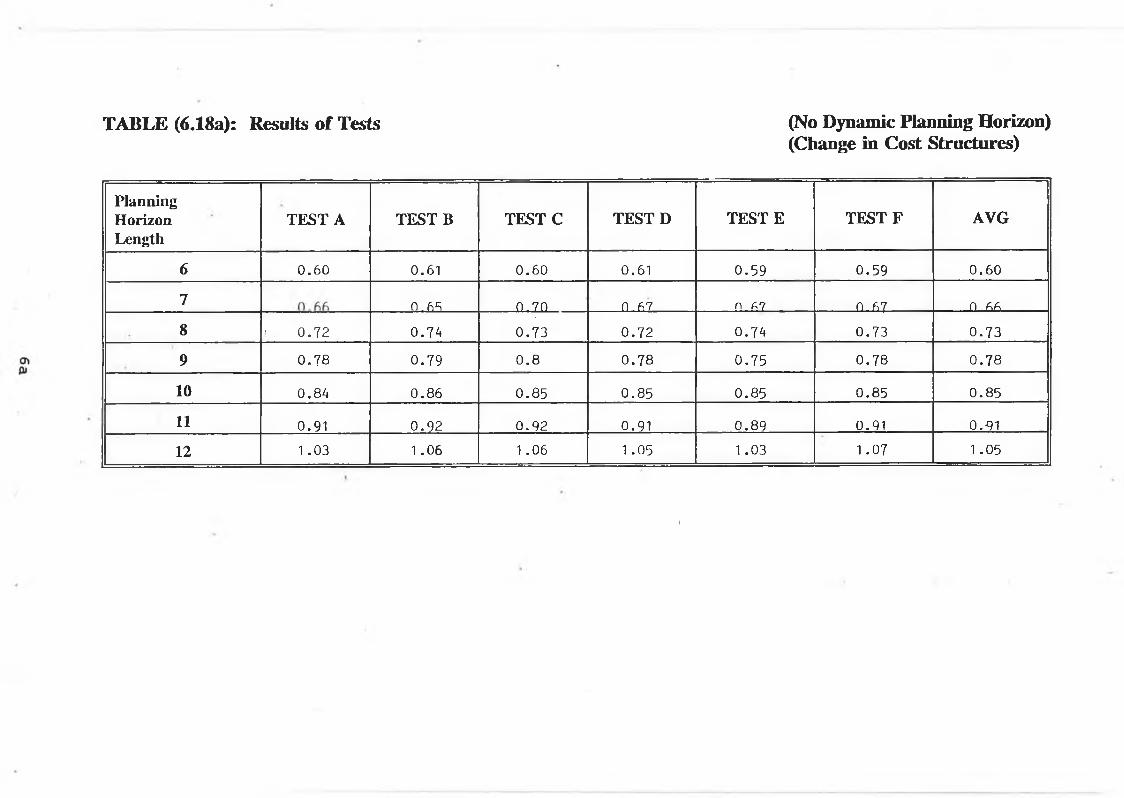
TABLE (6.18a): Results o f Tests (No Dynamic Planning Horizon)(Change in Cost Structures)

PlanningHorizonLength

TESTA TEST B TEST C TEST D TESTE TEST F AVG

6 0 .60 0.61 0 .60 0.61 0.59 0.59 0 .60

7 n .6^ 0 .70 0.67 n A 7 n ^7 n .fifi

8 1 0 .72 0 .74 0 .73 0 .72 0.74 0 .73 0 .73

9 0 .78 0 .79 0 .8 0 .78 0 .75 0 .78 0 .78

10 0.84 0 .86 0 .85 0 .85 0.85 0.85 0 .85

11 0.91 0 .92 0 .92 0.91 0 .89 0.91 0.91

12 1 .03 1 .06 1 .06 1 .05 1.03 1 .07 1 .05

I

TABLE (6.19a): Results o f Tests (With Dynamic Planning Horizon)(Change in Cost Structures)

PlanningHorizonLength

TEST A TEST B TEST C TEST D TEST E TEST F AVG

6 0.36 0 .36 0 .40 0.34 0.34 0 .36 0 .36

78 0.48 0.49 0.47 0 .48 0.46 0.50 0 .48

910 0 .62 0.63 0.61 0 ,62 0 .63 0 . 6 ?

1112 0.85 0 .79 0 .79 0.81 0.81 0.81 0.81

;jy

TABLE (6.18b): Results o f Tests (No Dynamic Planning Horizon)(Change in Cost Structures)

PlanningHorizonLength

T E S T A T E S T B T E S T C T E S T D T E S T E T E S T F A V G

6 0 . 4 4 0 . 46 0 . 4 2 0 . 4 3 0 . 4 2 0 . 4 4 0 . 4 4

7 0 . 4 6 0 . 4 8 0 . 4 4 0 . 4 3 0 . 4 7 0 . 4 6 0 . 4 6

8 0 . 4 8 0 . 4 4 0 . 5 0 0 . 4 5 0 . 50 0 . 4 7 0 . 4 7

9 0 . 5 0 0 . 4 8 0 . 53 0 . 4 9 0 . 5 1 0 . 4 9 0 . 50

10 0 . 5 2 0 . 4 9 0 . 5 3 0 . 5 4 0 . 5 0 . 5 1 0 . 5 2

11 0 . 5 4 0 . 52 0 . 4 9 0 / 5 5 0 . 5 7 0 . 5 5 0 . 5 4

12 0 . 56, 0 . 52 0 . 58 0 . 5 9 0 . 5 2 0 . 5 1 0 . 5 5

i

es

TABLE (6.19b): Results o f Tests (With Dynamic Planning Horizon)(Change in Cost Structures)

PlanningHorizonLength

T E ST A TEST B TEST C TEST D TEST E TEST F AVG

6 0 .38 0 .40 0 .36 0.41 0 .36 0.35 0 .38

7

8 0.42 0.44 0 .39 0 .43 0 .42 0.41 0 .42

9

10 0 .49 0 .50 0 .50 0 .4 8 0.47 0 .52 0 .49

11

12 0 .50 0.51 0 .52 0 .48 0.49 0 .50 0 .50