Medipix calibration experiments and theory MSarajlic -...

Medipix calibration experiments and theory

Milija Sarajlic

DESY from 01. 09. to 30. 11. 2010

of 30

Milija Sarajlic, Medipix sensor testing at DESY, 01.09.-30.11.2010.

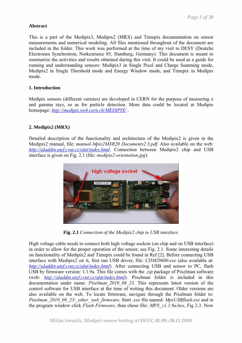
Abstract This is a part of the Medipix3, Medipix2 (MRX) and Timepix documentation on sensor measurements and numerical modeling. All files mentioned throughout of the document are included in the folder. This work was performed at the time of my visit to DESY (Deutche Electronen Synchrotron, Notkestrasse 85, Hamburg, Germany). This document is meant to summarize the activities and results obtained during this visit. It could be used as a guide for running and understanding sensors: Medipix3 in Single Pixel and Charge Summing mode, Medipix2 in Single Threshold mode and Energy Window mode, and Timepix in Medipix mode. 1. Introduction Medipix sensors (different varietes) are developed in CERN for the purpose of measuring x and gamma rays, so as for particle detection. More data could be located at Medipix homepage: http://medipix.web.cern.ch/MEDIPIX/ . 2. Medipix2 (MRX) Detailed description of the functionality and architecture of the Medipix2 is given in the Medipix2 manual, file: manual-Mpix2MXR20 Documentv2.3.pdf. Also available on the web: http://aladdin.utef.cvut.cz/ofat/index.html. Connection between Medipix2 chip and USB interface is given on Fig. 2.1 (file: medipix2-orientation.jpg).

Fig. 2.1 Connection of the Medipix2 chip to USB interface.

High voltage cable needs to connect both high voltage sockets (on chip and on USB interface) in order to allow for the proper operation of the sensor, see Fig. 2.1. Some interesting details on functionality of Medipix2 and Timepix could be found in Ref [2]. Before connecting USB interface with Medipix2 on it, first run USB driver, file: CDM20600.exe (also available at: http://aladdin.utef.cvut.cz/ofat/index.html). After connecting USB and sensor to PC, flash USB by firmware version: 1.1.9a. This file comes with the .zip package of Pixelman software (web: http://aladdin.utef.cvut.cz/ofat/index.html). Pixelman folder is included in this documentation under name: Pixelman_2010_08_23. This represents latest version of the control software for USB interface at the time of writing this document. Older versions are also available on the web. To locate firmware, navigate through the Pixelman folder to: Pixelman_2010_08_23\_other_\usb_firmware. Start .exe file named: MpxUSBflash.exe and in the program window click Flash Firmware, than chose file: MPX_v1.1.9a.hex, Fig 2.3. Now

of 30


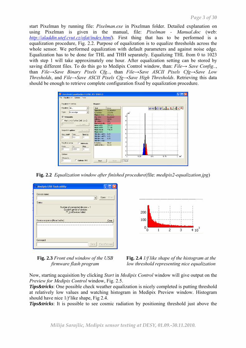
start Pixelman by running file: Pixelman.exe in Pixelman folder. Detailed explanation on using Pixelman is given in the manual, file: Pixelman - Manual.doc (web: http://aladdin.utef.cvut.cz/ofat/index.html). First thing that has to be performed is a equalization procedure, Fig. 2.2. Purpose of equalization is to equalize thresholds across the whole sensor. We performed equalization with default parameters and against noise edge. Equalization has to be done for THL and THH separately. Equalizing THL from 0 to 1023 with step 1 will take approximately one hour. After equalization setting can be stored by saving different files. To do this go to Medipix Control window, than: File→ Save Config.., than File→Save Binary Pixels Cfg.., than File→Save ASCII Pixels Cfg→Save Low Thresholds, and File→Save ASCII Pixels Cfg→Save High Thresholds. Retrieving this data should be enough to retrieve complete configuration fixed by equalization procedure.

Fig. 2.2 Equalization window after finished procedure(file: medipix2-equalization.jpg)

Fig. 2.3 Front end window of the USB

firmware flash program

Fig. 2.4 1/f like shape of the histogram at the low threshold representing nice equalization

Now, starting acquisition by clicking Start in Medipix Control window will give output on the Preview for Medipix Control window, Fig. 2.5. Tips&tricks: One possible check weather equalization is nicely completed is putting threshold at relatively low values and watching histogram in Medipix Preview window. Histogram should have nice 1/f like shape, Fig 2.4. Tips&tricks: It is possible to see cosmic radiation by positioning threshold just above the

of 30


Fig. 2.5 Cosmic radiation as recorded by Medipix2 sensor.

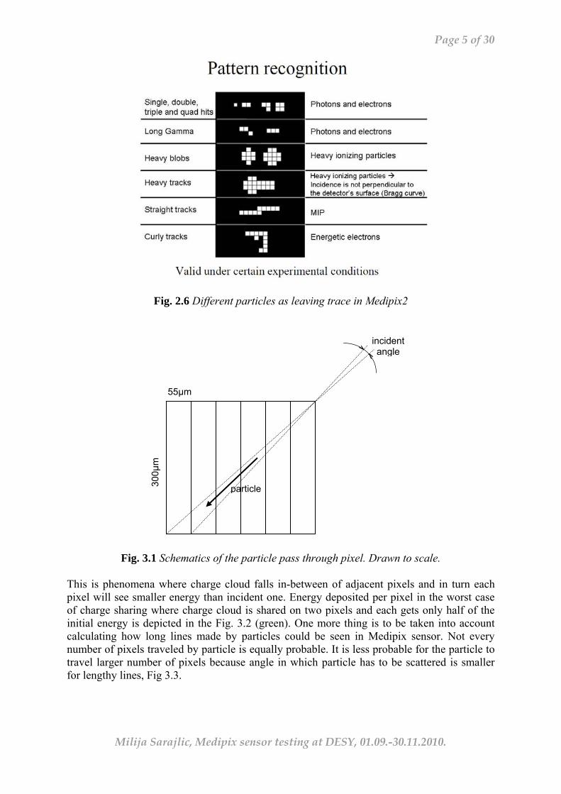
noise level and taking integrated acquisition, Fig 2.5. Seeing cosmic is actually a good test weather sensor is functioning properly. If you are not able to see cosmic, than there must be something wrong. Tips&tricks: Some of the very noisy pixels have to be masked in order to make nice functionality of the sensor. Position threshold close to the noise level and mask all pixels that count more than one. There is a trade off between number of the pixels masked and visibility of the screen. More noisy pixels masked will give possibility to operate sensor on the lower threshold but it will in turn reduce active area of the sensor. Tips&tricks: There is a nice presentation about different types of particles that can be recognized by medipix sensor, Ref [3], Fig. 2.6. Tips&tricks: Some pixels can be noisy only in certain range of threshold digital values. Therefore, it is advisable that before beginning real measurements with Medipix sensor of any type, one first scan all threshold digital values of interest, measuring total count, even though those values are high above the noise level. 3. Length of the particle trace Trace length that particle would make in Medipix sensor can be calculated by assuming energy loss that particle suffers is constant along the path. Energy loss for the particle in Si is taken from Ref. [4] (Fig. 27.6 and 27.7 Ref. [4]). Fig. 3.1 gives schematics of the pixel size and particle passage through. Assuming Mean Value energy loss for Si, deposited energy will depend on number of pixels passed, Fig. 3.2 (blue). Energy deposited in material by particle is stochastic process and for operation of sensor more realistic is to take Most Probable Value of energy loss, Ref [4]. This comes as a consequence of the fact that high energy tail of the particle loss is often lost in the background, Ref [4]. Most Probable Value could be only 60% of that for Mean Value. Fig. 3.2 depicts energy loss per pixel assuming Most Probable Value (red). What can also reduce energy collection in the Medipix sensor is charge sharing effect.

of 30


Fig. 2.6 Different particles as leaving trace in Medipix2

Fig. 3.1 Schematics of the particle pass through pixel. Drawn to scale.

This is phenomena where charge cloud falls in-between of adjacent pixels and in turn each pixel will see smaller energy than incident one. Energy deposited per pixel in the worst case of charge sharing where charge cloud is shared on two pixels and each gets only half of the initial energy is depicted in the Fig. 3.2 (green). One more thing is to be taken into account calculating how long lines made by particles could be seen in Medipix sensor. Not every number of pixels traveled by particle is equally probable. It is less probable for the particle to travel larger number of pixels because angle in which particle has to be scattered is smaller for lengthy lines, Fig 3.3.

55μm

300μ

m

incident angle

particle

of 30


Fig. 3.2 Energy generated per pixel in the case of oblique incidence

of the particle [keV] vs. number of the pixels that particle has traveled assuming Mean Energy loss (blue), Most Probable Energy loss (red) and Most Probable Energy loss in addition to worst case charge sharing (green)

Fig. 3.3 Probability that particle will hit more than one pixel vs. number of pixels passed. Probability is scaled to the probability of single pixel hit.

Having in mind all that is said before, for the sensor that has noise level on 8keV, and assuming worst case charge sharing it would be practically very hard to see particle traces longer than 7 pixels in a raw. Some of the frames acquired by Medipix2 are found in the folder: mx2 frames. These frames could be seen by utility Frame Browser available in the Pixelman. Calculations are gathered in Mathematica file: particle energy loss.nb. This effect is also possible to notice if the threshold is scanned from higher values to lower values and cosmic are recorded. In high threshold range only single pixel hits or lines up to two or three pixels will be recorded. As the threshold is shifted towards lower values, suddenly very long particle traces will start to appear. Collection of the cosmic particles scans is stored in folder: ..\mx2 frames\cosmics THL. Scan is performed for THL digital values from 0 to 350. Acquisition per each THL digital value took 10 minutes (600sec).

Number of pixels passed

Ene

rgy

depo

site

d [k

eV/p

ixel

] Mean Energy loss

Most Probable Energy loss

Most Probable Energy loss + worst case charge sharing

Number of pixels passed

Pro

babi

lity

of n

umbe

r of p

ixel

s pa

ssed

sc

aled

to p

roba

bilit

y of

sin

gle

pixe

l hit

of 30


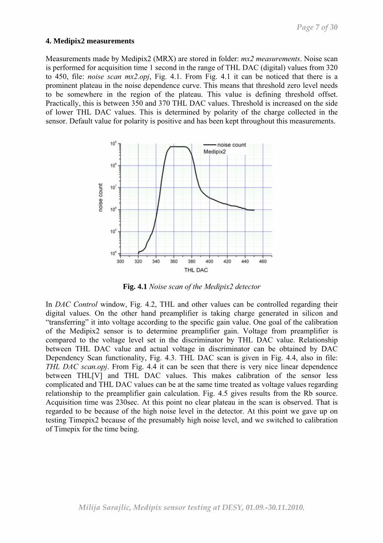
4. Medipix2 measurements Measurements made by Medipix2 (MRX) are stored in folder: mx2 measurements. Noise scan is performed for acquisition time 1 second in the range of THL DAC (digital) values from 320 to 450, file: noise scan mx2.opj, Fig. 4.1. From Fig. 4.1 it can be noticed that there is a prominent plateau in the noise dependence curve. This means that threshold zero level needs to be somewhere in the region of the plateau. This value is defining threshold offset. Practically, this is between 350 and 370 THL DAC values. Threshold is increased on the side of lower THL DAC values. This is determined by polarity of the charge collected in the sensor. Default value for polarity is positive and has been kept throughout this measurements.

Fig. 4.1 Noise scan of the Medipix2 detector

In DAC Control window, Fig. 4.2, THL and other values can be controlled regarding their digital values. On the other hand preamplifier is taking charge generated in silicon and “transferring” it into voltage according to the specific gain value. One goal of the calibration of the Medipix2 sensor is to determine preamplifier gain. Voltage from preamplifier is compared to the voltage level set in the discriminator by THL DAC value. Relationship between THL DAC value and actual voltage in discriminator can be obtained by DAC Dependency Scan functionality, Fig. 4.3. THL DAC scan is given in Fig. 4.4, also in file: THL DAC scan.opj. From Fig. 4.4 it can be seen that there is very nice linear dependence between THL[V] and THL DAC values. This makes calibration of the sensor less complicated and THL DAC values can be at the same time treated as voltage values regarding relationship to the preamplifier gain calculation. Fig. 4.5 gives results from the Rb source. Acquisition time was 230sec. At this point no clear plateau in the scan is observed. That is regarded to be because of the high noise level in the detector. At this point we gave up on testing Timepix2 because of the presumably high noise level, and we switched to calibration of Timepix for the time being.

of 30


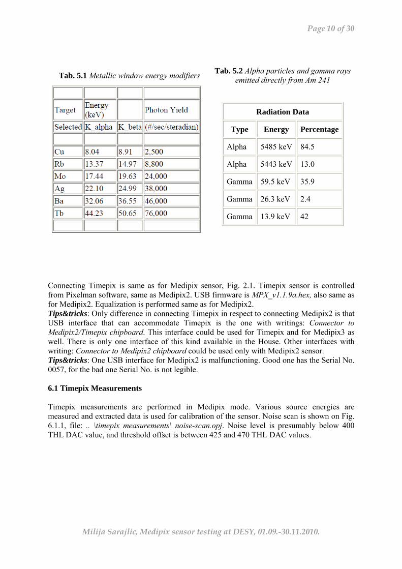
4.1 Medipix2 in energy window mode Medipix2 sensor has also ability to function in so called Energy Window mode. It has implemented two thresholds, THL or low threshold, and THH or high threshold. When THH is lower than THL than Medipix2 operates in Single Threshold mode. If THH is higher than THL, Medipix2 would operate in Energy Window mode. This means that only photons that have energy in the range between THL and THH will be counted towards total count. To test this I took Tb source and swept THH from 400 to 800 THH DAC values. THL was kept constant at value 321 THL DAC. This value for THL was taken as the lowest before sensor starts to see its own noise. Fig. 4.1.1 (file: THH scan.opj) gives total count dependence on the position of the THH. Prominent minimum is visible, which means narrowest energy window attainable. What is expected knowing Medipix2 manual is that total count will go down as THH values goes up to certain value. After point where THH and THL correspond to the same energy, Medipix2 should switch to the Single Threshold mode and we would expect that the total count will rise abruptly to the Single Threshold value. Instead this transition takes some THH values to complete, Fig. 4.1.1. Position of the narrowest energy window is determined at 665 THH DAC. 5. Radioactive source Source is made out of Am 241 with metallic window modifiers with materials: Cu, Rb, Mo, Ag, Ba and Tb. These materials give different energy gamma rays according to the Tab. 5.1 and Tab. 5.2. More detailed data could be found in Ref. [5] or at the web: http://xdb.lbl.gov.

Fig. 4.2 DAC Control Panel window

Fig. 4.3 DAC Dependency Scan window

Fig. 4.4 THL[V] vs. THL DAC values scan

Fig. 4.5 Rb Count vs. THL DAC values

of 30


Fig. 4.1.1 THH scan for Tb source and 10 sec acquisition time.

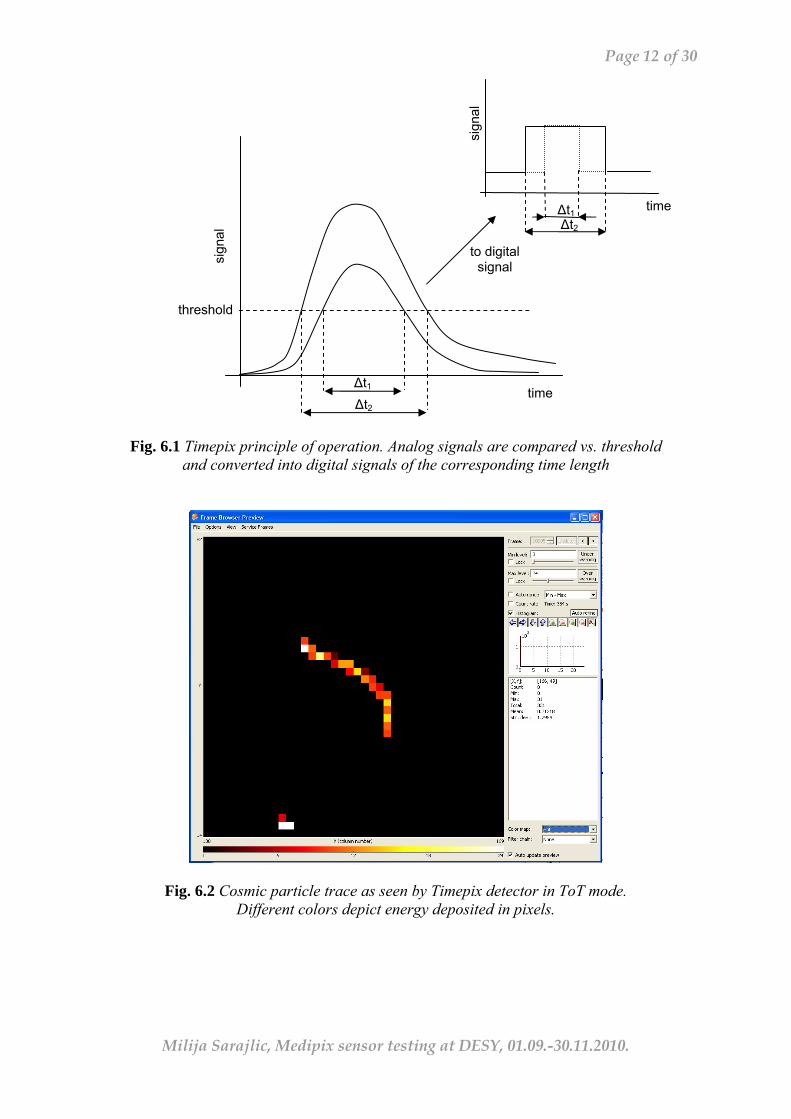
THL value was 321 DAC. 5.1 Source spectrum measurements by Instrument Amptek PX4 More data on Amptek PX4 could be located on the web: http://www.amptek.com/px4.html, or in the manual, file: PX4 Specifications.pdf. Spectrum is measured for all different sources available at Am241 original source. Calibration is performed according to the Ref. [5] and respective plots are given in Fig. 5.1.1(a)-(f). Original files are given in folder: ..\source spectrum, files: *.mca. These files are visible by software: ADMCA.exe, folder ..\ADMCA. Considering Fig. 5.1.1 and Fig. 9.5 for the point where Am241 point is depicted we arrive at the understanding that what is recognized in Fig. 9.4 as Am241 59.5keV line is actually a combination of lines at 59.5keV and around 50keV visible at Fig. 5.1.1(a)-(f). Line at 50keV could be result of the Pb escape photon that appears as a consequence of interaction of Am gamma rays and Pb shielding. Pb has a fluorescence line at energy around 10keV, Ref [5]. 6. Timepix Timepix is based on Medipix2 architecture with added timer. This sensor can operate in various modes: Medipix mode (giving the same functionality as Medipix2 sensor), Time Over Threshold (ToT mode), and First Hit mode. Time over threshold mode measures time that voltage from preamplifier is above threshold, Fig. 6.1. First hit mode measures time when particle hits the pixel. Detailed explanation of Timepix operation is found in Ref [6]. Nice presentation on utilizing Timepix in scientific measurements is given in Ref [7]. Nice example of Timepix in ToT mode is cosmic particle trace, Fig. 6.2. Different colors depict different energy deposited in adjacent pixels. This is also a good example of charge sharing phenomena. Various frames taken by Timepix in different modes are collected in folder: \timepix measurements (.dsc files).

of 30


Tab. 5.1 Metallic window energy modifiers Tab. 5.2 Alpha particles and gamma rays emitted directly from Am 241

Radiation Data

Type Energy Percentage

Alpha 5485 keV 84.5

Alpha 5443 keV 13.0

Gamma 59.5 keV 35.9

Gamma 26.3 keV 2.4

Gamma 13.9 keV 42

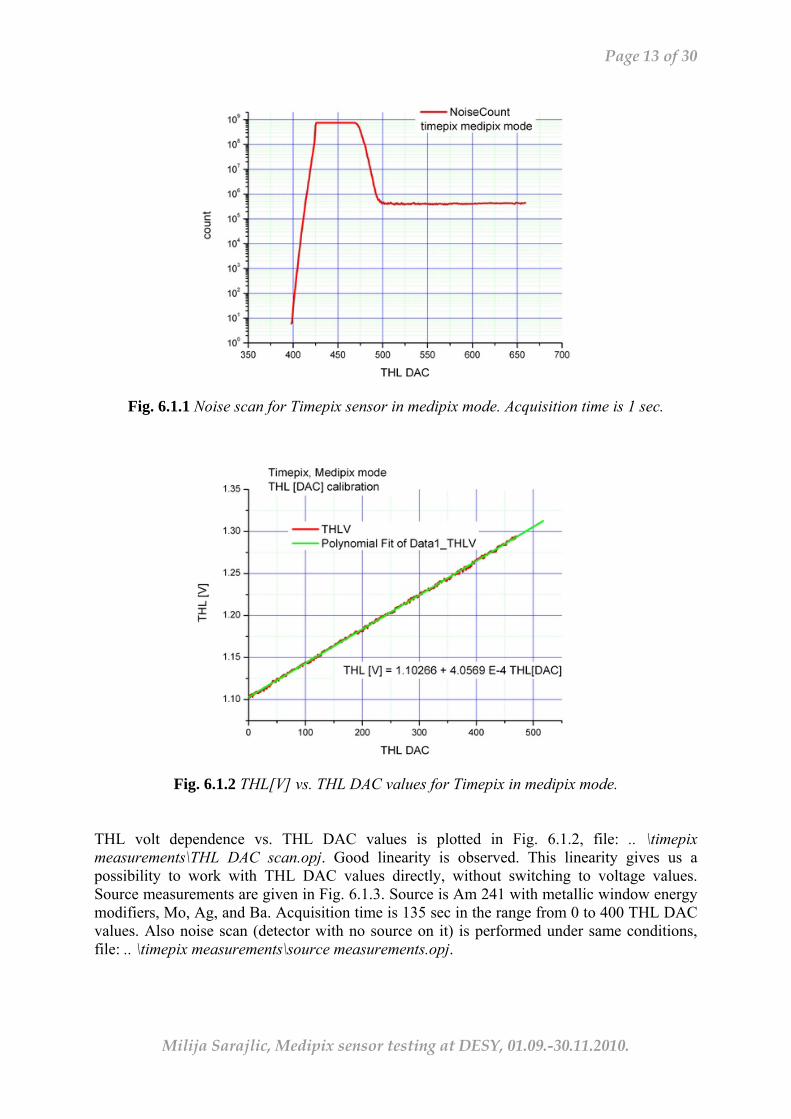
Connecting Timepix is same as for Medipix sensor, Fig. 2.1. Timepix sensor is controlled from Pixelman software, same as Medipix2. USB firmware is MPX_v1.1.9a.hex, also same as for Medipix2. Equalization is performed same as for Medipix2. Tips&tricks: Only difference in connecting Timepix in respect to connecting Medipix2 is that USB interface that can accommodate Timepix is the one with writings: Connector to Medipix2/Timepix chipboard. This interface could be used for Timepix and for Medipix3 as well. There is only one interface of this kind available in the House. Other interfaces with writing: Connector to Medipix2 chipboard could be used only with Medipix2 sensor. Tips&tricks: One USB interface for Medipix2 is malfunctioning. Good one has the Serial No. 0057, for the bad one Serial No. is not legible. 6.1 Timepix Measurements Timepix measurements are performed in Medipix mode. Various source energies are measured and extracted data is used for calibration of the sensor. Noise scan is shown on Fig. 6.1.1, file: .. \timepix measurements\ noise-scan.opj. Noise level is presumably below 400 THL DAC value, and threshold offset is between 425 and 470 THL DAC values.

of 30


(a) (b)

(c) (d)

(e) (f) Fig. 5.1.1 Energy spectrum of various materials exited by Am241

Energy [keV] 10.65 22.85 35.05 47.25

Tb

Rel

ativ

e In

tens

ity

59.26

11.40 23.51 35.61 47.71 59.62

Rel

ativ

e In

tens

ity

Energy [keV]

Cu

Energy [keV] 11.16 23.69 36.76 49.56 62.36

Rb

Rel

ativ

e In

tens

ity

Energy [keV] 10.92 23.35 35.97 48.60 61.22

Mo

Rel

ativ

e In

tens

ity

10.83 23.18 35.72 48.26 Energy [keV]

60.81

Ag

Rel

ativ

e In

tens

ity

Energy [keV] 10.66 23.02 35.38 47.75

Ba

Rel

ativ

e In

tens

ity

59.92

of 30


Fig. 6.1 Timepix principle of operation. Analog signals are compared vs. threshold

and converted into digital signals of the corresponding time length

Fig. 6.2 Cosmic particle trace as seen by Timepix detector in ToT mode. Different colors depict energy deposited in pixels.

time

sign

al

threshold

Δt1 Δt2

time

sign

al

Δt1Δt2

to digital signal

of 30


Fig. 6.1.1 Noise scan for Timepix sensor in medipix mode. Acquisition time is 1 sec.

Fig. 6.1.2 THL[V] vs. THL DAC values for Timepix in medipix mode.

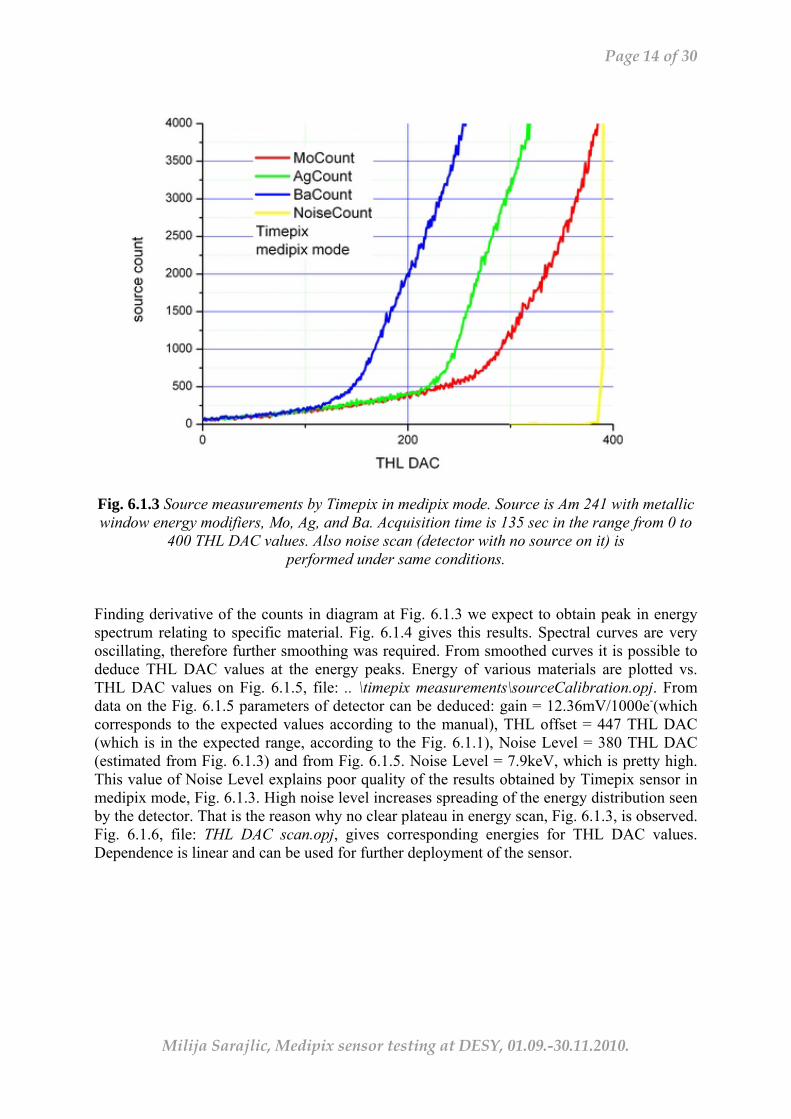
THL volt dependence vs. THL DAC values is plotted in Fig. 6.1.2, file: .. \timepix measurements\THL DAC scan.opj. Good linearity is observed. This linearity gives us a possibility to work with THL DAC values directly, without switching to voltage values. Source measurements are given in Fig. 6.1.3. Source is Am 241 with metallic window energy modifiers, Mo, Ag, and Ba. Acquisition time is 135 sec in the range from 0 to 400 THL DAC values. Also noise scan (detector with no source on it) is performed under same conditions, file: .. \timepix measurements\source measurements.opj.

of 30


Fig. 6.1.3 Source measurements by Timepix in medipix mode. Source is Am 241 with metallic window energy modifiers, Mo, Ag, and Ba. Acquisition time is 135 sec in the range from 0 to

400 THL DAC values. Also noise scan (detector with no source on it) is performed under same conditions.

Finding derivative of the counts in diagram at Fig. 6.1.3 we expect to obtain peak in energy spectrum relating to specific material. Fig. 6.1.4 gives this results. Spectral curves are very oscillating, therefore further smoothing was required. From smoothed curves it is possible to deduce THL DAC values at the energy peaks. Energy of various materials are plotted vs. THL DAC values on Fig. 6.1.5, file: .. \timepix measurements\sourceCalibration.opj. From data on the Fig. 6.1.5 parameters of detector can be deduced: gain = 12.36mV/1000e-(which corresponds to the expected values according to the manual), THL offset = 447 THL DAC (which is in the expected range, according to the Fig. 6.1.1), Noise Level = 380 THL DAC (estimated from Fig. 6.1.3) and from Fig. 6.1.5. Noise Level = 7.9keV, which is pretty high. This value of Noise Level explains poor quality of the results obtained by Timepix sensor in medipix mode, Fig. 6.1.3. High noise level increases spreading of the energy distribution seen by the detector. That is the reason why no clear plateau in energy scan, Fig. 6.1.3, is observed. Fig. 6.1.6, file: THL DAC scan.opj, gives corresponding energies for THL DAC values. Dependence is linear and can be used for further deployment of the sensor.

of 30


Fig. 6.1.4 Derivate of the sensor count for different materials. Curves are very oscilating,

therefore smoothing is performed. From here, corresponding source energy THL DAC values are extracted.

Fig. 6.1.5 Source energy calibration. Timepix medipix mode.

of 30


Fig. 6.1.6 Threshold DAC values calibration for Medipix in timepix mode

7. Medipix3 Medipix3 has additional feature in respect to the Medipix2 or Timepix, it is capable of operating in Charge Summing mode. This mode is meant to reduce or totally diminish effect of charge sharing. Implementation of this mode of operation is given in Ref. [8]. Details on Medipix3 construction are given in manual, Ref [9]. Nice presentation on the first measurements performed with Medipix3 is given in Ref. [12]. Medipix connection to USB interface is given in Fig. 7.1, file: Medipix3-connecting.JPG. USB interface in this connection scheme is turned on the back side.

Fig. 7.1 Schematics of Medipix3 connection. Pay attention that USB is turned on the back side.

of 30


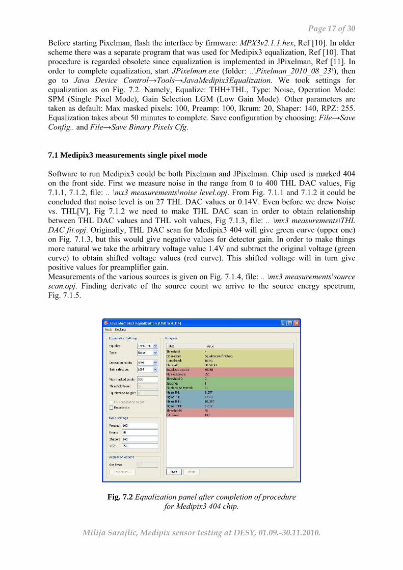
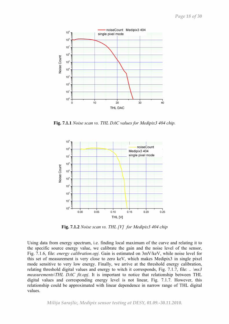
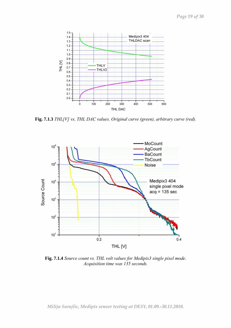
Before starting Pixelman, flash the interface by firmware: MPX3v2.1.1.hex, Ref [10]. In older scheme there was a separate program that was used for Medipix3 equalization, Ref [10]. That procedure is regarded obsolete since equalization is implemented in JPixelman, Ref [11]. In order to complete equalization, start JPixelman.exe (folder: ..\Pixelman_2010_08_23\), then go to Java Device Control→Tools→JavaMedipix3Equalization. We took settings for equalization as on Fig. 7.2. Namely, Equalize: THH+THL, Type: Noise, Operation Mode: SPM (Single Pixel Mode), Gain Selection LGM (Low Gain Mode). Other parameters are taken as default: Max masked pixels: 100, Preamp: 100, Ikrum: 20, Shaper: 140, RPZ: 255. Equalization takes about 50 minutes to complete. Save configuration by choosing: File→Save Config.. and File→Save Binary Pixels Cfg. 7.1 Medipix3 measurements single pixel mode Software to run Medipix3 could be both Pixelman and JPixelman. Chip used is marked 404 on the front side. First we measure noise in the range from 0 to 400 THL DAC values, Fig 7.1.1, 7.1.2, file: .. \mx3 measurements\noise level.opj. From Fig. 7.1.1 and 7.1.2 it could be concluded that noise level is on 27 THL DAC values or 0.14V. Even before we drew Noise vs. THL[V], Fig 7.1.2 we need to make THL DAC scan in order to obtain relationship between THL DAC values and THL volt values, Fig 7.1.3, file: .. \mx3 measurements\THL DAC fit.opj. Originally, THL DAC scan for Medipix3 404 will give green curve (upper one) on Fig. 7.1.3, but this would give negative values for detector gain. In order to make things more natural we take the arbitrary voltage value 1.4V and subtract the original voltage (green curve) to obtain shifted voltage values (red curve). This shifted voltage will in turn give positive values for preamplifier gain. Measurements of the various sources is given on Fig. 7.1.4, file: .. \mx3 measurements\source scan.opj. Finding derivate of the source count we arrive to the source energy spectrum, Fig. 7.1.5.

Fig. 7.2 Equalization panel after completion of procedure for Medipix3 404 chip.

of 30


Fig. 7.1.1 Noise scan vs. THL DAC values for Medipix3 404 chip.

Fig. 7.1.2 Noise scan vs. THL [V] for Medipix3 404 chip

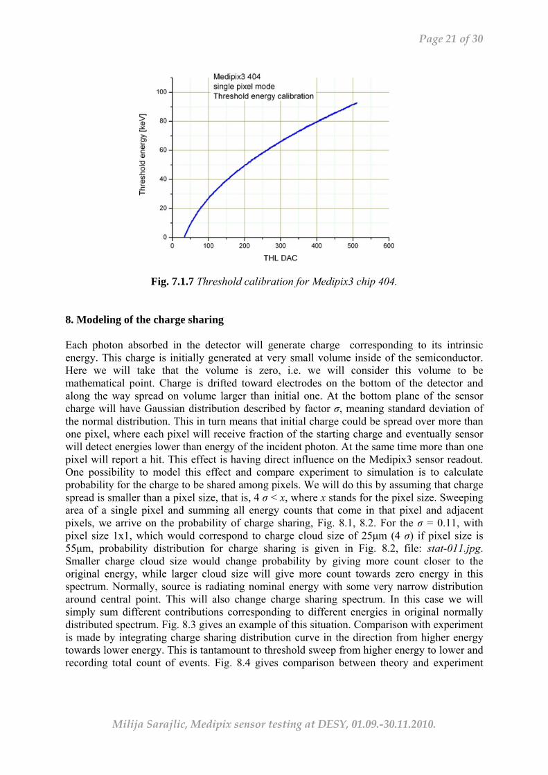
Using data from energy spectrum, i.e. finding local maximum of the curve and relating it to the specific source energy value, we calibrate the gain and the noise level of the sensor, Fig. 7.1.6, file: energy calibration.opj. Gain is estimated on 3mV/keV, while noise level for this set of measurement is very close to zero keV, which makes Medipix3 in single pixel mode sensitive to very low energy. Finally, we arrive at the threshold energy calibration, relating threshold digital values and energy to witch it corresponds, Fig. 7.1.7, file: .. \mx3 measurements\THL DAC fit.opj. It is important to notice that relationship between THL digital values and corresponding energy level is not linear, Fig. 7.1.7. However, this relationship could be approximated with linear dependence in narrow range of THL digital values.

of 30


Fig. 7.1.3 THL[V] vs. THL DAC values. Original curve (green), arbitrary curve (red).

Fig. 7.1.4 Source count vs. THL volt values for Medipix3 single pixel mode.

Acquisition time was 135 seconds.

of 30


Fig. 7.1.5 Source count derivative vs. voltage values of THL. Shifted peaks are visible

on different voltage values for different sources.

Fig. 7.1.6 Energy calibration Medipix3, chip 404. Gain: 3mV/keV (arbitrary), noise level = 0keV(!)

of 30


Fig. 7.1.7 Threshold calibration for Medipix3 chip 404.

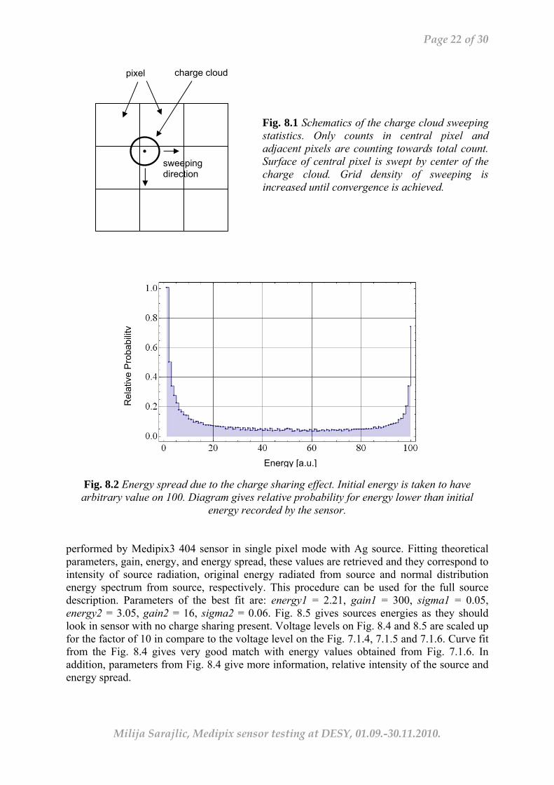
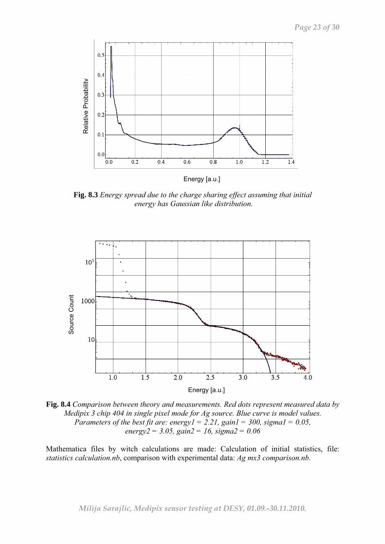
8. Modeling of the charge sharing Each photon absorbed in the detector will generate charge corresponding to its intrinsic energy. This charge is initially generated at very small volume inside of the semiconductor. Here we will take that the volume is zero, i.e. we will consider this volume to be mathematical point. Charge is drifted toward electrodes on the bottom of the detector and along the way spread on volume larger than initial one. At the bottom plane of the sensor charge will have Gaussian distribution described by factor σ, meaning standard deviation of the normal distribution. This in turn means that initial charge could be spread over more than one pixel, where each pixel will receive fraction of the starting charge and eventually sensor will detect energies lower than energy of the incident photon. At the same time more than one pixel will report a hit. This effect is having direct influence on the Medipix3 sensor readout. One possibility to model this effect and compare experiment to simulation is to calculate probability for the charge to be shared among pixels. We will do this by assuming that charge spread is smaller than a pixel size, that is, 4 σ < x, where x stands for the pixel size. Sweeping area of a single pixel and summing all energy counts that come in that pixel and adjacent pixels, we arrive on the probability of charge sharing, Fig. 8.1, 8.2. For the σ = 0.11, with pixel size 1x1, which would correspond to charge cloud size of 25μm (4 σ) if pixel size is 55μm, probability distribution for charge sharing is given in Fig. 8.2, file: stat-011.jpg. Smaller charge cloud size would change probability by giving more count closer to the original energy, while larger cloud size will give more count towards zero energy in this spectrum. Normally, source is radiating nominal energy with some very narrow distribution around central point. This will also change charge sharing spectrum. In this case we will simply sum different contributions corresponding to different energies in original normally distributed spectrum. Fig. 8.3 gives an example of this situation. Comparison with experiment is made by integrating charge sharing distribution curve in the direction from higher energy towards lower energy. This is tantamount to threshold sweep from higher energy to lower and recording total count of events. Fig. 8.4 gives comparison between theory and experiment

of 30


Fig. 8.1 Schematics of the charge cloud sweeping statistics. Only counts in central pixel and adjacent pixels are counting towards total count. Surface of central pixel is swept by center of the charge cloud. Grid density of sweeping is increased until convergence is achieved.

Fig. 8.2 Energy spread due to the charge sharing effect. Initial energy is taken to have arbitrary value on 100. Diagram gives relative probability for energy lower than initial

energy recorded by the sensor. performed by Medipix3 404 sensor in single pixel mode with Ag source. Fitting theoretical parameters, gain, energy, and energy spread, these values are retrieved and they correspond to intensity of source radiation, original energy radiated from source and normal distribution energy spectrum from source, respectively. This procedure can be used for the full source description. Parameters of the best fit are: energy1 = 2.21, gain1 = 300, sigma1 = 0.05, energy2 = 3.05, gain2 = 16, sigma2 = 0.06. Fig. 8.5 gives sources energies as they should look in sensor with no charge sharing present. Voltage levels on Fig. 8.4 and 8.5 are scaled up for the factor of 10 in compare to the voltage level on the Fig. 7.1.4, 7.1.5 and 7.1.6. Curve fit from the Fig. 8.4 gives very good match with energy values obtained from Fig. 7.1.6. In addition, parameters from Fig. 8.4 give more information, relative intensity of the source and energy spread.

Energy [a.u.]

Rel

ativ

e Pr

obab

ility

pixel charge cloud

sweeping direction

of 30


Fig. 8.3 Energy spread due to the charge sharing effect assuming that initial

energy has Gaussian like distribution.

Fig. 8.4 Comparison between theory and measurements. Red dots represent measured data by

Medipix 3 chip 404 in single pixel mode for Ag source. Blue curve is model values. Parameters of the best fit are: energy1 = 2.21, gain1 = 300, sigma1 = 0.05,

energy2 = 3.05, gain2 = 16, sigma2 = 0.06 Mathematica files by witch calculations are made: Calculation of initial statistics, file: statistics calculation.nb, comparison with experimental data: Ag mx3 comparison.nb.

Energy [a.u.]

Sou

rce

Cou

nt

Energy [a.u.]

Rel

ativ

e P

roba

bilit

y

of 30


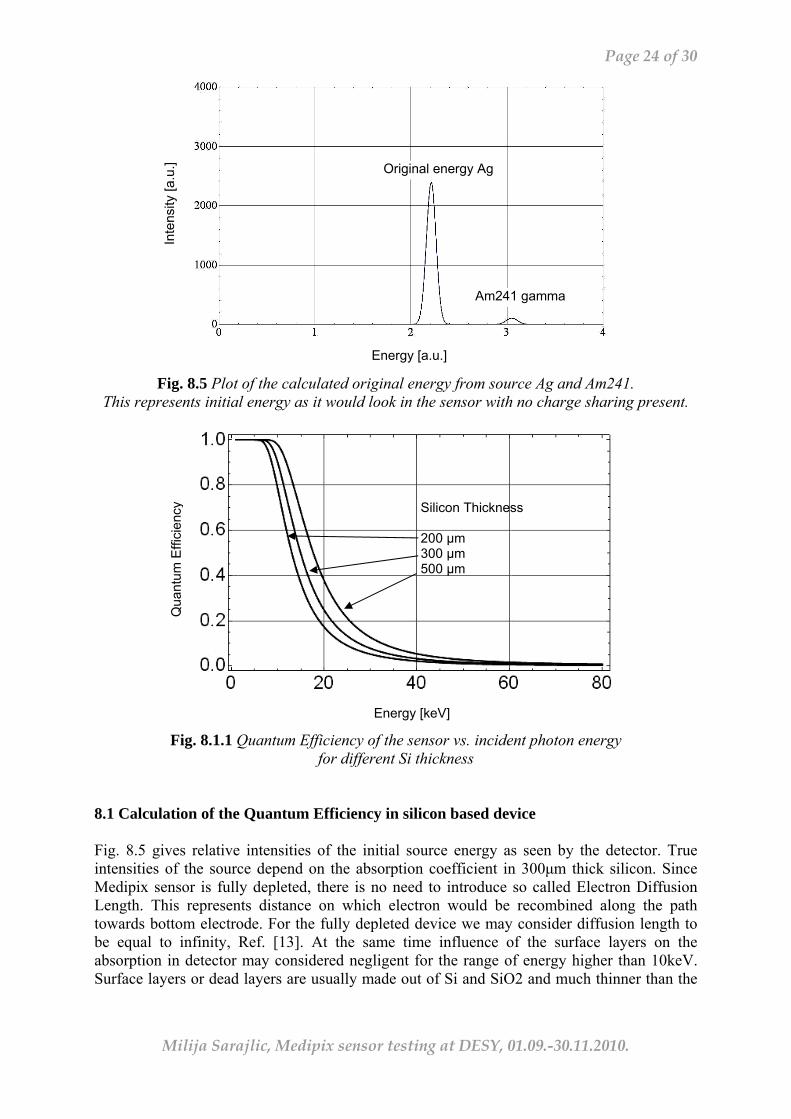
Fig. 8.5 Plot of the calculated original energy from source Ag and Am241.

This represents initial energy as it would look in the sensor with no charge sharing present.

Fig. 8.1.1 Quantum Efficiency of the sensor vs. incident photon energy

for different Si thickness 8.1 Calculation of the Quantum Efficiency in silicon based device Fig. 8.5 gives relative intensities of the initial source energy as seen by the detector. True intensities of the source depend on the absorption coefficient in 300μm thick silicon. Since Medipix sensor is fully depleted, there is no need to introduce so called Electron Diffusion Length. This represents distance on which electron would be recombined along the path towards bottom electrode. For the fully depleted device we may consider diffusion length to be equal to infinity, Ref. [13]. At the same time influence of the surface layers on the absorption in detector may considered negligent for the range of energy higher than 10keV. Surface layers or dead layers are usually made out of Si and SiO2 and much thinner than the

Energy [keV]

Qua

ntum

Effi

cien

cy

Silicon Thickness 200 μm 300 μm 500 μm

Energy [a.u.]

Inte

nsity

[a.u

.] Original energy Ag

Am241 gamma

of 30


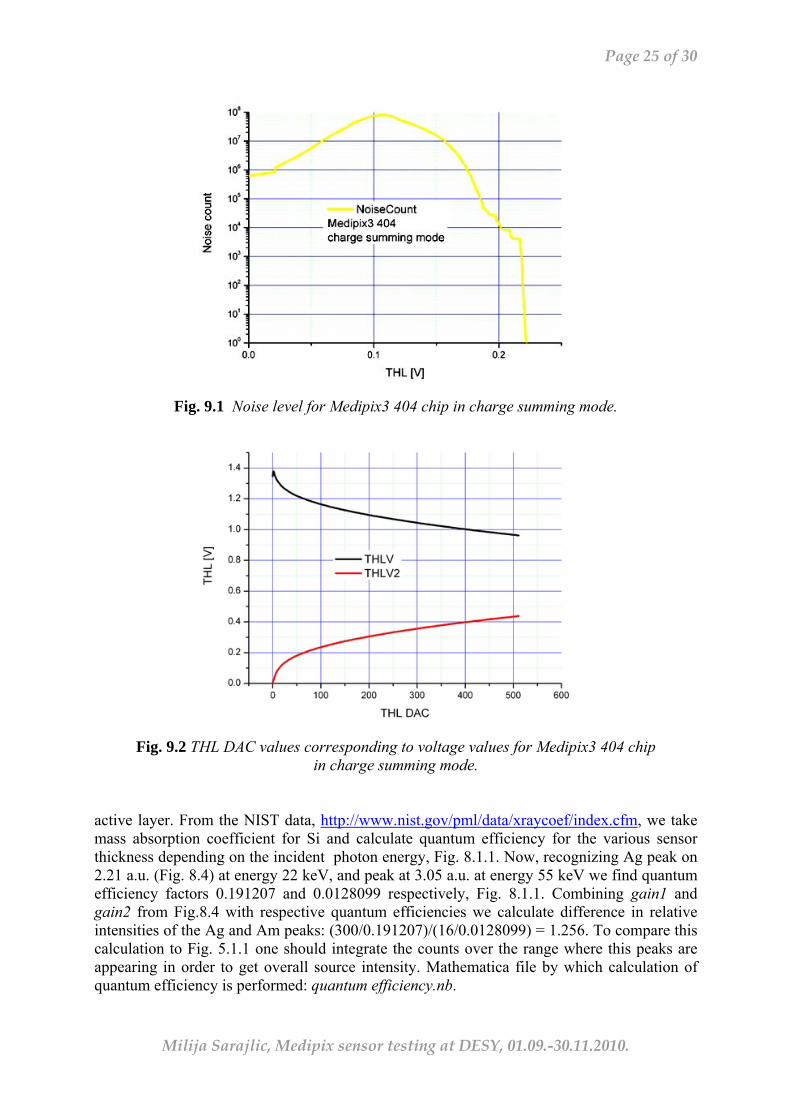
Fig. 9.1 Noise level for Medipix3 404 chip in charge summing mode.

Fig. 9.2 THL DAC values corresponding to voltage values for Medipix3 404 chip

in charge summing mode. active layer. From the NIST data, http://www.nist.gov/pml/data/xraycoef/index.cfm, we take mass absorption coefficient for Si and calculate quantum efficiency for the various sensor thickness depending on the incident photon energy, Fig. 8.1.1. Now, recognizing Ag peak on 2.21 a.u. (Fig. 8.4) at energy 22 keV, and peak at 3.05 a.u. at energy 55 keV we find quantum efficiency factors 0.191207 and 0.0128099 respectively, Fig. 8.1.1. Combining gain1 and gain2 from Fig.8.4 with respective quantum efficiencies we calculate difference in relative intensities of the Ag and Am peaks: (300/0.191207)/(16/0.0128099) = 1.256. To compare this calculation to Fig. 5.1.1 one should integrate the counts over the range where this peaks are appearing in order to get overall source intensity. Mathematica file by which calculation of quantum efficiency is performed: quantum efficiency.nb.

of 30


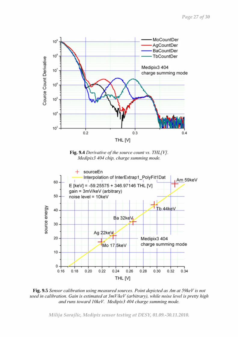
9. Medipix3 measurements charge summing mode Medipix can be operated only in modes: Single pixel full sequential mode and Charge summing full sequential mode, Ref [9]. By default it is positioned in the single pixel mode. To change the mode of operation go to: Tools→Specific Acquisition Settings and in a drop down list change settings to Charge summing full sequential mode. Threshold equalization needs to be performed separately for charge summing mode, file: 03-11-10-thl+thh equalize.png. Settings for equalization we used are the same as in the case of single pixel mode with the only difference that Operation Mode: CSM (Charge Summing Mode). equalization took significantly more time than in the case of the single pixel mode, more than six hours to complete. Noise scan of Medipix3 404 chip in charge summing mode is given in Fig. 9.1. Noise appears higher than in single pixel mode, Fig. 7.1.2. THL DAC values scan is given in Fig. 9.2. Measured count values for different materials is given in Fig. 9.3. Derivate values for counts with corresponding peaks given in Fig. 9.4. Sensor calibration in respect to the measured values, Fig. 9.5. Gain is estimated at 3mV/keV (arbitrary), while noise level is pretty high and runs toward 10keV. Final calibration of THL DAC values towards threshold energy is given in Fig. 9.6. Origin files of the measurements are in the folder: ..\mx3 measurements\charge summing, (files: .opj).

Fig. 9.3 Source count for various materials vs. THL voltage values.

Medipix3 404 chip, charge summing mode.

of 30


Fig. 9.4 Derivative of the source count vs. THL[V].

Medipix3 404 chip, charge summing mode.

Fig. 9.5 Sensor calibration using measured sources. Point depicted as Am at 59keV is not

used in calibration. Gain is estimated at 3mV/keV (arbitrary), while noise level is pretty high and runs toward 10keV. Medipix3 404 charge summing mode.

of 30


Fig. 9.6 Calibration of the Medipix3 THL DAC values to corresponding

threshold energy.

10. Taking images with Medipix3 in Single Pixel mode Metallic nut, M3 (5mm across) is attached close to the Medipix3 404 chip sensor and irradiated by Tb source (from Am241), Fig. 10.1. Acquisition was more than 2.5 hours. Good contrast and visibility is achieved. Tb source is chosen because of the high intensity that it gives. Pixelman frame with this measurement is: ..\mx3 measurements\nut--01.txt.dsc. The nut looks larger on this photo because it could not be placed exactly on the surface of the detector and therefore shadow that is recorded looks bigger than original object. 10.1 Taking images with Medipix2 in Energy Window mode Energy Window mode was chosen for the possibility to filter out lower energy x-rays. From the previous measurements it is not possible at this point to say which range of energy we are scanning with, but I would suppose that it relates to energy around 10keV. THL value is set to 321 DAC which would give lowest threshold level before sensor noise would start to appear. THH value is set to 665 DAC corresponding to the narrowest energy window, Fig. 4.1.1. Object scanned is chip (integrated circuitry). Source used is Tb exited by Am241. Integration time was more than 22 hours. Fig. 10.1.1 depicts this image. Visible are the pins of the chip and the holder for the chip itself.

of 30


Fig. 10.1 Pixelman frame of the metallic nut photo taken by Medipix3 404 chip in the single pixel mode. Source was Tb and acquisition time close to 2.5 hours.

Fig. 10.1.1 Chip scan recorded by Medipix2 in Energy Window mode

of 30


References [1] Medipix2 manual, file: manual-Mpix2MXR20 Documentv2.3.pdf. [2] Lawrence Pinsky, “Application of the Medipix2 Technology to Space Radiation

Dosymetry and Hadron Therapy Beam Monitoring”, Viena Conference on Instrumentation, February 20. 2010, file: application of the medipix2 technology.pdf

[3] C. Teyssier, J. Bouchami, F. Dallaire, J. Idarraga, C. Leroy, S. Pospisil, J. Solc, O. Scallon, Z. Vykydal, “Performance of the Medipix and Timepix devices for the recognition of electron-gamma radiation fields”, PIXEL2010, file: Performance of the Medipix.pdf

[4] S. Eidelman et al., Physics Letters B592, 1 (2004), file: PASSAGE OF PARTICLES THROUGH MATTER.pdf

[5] Albert Thompson et al. “X-ray data booklet”, Lawrence Berkeley National Laboratory, University of California, Berkeley, CA 94720.

[6] Xavier Llopart, “Timepix Manual v1.0”, file: Timepix Manual v1.0.pdf [7] Veerle Heijne, “Timepix a pixel detector for the future”, Amsterdam Master of Physics

Symposium, 16, April 2010, file: Timepix a pixel detector for the future.pdf [8] R. Ballabriga, M. Campbell, E. H. M. Heijne, X. Llopart, L. Tlustos, “The Medipix3

Prototype, a Pixel Readout Chip Working in Single Photon Counting Mode with Improved Spectrometric Performance”, Nuclear Science Symposium Conference Record, San Diego CA, 2006. IEEE, pp. 3557 - 3561, October 29. 2006. - November 1. 2006., doi: 10.1109/NSSMIC.2006.353767 file: MEDIPIX3_NSS-MIC06_Transactions.pdf.

[9] Medipix3 manual, file: Medipix3manualv19.pdf [10] Old procedure Medipix3 equalization, file: medipix3equalization-old.pdf [11] Equalizing Medipix3, file: equalizing medipix3 pixelman.pdf [12] X. Llopart, R. Ballabriga, W. Wong, D. Turecek, T. Tlustos, ”MEDIPIX3 TESTING

STATUS”, file: MEDIPIX3 TESTING STATUS-19-11-2009.pdf [13] M.C.Peckerar, W.D.Baker, and D.J.Nagel, “X-ray sensitivity of a charge-coupled-

device array”, Journal of Applied Physics, Vol. 48, No.6, June 1977, file: X-ray sensitivity of a charge-coupled-device array.pdf

Medipix calibration experiments and theory MSarajlic -...

Documents

Transcript of Medipix calibration experiments and theory MSarajlic -...