1

Mechanics of Solids

notes

2

UNIT-III

Deflection of Beams

Deflection of Beams

Introduction:

In all practical engineering applications, when we use the different components,

normally we have to operate them within the certain limits i.e. the constraints are

placed on the performance and behavior of the components. For instance we say

that the particular component is supposed to operate within this value of stress and

the deflection of the component should not exceed beyond a particular value.

In some problems the maximum stress however, may not be a strict or severe

condition but there may be the deflection which is the more rigid condition under

operation. It is obvious therefore to study the methods by which we can predict the

deflection of members under lateral loads or transverse loads, since it is this form of

loading which will generally produce the greatest deflection of beams.

Assumption: The following assumptions are undertaken in order to derive a

differential equation of elastic curve for the loaded beam

1. Stress is proportional to strain i.e. hooks law applies. Thus, the equation is valid

only for beams that are not stressed beyond the elastic limit.

2. The curvature is always small.

3. Any deflection resulting from the shear deformation of the material or shear

stresses is neglected.

It can be shown that the deflections due to shear deformations are usually small and

hence can be ignored.

3

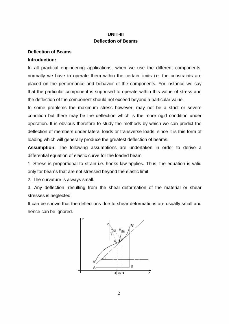
Consider a beam AB which is initially straight and horizontal when unloaded. If under

the action of loads the beam deflect to a position A'B' under load or infact we say

that the axis of the beam bends to a shape A'B'. It is customary to call A'B' the

curved axis of the beam as the elastic line or deflection curve.

In the case of a beam bent by transverse loads acting in a plane of symmetry, the

bending moment M varies along the length of the beam and we represent the

variation of bending moment in B.M diagram. Futher, it is assumed that the simple

bending theory equation holds good.

If we look at the elastic line or the deflection curve, this is obvious that the curvature

at every point is different; hence the slope is different at different points.

To express the deflected shape of the beam in rectangular co-ordinates let us take

two axes x and y, x-axis coincide with the original straight axis of the beam and the y

– axis shows the deflection.

Futher,let us consider an element ds of the deflected beam. At the ends of this

element let us construct the normal which intersect at point O denoting the angle

between these two normal be di

But for the deflected shape of the beam the slope i at any point C is defined,

4

This is the differential equation of the elastic line for a beam subjected to bending in

the plane of symmetry. Its solution y = f(x) defines the shape of the elastic line or the

deflection curve as it is frequently called.

Relationship between shear force, bending moment and deflection: The

relationship among shear force,bending moment and deflection of the beam may be

obtained as

Differentiating the equation as derived

Therefore, the above expression represents the shear force whereas rate of intensity

of loading can also be found out by differentiating the expression for shear force

Methods for finding the deflection: The deflection of the loaded beam can be

obtained various methods.The one of the method for finding the deflection of the

beam is the direct integration method, i.e. the method using the differential equation

which we have derived.

Direct integration method: The governing differential equation is defined as

5

Where A and B are constants of integration to be evaluated from the known

conditions of slope and deflections for the particular value of x.

Illustrative examples : let us consider few illustrative examples to have a familiarty

with the direct integration method

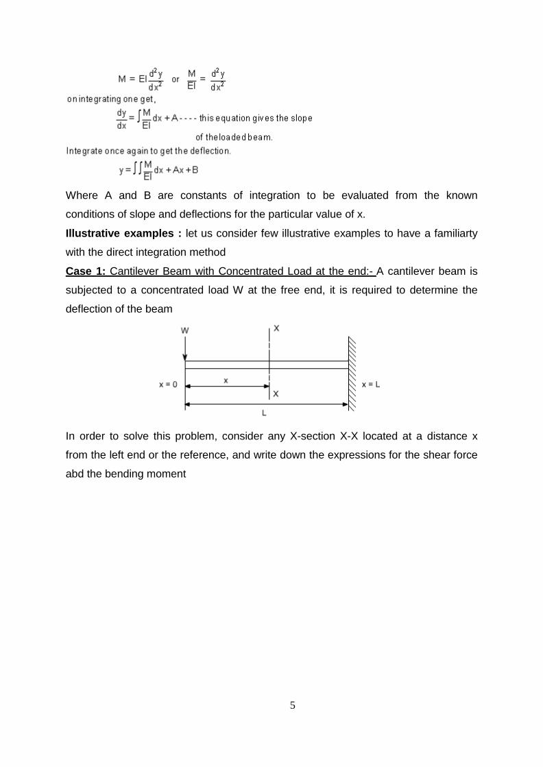
Case 1: Cantilever Beam with Concentrated Load at the end:- A cantilever beam is

subjected to a concentrated load W at the free end, it is required to determine the

deflection of the beam

In order to solve this problem, consider any X-section X-X located at a distance x

from the left end or the reference, and write down the expressions for the shear force

abd the bending moment

6

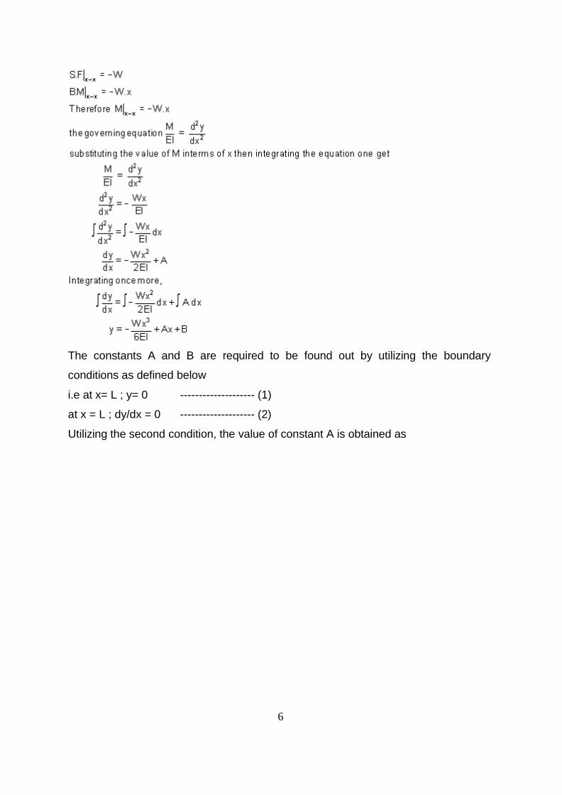
The constants A and B are required to be found out by utilizing the boundary

conditions as defined below

i.e at x= L ; y= 0 -------------------- (1)

at x = L ; dy/dx = 0 -------------------- (2)

Utilizing the second condition, the value of constant A is obtained as

7

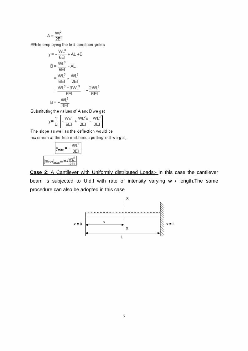
Case 2: A Cantilever with Uniformly distributed Loads:- In this case the cantilever

beam is subjected to U.d.l with rate of intensity varying w / length.The same

procedure can also be adopted in this case

8

Boundary conditions relevant to the problem are as follows:

1. At x = L; y = 0

2. At x= L; dy/dx = 0

The second boundary conditions yields

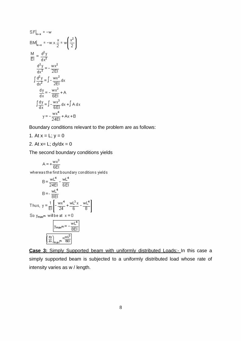
Case 3: Simply Supported beam with uniformly distributed Loads:- In this case a

simply supported beam is subjected to a uniformly distributed load whose rate of

intensity varies as w / length.

9

In order to write down the expression for bending moment consider any cross-

section at distance of x metre from left end support.

Boundary conditions which are relevant in this case are that the deflection at each

support must be zero.

i.e. at x = 0; y = 0 : at x = l; y = 0

let us apply these two boundary conditions on equation (1) because the boundary

conditions are on y, This yields B = 0.

10

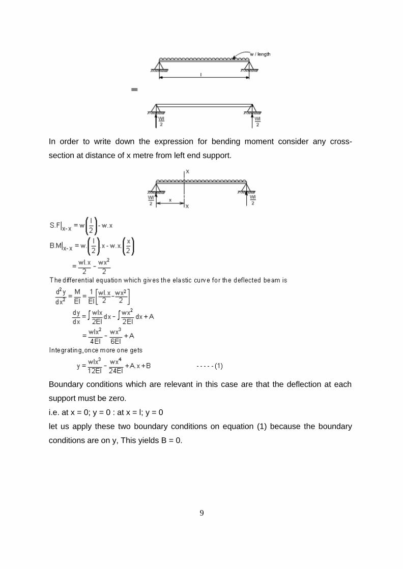
Futher

In this case the maximum deflection will occur at the centre of the beam where x =

L/2 [ i.e. at the position where the load is being applied ].So if we substitute the value

of x = L/2

Conclusions

(i) The value of the slope at the position where the deflection is maximum would be

zero.

(ii) Thevalue of maximum deflection would be at the centre i.e. at x = L/2.

The final equation which is governs the deflection of the loaded beam in this case is

By successive differentiation one can find the relations for slope, bending moment,

shear force and rate of loading.

Deflection (y)

Slope (dy/dx)

Bending Moment So the bending moment diagram would

11

be

Shear Force

Shear force is obtained by

taking

third derivative.

Rate of intensity of

loading

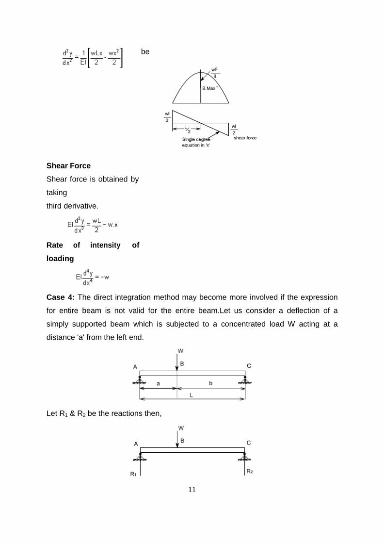
Case 4: The direct integration method may become more involved if the expression

for entire beam is not valid for the entire beam.Let us consider a deflection of a

simply supported beam which is subjected to a concentrated load W acting at a

distance 'a' from the left end.

Let R1 & R2 be the reactions then,

12

These two equations can be integrated in the usual way to find ‘y' but this will result

in four constants of integration two for each equation. To evaluate the four constants

of integration, four independent boundary conditions will be needed since the

deflection of each support must be zero, hence the boundary conditions (a) and (b)

can be realized.

Further, since the deflection curve is smooth, the deflection equations for the same

slope and deflection at the point of application of load i.e. at x = a. Therefore four

conditions required to evaluate these constants may be defined as follows:

(a) at x = 0; y = 0 in the portion AB i.e. 0 ≤ x ≤ a

(b) at x = l; y = 0 in the portion BC i.e. a ≤ x ≤ l

(c) at x = a; dy/dx, the slope is same for both portion

(d) at x = a; y, the deflection is same for both portion

By symmetry, the reaction R1 is obtained as

Using condition (c) in equation (3) and (4) shows that these constants should be

equal, hence letting

K1 = K2 = K

13

Hence

Now lastly k3 is found out using condition (d) in equation (5) and equation (6), the

condition (d) is that,

At x = a; y; the deflection is the same for both portion

14

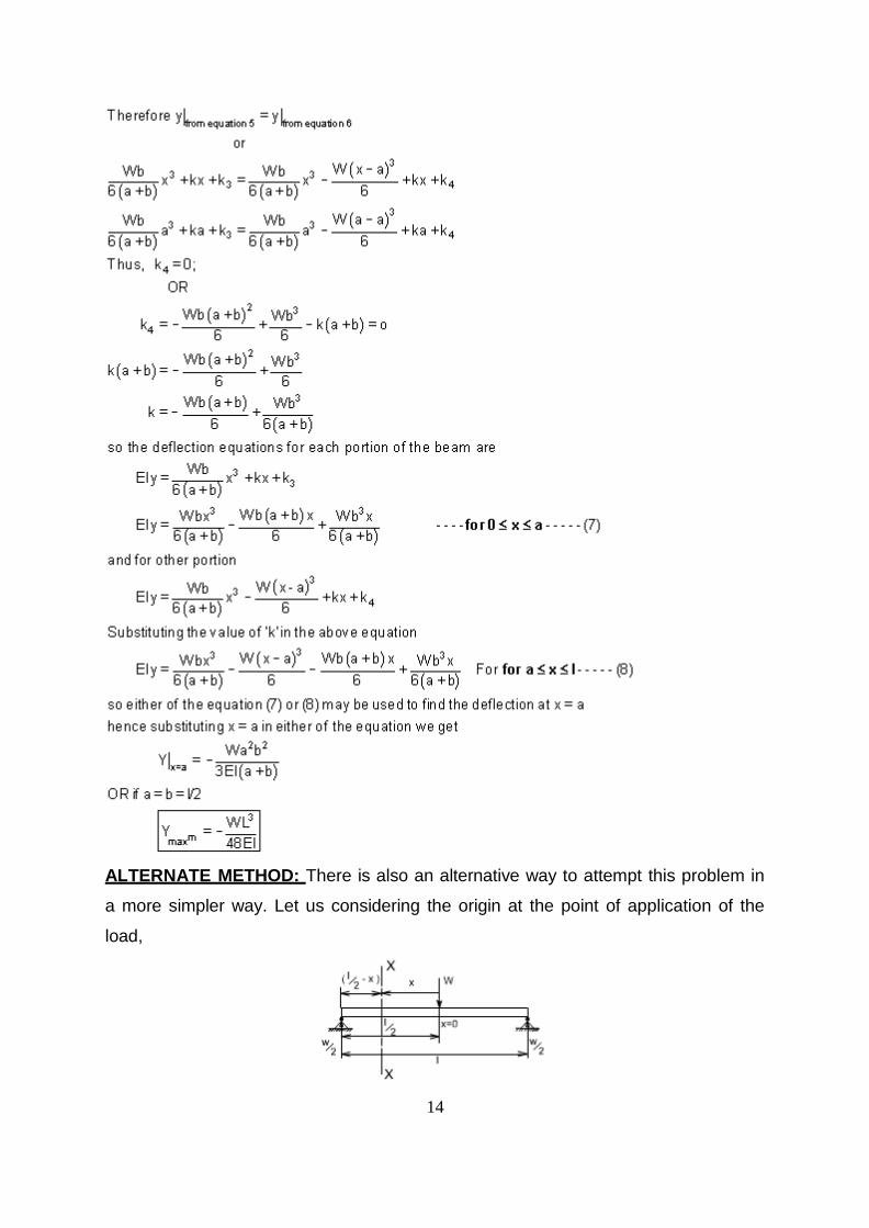
ALTERNATE METHOD: There is also an alternative way to attempt this problem in

a more simpler way. Let us considering the origin at the point of application of the

load,

15

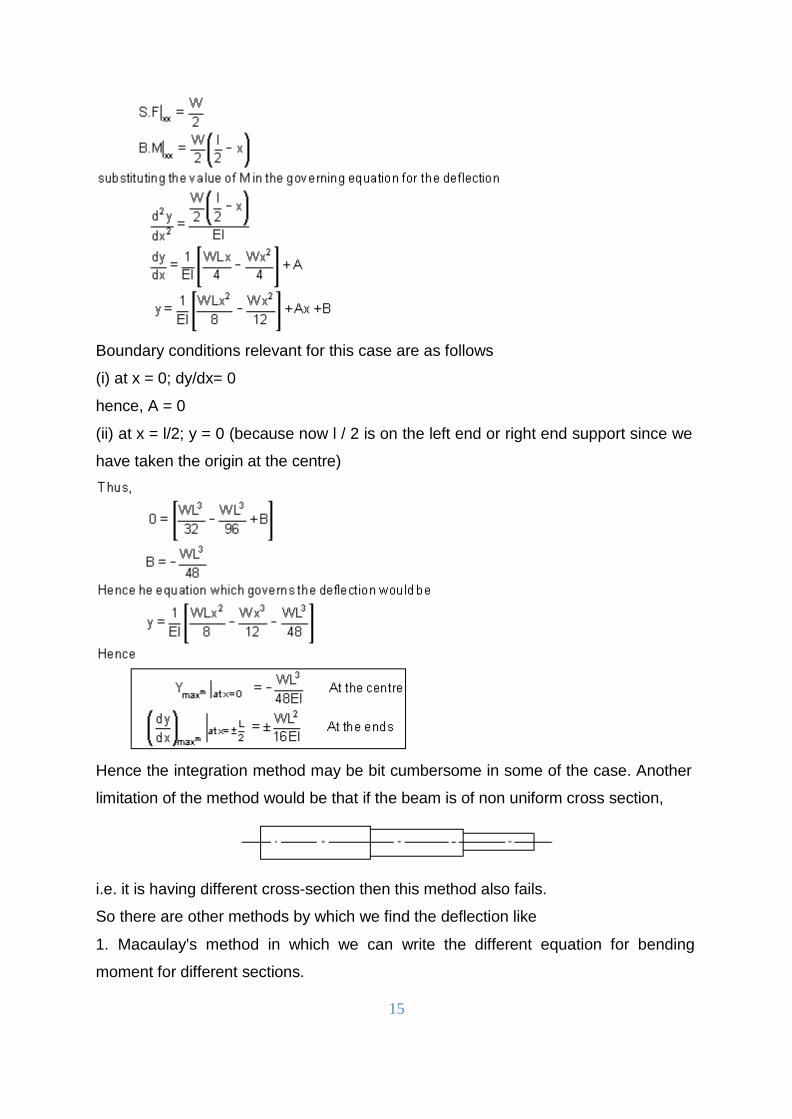
Boundary conditions relevant for this case are as follows

(i) at x = 0; dy/dx= 0

hence, A = 0

(ii) at x = l/2; y = 0 (because now l / 2 is on the left end or right end support since we

have taken the origin at the centre)

Hence the integration method may be bit cumbersome in some of the case. Another

limitation of the method would be that if the beam is of non uniform cross section,

i.e. it is having different cross-section then this method also fails.

So there are other methods by which we find the deflection like

1. Macaulay's method in which we can write the different equation for bending

moment for different sections.

16

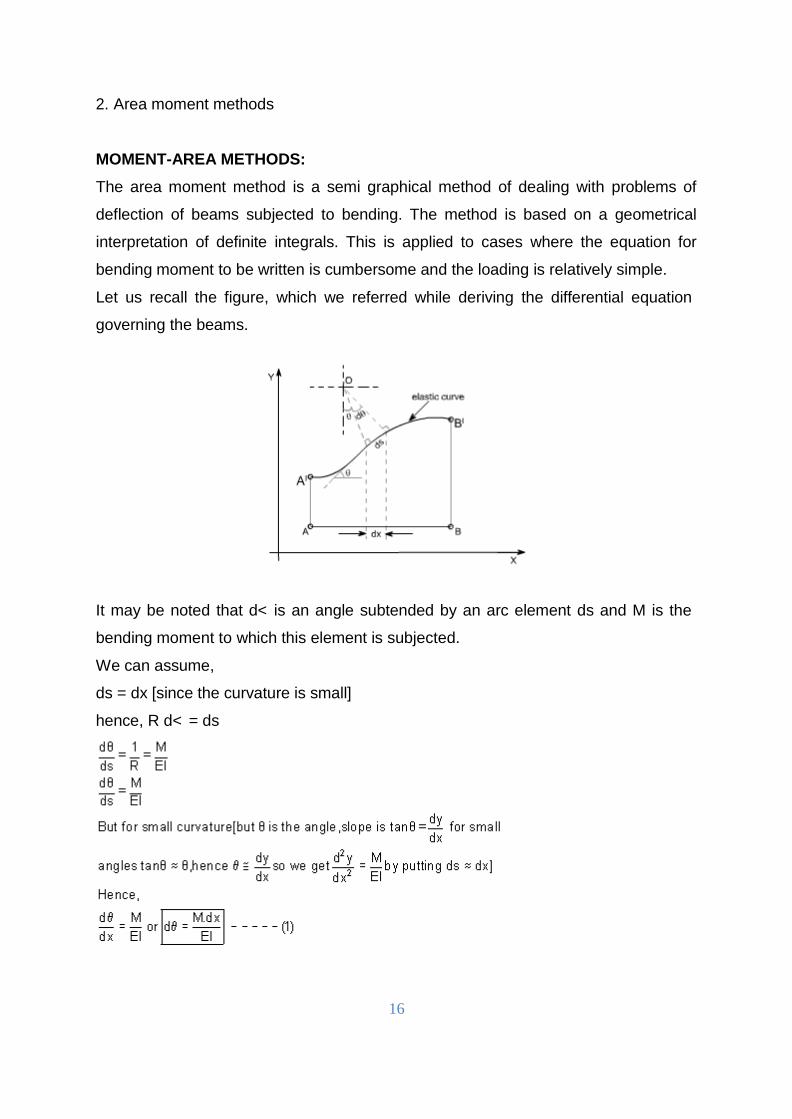
2. Area moment methods MOMENT-AREA METHODS:

The area moment method is a semi graphical method of dealing with problems of

deflection of beams subjected to bending. The method is based on a geometrical

interpretation of definite integrals. This is applied to cases where the equation for

bending moment to be written is cumbersome and the loading is relatively simple.

Let us recall the figure, which we referred while deriving the differential equation

governing the beams.

It may be noted that d< is an angle subtended by an arc element ds and M is the

bending moment to which this element is subjected.

We can assume,

ds = dx [since the curvature is small]

hence, R d< = ds

17

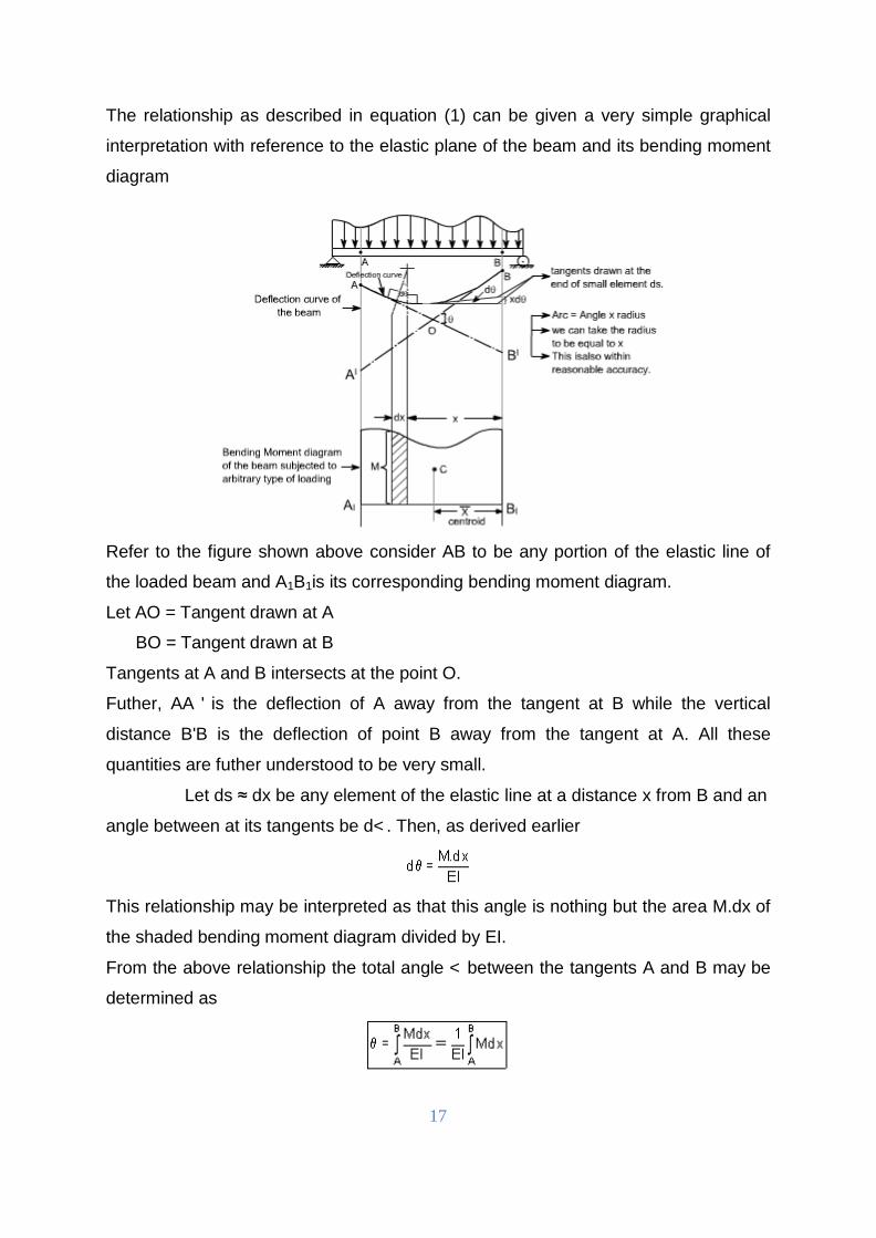
The relationship as described in equation (1) can be given a very simple graphical

interpretation with reference to the elastic plane of the beam and its bending moment

diagram

Refer to the figure shown above consider AB to be any portion of the elastic line of

the loaded beam and A1B1is its corresponding bending moment diagram.

Let AO = Tangent drawn at A

BO = Tangent drawn at B

Tangents at A and B intersects at the point O.

Futher, AA ' is the deflection of A away from the tangent at B while the vertical

distance B'B is the deflection of point B away from the tangent at A. All these

quantities are futher understood to be very small.

Let ds ≈ dx be any element of the elastic line at a distance x from B and an

angle between at its tangents be d< . Then, as derived earlier

This relationship may be interpreted as that this angle is nothing but the area M.dx of

the shaded bending moment diagram divided by EI.

From the above relationship the total angle < between the tangents A and B may be

determined as

18

Since this integral represents the total area of the bending moment diagram, hence

we may conclude this result in the following theorem

Theorem I:

Now let us consider the deflection of point B relative to tangent at A, this is

nothing but the vertical distance BB'. It may be note from the bending diagram that

bending of the element ds contributes to this deflection by an amount equal to x

d< < [each of this intercept may be considered as the arc of a circle of radius x

subtended by the angle < ]

Hence the total distance B'B becomes

The limits from A to B have been taken because A and B are the two points on the

elastic curve, under consideration]. Let us substitute the value of d< = M dx / EI as

derived earlier

diagram]

[ This is infact the moment of area of the bending moment

Since M dx is the area of the shaded strip of the bending moment diagram

and x is its distance from B, we therefore conclude that right hand side of the above

equation represents first moment area with respect to B of the total bending moment

area between A and B divided by EI.

Therefore,we are in a position to state the above conclusion in the form of theorem

as follows:

Theorem II:

Deflection of point ‘B' relative to point A

Futher, the first moment of area, according to the definition of centroid may be

written as , where is equal to distance of centroid and a is the total area of

bending moment

Thus,

19

Therefore,the first moment of area may be obtained simply as a product of the total

area of the B.M diagram betweenthe points A and B multiplied by the distance to

its centroid C.

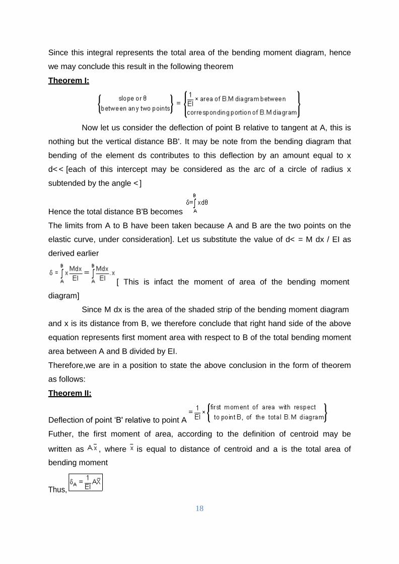
If there exists an inflection point or point of contreflexure for the elastic line of the

loaded beam between the points A and B, as shown below,

Then, adequate precaution must be exercised in using the above theorem. In such a

case B. M diagram gets divide into two portions +ve and –ve portions with centroids

C1and C2. Then to find an angle < between the tangentsat the points A and B

Illustrative Examples: Let us study few illustrative examples, pertaining to the use

of these theorems

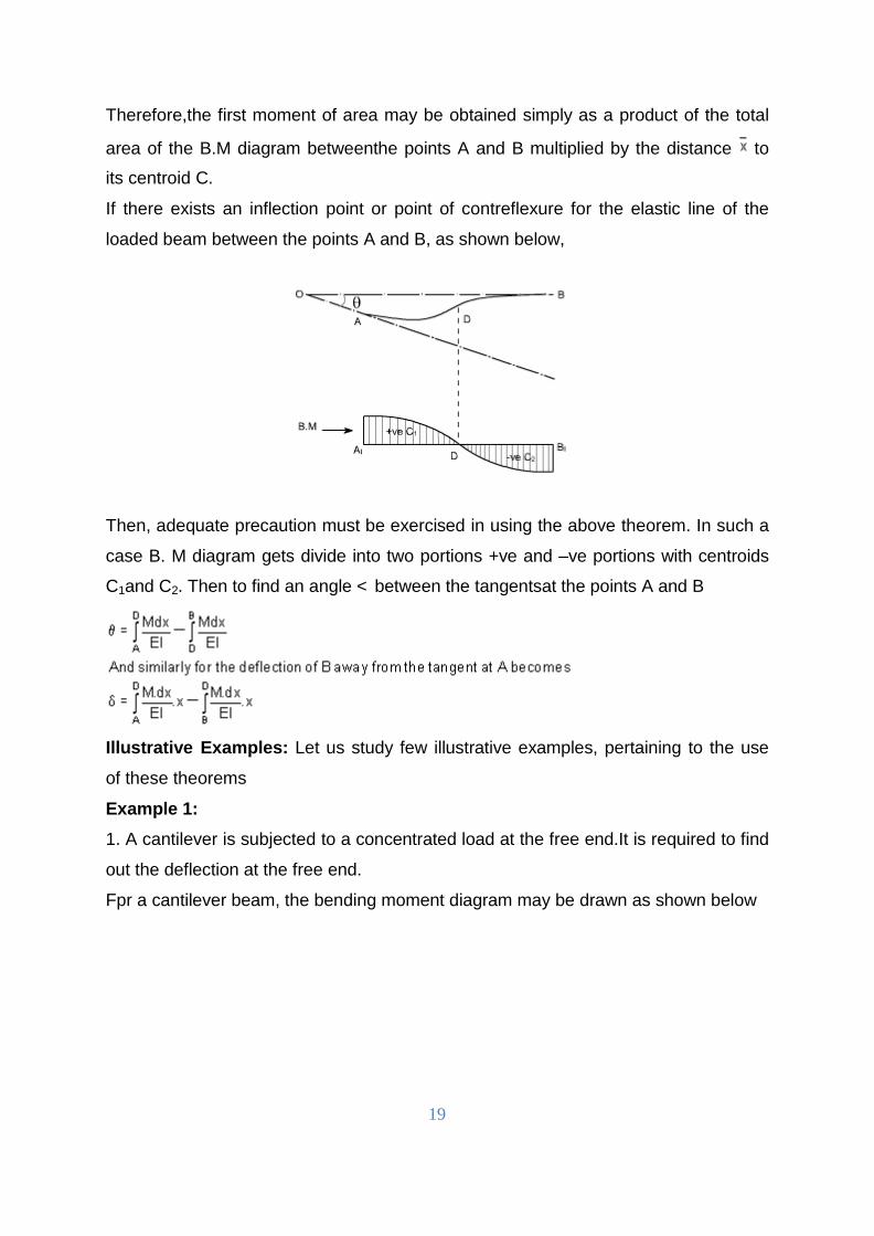
Example 1:

1. A cantilever is subjected to a concentrated load at the free end.It is required to find

out the deflection at the free end.

Fpr a cantilever beam, the bending moment diagram may be drawn as shown below

20

Let us workout this problem from the zero slope condition and apply the first area -

moment theorem

The deflection at A (relative to B) may be obtained by applying the second area -

moment theorem

NOTE: In this case the point B is at zero slope.

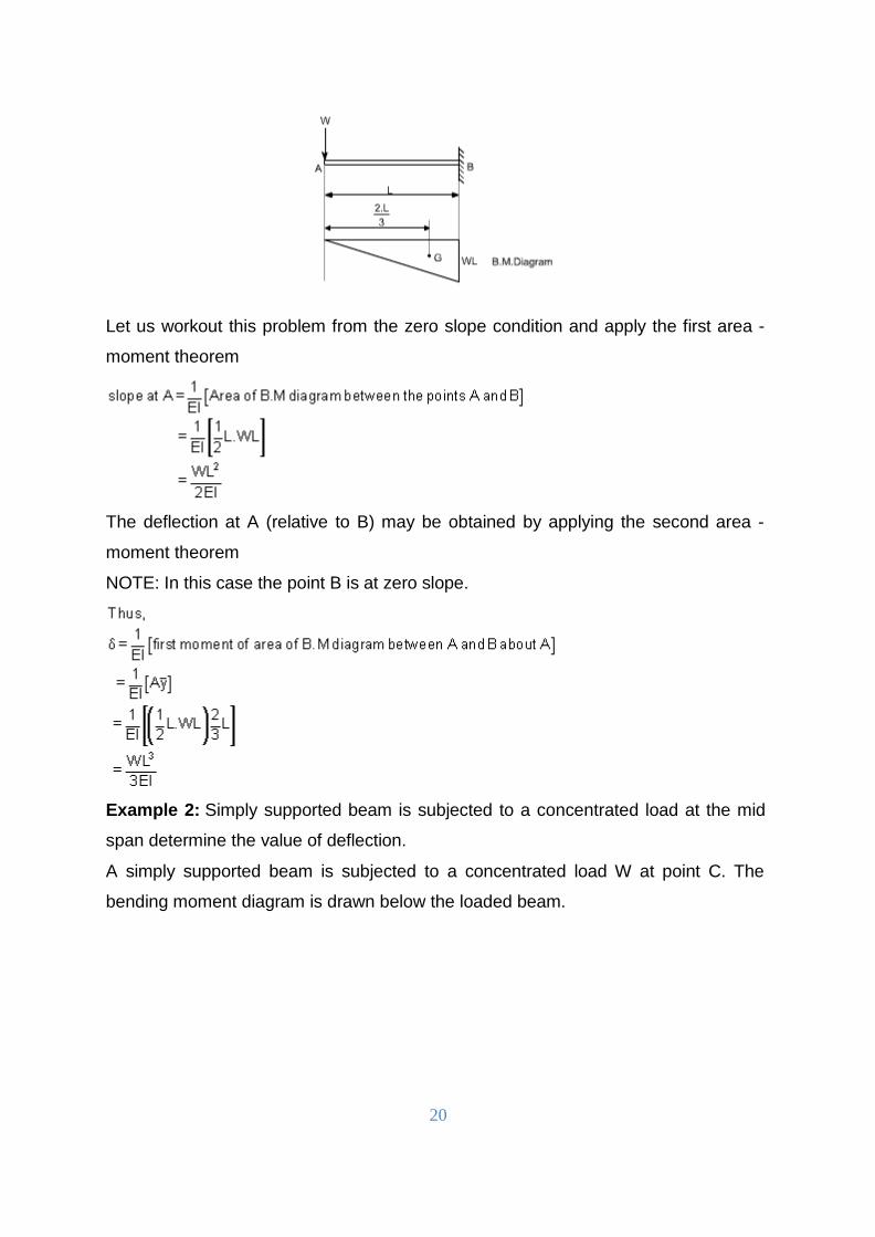
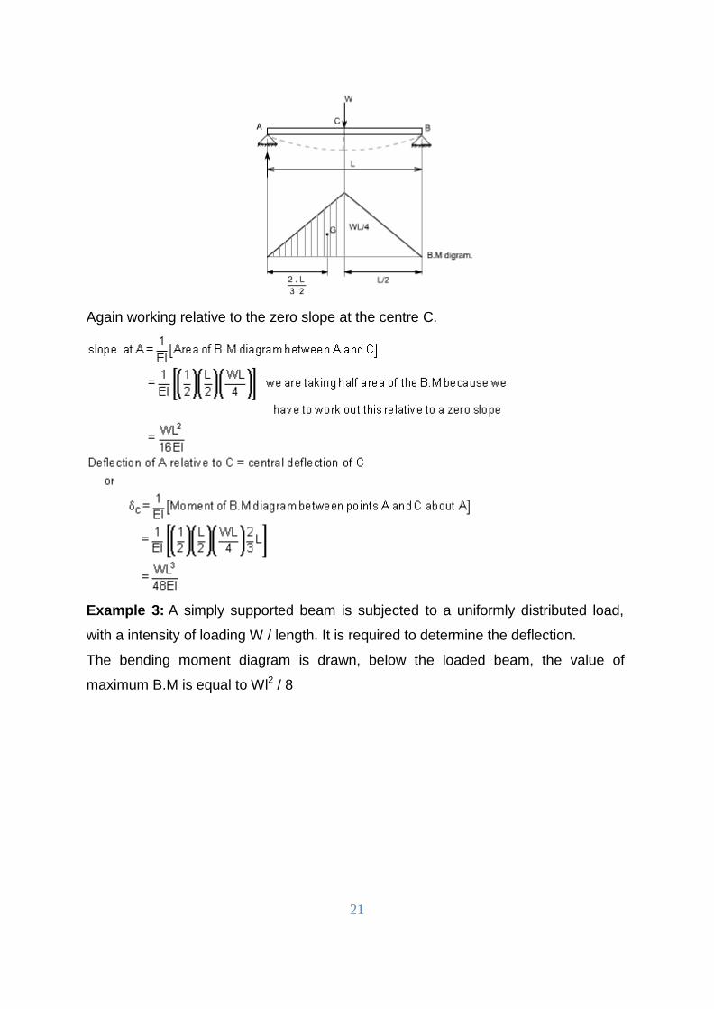
Example 2: Simply supported beam is subjected to a concentrated load at the mid

span determine the value of deflection.

A simply supported beam is subjected to a concentrated load W at point C. The

bending moment diagram is drawn below the loaded beam.

21

Again working relative to the zero slope at the centre C.

Example 3: A simply supported beam is subjected to a uniformly distributed load,

with a intensity of loading W / length. It is required to determine the deflection.

The bending moment diagram is drawn, below the loaded beam, the value of

maximum B.M is equal to Wl2 / 8

22

So by area moment method,

Macaulay's Methods

If the loading conditions change along the span of beam, there is

corresponding change in moment equation. This requires that a separate moment

equation be written between each change of load point and that two integration be

made for each such moment equation. Evaluation of the constants introduced by

each integration can become very involved. Fortunately, these complications can be

avoided by writing single moment equation in such a way that it becomes continuous

for entire length of the beam in spite of the discontinuity of loading.

23

Note : In Macaulay's method some author's take the help of unit function

approximation (i.e. Laplace transform) in order to illustrate this method, however

both are essentially the same.

For example consider the beam shown in fig below:

Let us write the general moment equation using the definition M = ( ∑ M )L, Which

means that we consider the effects of loads lying on the left of an exploratory

section. The moment equations for the portions AB,BC and CD are written as follows

It may be observed that the equation for MCD will also be valid for both MAB and

MBC provided that the terms ( x - 2 ) and ( x - 3 )2are neglected for values of x less

than 2 m and 3 m, respectively. In other words, the terms ( x - 2 ) and ( x - 3 )2 are

nonexistent for values of x for which the terms in parentheses are negative.

As an clear indication of these restrictions,one may use a nomenclature in which the

usual form of parentheses is replaced by pointed brackets, namely, ‹ ›. With this

change in nomenclature, we obtain a single moment equation

24

Which is valid for the entire beam if we postulate that the terms between the pointed

brackets do not exists for negative values; otherwise the term is to be treated like

any ordinary expression.

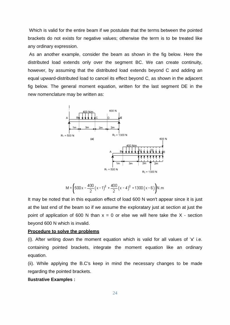
As an another example, consider the beam as shown in the fig below. Here the

distributed load extends only over the segment BC. We can create continuity,

however, by assuming that the distributed load extends beyond C and adding an

equal upward-distributed load to cancel its effect beyond C, as shown in the adjacent

fig below. The general moment equation, written for the last segment DE in the

new nomenclature may be written as:

It may be noted that in this equation effect of load 600 N won't appear since it is just

at the last end of the beam so if we assume the exploratary just at section at just the

point of application of 600 N than x = 0 or else we will here take the X - section

beyond 600 N which is invalid.

Procedure to solve the problems

(i). After writing down the moment equation which is valid for all values of ‘x' i.e.

containing pointed brackets, integrate the moment equation like an ordinary

equation.

(ii). While applying the B.C's keep in mind the necessary changes to be made

regarding the pointed brackets.

llustrative Examples :

25

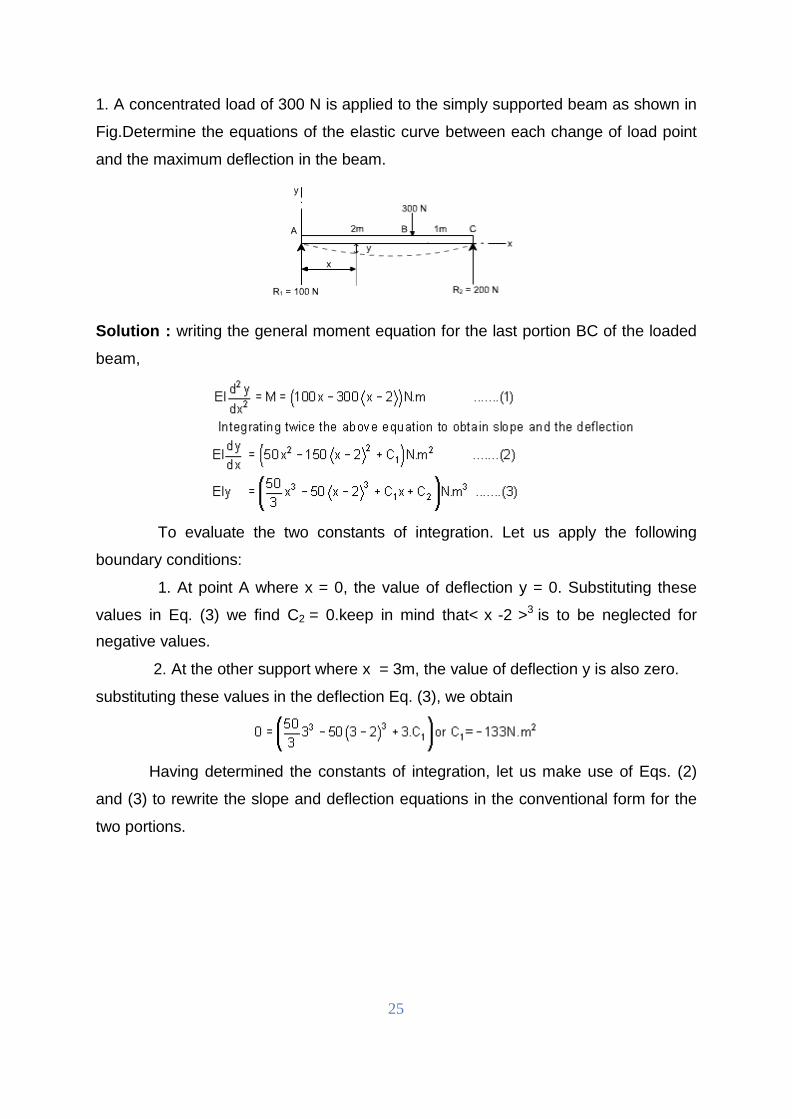
1. A concentrated load of 300 N is applied to the simply supported beam as shown in

Fig.Determine the equations of the elastic curve between each change of load point

and the maximum deflection in the beam.

Solution : writing the general moment equation for the last portion BC of the loaded

beam,

To evaluate the two constants of integration. Let us apply the following

boundary conditions:

1. At point A where x = 0, the value of deflection y = 0. Substituting these

values in Eq. (3) we find C2 = 0.keep in mind that< x -2 >3 is to be neglected for

negative values.

2. At the other support where x = 3m, the value of deflection y is also zero.

substituting these values in the deflection Eq. (3), we obtain

Having determined the constants of integration, let us make use of Eqs. (2)

and (3) to rewrite the slope and deflection equations in the conventional form for the

two portions.

26

Continuing the solution, we assume that the maximum deflection will occur in the

segment AB. Its location may be found by differentiating Eq. (5) with respect to x and

setting the derivative to be equal to zero, or, what amounts to the same thing, setting

the slope equation (4) equal to zero and solving for the point of zero slope.

We obtain

50 x2– 133 = 0 or x = 1.63 m (It may be kept in mind that if the solution of the

equation does not yield a value < 2 m then we have to try the other equations which

are valid for segment BC)

Since this value of x is valid for segment AB, our assumption that the maximum

deflection occurs in this region is correct. Hence, to determine the maximum

deflection, we substitute x = 1.63 m in Eq (5), which yields

The negative value obtained indicates that the deflection y is downward from the x

axis.quite usually only the magnitude of the deflection, without regard to sign, is

desired; this is denoted by < , the use of y may be reserved to indicate a directed

value of deflection.

if E = 30 Gpa and I = 1.9 x 106 mm4 = 1.9 x 10 -6 m4 , Eq. (h) becomes

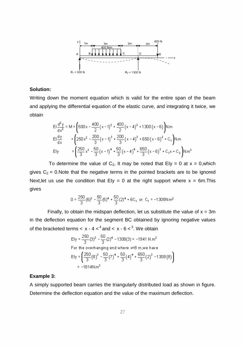
Example 2:

Then

It is required to determine the value of EIy at the position midway between the

supports and at the overhanging end for the beam shown in figure below.

27

Solution:

Writing down the moment equation which is valid for the entire span of the beam

and applying the differential equation of the elastic curve, and integrating it twice, we

obtain

To determine the value of C2, It may be noted that EIy = 0 at x = 0,which

gives C2 = 0.Note that the negative terms in the pointed brackets are to be ignored

Next,let us use the condition that EIy = 0 at the right support where x = 6m.This

gives

Finally, to obtain the midspan deflection, let us substitute the value of x = 3m

in the deflection equation for the segment BC obtained by ignoring negative values

of the bracketed terms < x - 4 < 4 and < x - 6 < 3. We obtain

Example 3:

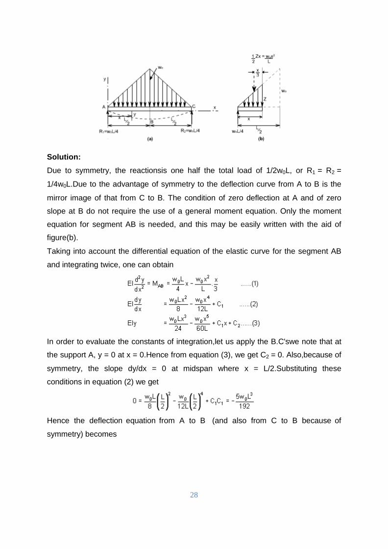
A simply supported beam carries the triangularly distributed load as shown in figure.

Determine the deflection equation and the value of the maximum deflection.

28

Solution:

Due to symmetry, the reactionsis one half the total load of 1/2w0L, or R1 = R2 =

1/4w0L.Due to the advantage of symmetry to the deflection curve from A to B is the

mirror image of that from C to B. The condition of zero deflection at A and of zero

slope at B do not require the use of a general moment equation. Only the moment

equation for segment AB is needed, and this may be easily written with the aid of

figure(b).

Taking into account the differential equation of the elastic curve for the segment AB

and integrating twice, one can obtain

In order to evaluate the constants of integration,let us apply the B.C'swe note that at

the support A, y = 0 at x = 0.Hence from equation (3), we get C2 = 0. Also,because of

symmetry, the slope dy/dx = 0 at midspan where x = L/2.Substituting these

conditions in equation (2) we get

Hence the deflection equation from A to B (and also from C to B because of

symmetry) becomes

29

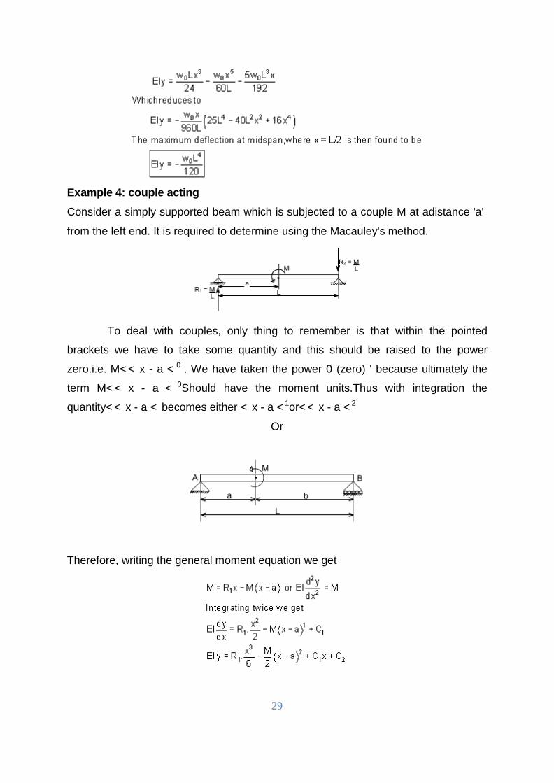
Example 4: couple acting

Consider a simply supported beam which is subjected to a couple M at adistance 'a'

from the left end. It is required to determine using the Macauley's method.

To deal with couples, only thing to remember is that within the pointed

brackets we have to take some quantity and this should be raised to the power

zero.i.e. M< < x - a < 0 . We have taken the power 0 (zero) ' because ultimately the

term M< < x - a < 0Should have the moment units.Thus with integration the

quantity< < x - a < becomes either < x - a < 1or< < x - a < 2

Or

Therefore, writing the general moment equation we get

30

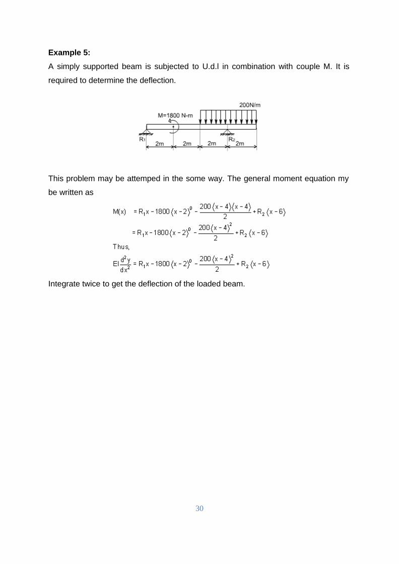
Example 5:

A simply supported beam is subjected to U.d.l in combination with couple M. It is

required to determine the deflection.

This problem may be attemped in the some way. The general moment equation my

be written as

Integrate twice to get the deflection of the loaded beam.

31