Mechanics of Materials 74 (2014) 67–75

Contents lists available at ScienceDirect

Mechanics of Materials

journal homepage: www.elsevier .com/locate /mechmat

Mixed-variational formulation for phononic band-structurecalculation of arbitrary unit cells

http://dx.doi.org/10.1016/j.mechmat.2014.03.0020167-6636/� 2014 Elsevier Ltd. All rights reserved.

⇑ Corresponding author. Tel.: +1 3125673756.E-mail address: asriva13@iit.edu (A. Srivastava).

Ankit Srivastava a,⇑, Sia Nemat-Nasser b

a Department of Mechanical, Materials, and Aerospace Engineering, Illinois Institute of Technology, Chicago, IL 60616, USAb Department of Mechanical and Aerospace Engineering, University of California, La Jolla, San Diego, CA 92093-0416, USA

a r t i c l e i n f o

Article history:Received 27 February 2014Received in revised form 2 March 2014Available online 3 April 2014

Keywords:PhononicsVariational principlesBandstructureBloch wave

a b s t r a c t

This paper presents phononic band-structure calculation results obtained using a mixedvariational formulation for 1-, and 2-dimensional unit cells. The formulation itself is pre-sented in a form which is equally applicable to 3-dimensiomal cases. It has been estab-lished that the mixed-variational formulation presented in this paper shows fasterconvergence with considerably greater accuracy than variational principles based purelyon the displacement field, especially for problems involving unit cells with discontinuousconstituent properties. However, the application of this formulation has been limited tofairly simple unit cells. In this paper we have extended the scope of the formulation byemploying numerical integration techniques making it applicable for the evaluation ofthe phononic band-structure of unit cells displaying arbitrary complexity in their Bravaisstructure and in the shape, size, number, and anisotropicity of their micro-constituents.The approach is demonstrated through specific examples.

� 2014 Elsevier Ltd. All rights reserved.

1. Introduction

There has been a recent surge of research effort towardsachieving exotic dynamic response through novel micro-structural design of composites. Within mechanics andelastodynamics these responses can be categorized intwo broad areas: phononics and metamaterials. Phononicsis the study of stress wave propagation in periodic elasticcomposites, whereas, metamaterials builds upon the areaof phononics with dynamic homogenization schemes andseeks to create periodic composites with overall dynamicproperties that are not shared by common materials. Therequired first step to attain this is to evaluate the phononicband-structure of periodic composites.

The phononic band-structure (Martinezsala et al., 1995)results from the periodic modulation of stress waves, and

as such has deep similarities with areas like electronicband theory (Bloch, 1928) and photonics (Ho et al.,1990). Such periodic modulations provide for very richwave-physics and the potential for novel applications(Cervera et al., 2001; Yang et al., 2002; Khelif et al., 2003;Reed et al., 2003; Yang et al., 2004; Gorishnyy et al.,2005; Mohammadi et al., 2008; Sukhovich et al., 2008;Lin et al., 2009). These applications depend upon the abilityof calculating the required phononic band-structure. Inaddition to the ability of calculating phononic band-struc-tures, certain research areas such as phononic band-struc-ture optimization (Sigmund and Jensen, 2003; Rupp et al.,2007; Bilal and Hussein, 2011; Diaz et al., 2005; Halkjæret al., 2006) and inverse problems in dynamic homogeniza-tion, also demand that the band-structure calculating algo-rithm possess speed, efficiency, accuracy, and versatility.There exist several techniques by which band-structuresof photonic and phononic composites can be computed.These include the plane wave expansion (PWE) method(Ho et al., 1990; Leung and Liu, 1990; Zhang and

68 A. Srivastava, S. Nemat-Nasser / Mechanics of Materials 74 (2014) 67–75

Satpathy, 1990), the multiple scattering method (Kafesakiand Economou, 1999), the finite difference time domainmethod (Chan et al., 1995), the finite element method(White et al., 1989), variational methods (Goffaux andSánchez-Dehesa, 2003) and more (see Hussein, 2009).

In this paper we elaborate upon a mixed variational for-mulation for phononic band-structure calculations whichis based upon varying both the displacement and the stressfields (Nemat-Nasser, 1972; Nemat-Nasser et al., 1975;Minagawa and Nemat-Nasser, 1976; Nemat-Nasser et al.,2011). Since it is based on a variational principle, any setof approximating functions can be used for calculations,e.g., plane-waves Fourier series or finite elements(Minagawa et al., 1981). The mixe formulation yields veryaccurate results and the rate of convergence of the corre-sponding approximating series solution is greater than thatof the Rayleigh quotient with displacement-based approx-imating functions (Babuska and Osborn, 1978). Althoughthe mixed-formulation shows a fast convergence, it hasnot yet been used to evaluate the band-structures of com-plex 2-, and 3-dimensional unit cells. In this paper weextend the scope of the formulation by employing numer-ical integrations and describe clearly how it can be appliedto 1-, 2-, and 3-dimensional unit cells of arbitrary complex-ity in their Bravais structure and in the shape, size, num-ber, and anisotropicity of their micro-constituents. Wepresent 1-, and 2-dimensional test cases which verify theresults of the formulation with published results in litera-ture (exact solution for 1-dimensional and plane waveapproximation for 2-dimensional). For the 2-phase 2-dimensional case we note that acceptable convergenceover the first 18 phononic branches is achieved when thedisplacement and stress fields are approximated by 121Fourier terms each.

2. Statement of the problem

In the following treatment repeated Latin indices meansummation, whereas, repeated Greek indices do not. Con-sider the problem of elastic wave propagation in a general3-dimensional periodic composite. The unit cell of the peri-odic composite is denoted by X and is characterized by 3base vectors hi, i ¼ 1;2;3. Any point within the unit cellcan be uniquely specified by the vector x ¼ Hih

i where0 6 Hi 6 1; i ¼ 1;2;3. The same point can also be specifiedin the orthogonal basis as x ¼ xiei. The reciprocal base vec-tors of the unit cell are given by,

q1 ¼ 2p h2 � h3

h1 � ðh2 � h3Þ; q2 ¼ 2p h3 � h1

h2 � ðh3 � h1Þ; q3

¼ 2p h1 � h2

h3 � ðh1 � h2Þð1Þ

such that qi � hj ¼ 2pdij, where the denominators of theabove vectors are the volume of the unit cell. Fig. 1 is theschematic of a 2-dimensional unit cell, indicating the unitcell basis vectors, the reciprocal basis vectors and theorthogonal basis vectors.

The wave vector for a Bloch-wave traveling in the com-posite are given as k ¼ Qiqi where 0 6 Q i 6 1, i ¼ 1;2;3.

The composite is characterized by a spatially varying stiff-ness tensor, CjkmnðxÞ, and density, qðxÞ, which satisfy thefollowing periodicity conditions:

Cjkmnðxþ nihiÞ ¼ CjkmnðxÞ; qðxþ nih

iÞ ¼ qðxÞ; ð2Þ

where niði ¼ 1;2;3Þ are integers.

2.1. Field equations and boundary conditions

For harmonic elastodynamic problems the equations ofmotion and kinematic relations at any point x in X aregiven by

rjk;k ¼ �kquj; ejk ¼12ðuj;k þ uk;jÞ; ð3Þ

where k ¼ x2, and re�ixt , ee�ixt , and ue�ixt are the spaceand time dependent stress tensor, strain tensor, and dis-placement vector, respectively. The stress tensor is relatedto the strain tensor through the elasticity tensor,rjk ¼ Cjkmnemn. The traction and displacement at any pointin the composite are related to the corresponding tractionand displacement at another point, separated from the firstby a unit cell, through Bloch relations. These relationsserve as the homogeneous boundary conditions on @X. Ifthe Bloch wave vector is k then these boundary conditionsare given by,

ujðxþ hiÞ ¼ ujðxÞeik�hi; tjðxþ hiÞ ¼ �tjðxÞeik�hi

; x 2 @X;ð4Þ

where tj ¼ rjkmk are the components of the traction vectorand m is the exterior unit normal vector on @X.

2.2. Mixed-variational formulation

It has been shown (Nemat-Nasser et al., 1975;Minagawa and Nemat-Nasser, 1976) that the solution to(3) that satisfies the boundary conditions, (4), renders thefollowing functional stationary:

kN ¼hrjk;uj;ki þ huj;k;rjki þ hDjkmnrjk;rmni

hquj;uji; ð5Þ

where D is the compliance tensor and the inner product isgiven by,

hu;vi ¼Z

Xuv�dX; ð6Þ

where v� is the complex conjugate of v.

2.3. Approximation with periodic test functions

Now we approximate the stress and displacement fieldswith the following test functions:

�uj ¼Xa;b;c

Uabcj f abcðxÞ; �rjk ¼

Xa;b;c

Sabcjk f abcðxÞ; ð7Þ

where the test functions satisfy the boundary conditions,(4), and are orthogonal in the sense that hf abc; f hgni is pro-portional to dahdbgdcn, d being the Kronecker delta. Substi-tuting from (7) to (5) and setting the derivative of kN

with respect to the unknown coefficients, (Uabcj ; Sabc

jk ), equal

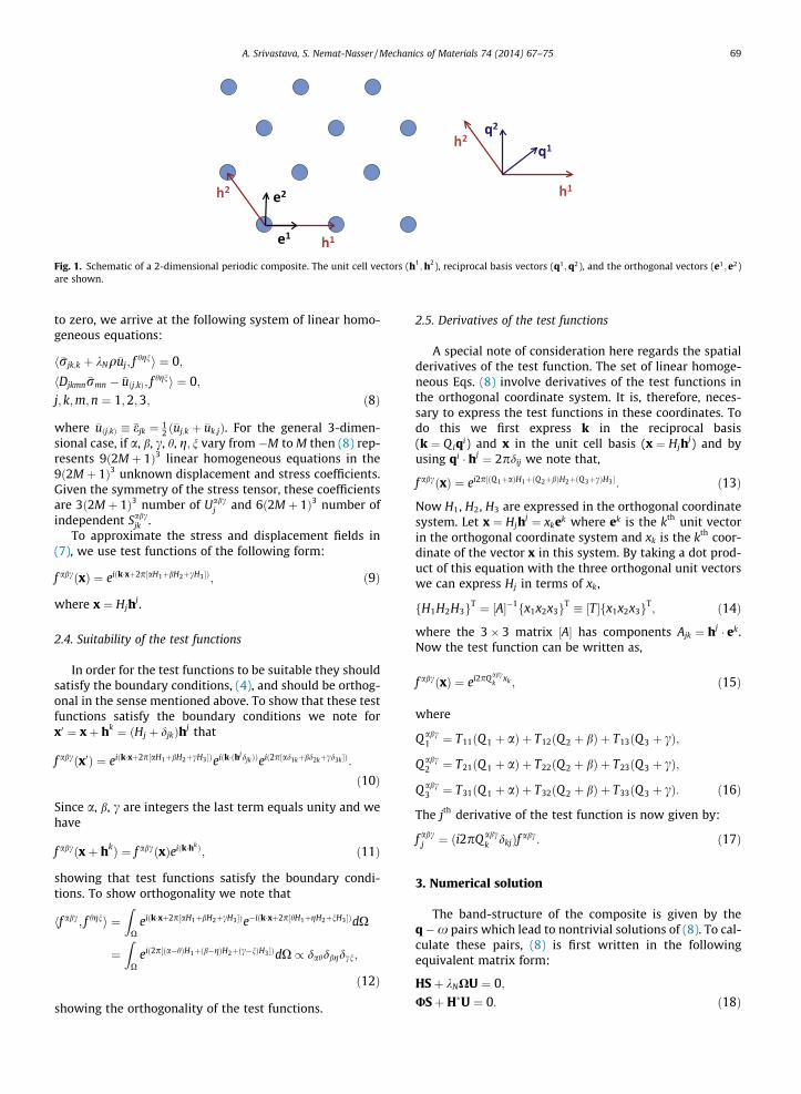
Fig. 1. Schematic of a 2-dimensional periodic composite. The unit cell vectors (h1;h2), reciprocal basis vectors (q1;q2), and the orthogonal vectors (e1; e2)

are shown.

A. Srivastava, S. Nemat-Nasser / Mechanics of Materials 74 (2014) 67–75 69

to zero, we arrive at the following system of linear homo-geneous equations:

h�rjk;k þ kNq�uj; f hgni ¼ 0;

hDjkmn �rmn � �uðj;kÞ; f hgni ¼ 0;j; k;m;n ¼ 1;2;3; ð8Þ

where �uðj;kÞ � �ejk ¼ 12 ð�uj;k þ �uk;jÞ. For the general 3-dimen-

sional case, if a, b, c, h, g; n vary from �M to M then (8) rep-resents 9ð2M þ 1Þ3 linear homogeneous equations in the9ð2M þ 1Þ3 unknown displacement and stress coefficients.Given the symmetry of the stress tensor, these coefficientsare 3ð2M þ 1Þ3 number of Uabc

j and 6ð2M þ 1Þ3 number ofindependent Sabc

jk .To approximate the stress and displacement fields in

(7), we use test functions of the following form:

f abcðxÞ ¼ eiðk�xþ2p½aH1þbH2þcH3 �Þ; ð9Þ

where x ¼ Hjhj.

2.4. Suitability of the test functions

In order for the test functions to be suitable they shouldsatisfy the boundary conditions, (4), and should be orthog-onal in the sense mentioned above. To show that these testfunctions satisfy the boundary conditions we note forx0 ¼ xþ hk ¼ ðHj þ djkÞhj that

f abcðx0Þ ¼ eiðk�xþ2p½aH1þbH2þcH3 �Þeiðk�ðhjdjkÞÞeið2p½ad1kþbd2kþcd3k �Þ:

ð10Þ

Since a, b, c are integers the last term equals unity and wehave

f abcðxþ hkÞ ¼ f abcðxÞeiðk�hkÞ; ð11Þ

showing that test functions satisfy the boundary condi-tions. To show orthogonality we note that

hf abc; f hgni ¼Z

Xeiðk�xþ2p½aH1þbH2þcH3 �Þe�iðk�xþ2p½hH1þgH2þnH3 �ÞdX

¼Z

Xeið2p½ða�hÞH1þðb�gÞH2þðc�nÞH3 �ÞdX / dahdbgdcn;

ð12Þ

showing the orthogonality of the test functions.

2.5. Derivatives of the test functions

A special note of consideration here regards the spatialderivatives of the test function. The set of linear homoge-neous Eqs. (8) involve derivatives of the test functions inthe orthogonal coordinate system. It is, therefore, neces-sary to express the test functions in these coordinates. Todo this we first express k in the reciprocal basis(k ¼ Q iqi) and x in the unit cell basis (x ¼ Hjh

j) and byusing qi � hj ¼ 2pdij we note that,

f abcðxÞ ¼ ei2p½ðQ1þaÞH1þðQ2þbÞH2þðQ3þcÞH3 �: ð13Þ

Now H1, H2, H3 are expressed in the orthogonal coordinatesystem. Let x ¼ Hjh

j ¼ xkek where ek is the kth unit vectorin the orthogonal coordinate system and xk is the kth coor-dinate of the vector x in this system. By taking a dot prod-uct of this equation with the three orthogonal unit vectorswe can express Hj in terms of xk,

fH1H2H3gT ¼ ½A��1fx1x2x3gT � ½T�fx1x2x3gT; ð14Þ

where the 3� 3 matrix ½A� has components Ajk ¼ hj � ek.Now the test function can be written as,

f abcðxÞ ¼ ei2pQabck

xk ; ð15Þ

where

Qabc1 ¼ T11ðQ 1 þ aÞ þ T12ðQ 2 þ bÞ þ T13ðQ 3 þ cÞ;

Qabc2 ¼ T21ðQ 1 þ aÞ þ T22ðQ 2 þ bÞ þ T23ðQ 3 þ cÞ;

Qabc3 ¼ T31ðQ 1 þ aÞ þ T32ðQ 2 þ bÞ þ T33ðQ 3 þ cÞ: ð16Þ

The jth derivative of the test function is now given by:

f abc;j ¼ ði2pQabc

k dkjÞf abc: ð17Þ

3. Numerical solution

The band-structure of the composite is given by theq�x pairs which lead to nontrivial solutions of (8). To cal-culate these pairs, (8) is first written in the followingequivalent matrix form:

HSþ kNXU ¼ 0;USþH�U ¼ 0: ð18Þ

70 A. Srivastava, S. Nemat-Nasser / Mechanics of Materials 74 (2014) 67–75

Column vectors S;U contain the unknown coefficients ofthe periodic expansions of stress and displacement, respec-tively. Matrices H, X, U, H� contain the integrals of the var-ious functions appearing in (8). Their sizes depend uponwhether the problem under consideration is 1-, 2-, or 3-dimensional. These matrices would be described moreclearly in the subsequent sections in which numericalexamples are shown. The above system of equations canbe recast into the following traditional eigenvalueproblem:

ðHU�1H�Þ�1XU ¼ 1

kNU; ð19Þ

whose eigenvalue solutions represent the frequencies(xN ¼

ffiffiffiffiffikNp

) associated with the wave-vector under consid-eration (q). The eigenvectors of the above equation areused to calculate the displacement modeshapes from (7).The relation S ¼ �U�1H�U is used to evaluate the stresseigenvector which is subsequently used to calculate thestress modeshape from (7).

The integrals occurring in (18) are numerically calcu-lated over X. This is a diversion from the earlier results(Nemat-Nasser et al., 1975; Minagawa and Nemat-Nasser, 1976) where the closed form solutions of the inte-grals were used. By numerically evaluating the integralswe have extended the scope of the method to include arbi-trary inclusions and all possible Bravais lattices in 1-, 2-,and 3-dimensions. Numerical integration is achieved bydividing the domain X into P subdomains Xi,i ¼ 1;2; . . . ; P. The volume integral of any function FðxÞ isthen approximated as,

ZX

FðxÞdX ¼XP

i

FiV i; ð20Þ

where Fi is the value of the function FðxÞ evaluated at thecentroid of Xi and Vi is the volume of Xi. For meshing in2-, and 3-D we have used a freely available Finite Elementsoftware Geuzaine and Remacle, 2009 which automaticallydiscretizes the domain in triangular (for 2-D) and tetrahe-dral (in 3-D) elements and provides the nodal position andelemental connectivity matrices. MATLAB (or Python) rou-tines are then used to calculate the volumes and centroidsof these subdomains and the required integrals over X.

4. Application to 1-D periodic composites

There is only one possible Bravais lattice in 1-dimensionwith a unit cell vector whose length equals the length ofthe unit cell itself. Without any loss of generality we takethe direction of this vector to be the same as e1. If thelength of the unit cell is a, then we have h1 ¼ ae1. The reci-procal vector is given by q1 ¼ ð2p=aÞe1. The wave-vector ofa Bloch wave traveling in this composite is specified ask ¼ Q 1q1. To completely characterize the band-structureof the unit cell it is sufficient to evaluate the dispersionrelation in the irreducible Brillouin zone (�:5 6 Q 1 6 :5).

For plane longitudinal wave propagating in the e1 direc-tion the only displacement component of interest is u1 andthe only relevant stress component is r11 (for plane shearwaves traveling in e1 direction the quantities of interest

are u2 and r12, and for the anti-plane shear waves, theyare u3 and r13, respectively). The equation of motion andthe constitutive relation are,

r11;1 ¼ �kqðx1Þu1; r11 ¼ Eðx1Þu1;1; ð21Þ

where Eðx1Þ is the spatially varying Young’s modulus.These are approximated by 1-D periodic functions,

�u1 ¼XM

a¼�M

Ua1eiðk�xþ2paH1Þ; �r11 ¼

XM

a¼�M

Sa11eiðk�xþ2paH1Þ; ð22Þ

which can be further simplified to,

�u1 ¼XM

a¼�M

Ua1ei2pðQ1þaÞx1=a; �r11 ¼

XM

a¼�M

Sa11ei2pðQ1þaÞx1=a:

ð23Þ

Now the system of equations denoting the eigenvalueproblem are written as:

h�r11;1 þ kNq�u1; f hi ¼ 0;

hD�r11 � �u1;1; f hi ¼ 0; ð24Þ

where M 6 a; h 6 M and D ¼ 1=E. The above are trans-formed to the matrix form of (18) with the following col-umn vectors:

U ¼ fU�M1 . . . U0

1 . . . UM1 g

T;

S ¼ fS�M11 . . . S0

11 . . . SM11g

T: ð25Þ

The associated coefficient matrices have the followingelements:

½H�mn ¼i2pðQ1 þm�M � 1Þ

a

Z a

0ei2pðm�nÞx1=adx1;

½X�mn ¼Z a

0qðx1Þei2pðm�nÞx1=adx1;

½U�mn ¼Z a

0Dðx1Þei2pðm�nÞx1=adx1;

½H��mn ¼�i2pðQ 1 þm�M � 1Þ

a

Z a

0ei2pðm�nÞx1=adx1;

m;n ¼ 1;2; . . . ; ð2M þ 1Þ: ð26Þ

It must be noted that given the periodicity of the expo-nential function, matrices ½H� and ½H�� are diagonal. Nowfor given values of Q 1, the eigenvalue problem can besolved for the frequencies xN .

4.1. 2-Phase layered composite: comparison with Rytovsolution

The problem of wave propagation in 1-dimension lay-ered composite can be solved exactly. For a 2-phase com-posite this solution was first given by Rytov Rytov(1956). Here we show a comparison of the results fromthe mixed-variational formulation with the exact Rytovsolution. Since for the 1-dimensional case the integrals in(26) can be calculated exactly, we have not employednumerical integration via discretization of X.

The composite under consideration is a 2-phase com-posite with X consisting of the following 2 phases:

A. Srivastava, S. Nemat-Nasser / Mechanics of Materials 74 (2014) 67–75 71

1. Phase 1: E ¼ 8 Gpa, q ¼ 1000 kg/m3,thickness = 0.003 m

2. Phase 2: E ¼ 300 Gpa, q ¼ 8000 kg/m3,thickness = 0.001 m

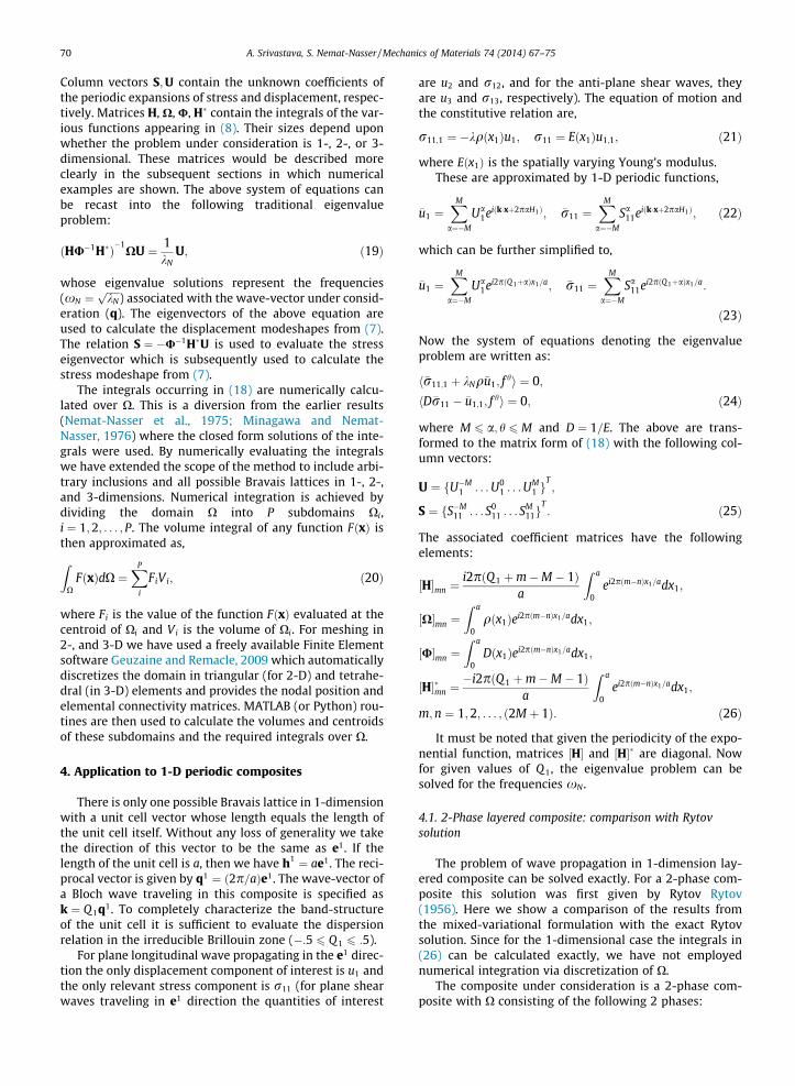
Fig. 2 shows the comparison of the results from themixed-variational formulation with the Rytov solution forthe first four branches of the composite. The results are cal-culated for 0 6 Q 1 6 :5 at a total of 155 points. The mixed-variational results are shown for M ¼ 2;3. At each value ofQ 1 the eigenvalue solution results in 2M þ 1 frequencies.This process is repeated for the 155 values of Q 1 between0 and 0.5. From the results in Fig. 2 it is clear that the firsttwo branches are captured well even with M ¼ 2 whereashigher branches require more terms in the periodic expan-sion for adequate accuracy. Convergence to the exact solu-tion is achieved for all branches as higher number of termsare used in the expansion.

The cpu-time as calculated from the cputime commandin MATLAB gives an average value of 0.11544 s for M ¼ 2computations and 0.15912 s for M ¼ 3 computations. Itmust be stressed that in each case this cpu-time refers tothe time it takes to calculate all 2M þ 1 frequencies forall 155 Q1-points. Fig. 3 shows the average computationtime as given by the cpu-time command for M rangingfrom 1 to 10.

5. Application to 2-D periodic composites

There are five possible Bravais lattices in 2 dimensions.However, they can be specified using two unit cell vectors(h1

;h2). The reciprocal vector are q1;q2. The wave-vectorof a Bloch-wave traveling in this composite is specified ask ¼ Q 1q1 þ Q 2q2. To characterize the band-structure ofthe unit cell we evaluate the dispersion relation alongthe boundaries of the irreducible Brillouin zone(0 6 Q 1 6 :5, Q 2 ¼ 0; Q1 ¼ :5;0 6 Q 2 6 :5; 0 6 Q1 6

Fig. 2. Comparison of the mixed-variational formulation results wit

:5;Q 2 ¼ Q 1). In traditional notation these boundaries arespecified as C� X;X �M;M � C, respectively. Therefore,we would be considering band-structure overC� X �M � C.

For purposes of demonstration and comparison we con-sider the case of plane-strain state in the composite. Therelevant stress components for the plane-strain case arer11, r22, r12 and the relevant displacement componentsare u1;u2. The equations of motion and the constitutiverelation are,

rjk;k ¼ �kqðxÞuj; DjkmnðxÞrmn ¼ uj;k;

j; k;m;n ¼ 1;2; ð27Þ

where D is the compliance tensor. For an isotropic materialin plane strain, D is given by,

Djkmn ¼1

2l12ðdjmdkn þ djndkmÞ �

k2ðlþ kÞ djkdmn

� �;

j; k;m;n ¼ 1;2; ð28Þ

where k;l are the Lame0 constants. The stresses and dis-placements are approximated by the following 2-D peri-odic functions:

�uj ¼XM

a;b¼�M

Uabj ei2pQab

lxl ;

�rjk ¼XM

a;b¼�M

Sabjk ei2pQab

lxl ; j; k; l ¼ 1;2; ð29Þ

where

Qab1 ¼ T11ðQ1 þ aÞ þ T21ðQ 2 þ bÞ;

Qab2 ¼ T12ðQ1 þ aÞ þ T22ðQ 2 þ bÞ; ð30Þ

and the square matrix ½T� is the inverse of the matrix ½A�with components ½A�jk ¼ hj � ek.

h Rytov solution. The first 4 branches are shown for M ¼ 2;3.

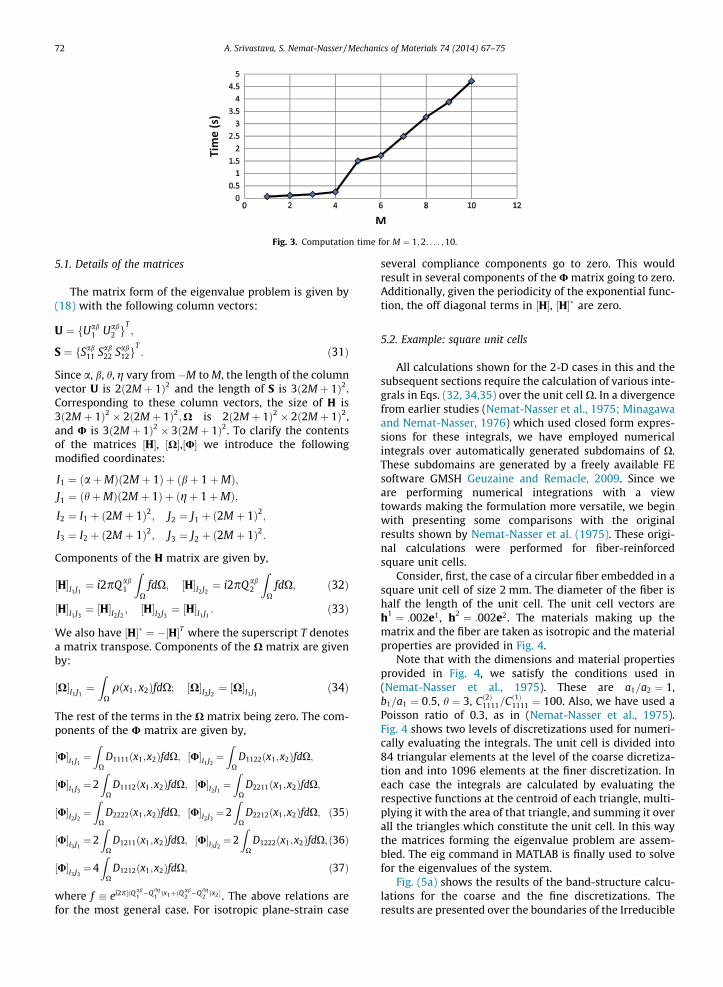
Fig. 3. Computation time for M ¼ 1;2; . . . ;10.

72 A. Srivastava, S. Nemat-Nasser / Mechanics of Materials 74 (2014) 67–75

5.1. Details of the matrices

The matrix form of the eigenvalue problem is given by(18) with the following column vectors:

U ¼ fUab1 Uab

2 gT;

S ¼ fSab11 Sab

22 Sab12g

T: ð31Þ

Since a, b, h, g vary from �M to M, the length of the columnvector U is 2ð2M þ 1Þ2 and the length of S is 3ð2M þ 1Þ2.Corresponding to these column vectors, the size of H is3ð2M þ 1Þ2 � 2ð2M þ 1Þ2;X is 2ð2M þ 1Þ2 � 2ð2M þ 1Þ2,and U is 3ð2M þ 1Þ2 � 3ð2M þ 1Þ2. To clarify the contentsof the matrices ½H�, ½X�,½U� we introduce the followingmodified coordinates:

I1 ¼ ðaþMÞð2M þ 1Þ þ ðbþ 1þMÞ;J1 ¼ ðhþMÞð2M þ 1Þ þ ðgþ 1þMÞ;I2 ¼ I1 þ ð2M þ 1Þ2; J2 ¼ J1 þ ð2M þ 1Þ2;I3 ¼ I2 þ ð2M þ 1Þ2; J3 ¼ J2 þ ð2M þ 1Þ2:

Components of the H matrix are given by,

½H�I1 J1¼ i2pQab

1

ZX

fdX; ½H�I2 J2¼ i2pQab

2

ZX

fdX; ð32Þ

½H�I1 J3¼ ½H�I2 J2

; ½H�I2J3¼ ½H�I1 J1

: ð33Þ

We also have ½H�� ¼ �½H�T where the superscript T denotesa matrix transpose. Components of the X matrix are givenby:

½X�I1 J1¼Z

Xqðx1; x2ÞfdX; ½X�I2J2

¼ ½X�I1 J1ð34Þ

The rest of the terms in the X matrix being zero. The com-ponents of the U matrix are given by,

½U�I1 J1¼Z

XD1111ðx1;x2ÞfdX; ½U�I1 J2

¼Z

XD1122ðx1;x2ÞfdX;

½U�I1 J3¼2

ZX

D1112ðx1;x2ÞfdX; ½U�I2 J1¼Z

XD2211ðx1;x2ÞfdX;

½U�I2 J2¼Z

XD2222ðx1;x2ÞfdX; ½U�I2 J3

¼2Z

XD2212ðx1;x2ÞfdX; ð35Þ

½U�I3 J1¼2

ZX

D1211ðx1;x2ÞfdX; ½U�I3 J2¼2

ZX

D1222ðx1;x2ÞfdX; ð36Þ

½U�I3 J3¼4

ZX

D1212ðx1;x2ÞfdX; ð37Þ

where f � ei2p½ðQab1 �Qhg

1 Þx1þðQab2 �Qhg

2 Þx2 �. The above relations arefor the most general case. For isotropic plane-strain case

several compliance components go to zero. This wouldresult in several components of the U matrix going to zero.Additionally, given the periodicity of the exponential func-tion, the off diagonal terms in ½H�, ½H�� are zero.

5.2. Example: square unit cells

All calculations shown for the 2-D cases in this and thesubsequent sections require the calculation of various inte-grals in Eqs. (32, 34,35) over the unit cell X. In a divergencefrom earlier studies (Nemat-Nasser et al., 1975; Minagawaand Nemat-Nasser, 1976) which used closed form expres-sions for these integrals, we have employed numericalintegrals over automatically generated subdomains of X.These subdomains are generated by a freely available FEsoftware GMSH Geuzaine and Remacle, 2009. Since weare performing numerical integrations with a viewtowards making the formulation more versatile, we beginwith presenting some comparisons with the originalresults shown by Nemat-Nasser et al. (1975). These origi-nal calculations were performed for fiber-reinforcedsquare unit cells.

Consider, first, the case of a circular fiber embedded in asquare unit cell of size 2 mm. The diameter of the fiber ishalf the length of the unit cell. The unit cell vectors areh1 ¼ :002e1, h2 ¼ :002e2. The materials making up thematrix and the fiber are taken as isotropic and the materialproperties are provided in Fig. 4.

Note that with the dimensions and material propertiesprovided in Fig. 4, we satisfy the conditions used in(Nemat-Nasser et al., 1975). These are a1=a2 ¼ 1,b1=a1 ¼ 0:5, h ¼ 3, Cð2Þ1111=Cð1Þ1111 ¼ 100. Also, we have used aPoisson ratio of 0.3, as in (Nemat-Nasser et al., 1975).Fig. 4 shows two levels of discretizations used for numeri-cally evaluating the integrals. The unit cell is divided into84 triangular elements at the level of the coarse dicretiza-tion and into 1096 elements at the finer discretization. Ineach case the integrals are calculated by evaluating therespective functions at the centroid of each triangle, multi-plying it with the area of that triangle, and summing it overall the triangles which constitute the unit cell. In this waythe matrices forming the eigenvalue problem are assem-bled. The eig command in MATLAB is finally used to solvefor the eigenvalues of the system.

Fig. (5a) shows the results of the band-structure calcu-lations for the coarse and the fine discretizations. Theresults are presented over the boundaries of the Irreducible

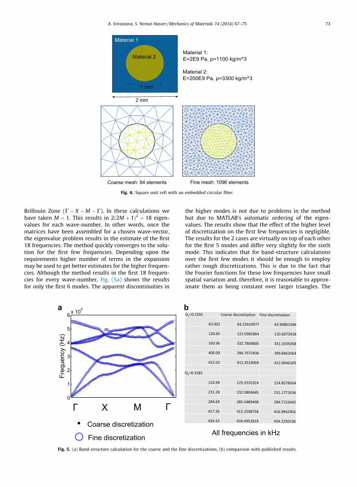
Fig. 4. Square unit cell with an embedded circular fiber.

A. Srivastava, S. Nemat-Nasser / Mechanics of Materials 74 (2014) 67–75 73

Brillouin Zone (C� X �M � C). In these calculations wehave taken M ¼ 1. This results in 2ð2M þ 1Þ2 ¼ 18 eigen-values for each wave-number. In other words, once thematrices have been assembled for a chosen wave-vector,the eigenvalue problem results in the estimate of the first18 frequencies. The method quickly converges to the solu-tion for the first few frequencies. Depending upon therequirements higher number of terms in the expansionmay be used to get better estimates for the higher frequen-cies. Although the method results in the first 18 frequen-cies for every wave-number, Fig. (5a) shows the resultsfor only the first 6 modes. The apparent discontinuities in

a

Fig. 5. (a) Band-structure calculation for the coarse and the fin

the higher modes is not due to problems in the methodbut due to MATLAB’s automatic ordering of the eigen-values. The results show that the effect of the higher levelof discretization on the first few frequencies is negligible.The results for the 2 cases are virtually on top of each otherfor the first 5 modes and differ very slightly for the sixthmode. This indicates that for band-structure calculationsover the first few modes it should be enough to employrather rough discretizations. This is due to the fact thatthe Fourier functions for these low frequencies have smallspatial variation and, therefore, it is reasonable to approx-imate them as being constant over larger triangles. The

b

e discretizations, (b) comparison with published results.

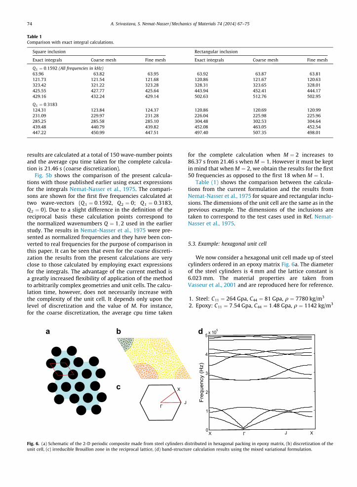
Table 1Comparison with exact integral calculations.

Square inclusion Rectangular inclusion

Exact integrals Coarse mesh Fine mesh Exact integrals Coarse mesh Fine mesh

Q1 ¼ 0:1592 (All frequencies in kHz)63.96 63.82 63.95 63.92 63.87 63.81121.73 121.54 121.68 120.86 121.67 120.63323.42 321.22 323.28 328.31 323.65 328.01425.55 427.77 425.64 443.94 452.41 444.17429.16 432.24 429.14 502.63 512.76 502.95

Q1 ¼ 0:3183124.31 123.84 124.37 120.86 120.69 120.99231.09 229.97 231.28 226.04 225.98 225.96285.25 285.58 285.10 304.48 302.53 304.64439.48 440.79 439.82 452.08 463.05 452.54447.22 450.99 447.51 497.40 507.35 498.01

74 A. Srivastava, S. Nemat-Nasser / Mechanics of Materials 74 (2014) 67–75

results are calculated at a total of 150 wave-number pointsand the average cpu time taken for the complete calcula-tion is 21.46 s (coarse discretization).

Fig. 5b shows the comparison of the present calcula-tions with those published earlier using exact expressionsfor the integrals Nemat-Nasser et al., 1975. The compari-sons are shown for the first five frequencies calculated attwo wave-vectors (Q 1 ¼ 0:1592, Q2 ¼ 0; Q 1 ¼ 0:3183,Q2 ¼ 0). Due to a slight difference in the definition of thereciprocal basis these calculation points correspond tothe normalized wavenumbers Q ¼ 1;2 used in the earlierstudy. The results in Nemat-Nasser et al., 1975 were pre-sented as normalized frequencies and they have been con-verted to real frequencies for the purpose of comparison inthis paper. It can be seen that even for the coarse discreti-zation the results from the present calculations are veryclose to those calculated by employing exact expressionsfor the integrals. The advantage of the current method isa greatly increased flexibility of application of the methodto arbitrarily complex geometries and unit cells. The calcu-lation time, however, does not necessarily increase withthe complexity of the unit cell. It depends only upon thelevel of discretization and the value of M. For instance,for the coarse discretization, the average cpu time taken

a b

c

Fig. 6. (a) Schematic of the 2-D periodic composite made from steel cylinders dunit cell, (c) irreducible Brouillon zone in the reciprocal lattice, (d) band-structu

for the complete calculation when M ¼ 2 increases to86.37 s from 21.46 s when M ¼ 1. However it must be keptin mind that when M ¼ 2, we obtain the results for the first50 frequencies as opposed to the first 18 when M ¼ 1.

Table (1) shows the comparison between the calcula-tions from the current formulation and the results fromNemat-Nasser et al., 1975 for square and rectangular inclu-sions. The dimensions of the unit cell are the same as in theprevious example. The dimensions of the inclusions aretaken to correspond to the test cases used in Ref. Nemat-Nasser et al., 1975.

5.3. Example: hexagonal unit cell

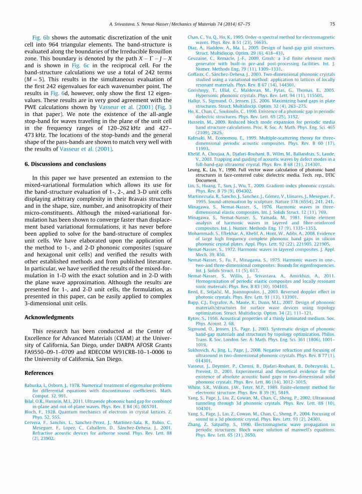
We now consider a hexagonal unit cell made up of steelcylinders ordered in an epoxy matrix Fig. 6a. The diameterof the steel cylinders is 4 mm and the lattice constant is6.023 mm. The material properties are taken fromVasseur et al., 2001 and are reproduced here for reference.

1. Steel: C11 ¼ 264 Gpa, C44 ¼ 81 Gpa, q ¼ 7780 kg/m3

2. Epoxy: C11 ¼ 7:54 Gpa, C44 ¼ 1:48 Gpa, q ¼ 1142 kg/m3

d

istributed in hexagonal packing in epoxy matrix, (b) discretization of there calculation results using the mixed variational formulation.

A. Srivastava, S. Nemat-Nasser / Mechanics of Materials 74 (2014) 67–75 75

Fig. 6b shows the automatic discretization of the unitcell into 964 triangular elements. The band-structure isevaluated along the boundaries of the Irreducible Brouillonzone. This boundary is denoted by the path X � C� J � Xand is shown in Fig. 6c in the reciprocal cell. For theband-structure calculations we use a total of 242 terms(M ¼ 5). This results in the simultaneous evaluation ofthe first 242 eigenvalues for each wavenumber point. Theresults in Fig. 6d, however, only show the first 12 eigen-values. These results are in very good agreement with thePWE calculations shown by Vasseur et al. (2001) (Fig. 3in that paper). We note the existence of the all-anglestop-band for waves traveling in the plane of the unit cellin the frequency ranges of 120–262 kHz and 427–473 kHz. The locations of the stop-bands and the generalshape of the pass-bands are shown to match very well withthe results of Vasseur et al. (2001).

6. Discussions and conclusions

In this paper we have presented an extension to themixed-variational formulation which allows its use forthe band-structure evaluation of 1-, 2-, and 3-D unit cellsdisplaying arbitrary complexity in their Bravais structureand in the shape, size, number, and anisotropicity of theirmicro-constituents. Although the mixed-variational for-mulation has been shown to converge faster than displace-ment based variational formulations, it has never beforebeen applied to solve for the band-structure of complexunit cells. We have elaborated upon the application ofthe method to 1-, and 2-D phononic composites (squareand hexagonal unit cells) and verified the results withother established methods and from published literature.In particular, we have verified the results of the mixed-for-mulation in 1-D with the exact solution and in 2-D withthe plane wave approximation. Although the results arepresented for 1-, and 2-D unit cells, the formulation, aspresented in this paper, can be easily applied to complex3-dimensional unit cells.

Acknowledgments

This research has been conducted at the Center ofExcellence for Advanced Materials (CEAM) at the Univer-sity of California, San Diego, under DARPA AFOSR GrantsFA9550–09-1–0709 and RDECOM W91CRB-10–1-0006 tothe University of California, San Diego.

References

Babuska, I., Osborn, J., 1978. Numerical treatment of eigenvalue problemsfor differential equations with discontinuous coefficients. Math.Comput. 32, 991.

Bilal, O.R., Hussein, M.I., 2011. Ultrawide phononic band gap for combinedin-plane and out-of-plane waves. Phys. Rev. E 84 (6), 065701.

Bloch, F., 1928. Quantum mechanics of electrons in crystal lattices. Z.Phys. 52, 555.

Cervera, F., Sanchis, L., Sanchez-Perez, J., Martinez-Sala, R., Rubio, C.,Meseguer, F., Lopez, C., Caballero, D., Sánchez-Dehesa, J., 2001.Refractive acoustic devices for airborne sound. Phys. Rev. Lett. 88(2), 23902.

Chan, C., Yu, Q., Ho, K., 1995. Order-n spectral method for electromagneticwaves. Phys. Rev. B 51 (23), 16635.

Diaz, A., Haddow, A., Ma, L., 2005. Design of band-gap grid structures.Struct. Multidiscip. Optim. 29 (6), 418–431.

Geuzaine, C., Remacle, J.-F., 2009. Gmsh: a 3-d finite element meshgenerator with built-in pre-and post-processing facilities. Int. J.Numer. Methods Eng. 79 (11), 1309–1331.

Goffaux, C., Sánchez-Dehesa, J., 2003. Two-dimensional phononic crystalsstudied using a variational method: application to lattices of locallyresonant materials. Phys. Rev. B 67 (14), 144301.

Gorishnyy, T., Ullal, C., Maldovan, M., Fytas, G., Thomas, E., 2005.Hypersonic phononic crystals. Phys. Rev. Lett. 94 (11), 115501.

Halkjr, S., Sigmund, O., Jensen, J.S., 2006. Maximizing band gaps in platestructures. Struct. Multidiscip. Optim. 32 (4), 263–275.

Ho, K., Chan, C., Soukoulis, C., 1990. Existence of a photonic gap in periodicdielectric structures. Phys. Rev. Lett. 65 (25), 3152.

Hussein, M., 2009. Reduced bloch mode expansion for periodic mediaband structure calculations. Proc. R. Soc. A: Math. Phys. Eng. Sci. 465(2109), 2825.

Kafesaki, M., Economou, E., 1999. Multiple-scattering theory for three-dimensional periodic acoustic composites. Phys. Rev. B 60 (17),11993.

Khelif, A., Choujaa, A., Djafari-Rouhani, B., Wilm, M., Ballandras, S., Laude,V., 2003. Trapping and guiding of acoustic waves by defect modes in afull-band-gap ultrasonic crystal. Phys. Rev. B 68 (21), 214301.

Leung, K., Liu, Y., 1990. Full vector wave calculation of photonic bandstructures in face-centered cubic dielectric media. Tech. rep., DTICDocument.

Lin, S., Huang, T., Sun, J., Wu, T., 2009. Gradient-index phononic crystals.Phys. Rev. B 79 (9), 094302.

Martinezsala, R., Sancho, J., Sanchez, J., Gómez, V., Llinares, J., Meseguer, F.,1995. Sound-attenuation by sculpture. Nature 378 (6554), 241, 241.

Minagawa, S., Nemat-Nasser, S., 1976. Harmonic waves in three-dimensional elastic composites. Int. J. Solids Struct. 12 (11), 769.

Minagawa, S., Nemat-Nasser, S., Yamada, M., 1981. Finite elementanalysis of harmonic waves in layered and fibre-reinforcedcomposites. Int. J. Numer. Methods Eng. 17 (9), 1335–1353.

Mohammadi, S., Eftekhar, A., Khelif, A., Hunt, W., Adibi, A., 2008. Evidenceof large high frequency complete phononic band gaps in siliconphononic crystal plates. Appl. Phys. Lett. 92 (22), 221905, 221905.

Nemat-Nasser, S., 1972. Harmonic waves in layered composites. J. Appl.Mech. 39, 850.

Nemat-Nasser, S., Fu, F., Minagawa, S., 1975. Harmonic waves in one-,two-and three-dimensional composites: Bounds for eigenfrequencies.Int. J. Solids Struct. 11 (5), 617.

Nemat-Nasser, S., Willis, J., Srivastava, A., Amirkhizi, A., 2011.Homogenization of periodic elastic composites and locally resonantsonic materials. Phys. Rev. B 83 (10), 104103.

Reed, E., Soljacic, M., Joannopoulos, J., 2003. Reversed doppler effect inphotonic crystals. Phys. Rev. Lett. 91 (13), 133901.

Rupp, C.J., Evgrafov, A., Maute, K., Dunn, M.L., 2007. Design of phononicmaterials/structures for surface wave devices using topologyoptimization. Struct. Multidiscip. Optim. 34 (2), 111–121.

Rytov, S., 1956. Acoustical properties of a thinly laminated medium. Sov.Phys. Acoust. 2, 68.

Sigmund, O., Jensen, J.S., Page, J., 2003. Systematic design of phononicband-gap materials and structures by topology optimization. Philos.Trans. R. Soc. London. Ser. A: Math. Phys. Eng. Sci. 361 (1806), 1001–1019.

Sukhovich, A., Jing, L., Page, J., 2008. Negative refraction and focusing ofultrasound in two-dimensional phononic crystals. Phys. Rev. B 77 (1),014301.

Vasseur, J., Deymier, P., Chenni, B., Djafari-Rouhani, B., Dobrzynski, L.,Prevost, D., 2001. Experimental and theoretical evidence for theexistence of absolute acoustic band gaps in two-dimensional solidphononic crystals. Phys. Rev. Lett. 86 (14), 3012–3015.

White, S.R., Wilkins, J.W., Teter, M.P., 1989. Finite-element method forelectronic structure. Phys. Rev. B 39 (9), 5819.

Yang, S., Page, J., Liu, Z., Cowan, M., Chan, C., Sheng, P., 2002. Ultrasoundtunneling through 3d phononic crystals. Phys. Rev. Lett. 88 (10),104301.

Yang, S., Page, J., Liu, Z., Cowan, M., Chan, C., Sheng, P., 2004. Focusing ofsound in a 3d phononic crystal. Phys. Rev. Lett. 93 (2), 24301.

Zhang, Z., Satpathy, S., 1990. Electromagnetic wave propagation inperiodic structures: Bloch wave solution of maxwell’s equations.Phys. Rev. Lett. 65 (21), 2650.