Journal of

Mechanics ofMaterials and Structures

MULTI-REGION TREFFTZ COLLOCATION GRAINS (MTCGS)FOR MODELING PIEZOELECTRIC COMPOSITE AND POROUS MATERIALS

IN DIRECT AND INVERSE PROBLEMS

Peter L. Bishay, Abdullah Alotaibi and Satya N. Atluri

Volume 9, No. 3 May 2014

msp

JOURNAL OF MECHANICS OF MATERIALS AND STRUCTURESVol. 9, No. 3, 2014

dx.doi.org/10.2140/jomms.2014.9.287 msp

MULTI-REGION TREFFTZ COLLOCATION GRAINS (MTCGS)FOR MODELING PIEZOELECTRIC COMPOSITE AND POROUS MATERIALS

IN DIRECT AND INVERSE PROBLEMS

PETER L. BISHAY, ABDULLAH ALOTAIBI AND SATYA N. ATLURI

A simple and efficient method for modeling piezoelectric composite and porous materials to solve directand inverse 2D problems is presented in this paper. The method is based on discretizing the problemdomain into arbitrary polygonal-shaped regions that resemble the physical shapes of grains in piezoelec-tric polycrystalline materials, and utilizing the Trefftz solution functions derived from the Lekhnitskiiformulation for piezoelectric materials, or for elastic dielectric materials, to express the mechanical andelectrical fields in the interior of each grain or region. A simple collocation method is used to enforce thecontinuity of the inter-region primary and secondary fields, as well as the essential and natural boundaryconditions. Each region may contain a void, an elastic dielectric inclusion, or a piezoelectric inclusion.The void/inclusion interface conditions are enforced using the collocation method, or using the specialsolution set which is available only for the case of voids (traction-free, charge-free boundary conditions).The potential functions are written in terms of Laurent series which can describe interior or exteriordomains, while the negative exponents are used only in the latter case. Because Lekhnitskii’s solution forpiezoelectric materials breaks down if there is no coupling between mechanical and electrical variables,the paper presents this solution in a general form that can be used for coupled (piezoelectric) as well asuncoupled (elastic dielectric) materials. Hence, the matrix or the inclusion can be piezoelectric or elasticdielectric to allow modeling of different types of piezoelectric composites. The present method can beused for determining the meso/macro physical properties of these materials as well as for studying themechanics of damage initiation at the micro level in such materials. The inverse formulation can be usedfor determining the primary and secondary fields over some unreachable boundaries in piezoelectriccomposites and devices; this enables direct numerical simulation (DNS) and health monitoring of suchcomposites and devices. Several examples are presented to show the efficiency of the method in modelingdifferent piezoelectric composite and porous materials in different direct and inverse problems.

1. Introduction and literature review

Piezoelectric composites possess some enhanced properties over monolithic piezoelectric materials thatenable them to be used in different industrial applications. Bigger range of coupled properties, betteracoustic properties or figures of merit, and less brittleness are among these enhanced properties. Both“subtractive” and “additive” approaches were used to develop piezoelectric composites where, in the“subtractive” approach, controlled porosity is induced in piezoelectric materials to form porous piezo-electric materials with reduced density [Li et al. 2003]. These porous piezoelectric materials found

Bishay is the corresponding author.Keywords: piezoelectric, composites, porous, Trefftz, Lekhnitskii, Voronoi cells, void, inclusion, collocation, inverse

problems.

287

288 PETER L. BISHAY, ABDULLAH ALOTAIBI AND SATYA N. ATLURI

applications such as miniature accelerometers, vibration sensors, contact microphones and hydrophones.Porous piezoelectric materials have several advantages such as lack of possibility of destructive chemicalreactions between the piezoelectric ceramic and the second phase (the air) during production, ability tocontrol pore size, shape and distribution, light weight compared to monolithic piezoelectric materials andother piezoelectric composites, reduced price of production compared to other piezoelectric composites,and low acoustic impedances compared to dense ceramics, hence they could be used to improve themismatch of acoustic impedances at the interfaces of medical ultrasonic imaging devices or underwatersonar detectors [Kumar et al. 2006]. Porous ceramics are classified by the International Union of Pureand Applied Chemistry (IUPAC) according to their pore size (or diameter d) as follows: macroporous(d > 50 nm), meso-porous (2 nm< d < 50 nm), and microporous (d < 2 nm). Also, they are classifiedaccording to the pore geometry [Araki and Halloran 2005] as: foam, interconnected, pore spaces betweenparticles, plates and fibers, and large or small pore networks.

On the other hand, in the “additive” approach, the effective properties of the composite are optimizedby combining two or more constituents. The second phase is used to modulate the overall properties ofpiezoelectric composites and could be dielectric ceramic [Jin et al. 2003], metal [Li et al. 2001], polymer[Klicker et al. 1981], or another piezoelectric material. Piezoelectric ceramics are also used in smartcomposite materials where piezoelectric rods (fibers) or particles are embedded in an elastic matrix.

Analytical models for porous piezoelectric materials are only available for simple geometries suchas an infinite plate with circular or elliptical hole as presented in [Sosa 1991; Xu and Rajapakse 1999;Chung and Ting 1996; Lu and Williams 1998] using either the Lekhnitskii formalism [Lekhnitskii 1957]or the extended Stroh formalism [Stroh 1958]. However for more complicated geometries and practicalproblems, numerical methods such as finite elements, boundary elements, meshless or Trefftz methodsshould be used.

Modeling domains with defects (holes, inclusions or cracks) using the ordinary finite element methodneeds mesh refinement around defects in order to achieve acceptable results for the gradients of fields;hence it is very complex, time-consuming, and costly. Thus, special methods should be used to modeldefects. Special methods for direct numerical simulation (DNS) of micro/mesostructures were developedby Bishay and Atluri [2014] for porous piezoelectric materials; by Bishay et al. [2014] for piezoelectriccomposites; and by Dong and Atluri as 2D and 3D Trefftz cells [Dong and Atluri 2012b; 2012c; 2012d]and SGBEM cells [Dong and Atluri 2012e; 2013] for heterogeneous and functionally graded isotropicelastic materials, where each cell models an entire grain of the material, with elastic/rigid inclusions orvoids, for direct numerical micromechanical analysis of composite and porous materials. Also 2D and3D radial basis functions (RBF) grains were successfully used to model functionally graded materials(FGM) and the switching phenomena in ferroelectric materials by Bishay and Atluri [2012; 2013]. Finiteelements with elliptical holes, inclusions or cracks in elastic materials were also developed by Zhangand Katsube [1995; 1997], Piltner [1985; 2008], and Wang and Qin [2012]. Hybrid-stress elementswere developed by Ghosh and his coworkers (see [Moorthy and Ghosh 1996] for instance). Readersare referred to [Dong and Atluri 2012b] for a critical comparison between Ghosh’s hybrid-stress ele-ments and the hybrid-displacement and Trefftz elements presented in the aforementioned papers. Forpiezoelectric materials, Wang et al. [2004] developed a hybrid finite element with a hole based on theLekhnitskii formalism, while Cao et al. [2013] developed a hybrid finite element with defects basedon the extended Stroh formalism. The boundary element method was also used by Xu and Rajapakse

MTCGS FOR MODELING PIEZOELECTRIC COMPOSITE AND POROUS MATERIALS 289

[1998] to analyze piezoelectric materials with elliptical holes. In addition, Trefftz methods were used tomodel microstructures with defects, using multi-source-point Trefftz method in [Dong and Atluri 2012a]for plane elasticity, and Trefftz boundary collocation method for plane piezoelectricity macromechanicsdeveloped by Sheng et al. [2006] based on the Lekhnitskii formalism.

The basic idea of the various Trefftz methods is to use the so-called Trefftz functions which satisfythe homogenous governing equations of the relevant physical phenomenon as the trial and/or weightfunctions. A complete set of Trefftz functions that satisfy only the homogenous governing equationsis termed as a basic solution set. A complete set of Trefftz functions that satisfy both the homogenousgoverning equations and the homogenous boundary conditions is termed as a special solution set. Toformulate any Trefftz method, Trefftz functions must be available. For the case of impermeable voids,the special solution set that satisfies the traction-free, charge-free conditions can be used. Hence there isno need to enforce the void boundary conditions by collocation or any other method. Using the specialsolution set is more efficient. However, for the case of grains with pressurized voids or inclusions, thespecial solution set does not exist and collocation/least squares method should be used instead to enforcethe void/inclusion boundary conditions.

In this paper, multi-region Trefftz collocation grains (MTCGs) are developed for modeling porouspiezoelectric materials as well as piezoelectric composites where the materials of the matrix and theinclusion could be piezoelectric or elastic dielectric (anisotropic in general). The formulation is verysimple and efficient since there are no simple polynomial-based elements in the finite element sense.Each grain has an arbitrarily polygonal shape to mimic the physical shape of grains in the microscale.Each grain may contain a circular or an arbitrarily oriented elliptical void or inclusion and has its owncrystallographic orientation (poling direction). Each grain may be surrounded by an arbitrary numberof neighboring grains; hence MTCGs are expected to show field distributions that cannot be obtainedusing regular triangular and four-sided polynomial-based finite elements. Dirichlet tessellation is used toconstruct the mesh or the geometric shapes of the grains. The formulation is also very effective in inverseproblems where the boundary conditions over some portions of the problem boundary are completelyunknown while on other portions extra conditions are known or measured. The Lekhnitskii formalismis employed here due to the relatively explicit nature of the derived Trefftz functions.

The paper is organized as follows: Section 2 introduces all governing equations and boundary condi-tions. Lekhnitskii’s solution for coupled/uncoupled plane electroelastic problem is presented in Section 3while the multi-region Trefftz collocation grains (MTCGs) formulation for piezoelectric composites withand without voids/inclusions is introduced in Section 4 for direct problems and in Section 5 for inverseproblems. The advantage of using MTCGs to model representative volume element (RVE) for obtainingthe overall material properties of piezoelectric composites is discussed in Section 6. Numerical examplesare provided in Section 7 and conclusions are summarized in Section 8.

2. Governing equations and boundary conditions

Consider a domain � filled with a piezoelectric composite. On the boundary of the domain, denoted ∂�,we can specify displacements on Su or tractions on St (not both at any point, i.e., Su ∩ St =∅). Similarlywe can specify electric potential on Sϕ or electric charge per unit area (electric displacement) on SQ

(where again Sϕ ∩ SQ =∅). So ∂�= Su ∪ St = Sϕ ∪ SQ . The whole domain � can be divided into N

290 PETER L. BISHAY, ABDULLAH ALOTAIBI AND SATYA N. ATLURI

1xc

3xc

1x

3x

2oa

2ob

r

T

]

(Poling direction)

Figure 1. Left: 2D irregular polygon (grain) with an elliptical void/inclusion and its localcoordinates (x1-x3) as well as the global (X1-X3), grain local (x1-x3) and crystallographic(x ′1-x ′3) Cartesian coordinate systems. Right: elliptical void/inclusion with the local coor-dinate system as well as the poling direction of the piezoelectric material.

regions �=∑N

e=1�e (where each region may represent a grain in the material). The intersection of the

boundary of region e, denoted ∂�e, with Su , St , Sϕ and SQ is Seu , Se

t , Seϕ and Se

Q , while the intersectionwith the boundaries of the neighboring regions is denoted Se

g. Hence ∂�e= Se

u ∪ Set ∪ Se

g = Seϕ ∪ Se

Q ∪ Seg.

The domain of each region, �e, may contain a void or an inclusion filling the domain �ec and has a

boundary ∂�ec such that �e

c ⊂�e and ∂�e

c ∩ ∂�e=∅. In this case, the region outside the void/inclusion

domain in region e is called the matrix domain �em =�

e−�e

c. Figure 1 (left) shows one grain (irregularpolygonal region for the 2D case) with an arbitrarily-oriented elliptical void/inclusion. The figure alsoshows the crystallographic coordinates and the poling direction.

Adopting matrix and vector notation and denoting uα (2 components), εα (3 components) and σ α

(3 components) as the mechanical displacement vector, strain and stress tensors written in vector formrespectively, and ϕα (scalar), Eα (2 components) and Dα (2 components) as the electric potential, electricfield and electric displacement vectors respectively, where the superscript α = m or c (for matrix orinclusion), the following equations should be satisfied in the matrix and inclusion domains (�e

m and �ec):

(1) Stress equilibrium and charge conservation (Gauss’s) equations:

∂Tuσ

α+ bα = 0; σ α = (σ α)T , ∂T

e Dα− ραf = 0, (1)

where bα is the body force vector, and ραf is the electric free charge density (which is approximately zerofor dielectric and piezoelectric materials).

(2) Strain-displacement (for infinitesimal deformations) and electric field-electric potential relations:

εα = ∂uuα, Eα=−∂ eϕ

α, (2)where

∂u =

[∂/∂x1 0 ∂/∂x3

0 ∂/∂x3 ∂/∂x1

]T

, ∂ e =[∂/∂x1 ∂/∂x3

]T.

The representation of the electric field in (2), as gradients of an electric potential, includes the assump-tion that Faraday’s equation (∇ × Eα

=−∂Bα/∂t = 0, where B is the magnetic flux density) is satisfied

MTCGS FOR MODELING PIEZOELECTRIC COMPOSITE AND POROUS MATERIALS 291

for electrostatics. Note that we consider only two equations (Gauss’s and Faraday’s equations) from thefour Maxwell’s equations. The remaining two equations (Gauss’s law for magnetism and Ampere’s lawwith Maxwell’s correction) are not considered in the electrostatic analysis of piezoelectric materials.

(3) Piezoelectric material constitutive laws:

σ α = CαEε

α− eαT Eα,

Dα= eαεα + hαε Eα,

orεα = SαDσ

α+ gαT Dα,

Eα=−gασ α +βασ Dα,

(3)

where CαE , hαε , SαD, βασ are, respectively, the elastic stiffness tensor measured under constant electric field,

dielectric permittivity tensor measured under constant strain, elastic compliance tensor measured underconstant electric displacement, and inverse of the dielectric permittivity tensor measured under constantstress. eα and gα are piezoelectric tensors measured under constant strain and stress respectively.

The SI units of the mentioned fields are as follows: stress σ α (Pa or N/m2), strain εα (m/m), electricdisplacement Dα (C/m2), electric field Eα (V/m or N/C), and the SI units of the material matricesare: Cα

E (Pa or N/m2), SαD (m2/N), hαε (C/Vm), βασ (Vm/C), eα (C/m2), and gα (m2/C). Note thatSαD 6= (C

αE)−1 and βασ 6= (hαε )−1.

If the matrix or the inclusion material is elastic (not piezoelectric), then Equations (1) and (2) shouldbe satisfied in the corresponding domains, and the coupling piezoelectric matrices eα = gα = 0 in (3).

2.1. Matrix boundary conditions.

(1) Mechanical natural (traction) and essential (displacement) boundary conditions:

nσσm= t at St or Se

t ,

um= u at Su or Se

u,(4)

(2) Electric natural and essential boundary conditions:

ne Dm= Q at SQ or Se

Q,

ϕm= ϕ at Sϕ or Se

ϕ.(5)

where

nσ =[

n1 0 n3

0 n3 n1

], ne =

[n1 n3

], (6)

t is the specified boundary traction vector, Q is the specified surface density of free charge. n1 and n3,the two components present in nσ and ne are the components of the unit outward normal to the grainboundary ∂�e. We designate u as the specified mechanical displacement vector at the boundary Su (orSe

u), and ϕ as the specified electric potential at the boundary Sϕ (or Seϕ).

The following conditions should also be satisfied at each (inter-region) boundary Seg:

(1) Mechanical displacement and electric potential compatibility conditions:

um+= um−,

ϕm+= ϕm−. (7)

292 PETER L. BISHAY, ABDULLAH ALOTAIBI AND SATYA N. ATLURI

(2) Mechanical traction and electric charge reciprocity conditions:

(nσσm)++ (nσσm)− = 0,

(ne Dm)++ (ne Dm)− = 0.(8)

2.2. Impermeable void boundary conditions. The dielectric constants of piezoelectric materials arethree orders of magnitude higher than that of air or vacuum inside the void. This means that charges donot accumulate on the void boundary and the impermeable assumption can be adopted. We then havetraction-free, charge-free conditions along the void boundary ∂�e

c:

tm= nσσm

= 0,

Qm= ne Dm

= 0.(9)

2.3. Inclusion boundary conditions. If the matrix and inclusion materials are elastic and nonconducting(dielectric or piezoelectric), we have the following conditions along the inclusion boundary ∂�e

c:

(1) Mechanical displacement and electric potential continuity conditions:

um= uc, ϕm

= ϕc. (10)

(2) Traction reciprocity and charge continuity conditions:

−nσσm+ nσσ c

= 0, ne Dm= ne Dc, (11)

where the normal unit vector whose components, n1 and n3, appear in ne and nσ (see Equation (6)) alongthe inclusion boundary is directed away from the inclusion domain.

These inclusion boundary conditions can be used for the case of piezoelectric particles or fibers in anonpiezoelectric matrix (polymer, say) or in a piezoelectric matrix made up of different material. Theycan also be used to model elastic particles or fibers in a piezoelectric matrix.

3. General solution of coupled/uncoupled plane electroelasticity using Lekhnitskii’s formulation

Let (x ′1, x ′3) be the principal material (crystallographic) coordinates, x ′3 be the poling direction (for piezo-electric materials) and (x1, x3) be the set of coordinates obtained by rotating (x ′1, x ′3) through an anti-clockwise rotation ζ (see Figure 1, right). Using the Lekhnitskii formalism [Lekhnitskii 1977], Xu andRajapakse [1999] derived the general solution of plane piezoelectricity with respect to (x1, x3) coordinatesystem. This formulation is generalized here to be applicable to uncoupled electromechanical problemsas for the case of isotropic or transversely-isotropic elastic dielectric materials (in the isotropic case, thereis no unique crystallographic coordinate system; any coordinate system can be considered as such).

The constitutive equations with respect to the crystallographic axes x ′1− x ′3 for plane stress and planestrain problems, with stress and electric displacement as objectives of the equations, can be written incompact form as: {

ε′

E′

}=

[S′ g′T

−g′ β ′

]{σ ′

D′

}, (12)

where superscripts, α, in (3) that indicate whether we are talking about the matrix or the inclusion, aswell as the subscripts of S′ and β ′, are omitted for simplicity.

MTCGS FOR MODELING PIEZOELECTRIC COMPOSITE AND POROUS MATERIALS 293

By invoking tensor transformation rule, the constitutive relations can be written with respect to (x1, x3)

coordinate system as:ε1

ε3

ε5

E1

E3

=

S11 S13 S15 g11 g31

S13 S33 S35 g13 g33

S15 S35 S55 g15 g35

−g11 −g13 −g15 β11 β13

−g31 −g33 −g35 β13 β33

σ1

σ3

σ5

D1

D3

or{ε

E

}=

[S gT

−g β

]{σ

D

}, (13)

in whichS= T T

2 S′T2, g = T T1 g′T2, β = T T

1 β′T1, (14)

and in the above equations,

T1 =

[cos ζ −sin ζsin ζ cos ζ

]and T2 =

cos2 ζ sin2 ζ −2 sin ζ cos ζsin2 ζ cos2 ζ 2 sin ζ cos ζ

sin ζ cos ζ −sin ζ cos ζ cos2 ζ − sin2 ζ

.It can be seen that the coefficients S, g and β are functions of the angular rotation ζ . Again, for

nonpiezoelectric materials, there is no coupling between the elastic and the electric fields, and g′ = g = 0.Here we summarize the expressions used to describe the primary and secondary fields in absence of

body force and free-charge density (b= 0, ρf = 0) using the Lekhnitskii formalism. For more details, thereader is referred to [Bishay and Atluri 2014; Sheng et al. 2006]. However, if the material is not piezo-electric and there is no coupling (gi j = 0), the expressions presented in the aforementioned referencesbreak down. Hence, the following expressions are modified to account for both coupled and uncoupledmaterials:

u1

u3

ϕ

= 2 Re3∑

k=1

pk

qk/µk

sk

ωk(zk), (15)

σ1

σ3

σ5

= 2 Re3∑

k=1

γkµ

2k

γk

−γkµk

ω′k(zk),

{D1

D3

}= 2 Re

3∑k=1

{λkµk

−λk

}ω′k(zk),

ε1

ε3

ε5

= 2 Re3∑

k=1

pk

qk

rk

ω′k(zk),

{E1

E3

}=−2 Re

3∑k=1

{sk

tk

}ω′k(zk), (16)

where zk = x1+µk x3, ωk(zk) are three complex potential functions, the prime denotes differentiationwith respect to zk and

pk = γk(S11µ2k + S13− S15µk)+ λk(g11µk − g31),

qk = γk(S13µ2k + S33− S35µk)+ λk(g13µk − g33),

rk = γk(S15µ2k + S15− S55µk)+ λk(g15µk − g35),

sk = γk(g11µ2k + g13− g15µk)− λk(β11µk −β31),

tk = γk(g31µ2k + g33− g35µk)− λk(β13µk −β33),

294 PETER L. BISHAY, ABDULLAH ALOTAIBI AND SATYA N. ATLURI

λk =g11µ

3k−(g15+g31)µ

2k+(g13+g35)µk−g33

β11µ2k−2β13µk+β33

, γk = 1 for piezoelectric material,

λk = δk3, γk = δk1+ δk2 for nonpiezoelectric material,

where δi j is the Kronecker delta. For piezoelectric materials, µk (k = 1, . . . , 6) are the roots of thecharacteristic equation

c6µ6+ c5µ

5+ c4µ

4+ c3µ

3+ c2µ

2+ c1µ+ c0 = 0, (17)

where

c0 = S33β33+ g233,

c1 =−2S35β33− 2S33β13− 2g33(g13+ g35),

c2 = S33β11+ 4S35β13+β33(2S13+ S55)+ 2g33(g31+ g15)+ (g13+ g35)2,

c3 =−2g11g33− 2S15β33− 2S35β11− 2β13(2S13+ S55)− 2(g31+ g15)(g13+ g35),

c4 = S11β33+ 4S15β13+β11(2S13+ S55)+ 2g11(g13+ g35)+ (g31+ g15)2,

c5 =−2S11β13− 2S15β11− 2g11(g31+ g15),

c6 = S11β11+ g211,

while for elastic dielectric materials, µ1, µ2, µ4 and µ5 are obtained from the elasticity equation (18),and µ3 and µ6 are obtained from the electrostatics equation (19):

S11µ4− 2S15µ

3+ (2S13+ S55)µ

2− 2S35µ

3+ S33 = 0, (18)

β11µ2− 2β13µ+β33 = 0. (19)

In general, the roots of (17) or those of (18) and (19) are complex with three conjugate pairs:

µ1 = Aµ1+ i Bµ1, µ2 = Aµ2+ i Bµ2, µ3 = Aµ3+ i Bµ3, µ4 = µ1, µ5 = µ2, µ6 = µ3, (20)

in which i =√−1, Aµk and Bµk (k = 1, 2, 3) are all distinct. Over-bar denotes complex conjugate.

3.1. Basic solution sets. For an elliptical void/inclusion as shown in Figure 1(right), the following con-formal mapping can be used to transform an ellipse in zk-plane into a unit circle in ξk-plane [Lekhnitskii1977]:

ξk =zk ±

√z2

k − (a2o +µ

2kb2

o)

ao− iµkbo, k = 1, 2, 3, (21)

where ao and bo are the half lengths of the void/inclusion axes as shown in Figure 1 (right) and the signof the square root (±) is chosen in such a way that |ξk | ≥ 1. The inverse mapping has the form

zk =ao− iµkbo

2ξk +

ao+ iµkbo

2ξ−1

k , k = 1, 2, 3. (22)

Along the void/inclusion boundary which is a unit circle in the ξk-plane, we have |ξk | = 1 or ξ1 = ξ2 =

ξ3 = ei2 where 2 ∈ [−π, π].

MTCGS FOR MODELING PIEZOELECTRIC COMPOSITE AND POROUS MATERIALS 295

The basic set of Trefftz functions for electromechanical displacements u = {u1, u3, ϕ}T , electrome-

chanical stresses and strains σ ={σ1 σ3 σ5 D1 D3

}T , ε =

{ε1 ε3 ε5 E1 E3

}T for interior or exterior

domains, respectively, can be obtained as

u = 2M∑

n=Ms

3∑k=1

[(Re Dk Re Zn

k − Im Dk Im Znk

)a(n)k −

(Re Dk Im Zn

k + Im Dk Re Znk

)b(n)k

], (23)

σ = 2M∑

n=Ms

3∑k=1

[(Re Gk Re nY n−1

k − Im Gk Im nY n−1k

)a(n)k −

(Re Gk Im nY n−1

k + Im Gk Re nY n−1k

)b(n)k

], (24)

ε = 2M∑

n=Ms

3∑k=1

[(Re Hk Re nY n−1

k − Im Hk Im nY n−1k

)a(n)k −

(Re Hk Im nY n−1

k + Im Hk Re nY n−1k

)b(n)k

]. (25)

In the above,

Dk = {pk, qk/µk, sk}T , Gk = {γkµ

2k, γk,−γkµk, λkµk,−λk}

T ,

Hk = {pk, qk, rk,−sk,−tk}T ,

andMs = 0, Zk = zk, Y n−1

k = zn−1k for simply connected domains,

Ms = 0, Zk = ξk, Y n−1k = ξ n−1

k for ellipse-interior domains,

Ms =−M, Zk = ξk, Y n−1k =

ξ n−1k

A− Bξ−2k

for ellipse-exterior domains,

where A = 12(ao− iµkbo), B = 1

2(ao+ iµkbo).For interior/exterior solutions, when M is increased by one, six/twelve Trefftz functions with their

corresponding undetermined real coefficients{a(±n)

1 , b(±n)1 , a(±n)

2 , b(±n)2 , a(±n)

3 , b(±n)3

}are added to the

solution. So the number of Trefftz functions mT (which is also equivalent to the number of undeterminedreal coefficients) is:

mT =

{6(M + 1) for interior domain solution,6(2M + 1) for exterior domain solution.

(26)

Because of the exponential growth of the term Znk as n is increased, we introduce a characteristic length

to scale the Trefftz solution set in order to prevent the system of equations from being ill-conditioned.For an arbitrary polygonal grain as shown in Figure 1 (left), where the coordinates of the nodes are(x j

1 , x j3

), j = 1, 2, . . . ,m, the center point of the polygon has coordinates (xc

1, xc3). Relative to the local

coordinates at the center point, we have zk = x1 + µk x3 = (x1 − xc1)+ µk(x3 − xc

3), k = 1, 2, 3 andcorrespondingly,

ξk =zk ±

√z2

k − (a2o +µ

2kb2

o)

ao− iµkbo.

Now, Zk (zk for interior domains or ξk for exterior domains) will be replaced by Zk/Rc where

Rc =max(Rck), Rck =maxj

√[Re Z j

k

]2+[Im Z j

k

]2, j = 1, 2, . . . ,m. (27)

296 PETER L. BISHAY, ABDULLAH ALOTAIBI AND SATYA N. ATLURI

This is done only for terms with positive exponents. In this way, the exponential growth of Znk is

prevented as n is increased because 0< |(Zk/Rc)n|< 1 for any point within the grain or along the grain

boundaries.

3.2. Special solution set for impermeable elliptical voids. Trefftz special solution set accounts for thehomogeneous boundary conditions of voids, cracks, etc. Wang et al. [2004] constructed a special solutionset of Trefftz functions for elliptical voids with axes parallel/perpendicular to poling direction. Shenget al. [2006] extended this to the case of arbitrarily oriented impermeable elliptical voids.

By enforcing traction-free, charge-free boundary conditions along the void surface, we can expressa(−n)

k and b(−n)k in terms of a(n)k and b(n)k , as (see [Stroh 1958])

a(−n)k =

3∑j=1

(Re(Ek j )a

(n)j − Im(Ek j )b

(n)j

), b(−n)

k =−

3∑j=1

(Im(Ek j )a

(n)j +Re(Ek j )b

(n)j

), (28)

where E11 E12 E13

E21 E22 E23

E31 E32 E33

=− γ1 γ2 γ3

γ1µ1 γ2µ2 γ3µ3

λ1 λ2 λ3

−1 γ1 γ2 γ3

γ1µ1 γ2µ2 γ3µ3

λ1 λ2 λ3

.So the number of Trefftz functions mT (which is also equivalent to the number of undetermined real

coefficients) is reduced to mT = 6(M + 1).Substituting (28) into (23)–(25) yields the following special set of Trefftz functions:

uvoid =

M∑n=0

3∑k=1

(8(n)ak

a(n)k +8(n)bk

b(n)k

),

σ void =

M∑n=0

3∑k=1

(9(n)

aka(n)k +9

(n)bk

b(n)k

),

εvoid =

M∑n=0

3∑k=1

(0(n)ak

a(n)k +0(n)bk

b(n)k

),

(29)

where

8(n)ak= χ (n)ak

+

3∑j=1

(Re(E jk)χ

(−n)a j− Im(E jk)χ

(−n)b j

), 8

(n)bk= χ

(n)bk−

3∑j=1

(Im(E jk)χ

(−n)a j+Re(E jk)χ

(−n)b j

),

9(n)ak=6(n)

ak+

3∑j=1

(Re(E jk)6

(−n)a j− Im(E jk)6

(−n)b j

),9

(n)bk=6

(n)bk−

3∑j=1

(Im(E jk)6

(−n)a j+Re(E jk)6

(−n)b j

),

0(n)ak= ϒ (n)

ak+

3∑j=1

(Re(E jk)ϒ

(−n)a j− Im(E jk)ϒ

(−n)b j

), 0

(n)bk= ϒ

(n)bk−

3∑j=1

(Im(E jk)ϒ

(−n)a j+Re(E jk)ϒ

(−n)b j

), (30)

and in (30):χ (±n)

ak= 2 Re Dk Re ξ±n

k − 2 Im Dk Im ξ±nk ,

χ(±n)bk=−2 Re Dk Im ξ±n

k − 2 Im Dk Re ξ±nk ,

MTCGS FOR MODELING PIEZOELECTRIC COMPOSITE AND POROUS MATERIALS 297

6(±n)ak=±2n

(Re Gk Re

ξ±n−1k

z′k− Im Gk Im

ξ±n−1k

z′k

),

6(±n)bk=∓2n

(Re Gk Im

ξ±n−1k

z′k+ Im Gk Re

ξ±n−1k

z′k

),

ϒ (±n)ak=±2n

(Re Hk Re

ξ±n−1k

z′k− Im Hk Im

ξ±n−1k

z′k

),

ϒ(±n)bk=∓2n

(Re Hk Im

ξ±n−1k

z′k+ Im Hk Re

ξ±n−1k

z′k

).

4. Multi-region Trefftz collocation grain (MTCGs) formulation for direct problems

Consider a 2D irregular m-sided polygonal grain with/without void/inclusion as shown in Figure 1 (left).The basic solution set in Equations (23)–(25) can be used as the interior/exterior fields, which satisfythe constitutive law, the strain-displacement relationship, the electric field-electric potential relationshipand the equilibrium and Maxwell’s equations. For the case of impermeable elliptical voids, the specialsolution set in Equations (29) which additionally satisfies the void stress-free charge-free boundary con-ditions can be used instead. In matrix and vector notation, these interior/exterior fields in �e when α =m,and in �e

c when α = c, can be written in the form{uα

ϕα

}=

{Nα

uNαϕ

}cα,

{σ α

Dα

}=

{Mασ

MαD

}cα,

or

uα = Nαcα, σ α = Mαcα,

(31)

where Nα are the Trefftz functions in the order of Ms, . . . , 0, 1, . . . ,M and cα denotes the unknown realcoefficients (a(±n)

k , b(±n)k , k = 1, 2, 3 and n = Ms, . . . ,M) associated with Trefftz functions. If there is

no void/inclusion, only the nonnegative exponents are used in the basic solution set.The tractions and density of free charge on the boundaries ∂�e when α = m, and ∂�e

c when α = c,can be written as

tα = nσσ α = nσ Mασ cα, Q = ne Dα

= ne MαDcα,

or

tα ={

tα

Qα

}=

[nσ 00 ne

]{σ α

Dα

}= nσ α = nMαcα.

(32)

Now the following conditions should be enforced:

(1) Continuities of primal fields (electromechanical displacements), in (7), as well as reciprocity condi-tions, in (8), at all boundaries, Se

g, between a grain and its neighboring grains, if any.

(2) Essential boundary conditions (in (4) and (5)) if prescribed on boundaries Seu and Se

ϕ ,

(3) Natural boundary conditions ((4) and (5)) if prescribed on boundaries Set and Se

Q .

(4) Void/inclusion interface conditions as mentioned in Section 2 (when an inclusion is present in thegrain or when a void is present in the grain and the basic solution set is to be used).

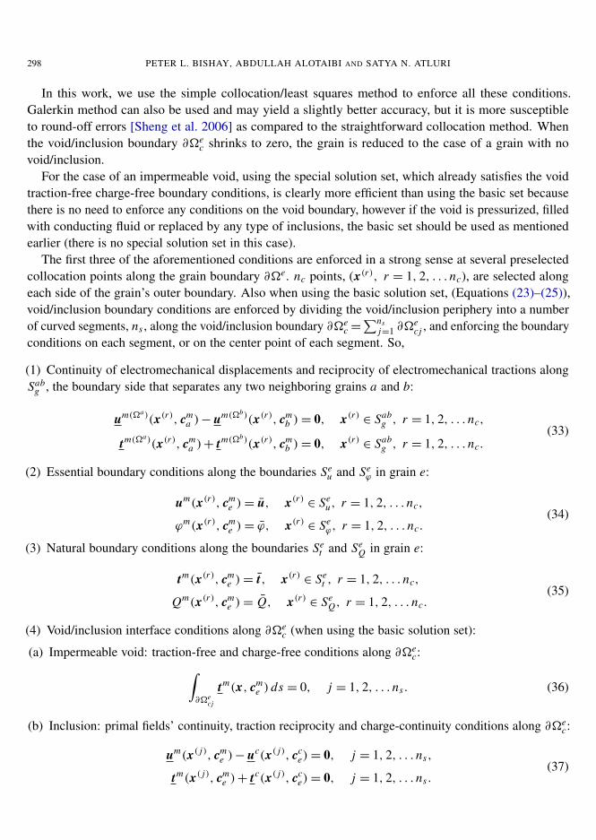
298 PETER L. BISHAY, ABDULLAH ALOTAIBI AND SATYA N. ATLURI

In this work, we use the simple collocation/least squares method to enforce all these conditions.Galerkin method can also be used and may yield a slightly better accuracy, but it is more susceptibleto round-off errors [Sheng et al. 2006] as compared to the straightforward collocation method. Whenthe void/inclusion boundary ∂�e

c shrinks to zero, the grain is reduced to the case of a grain with novoid/inclusion.

For the case of an impermeable void, using the special solution set, which already satisfies the voidtraction-free charge-free boundary conditions, is clearly more efficient than using the basic set becausethere is no need to enforce any conditions on the void boundary, however if the void is pressurized, filledwith conducting fluid or replaced by any type of inclusions, the basic set should be used as mentionedearlier (there is no special solution set in this case).

The first three of the aforementioned conditions are enforced in a strong sense at several preselectedcollocation points along the grain boundary ∂�e. nc points, (x(r), r = 1, 2, . . . nc), are selected alongeach side of the grain’s outer boundary. Also when using the basic solution set, (Equations (23)–(25)),void/inclusion boundary conditions are enforced by dividing the void/inclusion periphery into a numberof curved segments, ns , along the void/inclusion boundary ∂�e

c=∑ns

j=1 ∂�ecj , and enforcing the boundary

conditions on each segment, or on the center point of each segment. So,

(1) Continuity of electromechanical displacements and reciprocity of electromechanical tractions alongSab

g , the boundary side that separates any two neighboring grains a and b:

um(�a)(x(r), cma )− um(�b)(x(r), cm

b )= 0, x(r) ∈ Sabg , r = 1, 2, . . . nc,

tm(�a)(x(r), cma )+ tm(�b)(x(r), cm

b )= 0, x(r) ∈ Sabg , r = 1, 2, . . . nc.

(33)

(2) Essential boundary conditions along the boundaries Seu and Se

ϕ in grain e:

um(x(r), cme )= u, x(r) ∈ Se

u, r = 1, 2, . . . nc,

ϕm(x(r), cme )= ϕ, x(r) ∈ Se

ϕ, r = 1, 2, . . . nc.(34)

(3) Natural boundary conditions along the boundaries Set and Se

Q in grain e:

tm(x(r), cme )= t, x(r) ∈ Se

t , r = 1, 2, . . . nc,

Qm(x(r), cme )= Q, x(r) ∈ Se

Q, r = 1, 2, . . . nc.(35)

(4) Void/inclusion interface conditions along ∂�ec (when using the basic solution set):

(a) Impermeable void: traction-free and charge-free conditions along ∂�ec:∫

∂�ecj

tm(x, cme ) ds = 0, j = 1, 2, . . . ns . (36)

(b) Inclusion: primal fields’ continuity, traction reciprocity and charge-continuity conditions along ∂�ec:

um(x( j), cme )− uc(x( j), cc

e)= 0, j = 1, 2, . . . ns,

tm(x( j), cme )+ tc(x( j), cc

e)= 0, j = 1, 2, . . . ns .(37)

MTCGS FOR MODELING PIEZOELECTRIC COMPOSITE AND POROUS MATERIALS 299

Combining all these conditions for N grains in a matrix/vector form leads to

Ac= b or c= A−1b, (38)

where c is a column matrix containing the unknown coefficients of the matrix and inclusion of all grains.The length of the vector c can be expressed as

NT =

N∑e=1

((mT )e+ (mT c)e), (39)

where (mT )e is the number of Trefftz functions in the matrix of grain e, and (mT c)e is the number ofTrefftz functions in the inclusion of grain e (if applicable). These numbers depend on M , the highestorder of Zk in (23)–(25) or (29), used in the matrix and inclusion of each grain. In this study, we use thefollowing (according to (26)):

M = 4 (for matrix of a grain with void or inclusion):(mT )e = 6(2M + 1)= 54 (basic solution set, ellipse-exterior domain)

M = 4 (for inclusions):(mT c)e = 6(M + 1)= 30 (basic solution set, ellipse-interior domain)

M = 2 (for matrix of a grain with impermeable void):(mT )e = 6(M + 1)= 18 (special solution set).

Since we are collocating six variables at each collocation point on each of the inner boundaries (bound-aries shared by any two neighboring grains), and three variables at each collocation point on each of theouter boundaries (grain boundaries on the outer frame of the domain), the number of collocation equationscan be expressed as:

NE = nc(6Ni + 3No)+

N∑e=1

pe(ns)e, (40)

where Ni is the number of inner grain boundaries (sides) in the whole domain, No is the number of outergrain boundaries (sides) in the whole domain, and (ns)e is the number of segments used to divide thevoid periphery in grain e (only if the basic solution set is used) or the number of collocation points alongthe inclusion periphery in grain e, and pe = 0 if we are using the special solution set, pe = 3 if grain econtains a void and the basic solution set is used, while pe = 6 if grain e contains an inclusion.

In order for the system of equations (38) to be solved, we need NT ≤ NE . In the last three exampleswe present in Section 7, we use two uniformly distributed collocation points on each side of the outerboundary of each grain (nc = 2) and 16 points or segments on the void/inclusion boundary in each grain((ns)e = 16). This ensures that the number of equations is larger than the number of unknowns; hence thesystem is over-constrained and is solved using singular value decomposition (SVD). The SVD methodcan solve even the singular system of equations and produces the least squares solutions to the over-constrained systems. The distribution of collocation points along each side of a grain’s outer boundarycould be selected as the Gaussian points [Bishay and Atluri 2012]. However this makes no significantdifference in the solution.

300 PETER L. BISHAY, ABDULLAH ALOTAIBI AND SATYA N. ATLURI

5. Multi-region Trefftz collocation grain (MTCG) formulationfor inverse problems with regularization

If both electromechanical displacements and tractions are specified or known only on a part of the prob-lem boundary, the inverse problem is to determine the electromechanical displacements and tractions inthe domain as well as the other part of the boundary where everything is unknown. The same can besaid if “tractions” is replaced by “strains” in the previous sentence. One example is in health monitoringof piezoelectric composites and devices when data are known or measured on the outer boundaries, butnot available at the inaccessible cavities in the domain.

Now let Sec be a part of the boundary of grain e (outer boundaries for a grain containing an inclusion,

and both inner and outer boundaries for a grain with a void) where electromechanical displacementsand tractions (or strains) are known. We use the available data and select enough collocation points(x(p) ∈ Se

c , p = 1, 2, . . . P) along Sec to get

um(x(p), cme )= u, ϕm(x(p), cm

e )= ϕ, p = 1, 2, . . . P, (41)

andtm(x(p), cm

e )= t, Qm(x(p), cme )= Q, p = 1, 2, . . . P, (42)

orεm(x(p), cm

e )= ε, Em(x(p), cme )= E, p = 1, 2, . . . P. (43)

Combining (41) and (42) or (43) in addition to the continuity of electromechanical displacements andreciprocity of electromechanical tractions along Sab

g in (33), and the inclusion boundary conditions in(37) for grains with inclusions, represent the measured or known data in all grains. This can be writtenin matrix form as

AI cI = bI . (44)

This equation cannot be solved directly using the least squares method because the system of equa-tions in inverse problems is known to be ill-posed and generally very-sensitive to perturbation in themeasurement data on the boundary Se

c . Hence, regularization techniques should be used to mitigate thisill-posedness. There are several regularization methods that were used in the literature, among which arethe truncated singular value decomposition (TSVD), selective singular value decomposition (SSVD), andthe Tikhonov regularization [Hansen 1994; Tikhonov and Arsenin 1974]. In this work, TSVD methodwas used and the regularization parameter is obtained using the generalized cross-validation (GCV)method. For details about the aforementioned methods, the reader is referred to [Hansen 1994].

This formulation is generally suitable for any selection of Sec . For a plate with a hole modeled with

only one region (N = e = 1), for instance, Sc could be all or part of the outer boundary where allmeasurements can be taken.

6. On using representative volume element (RVE) to predictthe effective material properties of piezoelectric composites

In order to determine the overall properties of piezoelectric composites from known properties of theirconstituents (matrix and particles or fibers), two approaches were used in the literature: macromechanical

MTCGS FOR MODELING PIEZOELECTRIC COMPOSITE AND POROUS MATERIALS 301

and micromechanical. In the macromechanical approach, the heterogeneous structure of the composite isreplaced by a homogeneous medium with anisotropic properties, while in the micromechanical approach,a periodic RVE or a unit cell model is used to obtain the global properties of the composite [Berger et al.2006]. A unit cell is the smallest part that contains sufficient information on the geometrical and materialparameters at the microscopic level to allow for prediction of the effective properties of the composite.The numerical methods, such as the finite elements, are well-suited to model the RVE and to describethe behavior of these composite materials because there are no restrictions on the geometry, the materialproperties, the number of phases, and the size of the composite constituents. When employing unit cellmodels, the local fields in the constituent phases can be accurately determined by the numerical method,and various mechanisms such as damage initiation and propagation can be studied through the analysis.Numerical homogenization method is based on finding a globally homogeneous medium equivalent tothe original composite, where the strain energy stored in both systems is approximately the same. Inorder to do so, first, a representative volume element which captures the overall behavior of a compositestructure is created. Then the effective material properties are calculated by applying periodic boundaryconditions and appropriate load cases, which are connected to specific deformation patterns, to the unitcell [Kari et al. 2008].

It is known that the advantages of the analytical approaches over the FE analyses are their abilityto model statistical distributions of fibers/particles in the composite, and their low computational time,while the FE analysis, in contrast, is appropriate for estimating the effective properties of composites witha given periodic fiber/particle distribution and more complicated geometries (different shapes of fibers’cross-section, more than two phases, etc.), and at the same time, the local fields can be obtained accurately.Berger et al. [2006] found that in order to get sufficiently accurate results from the FE model, the meshdensity should be chosen in such a way that the average element width is at least 5% of the unit cellwidth. This means that at least 400 two-dimensional regular elements are required to accurately modela two-dimensional unit cell that includes only one fiber or particle. Finite element results are sensitiveto mesh density; hence it could be a difficult task to find appropriate meshes for the RVE [Berger et al.2005]. The disadvantages of the numerical models can be avoided if we resort to the newly developedtechniques such as those presented in this article and in [Bishay and Atluri 2014; Bishay et al. 2014;Dong and Atluri 2012a; 2012b; 2012c; 2012d] because these advanced methods can model a grain withits inclusion using only one element or region whose geometric shape is arbitrary, hence any statisticalrandom distribution of fibers or particles can be accounted for with relatively very small computationalcost and with high resolution in local fields’ calculation.

In Section 7.4, we show the ability of MTCGs method to predict the effective material properties of apiezoelectric composite using only one region, while in Section 7.5, we show the ability of the proposedmethod to model random distributions of the second phase, and to obtain high resolution of local fieldsthat enables studying damage initiation mechanisms in the microlevel.

7. Numerical examples

The formulation described above is programmed using Matlab in a 64-bit Windows operating system,and executed on a PC computer equipped with Intel Q8300 2.5 GHz CPU, and 8 GB RAM. The materialproperties of the materials used in the examples in this section are listed in Table 1.

302 PETER L. BISHAY, ABDULLAH ALOTAIBI AND SATYA N. ATLURI

Property C11 C12 C13 C22 C23 C33 C44 C55

PZT-4 139 77.8 74.3 139 74.3 113 25.3 25.3PZT-7A 148 76.2 74.2 148 74.2 131 25.4 25.4LaRC-SI 8.1 5.4 5.4 8.1 5.4 8.1 1.4 1.4

Property C66 e31 e32 e33 e15 h11 h22 h33

PZT-4 30.6 −6.98 −6.98 13.84 13.44 6 6 5.47PZT-7A 35.9 460 460 235 9.2 −2.1 −2.1 9.5LaRC-SI 1.4 0 0 0 0 2.8 2.8 2.8

Table 1. Material properties used in the numerical examples: Ci j in GPa, ei j in C/m2,hi i in pC/(Vm).

Simple problems that use grains with no voids or inclusions, such as patch test and bending of apiezoelectric panel, can be easily and accurately modeled using any number of grains (with no voids orinclusions) to mesh the problem domain, and the error in the whole structure is less than 1%. Patch testwith any number of grains containing inclusions having the same material properties as that of the matrixcan also be passed with error less than 1%.

In the following, we show some numerical examples using the proposed MTCGs. In the first examplewe present inverse problem where the electromechanical displacements and tractions are all measuredwith white noise on the outer boundary of a piezoelectric domain with an impermeable elliptical voidunder mechanical loading, and the variables on the unreachable void surface are predicted. Then westudy the convergence of this inverse problem as the accessible part on the outer boundary of the domainshrinks. The problem of a piezoelectric inclusion in an infinite piezoelectric matrix is then studied.This is followed by evaluation of material properties of a piezoelectric particulate composite material asfunctions of particle volume fraction. Finally we present contour plots that detect damage-prone sites inporous piezoelectric material samples with arbitrary elliptical voids. Comparisons with other analyticaland computational results are presented whenever possible.

7.1. Piezoelectric panel with impermeable void: inverse problem. Consider a piezoelectric panel withan arbitrarily oriented elliptical void whose semi-axes are a and b and the inclination angle between theelliptical void minor axis and the poling direction is ζ as shown in Figure 2 (left). The local coordinatesystem of the ellipse is denoted x1-x3, while the global coordinate system is denoted X1-X3. The polingdirection is aligned with the global vertical X3 axis (shown in blue in the figure). The material is PZT-4 whose properties are presented in Table 1 (taken from [Xu and Rajapakse 1999]) and plane strainassumption is used in this problem. Now consider that the electromechanical displacements and tractionsare all measured at the outer boundary and that there is some white noise in the measurements. Theinverse problem is to use these available measurements to predict the electromechanical tractions anddisplacements at the inner cavity. In this example, we use the analytical solution presented in [Xu andRajapakse 1999] for an elliptical void in an infinite piezoelectric panel as the prescribed (or measured)data on the outer boundary after adding certain level of white noise. Mechanical load σo = 1 Pa is appliedon the panel’s upper and lower edges. In this example we take L =W = 6a, b/a = 0.6, ζ = 0, M = 4

MTCGS FOR MODELING PIEZOELECTRIC COMPOSITE AND POROUS MATERIALS 303

]

3x

2a 2b

1x

L

oV

oV

W

Poling direction

direction

1X

3X

20

19

18

17

16

15

14

13

12

11

31

32

33

34

35

36

37

38

39

40

L

W 1X

3X

1 2 3 4 5 6 7 8 9 10

30 29 28 27 26 25 24 23 22 21

2a

Side 1

Side 3

Side 2 Side 4

Figure 2. Left: a finite rectangular domain with arbitrarily oriented elliptical void.Right: collocation points considered in Section 7.2.

0 50 100 150−2

−1

0

1

2

3

4

5

θ (degree)

σθ/σ

o

Direct

Inverse

Inverse with SNR = 40 dB

Inverse with SNR = 30 dB

0 50 100 150−0.4

−0.2

0

0.2

0.4

0.6

θ (degree)

Dθ/σ

o [

pC

/N]

Figure 3. Variations of σθ/σo (left), Dθ/σo (right) along the periphery of an elliptical void.

(equivalent to 54 unknown coefficients) and we use 3 collocation points per side (giving 72 collocationequations). Hence, in this case Sc, mentioned in Section 5, is all the outer boundary of the plate whereall data are measured.

Figure 3 and Figure 4 show the computed circumferential distributions of σθ , Dθ , Eθ and Er dividedby σo obtained from the solution of the inverse problem with different levels of white noise added tothe measured electromechanical displacements and tractions. The figures show that when there is nonoise present, this approach can always exactly reproduce the electromechanical tractions in the domain.When white noise of 40 dB and 30 dB signal-to-noise ratio (SNR), which is equivalent to 1% and 3.3%amplitude of noise in the measurements, is added, only limited error is obtained in the predicted stress,electric displacement and electric field on the void periphery.

The effects of varying ζ , a/b and W/a ratios on the stress, electric displacement and electric field arepresented in [Xu and Rajapakse 1998].

304 PETER L. BISHAY, ABDULLAH ALOTAIBI AND SATYA N. ATLURI

0 50 100 150−0.08

−0.06

−0.04

−0.02

0

0.02

0.04

0.06

0.08

θ (degree)

Eθ/σ

o [

m2/C

]

Direct

Inverse

Inverse with SNR = 40 dB

Inverse with SNR = 30 dB

0 50 100 150−0.04

−0.02

0

0.02

0.04

0.06

θ (degree)

Er/σ

o [

m2/C

]

Figure 4. Variations of Eθ/σo (left), Er/σo (right) along the periphery of an elliptical void.

7.2. Convergence study for the inverse problem. In this study, the same problem presented in Section 7.1is considered again when the outer boundary is not fully accessible. Hence we rely on measurementstaken from only a limited part of the outer boundary. Ten collocation points are used along each side of theouter boundary as shown in Figure 2 (right) and we keep removing collocation equations correspondingto these points from side 2 first (starting from point 11 in the figure) followed by side 3, then side 4.Every time we remove two points, we solve the problem and calculate the discrete extreme mechanicaland electrical errors, expressed as

Emech = maxxr∈∂�c

(|σθ (xr )− σθ (xr )|

σmax

), Eelect = max

xr∈∂�c

(|Dθ (xr )− Dθ (xr )|

Dmax

), (45)

where σθ (xr ) and Dθ (xr ) are the exact solutions at boundary points xr along the periphery of the void;σmax and Dmax are respectively the maximum magnitudes of σθ (xr ) and Dθ (xr ).

It was found that when there is no noise in the prescribed (measured) data, only nine points (equivalentto 54 collocation equations, which is equal to the number of unknown coefficients when M = 4 is used)are required to get accurate results with Emech and Eelect less than 0.001. These nine points could beprescribed on only a small part (quarter) of side 1 only, side 3 only, or on both sides 2 and 4 such that atleast one point is on one of these two sides and the remaining points are on the other side. However whenthere is a white noise in the prescribed (measured) data, errors increase as we remove more points (or takeour measurements from only a limited part of the outer boundary). The mechanical and electrical discreteextreme errors are presented in Table 2, when white noise of 40 dB signal-to-noise ratio (SNR) is addedto the prescribed data, as more points are removed from the collocation points in Figure 2. It is clearfrom the table that the errors increase as more collocation points are removed from the outer boundary.When all collocation points on side 2 are not used, we get Emech ≈ 3%, and Eelect ≈ 12%. When allcollocation points on both side 2 and side 3 are not used, we get Emech ≈ 17.5%, and Eelect ≈ 51%.Removing additional points from side 4, results in highly increasing Eelect.

It should be noted that the numbers in Table 2 change slightly every time we change the added randomwhite noise. In addition, errors increase as the noise level increases.

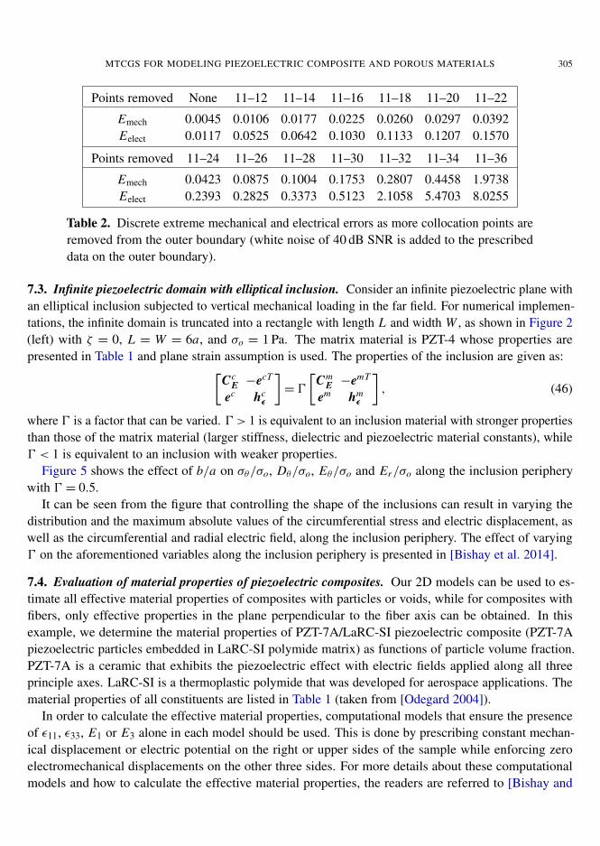
MTCGS FOR MODELING PIEZOELECTRIC COMPOSITE AND POROUS MATERIALS 305

Points removed None 11–12 11–14 11–16 11–18 11–20 11–22

Emech 0.0045 0.0106 0.0177 0.0225 0.0260 0.0297 0.0392Eelect 0.0117 0.0525 0.0642 0.1030 0.1133 0.1207 0.1570

Points removed 11–24 11–26 11–28 11–30 11–32 11–34 11–36

Emech 0.0423 0.0875 0.1004 0.1753 0.2807 0.4458 1.9738Eelect 0.2393 0.2825 0.3373 0.5123 2.1058 5.4703 8.0255

Table 2. Discrete extreme mechanical and electrical errors as more collocation points areremoved from the outer boundary (white noise of 40 dB SNR is added to the prescribeddata on the outer boundary).

7.3. Infinite piezoelectric domain with elliptical inclusion. Consider an infinite piezoelectric plane withan elliptical inclusion subjected to vertical mechanical loading in the far field. For numerical implemen-tations, the infinite domain is truncated into a rectangle with length L and width W , as shown in Figure 2(left) with ζ = 0, L = W = 6a, and σo = 1 Pa. The matrix material is PZT-4 whose properties arepresented in Table 1 and plane strain assumption is used. The properties of the inclusion are given as:[

CcE −ecT

ec hcε

]= 0

[Cm

E −emT

em hmε

], (46)

where 0 is a factor that can be varied. 0 > 1 is equivalent to an inclusion material with stronger propertiesthan those of the matrix material (larger stiffness, dielectric and piezoelectric material constants), while0 < 1 is equivalent to an inclusion with weaker properties.

Figure 5 shows the effect of b/a on σθ/σo, Dθ/σo, Eθ/σo and Er/σo along the inclusion peripherywith 0 = 0.5.

It can be seen from the figure that controlling the shape of the inclusions can result in varying thedistribution and the maximum absolute values of the circumferential stress and electric displacement, aswell as the circumferential and radial electric field, along the inclusion periphery. The effect of varying0 on the aforementioned variables along the inclusion periphery is presented in [Bishay et al. 2014].

7.4. Evaluation of material properties of piezoelectric composites. Our 2D models can be used to es-timate all effective material properties of composites with particles or voids, while for composites withfibers, only effective properties in the plane perpendicular to the fiber axis can be obtained. In thisexample, we determine the material properties of PZT-7A/LaRC-SI piezoelectric composite (PZT-7Apiezoelectric particles embedded in LaRC-SI polymide matrix) as functions of particle volume fraction.PZT-7A is a ceramic that exhibits the piezoelectric effect with electric fields applied along all threeprinciple axes. LaRC-SI is a thermoplastic polymide that was developed for aerospace applications. Thematerial properties of all constituents are listed in Table 1 (taken from [Odegard 2004]).

In order to calculate the effective material properties, computational models that ensure the presenceof ε11, ε33, E1 or E3 alone in each model should be used. This is done by prescribing constant mechan-ical displacement or electric potential on the right or upper sides of the sample while enforcing zeroelectromechanical displacements on the other three sides. For more details about these computationalmodels and how to calculate the effective material properties, the readers are referred to [Bishay and

306 PETER L. BISHAY, ABDULLAH ALOTAIBI AND SATYA N. ATLURI

0 20 40 60 80−0.5

0

0.5

1

1.5

2

θ (rad)

σθ/σ

o

b/a=0.7

b/a=1

b/a=1.3

0 20 40 60 80−0.08

−0.06

−0.04

−0.02

0

0.02

0.04

θ (rad)

Dθ/σ

o [

pC

/N]

b/a=0.7

b/a=1

b/a=1.3

0 20 40 60 80−0.04

−0.03

−0.02

−0.01

0

0.01

θ (rad)

Eθ/σ

o [

m2/C

]

b/a=0.7

b/a=1

b/a=1.3

0 20 40 60 80−0.025

−0.02

−0.015

−0.01

−0.005

0

0.005

θ (rad)

Er/σ

o [

m2/C

]

b/a=0.7

b/a=1

b/a=1.3

Figure 5. Effect of b/a on σθ/σo (top left), Dθ/σo (top right), Eθ/σo (bottom left) andEr/σo (bottom right) along the inclusion periphery.

Atluri 2014]. Here we just present the results. The three Young’s moduli Y1, Y2 and Y3 can be obtainedfrom the stiffness matrix constants Ci j .

The RVE used is composed of just one region (grain) that includes an inclusion. Plane strain assump-tion is used in this study and the direction of polarization is vertically upward.

Figure 6 shows the predictions of the different effective material constants as functions of particlevolume fraction and compared with Mori–Tanaka (MT), self-consistent (SC), finite element models usingANSYS (with large number of elements) and Odegard’s proposed analytical model, all presented in[Odegard 2004].

It can be seen that, using only one MTCG, the proposed model gives very accurate predictions ascompared to those of Mori–Tanaka’s model. It is known that the self-consistent model deviates fromMori–Tanaka’s model and gives unrealistic predictions as the volume fraction increases. The proposedmethod is much more computationally efficient as well as numerically more accurate than the simplefinite element models (FEM) using ANSYS, and can be used to model piezo-composites even if thearrangement of particles is not symmetrical which is the main assumption used in all the previouslymentioned analytical models.

7.5. Damage detection in porous piezoelectric materials with arbitrary oriented elliptical voids. Weconsider a porous piezoelectric RVE made of 20 PZT-4 piezoelectric grains with arbitrary sized elliptical

MTCGS FOR MODELING PIEZOELECTRIC COMPOSITE AND POROUS MATERIALS 307

0 0.1 0.2 0.3 0.40

5

10

15

Volume fraction

Y1 =

Y2 [G

Pa]

FEM

Odegard

MT

SC

MTCG

0 0.1 0.2 0.3 0.40

5

10

15

Volume fraction

Y3 [G

Pa]

FEM

Odegard

MT

SC

MTCG

0 0.1 0.2 0.3 0.4−0.04

−0.02

0

0.02

0.04

0.06

0.08

0.1

Volume fraction

e3

1 =

e3

2 [C

/m2]

FEM

Odegard

MT

SC

MTCG

0 0.1 0.2 0.3 0.4−0.005

0

0.005

0.01

0.015

0.02

0.025

0.03

Volume fraction

e3

3 [C

/m2]

FEM

Odegard

MT

SC

MTCG

0 0.1 0.2 0.3 0.40

0.05

0.1

0.15

0.2

0.25

0.3

0.35

Volume fraction

h1

1 =

h2

2 [nF

/m]

FEM

Odegard

MT

SC

MTCG

0 0.1 0.2 0.3 0.40

0.05

0.1

0.15

0.2

0.25

0.3

0.35

0.4

Volume fraction

h3

3 [nF

/m]

FEM

Odegard

MT

SC

MTCG

Figure 6. Predictions of effective piezoelectric material properties of PZT-7A/LaRC-SIas functions of particle volume fraction.

voids whose b/a ratios are in the range of 0.7–1.3. The dimensions of the RVE are L = W = 1 mmand the porosity volume fraction is 0.05. The direction of polarization is vertically upward in all grains.The lower edge is prevented from motion in the vertical direction while the lower left corner node iselectrically grounded and constrained in the horizontal direction. A mechanical loading σo = 1 GPa is

308 PETER L. BISHAY, ABDULLAH ALOTAIBI AND SATYA N. ATLURI

Figure 7. Porous piezoelectric material under mechanical loading: contour plot for prin-cipal stress (upper), strain energy density (lower left), and dielectric energy density (lowerright).

applied on the upper edge. Contour plots of maximum principal stress, strain energy density (SED), aswell as dielectric energy density are shown in Figure 7.

As can be seen from the figures, high principal stress and strain energy density concentrations areobserved near the cavities, in the direction perpendicular to the loading direction. On the other hand, atthe locations near the voids, in the direction parallel to the loading direction, low stress and strain energydensity values are observed. Higher stress and strain energy density concentrations can be observedaround voids that have lower values of b/a (because these voids are sharper and are approaching the

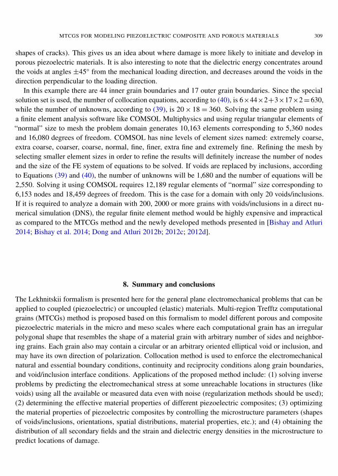
MTCGS FOR MODELING PIEZOELECTRIC COMPOSITE AND POROUS MATERIALS 309

shapes of cracks). This gives us an idea about where damage is more likely to initiate and develop inporous piezoelectric materials. It is also interesting to note that the dielectric energy concentrates aroundthe voids at angles ±45◦ from the mechanical loading direction, and decreases around the voids in thedirection perpendicular to the loading direction.

In this example there are 44 inner grain boundaries and 17 outer grain boundaries. Since the specialsolution set is used, the number of collocation equations, according to (40), is 6×44×2+3×17×2= 630,while the number of unknowns, according to (39), is 20× 18= 360. Solving the same problem usinga finite element analysis software like COMSOL Multiphysics and using regular triangular elements of“normal” size to mesh the problem domain generates 10,163 elements corresponding to 5,360 nodesand 16,080 degrees of freedom. COMSOL has nine levels of element sizes named: extremely coarse,extra coarse, coarser, coarse, normal, fine, finer, extra fine and extremely fine. Refining the mesh byselecting smaller element sizes in order to refine the results will definitely increase the number of nodesand the size of the FE system of equations to be solved. If voids are replaced by inclusions, accordingto Equations (39) and (40), the number of unknowns will be 1,680 and the number of equations will be2,550. Solving it using COMSOL requires 12,189 regular elements of “normal” size corresponding to6,153 nodes and 18,459 degrees of freedom. This is the case for a domain with only 20 voids/inclusions.If it is required to analyze a domain with 200, 2000 or more grains with voids/inclusions in a direct nu-merical simulation (DNS), the regular finite element method would be highly expensive and impracticalas compared to the MTCGs method and the newly developed methods presented in [Bishay and Atluri2014; Bishay et al. 2014; Dong and Atluri 2012b; 2012c; 2012d].

8. Summary and conclusions

The Lekhnitskii formalism is presented here for the general plane electromechanical problems that can beapplied to coupled (piezoelectric) or uncoupled (elastic) materials. Multi-region Trefftz computationalgrains (MTCGs) method is proposed based on this formalism to model different porous and compositepiezoelectric materials in the micro and meso scales where each computational grain has an irregularpolygonal shape that resembles the shape of a material grain with arbitrary number of sides and neighbor-ing grains. Each grain also may contain a circular or an arbitrary oriented elliptical void or inclusion, andmay have its own direction of polarization. Collocation method is used to enforce the electromechanicalnatural and essential boundary conditions, continuity and reciprocity conditions along grain boundaries,and void/inclusion interface conditions. Applications of the proposed method include: (1) solving inverseproblems by predicting the electromechanical stress at some unreachable locations in structures (likevoids) using all the available or measured data even with noise (regularization methods should be used);(2) determining the effective material properties of different piezoelectric composites; (3) optimizingthe material properties of piezoelectric composites by controlling the microstructure parameters (shapesof voids/inclusions, orientations, spatial distributions, material properties, etc.); and (4) obtaining thedistribution of all secondary fields and the strain and dielectric energy densities in the microstructure topredict locations of damage.

310 PETER L. BISHAY, ABDULLAH ALOTAIBI AND SATYA N. ATLURI

Acknowledgements

This work was funded by the Deanship of Scientific Research (DSR), King Abdulaziz University, undergrant number (3-130-35-HiCi). The authors, therefore, acknowledge the technical and financial supportof KAU. This research is also supported in part by the Mechanics Section, Vehicle Technology Division,of the US Army Research Labs, under a collaborative research agreement with UCI. The encouragementof Dy Le and Jaret Riddick is thankfully acknowledged.

References

[Araki and Halloran 2005] K. Araki and J. W. Halloran, “Porous ceramic with interconnected pore channels by a novel freezecasting technique”, J. Am. Ceram. Soc. 88:5 (2005), 1108–1114.

[Berger et al. 2005] H. Berger, S. Kari, U. Gabbert, R. Rodriguez-Ramos, R. Guinovart-Díaz, J. A. Otero, and J. Bravo-Castillero, “An analytical and numerical approach for calculating effective material coefficients of piezoelectric fiber compos-ites”, Int. J. Solids Struct. 42 (2005), 5692–5714.

[Berger et al. 2006] H. Berger, S. Kari, U. Gabbert, R. Rodriguez-Ramos, J. Bravo-Castillero, R. Guinovart-Díaz, F. J. Sabina,and G. A. Maugin, “Unit cell models of piezoelectric fiber composites for numerical and analytical calculation of effectiveproperties”, Smart Mater. Struct. 15 (2006), 451–458.

[Bishay and Atluri 2012] P. L. Bishay and S. N. Atluri, “High-performance 3D hybrid/mixed, and simple 3D Voronoi cellfinite elements, for macro- & micro-mechanical modeling of solids, without using multi-field variational principles”, Comput.Model. Eng. Sci. 84:1 (2012), 41–97.

[Bishay and Atluri 2013] P. L. Bishay and S. N. Atluri, “2D and 3D multiphysics Voronoi cells, based on radial basis functions,for direct mesoscale numerical simulation (DMNS) of the switching phenomena in ferroelectric polycrystalline materials”,Comput. Mater. Continua 33:1 (2013), 19–62.

[Bishay and Atluri 2014] P. L. Bishay and S. N. Atluri, “Trefftz–Lekhnitski grains (TLGs) for efficient direct numerical simu-lation (DNS) of the micro/meso mechanics of porous piezoelectric materials”, Comput. Mater. Sci. 83 (2014), 235–249.

[Bishay et al. 2014] P. L. Bishay, L. Dong, and S. N. Atluri, “Multi-physics computational grains (MPCGs) for direct nu-merical simulation (DNS) of piezoelectric composite/porous materials and structures”, Comput. Mech. (2014). Accepted forpublication.

[Cao et al. 2013] C. Cao, A. Yu, and Q.-H. Qin, “A new hybrid finite element approach for plane piezoelectricity with defects”,Acta Mech. 224:1 (2013), 41–61.

[Chung and Ting 1996] M. Y. Chung and T. C. T. Ting, “Piezoelectric solid with an elliptic inclusion or hole”, Int. J. SolidsStruct. 33:23 (1996), 3343–3361.

[Dong and Atluri 2012a] L. Dong and S. N. Atluri, “A simple multi-source-point Trefftz method for solving direct/inverseSHM problems of plane elasticity in arbitrary multiply-connected domains”, Comput. Model. Eng. Sci. 85:1 (2012), 1–43.

[Dong and Atluri 2012b] L. Dong and S. N. Atluri, “T-Trefftz Voronoi cell finite elements with elastic/rigid inclusions or voidsfor micromechanical analysis of composite and porous materials”, Comput. Model. Eng. Sci. 83:2 (2012), 183–220.

[Dong and Atluri 2012c] L. Dong and S. N. Atluri, “Development of 3D T-Trefftz Voronoi cell finite elements with/withoutspherical voids &/or elastic/rigid inclusions for micromechanical modeling of heterogeneous materials”, Comput. Mater. Con-tinua 29:2 (2012), 169–211.

[Dong and Atluri 2012d] L. Dong and S. N. Atluri, “Development of 3D Trefftz Voronoi cells with ellipsoidal voids &/orelastic/rigid inclusions for micromechanical modeling of heterogeneous materials”, Comput. Mater. Continua 30:1 (2012),39–82.

[Dong and Atluri 2012e] L. Dong and S. N. Atluri, “SGBEM (using non-hyper-singular traction BIE), and super elements, fornon-collinear fatigue-growth analyses of cracks in stiffened panels with composite-patch repairs”, Comput. Model. Eng. Sci.89:5 (2012), 417–458.

MTCGS FOR MODELING PIEZOELECTRIC COMPOSITE AND POROUS MATERIALS 311

[Dong and Atluri 2013] L. Dong and S. N. Atluri, “SGBEM Voronoi cells (SVCs), with embedded arbitrary-shaped inclusions,voids, and/or cracks, for micromechanical modeling of heterogeneous materials”, Comput. Mater. Continua 33:2 (2013), 111–154.

[Hansen 1994] P. C. Hansen, “Regularization tools: a Matlab package for analysis and solution of discrete ill-posed problems”,Numer. Algorithms 6:1-2 (1994), 1–35.

[Jin et al. 2003] D. R. Jin, Z. Y. Meng, and F. Zhou, “Mechanism of resistivity gradient in monolithic PZT ceramics”, Mater.Sci. Eng. B 99 (2003), 83–87.

[Kari et al. 2008] S. Kari, H. Berger, and U. Gabbert, “Numerical evaluation of effective material properties of piezoelectricfibre composites”, pp. 109–120 in Micro-macro-interactions: in structured media and particle systems, edited by A. Bertramand J. Tomas, Springer, Berlin, 2008.

[Klicker et al. 1981] K. A. Klicker, J. V. Biggers, and R. E. Newnham, “Composites of PZT and epoxy for hydrostatic transducerapplications”, J. Am. Ceram. Soc. 64 (1981), 5–9.

[Kumar et al. 2006] B. P. Kumar, H. H. Kumar, and D. K. Kharat, “Effect of porosity on dielectric properties and microstructureof porous PZT ceramics”, Mater. Sci. Eng. B 127 (2006), 130–133.

[Lekhnitskii 1957] S. G. Lekhnitskii, Anizotropnye plastinki, 2nd ed., Gostekhidat, Moscow, 1957. Translated asAnisotropic plates, Gordon and Breach, New York, 1968.

[Lekhnitskii 1977] S. G. Lekhnitskii, Teori� uprugosti anizotroinogo tela, 2nd ed., Nauka, Moscow, 1977. Trans-lated as Theory of elasticity of an anisotropic body, Mir, Moscow, 1981.

[Li et al. 2001] J. F. Li, K. Takagi, N. Terakubo, and R. Watanabe, “Electrical and mechanical properties of piezoelectricceramic/metal composites in the Pb(Zr,Ti)O3/Pt system”, Appl. Phys. Lett. 79 (2001), 2441–2443.

[Li et al. 2003] J. F. Li, K. Takagi, M. Ono, W. Pan, R. Watanabe, and A. Almajid, “Fabrication and evaluation of porouspiezoelectric ceramics and porosity-graded piezoelectric actuators”, J. Am. Ceram. Soc. 86 (2003), 1094–1098.

[Lu and Williams 1998] P. Lu and F. W. Williams, “Green functions of piezoelectric material with an elliptic hole or inclusion”,Int. J. Solids Struct. 35 (1998), 651–664.

[Moorthy and Ghosh 1996] S. Moorthy and S. Ghosh, “A model for analysis of arbitrary composite and porous microstructureswith Voronoi cell finite elements”, Int. J. Numer. Methods Eng. 39 (1996), 2363–2398.

[Odegard 2004] G. M. Odegard, “Constitutive modeling of piezoelectric polymer composites”, Acta Mater. 52:18 (2004),5315–5330.

[Piltner 1985] R. Piltner, “Special finite elements with holes and internal cracks”, Int. J. Numer. Methods Eng. 21:8 (1985),1471–1485.

[Piltner 2008] R. Piltner, “Some remarks on finite elements with an elliptic hole”, Finite Elem. Anal. Des. 44:12-13 (2008),767–772.

[Sheng et al. 2006] N. Sheng, K. Y. Sze, and Y. K. Cheung, “Trefftz solutions for piezoelectricity by Lekhnitskii’s formalismand boundary collocation method”, Int. J. Numer. Methods Eng. 65 (2006), 2113–2138.

[Sosa 1991] H. Sosa, “Plane problems in piezoelectric media with defects”, Int. J. Solids Struct. 28:4 (1991), 491–505.

[Stroh 1958] A. N. Stroh, “Dislocations and cracks in anisotropic elasticity”, Philos. Mag. (8) 3:30 (1958), 625–646.

[Tikhonov and Arsenin 1974] A. N. Tikhonov and V. Y. Arsenin, Metody rexeni� nekorrektnyh zadaq, Nauka,Moscow, 1974. Translated as Solutions of ill-posed problems, Winston, Washington, DC, 1977.

[Wang and Qin 2012] H. Wang and Q.-H. Qin, “A new special element for stress concentration analysis of a plate with ellipticalholes”, Acta Mech. 223:6 (2012), 1323–1340.

[Wang et al. 2004] X. W. Wang, Y. Zhou, and W. L. Zhou, “A novel hybrid finite element with a hole for analysis of planepiezoelectric medium with defects”, Int. J. Solids Struct. 41 (2004), 7111–7128.

[Xu and Rajapakse 1998] X. L. Xu and R. K. N. D. Rajapakse, “Boundary element analysis of piezoelectric solids with defects”,Compos. B Eng. 29:5 (1998), 655–669.

[Xu and Rajapakse 1999] X. L. Xu and R. K. N. D. Rajapakse, “Analytical solution for an arbitrarily oriented void/crack andfracture of piezoceramics”, Acta Mater. 47 (1999), 1735–1747.

312 PETER L. BISHAY, ABDULLAH ALOTAIBI AND SATYA N. ATLURI

[Zhang and Katsube 1995] J. Zhang and N. Katsube, “A hybrid finite element method for heterogeneous materials with ran-domly dispersed rigid inclusions”, Int. J. Numer. Methods Eng. 38 (1995), 1635–1653.

[Zhang and Katsube 1997] J. Zhang and N. Katsube, “A polygonal element approach to random heterogeneous media withrigid ellipses or elliptic voids”, Comput. Methods Appl. Mech. Eng. 148 (1997), 225–234.

Received 7 Dec 2013. Revised 10 Apr 2014. Accepted 8 May 2014.

PETER L. BISHAY: PBishay@stmartin.eduCenter for Aerospace Research and Education (CARE), The Henry Samueli School of Engineering,University of California, Irvine, 4200 Engineering Gateway, Irvine, CA 92697, United States

and

The Hal and Inge Marcus School of Engineering, Saint Martin’s University, 5000 Abbey Way SE, OM 329,Lacey, WA 98503-7500, United States

ABDULLAH ALOTAIBI: aalotaibi@kau.edu.saDepartment of Mathematics, Faculty of Sciences, King Abdulaziz University, P.O. Box 80203, Jeddah 21589, Saudi Arabia

SATYA N. ATLURI: satluri@uci.eduCenter for Aerospace Research and Education (CARE), The Henry Samueli School of Engineering,University of California, Irvine, 4200 Engineering Gateway, Irvine, CA 92697, United States

and

Faculty of Engineering, King Abdulaziz University, Jeddah 22254, Saudi Arabia

mathematical sciences publishers msp

JOURNAL OF MECHANICS OF MATERIALS AND STRUCTURESmsp.org/jomms

Founded by Charles R. Steele and Marie-Louise Steele

EDITORIAL BOARD

ADAIR R. AGUIAR University of São Paulo at São Carlos, BrazilKATIA BERTOLDI Harvard University, USA

DAVIDE BIGONI University of Trento, ItalyIWONA JASIUK University of Illinois at Urbana-Champaign, USA

THOMAS J. PENCE Michigan State University, USAYASUHIDE SHINDO Tohoku University, JapanDAVID STEIGMANN University of California at Berkeley

ADVISORY BOARD

J. P. CARTER University of Sydney, AustraliaR. M. CHRISTENSEN Stanford University, USAG. M. L. GLADWELL University of Waterloo, Canada

D. H. HODGES Georgia Institute of Technology, USAJ. HUTCHINSON Harvard University, USA

C. HWU National Cheng Kung University, TaiwanB. L. KARIHALOO University of Wales, UK

Y. Y. KIM Seoul National University, Republic of KoreaZ. MROZ Academy of Science, Poland

D. PAMPLONA Universidade Católica do Rio de Janeiro, BrazilM. B. RUBIN Technion, Haifa, Israel

A. N. SHUPIKOV Ukrainian Academy of Sciences, UkraineT. TARNAI University Budapest, Hungary

F. Y. M. WAN University of California, Irvine, USAP. WRIGGERS Universität Hannover, Germany

W. YANG Tsinghua University, ChinaF. ZIEGLER Technische Universität Wien, Austria

PRODUCTION production@msp.org

SILVIO LEVY Scientific Editor

See msp.org/jomms for submission guidelines.

JoMMS (ISSN 1559-3959) at Mathematical Sciences Publishers, 798 Evans Hall #6840, c/o University of California, Berkeley,CA 94720-3840, is published in 10 issues a year. The subscription price for 2014 is US $555/year for the electronic version, and$710/year (+$60, if shipping outside the US) for print and electronic. Subscriptions, requests for back issues, and changes of addressshould be sent to MSP.

JoMMS peer-review and production is managed by EditFLOW® from Mathematical Sciences Publishers.

PUBLISHED BY

mathematical sciences publishersnonprofit scientific publishing

http://msp.org/© 2014 Mathematical Sciences Publishers

Journal of Mechanics of Materials and StructuresVolume 9, No. 3 May 2014

B-splines collocation eigenanalysis of 2D acoustic problemsCHRISTOPHER G. PROVATIDIS 259

Multi-region Trefftz collocation grains (MTCGs) for modeling piezoelectriccomposite and porous materials in direct and inverse problemsPETER L. BISHAY, ABDULLAH ALOTAIBI and SATYA N. ATLURI 287

Analytical solution for ductile and FRC plates on elastic ground loaded on a smallcircular area ENRICO RADI and PIETRO DI MAIDA 313

Solution of a receding contact problem using an analytical method and a finiteelement method ERDAL ÖNER, MURAT YAYLACI and AHMET BIRINCI 333

Sliding of a cup-shaped die on a half-space: influence of thermal relaxation,convection and die temperature LOUIS MILTON BROCK 347

JournalofMechanics

ofMaterials

andStructures

2014V

ol.9,No.3