Numerical study of the blade cooling effect generated by multiple jets issuing

at different angles and speed into a compressible horizontal cross flow.

MECH 523Applied CFD

Sagar Kapadia

Content Industrial Applications Geometry, Grid and Design Parameters Governing Equations (N-S) And Solver –

Cobalt Finite Volume Method Turbulence Model (DES) Results And Discussion Conclusion and Future Scope

Industrial Applications Take off and landing

engineering Film cooling of Turbine blades Jets into combustors

0.2m

0.9m

0.2m

Geometry

Hot Crossflow

Cool

Jet

Design Variables(1) Blowing Ratio(R) =

where, 'h' stands for the hole,and 's' for the source. Three different values of R (1, 2, 2.5) has been used.

(2) Angle of Att

h h

s s

uu

o oack ( )

Two different values of (20 , 35 ) has been used

Grid Information Grid has been created using Gridgen-

14.03 preprocessor. Grid information:

Unstructured Grid Number of nodes = 121316 Number of elements = 651499 Element Type – Tetrahedran Quality of the grid = 99.78 %

(Blacksmith)

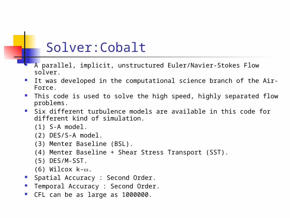
Solver:Cobalt A parallel, implicit, unstructured Euler/Navier-Stokes Flow solver. It was developed in the computational science branch of the Air-Force. This code is used to solve the high speed, highly separated flow

problems. Six different turbulence models are available in this code for different

kind of simulation.(1) S-A model.(2) DES/S-A model.(3) Menter Baseline (BSL).(4) Menter Baseline + Shear Stress Transport (SST).(5) DES/M-SST.(6) Wilcox k-.

Spatial Accuracy : Second Order. Temporal Accuracy : Second Order. CFL can be as large as 1000000.

^ ^ ^ ^ ^ ^ ^ ^( ). ( ).

v

QdV f i g j h k n d r i g j t k n dt

uQ v

we

2

( )

uu p

f uvuw

u e p

2

( )

vuv

g v pvw

v e p

2

( )

wuw

h vww p

w e p

0 0 0

xx xy xz

xy yy yz

xz yz zz

r s t

a b c

, , ;xx xy xz x xy yy yz y xz yz zz zHere a u v w k b u v w k and c u v w k

Governing equation for this case is unsteady, compressible Navier-Stokesequation. In integral form, it can be written as following:

where, is the fluid element volume; is the fluid element surface area; i, j,k are the Cartesian

unit vectors and is the unit normal to .

Governing Equation

. . . .

. . . .

. . . .. . . ..

w x

y z

i,j

i,j-1/2

i,j+1/2

i+1/2,j i-1/2,j

Finite Volume Method

x

y

2-D Problem : 0

Integrating theequation over the volume 'wxyz ',

0 0

where, ( )( )(1)

Applying Green'sTheorem,

(1) . 0

wxyz

wxyz wxy

U F Gt x y

U F Gd

t x yd dx dy

U dxdy H ndSt

where,n is the unit normal to thesurfaceSof the finite volumeand H can beexpressed

in Cartesian coordinates as

For the 2-D geometry,. ( )(1)

z

i jH F G

H ndS Edy Fdx

i+1/2,j.

w x

y z

i,j

i,j-1/2

i,j+1/2

i-1/2,j

Discretization

Discretization

1, ,

, 1/ 2 1/ 2, , 1/ 2 1/ 2,

, 1/ 2 1/ 2, , 1

( ) 0

which can be written as,

( )

(

wxyz wxyz

n ni j i j

wxyz i j ab i j bc i j cd i j da

i j ab i j bc i j

Udxdy Fdy Gdxt

U US F y F y F y F y

t

G x G x G

/ 2 1/ 2,

12 1 2

,

) 0

Area of thecell

Average valueof Uin thecell

, Flux Vectors,calculated either explicitly(n) or implicitly(n+1) , depends on thealgorithm

cd i j da

wxyz

i j

x G x

x x xS

U

F G

Boundary

Implementation of Boundary Condition in Finite Volume

•P1=P2,•u1 = -u2 (No-Slip Condition)•v1 = -v2•T1=T2 (Adiabatic)

i,j+1/2.x

y z

1

w1

y1

.x1

z1

2

Mirror Cellw

InputsTypeBoundary Condition

Static Pressure = 101325 PaPressure Outlet

Outlet

Symmetric Wall (Gradient of all physical quantity is zero).

SymmetrySymmetry

P, T, Mach Number, Turbulent Viscosity(Ref. Condition)

FarfieldOpen Faces

No-Slip ConditionAdiabatic WallBlade

Density,Velocity profile (depends on R), P, Turbulence Viscosity

User-DefinedHole

P, T= 3000K, Mach Number=0.3, Turbulence Viscosity

SourceInlet

Model Boundary Conditions

Turbulence Model :Detached Eddy Simulation (DES)

Purpose of DES – To overcome the disadvantages of LES and RANS Hybrid Turbulence Model of, (1) RANS and (2) LES Used for High Speed, Massively separated flows . RANS - Attached Boundary Layers

LES - Separated Regions. Presently available definition of DES is not related with any particular

turbulence model. DEFINITION : DES is a 3-D unsteady numerical solution using single

turbulence model which functions as a sub-grid scale model in the regions where grid density is fine enough for LES and as a RANS where it is not.

“fine enough” – when maximum spatial step,is much smaller than the flow turbulence length scale,

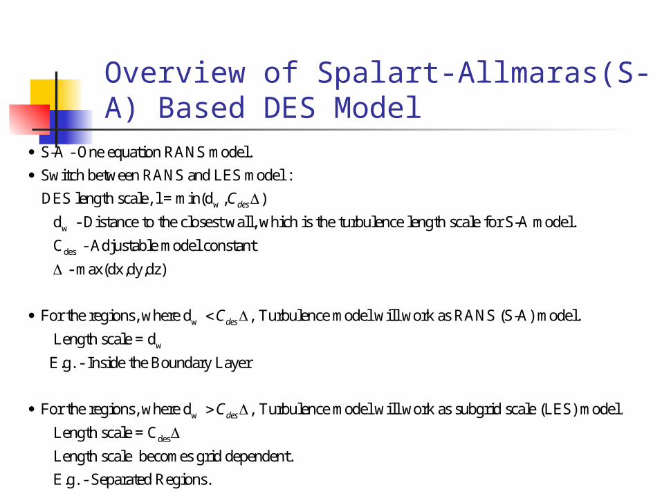
Overview of Spalart-Allmaras(S-A) Based DES Model

w

w

S-A - One equation RANS model. Switch between RANS and LES model :

DES length scale, l = min(d , ) d - Distance to the closest wall, which is the turbulence length scale for S-A model.

desC

des

w

w

C - Adjustable model constant - max(dx,dy,dz)

For the regions, where d , Turbulence model will work as RANS (S-A) model. Length scale = d E.g. - Inside the Boundary La

desC

w

des

yer

For the regions, where d , Turbulence model will work as subgrid scale (LES) model. Length scale = C Length scale becomes grid dependent. E.g. - Separated Regions.

desC

Flow Visualization-Temperature Distribution (400 time steps)

Flow Visualization-Vortex Formation

Temperature Contours for R =1 and = 35o

x = 0.297561

x = 0.465534

Temperature Contours forR =2.50 and = 20o

x = 0.5121495

Temperature Contours for R = 2 and = 20o

Cooling Effect Obtained by the recirculation of the cold air

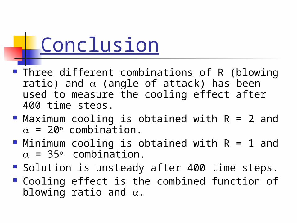
Conclusion Three different combinations of R (blowing

ratio) and (angle of attack) has been used to measure the cooling effect after 400 time steps.

Maximum cooling is obtained with R = 2 and = 20o combination.

Minimum cooling is obtained with R = 1 and = 35o combination.

Solution is unsteady after 400 time steps. Cooling effect is the combined function of

blowing ratio and .

Future Scope To solve the problem with more

combinations of R and . To get the steady state solution for

the cases described in the presentation and compare the cooling.

To find out the optimum combination of Blowing Ratio and Angle of attack of the jet for maximum cooling.