Meccanica e Scienze Avanzate dell’Ingegneria...
110
Alma Mater Studiorum – Università di Bologna DOTTORATO DI RICERCA IN Meccanica e Scienze Avanzate dell’Ingegneria Curriculum Meccanica Applicata Ciclo XXVI Settore Concorsuale di afferenza: 09/A2 Settore Scientifico disciplinare: ING-IND/13 Displacement Analysis of Under-Constrained Cable-Driven Parallel Robots Presentata da: Ghasem Abbasnejad Matikolaei Relatore della Tesi: Ing. Marco Carricato Coordinatore della Scuola di Dottorato: Prof. Vincenzo Parenti Castelli Esame finale anno 2014
Transcript of Meccanica e Scienze Avanzate dell’Ingegneria...
AAllmmaa MMaatteerr SSttuuddiioorruumm –– UUnniivveerrssiittàà ddii BBoollooggnnaaDOTTORATO DI RICERCA INMeccanica e Scienze Avanzate dell’IngegneriaCurriculum Meccanica ApplicataCiclo XXVI
Settore Concorsuale di afferenza: 09/A2
Settore Scientifico disciplinare: ING-IND/13
Displacement Analysis ofUnder-Constrained Cable-Driven Parallel Robots
Presentata da:Ghasem Abbasnejad MatikolaeiRelatore della Tesi:Ing. Marco CarricatoCoordinatore della Scuola di Dottorato:Prof. Vincenzo Parenti Castelli
Esame finale anno 2014
Displacement Analysis of Under-ConstrainedCable-Driven Parallel Robots
Ghasem Abbasnejad
Department of Industrial Engineering
University of Bologna
A thesis submitted for the degree of
Doctor of Philosophy

I would like to dedicate this thesis to:the memory of my father;
and my mother.

Acknowledgements
I would like to express my deepest gratitude to my supervisor, Dr. Marco Carricato, for ac-cepting me to work with him and providing me with the opportunity to undertaken researchon this topic. I am indebted to him for sharing his invaluable expertise in kinematics androbotics with me. I could not have imagined completing this thesis without his guidanceand support.
I would also like to extend my appreciation to Prof. Vincenzo Parenti Castelli for warmlyaccepting me as a member of his research group, for his support and for providing me withall the facilities necessary to complete this thesis.
I would like to thank all of my colleagues in GRAB (Group of Robotics and ArticularBiomechanics). It was a great pleasure working with all of them. Their support, not onlyas colleagues but also as friends, made me feel at home despite being outside my countryof origin.
I am also very grateful to Adrian Lutey for his help in editing the use of English in thisthesis.
I would like to express gratitude to the University of Bologna for granting me a generousscholarship that has been a great financial support for my study. Without this contributionI am not sure that I would have been able to complete this thesis.
As it was necessary to acquire more insight into the mathematics of robots in order to ac-complish my research, I spent five months studying ”Computational Algebraic Geometry”under the supervision of Prof. Manfred Husty at the University of Innsbruck. I wouldlike to give a special thanks to him for kindly hosting me and for sharing his enlighteninginsights into kinematic geometry with me. I would also like to thank all members of hisgroup who friendly supported me during the period I spent there.
Finally, my deepest gratitude goes to my family, for their unconditional support throughoutmy life and my studies.

Abstract
This dissertation studies the geometric static problem of under-constrained cable-drivenparallel robots (CDPRs) supported by n cables, with n≤ 6. The task consists of determin-ing the overall robot configuration when a set of n variables is assigned. When variablesrelating to the platform posture are assigned, an inverse geometric static problem (IGP)must be solved; whereas, when cable lengths are given, a direct geometric static prob-lem (DGP) must be considered. Both problems are challenging, as the robot continues topreserve some degrees of freedom even after n variables are assigned, with the final con-figuration determined by the applied forces. Hence, kinematics and statics are coupled andmust be resolved simultaneously.
In this dissertation, a general methodology is presented for modelling the aforementionedscenario with a set of algebraic equations. An elimination procedure is provided, aimed atsolving the governing equations analytically and obtaining a least-degree univariate poly-nomial in the corresponding ideal for any value of n. Although an analytical procedurebased on elimination is important from a mathematical point of view, providing an upperbound on the number of solutions in the complex field, it is not practical to compute thesesolutions as it would be very time-consuming. Thus, for the efficient computation of thesolution set, a numerical procedure based on homotopy continuation is implemented. Acontinuation algorithm is also applied to find a set of robot parameters with the maximumnumber of real assembly modes for a given DGP. Finally, the end-effector pose dependson the applied load and may change due to external disturbances. An investigation intoequilibrium stability is therefore performed.
The present dissertation is structured as follows. Chapter 2 is devoted to the descriptionof some mathematical techniques concerning the solution of systems of polynomials. Inparticular, techniques based on computational algebraic geometry and homotopy continua-tion are discussed. The Dietmaier algorithm is also presented for computation of the upperbound on the number of real solutions of a system of polynomials. In Chapter 3, cable-driven parallel robots are modelled and a strategy is provided for deriving the equationsgoverning the related geometric and static problems. In Chapter 4, the aforementionedequations are obtained for any value of n≤ 6 and the corresponding problem-solving elim-ination procedure are implemented. By obtaining a least-degree univariate polynomial ineach case, a proof of the number of solutions in the complex field is provided. Subse-quently, an estimation of the upper bound on the number of real solutions is obtained byapplying the Dietmaier algorithm. Chapter 5 is devoted to the software DGP−Solver,
composed to solve the direct displacement analysis. The high complexity of this problemjustifies the necessity for composing software capable of efficiently obtaining completesolution sets. Finally, Chapter 6 concludes the thesis by summarising the results obtainedthroughout Chapters 2 to 5.
Contents
Contents v
List of Figures viii
Nomenclature viii
1 Introduction 11.1 Serial and parallel manipulators . . . . . . . . . . . . . . . . . . . . . . . . . . . . . 21.2 Cable-driven parallel manipulators . . . . . . . . . . . . . . . . . . . . . . . . . . . . 5
1.2.1 Fully-constrained CDPRs . . . . . . . . . . . . . . . . . . . . . . . . . . . . 61.2.2 Under-constrained CDPRs . . . . . . . . . . . . . . . . . . . . . . . . . . . . 10
1.2.2.1 The challenges in studying displacement of under-constrained CD-PRs and the objective of the thesis . . . . . . . . . . . . . . . . . . 14
2 Mathematical development for solving systems of polynomials 162.1 Computational algebraic geometry . . . . . . . . . . . . . . . . . . . . . . . . . . . . 17
2.1.1 Polynomials and affine varieties . . . . . . . . . . . . . . . . . . . . . . . . . 172.1.2 Ideals . . . . . . . . . . . . . . . . . . . . . . . . . . . . . . . . . . . . . . . 182.1.3 Monomial orders and polynomial division . . . . . . . . . . . . . . . . . . . . 192.1.4 Groebner bases . . . . . . . . . . . . . . . . . . . . . . . . . . . . . . . . . . 202.1.5 Solving polynomial systems based on Groebner bases . . . . . . . . . . . . . 21
2.1.5.1 Elimination ordering . . . . . . . . . . . . . . . . . . . . . . . . . . 212.1.5.2 Eigenproblem method . . . . . . . . . . . . . . . . . . . . . . . . . 222.1.5.3 Dialytic elimination . . . . . . . . . . . . . . . . . . . . . . . . . . 23
2.2 Homotopy Continuation . . . . . . . . . . . . . . . . . . . . . . . . . . . . . . . . . 242.2.1 Basic polynomial continuation . . . . . . . . . . . . . . . . . . . . . . . . . . 262.2.2 Coefficient-parameter homotopy continuation . . . . . . . . . . . . . . . . . . 28
2.3 Dietmaier’s algorithm . . . . . . . . . . . . . . . . . . . . . . . . . . . . . . . . . . . 282.3.1 Distance functions between solutions . . . . . . . . . . . . . . . . . . . . . . 292.3.2 Decreasing the distance between a pair of complex conjugate solutions . . . . 292.3.3 Increasing the distance between a pair of real solutions . . . . . . . . . . . . . 32
v

CONTENTS
3 Geometric Static model of under-constrained cable-driven parallel robot 333.1 Mathematical geometric static model of CDPRs . . . . . . . . . . . . . . . . . . . . . 343.2 Rodrigues’ parameterisation . . . . . . . . . . . . . . . . . . . . . . . . . . . . . . . 383.3 Study’s parameterisation . . . . . . . . . . . . . . . . . . . . . . . . . . . . . . . . . 393.4 Dietmaier’s parameterization . . . . . . . . . . . . . . . . . . . . . . . . . . . . . . . 39
4 Problem-solving algorithm for the geometric static problem of under-constrained CDPRs 414.1 The elimination approach . . . . . . . . . . . . . . . . . . . . . . . . . . . . . . . . . 42
4.1.1 Inverse geometric static problem of 2-2 CDPRs . . . . . . . . . . . . . . . . . 424.1.2 Inverse geometric static problem of 3-3 CDPRs . . . . . . . . . . . . . . . . . 45
4.1.2.1 Inverse geometric static problem of 3-3 CDPR with assigned orien-tation . . . . . . . . . . . . . . . . . . . . . . . . . . . . . . . . . . 45
4.1.2.2 Inverse geometric static problem of 3-3 CDPR with assigned position 484.1.3 Inverse geometric static problem of 4-4 CDPRs . . . . . . . . . . . . . . . . . 50
4.1.3.1 Inverse geometric static problem of 4-4 CDPRs with assigned orien-tation . . . . . . . . . . . . . . . . . . . . . . . . . . . . . . . . . . 51
4.1.3.2 Inverse geometric static problem of 4-4 CDPR with assigned position 524.1.4 Direct geometric static problem of CDPRs . . . . . . . . . . . . . . . . . . . 53
4.1.4.1 Direct geometric static problem of 2-2 CDPRs . . . . . . . . . . . . 544.1.4.2 Direct geometric static problem of 3-3 CDPRs . . . . . . . . . . . . 554.1.4.3 Direct geometric static problem of 4-4 CDPR . . . . . . . . . . . . 574.1.4.4 Direct geometric static problem of 5-5 CDPRs . . . . . . . . . . . . 59
4.2 Numerical computation of the solution set of the DGP . . . . . . . . . . . . . . . . . . 614.2.1 Eigenvalue formulation . . . . . . . . . . . . . . . . . . . . . . . . . . . . . . 624.2.2 Homotopy continuation . . . . . . . . . . . . . . . . . . . . . . . . . . . . . 62
4.2.2.1 General homotopy continuation . . . . . . . . . . . . . . . . . . . . 634.2.2.2 Parameter homotopy continuation . . . . . . . . . . . . . . . . . . . 64
4.3 Number of real-valued solutions of the DGP . . . . . . . . . . . . . . . . . . . . . . . 654.3.1 Governing equations and parameterisation . . . . . . . . . . . . . . . . . . . . 664.3.2 Application of the Dietmaier algorithm . . . . . . . . . . . . . . . . . . . . . 67
4.3.2.1 Auxiliary parameters of the algorithm . . . . . . . . . . . . . . . . 684.3.2.2 Case study . . . . . . . . . . . . . . . . . . . . . . . . . . . . . . . 70
5 DGP−Solver 725.1 Feasible equilibrium configurations . . . . . . . . . . . . . . . . . . . . . . . . . . . 72
5.1.1 The software DGP−Solver . . . . . . . . . . . . . . . . . . . . . . . . . . . 775.1.1.1 Input file . . . . . . . . . . . . . . . . . . . . . . . . . . . . . . . . 775.1.1.2 Output files . . . . . . . . . . . . . . . . . . . . . . . . . . . . . . 78
5.2 Case study . . . . . . . . . . . . . . . . . . . . . . . . . . . . . . . . . . . . . . . . . 81
6 Conclusions 86
vi

CONTENTS
Appendix A 88
References 96
vii
List of Figures
1.1 The SCARA robot, manufactured by MITSUBISHI (Mitsubishi [2013]) . . . . . . . . 21.2 The Art 72-500 full flight simulator: an example of the Gough-Stewart platform (Baltic Avi-
ation [2013]) . . . . . . . . . . . . . . . . . . . . . . . . . . . . . . . . . . . . . . . 31.3 The Agile Eye: a 3-DOF spherical parallel mechanism (Laval University [2013]) . . . 31.4 The IRB 340 FlexPicker: an example of the Delta robot (ABB [2013]) . . . . . . . . . 41.5 The Falcon-7 (Kawamura et al. [2000]) . . . . . . . . . . . . . . . . . . . . . . . . . 61.6 The CAT4 robot configuration (Kossowski and Notash [2002]) . . . . . . . . . . . . . 71.7 The WARP robot configuration (Tadokoro et al. [2002]) . . . . . . . . . . . . . . . . . 71.8 The general structure of the BetaBot (Behzadipour and Khajepour [2005]) . . . . . . . 81.9 The general structure of the LCDR (Alikhani et al. [2009]) . . . . . . . . . . . . . . . 91.10 Examples of the point mass cable robot . . . . . . . . . . . . . . . . . . . . . . . . . 101.11 Concept of the portable rescue system proposed by Tadokoro et al. [1999] . . . . . . . 111.12 The STRING-MAN configuration (Surdilovic et al. [2007]) . . . . . . . . . . . . . . . 121.13 The NeReBot overall view and structural diagram (Rosati et al. [2007]) . . . . . . . . 121.14 The InTensino test rig (built in 2002) for relatively compact rigid bodies up to 400 kg
(Gobbi et al. [2011]) . . . . . . . . . . . . . . . . . . . . . . . . . . . . . . . . . . . 13
2.1 Schematic of path tracking . . . . . . . . . . . . . . . . . . . . . . . . . . . . . . . . 262.2 Schematic of Dietmier’s algorithm . . . . . . . . . . . . . . . . . . . . . . . . . . . . 30
3.1 A CDPR with n cables: (a) geometric model and (b) static model. . . . . . . . . . . . 36
4.1 Geometric model of a cable-driven parallel robot with 2 cables: (a) operation mode I;(b) operation mode II (Carricato and Merlet [2013]) . . . . . . . . . . . . . . . . . . . 43
4.2 A cable-driven parallel robot with 4 cables: (a) model for the IGP with assigned orien-tation, (b) model for the IGP with assigned position. . . . . . . . . . . . . . . . . . . . 51
5.1 Schematic of a robot with one slack cable. . . . . . . . . . . . . . . . . . . . . . . . . 735.2 Stability of a pendulum . . . . . . . . . . . . . . . . . . . . . . . . . . . . . . . . . . 745.3 Schematic configurations of DGP solutions for 2-cable robot reported in Table 5.2 . . . 815.4 Schematic configurations of DGP solutions for robot with 4 cables reported in Table 5.3 825.5 Schematic of the robot samples used for the stochastic investigation. . . . . . . . . . . 83
viii
Chapter 1
Introduction
A manipulator is a device used to manipulate materials without direct contact (Wikipedia [2013]). Thisdefinition may be found as a first result of a simple search for the term ”manipulator” in Google. Moreprecisely, as stated by Angeles [2002], manipulators are a subclass of dynamic mechanical system. Adynamic system is a system with three elements: a state, an input and an output. A mechanical systemis a dynamic system composed of mechanical elements. Furthermore, a man-made mechanical systemcan be either controlled or uncontrolled and, in the former case, the classification may be furtherdivided into robotic or non-robotic1. As with most current industrial robots, a robotic mechanicalsystem may be programmable. Hence, by the term manipulator, a programmable mechanical systemthat assists in executing a particular manipulation is intended. This component is the subject that willbe addressed in this dissertation.
In recent decades, a growing demand has been witnessed for the use and control of manipula-tors in various industrial applications to optimise productivity in production and to increase reliability,precision and access to environments unreachable by humans. Examples of manipulators are the well-known six-axis industrial manipulators, six-degree-of-freedom flight simulators, walking machines,mechanical hands and rolling robots. For many years, the most common manipulator structure imple-mented in industry consists of joining several kinematic joints successively to obtain a serial kinematicchain, which has an anthropomorphic character resembling a human arm. These are called serial ma-
nipulators. Due some drawbacks of these devices, however, another type of manipulator called theparallel manipulator has seen some use. A parallel manipulator consists of a base platform, a movingplatform and various legs. Each leg, in turn, is a kinematic serial chain whose end links are the twoplatforms. In general, these two types of robots are the main features of conventional manipulators. Abrief overview of these two types of manipulators will be presented.
1Non-robotic systems are those supplied with primitive controllers, mostly analogue, such as thermostats, servo valvesetc. (Angeles [2002])
1
1. Serial and parallel manipulators
1.1 Serial and parallel manipulators
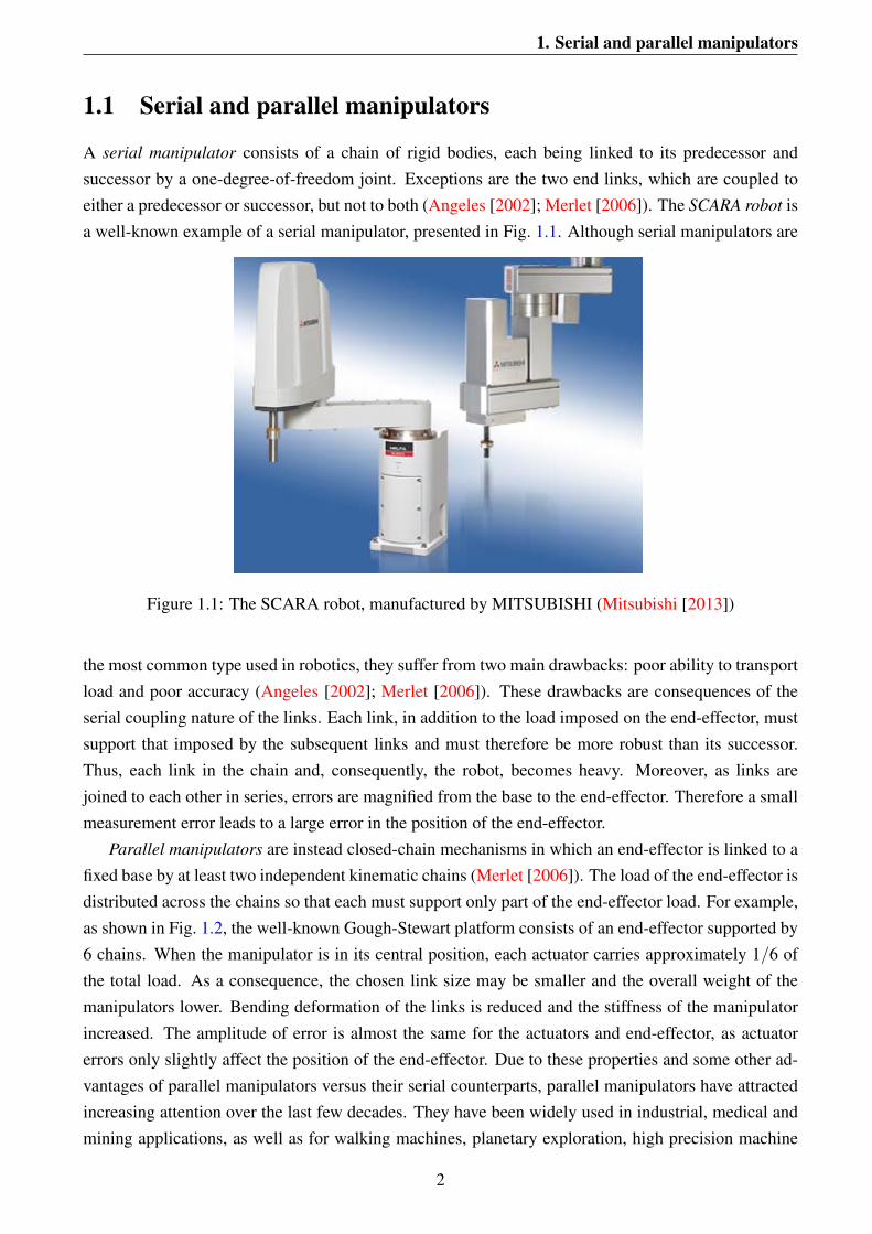
A serial manipulator consists of a chain of rigid bodies, each being linked to its predecessor andsuccessor by a one-degree-of-freedom joint. Exceptions are the two end links, which are coupled toeither a predecessor or successor, but not to both (Angeles [2002]; Merlet [2006]). The SCARA robot isa well-known example of a serial manipulator, presented in Fig. 1.1. Although serial manipulators are
Figure 1.1: The SCARA robot, manufactured by MITSUBISHI (Mitsubishi [2013])
the most common type used in robotics, they suffer from two main drawbacks: poor ability to transportload and poor accuracy (Angeles [2002]; Merlet [2006]). These drawbacks are consequences of theserial coupling nature of the links. Each link, in addition to the load imposed on the end-effector, mustsupport that imposed by the subsequent links and must therefore be more robust than its successor.Thus, each link in the chain and, consequently, the robot, becomes heavy. Moreover, as links arejoined to each other in series, errors are magnified from the base to the end-effector. Therefore a smallmeasurement error leads to a large error in the position of the end-effector.
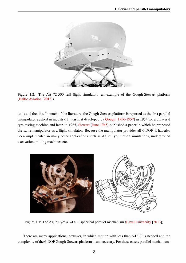
Parallel manipulators are instead closed-chain mechanisms in which an end-effector is linked to afixed base by at least two independent kinematic chains (Merlet [2006]). The load of the end-effector isdistributed across the chains so that each must support only part of the end-effector load. For example,as shown in Fig. 1.2, the well-known Gough-Stewart platform consists of an end-effector supported by6 chains. When the manipulator is in its central position, each actuator carries approximately 1/6 ofthe total load. As a consequence, the chosen link size may be smaller and the overall weight of themanipulators lower. Bending deformation of the links is reduced and the stiffness of the manipulatorincreased. The amplitude of error is almost the same for the actuators and end-effector, as actuatorerrors only slightly affect the position of the end-effector. Due to these properties and some other ad-vantages of parallel manipulators versus their serial counterparts, parallel manipulators have attractedincreasing attention over the last few decades. They have been widely used in industrial, medical andmining applications, as well as for walking machines, planetary exploration, high precision machine
2
1. Serial and parallel manipulators
Figure 1.2: The Art 72-500 full flight simulator: an example of the Gough-Stewart platform(Baltic Aviation [2013])
tools and the like. In much of the literature, the Gough-Stewart platform is reported as the first parallelmanipulator applied in industry. It was first developed by Gough [1956-1957] in 1954 for a universaltyre testing machine and later, in 1965, Stewart [June 1965] published a paper in which he proposedthe same manipulator as a flight simulator. Because the manipulator provides all 6 DOF, it has alsobeen implemented in many other applications such as Agile Eye, motion simulations, undergroundexcavation, milling machines etc.
Figure 1.3: The Agile Eye: a 3-DOF spherical parallel mechanism (Laval University [2013])
There are many applications, however, in which motion with less than 6-DOF is needed and thecomplexity of the 6-DOF Gough-Stewart platform is unnecessary. For these cases, parallel mechanisms
3
1. Serial and parallel manipulators
with limited-DOF and simpler structures are preferred.A 3-DOF spherical parallel mechanism (Fig. 1.3), introduced by Gosselin and Hamel [1994], is
such a mechanism that is used for applications like camera orienting devices and wrist motion sim-ulators. The structure of this manipulator is such that the axes of all revolute joints intersect at onecommon point that is the centre of rotation of the device. The manipulator only produces the threerotational degrees of freedom that are needed for the application.
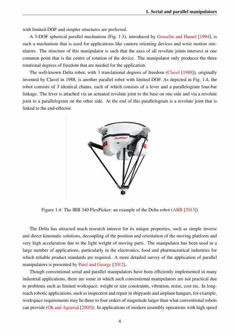
The well-known Delta robot, with 3 translational degrees of freedom (Clavel [1988]), originallyinvented by Clavel in 1988, is another parallel robot with limited DOF. As depicted in Fig. 1.4, therobot consists of 3 identical chains, each of which consists of a lever and a parallelogram four-barlinkage. The lever is attached via an actuated revolute joint to the base on one side and via a revolutejoint to a parallelogram on the other side. At the end of this parallelogram is a revolute joint that islinked to the end-effector.
Figure 1.4: The IRB 340 FlexPicker: an example of the Delta robot (ABB [2013])
The Delta has attracted much research interest for its unique properties, such as simple inverseand direct kinematic solutions, decoupling of the position and orientation of the moving platform andvery high acceleration due to the light weight of moving parts. The manipulator has been used in alarge number of applications, particularly in the electronics, food and pharmaceutical industries forwhich reliable product standards are required. A more detailed survey of the application of parallelmanipulators is presented by Patel and George [2012].
Though conventional serial and parallel manipulators have been efficiently implemented in manyindustrial applications, there are some in which such conventional manipulators are not practical dueto problems such as limited workspace, weight or size constraints, vibration, noise, cost etc. In long-reach robotic applications, such as inspection and repair in shipyards and airplane hangars, for example,workspace requirements may be three to four orders of magnitude larger than what conventional robotscan provide (Oh and Agrawal [2005]). In applications of modern assembly operations with high speed
4

1. Cable-driven parallel manipulators
robotic positioning systems, use of serial link manipulators presents problems relating to weight, vibra-tion and cost, while parallel manipulators suffer from limited workspace and high motor torque ripple(S.Kawamura et al. [1995]).
To overcome these problems, in recent years, use of cables in the place of rigid links has receivedincreasing attention. The following section presents more details on such cable-driven parallel robots.
1.2 Cable-driven parallel manipulators
Cable-driven parallel robots (CDPRs) employ cables in place of rigid body extendable legs to controlthe posture of an end-effector. In these manipulators, the pose of the end-effector is controlled appro-priately by controlling the length of the cables. Cables are usually rolled on drums attached to a baseand are actuated by rotary motor. Cable-driven parallel robots have special advantages such as a largerworkspace, reduced manufacturing and maintenance costs, ease of assembly and disassembly, hightransportability, superior modularity and ease of reconfiguration. As a consequence of the flexibilityand low weight of the cables, implementation of long cables can be easily handled. By controlling ca-ble lengths within broad ranges, a very large workspace can be accessed. This property makes CDPRsappropriate for applications in which force transmission or access over a long distance is needed. Oneof the main advantages of parallel manipulators is the reduced moving mass and inertial force. Usingcables instead of rigid links further decreases the moving mass, as the actuators do not change positionand are attached to a fixed base such that the only moving parts are the cables and end-effector. Asa consequence, a robot with higher speed and agility is obtained and the payload of the robot may beincreased (Behzadipour et al. [2003]).
Manufacturing costs of cable-driven robots are significantly lower than those of conventional ma-nipulators. A cable-driven manipulator is simple to set up with low-cost hardware. As outlined byMerlet and Daney [2010], a portable robot with a load capacity of more than 1 ton can be set up byassembling a number of low cost winches and cables.
The cable characteristic that makes the control of the end-effector challenging is its inability towithstand compression. Due to this fact, if a CDPR is intended to control a total number of end-effectordegrees of freedom (DOFs), f , at least f + 1 cables are required (Kurtz and Hayward [1995]; Mingand Higuchi [1994]; Roberts et al. [1998]). This redundancy of control actions is usually necessaryto guarantee tensile force in all cables and to prevent them from becoming slack when the imposedload on the moving platform changes. This maintains the control by cable of all degrees of freedomof the moving platform. Such systems of cable-driven parallel robots are called fully-controlled orcompletely-restrained. If the end-effector instead preserves some level of freedom once the actuatorsare locked and the cable lengths are fixed, the system is called under-constrained or incompletely-
restrained. This typically occurs when the end-effector is controlled by a number of cables, n, smallerthan f . In such a system, the platform may move and deviate from its equilibrium position. Therefore,the posture of the moving platform depends on, in addition to the length of the cables, the imposedload on the moving platform. Fully-constrained robots are attracting increasing interest in the research
5
1. Cable-driven parallel manipulators
community and, as such, a rich literature exists. In the following section, some examples of theserobots are presented.
1.2.1 Fully-constrained CDPRs
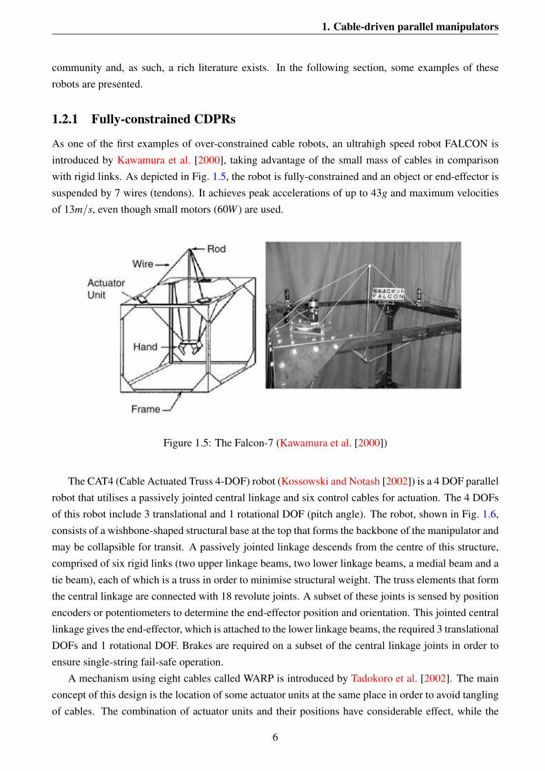
As one of the first examples of over-constrained cable robots, an ultrahigh speed robot FALCON isintroduced by Kawamura et al. [2000], taking advantage of the small mass of cables in comparisonwith rigid links. As depicted in Fig. 1.5, the robot is fully-constrained and an object or end-effector issuspended by 7 wires (tendons). It achieves peak accelerations of up to 43g and maximum velocitiesof 13m/s, even though small motors (60W ) are used.
Figure 1.5: The Falcon-7 (Kawamura et al. [2000])
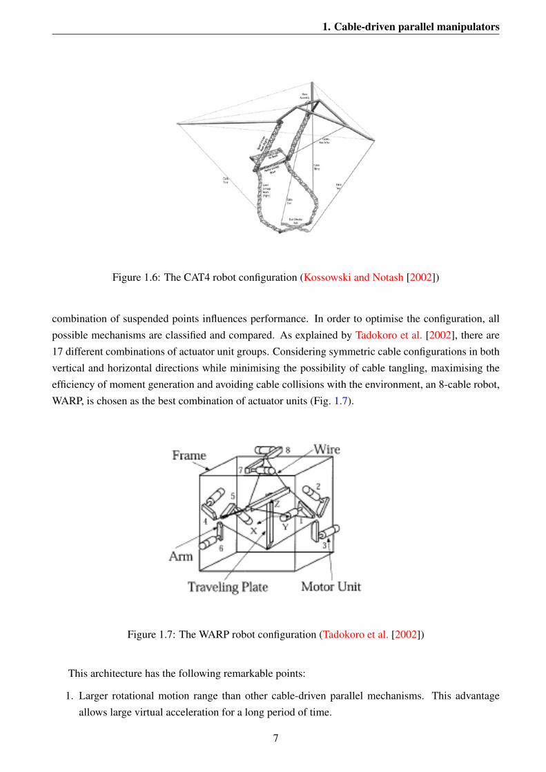
The CAT4 (Cable Actuated Truss 4-DOF) robot (Kossowski and Notash [2002]) is a 4 DOF parallelrobot that utilises a passively jointed central linkage and six control cables for actuation. The 4 DOFsof this robot include 3 translational and 1 rotational DOF (pitch angle). The robot, shown in Fig. 1.6,consists of a wishbone-shaped structural base at the top that forms the backbone of the manipulator andmay be collapsible for transit. A passively jointed linkage descends from the centre of this structure,comprised of six rigid links (two upper linkage beams, two lower linkage beams, a medial beam and atie beam), each of which is a truss in order to minimise structural weight. The truss elements that formthe central linkage are connected with 18 revolute joints. A subset of these joints is sensed by positionencoders or potentiometers to determine the end-effector position and orientation. This jointed centrallinkage gives the end-effector, which is attached to the lower linkage beams, the required 3 translationalDOFs and 1 rotational DOF. Brakes are required on a subset of the central linkage joints in order toensure single-string fail-safe operation.
A mechanism using eight cables called WARP is introduced by Tadokoro et al. [2002]. The mainconcept of this design is the location of some actuator units at the same place in order to avoid tanglingof cables. The combination of actuator units and their positions have considerable effect, while the
6
1. Cable-driven parallel manipulators
Figure 1.6: The CAT4 robot configuration (Kossowski and Notash [2002])
combination of suspended points influences performance. In order to optimise the configuration, allpossible mechanisms are classified and compared. As explained by Tadokoro et al. [2002], there are17 different combinations of actuator unit groups. Considering symmetric cable configurations in bothvertical and horizontal directions while minimising the possibility of cable tangling, maximising theefficiency of moment generation and avoiding cable collisions with the environment, an 8-cable robot,WARP, is chosen as the best combination of actuator units (Fig. 1.7).
Figure 1.7: The WARP robot configuration (Tadokoro et al. [2002])
This architecture has the following remarkable points:
1. Larger rotational motion range than other cable-driven parallel mechanisms. This advantageallows large virtual acceleration for a long period of time.
7
1. Cable-driven parallel manipulators
2. The motion platform may stay on the ground, as the bottom of the platform does not have anymechanism.
3. All walls may be used for scene projection of computer graphics, like in the CAVE virtual realitysystem.
4. Redundancy of cables improves safety in the case of failure.
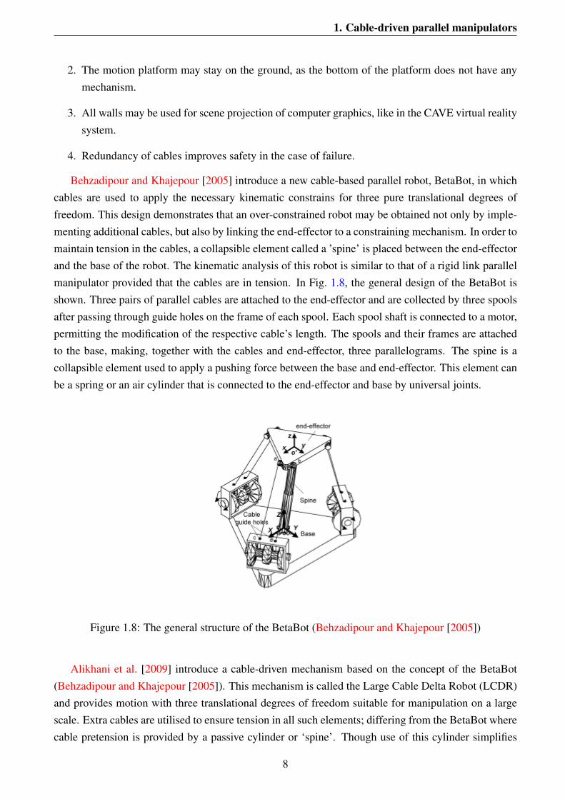
Behzadipour and Khajepour [2005] introduce a new cable-based parallel robot, BetaBot, in whichcables are used to apply the necessary kinematic constrains for three pure translational degrees offreedom. This design demonstrates that an over-constrained robot may be obtained not only by imple-menting additional cables, but also by linking the end-effector to a constraining mechanism. In order tomaintain tension in the cables, a collapsible element called a ’spine’ is placed between the end-effectorand the base of the robot. The kinematic analysis of this robot is similar to that of a rigid link parallelmanipulator provided that the cables are in tension. In Fig. 1.8, the general design of the BetaBot isshown. Three pairs of parallel cables are attached to the end-effector and are collected by three spoolsafter passing through guide holes on the frame of each spool. Each spool shaft is connected to a motor,permitting the modification of the respective cable’s length. The spools and their frames are attachedto the base, making, together with the cables and end-effector, three parallelograms. The spine is acollapsible element used to apply a pushing force between the base and end-effector. This element canbe a spring or an air cylinder that is connected to the end-effector and base by universal joints.
Figure 1.8: The general structure of the BetaBot (Behzadipour and Khajepour [2005])
Alikhani et al. [2009] introduce a cable-driven mechanism based on the concept of the BetaBot(Behzadipour and Khajepour [2005]). This mechanism is called the Large Cable Delta Robot (LCDR)and provides motion with three translational degrees of freedom suitable for manipulation on a largescale. Extra cables are utilised to ensure tension in all such elements; differing from the BetaBot wherecable pretension is provided by a passive cylinder or ‘spine’. Though use of this cylinder simplifies
8
1. Cable-driven parallel manipulators
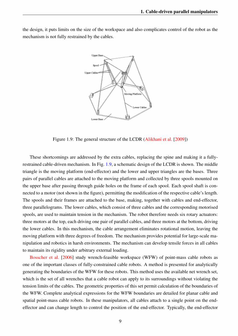
the design, it puts limits on the size of the workspace and also complicates control of the robot as themechanism is not fully restrained by the cables.
Figure 1.9: The general structure of the LCDR (Alikhani et al. [2009])
These shortcomings are addressed by the extra cables, replacing the spine and making it a fully-restrained cable-driven mechanism. In Fig. 1.9, a schematic design of the LCDR is shown. The middletriangle is the moving platform (end-effector) and the lower and upper triangles are the bases. Threepairs of parallel cables are attached to the moving platform and collected by three spools mounted onthe upper base after passing through guide holes on the frame of each spool. Each spool shaft is con-nected to a motor (not shown in the figure), permitting the modification of the respective cable’s length.The spools and their frames are attached to the base, making, together with cables and end-effector,three parallelograms. The lower cables, which consist of three cables and the corresponding motorisedspools, are used to maintain tension in the mechanism. The robot therefore needs six rotary actuators:three motors at the top, each driving one pair of parallel cables, and three motors at the bottom, drivingthe lower cables. In this mechanism, the cable arrangement eliminates rotational motion, leaving themoving platform with three degrees of freedom. The mechanism provides potential for large-scale ma-nipulation and robotics in harsh environments. The mechanism can develop tensile forces in all cablesto maintain its rigidity under arbitrary external loading.
Bosscher et al. [2006] study wrench-feasible workspace (WFW) of point-mass cable robots asone of the important classes of fully-constrained cable robots. A method is presented for analyticallygenerating the boundaries of the WFW for these robots. This method uses the available net wrench set,which is the set of all wrenches that a cable robot can apply to its surroundings without violating thetension limits of the cables. The geometric properties of this set permit calculation of the boundaries ofthe WFW. Complete analytical expressions for the WFW boundaries are detailed for planar cable andspatial point-mass cable robots. In these manipulators, all cables attach to a single point on the end-effector and can change length to control the position of the end-effector. Typically, the end-effector
9
1. Cable-driven parallel manipulators
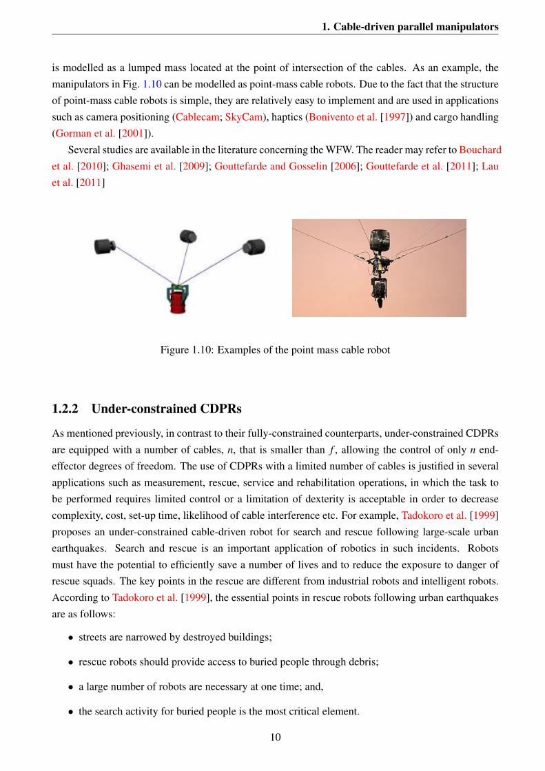
is modelled as a lumped mass located at the point of intersection of the cables. As an example, themanipulators in Fig. 1.10 can be modelled as point-mass cable robots. Due to the fact that the structureof point-mass cable robots is simple, they are relatively easy to implement and are used in applicationssuch as camera positioning (Cablecam; SkyCam), haptics (Bonivento et al. [1997]) and cargo handling(Gorman et al. [2001]).
Several studies are available in the literature concerning the WFW. The reader may refer to Bouchardet al. [2010]; Ghasemi et al. [2009]; Gouttefarde and Gosselin [2006]; Gouttefarde et al. [2011]; Lauet al. [2011]
Figure 1.10: Examples of the point mass cable robot
1.2.2 Under-constrained CDPRs
As mentioned previously, in contrast to their fully-constrained counterparts, under-constrained CDPRsare equipped with a number of cables, n, that is smaller than f , allowing the control of only n end-effector degrees of freedom. The use of CDPRs with a limited number of cables is justified in severalapplications such as measurement, rescue, service and rehabilitation operations, in which the task tobe performed requires limited control or a limitation of dexterity is acceptable in order to decreasecomplexity, cost, set-up time, likelihood of cable interference etc. For example, Tadokoro et al. [1999]proposes an under-constrained cable-driven robot for search and rescue following large-scale urbanearthquakes. Search and rescue is an important application of robotics in such incidents. Robotsmust have the potential to efficiently save a number of lives and to reduce the exposure to danger ofrescue squads. The key points in the rescue are different from industrial robots and intelligent robots.According to Tadokoro et al. [1999], the essential points in rescue robots following urban earthquakesare as follows:
• streets are narrowed by destroyed buildings;
• rescue robots should provide access to buried people through debris;
• a large number of robots are necessary at one time; and,
• the search activity for buried people is the most critical element.
10
1. Cable-driven parallel manipulators
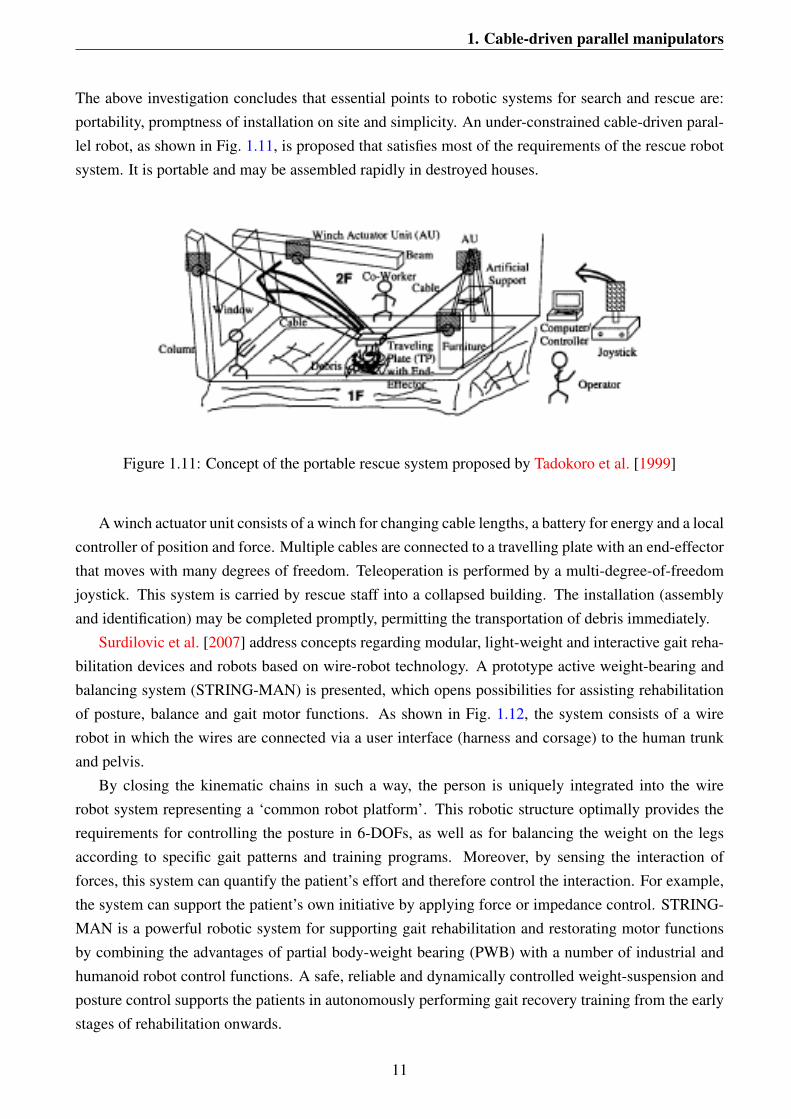
The above investigation concludes that essential points to robotic systems for search and rescue are:portability, promptness of installation on site and simplicity. An under-constrained cable-driven paral-lel robot, as shown in Fig. 1.11, is proposed that satisfies most of the requirements of the rescue robotsystem. It is portable and may be assembled rapidly in destroyed houses.
Figure 1.11: Concept of the portable rescue system proposed by Tadokoro et al. [1999]
A winch actuator unit consists of a winch for changing cable lengths, a battery for energy and a localcontroller of position and force. Multiple cables are connected to a travelling plate with an end-effectorthat moves with many degrees of freedom. Teleoperation is performed by a multi-degree-of-freedomjoystick. This system is carried by rescue staff into a collapsed building. The installation (assemblyand identification) may be completed promptly, permitting the transportation of debris immediately.
Surdilovic et al. [2007] address concepts regarding modular, light-weight and interactive gait reha-bilitation devices and robots based on wire-robot technology. A prototype active weight-bearing andbalancing system (STRING-MAN) is presented, which opens possibilities for assisting rehabilitationof posture, balance and gait motor functions. As shown in Fig. 1.12, the system consists of a wirerobot in which the wires are connected via a user interface (harness and corsage) to the human trunkand pelvis.
By closing the kinematic chains in such a way, the person is uniquely integrated into the wirerobot system representing a ‘common robot platform’. This robotic structure optimally provides therequirements for controlling the posture in 6-DOFs, as well as for balancing the weight on the legsaccording to specific gait patterns and training programs. Moreover, by sensing the interaction offorces, this system can quantify the patient’s effort and therefore control the interaction. For example,the system can support the patient’s own initiative by applying force or impedance control. STRING-MAN is a powerful robotic system for supporting gait rehabilitation and restorating motor functionsby combining the advantages of partial body-weight bearing (PWB) with a number of industrial andhumanoid robot control functions. A safe, reliable and dynamically controlled weight-suspension andposture control supports the patients in autonomously performing gait recovery training from the earlystages of rehabilitation onwards.
11
1. Cable-driven parallel manipulators
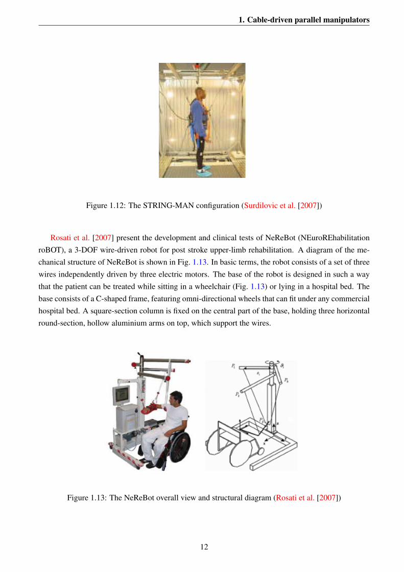
Figure 1.12: The STRING-MAN configuration (Surdilovic et al. [2007])
Rosati et al. [2007] present the development and clinical tests of NeReBot (NEuroREhabilitationroBOT), a 3-DOF wire-driven robot for post stroke upper-limb rehabilitation. A diagram of the me-chanical structure of NeReBot is shown in Fig. 1.13. In basic terms, the robot consists of a set of threewires independently driven by three electric motors. The base of the robot is designed in such a waythat the patient can be treated while sitting in a wheelchair (Fig. 1.13) or lying in a hospital bed. Thebase consists of a C-shaped frame, featuring omni-directional wheels that can fit under any commercialhospital bed. A square-section column is fixed on the central part of the base, holding three horizontalround-section, hollow aluminium arms on top, which support the wires.
Figure 1.13: The NeReBot overall view and structural diagram (Rosati et al. [2007])
12
1. Cable-driven parallel manipulators
The free ends of each wire are fastened to the patient’s arm by means of a special splint. Bycontrolling wire length, rehabilitation treatment (based on the passive or active spatial motion of thelimb) can be delivered over a large working space. The arm trajectory is set by the therapist througha very simple teach-by-showing procedure, enabling most common ‘hands on’ therapy exercises to bereproduced by the robot. Compared to other rehabilitation robots, NeReBot offers advantages due to itslow-cost mechanical structure, intrinsically safe treatment thanks to the use of wires, good acceptanceby patients who do not feel constrained by an ‘industrial-like’ robot, transportability as it can easily beplaced beside a hospital bed and/or wheelchair and good trade-off between low number of DOF andspatial performance. These features, along with the very encouraging results of the first clinical trials,make the NeReBot a good candidate for adoption in the rehabilitation of subacute stroke survivors.
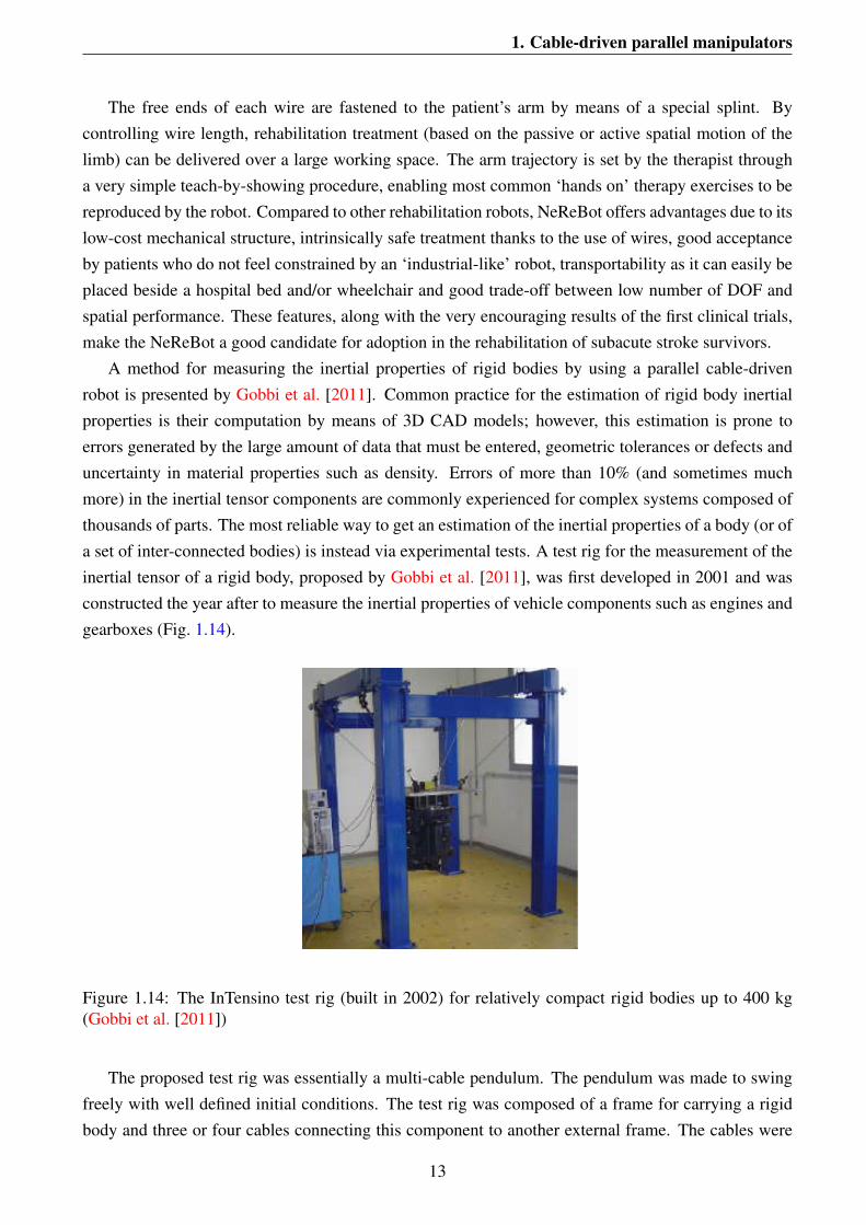
A method for measuring the inertial properties of rigid bodies by using a parallel cable-drivenrobot is presented by Gobbi et al. [2011]. Common practice for the estimation of rigid body inertialproperties is their computation by means of 3D CAD models; however, this estimation is prone toerrors generated by the large amount of data that must be entered, geometric tolerances or defects anduncertainty in material properties such as density. Errors of more than 10% (and sometimes muchmore) in the inertial tensor components are commonly experienced for complex systems composed ofthousands of parts. The most reliable way to get an estimation of the inertial properties of a body (or ofa set of inter-connected bodies) is instead via experimental tests. A test rig for the measurement of theinertial tensor of a rigid body, proposed by Gobbi et al. [2011], was first developed in 2001 and wasconstructed the year after to measure the inertial properties of vehicle components such as engines andgearboxes (Fig. 1.14).
Figure 1.14: The InTensino test rig (built in 2002) for relatively compact rigid bodies up to 400 kg(Gobbi et al. [2011])
The proposed test rig was essentially a multi-cable pendulum. The pendulum was made to swingfreely with well defined initial conditions. The test rig was composed of a frame for carrying a rigidbody and three or four cables connecting this component to another external frame. The cables were
13
1. Cable-driven parallel manipulators
connected at both ends by low-friction spherical joints, each comprising a Hook’s joint fitted withroller bearings and an axial bearing. Given a rigid body with a particular mass, the method allowsidentification and measurement of the centre of gravity and the inertial tensor with a single test. Theproposed technique is based on the analysis of the free motion of the multi-cable pendulum to whichthe body under consideration is connected. The motion of the pendulum and the forces acting on thesystem are recorded and the inertial properties identified by means of a mathematical procedure basedon a least squares estimation. The natural frequencies of the pendulum and the accelerations involvedare quite low, making this method suitable for many practical applications.
1.2.2.1 The challenges in studying displacement of under-constrained CDPRs and the objectiveof the thesis
Compared to fully-constrained manipulators, under-constrained CDPRs have seen little attention in theliterature and the study of these types of robots is still an open field. For instance, analysis of displace-ment as a first step in the study of robots is ongoing for the case of under-constrained CDPRs. Themajor challenge in the displacement study of under-constrained CDPRs consists of the intrinsic cou-pling between kinematics and statics (or dynamics). When a fully-constrained CDPR operates in theportion of its workspace in which the required set of output wrenches is guaranteed with purely tensilecable forces, the posture of the end-effector is determined in a purely geometric way by assigning ca-ble lengths. Conversely, for an under-constrained CDPR, when the actuators are locked and the cablelengths are assigned, the end-effector is still able to move, so the actual configuration is determined bythe applied forces. As a consequence, the end-effector posture depends on both the cable lengths andequilibrium equations. Moreover, as the end-effector pose depends on the applied load, it may changedue to external disturbances. As such, these factors are fundamental to the investigation of equilibriumstability. The necessity of simultaneously dealing with kinematics and statics increases the complexityof position problems aimed at determining the overall robot configuration when a set of n variables isassigned. The solution to these problems is significantly more difficult than analogous tasks concern-ing rigid-link parallel manipulators. In the literature, some procedures have been presented to solvethe following problems.
Ghasemi et al. [2010] suggest the use of neural networks to solve the system of polynomial equa-tions associated with forward displacement analysis of under-constrained cable-driven parallel manip-ulators. According to this scheme, the neural network is trained by solving the corresponding inversedisplacement analysis, which is much easier than the original problem, over a large set of poses. Theresulting neural network may provide a good approximation of the forward displacement analysis inmany cases; however, it does not guarantee the convergence to an equilibrium pose in general.
Michael et al. [2011] propose a solution to the case of n = 2 cables (i.e. the planar case). Thissolution is obtained by finding the equilibrium points on the coupler curve of the analogous planarfour-bar linkage. In the same work, the authors adopt an energetic approach to the case of n = 3, usingthe fact that an equilibrium pose corresponds to a minimum in the potential energy. This leads to anon-convex optimisation problem, whose optima are obtained by varying the initial guess of a local
14
1. Cable-driven parallel manipulators
optimisation procedure. Fink et al. [2011] instead relax the same formulated optimisation problem intoa convex optimisation problem. The optimum objective value of the relaxed problem may be regardedas a lower bound on the optimum value of the original problem. Furthermore, the authors providegeometric conditions under which the lower bound is guaranteed as tight; that is, under which theoptima of the relaxed and original problem coincide.
In a parallel effort, Jiang and Kumar [2010] were able to compute all stable equilibrium poses fora class of special cases in three-dimensional space. A particular geometry is a member of this class if:
• the cable attachment points on the rigid body are located at the vertices of a regular polygon;
• the rigid-body centre of mass is at the centroid of the said polygon;
• the fixed cable attachment points (i.e. those on the supporting frame) form a regular polygonwith the same planes of symmetry as the rigid-body polygon;
• this fixed polygon is perpendicular to gravity (i.e. lies in a horizontal plane).
These constraints allow the decomposition of the spatial problem into several planar problems, whichmay be solved by computing the stationary points on the coupler curve of the equivalent four-barlinkage.
Collard and Cardou [2013], proceeding very much like Fink et al. [2011], relax the energy min-imisation problem. The relaxation, however, is different and the lower bound provided by it is castin a branch-and-bound algorithm, which allows the computation of a global optimum to the energy-minimisation problem. This global optimum corresponds to the lowest equilibrium pose and provides atight lower bound on the height of the rigid-body centre of gravity, a piece of information that is usefulfor guaranteeing no collisions while moving a cable-suspended object above possible obstacles. Theproposed method can be applied to problems with large numbers of cables, which sets it apart from theother solutions.
In light of this brief overview, it may be noted that most studies related to under-constrained CD-PRs rely on purely local numerical solution strategies; whereas, no adequate consideration is given toconceiving static geometric models capable of providing broader solution strategies, tailored to obtainthe complete solution sets of the nonlinear equations governing the problem.
In the present thesis, a methodology is proposed for the kinematic, static and stability analysisof general under-constrained n-n CDPRs, namely parallel robots in which a fixed base and a mobileplatform are inter-connected by n cables, with n≤ 6, and the anchor points on the base and the platformare generally distinct. The procedure aims at effectively solving the inverse and direct static geometricproblems; that is, at finding the overall robot configuration and cable tensions when a set of n platformposture coordinates or n cable lengths are assigned, under the assumption that a constant force isapplied on the platform, that the cables are inextensible and massless, and that interference problemsare not present.
15
Chapter 2
Mathematical development for solvingsystems of polynomials
Due to the high complexity of systems of polynomials that arise in displacement analysis of under-constrained cable-driven parallel robots, a suitable mathematical framework for their resolution is re-quired. Two approaches are often used in the context of kinematics: elimination methods based oncomputational algebraic geometry and continuation homotopy. The former is a geometric manifesta-tion of the solutions of systems of polynomial equations (Cox et al. [2005]). It provides a powerfultheoretical technique for studying the qualitative and quantitative features of the solution sets. Theapplication of algebraic geometry to kinematic analysis is more natural to a global understanding ofthe entire solution set, as opposed to finding only some of the solutions (Masouleh [2010]).
On the other hand, the elimination method may be time consuming and, as such, a numerical pro-cedure is required as a robust and fast method for computing the complete set of equations governingthe problem for a given set of parameters. To this end, polynomial homotopy continuation may beused. The procedure has the advantage that very little symbolic information must be extracted froma polynomial system to proceed. It often suffices, for example, to simply know the degree of eachpolynomial, which is easily obtained without a full expansion into terms.
Although the upper bound on the number of solutions of a system of polynomials in the complexfield may be known and all solutions computed by the two aforementioned methods, there may notbe any available information about the upper bound on the number of real solutions that a family ofsystems of polynomials may exhibit. In fact, since there may be roots in the solution set that alwaysremain complex, it may result that the number of real solutions is smaller than the number of complexones. The upper bound on the number of real solutions has significant importance in the kinematicanalysis of robots, as it indicates the maximum number of assembly modes that a robot may admit.Thus, finding a set of robot parameters admitting the maximum number of real solutions is a classicquestion in robot kinematics. For example, although it was known that the direct kinematic problem ofthe Gough-Stewart platform admitted 40 solutions, a set of the robot parameters with such a numberof real solutions was unknown for years until Dietmaier [1998] proposed an algorithm capable ofproviding them. In this context, the same algorithm is adapted to finding a set of robot parameters with
16

2. Computational algebraic geometry
the maximum number of real assembly modes to the problems emerging in displacement analysis ofCDPRs.
Accordingly, in the first part of this chapter, the concept of computational algebraic geometryis introduced and the required algorithms presented for solving the systems of polynomials arising indisplacement analysis of under-constrained CDPRs. In the subsequent part, the homotopy continuationmethod is presented briefly with its various features and some required terminology. In the final sectionof this chapter, the Dietmaier algorithm is also briefly discussed.
2.1 Computational algebraic geometry
The origin of algebraic geometry dates back to Descartes’ introduction of coordinates to describepoints in Euclidean space and the idea of describing curves and surfaces by algebraic equations. Overthe long history of the subject, both powerful general theories and detailed knowledge of many specificexamples have been developed (Cox et al. [2005]). Recently, the advent of computer algebra systemshas made it possible to implement many theories of algebraic geometry relating to robotics using com-putational algorithms (Brunnthaler [2006]; Masouleh [2010]; Pfurner [2006]). As will be seen in thefollowing chapters, similar problems emerging in displacement analysis of under-constrained CDPRsare analysed using these concepts. Before discussing computational algebraic geometry, some impor-tant terminology must be provided. In particular, an introduction to the ideals of the polynomial ringK[x1, . . . , xn] will be provided in the following section, followed by an explanation of the total orderof monomials and an introduction to the Groebner basis as one of the powerful elimination strategiesfor solving systems of polynomials. There are several software packages that offer the Groebner basistechnique for solving systems of polynomials. In the present thesis, Maple (Maplesoft) is mainly usedto implement the Groebner base technique.
2.1.1 Polynomials and affine varieties
A field is a set where addition, subtraction, multiplication and division are defined with their usualproperties. Standard examples are the real numbers and complex numbers; whereas, integers are not afield since division fails. Due to the importance of both real and complex solutions to the problem athand, most of the computation will be performed in the complex field K = C. On the other hand, forsimplification of computation at many points, the field of rational numbers K=Q will be used.
A monomial in x1, . . . , xn is a product of the form:
xα11 · x
α22 . . .xαn
n (2.1)
where all exponents α1, . . . , αn are nonnegative integers. The total degree of this monomial is the sumα1 + . . .+αn. The notation for monomials is simplified by setting α = (α1, . . . , αn) as a n-tuple of
17

2. Computational algebraic geometry
nonnegative integers and, correspondingly:
xα = xα11 · x
α22 . . .xαn
n (2.2)
Knowing the definition of a monomial, a polynomial is defined as follows:A polynomial, f in x1, . . . , xn with coefficients in K, is a finite linear combination (with coefficients
in K) of monomials. It can be written in the form:
f = ∑α
aαxα (2.3)
where the sum is over a finite number of n-tuples α = (α1, . . . , αn). The set of all polynomials inX = x1, . . . , xn with coefficients in K is denoted K[X]. When dealing with a polynomial such as f =
∑α aαxα , aα is called the coefficient of the monomial xα . If aα 6= 0, then aαxα is a term of f and thetotal degree of f , denoted deg( f ), is the maximum |α| where the coefficient aα is nonzero.
According to a special property of polynomials over the field of complex numbers where everynon-constant polynomial f ∈K has a root in K, the concept of affine variety is defined as follows.
Let f1, . . . , fs be polynomials in K[X], then V ( f1, . . . , fs), called the affine variety defined byf1, . . . , fs, is:
V ( f1, . . . , fs) = {(x1, . . . , xn) ∈Kn : fi(x1, . . . , xn) = 0, 1≤ i≤ s} (2.4)
An affine variety, V ( f1, . . . , fs) ⊂ Kn, is the set of all solutions of the system of equations f1(x1,. . . , xn) = . . . = fs(x1, . . . , xn) = 0. In the present work, the letters V ,W etcetera, where not otherwisestated, are used to denote affine varieties.
2.1.2 Ideals
Ideals define the basic algebraic objects that are used in the present work. A subset 〈I〉 ∈ K[X ] is anideal if it satisfies:
• 0 ∈ 〈I〉
• If f , g ∈ 〈I〉, then f +g ∈ 〈I〉
• If f ∈ 〈I〉 and h ∈K[X], then h f ∈ 〈I〉
Given a collection of polynomials, I = { f1, . . . , fs} ∈ K[X], all polynomials that may be built upfrom these by multiplication or sums of arbitrary polynomials are denoted as:
〈I〉= 〈 f1, . . . , fs〉= {p1 f1 + . . .+ ps fs : pi ∈K[X] f or i = 1, . . . , s} (2.5)
From this definition it can be proven that 〈I〉 is an ideal. 〈I〉 is called the ideal generated by I =
{ f1, . . . , fs}.
18
2. Computational algebraic geometry
2.1.3 Monomial orders and polynomial division
One of the key elements for all operations relating to algorithms for solving a system of polynomialsis ordering of terms. This will be used regularly in the present work. A monomial order on K[X] isany relation > on the set of monomials xα in K[X] satisfying:
1. > is a total (linear) ordering relation
2. > is compatible with multiplication in K[X]; that is, if xα > xβ and xγ is any monomial, thenxαxγ = xα+γ > xβ+γ = xβ xγ
3. > is well-ordering; that is, every nonempty collection of monomials has a smallest element under>.
According to this definition, there are many ways to define monomial orders. The most important ofthese, in the present study, are as follows.
Lexicographic order (lex) first compares exponents of x1 and, in the case of equality, comparesexponents of x2 and so forth. Therefore, if xα and xβ are monomials in K[X], xα >lex xβ if, in thedifference α−β ∈ Zn, the leftmost nonzero entry is positive.
Graded lexicographic order (grlex) first compares the sum of all exponents and, in the caseof equality, applies lexicographic ordering. In this case, xα >grlex xβ if ∑
ni=1αi > ∑
ni=1βi; or if
∑n
i=1αi = ∑n
i=1βi, then xα >lex xβ .Graded reverse lexicographic order (grevlex) first compares the total degree then compares ex-
ponents of the last indeterminate xn, reversing the result. In the case of equality, a similar comparisonof xn−1 is performed and so forth ending in x1. Accordingly, xα >grevlex xβ if ∑
ni=1αi > ∑
ni=1βi or if
∑n
i=1αi = ∑n
i=1βi and the rightmost nonzero entry is negative in the difference α−β ∈ Zn.There are many other monomial orders besides the ones considered here; however, the aforemen-
tioned orders will be used at many points in the present work. It will be shown that, while grevlexis almost always much easier for performing some computations, there are many cases in which cal-culations based on lex or grlex must be performed. It will also be shown that by implementing thecomputations in certain orders and combinations they may be performed more efficiently.
For a particular monomial order >, the terms are considered to be of the form cαxα . The leadingterm of f (with respect to >) is then the product cαxα , where xα is the largest monomial appearing in f
in the ordering >. The notation LT>( f ) is used for the leading term, or simply LT ( f ) where it is clearwhich monomial order is being used. Furthermore, if LT ( f ) = cαxα , then LC( f ) = cα is the leadingcoefficient of f and LM( f ) = xα is the leading monomial. One of the first uses of monomial orders isin the division algorithm, defined as follows:
Taking any monomial order > in K[X] and letting I = { f1, . . . , fs} be a set of polynomials in K[X],then every f ∈K[X] can be written as:
f = a1 f1 + . . .+as fs + r (2.6)
19
2. Computational algebraic geometry
Term r is a remainder of f on division by I, with either r = 0 or r being a linear combination ofmonomials, none of which is divisible by any of LT>( f1), . . . , LT>( fs).
According to this definition of division, reordering I or changing the monomial order can producedifferent ai and r in some cases.
2.1.4 Groebner bases
Since a division algorithm in K[X] has been obtained, one would expect the possibility to determine ifa given f ∈ K[X] is a member of an ideal, 〈I〉 = 〈 f1, . . . , fs〉, by computing its remainder on division.From Eq.(2.6) it follows that, if r = 0 on dividing by I = { f1, . . . , fs}, then f = a1 f1 + . . .+ as fs andf ∈ 〈I〉 = 〈 f1 . . . fs〉. It can be shown, however, that r = 0 is not guaranteed for every f ∈ 〈I〉 if anarbitrary basis I is used for 〈I〉. To produce zero remainders for all elements of I upon division, aGroebner base as a basis of the ideal is defined as follows. The key idea is that once a monomialordering is chosen, each f ∈K[X] has a unique leading term, LT ( f ).
Monomial ideal: An ideal 〈I〉 in K[X] is a monomial ideal if it is generated by a collection (notnecessarily finite) of monomials. Let 〈I〉 be an ideal in K[X], other than 〈0〉. Let LT (I) denote theset {LT ( fi), fi ∈ 〈I〉} and 〈LT (I)〉 denote the ideal generated by the elements of LT (I). 〈LT ( f1), . . . ,LT ( ft)〉 and 〈LT (I)〉 can be different ideals. In general, 〈LT ( f1), . . . , LT ( ft)〉 ∈ 〈LT (I)〉.
Hilbert basis theorem: Every ideal 〈I〉 in K[X] has a finite generating set. That is, I = {g1, . . . , gr}for some g1, . . . , gr ∈ I.
Groebner bases: For a fixed monomial order > on K[X] and 〈I〉 ⊂ K[X] as an ideal, a Groebnerbasis G>[I] of 〈I〉 (with respect to >) is a finite collection of polynomials G = {g1, . . . , gt} ⊂ 〈I〉 withthe property that for every nonzero f ⊂ 〈I〉, LT ( f ) is divisible by LT (gi) for some i.
It can be proven that the remainder, r, on division of a generic polynomial f ∈K[X] by a Groebnerbasis, G>[I] of 〈I〉, is uniquely dependent on the choice of monomial order only and not on the waythe division is performed. The remainder, r, is called the normal form of f . Indeed, uniqueness ofremainders is the main characterisation of Groebner bases. In other words, all of the monomials in r
are in the normal set of 〈I〉, which is a collection of all monomials not in 〈LT (gi)〉. The normal set,N[I], contains all monomials that may appear in the remainder of all polynomials on division by G>[I];defined as follows:
Normal set: Let 〈I〉 be in K[X] and G>[I] be its Groebner basis (with respect to >); then:
N[I] = {xα | xα /∈ 〈LT (G>[I])〉} (2.7)
is the normal set (of I with respect to >).As a consequence of the Hilbert basis theorem it can be be stated that every ideal 〈I〉 in K[X] other
than 〈0〉 has a Groebner basis. Furthermore, any Groebner basis G>[I] of 〈I〉 is a basis of 〈I〉.From the definition of a Groebner basis, stated above, one may conclude that if G>[I] is a Groebner
basis of 〈I〉, then the normal set of 〈I〉 is just the normal set of the leading monomials of G>[I].Useful for many purposes relating to Groebner bases is an algorithm developed by Buchberger that
20
2. Computational algebraic geometry
takes an arbitrary generating set { f1, . . . , fs} ⊂ 〈I〉 and produces a Groebner basis G>[I] of 〈I〉 fromit. This algorithm works by forming new elements of I using expressions guaranteed to cancel leadingterms and uncover other possible leading terms. It was developed from two basic tools, the reductionor division process and the critical pairs or S-polynomials.
Let f , g in K[X] be non-zero polynomials.
1. If deg( f ) =α and deg(g) = β , then γ is (γ1, . . . , γn), where γi =max(αi, βi) for each i. Term xγ iscalled the least common multiple of LM( f ) and LM(g), noting that xγ = LCM(LM( f ), LM(g)).
2. The S-polynomial of f and g is:
S( f , g) =xγ
LT ( f )f − xγ
LT ( f )g (2.8)
An S-polynomial, S( f , g), is designed to produce cancellation of leading terms. Using the S-polynomialsanother characterisation of Groebner bases is obtained, which is, from an algorithmic point of view,more useful than the definition:
Let 〈I〉 be a polynomial ideal. Then a basis G = {g1, . . . , gs} for 〈I〉 is a Groebner basis G>[I] of〈I〉 if and only if, for all pairs i 6= j, the remainder of the division of S(gi, g j) by G>[I] (listed in someorder) is zero.
More details on the algorithm and how to compute the Groebner bases can be found in Cox et al.[2007]. There are many computer algebra systems in which Buchberger’s algorithm is installed; how-ever, as the algorithm may need large amounts of storage and take many steps, the actual Groebnerbasis computation may fail in many cases.
2.1.5 Solving polynomial systems based on Groebner bases
How to solve a system of equations based on the knowledge of Groebner bases will be outlined in thepresent section.
2.1.5.1 Elimination ordering
The most straightforward procedure for solving a system of polynomials, I, is based on the eliminationproperties of Groebner bases computed according to some elimination monomial order such as theLexicographic order. For this technique, the main tools are the Elimination and Extension Theorems.If Xl = [x1, . . . , xl] is a list of l variables in X = [x1, . . . , xl−1, xl , xl+1, . . . , xn] and X\Xl is the (ordered)relative complement of Xl in X, a monomial order >l on K[X] is of l-elimination type provided thatany monomial involving a variable in Xl is greater than any monomial in K[X\Xl]. If G>l[I] is aGroebner basis of 〈I〉 with respect to >l , then G>l[I]∩K[X\Xl] is a basis of the lth elimination ideal,〈Il〉 := 〈I〉∩K[X\Xl] (Cox et al. [2007]). The elements of Il are actually linear combinations of I =
{ f1, . . . , fn}, with polynomial coefficients that eliminate x1, . . . , xl from the equations f1 = . . .= fn = 0.As 〈I〉 comprises n variables, the polynomials of 〈I1〉 contain n− 1 variables, the polynomials of 〈I2〉
21

2. Computational algebraic geometry
n− 2, and so on. 〈In−1〉 comprises a single variable and, thus, contains a scalar multiple of the least-degree polynomial of 〈I〉 in that variable. The implemented l-elimination monomial order inducesgrevlex orders on both K[Xl] and K[X\Xl].
Considering a point (al+1, . . . , an) ∈V (Il)⊂Kn−l as a partial solution, it can be proven that, in K,this partial solution may be extended to (al , al+1, . . . , an) in V (Il−1). The Elimination theorem showsthat a lex Groebner basis, G>, successively eliminates more and more variables. Accordingly, to find allsolutions of the system one may start with the polynomials in G[I] with the fewest variables, solve themand then try to extend these partial solutions to those of the whole system by applying the extensiontheorem one variable at a time. A lex Groebner basis, however, tends to be very large and thus, evenfor problems of moderate complexity, they have little chance of actually being computed. Conversely,the graded reverse lexicographic order produces bases that are endowed with no particular structuresuitable for elimination purposes; however, it provides more efficient calculations. In this perspective,the FGLM algorithm (Faugere et al. [1993]), which converts a Groebner basis from one monomialorder to another, may be called upon to compute elimination ideals of the type 〈I〉∩K[X\Xl], startingfrom a Groebner basis G[I] computed with respect to a grevlex monomial ordering. For example, onecan derive G>l[I] from G[I], for some l. Once G>l[I] is known, one may extract the subset of allpolynomials of G>l[I] that comprise variables in X\Xl only. These polynomials will form a Groebnerbasis of 〈Il〉 with respect to grevlex(X\Xl). By computing elimination ideals via the FGLM algorithm,a least-degree polynomial in one variable may be obtained.
2.1.5.2 Eigenproblem method
In contrast to the discussion in the previous section, where elimination was necessary to obtain aunivariate polynomial, the eigenproblem method only needs some Groebner basis, not necessarily anelimination order. In this section, a simple explanation of the method by Sommese and Wampler [2005]is provided.
Consider an ideal 〈I〉 in K[X] with Groebner basis G>l[I]. Let λ be any linear combination:
λ = c0 + c1x1 + . . .+ cnxn (2.9)
for given constants c0, . . . , cn. Consider the normal set, N[I]:
N[I] = [t1, . . . , tn]T (2.10)
Let the polynomial Pi(X) = λ ti for some i and consider a solution of 〈I〉 as X∗.Since f (X∗) = 0 for any f ∈ 〈I〉, any multiple of a polynomial in the ideal 〈I〉 can be added to
Pi without changing the value of Pi(X∗). This implies that, if ri is the remainder of Pi on division byG[I], then ri(X∗) = Pi(X∗) = λ ti. But ri(X) is a sum of terms in the normal set, so it can be writtenas ri = [ai1 . . .aik]N[I]. The entries ai j are the constant coefficients in the formulae for the remaindersri, i = 1, . . . , k. Since ri−λ ti belongs to 〈I〉, it must vanish on V [I]. By assembling all equations of this
22
2. Computational algebraic geometry
kind that may be obtained for t1, . . . , tn, one has:
(A[I, λ ]−λ I)N[I] = 0 (2.11)
where A[I, λ ] = [aik] is an n×n numeric matrix called the multiplication matrix for λ and I is the n×n
identity matrix. Therefore, by computing remainders using the Groebner basis, an eigenvalue problemis derived. For each eigenvector, [N], a unique solution can be obtained, as it is either in N[I] or is aleading monomial of G. In the latter case, the solution must simply be evaluated using the Groebnerbasis element for which it is the leading monomial.
2.1.5.3 Dialytic elimination
As discussed in Section 2.1.5.1, Groebner bases with respect to some elimination monomial orders arerequired in order to eliminate unknowns. In theory, by computing elimination ideals via the FGLM al-gorithm, a least-degree polynomial in one variable may be calculated. In practice, however, computing〈Jl〉 is very demanding in terms of both computation time and memory usage, and the procedure maylikely fail. A more efficient alternative that will be implemented in the present work is provided by theGroebner-Sylvester hybrid approach, proposed by Dhingra et al. [2000]. Let 〈I〉 be an ideal of poly-nomials in K[X] and G>l[I] be the corresponding Groebner base with respect to an ordering >l . WithGroebner base G known, it may be possible to construct Sylvester’s matrix using all the polynomialsin G[I] or a subset, H[I], of G[I]. Accordingly, a variable xl ∈ X may exist such that the number ofpolynomials in G[I] or H[I] equals the number of monomials in the variables of X−xl appearing in thepolynomials. The subset H[I] of G[I] may even be derived from the Groebner basis of any eliminationideal of 〈Il〉. Using the FGLM algorithm, a subset of the original unknowns is eliminated, thus com-puting G[Jl] for some l. The elimination process is then completed by applying Dialytic elimination tothe polynomials of G[Jl]. More specifically, if either the entire set of polynomials in G[Il] or a subset,H[I], of G[Il] is used to set up the Sylvester’s matrix, there may exist q polynomials hi, i = 1 . . .q interms of {x1, . . . , xn} ⊂ X. If each hi ∈K[x1, . . . , xn] is expressed as:
hi = ∑j
a′i jm′j, a′i j ∈K[xl], m′j ∈K[x1, . . . , xl−1, xl+1, . . . , xn] (2.12)
the number of monomials, m′j, in H = {h1, . . . , hq}, including 1, may be equal to q (the number ofpolynomials in H). Considering H as a square system of homogeneous linear polynomials in theunknown monomials m′1 = 1, m′2, . . . , m′q, the matrix form may be derived as:
h1...
hq
=
[q×q
a′i j ∈K[xl]
]︸ ︷︷ ︸
S
m′q...
m′2m′1 = 1
︸ ︷︷ ︸
E
(2.13)
23

2. Computational algebraic geometry
where S is a q× q Sylvester’s (coefficient) matrix polynomial in xl and E is a q-dimensional vectorcomprising all monomials in G[Il] having variables in X− xl . Letting the determinant of Sylvester’smatrix, S(xl), vanish yields a spurious-root-free univariate least-degree polynomial in xl . In this al-gorithm, the key factor in computing the univariate polynomial efficiently is reaching a compromisebetween the time required to compute the lth elimination ideal and the size of the Sylvester matrix thatis obtained from the corresponding G[Il].
2.2 Homotopy Continuation
General homotopy continuation consists of a start system with known solutions, a schedule for trans-forming the start system into a target system and a method for tracking solution paths as the trans-formation proceeds. Before discussion of each step, some terminology necessary for understandingpolynomial continuation must be introduced.
1. Total degree of polynomial system: The total degree of a system of n polynomial equations forn unknowns is the product ∏
nj=1d j, where d j is the degree of the jth polynomial.
2. Projective Space:
N-dimensional complex projective space, denoted PN , is the space of complex lines through theorigin in CN+1. Points in PN are given by (N + 1)-tuples of complex numbers [z0, . . . , zN ], notall zero, with the equivalence relation given by [z0, . . . , zN ]v [z0
′, . . . , zN′] if and only if there is
a nonzero complex number λ such that z j′ = λ z j for j = 0, . . . , N.
This definition makes sense, because a line through the origin in CN+1 is a set of the form:
{(λ z0, . . . , λ zN) ∈ CN+1 | λ ∈ C} (2.14)
with not all zi zero. The zi occurring within the brackets, [z0, . . . , zN ], are called homogeneouscoordinates, even though they are not coordinates on PN , but rather coordinates on CN+1.
3. Multi-homogeneous polynomial:
A polynomial system F of n equations, f1, f2, . . . fn in the n unknowns, z1, z2, . . .zn is ho-mogenized by partitioning the variables into m collections, denoted Z1, . . . , Zm where Z j =
{z1 j, . . . , zk j j}. So that Z j contains k j variables and ∑m
j=1k j = n. Now choosing homogeneousvariables z0 j for j = 1 to m, and including these in Z j gives Z j = {z0 j, z1 j, . . . , zk j j}. Remindingthe substitution zi j← zi j/z0 j for i = 1 to k j and j = 1 to m, generates a system F ′ of n equationsin n+m unknowns (after we clear the denominators of powers of the z0 j).
Such a system is called m-homogeneous, understood to include the case of 1-homogeneous. Itis said that a multi-homogeneous system, F , is compatible with the multi-projective space, X , ifthe dimensions n1, . . . , nm match.
24
2. Computational algebraic geometry
As a further explanation of multi-homogeneous polynomials, the following example by Wampleret al. [1990] is provided. Consider the system:
x2−1 = 0
xy−1 = 0(2.15)
which is the intersection of two vertical lines, x = ±1, with a hyperbola. The system has atotal degree of 4, but only two finite solutions: (x, y) = (1, 1) and (−1, − 1). Introducing thehomogeneous variable w via the substitutions x← x/w, y← y/w, we obtain:
x2−w2 = 0
xy−w2 = 0(2.16)
which, in addition to the original solutions (w, x, y) = (1, 1, 1), (1, − 1, − 1), has a solution atinfinity (0, 0, 1) of multiplicity two. Now, consider what happens if two homogeneous variablesare introduced via the substitutions x← x/w1, y← y/w2, creating the system:
x2−w21 = 0
xy−w1w2 = 0(2.17)
Disallowing any solution where (w1, x) = (0, 0) or (w2, y) = (0, 0), one may confirm that the onlysolutions are the original finite solutions: (w1, x;w2, y) = (1, 1;1, 1) and (1, − 1;1, − 1). Thisis due to the different treatment of infinity with the introduction of more than one homogeneousvariable. The system is called “2-homogeneous” because there are two homogeneous variables.Thus, it can be seen that the use of multiple homogeneous variables can sometimes reduce thenumber of solutions at infinity, which will reduce the computational load when calculating allsolutions of the system.
4. Bezout’s Theorem:
In a multi-homogeneous system of polynomials, the multi-homogeneous degree of equation l
with respect to group j, d jl , is computed as the sum of the variable exponents of group j
in any term from polynomial l. Bezout’s theorem states that the Bezout number of a multi-homogeneous system of polynomial equations in complex projective space is equal to the coef-ficient of ∏
mj=1α j
k j in the product
∏nl=1(∑
j=1
md jlα j) (2.18)
Applying this formula to equation Eq. (2.17), it is found that the coefficient of α1α2 in 2α1(α1+
α2) is 2, as expected. It can be shown that for a 1-homogeneous system, this formula yields thetotal degree.
25

2. Computational algebraic geometry
Δt
predict
correctY(t)
t
Figure 2.1: Schematic of path tracking
2.2.1 Basic polynomial continuation
Basic polynomial continuation is a path-tracking technique that transforms a start system of polynomialequations with known solutions to a target system whose solutions must be found (Sommese andWampler [2005]). The method tracks the evolution of a system such as:
H(Y, t) = γ (1− t)F0 (Y)+ tF1 (Y) = 0 (2.19)
where F0 (Y) and F1 (Y) are, respectively, the start and target systems, γ is a randomly selected com-plex number1 and t is a real number called a continuation parameter. The concept consists of varyingt from 0 to 1 while tracking the solutions of the problem from those of F0 (Y) = 0, known, to those ofF1 (Y) = 0, unknown.
The heart of the continuation method is its path-tracking algorithm. General path trackers mustdeal with all sorts of difficult issues; for example, a path that bifurcates into several paths or a paththat reverses direction. As discussed by Sommese and Wampler [2005], with proper care in forminga homotopy, one can ensure that the paths for solving polynomial systems have none of these trou-bles; they advance steadily as the homotopy parameter, t, advances and never intersect except possiblyat the end target. More precisely, the probability of a singularity occurring on a path is zero. Thepath-tracking problem can be turned into an initial-value problem for an ordinary differential equa-tion. Subsequently, using a predictor/corrector method based on an explicit homotopy, H(Y, t), avoidsbuild-up errors which often accumulate in numerical O.D.E. solvers. Basic prediction and correc-tion, schematically illustrated in Fig.2.1, are both accomplished by considering a local model of thehomotopy function via its Taylor series:
H(Y+∆Y, t +∆t) = H(Y, t)+HY(Y, t)∆Y+Ht(Y, t)∆t +higher-order terms (2.20)
where HY = ∂H/∂Y is the n× n Jacobian matrix and Ht = ∂H/∂ t is of size n× 1. Having a point
1The parameter γ , usually computed as eiθ with θ ∈ [−π , π], avoids specially behaved singular paths. More detailsmay be found in Sommese and Wampler [2005].
26
2. Computational algebraic geometry
(Y1, t1) near the path H(Y1, t1)≈ 0, one may predict a new approximate solution at t1 +∆t by settingH(Y+∆Y, t1 +∆t) = 0 and solving the first-order terms to get:
∆Y =−HY−1(Y1, t1)Ht(Y1, t1)∆t (2.21)
On the other hand, if H(Y1, t1) is not as small as desired, one may hold t constant by setting ∆t = 0and solving the equation to get:
∆Y =−H−1Y (Y1, t1)H(Y1, t1) (2.22)
These procedures are precisely Euler prediction and Newton correction, respectively. A robust andefficient path tracker may be obtained by halving the time step whenever too many correction itera-tions are required to stay within a given tolerance of the continuation path and doubling it when theprediction step has been sufficiently accurate several consecutive times.
In general, when no information is known about the roots of the target system, a start systemyielding the maximum possible number of solutions must be constructed. Three restrictions on thestart system are necessary: all of its solutions must be known, each solution must be nonsingular andthe system must have the same multi-homogeneous structure as the target system. First, considering a1-homogeneous target system, an acceptable start system is:
x jd j −1 = 0, ( j = 1, . . . , n) (2.23)
where d j is the degree of the jth equation of the target system. Each equation yields d j distinct solutionvalues for x j and the entire set of ∏
nj=1d j is found by taking all possible combinations of these
solutions.Supposing the case of a multi-homogeneous system rather than a 1-homogeneous system, with
d jl denoting the degree of equation l with respect to group j. The corresponding start equation isconstructed as a product of factors, ∏
mj=1 f jl(x jl , . . . , x jk j), where the degree of f jl is d jl . This yields a
start system with an identical multi-homogeneous structure as the target system. Choosing sufficientlygeneric factors (perhaps by choosing random coefficients), the proper number of nonsingular solutionscan be assured. Solutions to the system are found by setting one factor from each equation equal tozero. Not all choices of factors set to zero yield solutions. In fact, exactly k j distinct factors f jl foreach group j must be chosen. If the factors are all linear, each solution is found by solving m systemsof linear equations; one for each homogeneous group. All solutions to all such choices produce theentire solution set, with exactly the same number of elements as the Bezout number. This number,however, is usually much larger than the number of finite solutions of the target system of equationsNsol in the complex field. As a consequence, for t→ 1, many paths diverge to infinity, whereas only alimited number of them, equal to Nsol , converge to finite solutions. Tracking of diverging paths causessignificant and non-beneficial computational burden.
27
2. Computational algebraic geometry
2.2.2 Coefficient-parameter homotopy continuation
Equations arising in robot kinematics express relationships between various physical parameters. Someof these parameters are the variables, whose unknown values are to be found, while others are known.Accordingly, a system of equations, F, may be expressed as F(Y, P) = 0, where Y is a vector ofunknown values that are to be found and P are known values that may be considered as a set ofgeometric parameters. Thus, any one problem can be considered a member of a whole family ofproblems, defined by letting the parameters range over all admissible values (Sommese and Wampler[2005]). The essence of any continuation method is to track one or more solutions known for one set ofparameter values, P0, to get solutions for some new set of parameters, P1. Continuous parameters enteronly through the coefficients; that is, the coefficients are functions of the parameters. Assuming thatthe coefficients are continuous functions of the parameters, a continuous path through the parameterspace determines a continuous evolution of the coefficients and is generally also a solution.
When all nonsingular isolated roots of the solutions are known for a general member of a family ofequations (for instance, because they are computed by the general strategy discussed in Section 2.2.1),‘coefficient-parameter’ homotopy continuation efficiently finds solutions for all other robots of thesame family. Accordingly, by a suitable homotopy, only the paths originating at the isolated roots ofthe start system (with Nsol such paths) may be tracked; whereas, those corresponding to solutions atinfinity may be ignored. In particular, if the Nsol isolated roots of a system of equations are known fora generic P = P0, the solutions for any other P = P1 may be found by tracking the homotopy:
F(Y, (1− t)P0 + tP1) = 0 (2.24)
with t varying from 0 to 1 or, more robustly, along the curve t = γt ′/[1+(γ−1)t ′], with t ′ ∈ [0, 1]and γ ∈ C. For a complete discussion of continuation methods, the reader may refer to Sommese andWampler [2005].
In this thesis, the software Bertini (Bates et al.) is used as a solver for systems of polynomials byhomotopy continuation. The advantages of Bertini over other homotopy-continuation-based pack-ages are its capability to implement user-defined parameter homotopies and its convenient interfacewith computer algebra systems such as Matlab or Maple.
2.3 Dietmaier’s algorithm
Dietmaier’s algorithm is a continuation procedure for finding a set of robot parameters with the maxi-mum number of real solutions. As with coefficient-parameter homotopy, a start system is defined fora given value of P0 and a complete set of solutions is found. Subsequently, an iterative procedure isestablished to change the system parameters and conveniently vary the solution set. In contrast withparameter homotopy, however, the target parameters P1 are unknown a priori. The tracked path isadaptively modified in such a way that, at each iteration, the imaginary parts of some complex so-lutions are decreased and, eventually, as many complex roots as possible are transformed into real
28
2. Computational algebraic geometry
ones.The start system may be constructed by choosing an arbitrary set of geometric parameters P0 and
calculating, via general homotopy continuation, the corresponding solution set of F(Y, P0): {Yh, h = 1 . . .Nsol}.Since F(Y, P) is algebraic and has real coefficients, the number of real roots is even, whereas complexroots appear in complex conjugate pairs. As shown in Fig. 2.2, P is iteratively assigned small varia-tions, ∆P, in such a way that two complex conjugate solutions continually become nearer. This processis achieved by decrementing the absolute value of the imaginary parts until the complex roots are trans-formed into a double real root and, thereafter, into a pair of distinct real solutions. The procedure isrepeated for all pairs of complex conjugate roots. Throughout the process, the algorithm ensures thatno two existing real solutions become too close, so as to prevent them transforming back into a doubleroot and, eventually, a complex pair.
2.3.1 Distance functions between solutions
To implement Dietmaier’s algorithm, suitable scalar functions must be defined to measure the ‘dis-tance’ between either a pair of complex conjugate solutions or two real roots.
Accordingly, given a complex solution vector comprising n elements, Yh, the distance between Yh
and its complex conjugate, Yh, may be measured as:
Sh =n
∑j=1
∣∣Im(Yh, j)∣∣ (2.25)
Indeed, when Sh vanishes, the conjugate solutions coalesce into a double real root.Correspondingly, for two given real solutions, Yr and Ys (r 6= s), the distance between them may
be defined by way of a standard 2-norm, namely:
Drs = (Yr−Ys)T (Yr−Ys) (2.26)
2.3.2 Decreasing the distance between a pair of complex conjugate solutions
Let a complex solution Yh be considered. The distance, Sh, between this vector and the correspondingcomplex conjugate is given by Eq. (2.25). A variation, ∆P, of the parameter vector must be computedsuch that Sh decreases.
Differentiating Eq. (2.25) yields:
dSh =n
∑j=1
sgn[Im(Yh, j)
]d[Im(Yh, j)
]=
n
∑j=1
sgn[Im(Yh, j)
]Im(dYh, j) (2.27)
and hence:
dSh = sgn[Im(YT
h)]
Im(dYh) (2.28)
29
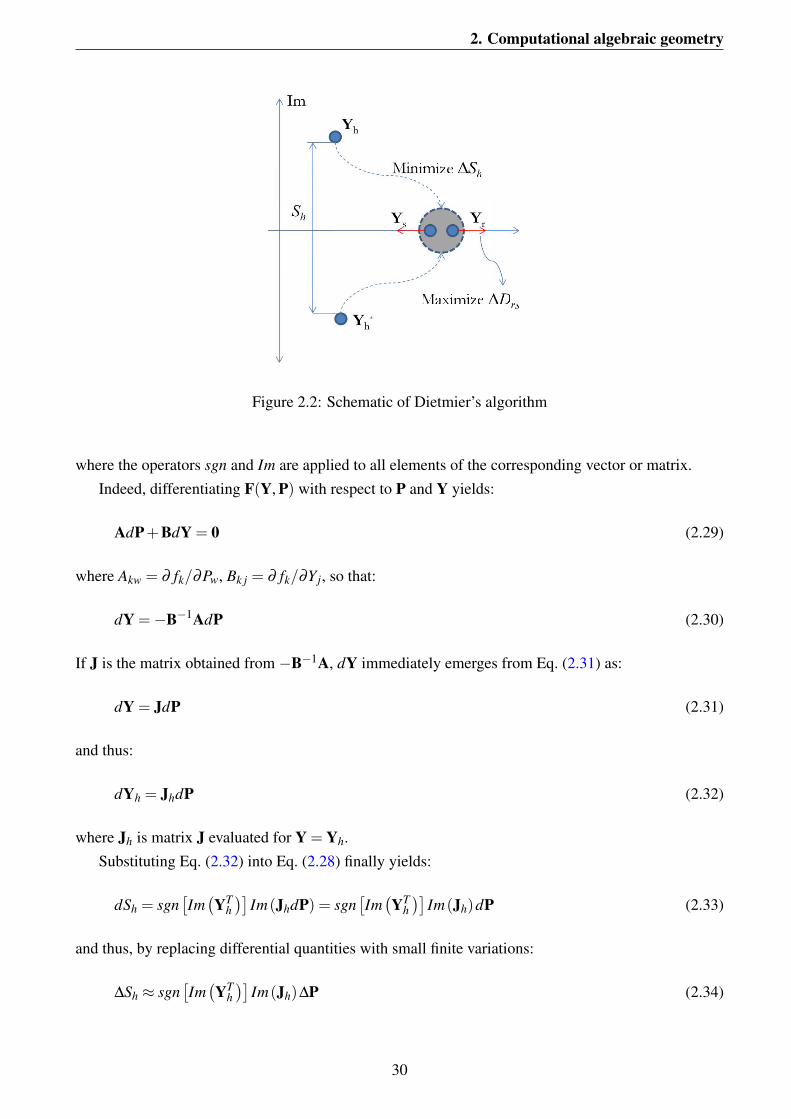
2. Computational algebraic geometry
Figure 2.2: Schematic of Dietmier’s algorithm
where the operators sgn and Im are applied to all elements of the corresponding vector or matrix.Indeed, differentiating F(Y, P) with respect to P and Y yields:
AdP+BdY = 0 (2.29)
where Akw = ∂ fk/∂Pw, Bk j = ∂ fk/∂Yj, so that:
dY =−B−1AdP (2.30)
If J is the matrix obtained from −B−1A, dY immediately emerges from Eq. (2.31) as:
dY = JdP (2.31)
and thus:
dYh = JhdP (2.32)
where Jh is matrix J evaluated for Y = Yh.Substituting Eq. (2.32) into Eq. (2.28) finally yields:
dSh = sgn[Im(YT
h)]
Im(JhdP) = sgn[Im(YT
h)]
Im(Jh)dP (2.33)
and thus, by replacing differential quantities with small finite variations:
∆Sh ≈ sgn[Im(YT
h)]
Im(Jh)∆P (2.34)
30
2. Computational algebraic geometry
By Eq. (2.34), the task of bringing two complex conjugate solutions closer together is reduced tosearching for a vector ∆P that minimises the objective function, ∆Sh. This is a linear optimisationproblem, which may be solved by any algorithm for linear programming, such as the simplex method(Luenberger and Ye [2008]).
Since the formulation given in Eq. (2.34) emerges from the linearisation of a complex nonlinearsystem of equations, the estimation that it provides is acceptable so long as ∆P is sufficiently small;that is:
−∆Pmax ≤ ∆P≤ ∆Pmax (2.35)
where, for the sake of simplicity, all components of ∆Pmax are taken to be equal to a given ∆Pmax.Furthermore, when the distance between any two real solutions associated with the current value
of P reaches a certain minimal value, Dmin, the algorithm must ensure that they do not become anycloser so as to prevent them eventually forming a complex conjugate pair. If Yr and Ys are any twosuch poses, differentiating Eq. (2.26) and further using Eq. (2.32) yields:
dDrs = 2(Yr−Ys)T (dYr−dYs) = 2(Yr−Ys)
T (Jr−Js)dP (2.36)
Accordingly, the condition that Yr and Ys must not become any closer when assigning the increment∆P may be expressed by the linear constraint:
(Yr−Ys)T (Jr−Js)∆P≥ 0 (2.37)
By considering Eqs. (2.34), (2.35) and (2.37), the linear optimisation problem may be stated as:
minimise : sgn[Im(YT
h
)]Im(Jh)∆P
subject to : −∆Pmax ≤ ∆P≤ ∆Pmax;(Yr−Ys)
T (Jr−Js)∆P≥ 0, ∀(Yr, Ys) : Drs < Dmin
(2.38)
If the problem in Eq. (2.38) provides a solution, the corresponding increment, ∆P, is added to P andthe set of geometric parameters is updated. The solutions of the modified F(Y, P) are then computed bythe help of an iterative Newton-Raphson routine, using Yh+Jh∆P, h = 1 . . .Nsol , as a starting estimate.At this point, the distance-reduction procedure formulated in Eq. (2.38) may be attempted again.
By the iterative application of the aforementioned minimisation procedure, Sh is progressively re-duced until the imaginary parts of all elements of Yh become smaller than a certain numerical error, ε .In this situation, Yh and Yh may be, from a numerical point of view, either complex conjugate or real.A Newton-Raphson algorithm is then used to search in a sphere of radius ε , centred at ℜ(Yh), for twodistinct real solutions, Yu and Yv, so that Yu and Yv may replace Yh and Yh. In order to prevent Yu andYv changing back to the complex field in the following steps of the algorithm, they are subsequentlyforced apart in the real domain by a certain distance (see Section 2.3.3). At this point, the algorithm isready to attempt the transformation of another pair of complex conjugate roots into real ones. The pair
31
2. Computational algebraic geometry
that is chosen is always that which has the shortest distance Sh.
2.3.3 Increasing the distance between a pair of real solutions
Let Yu and Yv be two real equilibrium poses. A variation, ∆P, of the parameter vector needs to becomputed such that the distance between them, Duv, is increased. If ∆P is sufficiently small, theincrement of Duv may be expressed as in Eq. (2.36), so that maximising ∆Duv may be reduced toa linear maximisation problem subject to the same constraints (Eqs. (2.35) and (2.37)) discussed inSection 2.3.2; that is,
maximize : (Yu−Yv)T (Ju−Jv)∆P
subject to : −∆Pmax ≤ ∆P≤ ∆Pmax;(Yr−Ys)
T (Jr−Js)∆P≥ 0, ∀(Yr, Ys) : Drs < Dmin
(2.39)
The procedure in Eq. (2.39) is repeated until either Duv reaches a convenient value, Dr (e.g. 2Dmin),or no ∆P is found that satisfies the imposed constraints.
32

Chapter 3
Geometric Static model of under-constrainedcable-driven parallel robot
It is well-known in robotics that under conditions of static equilibrium, an external wrench, w, appliedto an end-effector relates to actuation forces, τ , as follows:
JTτ +w = 0 (3.1)
where J is the jacobian matrix that transforms end-effector twists into actuator velocities. As such,for a platform in a given posture with given wrench, w, the applied force on the cables, τ , may beobtained as the solution of Eq. (3.1). In general, for f -DOF end-effector and n tendons, J is a matrix ofsize f ×n. Based on the dimensions of the jacobian matrix, J, a classification of cable-driven parallelrobots is defined. This was first proposed by Ming and Higuchi [1994] and discussed in further detailby Kurtz and Hayward [1991]; Roberts et al. [1998]. When the number of cables is more than thedegrees of freedom of the moving platform; that is:
n > f (3.2)
the forces in the cables are computed as:
τ =−JT+w+λh (3.3)
where JT+ is the pseudo-inverse of matrix JT , h is an arbitrary vector in the null space of JT and λ isa free parameter. One of the special characteristics of cables that makes the control of the end-effectorchallenging is that the cable cannot withstand compression. Therefore, in a cable-driven parallel robotwith n cables and the moving platform at rest in equilibrium, the following condition must be satisfied:
τi ≥ 0, i = 1, 2, . . .n (3.4)
33
3. Mathematical geometric static model of CDPRs
where τi is the applied force in each cable. Provided that all the components of h in Eq. (3.6) arepositive, λ may be set sufficiently large to ensure that all the applied forces in the cables are positiveregardless of w. Physically, the outcome of this is that the position and orientation of the robot areindependent of the imposed load, w, on the end-effector.
In the case of a robot with the number of cables, n, equal to the number of degrees of freedom, thatis:
n = f (3.5)
the forces in the cables are computed as:
τ =−J−1w (3.6)
When the robot falls into configurations with positive tension in all cables, the pose of the moving plat-form is independent of the imposed load and may be controlled by changing the cable lengths. Theseconfigurations in which it is impossible for the robot to be moved from its position and orientationwithout having to change the cable lengths are called fully constrained.
On the other hand, when the number of cables is less than the number of DOFs; that is:
n < f (3.7)
then, in general, Eq. (3.1) has no solution unless it satisfies the consistency condition. From a mathe-matical point of view, Eq. (3.1) has solutions only if the external wrench w falls into the column spaceof JT . Under this condition, from linear algebra, a solution of the forces in the cables, τ , may be com-puted for an imposed wrench w. But even if all the forces of the cables be computed as positive, stillsome freedoms of the platform can not be controlled because of the condition in Eq. (3.7). Physically,this means that the posture of the moving platform depends on the imposed load, in addition to thecable lengths, since when the load changes the pose has to adapt in order to satisfy the consistencycondition. In practice, due to the external wrench, the platform pasture may change even if the cablelengths are kept constant. Such a system in which the posture of the moving platform depends onapplied load is called under-constrained. Due to the increased complexity of displacement analysis forsuch a robot, where kinematics and statics must be dealt with simultaneously, an appropriate math-ematical model for the robot is necessary to solve the problem efficiently. In the following section,modelling of such a robot and derivation of the governing equations are discussed.
3.1 Mathematical geometric static model of CDPRs
As shown in Fig. 3.1, a general under-constrained n-n CDPR comprises a mobile platform connectedto a fixed base by n < 6 cables. The ith cable (i = 1, 2, ...n) is attached to the base at point Ai and tothe platform at point Bi. It is assumed that the platform is acted upon by a 0-pitch wrench, w = QLe,applied at point G, where Q is the constant magnitude of w and Le is the normalised Plucker vector
34
3. Mathematical geometric static model of CDPRs
of its line of action. Such a wrench may, for example, result from the weight of the platform actingthrough its centre of mass. To formulate the problem, other relevant definitions are as follows:
• Oxyz is a Cartesian coordinate frame fixed to the base with i, j and k being unit vectors along thecoordinate axes.
• O′x′y′z′ is a Cartesian coordinate frame fixed to the end-effector with i′, j′ and k′ being thecorresponding unit vectors along the coordinate axes.
• The platform posture is described by X = [x;Φ], where x = O′−O and Φ is the array groupingthe variables that parameterise the platform orientation with respect to Oxyz.
• ρi is the cable length.
• ai = Ai−O, ri = Bi−O′, si = Bi−Ai and ui = (Ai−Bi)/ρi =−si/ρi.
• bi is the projection of ri on O′x′y′z′.
• R(Φ) is the rotation matrix between the mobile and fixed frame.
• ri = R(Φ)bi.
• Li/ρi is the normalised Plucker vector of the ith cable in axis coordinates.
• pi is any vector from an arbitrarily-chosen reference point P (called for brevity moment pole) tothe cable line.
• Li =− [si;pi× si].
• τi is a scalar representing the cable tensile force.
• (τi/ρi)Li is the wrench exerted by the ith cable on the platform.
For the sake of brevity, the components of x in Oxyz are denoted as x, y and z. Vector componentsalong the coordinate axes are denoted by righthand subscripts reporting the axes names.
For practical reasons, the following is finally assumed:
1. ρi > 0 and, thus, si 6= 0, i = 1 . . .n (Assumption 1);
2. 0 < ||B j−Bi||< ||(A j−Ai)xy||, i 6= j (Assumption 2).
The latter assumption, according to which the segment BiB j is strictly smaller than the projection ofthe segment AiA j on the xy-plane, is not conceptually necessary, but it rules out some special configu-rations, which could be handled with no difficulty, but whose analysis would burden the presentation.In particular, the possibility that any two cables may be simultaneously parallel to k is discarded.
It will now be shown that, according to the problem under consideration, the governing equationscan be simplified by appropriately choosing the reference coordinates and the orientation of the axes.
35
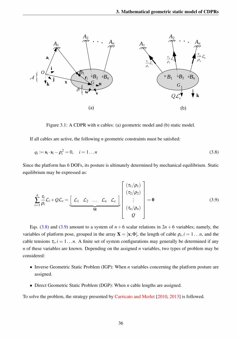
3. Mathematical geometric static model of CDPRs
A
B
A1
A2An
B1B2
GBn
A1
A2An
B1 B2 Bn
11
1
τρL
22
2
τρL
nn
n
τρL
O
xri
i
jk u
vw
ai
G
eLQ{
{k
(a) (b)
Figure 3.1: A CDPR with n cables: (a) geometric model and (b) static model.
If all cables are active, the following n geometric constraints must be satisfied:
qi := si · si−ρ2i = 0, i = 1 . . .n (3.8)
Since the platform has 6 DOFs, its posture is ultimately determined by mechanical equilibrium. Staticequilibrium may be expressed as:
n
∑i=1
τi
ρiLi +QLe =
[L1 L2 . . . Ln Le
]︸ ︷︷ ︸
M
(τ1/ρ1)
(τ2/ρ2)...
(τn/ρn)
Q
= 0 (3.9)
Eqs. (3.8) and (3.9) amount to a system of n+ 6 scalar relations in 2n+ 6 variables; namely, thevariables of platform pose, grouped in the array X = [x;Φ], the length of cable ρi, i = 1 . . .n, and thecable tensions τi, i = 1 . . .n. A finite set of system configurations may generally be determined if anyn of these variables are known. Depending on the assigned n variables, two types of problem may beconsidered:
• Inverse Geometric Static Problem (IGP): When n variables concerning the platform posture areassigned.
• Direct Geometric Static Problem (DGP): When n cable lengths are assigned.
To solve the problem, the strategy presented by Carricato and Merlet [2010, 2013] is followed.
36
3. Mathematical geometric static model of CDPRs
Both problems may be simplified by eliminating cable tensions from Eq. (3.9). A convenientelimination strategy emerges by observing that Eq. (3.9) holds only if:
rank(M)≤ n (3.10)
namely if L1,L2, . . .Ln and Le are linearly dependent. This is a purely geometric condition, since Mis a 6× (n+ 1) matrix depending only on the platform posture. Furthermore, such relations do not
comprise cable lengths and lead to a partial decoupling of the system equations, with cable lengthsappearing only in Eq. (3.8). The IGP takes particular advantage of the aforementioned decoupling,as the platform configuration may be directly computed by relations emerging from Eq. (3.10). Bysetting all (n+1)× (n+1) minors of M equal to zero and by conveniently changing the moment pole,a large set of linearly independent relations exclusively comprising the platform pose variables may bederived; that is:
pk (X) = 0, k = 1 . . .Np (3.11)
where Np is an integer, usually much greater than the number of variables, NX , contained in X. Indeed,for Eq. (3.10) to hold, all minors of M must vanish and this ordinarily results in more equations thanthe number of variables, NX . The solution of the IGP problem coincides with the variety, V , of the idealgenerated by such equations. When n configuration variables are known (typically, either x or Φ), anyset of n equations from Eq. (3.11) may be chosen and a corresponding (generally zero-dimensional)variety, V , is obtained. Once X is known, cable lengths may be directly calculated by Eq. (3.8).It is worth emphasising that the IGP only provides potential robot configurations, since, when thecable lengths emerging from Eq. (3.8) are fed into the actuators of the actual robot, the end-effectormay evolve, a priori, in any one of the feasible solutions emerging from the corresponding DGP andnothing guarantees that the desired configuration is actually attained. This will be discussed in moredetail later on. The DGP poses remarkably more complex mathematical problems, as in this case, theplatform configuration is entirely unknown and it must be determined by simultaneously satisfyingboth the relations emerging from Eq. (3.11) and those emerging from Eq. (3.8).
The cost of eliminating some of the unknowns is that the relations in Eq. (3.11) are significantlymore involved than those in Eq. (3.9). In particular, when they are of polynomial form, as is normallythe case, they have a higher degree, more numerous terms and more complicated coefficients. Formu-lating equilibrium constraints via Eq. (3.11) is particularly favourable if, in order to solve the DGP,variable-elimination strategies are pursued that take advantage of the abundance of linearly indepen-dent relations that this approach provides, such as methods based on Groebner bases or Sylvester’sdialytic elimination (Carricato [2013a,b]; Carricato and Merlet [2011a,b]). These methods, however,rely on exact-arithmetic calculations and are particularly expensive in terms of computational burden.When working with floating-point computation (such as homotopy continuation or interval analysis),the relations in Eq. (3.11) have two drawbacks. Firstly, they are very sensitive to the accuracy withwhich the coefficients are calculated, such that solutions are appreciably affected by numerical errors.
37
3. Mathematical geometric static model of CDPRs
Furthermore, in order to compute a finite set of solutions, a subset of NX −n relations must be selectedwithin Eq. (3.11), so as to form, together with Eq. (3.8), a square system of NX equations in NX un-knowns. In this way, only a few minors of M are used and spurious roots are likely to be introduced;that is, solutions for which some of the unused minors do not vanish. Accordingly, all roots must bechecked against the original set of equations, thus further increasing the computational burden. Dueto these limits, the formulation of static equilibrium via Eq. (3.9) will be preferred for the successfulimplementation of numerical continuation methods.
Since using different parameterisations to describe the platform configuration causes Eqs. (3.8),(3.9) and (3.11) to yield polynomial relations with varied complexity and degree, alternative parame-terisations will now be discussed.
3.2 Rodrigues’ parameterisation
According to Rodrigues’ parametrisation, the platform posture, X, may be described by 6 variables;namely, the vector x identifying the position of a point on the platform (e.g. O′) and the array Φ
grouping the three Rodrigues parameters defining the platform orientation with respect to the fixedframe. Rodrigues parameters are derived using the theorem of Cayley (Bottema and Roth [1990]).This theorem states that it is possible to represent an orthogonal matrix, R, using a skew symmetricmatrix, S:
R = (I−S)−1(I+S) (3.12)
where I is the 3×3 unit matrix and
S =
0 −e3 e2
e3 0 −e1
−e2 e1 0
(3.13)
If the eigenvalues of R do not have values of −1 (meaning that R does not describe a rotation ofangle π), one may compute the matrix S via S = (R− I)(R+ I)−1. From the entries ei of S, one candirectly compute the direction of the rotation axis Φ = (e1, e2, e3) and the rotation angle tan(φ
2 ) =√e2
1 + e22 + e2
3. The parameters ei, i = 1, . . . , 3 are called Rodrigues parameters. The case in which Rdescribes a rotation of angle π must be handled in a different way, as shown by Angeles [2002].
Accordingly, XT = [xT ;ΦT ]. Substitution of these variables into Eqs. (3.8) and (3.9) provides n+6
scalar relations in 2n+ 6 variables; that is, x, Φ and τ . This parameterisation is especially suitablewhen the elimination strategy is implemented, as it only introduces the minimum number of variables.Accordingly, the number of elimination steps and the required time are reduced.
It is worth mentioning a drawback of this parameterization when the Dietmaier algorithm, discussedin Section 2.3, is applied. This parameterisation involves variables with mixed units (the componentsof x are lengths, whereas those of Φ are dimensionless), making it difficult to conceive a physically-
38
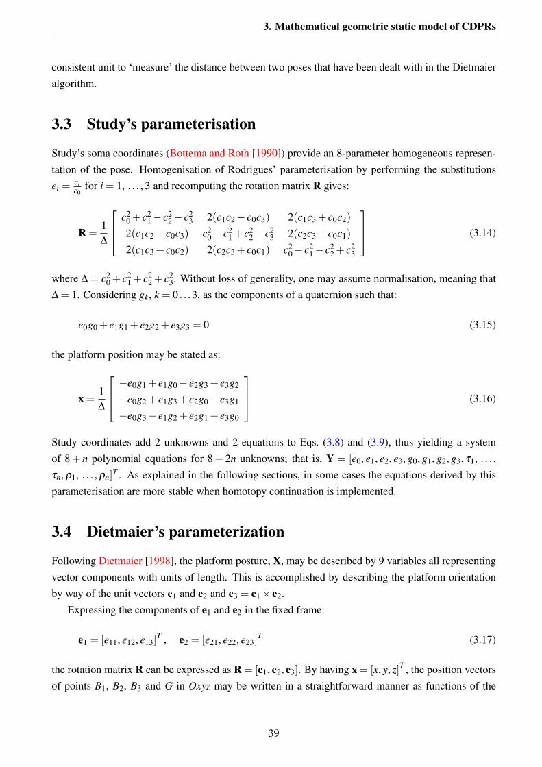
3. Mathematical geometric static model of CDPRs
consistent unit to ‘measure’ the distance between two poses that have been dealt with in the Dietmaieralgorithm.
3.3 Study’s parameterisation
Study’s soma coordinates (Bottema and Roth [1990]) provide an 8-parameter homogeneous represen-tation of the pose. Homogenisation of Rodrigues’ parameterisation by performing the substitutionsei =
cic0
for i = 1, . . . , 3 and recomputing the rotation matrix R gives:
R =1∆
c20 + c2
1− c22− c2
3 2(c1c2− c0c3) 2(c1c3 + c0c2)
2(c1c2 + c0c3) c20− c2
1 + c22− c2
3 2(c2c3− c0c1)
2(c1c3 + c0c2) 2(c2c3 + c0c1) c20− c2
1− c22 + c2
3
(3.14)
where ∆ = c20 + c2
1 + c22 + c2
3. Without loss of generality, one may assume normalisation, meaning that∆ = 1. Considering gk, k = 0 . . .3, as the components of a quaternion such that:
e0g0 + e1g1 + e2g2 + e3g3 = 0 (3.15)
the platform position may be stated as:
x =1∆
−e0g1 + e1g0− e2g3 + e3g2
−e0g2 + e1g3 + e2g0− e3g1
−e0g3− e1g2 + e2g1 + e3g0
(3.16)
Study coordinates add 2 unknowns and 2 equations to Eqs. (3.8) and (3.9), thus yielding a systemof 8+ n polynomial equations for 8+ 2n unknowns; that is, Y = [e0, e1, e2, e3, g0, g1, g2, g3, τ1, . . . ,τn, ρ1, . . . , ρn]
T . As explained in the following sections, in some cases the equations derived by thisparameterisation are more stable when homotopy continuation is implemented.
3.4 Dietmaier’s parameterization
Following Dietmaier [1998], the platform posture, X, may be described by 9 variables all representingvector components with units of length. This is accomplished by describing the platform orientationby way of the unit vectors e1 and e2 and e3 = e1× e2.
Expressing the components of e1 and e2 in the fixed frame:
e1 = [e11, e12, e13]T , e2 = [e21, e22, e23]
T (3.17)
the rotation matrix R can be expressed as R = [e1, e2, e3]. By having x = [x, y, z]T , the position vectorsof points B1, B2, B3 and G in Oxyz may be written in a straightforward manner as functions of the
39
3. Mathematical geometric static model of CDPRs
array:
X = [x, y, z, e11, e12, e13, e21, e22, e23]T (3.18)
whose components satisfy the conditions:
e211 + e2
12 + e213 = 1,
e221 + e2
22 + e223 = 1,
e11e21 + e12e22 + e13e23 = 0
(3.19)
When the geometric parameters of a robot are known, Eqs. (3.8), (3.9) and (3.19) form a system ofn+9 scalar relations with 2n+9 variables, namely x = [x, y, z], ρi, τi, i = 1 . . .n, and
Y = [e11, e12, e13, e21, e22, e23]T (3.20)
Dietmaier’s parameterisation introduces a higher number of variables, making it unsuitable for theelimination procedures. On the other hand, when dealing with continuation methods, this type ofparameterisation is preferred over the Rodrigues variation due to the fact that it yields simpler lower-order polynomial equations, which prove to be stabler. Furthermore, as explained in Section 2.3,when Dietmaier’s algorithm is implemented, parameterisation of the platform pose is homogeneous interms of units of measurement, which is an advantage for conceiving a physically consistent way of‘measuring’ the distance between two poses.
40
Chapter 4
Problem-solving algorithm for the geometricstatic problem of under-constrained CDPRs
This chapter presents analysis results for the geometric static problem of under-constrained cabledriven parallel robots. By implementing the tools discussed in the previous chapter, inverse and di-rect geometric static problems for robots with 2, 3 . . . , 5 cables are solved. Within the problem-solvingalgorithm, the following issues, which are classic challenges in robot analysis, are specifically dealtwith:
1. determination of the number of solutions in the (zero-dimensional) algebraic variety defined bythe polynomial equations of the problem;
2. reduction of the problem to a single equation with one unknown;
3. numerical computation of the solution set;
4. identification of a specific geometry providing the maximum number of distinct real-valued so-lutions.
By implementing appropriate elimination strategies for the respective IGPs and DGPs, the first twoabove mentioned issues have been resolved for robots with n≤ 5 cables. The strategies are explainedin detail in Section 4.1. It will be shown that when a DGP is dealt with, the elimination strategiesyield univariate equations of very high order. Due to the complexity of these equations, numericalprocedures are introduced in Section 4.2 to compute the solutions of the DGP efficiently. The last issuementioned above is especially challenging when dealing with DGPs. Due to the very high order of theunivariate polynomials and the complexity of the corresponding equations, it is difficult to identify arobot geometry with the maximum number of real solutions. Accordingly, as discussed in Section 4.3,the Dietmaier algorithm is applied to overcome this problem.
41
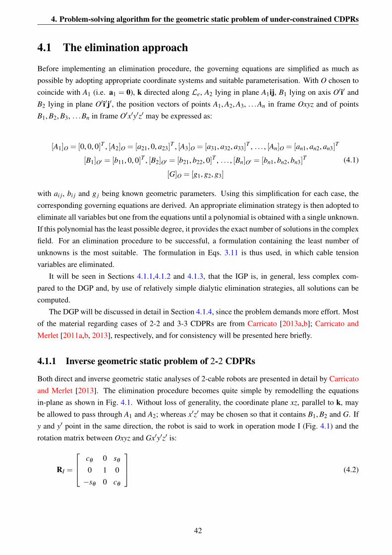
4. Problem-solving algorithm for the geometric static problem of under-constrained CDPRs
4.1 The elimination approach
Before implementing an elimination procedure, the governing equations are simplified as much aspossible by adopting appropriate coordinate systems and suitable parameterisation. With O chosen tocoincide with A1 (i.e. a1 = 0), k directed along Le, A2 lying in plane A1ij, B1 lying on axis O′i′ andB2 lying in plane O′i′j′, the position vectors of points A1, A2, A3, . . .An in frame Oxyz and of pointsB1, B2, B3, . . .Bn in frame O′x′y′z′ may be expressed as:
[A1]O = [0, 0, 0]T , [A2]O = [a21, 0, a23]T , [A3]O = [a31, a32, a33]
T , . . . , [An]O = [an1, an2, an3]T
[B1]O′ = [b11, 0, 0]T , [B2]O′ = [b21, b22, 0]T , . . . , [Bn]O′ = [bn1, bn2, bn3]T
[G]O = [g1, g2, g3]
(4.1)
with ai j, bi j and g j being known geometric parameters. Using this simplification for each case, thecorresponding governing equations are derived. An appropriate elimination strategy is then adopted toeliminate all variables but one from the equations until a polynomial is obtained with a single unknown.If this polynomial has the least possible degree, it provides the exact number of solutions in the complexfield. For an elimination procedure to be successful, a formulation containing the least number ofunknowns is the most suitable. The formulation in Eqs. 3.11 is thus used, in which cable tensionvariables are eliminated.
It will be seen in Sections 4.1.1,4.1.2 and 4.1.3, that the IGP is, in general, less complex com-pared to the DGP and, by use of relatively simple dialytic elimination strategies, all solutions can becomputed.
The DGP will be discussed in detail in Section 4.1.4, since the problem demands more effort. Mostof the material regarding cases of 2-2 and 3-3 CDPRs are from Carricato [2013a,b]; Carricato andMerlet [2011a,b, 2013], respectively, and for consistency will be presented here briefly.
4.1.1 Inverse geometric static problem of 2-2 CDPRs
Both direct and inverse geometric static analyses of 2-cable robots are presented in detail by Carricatoand Merlet [2013]. The elimination procedure becomes quite simple by remodelling the equationsin-plane as shown in Fig. 4.1. Without loss of generality, the coordinate plane xz, parallel to k, maybe allowed to pass through A1 and A2; whereas x′z′ may be chosen so that it contains B1, B2 and G. Ify and y′ point in the same direction, the robot is said to work in operation mode I (Fig. 4.1) and therotation matrix between Oxyz and Gx′y′z′ is:
RI =
cθ 0 sθ
0 1 0−sθ 0 cθ
(4.2)
42

4. Problem-solving algorithm for the geometric static problem of under-constrained CDPRs
A1≡O
k
z
x
A2
B1B2
a2
r1 r2
eQ
x'
z'
θ
r12
A1≡O
k
z
x
A2
B1B2
a2
r1 r2
eQ
x'
z'
r12
G
Gθ
(a) (b)
Figure 4.1: Geometric model of a cable-driven parallel robot with 2 cables: (a) operation mode I; (b)operation mode II (Carricato and Merlet [2013])
Whereas if y and y′ point in opposite directions, the robot is said to work in operation mode II (Fig. 4.1)and the rotation matrix is:
RI =
cθ 0 sθ
0 −1 0sθ 0 −cθ
(4.3)
where θ is the angle formed by x′ and x with a positive rotation about y′ and sθ and cθ stand for sin(θ)
and cos(θ), respectively. If b′i is the coordinate vector of Bi in the Gx′y′z′ frame, then ri = RI(θ)b′i orri = RII(θ)b′i. By noting that in equilibrium conditions the two planes xz and x′z′ necessarily coincideand by considering O = A1 as the reduction pole of the moments, the matrix M in Eq. (3.9) may bereduced to:
M′ =
[−(x+ r1) a2− (x+ r2) k
0 −a2× (x+ r2) x×k
]=
x+ r1x r21x−a2x 0z+ r1z r21z−a2z 1
0 a2× (x+ r2) · j −x
(4.4)
Accordingly, Eq. (3.10) holds if and only if detM′ = 0; namely:
p1 := (r21xx+a2xr1x)z−r21zx2+(r1zr2x−r1xr2z+a2xr21z−a2zr2x)x+r1x(a2xr2z−a2zr2x) = 0 (4.5)
The two constraint equations emerging from Eq. (3.8) may be linearly combined in the form:
p2 := x2 + z2 +2(r1xx+ r1zz)+‖r1‖2−ρ12 = 0
p3 := 2(a2x− r21x)x+2(a2z− r21z)z+‖r1‖2−‖a2− r2‖2 +ρ22−ρ1
2 = 0(4.6)
43
4. Problem-solving algorithm for the geometric static problem of under-constrained CDPRs
comprising the variables x, z, θ , ρ1 and ρ2.The inverse problem of a 2-2 CDPR may be solved by considering only Eq. (4.5). Following Car-
ricato and Merlet [2013], 4 different cases may be distinguished depending on which pose parametersare assigned:
1. The orientation θ and variable x are assigned:
In this case, Eq. (4.5) provides a single solution in z, except for the case in which r21xx=−a2xr1x.If the latter condition occurs, the problem may only be solved if the entire polynomial vanishes,in which case the solution set is one-dimensional and coincides with a line parallel to k. Thisoccurs if either one of the following conditions holds:
• rix = 0 and x = aix, with i = 1 or 2;
• a2× r21 · j = 0, r21x 6= 0 and x =−a2xr1x/r21x.
In the former case, Ai, Bi and G lie on a line parallel to k and the robot operates as a 1-DOF cranewith the ith cable holding the entire load. In the latter case, the line segments A1A2 and B1B2
are parallel and the platform may follow a quasi-static linear path parallel to k, with orientationbeing constant and the load being sustained by both cables.
2. The orientation θ and variable z are assigned:
In this case, Eq. (4.5) provides, in general, two solutions for x. If all coefficients of p1 vanish,the solution set is one-dimensional and coincides with a line perpendicular to k. p1 is identicallynought if r1z = r2z, z+ r1z = a jz and rix = 0, with i 6= j; namely, if points B1, B2 and A j lie on aline perpendicular to k.
3. The orientation θ and an approximate location of G are assigned:
If the orientation and an approximate desired location, (xd , zd), of G are assigned, x and z mustbe found such that Eq. (4.5) is satisfied and the error, ε = (x− xd)
2 +(z− zd)2, is minimised.
Since both ε and p1 are continuously differentiable in x and z, the global minimum of ε is astationary point of the function Lε = (x− xd)
2 +(z− zd)2 +λ p1(x, z). Setting the derivatives of
Lε with respect to x and z to zero provides a linear system in x and z, by which both variablesmay be determined as functions of λ . Upon substituting x = x(λ ) and z = z(λ ) into p1, a fourth-degree polynomial in λ is obtained. Its real roots are the stationary points of Lε , among which theglobal minimum may be determined by direct evaluation of ε . Clearly, this optimal configurationis feasible only if the conditions concerning the sign of cable tensions and stability are satisfied.
4. The position (x, y) is assigned:
Letting ri = RI(θ)bi or ri = RII(θ)bi, with i = 1 and 2, p1 becomes a quadratic polynomial insθ and cθ . For each operational mode, the resultant of p1 and the trigonometric identity withrespect to cθ yields a fourth-degree equation in sθ . For each root in sθ , Eq. (4.5) provides asingle value of cθ and thus of θ . The problem admits altogether 8 solutions, all of which may bereal.
44

4. Problem-solving algorithm for the geometric static problem of under-constrained CDPRs
4.1.2 Inverse geometric static problem of 3-3 CDPRs
For the case of robot with 3 cables, Eqs. (3.8) and (3.9) amount to 9 scalar relations in 12 variables.Two cases of the IGP are studied, depending on which set of 3 platform posture variables are assigned:
1. IGP with assigned orientation in which Φ and, correspondingly, all vectors ri, i = 1 . . .3, areknown.
2. IGP with assigned position in which x is given and r1, r2 and r3 are unknown
4.1.2.1 Inverse geometric static problem of 3-3 CDPR with assigned orientation
When Φ is assigned, all vectors ri, i = 1 . . .3, are known. If O is chosen as the reduction pole ofmoments, Li andLe may be expressed, in axis coordinates, as− [si; ai× si] and [k; x×k], respectively.Accordingly, M in Eq. (3.9) becomes:
M(O) =
[−s1 −s2 −s3 k
0 −a2× s2 −a3× s3 x×k
](4.7)
or, equivalently, by setting si = x+ ri−ai and by performing elementary column transformations:
M′(O) =
[x+ r1 r21−a2 r31−a3 k
0 a2× (x+ r2) a3× (x+ r3) x×k
](4.8)
where ri j = ri− r j, i 6= j.It is important to observe that letting Bi ≡ Ai, with i = 1 . . .3, causes the ith column of M to vanish
(since si = ai× si = 0) and, thus, it causes all 4×4 minors of M (and of M′) to be zero. It follows thata configuration for which Bi ≡ Ai is a formal solution of the problem, as long as it is compatible withthe assigned constraints. We call it a trivial solution, and we need to discard it, since ρ is required tobe strictly positive:
xi := [xi, yi, zi]T = ai− ri, i = 1 . . .3. (4.9)
This observation is particularly important for the IGP with assigned orientation. In this case, infact, it is always possible to displace the platform (with a given orientation) so as to superimpose Bi
onto Ai. Consequently, all trivial solutions appear as solutions of the problem and need to be discarded.According to Eq. (3.11), the rank of the block matrix M′123(O) must be equal to either 2 or 3.
Discarding the trivial solutions and letting
∆ := detM′123, 234(O) = (r21−a2)x (r31−a3)y− (r21−a2)y (r31−a3)x (4.10)
two cases may be distinguished depending on ∆ being zero or not. It should be noted that ∆ dependsonly on the input parameters when Φ is assigned. For physical interpretation of each case, the readeris referred to Carricato [2013a]; Carricato and Merlet [2011a].
45
4. Problem-solving algorithm for the geometric static problem of under-constrained CDPRs
1. ∆ 6= 0 :
Equations
p1 := detM′1236(O) = A20x2− (B011 +C101)xy
+A02y2 +A10x+A01y+A00 = 0(4.11a)
p2 := detM′1235(O) = B110xy−A20xz+B020y2
+B011yz+B100x+B010y+B001z+B000 = 0(4.11b)
p3 := detM′1234(O) = B110x2 +B020xy−C101xz
+A02yz−C100x−C010y−C001z−C000 = 0(4.11c)
comprise the lowest-degree polynomials among all minors of M′(O), with coefficients Ai j, Bi jk
and Ci jk being functions of the geometric and orientation parameters only. Since rankM′123(O) =
3, satisfying Eqs. (4.11a)-(4.11c) assures that rankM′(O) = rankM′123(O) and thus the variety,V , generated by Eq. (3.11) is equivalent to the variety, V123, generated by the above three equa-tions.
p1 is quadratic in x and y and does not contain the variable z. p2 and p3 are quadratic in x, y andz but do not contain the monomial z2. Eliminating z from p2 and p3 gives a cubic polynomial,p23, in x and y; whereas eliminating y from p1 and p23 yields a 4th degree equation in x; namely:
p123 :=4
∑h=0
Ehxh = 0 (4.12)
It emerges from Eqs. (4.11a)-(4.11c) that the coefficients of the leading monomials y2 and y3 inp1 and p23 are, respectively, A02 and A02B020 with, in particular, A02 = a3xr21x−a2xr31x. SinceA02 appears in both coefficients, it factors all terms of the resultant of p1 and p23 with respect toy. p123 is the polynomial obtained by eliminating A02 from such a resultant. This simplificationis obvious when A02 6= 0, but it is still valid when A02 = 0, with a caveat. In fact, if the resultantof p1 and p23 is calculated after setting A02 = 0, a 4th-degree polynomial in x is again obtainedand it proves to be equal to p123 times the constant:
Γ0 := B020(C001 +A01)−C010B011 (4.13)
Hence, as long as Γ0 6= 0, p123 is still a legitimate elimination ideal for p1 and p23. The caseΓ0 = 0 is discussed by Carricato [2013a]. Since three roots of p123 necessarily correspond to
46
4. Problem-solving algorithm for the geometric static problem of under-constrained CDPRs
trivial solutions, the fourth root, x4, must be real and may be computed by Vieta’s formula:
x4 =E0
x1x2x3E4=
E0
E4(4.14)
where the latter expression takes advantage of the fact that it is possible to factorise E0 and E4
as x1x2x3∆2E0 and ∆2E4, respectively. Once x4 is known, y4 may be calculated, for instanceas the greatest common divisor of p1 and p23, and z4 may be obtained by either Eq. (4.11b) orEq. (4.11c). As long as E4 6= 0, the problem thus admits a single real solution: x4 = (x4, y4, z4).Special combinations of the geometric parameters and input orientations for which Eqs. (4.11a)-(4.11c) admit infinite solutions are presented by Carricato [2013a]. In these cases, G may followquasi-static paths along assigned curves in space, with the platform orientation remaining con-stant.
2. ∆ = 0 :
By expanding the coefficients of p123, it is possible to verify that all of them comprise the factor∆2. Consequently, when ∆ = 0, p123 degenerates and the procedure described in the previoussection is not adequate to solve the problem.
Since it is assumed that (r21−a2)xy and (r31−a3)xy do not vanish, when ∆= 0 these two vectorsmust be parallel (Eq. (4.10)):
(r31−a3)xy = α (r21−a2)xy (4.15)
where α ∈ R−{0}.
By enforcing both Eq. (4.15) and ∆ = 0, the polynomial relations in Eq. (4.11) may be factoredas:
p1 := f10g = 0 (4.16a)
p2 := f20g = 0 (4.16b)
p3 := f30g = 0 (4.16c)
where f10 and g are linear polynomials in x and y, and f20 and f30 are linear polynomials in x, y
and z. In particular:
g := detM′123, 124(O) = (y1− y2)x− (x1− x2)y+ x1y2− y1x2 (4.17)
where the coefficients multiplying x and y cannot vanish simultaneously, since this would infer(x1− x2)xy = (r21−a2)xy = 0.
Equation (4.16) holds if either f10 = f20 = f30 = 0 or g = 0. Since the former requirementamounts to a linear non-homogeneous system in x, y and z whose coefficient matrix is singular(and, hence, admits in general no solution), only the latter condition applies. Together with the
47

4. Problem-solving algorithm for the geometric static problem of under-constrained CDPRs
requisite ∆ = 0, this brings about that rankM′123(O) = 2, with the first row of M′(O) linearlydependent on the second and third rows. The problem may thus be solved by considering thesystem comprising the relation:
p4 := g = 0 (4.18)
and any two of the equations:
p5 := detM′2345(O) = 0 (4.19a)
p6 := detM′2346(O) = 0 (4.19b)
p7 := detM′2356(O) = 0 (4.19c)
where p5, p6 and p7 are cubic polynomials in x, y and z, with p6 and p7 being linear in z and p5
being quadratic in z.
If, for instance, p6 and p7 are considered, eliminating z gives a 4th degree polynomial, p67, inx and y. Further eliminating y from p4 and p67 yields a quartic equation in x, p467 = 0, whichadmits a single non-trivial solution. This solution formally coincides with the quotient E0/E4
at the right-hand side of Eq. (4.14), once E0 and E4 are expressed as functions of the geometricand orientation parameters. If M′236(O) has full rank, then rankM′(O) = rankM′236(O) = 3 andV =V467. In this case, ∆ = 0 and the axes of L1, L2, L3 and Le form a regulus on a hyperbolicparaboloid.
It may happen that, in special cases, p467 degenerates and the procedure described above is notadequate to solve the problem. Typically, this may occur when rankM′236 = 2. A different choiceof minors normally allows one to conclude the analysis.
4.1.2.2 Inverse geometric static problem of 3-3 CDPR with assigned position
In the case where x is assigned and r1, r2 and r3 are unknown, the relations in Eq. (4.11) assume aparticularly favourable structure if the platform orientation is described by means of Rodrigues param-eters.
Indeed, by letting ri = Rbi, i = 1 . . .3, and by clearing the nonzero denominator, 1+ e21 + e2
2 + e23,
p1, p2 and p3 become quartic polynomials in the Rodrigues parameters:
ph := ∑k=0...4
m=0...4−kn=0...4−k−m
Dh, kmnek1em
2 en3 = 0, h = 1 . . .3 (4.20)
The quartic polynomials in e1, e2 and e3 that emerge from the minors detM′1245(O), detM′1246(O) anddetM′1256(O) depend linearly on p1, p2 and p3 and may be discarded. A further quartic emerges bysetting detM′j456(O) = 0 for j = 1 . . .3, so that:
(x+ r1)[detM′456, 234(O)
]= 0 (4.21)
48
4. Problem-solving algorithm for the geometric static problem of under-constrained CDPRs
The variety defined by Eq. (4.21) comprises, other than the trivial solution x1 = a1− r1 =−r1, the setof configurations for which
p8 := detM′456, 234(O) = 0 (4.22)
Equation (4.22) is indeed of degree 4 in e1, e2 and e3 (as well as of degree 2 in x, y, z). All minorsof M′(O) not considered so far; namely, detM′1345(O), detM′1346(O), detM′1356(O), detM′2345(O),detM′2346(O) and detM′2356(O), instead yield sextic equations in the Rodrigues parameters. In orderto solve such a system of polynomials, Sylvester’s dialytic method is implemented as an appropriateelimination strategy.
An effective implementation of the strategy consists of deriving a larger set of linearly independentquartics. Let M be written by choosing a generic P as the reduction pole of moments; namely:
M(P) =
[· · · −si · · · k· · · −(Bi−P)× si · · · (G−P)×k
](4.23)
When P ≡ Bi and P ≡ Ai, i = 1 . . .3, the moment vector in the ith column vanishes, so that settingdetM j456(Bi) = 0 and detM j456(Ai) = 0 for j = 1 . . .3 yields, respectively:
si [detM456, km4(Bi)] = 0 (4.24)
and
si [detM456, km4(Ai)] = 0 (4.25)
with k, m ∈ {1, 2, 3}−{i}. In this way, the following equations may be obtained:
p9 := detM456, 234(B1) = 0 (4.26a)
p10 := detM456, 134(B2) = 0 (4.26b)
p11 := detM456, 134(A2) = 0 (4.26c)
p12 := detM456, 124(B3) = 0 (4.26d)
p13 := detM456, 124(A3) = 0 (4.26e)
Analogously, by defining a convenient additional point, G0, such that G−G0 = k, and by setting P≡G
and P≡ G0, one may also obtain:
p14 := detM456, 123(G) = 0 (4.27a)
p15 := detM456, 123(G0) = 0 (4.27b)
All polynomials p j, j = 9 . . .15, have degree 4 in the Rodrigues parameters (and degree 2 in thecomponents of x).
49
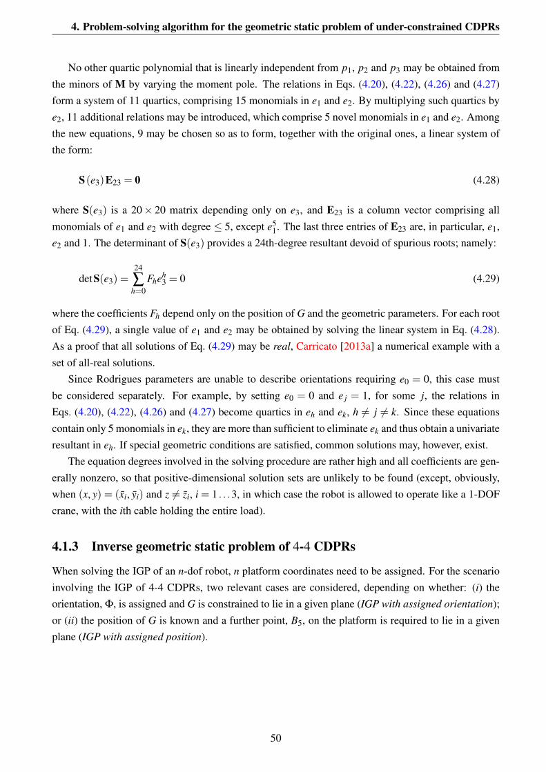
4. Problem-solving algorithm for the geometric static problem of under-constrained CDPRs
No other quartic polynomial that is linearly independent from p1, p2 and p3 may be obtained fromthe minors of M by varying the moment pole. The relations in Eqs. (4.20), (4.22), (4.26) and (4.27)form a system of 11 quartics, comprising 15 monomials in e1 and e2. By multiplying such quartics bye2, 11 additional relations may be introduced, which comprise 5 novel monomials in e1 and e2. Amongthe new equations, 9 may be chosen so as to form, together with the original ones, a linear system ofthe form:
S(e3)E23 = 0 (4.28)
where S(e3) is a 20× 20 matrix depending only on e3, and E23 is a column vector comprising allmonomials of e1 and e2 with degree ≤ 5, except e5
1. The last three entries of E23 are, in particular, e1,e2 and 1. The determinant of S(e3) provides a 24th-degree resultant devoid of spurious roots; namely:
detS(e3) =24
∑h=0
Fheh3 = 0 (4.29)
where the coefficients Fh depend only on the position of G and the geometric parameters. For each rootof Eq. (4.29), a single value of e1 and e2 may be obtained by solving the linear system in Eq. (4.28).As a proof that all solutions of Eq. (4.29) may be real, Carricato [2013a] a numerical example with aset of all-real solutions.
Since Rodrigues parameters are unable to describe orientations requiring e0 = 0, this case mustbe considered separately. For example, by setting e0 = 0 and e j = 1, for some j, the relations inEqs. (4.20), (4.22), (4.26) and (4.27) become quartics in eh and ek, h 6= j 6= k. Since these equationscontain only 5 monomials in ek, they are more than sufficient to eliminate ek and thus obtain a univariateresultant in eh. If special geometric conditions are satisfied, common solutions may, however, exist.
The equation degrees involved in the solving procedure are rather high and all coefficients are gen-erally nonzero, so that positive-dimensional solution sets are unlikely to be found (except, obviously,when (x, y) = (xi, yi) and z 6= zi, i = 1 . . .3, in which case the robot is allowed to operate like a 1-DOFcrane, with the ith cable holding the entire load).
4.1.3 Inverse geometric static problem of 4-4 CDPRs
When solving the IGP of an n-dof robot, n platform coordinates need to be assigned. For the scenarioinvolving the IGP of 4-4 CDPRs, two relevant cases are considered, depending on whether: (i) theorientation, Φ, is assigned and G is constrained to lie in a given plane (IGP with assigned orientation);or (ii) the position of G is known and a further point, B5, on the platform is required to lie in a givenplane (IGP with assigned position).
50
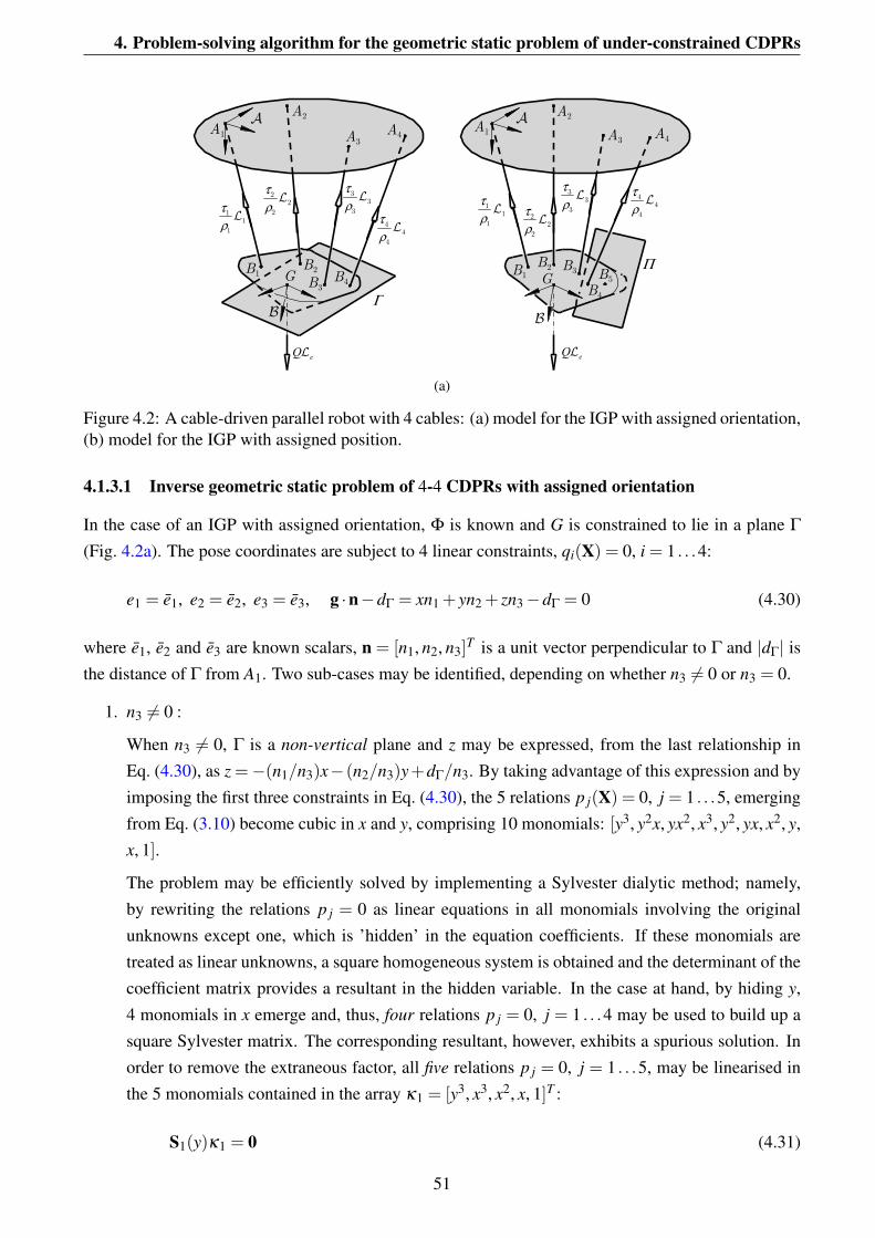
4. Problem-solving algorithm for the geometric static problem of under-constrained CDPRs
A1
A2
A3 A4
A
τρ
L11
1
τρ
L22
2
τρ
L33
3τρ
L44
4
B1B2
B3 B4 G
B
eQL
Γ
A1
A2
A3 A4
A
τρ
L11
1τρ
L22
2
τρ
L33
3
τρ
L4 4
4
B1B2 B3
B4G
B
eQL
Π B5
A1
A2
A3 A4
A
τρ
L1 1
1
τρ
L2 2
2
τρ
L3 3
3τρ
L4 4
4
B1 B2B3
B4 G
B
eQL
Γ
(a)
Figure 4.2: A cable-driven parallel robot with 4 cables: (a) model for the IGP with assigned orientation,(b) model for the IGP with assigned position.
4.1.3.1 Inverse geometric static problem of 4-4 CDPRs with assigned orientation
In the case of an IGP with assigned orientation, Φ is known and G is constrained to lie in a plane Γ
(Fig. 4.2a). The pose coordinates are subject to 4 linear constraints, qi(X) = 0, i = 1 . . .4:
e1 = e1, e2 = e2, e3 = e3, g ·n−dΓ = xn1 + yn2 + zn3−dΓ = 0 (4.30)
where e1, e2 and e3 are known scalars, n = [n1, n2, n3]T is a unit vector perpendicular to Γ and |dΓ| is
the distance of Γ from A1. Two sub-cases may be identified, depending on whether n3 6= 0 or n3 = 0.
1. n3 6= 0 :
When n3 6= 0, Γ is a non-vertical plane and z may be expressed, from the last relationship inEq. (4.30), as z =−(n1/n3)x− (n2/n3)y+dΓ/n3. By taking advantage of this expression and byimposing the first three constraints in Eq. (4.30), the 5 relations p j(X) = 0, j = 1 . . .5, emergingfrom Eq. (3.10) become cubic in x and y, comprising 10 monomials: [y3, y2x, yx2, x3, y2, yx, x2, y,x, 1].
The problem may be efficiently solved by implementing a Sylvester dialytic method; namely,by rewriting the relations p j = 0 as linear equations in all monomials involving the originalunknowns except one, which is ’hidden’ in the equation coefficients. If these monomials aretreated as linear unknowns, a square homogeneous system is obtained and the determinant of thecoefficient matrix provides a resultant in the hidden variable. In the case at hand, by hiding y,4 monomials in x emerge and, thus, four relations p j = 0, j = 1 . . .4 may be used to build up asquare Sylvester matrix. The corresponding resultant, however, exhibits a spurious solution. Inorder to remove the extraneous factor, all five relations p j = 0, j = 1 . . .5, may be linearised inthe 5 monomials contained in the array κ1 = [y3, x3, x2, x, 1]T :
S1(y)κ1 = 0 (4.31)
51

4. Problem-solving algorithm for the geometric static problem of under-constrained CDPRs
Table 4.1: A 4-4 CDPR whose IGP with assigned orientation admits 5 real potential solutions (dΓ = 3/√
6).
[A2]A [A3]A [A4]A [B1−G]A [B2−G]A [B3−G]A [B4−G]A√
6n8 9 1 −3 3 2 3 −20 7 8 4 −2 1 1 15 6 4 3 1 0 2 1
where S1(y) is a 5× 5 matrix whose entries are known polynomial functions of y. Letting thedeterminant of S1(y) vanish yields a 5th-degree univariate equation in y. This is obtained insymbolic form and is devoid of spurious roots. For each root, a unique value of x may beobtained by solving the linear system in Eq. (4.31).
Solutions may be either complex or real, with only the latter being of physical interest. Byvarying the robot’s geometry, the number of real roots may change. Table 4.1 reports an examplefor which the IGP with assigned orientation admits 5 real solutions, though with not all of themnecessarily feasible.
2. n3 = 0 :
When n3 = 0 and, without loss of generality, n2 6= 0, Γ is vertical and y may be expressed, fromthe last relation in Eq. (4.30), as y =−(n1/n2)x+(dΓ/n2).
By substituting this expression into the relations p j(X) = 0, j = 1 . . .5, one obtains 5 cubics inthe monomials [z2x, zx2, x3, z2, zx, x2, z, x, 1]. By a procedure similar to that described for the casen3 6= 0, a least-degree univariate equation free of extraneous polynomial factors may be obtainedby linearising all five relations p j = 0, j = 1 . . .5, in the 5 monomials contained in the arrayκ2 = [z2, x3, x2, x, 1]T and writing them in the form:
S2(z)κ2 = 0 (4.32)
where S2(z) is a 5× 5 matrix whose entries are known polynomial functions of z. Letting thedeterminant of S2(z) vanish yields a 4th-degree univariate polynomial in z, which is available insymbolic form and devoid of spurious roots. For each root, a unique value of x may be obtainedby solving the linear system in Eq. (4.32). Even in this case, it is possible that all roots are real.
4.1.3.2 Inverse geometric static problem of 4-4 CDPR with assigned position
In the case of an IGP with assigned position, G is known and a further point on the platform, B5, isconstrained to lie on an assigned plane, Π (Fig. 4.2a). The constraints qi(X) = 0, i = 1 . . .4 become:
x = x, y = y, z = z, r5 ·n−dΠ = 0 (4.33)
where x, y and z are known scalars, r5 is the position vector of B5 in Oxyz, n is a unit vector perpendic-ular to Π and |dΠ| is the distance of Π from A1.
52
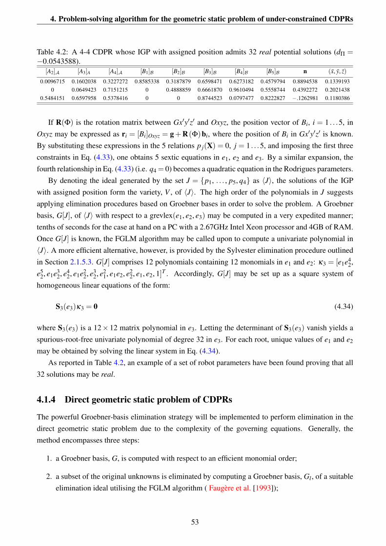
4. Problem-solving algorithm for the geometric static problem of under-constrained CDPRs
Table 4.2: A 4-4 CDPR whose IGP with assigned position admits 32 real potential solutions (dΠ =−0.0543588).
[A2]A [A3]A [A4]A [B1]B [B2]B [B3]B [B4]B [B5]B n (x, y, z)
0.0096715 0.1602038 0.3227272 0.8585338 0.3187879 0.6598471 0.6273182 0.4579794 0.8894538 0.13391930 0.0649423 0.7151215 0 0.4888859 0.6661870 0.9610494 0.5558744 0.4392272 0.2021438
0.5484151 0.6597958 0.5378416 0 0 0.8744523 0.0797477 0.8222827 −.1262981 0.1180386
If R(Φ) is the rotation matrix between Gx′y′z′ and Oxyz, the position vector of Bi, i = 1 . . .5, inOxyz may be expressed as ri = [Bi]Oxyz = g+R(Φ)bi, where the position of Bi in Gx′y′z′ is known.By substituting these expressions in the 5 relations p j(X) = 0, j = 1 . . .5, and imposing the first threeconstraints in Eq. (4.33), one obtains 5 sextic equations in e1, e2 and e3. By a similar expansion, thefourth relationship in Eq. (4.33) (i.e. q4 = 0) becomes a quadratic equation in the Rodrigues parameters.
By denoting the ideal generated by the set J = {p1, . . . , p5, q4} as 〈J〉, the solutions of the IGPwith assigned position form the variety, V , of 〈J〉. The high order of the polynomials in J suggestsapplying elimination procedures based on Groebner bases in order to solve the problem. A Groebnerbasis, G[J], of 〈J〉 with respect to a grevlex(e1, e2, e3) may be computed in a very expedited manner;tenths of seconds for the case at hand on a PC with a 2.67GHz Intel Xeon processor and 4GB of RAM.Once G[J] is known, the FGLM algorithm may be called upon to compute a univariate polynomial in〈J〉. A more efficient alternative, however, is provided by the Sylvester elimination procedure outlinedin Section 2.1.5.3. G[J] comprises 12 polynomials containing 12 monomials in e1 and e2: κ3 = [e1e4
2,e5
2, e1e32, e4
2, e1e22, e3
2, e21, e1e2, e2
2, e1, e2, 1]T . Accordingly, G[J] may be set up as a square system ofhomogeneous linear equations of the form:
S3(e3)κ3 = 0 (4.34)
where S3(e3) is a 12× 12 matrix polynomial in e3. Letting the determinant of S3(e3) vanish yields aspurious-root-free univariate polynomial of degree 32 in e3. For each root, unique values of e1 and e2
may be obtained by solving the linear system in Eq. (4.34).As reported in Table 4.2, an example of a set of robot parameters have been found proving that all
32 solutions may be real.
4.1.4 Direct geometric static problem of CDPRs
The powerful Groebner-basis elimination strategy will be implemented to perform elimination in thedirect geometric static problem due to the complexity of the governing equations. Generally, themethod encompasses three steps:
1. a Groebner basis, G, is computed with respect to an efficient monomial order;
2. a subset of the original unknowns is eliminated by computing a Groebner basis, Gl , of a suitableelimination ideal utilising the FGLM algorithm ( Faugere et al. [1993]);
53

4. Problem-solving algorithm for the geometric static problem of under-constrained CDPRs
3. a least-degree univariate polynomial devoid of extraneous factors is computed by applying anelimination strategy.
For a generic CDPR with n cables, n≤ 6, it so happens that the number of monomials in the unknownvariables, X, comprised in the ideal of the governing equations, J, usually become very high, in theorder of several hundreds. As a consequence, computing a Groebner basis is a nontrivial task. Thefollowing strategy is adopted:
• All geometric parameters of the robot are assigned generic rational values so as to ease numericalcomputation in the computer algebra system, i.e. the GroebnerPackage provided within thesoftware Maple15. Accordingly, 〈J〉 ⊂Q[X], where Q[X] is the set of all polynomials in X withcoefficients in Q.
• Groebner bases are computed with respect to grevlex monomial order.
• The abundance of generators in J plays a key role, since it greatly speeds up the calculation; afeature already noted by Dhingra et al. [2000]). It is therefore fully exploited here within.
By the above expedients, a Groebner basis, G>grevlex [J], of 〈J〉 may generally be computed in afairly expedited way. Once G[J] is known, the normal set, N[J], of 〈J〉; that is, the set of all monomialsthat are not multiples of any leading monomial in G[J], may be easily computed. From the propertiesof Groebner bases (Corless [1996]; Moller [1998]), the number of monomials in N[J] coincides withthe number of complex roots in the variety of 〈J〉 and thus with the number of solutions, Nsol , of theproblem at hand. This is the order of the least-degree univariate polynomials comprised in 〈J〉.
4.1.4.1 Direct geometric static problem of 2-2 CDPRs
The DGP is characterised by assigned values of ρ1 and ρ2 and an unknown platform pose. Consideringx as a linear function of z from the second equation in Eq. (4.6), and substituting into Eq. (4.5) andthe first equation in Eq. (4.6), yields two quadratic equations in z; namely, p4 = 0 and p5 = 0, fromwhich z may be eliminated. By cancelling the nonzero factor, 16(a2x− r21x)
4, a single equation in θ
may further be obtained in the form of p6 = 0. Expressing sθ and cθ as functions of tθ = tan(θ/2) andclearing the factor (1+ t2
θ)6, a 12th-degree polynomial equation in tθ is finally obtained:
12
∑k=0
Bktθ k = 0 (4.35)
As explained by Carricato and Merlet [2013], for each solution of Eq. (4.35), a single value of z iscomputed by the greatest common divisor of p4 and p5, with a single value of x finally obtained fromthe second equation in Eq. (4.6). By considering both operational modes, the problems admits up to24 solutions.
54
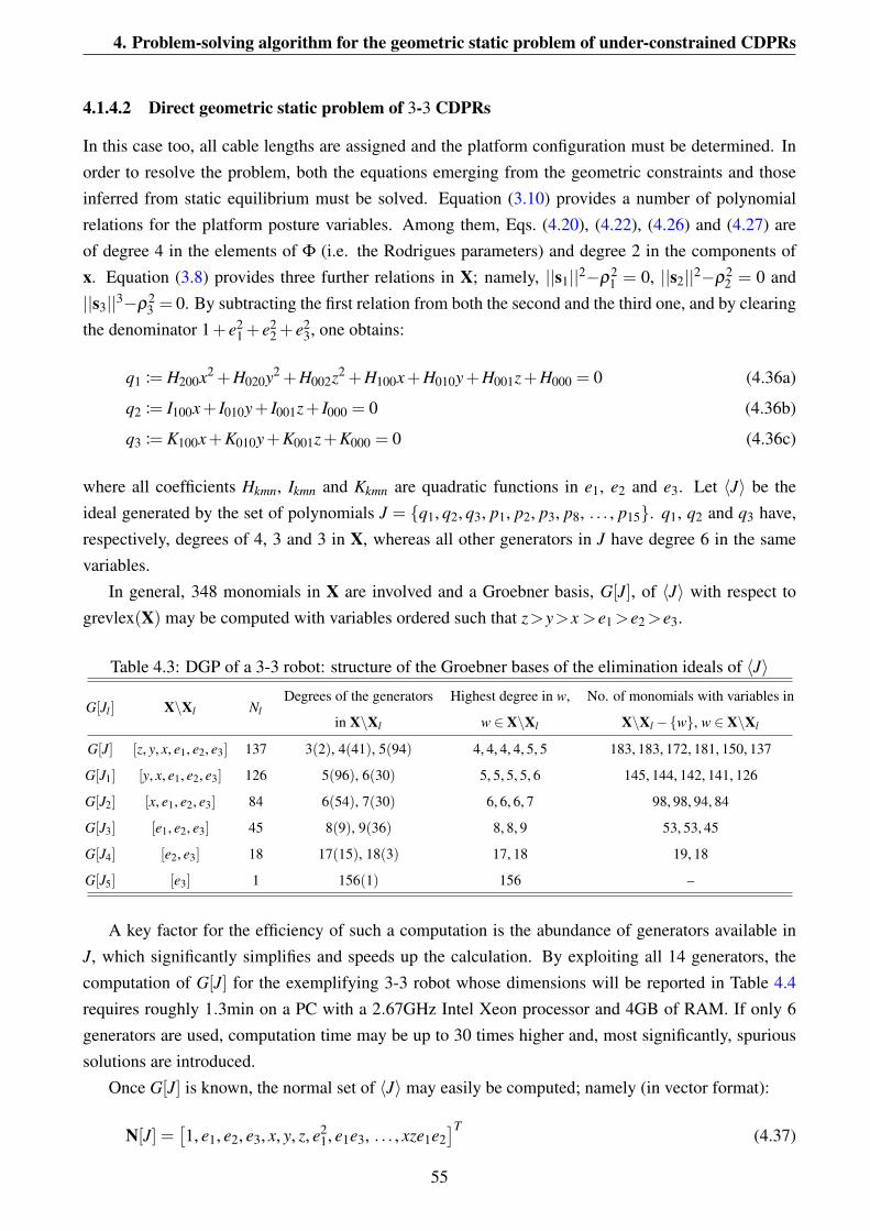
4. Problem-solving algorithm for the geometric static problem of under-constrained CDPRs
4.1.4.2 Direct geometric static problem of 3-3 CDPRs
In this case too, all cable lengths are assigned and the platform configuration must be determined. Inorder to resolve the problem, both the equations emerging from the geometric constraints and thoseinferred from static equilibrium must be solved. Equation (3.10) provides a number of polynomialrelations for the platform posture variables. Among them, Eqs. (4.20), (4.22), (4.26) and (4.27) areof degree 4 in the elements of Φ (i.e. the Rodrigues parameters) and degree 2 in the components ofx. Equation (3.8) provides three further relations in X; namely, ||s1||2−ρ2
1 = 0, ||s2||2−ρ22 = 0 and
||s3||3−ρ23 = 0. By subtracting the first relation from both the second and the third one, and by clearing
the denominator 1+ e21 + e2
2 + e23, one obtains:
q1 := H200x2 +H020y2 +H002z2 +H100x+H010y+H001z+H000 = 0 (4.36a)
q2 := I100x+ I010y+ I001z+ I000 = 0 (4.36b)
q3 := K100x+K010y+K001z+K000 = 0 (4.36c)
where all coefficients Hkmn, Ikmn and Kkmn are quadratic functions in e1, e2 and e3. Let 〈J〉 be theideal generated by the set of polynomials J = {q1, q2, q3, p1, p2, p3, p8, . . . , p15}. q1, q2 and q3 have,respectively, degrees of 4, 3 and 3 in X, whereas all other generators in J have degree 6 in the samevariables.
In general, 348 monomials in X are involved and a Groebner basis, G[J], of 〈J〉 with respect togrevlex(X) may be computed with variables ordered such that z>y>x >e1>e2>e3.
Table 4.3: DGP of a 3-3 robot: structure of the Groebner bases of the elimination ideals of 〈J〉
G[Jl ] X\Xl NlDegrees of the generators Highest degree in w, No. of monomials with variables in
in X\Xl w ∈ X\Xl X\Xl−{w}, w ∈ X\Xl
G[J] [z, y, x, e1, e2, e3] 137 3(2), 4(41), 5(94) 4, 4, 4, 4, 5, 5 183, 183, 172, 181, 150, 137
G[J1] [y, x, e1, e2, e3] 126 5(96), 6(30) 5, 5, 5, 5, 6 145, 144, 142, 141, 126
G[J2] [x, e1, e2, e3] 84 6(54), 7(30) 6, 6, 6, 7 98, 98, 94, 84
G[J3] [e1, e2, e3] 45 8(9), 9(36) 8, 8, 9 53, 53, 45
G[J4] [e2, e3] 18 17(15), 18(3) 17, 18 19, 18
G[J5] [e3] 1 156(1) 156 –
A key factor for the efficiency of such a computation is the abundance of generators available inJ, which significantly simplifies and speeds up the calculation. By exploiting all 14 generators, thecomputation of G[J] for the exemplifying 3-3 robot whose dimensions will be reported in Table 4.4requires roughly 1.3min on a PC with a 2.67GHz Intel Xeon processor and 4GB of RAM. If only 6generators are used, computation time may be up to 30 times higher and, most significantly, spurioussolutions are introduced.
Once G[J] is known, the normal set of 〈J〉 may easily be computed; namely (in vector format):
N[J] =[1, e1, e2, e3, x, y, z, e2
1, e1e3, . . . , xze1e2]T
(4.37)
55
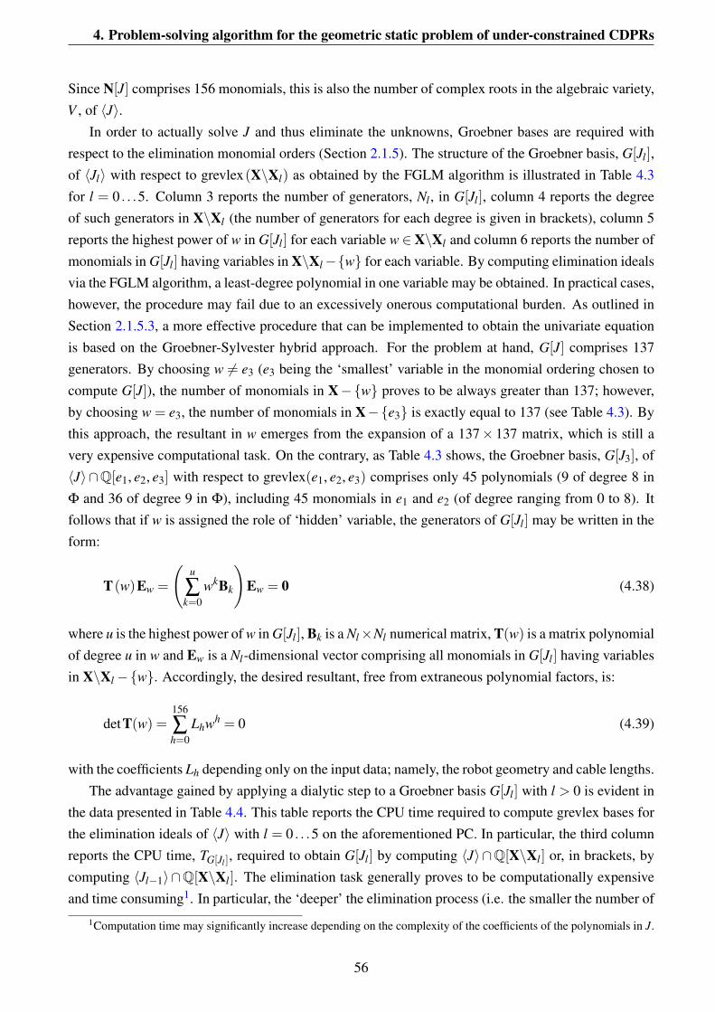
4. Problem-solving algorithm for the geometric static problem of under-constrained CDPRs
Since N[J] comprises 156 monomials, this is also the number of complex roots in the algebraic variety,V , of 〈J〉.
In order to actually solve J and thus eliminate the unknowns, Groebner bases are required withrespect to the elimination monomial orders (Section 2.1.5). The structure of the Groebner basis, G[Jl],of 〈Jl〉 with respect to grevlex(X\Xl) as obtained by the FGLM algorithm is illustrated in Table 4.3for l = 0 . . .5. Column 3 reports the number of generators, Nl , in G[Jl], column 4 reports the degreeof such generators in X\Xl (the number of generators for each degree is given in brackets), column 5reports the highest power of w in G[Jl] for each variable w ∈X\Xl and column 6 reports the number ofmonomials in G[Jl] having variables in X\Xl−{w} for each variable. By computing elimination idealsvia the FGLM algorithm, a least-degree polynomial in one variable may be obtained. In practical cases,however, the procedure may fail due to an excessively onerous computational burden. As outlined inSection 2.1.5.3, a more effective procedure that can be implemented to obtain the univariate equationis based on the Groebner-Sylvester hybrid approach. For the problem at hand, G[J] comprises 137generators. By choosing w 6= e3 (e3 being the ‘smallest’ variable in the monomial ordering chosen tocompute G[J]), the number of monomials in X−{w} proves to be always greater than 137; however,by choosing w = e3, the number of monomials in X−{e3} is exactly equal to 137 (see Table 4.3). Bythis approach, the resultant in w emerges from the expansion of a 137× 137 matrix, which is still avery expensive computational task. On the contrary, as Table 4.3 shows, the Groebner basis, G[J3], of〈J〉∩Q[e1, e2, e3] with respect to grevlex(e1, e2, e3) comprises only 45 polynomials (9 of degree 8 inΦ and 36 of degree 9 in Φ), including 45 monomials in e1 and e2 (of degree ranging from 0 to 8). Itfollows that if w is assigned the role of ‘hidden’ variable, the generators of G[Jl] may be written in theform:
T(w)Ew =
(u
∑k=0
wkBk
)Ew = 0 (4.38)
where u is the highest power of w in G[Jl], Bk is a Nl×Nl numerical matrix, T(w) is a matrix polynomialof degree u in w and Ew is a Nl-dimensional vector comprising all monomials in G[Jl] having variablesin X\Xl−{w}. Accordingly, the desired resultant, free from extraneous polynomial factors, is:
detT(w) =156
∑h=0
Lhwh = 0 (4.39)
with the coefficients Lh depending only on the input data; namely, the robot geometry and cable lengths.The advantage gained by applying a dialytic step to a Groebner basis G[Jl] with l > 0 is evident in
the data presented in Table 4.4. This table reports the CPU time required to compute grevlex bases forthe elimination ideals of 〈J〉 with l = 0 . . .5 on the aforementioned PC. In particular, the third columnreports the CPU time, TG[Jl ], required to obtain G[Jl] by computing 〈J〉∩Q[X\Xl] or, in brackets, bycomputing 〈Jl−1〉∩Q[X\Xl]. The elimination task generally proves to be computationally expensiveand time consuming1. In particular, the ‘deeper’ the elimination process (i.e. the smaller the number of
1Computation time may significantly increase depending on the complexity of the coefficients of the polynomials in J.
56
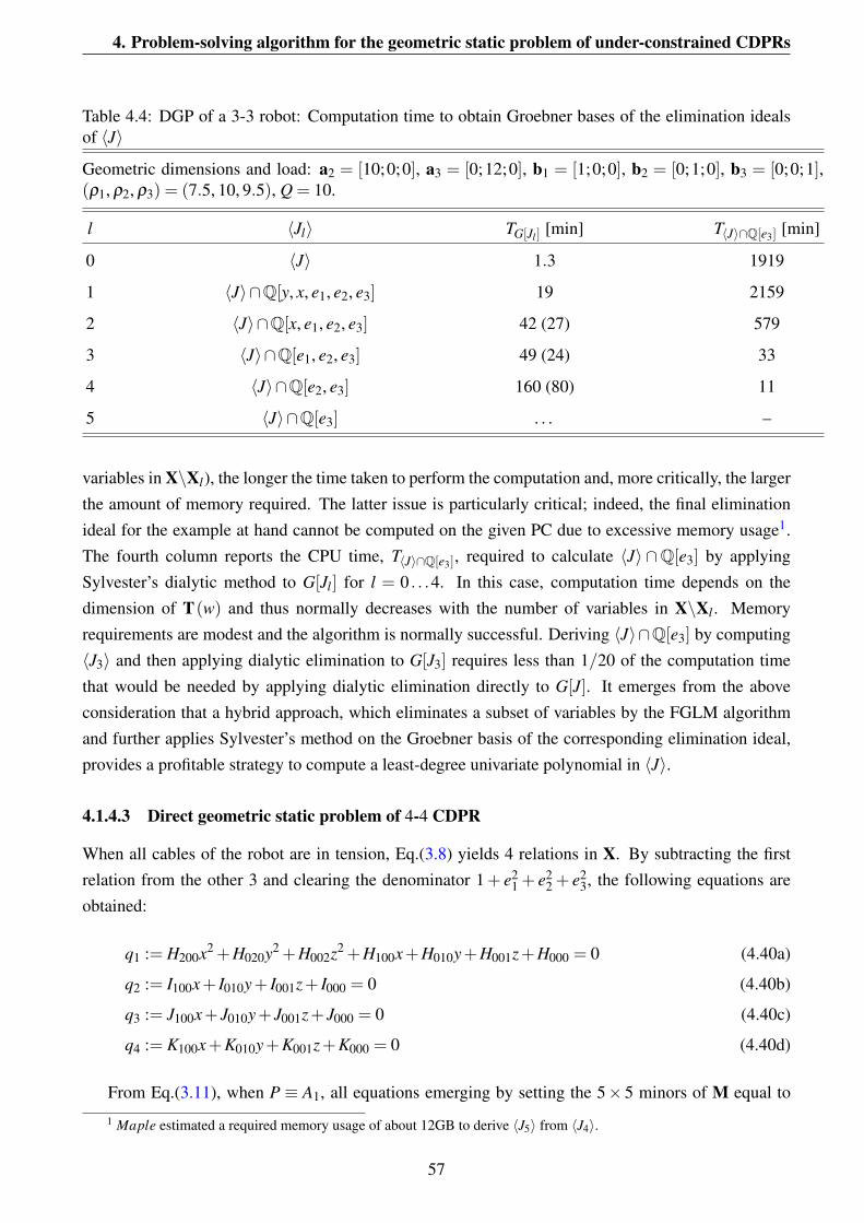
4. Problem-solving algorithm for the geometric static problem of under-constrained CDPRs
Table 4.4: DGP of a 3-3 robot: Computation time to obtain Groebner bases of the elimination idealsof 〈J〉
Geometric dimensions and load: a2 = [10;0;0], a3 = [0;12;0], b1 = [1;0;0], b2 = [0;1;0], b3 = [0;0;1],(ρ1, ρ2, ρ3) = (7.5, 10, 9.5), Q = 10.
l 〈Jl〉 TG[Jl ] [min] T〈J〉∩Q[e3] [min]
0 〈J〉 1.3 1919
1 〈J〉∩Q[y, x, e1, e2, e3] 19 2159
2 〈J〉∩Q[x, e1, e2, e3] 42 (27) 579
3 〈J〉∩Q[e1, e2, e3] 49 (24) 33
4 〈J〉∩Q[e2, e3] 160 (80) 11
5 〈J〉∩Q[e3] . . . –
variables in X\Xl), the longer the time taken to perform the computation and, more critically, the largerthe amount of memory required. The latter issue is particularly critical; indeed, the final eliminationideal for the example at hand cannot be computed on the given PC due to excessive memory usage1.The fourth column reports the CPU time, T〈J〉∩Q[e3], required to calculate 〈J〉 ∩Q[e3] by applyingSylvester’s dialytic method to G[Jl] for l = 0 . . .4. In this case, computation time depends on thedimension of T(w) and thus normally decreases with the number of variables in X\Xl . Memoryrequirements are modest and the algorithm is normally successful. Deriving 〈J〉∩Q[e3] by computing〈J3〉 and then applying dialytic elimination to G[J3] requires less than 1/20 of the computation timethat would be needed by applying dialytic elimination directly to G[J]. It emerges from the aboveconsideration that a hybrid approach, which eliminates a subset of variables by the FGLM algorithmand further applies Sylvester’s method on the Groebner basis of the corresponding elimination ideal,provides a profitable strategy to compute a least-degree univariate polynomial in 〈J〉.
4.1.4.3 Direct geometric static problem of 4-4 CDPR
When all cables of the robot are in tension, Eq.(3.8) yields 4 relations in X. By subtracting the firstrelation from the other 3 and clearing the denominator 1+ e2
1 + e22 + e2
3, the following equations areobtained:
q1 := H200x2 +H020y2 +H002z2 +H100x+H010y+H001z+H000 = 0 (4.40a)
q2 := I100x+ I010y+ I001z+ I000 = 0 (4.40b)
q3 := J100x+ J010y+ J001z+ J000 = 0 (4.40c)
q4 := K100x+K010y+K001z+K000 = 0 (4.40d)
From Eq.(3.11), when P ≡ A1, all equations emerging by setting the 5× 5 minors of M equal to
1 Maple estimated a required memory usage of about 12GB to derive 〈J5〉 from 〈J4〉.
57
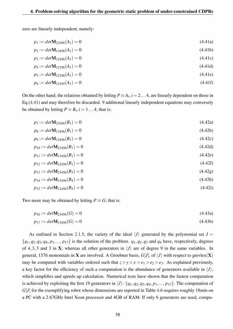
4. Problem-solving algorithm for the geometric static problem of under-constrained CDPRs
zero are linearly independent; namely:
p1 := detM23456(A1) = 0 (4.41a)
p2 := detM13456(A1) = 0 (4.41b)
p3 := detM12456(A1) = 0 (4.41c)
p4 := detM12356(A1) = 0 (4.41d)
p5 := detM12346(A1) = 0 (4.41e)
p6 := detM12345(A1) = 0 (4.41f)
On the other hand, the relations obtained by letting P≡ Ai, i= 2 . . .4, are linearly dependent on those inEq.(4.41) and may therefore be discarded. 9 additional linearly independent equations may converselybe obtained by letting P≡ Bi, i = 1 . . .4; that is:
p7 := detM23456(B1) = 0 (4.42a)
p8 := detM13456(B1) = 0 (4.42b)
p9 := detM12456(B1) = 0 (4.42c)
p10 := detM23456(B1) = 0 (4.42d)
p11 := detM13456(B1) = 0 (4.42e)
p12 := detM12456(B1) = 0 (4.42f)
p13 := detM23456(B3) = 0 (4.42g)
p14 := detM13456(B4) = 0 (4.42h)
p15 := detM12456(B5) = 0 (4.42i)
Two more may be obtained by letting P≡ G; that is:
p16 := detM23456(G) = 0 (4.43a)
p17 := detM13456(G) = 0 (4.43b)
As outlined in Section 2.1.5, the variety of the ideal 〈J〉 generated by the polynomial set J =
{q1, q2, q3, q4, p1, ..., p17} is the solution of the problem. q1, q2, q3 and q4 have, respectively, degreesof 4, 3, 3 and 3 in X; whereas all other generators in 〈J〉 are of degree 9 in the same variables. Ingeneral, 1576 monomials in X are involved. A Groebner basis, G[J], of 〈J〉 with respect to grevlex(X)
may be computed with variables ordered such that z> y> x > e1 > e2 > e3. As explained previously,a key factor for the efficiency of such a computation is the abundance of generators available in 〈J〉,which simplifies and speeds up calculation. Numerical tests have shown that the fastest computationis achieved by exploiting the first 19 generators in 〈J〉: {q1, q2, q3, q4, p1, ..., p17}. The computation ofG[J] for the exemplifying robot whose dimensions are reported in Table 4.6 requires roughly 18min ona PC with a 2.67GHz Intel Xeon processor and 4GB of RAM. If only 6 generators are used, compu-
58

4. Problem-solving algorithm for the geometric static problem of under-constrained CDPRs
tation time is 4 times higher and, most importantly, spurious solutions are introduced as only two outof six minors of M are used. Knowing G[J], the normal set of 〈J〉 may be easily computed; namely (invector format):
N[J] = [1, e3, e2, e1, x, y, z, e23, e2e3, . . . , e1e2e2
3x, e1e2e23y]T (4.44)
Since N[J] comprises 216 polynomials, this is also the number of complex roots (including multiplic-ity) in the algebraic variety, V , of 〈J〉 and thus the order of the least-degree univariate polynomialscomprised in 〈J〉.
The structure of G[J] with respect to grevlex(X), as obtained by the FGLM algorithm, is illustratedin Table 4.5 for l = 0 . . .5. Column 3 reports the number of generators, Nl , in G[Jl], column 4 reportsthe degree of such generators in X\Xl (the number of generators for each degree is given in brackets)and column 5 reports the number of monomials in G[Jl] having variables in X\Xl −{w} for eachvariable w ∈ X\Xl .
As in the 3-cable case, by computing elimination ideals via the FGLM algorithm, a least-degreepolynomial in one variable may be obtained. However, the advantage gained by applying a dialyticstep to a Groebner basis, G[Jl], with l > 0 is evident in the data presented in Table 4.6. The table reportsthe CPU time required to compute grevlex bases for the elimination ideals of 〈J〉 with l = 0 . . .5 onthe aforementioned PC for an exemplifying 4-4 CDPR. In particular, the third column reports the CPUtime, TG[Jl ], required to obtain G[Jl] by computing 〈Jl−1〉∩Q[X\Xl] via the FGLM algorithm and thefourth column reports the CPU time, T〈J〉∩Q[e3], required to calculate 〈J〉∩Q[e3] via application ofdialytic elimination to G[Jl] for l = 0 . . .4. As expected, the higher l is (i.e. the more variables areeliminated), the more demanding the FGLM elimination becomes. In particular, the last eliminationideal cannot be computed due to excessive memory usage. Conversely, the computation time of thedialytic step decreases with l, as it depends on the dimensions of T(w). For the example at hand,〈J〉∩Q[e3] cannot be computed from G[Jl] with l = 0 . . .2 due to excessive computation time. Instead,the univariate polynomial in e3 may be successfully computed from either G[J3] or G[J4]. The moreefficient computation of 〈J〉∩Q[e3] is obtained by eliminating {x, y, z} by the FGLM algorithm and{e1, e2} by the dialytic step.
4.1.4.4 Direct geometric static problem of 5-5 CDPRs
Solutions to the DGP of a robot with 5 cables and the corresponding univariate polynomial are com-puted by implementing the same elimination strategy. From Eq. (3.8), 5 polynomials may be derived;namely, {qi, i = 1 . . .5}, similar to Eq. (4.40). For the case of 5-5 CDPRs, M is a 6× 6 matrix fromwhich only one equation is obtained by letting its determinant equal zero:
p := detM(A1) = 0 (4.45)
In contrast to the cases of robots with n < 5 cables, all other similar relations obtained by changing thereduction pole of the moment linearly depend on Eq.(4.45) and must therefore be discarded. Thus, in
59

4. Problem-solving algorithm for the geometric static problem of under-constrained CDPRs
Table 4.5: Structure of the Groebner bases of the elimination ideals of 4-4 CDPRs
G[Jl] X\Xl NlDegrees of the generators No. of monomials with variables in
in X\Xl X\Xl−{w}, w ∈ X\Xl
G[J] [z, y, x, e1, e2, e3] 195 3(3), 4(5), 5(158), 6(29) 230, 232, 232, 271, 224, 195
G[J1] [y, x, e1, e2, e3] 147 5(36), 6(111) 185, 180, 181, 160, 147
G[J2] [x, e1, e2, e3] 111 5(1), 7(99), 8(11) 127, 127, 117, 111
G[J3] [e1, e2, e3] 61 8(1), 10(60) 66, 61, 61
G[J4] [e2, e3] 21 20(15), 21(6) 22, 21
G[J5] [e3] 1 216(1) –
Table 4.6: Computation times to obtain Groebner bases of the elimination ideals of 4-4 CDPRs for therobot geometry :a1 = [0;0;0], a2 = [9;0;1], a3 = [11;9;0], a4 = [−2;8;−1], b1 = [−2;−1;−1], b2 =[1;−2;0], b3 = [2;1;−1], b4 = [0;2;−1], (ρ1, ρ2, ρ3, ρ4) = (6, 7, 8, 9), Q = 10.
l 〈Jl〉 TG[Jl ] [min] T〈J〉∩Q[e3] [min]
0 〈J〉 17 . . .
1 〈J〉∩Q[y, x, e1, e2, e3] 227 . . .
2 〈J〉∩Q[x, e1, e2, e3] 670 . . .
3 〈J〉∩Q[e1, e2, e3] 567 340
4 〈J〉∩Q[e2, e3] 1063 67
5 〈J〉∩Q[e3] . . . –
this case the ideal, 〈J〉, comprises just 6 polynomials, {q1, q2, q3, q4, q5, p}, in which q1, q2, q3, q4 andq5 have, respectively, degrees of 4, 3, 3, 3 and 3 in X while p, inferred from static equilibrium, has adegree as high as 9 in the same variables. The total number of monomials in X contained in 〈J〉 is 1576.Though the computation of G[J] may not take advantage of redundant generators in J, it is relativelyfast, mainly due to the fact that a single high-degree polynomial appears in J. For the exemplifyingrobot reported in subsequent Table 4.8, G[J] may be computed in roughly 3 minutes.
The normal set; namely:
N[J] = [1, e3, e2, e1, x, y, z, e23, e2e3, . . . , e1xy2, e1xyz, x4]T (4.46)
contains 140 monomials such that Nsol = 140. The structure of G[Jl] with respect to grevlex(X\Xl)
is reported in Table 4.7 for l = 0 . . .5. The table is constructed in the same manner as Table 4.5.Notably, in this case, G[Jl] comprises monomials in X\Xl −{e3} equal to Nl for only l = 1, 3, 4.Hence, Sylvester dialytic elimination may be applied to neither G[J] nor G[J2]. Indeed, these containmore monomials in X\Xl−{e3} than available generators.
Table 4.8 reports, for an exemplifying generic robot, the CPU time, TG[Jl ], required to compute
60
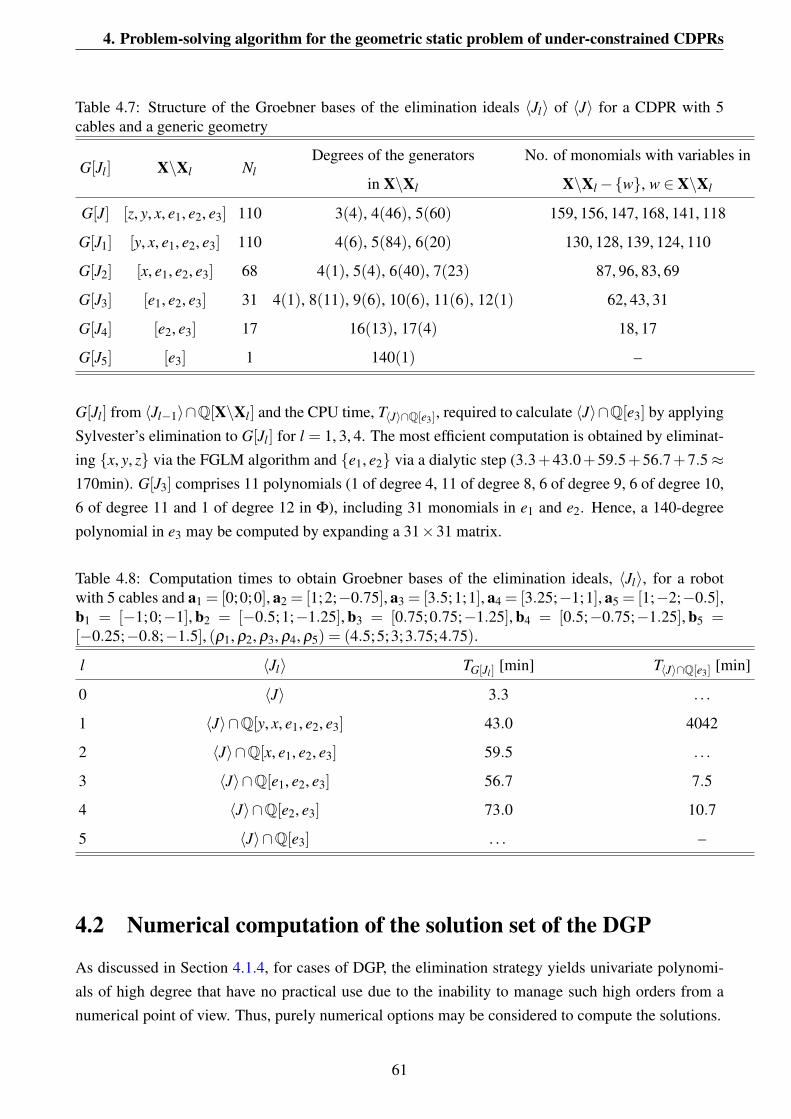
4. Problem-solving algorithm for the geometric static problem of under-constrained CDPRs
Table 4.7: Structure of the Groebner bases of the elimination ideals 〈Jl〉 of 〈J〉 for a CDPR with 5cables and a generic geometry
G[Jl] X\Xl NlDegrees of the generators No. of monomials with variables in
in X\Xl X\Xl−{w}, w ∈ X\Xl
G[J] [z, y, x, e1, e2, e3] 110 3(4), 4(46), 5(60) 159, 156, 147, 168, 141, 118
G[J1] [y, x, e1, e2, e3] 110 4(6), 5(84), 6(20) 130, 128, 139, 124, 110
G[J2] [x, e1, e2, e3] 68 4(1), 5(4), 6(40), 7(23) 87, 96, 83, 69
G[J3] [e1, e2, e3] 31 4(1), 8(11), 9(6), 10(6), 11(6), 12(1) 62, 43, 31
G[J4] [e2, e3] 17 16(13), 17(4) 18, 17
G[J5] [e3] 1 140(1) –
G[Jl] from 〈Jl−1〉∩Q[X\Xl] and the CPU time, T〈J〉∩Q[e3], required to calculate 〈J〉∩Q[e3] by applyingSylvester’s elimination to G[Jl] for l = 1, 3, 4. The most efficient computation is obtained by eliminat-ing {x, y, z} via the FGLM algorithm and {e1, e2} via a dialytic step (3.3+43.0+59.5+56.7+7.5≈170min). G[J3] comprises 11 polynomials (1 of degree 4, 11 of degree 8, 6 of degree 9, 6 of degree 10,6 of degree 11 and 1 of degree 12 in Φ), including 31 monomials in e1 and e2. Hence, a 140-degreepolynomial in e3 may be computed by expanding a 31×31 matrix.
Table 4.8: Computation times to obtain Groebner bases of the elimination ideals, 〈Jl〉, for a robotwith 5 cables and a1 = [0;0;0], a2 = [1;2;−0.75], a3 = [3.5;1;1], a4 = [3.25;−1;1], a5 = [1;−2;−0.5],b1 = [−1;0;−1], b2 = [−0.5;1;−1.25], b3 = [0.75;0.75;−1.25], b4 = [0.5;−0.75;−1.25], b5 =[−0.25;−0.8;−1.5], (ρ1, ρ2, ρ3, ρ4, ρ5) = (4.5;5;3;3.75;4.75).
l 〈Jl〉 TG[Jl ] [min] T〈J〉∩Q[e3] [min]
0 〈J〉 3.3 . . .
1 〈J〉∩Q[y, x, e1, e2, e3] 43.0 4042
2 〈J〉∩Q[x, e1, e2, e3] 59.5 . . .
3 〈J〉∩Q[e1, e2, e3] 56.7 7.5
4 〈J〉∩Q[e2, e3] 73.0 10.7
5 〈J〉∩Q[e3] . . . –
4.2 Numerical computation of the solution set of the DGP
As discussed in Section 4.1.4, for cases of DGP, the elimination strategy yields univariate polynomi-als of high degree that have no practical use due to the inability to manage such high orders from anumerical point of view. Thus, purely numerical options may be considered to compute the solutions.
61

4. Problem-solving algorithm for the geometric static problem of under-constrained CDPRs
4.2.1 Eigenvalue formulation
As discussed in Section 2.1.5.2, once a Groebner basis, G[J], of 〈J〉 is known, the solutions of theproblem may be efficiently computed by constructing a multiplication matrix with the eigenproblemmethod in Eq. (2.11). Considering N[J] from Eqs. (4.37), (4.44) and (4.46) for the cases of robots with3, 4 and 5 cables, one may identify that the first 7 entries of N[J] are always 1, e1, e2, e3, x, y, z. Foreach case, a unique solution in X emerges from each eigenvector, Ni, as:
e1, i =ti, 2
ti, 1, e2, i =
ti, 3
ti, 1, e3, i =
ti, 4
ti, 1, xi =
ti, 5
ti, 1yi =
ti, 6
ti, 1, zi =
ti, 7
ti, 1. (4.47)
For all cases, computation of A[J, e3] and the corresponding eigenvalues may be performed in tenthsof a second. Once a robot configuration is found, cable tensions may be obtained via any subset ofEq. 3.9. A drawback of this approach is that it relies on a prior computation of G[J]. The efficiency ofGroebner basis computation depends heavily on the ‘size’ of the rational coefficients of the polynomialsgenerating the basis. Indeed, for Groebner-basis computation, the coefficients expressing the robotgeometric parameters must be assigned rational values, which are normally obtained by converting realvalues. The higher the number of digits in the original floating-point data, the larger the numeratorsand denominators of the resulting rationals and the larger the coefficients in the polynomials formingthe ideal. As a result, computation becomes slower and more memory-demanding. This is a limitationshared by all computational methods using Groebner bases.
4.2.2 Homotopy continuation
Due to the drawbacks of the eigenvalue formulation discussed in the previous section, homotopy con-tinuation (Sommese and Wampler [2005]) is chosen to compute the solution set numerically. Continu-ation has the significant advantage that it requires no prior Groebner-basis computation by a computeralgebra system and real-value geometric parameters may be directly handled with floating-point arith-metic. As a consequence, the dependence of computation time on the specific values of the robotparameters is rather modest.
Though formulating equilibrium constraints via Eq. (3.11) is particularly favourable when pursuingelimination strategies, the complexity and high degree of the polynomials emerging from the elimina-tion of cable tensions are a disadvantage for continuation algorithms, as they slow down computationand cause stability problems. For this reason, formulation via Eqs. (3.8) and (3.9) is preferable. Forthe same reason, pose parameterisation by Study or Dietmaier coordinates (see Sections 3.3 and 3.4) ispreferable over the 6-parameter representation described in Section 3.2. Though the resulting systeminvolves more variables and more equations than that in the elimination strategy, it comprises muchsimpler lower-order polynomials, which are more stable when homotopy continuation is implemented,thus leading to faster computation.
62
4. Problem-solving algorithm for the geometric static problem of under-constrained CDPRs
4.2.2.1 General homotopy continuation
As introduced in Section 2.2, polynomial homotopy continuation is a path-tracking technique thattransforms a start system of polynomial equations with known solutions to a target system whosesolutions must be found (Sommese and Wampler [2005]). The method tracks the evolution of a systemsuch as:
H(Y, t) = γ (1− t)F0 (Y)+ tF1 (Y) = 0 (4.48)
where F0 (Y) and F1 (Y) are the start and the target system, respectively, γ is a randomly selectedcomplex number and t is a real number called the continuation parameter. The concept consists ofvarying t from 0 to 1 while tracking the solutions of the problem from those of F0 (Y) = 0, known, tothose of F1 (Y) = 0, unknown.
As previously discussed, the procedure may be classified as general homotopy continuation orparameter homotopy continuation depending on how the start system is constructed. The former isemployed when no information is known a priori about the roots of the target system. In this case, astart system yielding the maximum possible number of solutions must be constructed. This number isequal to the minimum multi-homogeneous Bezout number, NBez, of the target system (Wampler et al.[1990]). Since NBez coincides with the number of paths to be tracked, it is of paramount importancefor computational efficiency.
In the case of a robot with 2 cables, one may take advantage of in-plane formulation by ignoringall variables corresponding to direction j. Accordingly, the attachment points on the base and movingplatform may be expressed as:
[A1]O = [0, 0, 0]T , [A2]O = [a21, 0, a23]T , [B1]O′ = [b11, 0, 0]T , [B2]O′ = [b21, 0, 0]T ,
[G]O = [x, 0, z]T(4.49)
Using Dietmaier parameterisation, having x = [x, 0, z]T and altering the components of e1 and e2 to:
e1 = [e11, 0, e13]T , e2 = [e21, 0, e23]
T (4.50)
the position vectors of points B1, B2 and G in Oxz may be written as functions of 6 variables:
X = [x, z, e11, e13, e21, e23]T (4.51)
Using this parameterisation, 2 geometric equations from Eq. (3.8) and 3 equilibrium equations fromEq. 3.9 may be derived. By introducing the 3 equations from Eq. (3.19), a system of 8 polynomialsin 8 variables (X, τ1 and τ2) is obtained, which governs the DGP of a 2-2 CDPR in the x-z plane. Asoutlined in Section 2.2.1, when considering general homotopy continuation, a start system must beconstructed with the number of solutions equal to the minimum multi-homogeneous Bezout number.For the case at hand, using the multi-homogenisation {τ1, τ2}, {e11, e13, e21, e23, x, z} yields a minimumBezout number of 96.
63
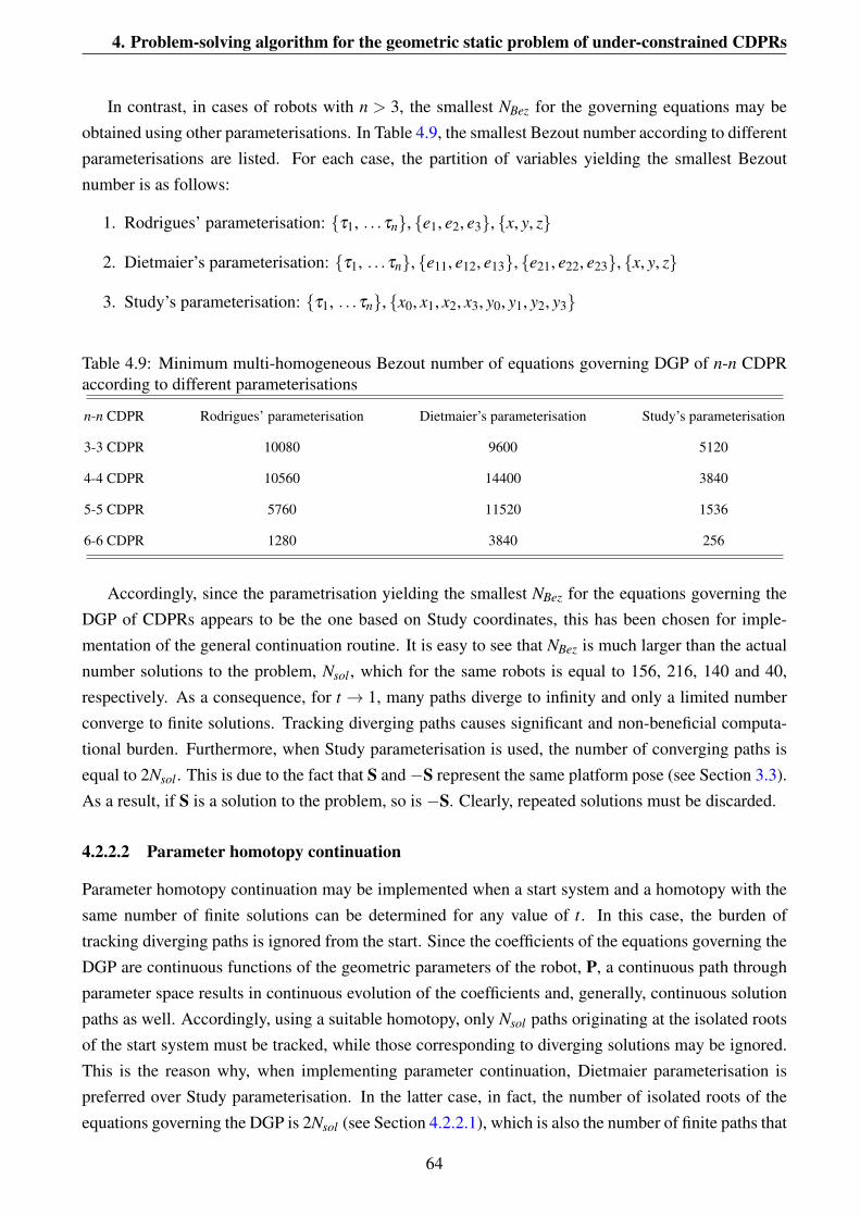
4. Problem-solving algorithm for the geometric static problem of under-constrained CDPRs
In contrast, in cases of robots with n > 3, the smallest NBez for the governing equations may beobtained using other parameterisations. In Table 4.9, the smallest Bezout number according to differentparameterisations are listed. For each case, the partition of variables yielding the smallest Bezoutnumber is as follows:
1. Rodrigues’ parameterisation: {τ1, . . .τn}, {e1, e2, e3}, {x, y, z}
2. Dietmaier’s parameterisation: {τ1, . . .τn}, {e11, e12, e13}, {e21, e22, e23}, {x, y, z}
3. Study’s parameterisation: {τ1, . . .τn}, {x0, x1, x2, x3, y0, y1, y2, y3}
Table 4.9: Minimum multi-homogeneous Bezout number of equations governing DGP of n-n CDPRaccording to different parameterisations
n-n CDPR Rodrigues’ parameterisation Dietmaier’s parameterisation Study’s parameterisation
3-3 CDPR 10080 9600 5120
4-4 CDPR 10560 14400 3840
5-5 CDPR 5760 11520 1536
6-6 CDPR 1280 3840 256
Accordingly, since the parametrisation yielding the smallest NBez for the equations governing theDGP of CDPRs appears to be the one based on Study coordinates, this has been chosen for imple-mentation of the general continuation routine. It is easy to see that NBez is much larger than the actualnumber solutions to the problem, Nsol , which for the same robots is equal to 156, 216, 140 and 40,respectively. As a consequence, for t → 1, many paths diverge to infinity and only a limited numberconverge to finite solutions. Tracking diverging paths causes significant and non-beneficial computa-tional burden. Furthermore, when Study parameterisation is used, the number of converging paths isequal to 2Nsol . This is due to the fact that S and−S represent the same platform pose (see Section 3.3).As a result, if S is a solution to the problem, so is −S. Clearly, repeated solutions must be discarded.
4.2.2.2 Parameter homotopy continuation
Parameter homotopy continuation may be implemented when a start system and a homotopy with thesame number of finite solutions can be determined for any value of t. In this case, the burden oftracking diverging paths is ignored from the start. Since the coefficients of the equations governing theDGP are continuous functions of the geometric parameters of the robot, P, a continuous path throughparameter space results in continuous evolution of the coefficients and, generally, continuous solutionpaths as well. Accordingly, using a suitable homotopy, only Nsol paths originating at the isolated rootsof the start system must be tracked, while those corresponding to diverging solutions may be ignored.This is the reason why, when implementing parameter continuation, Dietmaier parameterisation ispreferred over Study parameterisation. In the latter case, in fact, the number of isolated roots of theequations governing the DGP is 2Nsol (see Section 4.2.2.1), which is also the number of finite paths that
64
4. Problem-solving algorithm for the geometric static problem of under-constrained CDPRs
must be tracked for parameter homotopy to work in a robust manner. This problem does not appearif Dietmaier parameterisation is used, as in this case the number of isolated roots of the modellingequations is exactly Nsol .
When Nsol isolated roots are known for a generic P = P0, the solutions for any other P = P1 maybe found by tracking the homotopy:
F(Y, (1− t)P0 + tP1) = 0 (4.52)
with t varying from 0 to 1 or, more robustly, along the curve t = γt ′/[1+(γ−1)t ′], with t ′ ∈ [0, 1] andγ ∈ C.
4.3 Number of real-valued solutions of the DGP
As outlined previously, the solution strategies introduced for solving the systems of equations govern-ing the displacement analysis of under-constrained CDPRs provide all solutions to the problems in thecomplex field. As a matter of fact, the number of solutions, Nsol , may be complex or real; however,only the latter are of physical interest. By varying robot parameters, the number of real roots varies.Since there may be roots that always remain complex in the solution set, the maximum number of realsolutions in each case may be less than Nsol . Determining a tight bound on this number is a challeng-ing task. In the DGP of under-constrained CDPRs, the upper bound on the number of solutions in thecomplex field was 24, 156, 216 and 140 for robots with 2, 3, 4 and 5 cables, respectively. Except in thecase of a 2-2 CDPR, where a robot parameter set was obtained randomly with all 24 solutions beingreal, there is usually no knowledge of the maximum number of real solutions that may be obtained fora particular parameter set. Due to the very high number of solutions, it is almost impossible to find arobot parameter set with all such solutions being real. It is therefore necessary to use a systematic pro-cedure for finding parameters with the maximum number of real solutions. Accordingly, the Dietmaierprocedure introduced in Section 2.3 may be implemented to find sets of CDPR parameters for whichthe DGP provides the highest number of real configurations. The algorithm begins with a system ofequations with known solutions and proceeds by iteratively changing the parameters in such a way thattwo complex conjugate solutions become continually nearer until they transform into a double real rootand, thereafter, a pair of distinct real solutions. This is achieved by decrementing the absolute value ofthe imaginary parts of the two complex conjugate solutions in question. The procedure is repeated forall pairs of complex conjugate roots until the maximum number of real solutions is obtained. To im-plement the algorithm successfully, the governing equations of the problem must first be re-derived bychoosing an appropriate coordinate system and applying a suitable parameterisation. More explanationon how the equations are derived is provided in the following sections.
65

4. Problem-solving algorithm for the geometric static problem of under-constrained CDPRs
4.3.1 Governing equations and parameterisation
It has been shown that, for each solution strategy, the equations governing the DGP may becomesimpler by adopting a suitable parameterisation and choosing an appropriate coordinate system. Forexample, Rodriques’ parameterisation with the least number of variables is suitable for eliminationstrategies, while Study’s and Dietmaier parameterisation are the most suitable procedures for numer-ical methods. Further to parameterisation, the proper definition of geometric parameters has greatimportance if the algorithm is to work efficiently. Here, the equations governing the DGP of a robotare re-derived by choosing appropriate coordinate axes and reference points. The origin of the Carte-sian frame appended to the moving platform, O′x′y′z′, is chosen to coincide with B1 such that theposition of the moving platform with respect to the base is described by the vector n, identifying theposition of point B1 instead of the centre of mass, G. By this choice, the position vectors of pointsB1, B2, . . . , Bn, and G on frame B may be expressed as:
[B1]O′ = [0, 0, 0]T , [B2]O′ = [b21, 0, 0]T , [B3]O′ = [b31, b32, 0]T ,...
[Bn]O′ = [bn1, bn2, bn3]T ,
[G]O′ = [g1, g2, g3]T
(4.53)
As discussed in Section 2.3, the algorithm is mainly based on the definition of two scalar functions, Sh
and Drs, that measure the ‘distance’ between either a pair of complex conjugate solutions or two realroots. Since the solutions of the DGP, are vectors, any definition of such functions requires appropri-ate weighting of the vector components. This is difficult to accomplish, however, since the solutionvectors are dimensionally non-homogeneous. The non-homogeneity of solutions is due to the factthat they comprise variables corresponding to cable tensions. Parameterisation can also cause non-homogeneity. For example, as discussed in Section 3.2, Rodrigues parameterisation gives solutions ofmixed dimensions. Those of Φ = (e1 : e2 : e3) are dimensionless, while parameters in x correspondingto the position of the moving platform have dimensions of length. The problem of non-homogeneitymay be circumvented by firstly changing the parameterisation. As discussed in Section 3.4, Dietmaierparameterisation provides all posture parameters of the moving platform with the same dimensions oflength, which makes it appropriate for defining the scalar functions in the algorithm. Additionally, byobserving that a unique solution for the cable tensions, τ , corresponds to any given equilibrium pose,X, the cable tension variables may be ignored in the aforementioned definition. Accordingly, distancefunctions may be equivalently defined in the platform configuration space, which is dimensionallyhomogeneous1.
By implementing Dietmaier parameterisation and scaling the robot such that ρ1 = 1, the positionvector n = B1− A1 has unit magnitude2. Eqs. (3.8), (3.9) and (3.19) yield a system of equations,
1 Indeed, the solutions of the DGP may be computed directly in terms of X by way of Eqs. (3.8) and (3.11).2 This is somewhat equivalent to establishing a ‘characteristic’ length for the Euclidean group of rigid-body displace-
ments. The operation is generally physically inconsistent, but it is not so in this case, as ρ1 is an assigned constant.
66
4. Problem-solving algorithm for the geometric static problem of under-constrained CDPRs
F(Y, P) = 0, in which Y and P are defined as follows:
P = [ρ2, ρ3, . . .ρn,
a21, a23, a31, a32, a33, . . . , an1, an2, an3,
b21, b31, b32, . . .bn1, bn2, bn3,
g1, g2, . . .gn]T
(4.54)
Y =[XT , τ
T ]T = [n1, n2, n3, e11, e12, e13, e21, e22, e23, τ1, τ2, . . .τn]T (4.55)
4.3.2 Application of the Dietmaier algorithm
The start system is easily constructed by choosing an arbitrary set, P0, of geometric parameters andcomputing the corresponding solution set by homotopy continuation. From Eq. (2.29), the incrementof a complex solution, Y, according to a change in P, may be obtained as:
AdP+BdY = 0 (4.56)
The dimensions of matrices A and B vary depending on the number of cables in each CDPR case. Forexample, for a robot with 3 cables, the system of equations F(Y, P) comprises 12 equations for 12unknown variables, Y, and 13 geometric parameters, P. Accordingly, the size of matrices A and B are12×13 and 12×12, respectively. From Eq. 2.31, the increment of Y may be computed as:
dY =−B−1AdP (4.57)
Since the last n rows of matrix −B−1A for CDPRs relate the increment of cable tensions to changes inP, they may be eliminated from the matrix −B−1A. Calling this new matrix J, dX may be computedas:
dX = JdP (4.58)
and thus:
dXh = JhdP (4.59)
where Jh is matrix J evaluated for Y = Yh.An alternative procedure consists of choosing relations within Eq. (3.11) and complementing them
with Eqs. (3.8) and (3.19), thus obtaining an alternative system of 9 equations that depend only on the9 platform coordinates and the geometric parameters; namely:
F′ (X, P) =[
f ′1 (X, P) , . . . , f ′9 (X, P)]T
= 0 (4.60)
67

4. Problem-solving algorithm for the geometric static problem of under-constrained CDPRs
By differentiating Eq. (4.60), one obtains an alternative formulation, J′h, of Jh. Indeed, by choos-ing different triplets of equations within Eq. (3.11), one may obtain several alternative formulationsof Jh. Switching between Jh and any other substitute Jacobian, J′h, may prove useful when Jh isill-conditioned, in order to smooth the numerical computation. By the above observation, the minimi-sation and maximisation procedure formulated in Eq. (2.38) and Eq. (2.39) may be redefined accordingto the corresponding pose, Xh, as:
minimize : sgn[Im(XT
h
)]Im(Jh)∆P
subject to : −∆Pmax ≤ ∆P≤ ∆Pmax;(Xr−Xs)
T (Jr−Js)∆P≥ 0, ∀(Xr, Xs) : Drs < Dmin
(4.61)
and:
maximize : (Xu−Xv)T (Ju−Jv)∆P
subject to : −∆Pmax ≤ ∆P≤ ∆Pmax;(Xr−Xs)
T (Jr−Js)∆P≥ 0, ∀(Xr, Xs) : Drs < Dmin
(4.62)
At this point, the optimisation procedures may be performed efficiently. It may happen that theoptimisation procedure fails, returning ∆P = 0 for Sh > ε . In this case, the algorithm attempts to ad-vance by improving the accuracy with which the solution path is tracked (achieved by decreasing ∆Pmax
or switching between different formulations of the DGP equations) or by relaxing the constraints inEq. (2.38) (i.e. decreasing Dmin to allowing real solutions to become closer). By finding an incre-ment, ∆P, the set of geometric parameters is updated and the solutions of the modified F(Y, P) arethen computed by help of an iterative Newton-Raphson routine. If the Newton-Raphson routine doesnot converge or converges twice to the same solution (likely to occur when the paths corresponding totwo distinct solutions pass close to each other), a different start guess is attempted (i.e. Xh) or a dif-ferent formulation of the DGP equations is utilised. If the Newton-Raphson routine continues to fail,the solution set is updated by a more robust, but slower, solver; namely, a parameter-homotopy-basedroutine implemented within Bertini Bates et al.. At any iteration step, the algorithm works on thepair of complex conjugate solutions whose mutual distance is the shortest. The general structure of thealgorithm is presented in Tab. 4.3.2.
4.3.2.1 Auxiliary parameters of the algorithm
The effectiveness and efficiency of Dietmaier’s algorithm depends on the proper adjustment of a num-ber of auxiliary parameters. A brief discussion concerning the most important ones is presented in thefollowing section.
∆Pmax : The smaller ∆Pmax, the slower the advancement of the algorithm, but the better the lineari-sation approximation in procedures (2.38) and (2.39) and, thus, the more accurate the obtained results.A reasonable strategy consists of choosing a not-too-small increment at the beginning of each iteration(e.g. ∆Pmax = 0.01). Subsequently, if the optimisation step is successful and the imposed constraintsare respected after P and X are updated, the value of ∆Pmax is considered acceptable; otherwise, it is
68
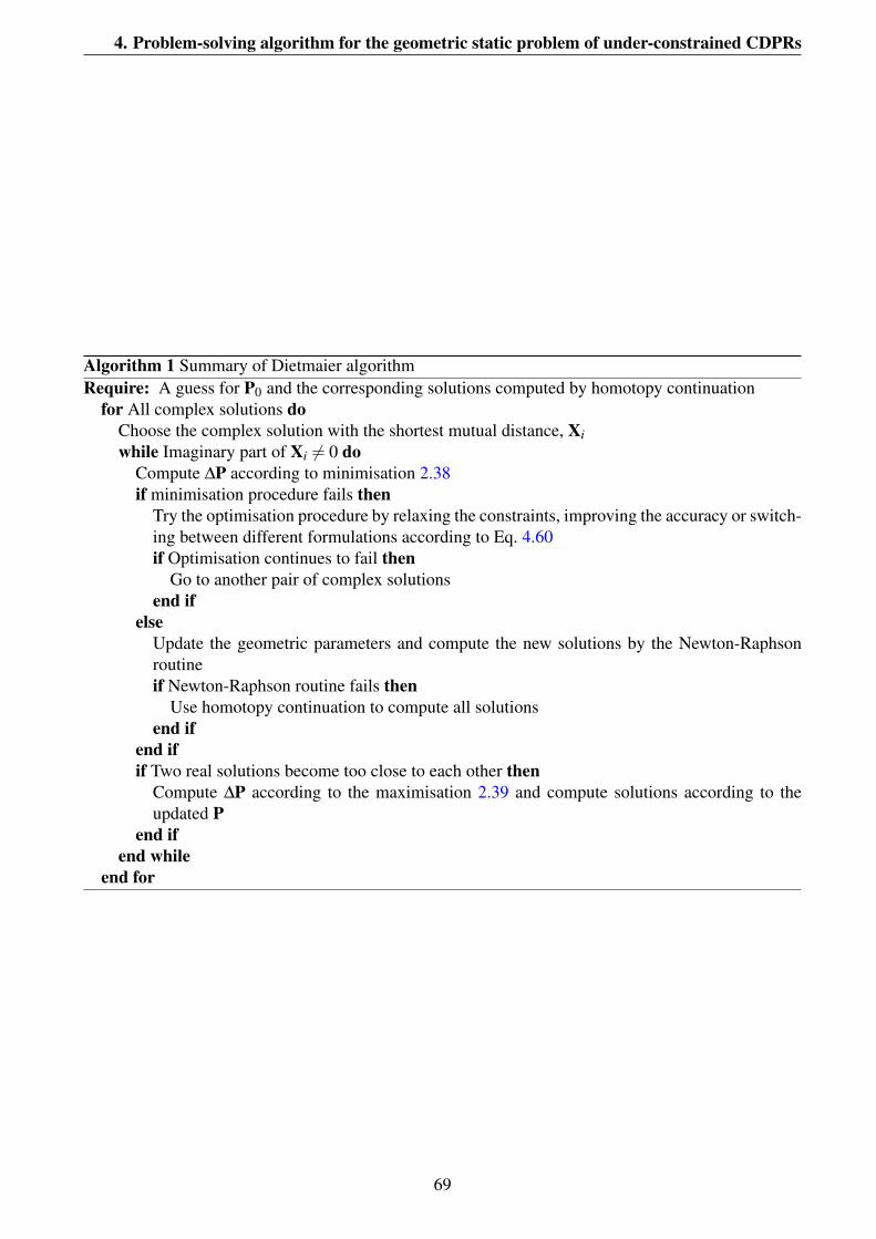
4. Problem-solving algorithm for the geometric static problem of under-constrained CDPRs
Algorithm 1 Summary of Dietmaier algorithmRequire: A guess for P0 and the corresponding solutions computed by homotopy continuation
for All complex solutions doChoose the complex solution with the shortest mutual distance, Xiwhile Imaginary part of Xi 6= 0 do
Compute ∆P according to minimisation 2.38if minimisation procedure fails then
Try the optimisation procedure by relaxing the constraints, improving the accuracy or switch-ing between different formulations according to Eq. 4.60if Optimisation continues to fail then
Go to another pair of complex solutionsend if
elseUpdate the geometric parameters and compute the new solutions by the Newton-Raphsonroutineif Newton-Raphson routine fails then
Use homotopy continuation to compute all solutionsend if
end ifif Two real solutions become too close to each other then
Compute ∆P according to the maximisation 2.39 and compute solutions according to theupdated P
end ifend while
end for
69
4. Problem-solving algorithm for the geometric static problem of under-constrained CDPRs
decreased. For instance, when the minimisation (2.38) is attempted, ∆Pmax is decreased when either∆P = 0 (i.e. the minimisation algorithm fails) or a nonzero ∆P is found but, after P and X are updated,Dh is verified to not decrease or the number of real solutions is lower.
Dmin : The smaller this parameter, the weaker the imposed constraints on the optimisation routinesand, thus, the likelier the routines are to be successful. When Dmin is small, however, real solutionsare allowed to become closer together and the risk of two becoming a complex conjugate is higher.Accordingly, at the beginning of each iteration, Dmin is set equal to a given fraction (e.g. 1/6) of theaverage distance between all real solutions. Subsequently, if optimisation fails, Dmin is decreased (i.e.constraints are relaxed); whereas, if a pair of real solutions switches back to the complex domain, Dmin
is increased.ε : This parameter should be chosen, in theory, small enough to make, from a numerical point
of view, both(Xh, Xh
)∈ C9×C9 and (Xu, Xv) ∈ R9×R9 satisfy F(Y, P) = 0. Setting ε too small,
however, would significantly slow the process. As a rule of thumb, experiments have shown that ε isnot required to be smaller than e−4.
4.3.2.2 Case study
The program has been repeatedly executed with different start systems and parameter-tuning configura-tions for CDPRs with 3, 4 and 5 cables. Accordingly, the maximum number of real solutions obtainedfor each case is 54, 98 and 74, respectively. An example of the corresponding parameters is as follows:
1. Example of 3-3 CDPR parameters with maximum number of 54 real equilibrium configurations:a1 = [0, 0, 0],a2 = [0.89744, 0, −0.72651],a3 = [0.65671, 0.74636, −0.59091], b1 = [1.55665, 0,0], b2 = [0.69695, 0.78429, 0], b3 = [−0.46441, −1.38980, −1.19948], (ρ1, ρ2, ρ3)= (1, 1.0805,2.6025) and Q = 10.
2. Example of 4-4 CDPR parameters with maximum number of 98 real equilibrium configurations:a1 = [5.521454, 7.836054, −1.009788], a2 = [−5.366081, 8.252356, 1.959491], a3 = [−10.315057,1.612391, 0.946641], a4 = [5.392802, −7.491653, 0.579554], b1 = [2.182515, 3.334434, 1.997996],b2 = [−2.214432, 3.330068, 1.013029], b3 = [−3.659557, 0.265737, 1.111276], b4 = [1.404915,−3.195786, 1.219710], (ρ1, ρ2, ρ3, ρ4)= (14.549082, 14.549329, 15.763856, 10.898894) and Q=
10.
3. Example of 5-5 CDPR parameters with maximum number of 74 real equilibrium configurations:a1 = [8.762837, −1.064001, −0.715711], a2 = [6.732934, 8.223691, 0.187221], a3 = [−5.094292,7.798299, 1.258330], a4 = [−11.189309, −0.138832, −1.614663], a5 = [4.870417, −8.101810,0.176616], b1 = [3.889210, 0.116354, 1.549903], b2 = [1.262183, 3.258968, 1.975178], b3 =
[−1.533217, 2.692867, 1.915029], b4 = [−3.991803, 0.020197, 1.186929], b5 = [1.257342, −3.138215, 1.992397], (ρ1, ρ2, ρ3, ρ4, ρ5)= (14.772834, 12.755196, 13.153812, 13.969011, 15.712028)and Q = 10.
Although the Dietmaier algorithm works according to the new coordinate system presented in Sec-tion 4.3.1, all parameters have been provided in the old coordinate system discussed in Section 3.1
70

4. Problem-solving algorithm for the geometric static problem of under-constrained CDPRs
for consistency throughout the thesis. Tables of real solutions for the DGPs relating to each set ofparameters are provided in Appendix-A.
71
Chapter 5
DGP−Solver
Thus far, the equations governing DGP and IGP of CDPRs have been studied and a number of dif-ferent solving algorithms have been presented for computation of solutions in the complex field forcases of robots with n ≤ 6 cables. Using an elimination strategy, a proof of the number of solutionshas been provided and the univariate equations corresponding to each robot case have been computed.Subsequently, using numerical algorithms, complete solution sets have been computed efficiently. Ob-viously, all computed solutions are not necessarily solutions of the physical problem. In fact, most ofthe solutions are complex and do not have any physical meaning at all. For instance, as discussed inSection 4.3, up to now it has not been possible to find a set of parameters with all real solutions for theDGP, except when considering robots with either 2 or 6 cables. Thus, for a given set of parameters,the complex solutions must be discarded and only the real solutions interpreted as having physicalmeaning. On the other hand, when cable lengths are assigned as the input, nothing ensures a priori
that, when the platform reaches an equilibrium pose, all cables are active. Indeed, the final pose maybe either a DGP solution for the current n− n CDPR or a valid pose for any m−m CDPR that maybe derived from the initial n− n robot with m < n, in which n−m cables are slack. Finally, even ifall of the aforementioned matters are considered, an investigation into the stability of the computedconfiguration must take place. By taking advantage of the procedures developed in the present study,a computer program, DGP−Solver (Abbasnejad and Carricato), has been composed that solves theDGP for a generic n-n CDPR, with n ≤ 6. DGP−Solver receives the robot geometry, cable lengthsand external load as inputs, computing all possible equilibrium configurations of the robot that arecompatible with the given constraints, under the assumption that cables are inextensible and massless.Two noteworthy features of the software are that the computed configurations include those with slackcables and the program determines whether equilibrium configurations are stable or not.
5.1 Feasible equilibrium configurations
The overall solution set includes all possible solutions to the problem in the complex field. Only thereal solutions for which all cable tensions are nonnegative are, however, of physical interest, sincecables exert unilateral constraints. Among these, only those in which static equilibrium is stable are
72

5. DGP−Solver
A1A2
A3
B1 B2 B3
Figure 5.1: Schematic of a robot with one slack cable.
actually feasible. The 0-dimensional variety of the ideal generated by Eqs. (3.8) and (3.9) yields allpossible solutions of the DGP when n cables are in tension. As previously mentioned, however, thefinal pose of a robot with n assigned cable lengths may be either a DGP solution for the current n−n
CDPR or a valid pose for any m−m CDPR that may be derived from the initial n−n robot, with m < n
in which n−m cables are slack. For example, as shown in the schematic in Fig. 5.1, when a robot with3 cables rests in equilibrium pose, it may happen that a cable becomes slack and the end-effector issupported by just two cables. In the same way, one may suppose that instead of cable 3 being slack,cables 1 or 2, or both, may instead become slack. In general, the number of configurations in whichjust m < n cables are in tension for a robot with n cables may be calculated as
(nm
)combinations of m
out of n.Accordingly, the overall solution set of a robot with n cables must be obtained by solving the DGP
for all possible combinations. The number of combinations for each case is provided in Table 5.1. Asan example, for a robot with 5 cables, 31 DGPs must be solved; namely, 1 DGP with 5 active cables, 5DGPs with 4 active cables, 10 DGPs with 3 active cables, 10 DGPs with 2 active cables and 5 DGPswith 1 active cable.
Table 5.1: Number of different combinations of DGP that must be considered for an n-n CDPRn-n CDPR 1-1 DGP 2-2 DGP 3-3 DGP 4-4 DGP 5-5 DGP 6-6 DGP
1-1 CDPR 1 - - - - -
2-2 CDPR 2 1 - - - -
3-3 CDPR 3 3 1 - - -
4-4 CDPR 4 6 4 1 - -
5-5 CDPR 5 10 10 5 1 -
6-6 CDPR 6 15 20 15 6 1
It has been demonstrated that the overall solution set of a robot with n cables is obtained by solvingthe DGP for all possible combinations. However, all real computed solutions for all possible combi-
73

5. DGP−Solver
Figure 5.2: Stability of a pendulum
nations may not be physically acceptable. For example, consider the case of the robot with 3 cablesshown in Fig. 5.1, where only two cables are active. Resolution of the DGP for a robot with 2 cables,considering cable length constraints and equilibrium, has already been discussed; however, length con-straints on the third cable must still be considered since a solution in which ||A3−B3||> ρ3 is notacceptable. Accordingly, in general, the overall solution set must be obtained by solving the DGP forall possible constraint sets {||A j−B j||= ρ j, j ∈W}, withW ⊆{1, 2, . . . , n} and card(W)≤ n, and byretaining, for each solution set, only the solutions for which ||Ak−Bk||≤ ρk, with k 6∈ W . When m = 6and all cables are in tension, the relations in Eq. (3.8) are sufficient to determine the platform poseand the DGP is equivalent to the displacement analysis of the generalised Gough-Stewart manipulator(Merlet [2006]). When a single cable is in tension (i.e. m = 1), say the hth one, points Ah, Bh and G
must be aligned and ||Ak−Bk|| must be smaller than ρk for any k 6= h. In this case, the orientation ofthe platform around the line AhBh is undetermined.
After all admissible configurations have been found, stability must be assessed. A very well-knownexample is the two equilibrium positions of a simple pendulum, as shown in Fig. 5.2. As is known,a pendulum can easily deviate from an unstable equilibrium position with a very small perturbation.This is a simple example, which can be extended to the equilibrium position of an under-constrainedCDPR. Let an equilibrium configuration, (X, ρ1 . . .ρm), be considered, with m being the number ofcables contributing to support of the platform. By a convenient reordering of indexes, the first m maybe assumed to comprise the taut cables, with m ≤ n. Since the platform preserves 6−m DOFs, itmay displace under the effect of a change in the external force acting upon it, while the cable lengthsremain unvaried. For the sake of simplicity, it is assumed that the number of cables in tension doesnot change due to this perturbation, which is reasonable but not necessarily true. Therefore, as notedby Carricato and Merlet [2013], equilibrium solutions in which the pose does not change under theeffect of a change in the external force may be accepted as feasible solutions. In particular, while theconstraints in Eq. (3.8) hold for i = 1 . . .m, G may generally move within a closed region in R3, whichin some cases is a surface or curve. If g is the frontier of this region, the equilibrium is stable any
74

5. DGP−Solver
time the potential energy, U , associated with the external wrench, −Qk · x, is at a local minimum ong. In such a condition, when the platform displaces under the effect of a perturbation, the originalconfiguration is restored if the perturbation ceases. Mathematically, the problem may be defined as aconstrained optimisation problem:
Minimise: U =−Qk ·G(X)
Subject to:
qi := si · si−ρ2i = 0, i = 1 . . .m
(5.1)
Finding the minima of a constrained function is a classic issue in optimisation theory. The problemmay be solved by introducing the Lagrange function (Rao [2009]), L, which is defined by Lagrangemultipliers λ j, j = 1 . . .n, for each constraint, qi, as:
L =−Qk ·G−m
∑i=1
λiρi (||si||−ρi) (5.2)
The necessary condition for the extremum of L can be obtained by setting its variation equal to zero:
δL =−Qk ·δG−m
∑i=1
λisi ·δBi = 0 (5.3)
If δx and δΦ are, respectively, the virtual displacement of G and the virtual rotation of the platform,then:
δG = δx, δBi = δ si = δx+δΦ× ri (5.4)
and thus:
δL =−Qk ·δx+m
∑i=1
λisi ·δ si = f ·δx+m ·Φ = 0 (5.5)
It can be inferred that, by setting f and m equal to zero, the same equations in Eq. 3.9 may be obtainedfrom Eq. 5.5. It can further be shown that the physical interpretation of the Lagrange multipliers is thefollowing:
λi =τi
ρi(5.6)
The sufficient condition for the minimum of L may be assessed by evaluating the definiteness ofthe reduced Hessian Hr of L; that is, the Hessian of L taken with respect to the configuration variables,further restricted to the tangent space of the constraints C in Eq. 3.8 (Luenberger and Ye [2008]). The
75
5. DGP−Solver
second-order variation of δL is given by:
δ2L =−Qk ·δ 2x+
m
∑i=1
λiδ si ·δ si +m
∑i=1
λisi ·δ 2si (5.7)
with:
δ2si = δ
2x+δ2Φ× ri +δΦ× (δΦ× ri) (5.8)
Substituting Eq. 5.8 in Eq. 5.7 and enforcing f = m = 0 yields:
δ2L =
m
∑i=1
λi[δ si ·δ si + si ·δΦ× (δΦ× ri)] (5.9)
and thus:
δ2L =
m
∑i=1
λi[δxTδx−2δxT riδΦ+δΦ
T ri(x− ai)δΦ] (5.10)
where n denotes, for a generic vector n the scew-symmetric matrix expressing the operator n×. δ 2L
is a bilinear form in the twist space of the platform. If the platform virtual displacement is expressed,in ray coordinates, as δ t = [δx;δΦ] and I3 denotes the 3× 3 identity matrix, the symmetric matrixassociated with this form is:
H =m
∑i=1
λi
[I3 −ri
ri12 [ri(x− ai)+(x− ai)ri]
](5.11)
which represents the pseudo-Hessian of L (H is not a true and proper Hessian, since δΦ is not generallyintegrable). The tangent space of C is obtained by setting the equation
δ (||si||−ρi) = δ ||si||=si ·δ si
ρi=
si ·δx+ ri× si ·δΦ
ρi(5.12)
equal to zero for all values of i. In matrix notation, this amounts to:
Jδ t =
sT
1 (r1× s1)T
......
sTm (rm× sm)
T
[
δxδΦ
]= 0 (5.13)
where the ith row of J coincides with−Li, expressed in axis coordinates and assuming G is the momentpole. J is the pseudo-Jacobian of the constraint equations. If N is any 6×(6−m) matrix whose columnsgenerate the null space of J, the reduced Hessian of C is the following (6−m)× (6−m) matrix:
Hr = NT HN (5.14)
76
5. DGP−Solver
A sufficient condition for stable equilibrium is Hr being positive definite.
5.1.1 The software DGP−Solver
DGP−Solver is a software based on the procedures outlined in Sections 4.2.2.1, 4.2.2.2 and 5.1. Itsolves the DGP for a generic n-n CDPR, with n ≤ 6 and computes all possible stable configurationsthat are compatible with the given constraints, including those with slack cables.
5.1.1.1 Input file
The program works according to a text file ‘RobotConfig.txt’, which must be filled in before executing‘DGP-Solver.exe’. The file is comprised of two parts. The first part specifies the robot geometric pa-rameters and sets a few environment variables that determine the mode in which the program is to run.These parameters consist of the coordinates of the cable exit points on the base, the coordinates of thecable anchor points on the moving platform, the coordinates of the load application point, the magni-tude of the external load and the cable lengths. The program interprets the real numbers specified afterthe string ‘Coordinates Points A:’ as the coordinates of the cable exit points on the base. Coordinatesmay be specified in an arbitrary fixed Cartesian frame. While the x, y and z coordinates of a singlepoint are separated by commas, distinct points must be separated by a semicolon. The program auto-matically computes the number of cables in the robot. The real numbers after the string ‘CoordinatesPoints B:’ define the coordinates of the anchor points on the moving platform in an arbitrarily chosenCartesian frame on the platform. The syntax is the same as that used for the base exit points. The realnumbers after the string ‘Coordinates Point G:’ define the coordinates of the application point of theload (e.g. the centre of mass) on the platform-attached frame. The real numbers after the string ‘Load:’define the 3 components of the load vector in the fixed Cartesian frame and, finally, cable lengths arespecified after the string ‘Cable Lengths:’, separated by commas. After the program is launched, allpossible DGPs relating to different combinations of active cables are composed according to the pro-cedure in Section 5.1. Equilibrium configurations may exist in which the platform is supported by m
cables, with m < n and n−m cables being slack. By default, the program computes all equilibriumconfigurations with any possible number, m, of active cables; however, the user may decide to solvethe DGP with only a selected number of cables, which is specified after the string ‘Cable Groups:’.In a 5-5 CDPR, for example, entering ‘Cable Groups:’ equal to 2, 3 means the program is supposedto consider the cases in which 2 or 3 cables are active, regardless of the other cases where 1, 4 or 5cables could be active. After composing the DGP for all the combinations of robot cables, the programbegins to solve each case one by one. The numerical procedure, homotopy continuation as discussed inSections 4.2.2.1 and 4.2.2.2, is implemented to compute all solutions to each problem. In recent years,several software packages have been developed to ease the implementation of homotopy-continuationalgorithms. DGP−Solver uses Bertini (Bates et al.) as the computational engine. DGP−Solver
uses both parameter and general continuation routines. The former provides the fastest computation,though some (normally complex) solutions may be missed. When this happens, DGP−Solver usesgeneral continuation to correct the outcome. As the numerical computations may be time consuming,
77
5. DGP−Solver
the program provides the possibility of parallel computation if the available hardware has a multicoreprocessor. The integer following the string ‘NCPUs:’ specifies the number of available CPUs. Asexplained previously, there are two alternatives to performing computation by homotopy continuation:general homotopy continuation (GHC) or coefficient parameter homotopy continuation (PHC). Theinteger following the string ‘Method Type:’ is a flag giving the user the possibility to choose betweenthese two types of continuation strategies. 0 instructs DGP−Solver to use PHC only. This optionprovides for the fastest computation, but some solutions (normally complex) may be missed. If the flagis specified as 1, DGP−Solver uses GHC to correct the results obtained by PHC when some solutionsare missed. If the flag is specified as 2, DGP−Solver uses GHC in all cases, though computation maybe very slow. The integer following the string ‘NSolMiss:’ is effective only when ‘Method-Type’ isset to 1. It may happen that PHC converges to a number of solutions that is smaller than that expected(the number of solutions with m active cables, in the complex field, is known from the previous chap-ter). If ‘Method-Type’ is set to 1, any time PHC misses a number of solutions equal to ‘NSolMiss’,DGP−Solver repeats computation by using GHC. This gives the user a higher chance of obtaining allsolutions to the problem.
The second part of the input file contains optional settings that are passed on to Bertini. Theseoptional settings are those that may be ordinarily specified in a standard Bertini input file, in theconfiguration part between the strings ‘CONFIG’ and ‘END’. For details on adjusting Bertini set-tings, the user may refer to the Bertini manual (Bates et al.). It is worth noting that the two partsof RobotConfig.txt must be separated by the string ‘CONFIG’, which is necessary even if no Bertini
settings are specified. In the latter case, Bertini default values are used.
5.1.1.2 Output files
Given an n−n CDPR, Bertini constructs all m−m CDPRs that may be derived from the initial robot,with m ≤ n. For any one of these, identified by the cable subset W ⊆ {1, 2, . . . , n}, Bertini solvesa DGP, thus obtaining a number of solutions in the complex field. At this point, real solutions areextracted and, for any k 6∈ W , the program verifies whether ||Ak−Bk||≤ ρk. Real solutions that meetthe latter requirement are denoted as admissible. Clearly, among these, only those with nonnegativetensions in all active cables have physical interest. DGP−Solver finally verifies whether equilibriumconfigurations are stable or not. Stable, admissible configurations with nonnegative tension in all activecables are called feasible.
After computation is completed, the user may access the computation files produced by Bertini
in the folder BertiniOutput (for more details on these files, the user is referred to Bates et al.). Themain results are grouped in a number of text files contained in the folder Results. For each group ofactive cables:
• RealSols provides all real solutions;
• AdmissibleSols provides all admissible solutions;
• PositiveTensionSols provides all admissible solutions with nonnegative tensions in the cables;
78
5. DGP−Solver
• FeasibleSols provides all feasible solutions;
• Summary provides a prospect with the number of real solutions, admissible solutions, admissiblesolutions with nonnegative cable tensions and feasible solutions.
Each group of active cables is identified by a sequence of digits, where the first digit is the number,m, of active cables and the other digits are the indexes identifying the cables. For instance, the sequence3−245 identifies a group of 3 cables composed of the 2nd, 4th and 5th cables.
A solution with m active cables and m > 1 is given as:
S x y z R11 R12 R13 R21 R22 R23 R31 R32 R33 τ1 . . . τm (5.15)
where S ∈ {−3, − 2, − 1, 0}, x, y, z are the coordinates of the origin of the mobile frame in the fixedframe, Rhk is the element in the hth row and kth column of the rotation matrix between the mobile andfixed frames and τi is the tensile force in the ith cable, with i = 1, . . . , m. S is a flag with the followingmeaning:
• if S =−3: the solution is complex;
• if S =−2: the solution is real but not admissible;
• if S =−1: the solution is admissible;
• if S = 0: the solution is admissible and all cables have nonnegative tensions;
• if S = 1: the solution is feasible.
When m = 1, the solution is provided as:
S x y z (5.16)
where S has the same meaning as before, while x, y, z are the coordinates of point G in the fixed frame.The file only lists the equilibrium configuration for which A, B and G are arranged in this order in thedirection of the load, as this is the only feasible configuration. The position of the origin of the mobileframe and the rotation matrix are not provided, as in this case, the platform is free to rotate about theline ABG.
The results provided by DGP−Solver for an examplifying 2-cable CDPR are given in Table 5.2.These results have been extracted from samples that will be discussed in Section 5.2. Due to spacelimitations, only real solutions with nonnegative tension in all cables are reported. The platform orien-tation is specified by Rodrigues parameters. As shown in Fig. 5.3, the robot has 6 configurations withall two cables in tension, among which only the first configuration is stable. Due to the simplicity of2-cable robot configurations, the fact that only the first configuration is stable may be inferred simplyfrom the figures.
In the same manner, Tables 5.3 and 5.4 show the results provided by DGP−Solver for two exem-plifying CDPRs with 4 and 5 cables, respectively. The 4-cable robot in Table 5.3 has 2 configurations
79
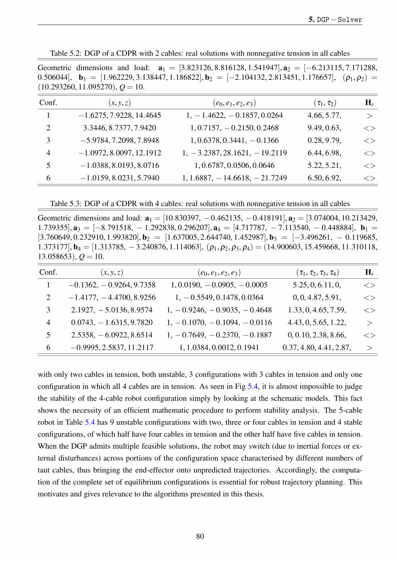
5. DGP−Solver
Table 5.2: DGP of a CDPR with 2 cables: real solutions with nonnegative tension in all cables
Geometric dimensions and load: a1 = [3.823126, 8.816128, 1.541947], a2 = [−6.213115, 7.171288,0.506044], b1 = [1.962229, 3.138447, 1.186822], b2 = [−2.104132, 2.813451, 1.176657], (ρ1, ρ2) =(10.293260, 11.095270), Q = 10.
Conf. (x, y, z) (e0, e1, e2, e3) (τ1, τ2) Hr
1 −1.6275, 7.9228, 14.4645 1, −1.4622, −0.1857, 0.0264 4.66, 5.77, >
2 3.3446, 8.7377, 7.9420 1, 0.7157, −0.2150, 0.2468 9.49, 0.63, <>
3 −5.9784, 7.2098, 7.8948 1, 0.6378, 0.3441, −0.1366 0.28, 9.79, <>
4 −1.0972, 8.0097, 12.1912 1, −3.2387, 28.1621, −19.2119 6.44, 6.98, <>
5 −1.0388, 8.0193, 8.0716 1, 0.6787, 0.0506, 0.0646 5.22, 5.21, <>
6 −1.0159, 8.0231, 5.7940 1, 1.6887, −14.6618, −21.7249 6.50, 6.92, <>
Table 5.3: DGP of a CDPR with 4 cables: real solutions with nonnegative tension in all cables
Geometric dimensions and load: a1 = [10.830397, − 0.462135, − 0.418191], a2 = [3.074004, 10.213429,1.739355], a3 = [−8.791518, − 1.292838, 0.296207], a4 = [4.717787, − 7.113540, − 0.448884], b1 =[3.760649, 0.232910, 1.993820], b2 = [1.637005, 2.644740, 1.452987], b3 = [−3.496261, − 0.119685,1.373177], b4 = [1.313785, − 3.240876, 1.114063], (ρ1, ρ2, ρ3, ρ4) = (14.900603, 15.459668, 11.310118,13.058653), Q = 10.
Conf. (x, y, z) (e0, e1, e2, e3) (τ1, τ2, τ3, τ4) Hr
1 −0.1362, −0.9264, 9.7358 1, 0.0190, −0.0905, −0.0005 5.25, 0, 6.11, 0, <>
2 −1.4177, −4.4700, 8.9256 1, −0.5549, 0.1478, 0.0364 0, 0, 4.87, 5.91, <>
3 2.1927, −5.0136, 8.9574 1, −0.9246, −0.9035, −0.4648 1.33, 0, 4.65, 7.59, <>
4 0.0743, −1.6315, 9.7820 1, −0.1070, −0.1094, −0.0116 4.43, 0, 5.65, 1.22, >
5 2.5358, −6.0922, 8.6514 1, −0.7649, −0.2370, −0.1887 0, 0.10, 2.38, 8.66, <>
6 −0.9995, 2.5837, 11.2117 1, 1.0384, 0.0012, 0.1941 0.37, 4.80, 4.41, 2.87, >
with only two cables in tension, both unstable, 3 configurations with 3 cables in tension and only oneconfiguration in which all 4 cables are in tension. As seen in Fig 5.4, it is almost impossible to judgethe stability of the 4-cable robot configuration simply by looking at the schematic models. This factshows the necessity of an efficient mathematic procedure to perform stability analysis. The 5-cablerobot in Table 5.4 has 9 unstable configurations with two, three or four cables in tension and 4 stableconfigurations, of which half have four cables in tension and the other half have five cables in tension.When the DGP admits multiple feasible solutions, the robot may switch (due to inertial forces or ex-ternal disturbances) across portions of the configuration space characterised by different numbers oftaut cables, thus bringing the end-effector onto unpredicted trajectories. Accordingly, the computa-tion of the complete set of equilibrium configurations is essential for robust trajectory planning. Thismotivates and gives relevance to the algorithms presented in this thesis.
80
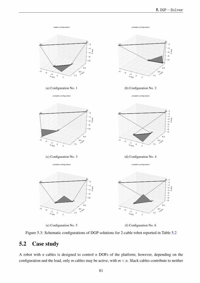
5. DGP−Solver
X axis
64
20
2
Y axis
7.5
8.0
8.5
Z a
xis
10
8
6
4
2A1
A2
B1B2
stable configuration
(a) Configuration No. 1
X axis
64
20
2
Y axis
7.5
8.0
8.5
Z a
xis
10
8
6
4
2A1
A2
B1
B2
unstable configuration
(b) Configuration No. 2
X axis
64
20
2
Y axis
7.5
8.0
8.5
Z a
xis
10
8
6
4
2A1
A2
B1
B2
unstable configuration
(c) Configuration No. 3
X axis
64
20
2
Y axis
7.5
8.0
8.5
Z a
xis
9
8
7
6
5
4
3
2
1A1A2
B1B2
unstable configuration
(d) Configuration No. 4
X axis
64
20
2
Y axis
7.5
8.0
8.5
Z a
xis
10
8
6
4
2A1
A2
B1B2
unstable configuration
(e) Configuration No. 5
X axis
64
20
2
Y axis
7.5
8.0
8.5
Z a
xis
9
8
7
6
5
4
3
2
1A1A2
B1B2
unstable configuration
(f) Configuration No. 6
Figure 5.3: Schematic configurations of DGP solutions for 2-cable robot reported in Table 5.2
5.2 Case study
A robot with n cables is designed to control n DOFs of the platform; however, depending on theconfiguration and the load, only m cables may be active, with m < n. Slack cables contribute to neither
81
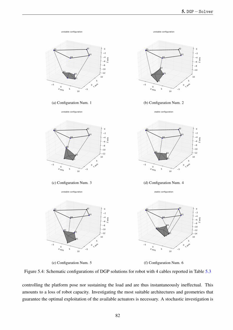
5. DGP−Solver
X axis
50
510
Y axis
5
0
5
10
Z a
xis
12
10
8
6
4
2
0
A1
A2A3
A4
B1
B2B3
B4
unstable configuration
(a) Configuration Num. 1
X axis
50
510
Y axis
5
0
5
10
Z a
xis
10
8
6
4
2
0
A1
A2A3
A4
B1
B2
B3
B4
unstable configuration
(b) Configuration Num. 2
X axis
50
510
Y axis
5
0
5
10
Z a
xis
12
10
8
6
4
2
0
A1
A2A3
A4
B1
B2
B3
B4
unstable configuration
(c) Configuration Num. 3
X axis
50
510
Y axis
5
0
5
10
Z a
xis
12
10
8
6
4
2
0
A1
A2A3
A4
B1
B2B3
B4
stable configuration
(d) Configuration Num. 4
X axis
50
510
Y axis
5
0
5
10
Z a
xis
12
10
8
6
4
2
0
A1
A2A3
A4
B1
B2B3
B4
unstable configuration
(e) Configuration Num. 5
X axis
50
510
Y axis
5
0
5
10
Z a
xis
14
12
10
8
6
4
2
0
A1
A2A3
A4
B1B2
B3
B4
stable configuration
(f) Configuration Num. 6
Figure 5.4: Schematic configurations of DGP solutions for robot with 4 cables reported in Table 5.3
controlling the platform pose nor sustaining the load and are thus instantaneously ineffectual. Thisamounts to a loss of robot capacity. Investigating the most suitable architectures and geometries thatguarantee the optimal exploitation of the available actuators is necessary. A stochastic investigation is
82
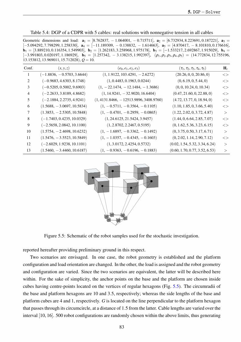
5. DGP−Solver
Table 5.4: DGP of a CDPR with 5 cables: real solutions with nonnegative tension in all cables
Geometric dimensions and load: a1 = [8.762837, − 1.064001, − 0.715711], a2 = [6.732934, 8.223691, 0.187221], a3 =[−5.094292, 7.798299, 1.258330], a4 = [−11.189309, − 0.138832, − 1.614663], a5 = [4.870417, − 8.101810, 0.176616],b1 = [3.889210, 0.116354, 1.549903], b2 = [1.262183, 3.258968, 1.975178], b3 = [−1.533217, 2.692867, 1.915029], b4 =[−3.991803, 0.020197, 1.186929], b5 = [1.257342, − 3.138215, 1.992397], (ρ1, ρ2, ρ3, ρ4, ρ5) = (14.772834, 12.755196,13.153812, 13.969011, 15.712028), Q = 10.
Conf. (x, y, z) (e0, e1, e2, e3) (τ1, τ2, τ3, τ4, τ5) Hr
1 (−1.8836, −0.5703, 3.6644) (1, 1.9122, 103.4291, −2.6272) (20.26, 0, 0, 20.86, 0) <>
2 (−0.9683, 4.6303, 8.1748) (1, 0.4483, 0.1963, 0.0244) (0, 6.19, 0, 5.44, 0) <>
3 (−0.5205, 0.5002, 9.6903) (1, −22.1474, −12.1484, −1.3686) (0, 0, 10.24, 0, 10.34) <>
4 (−2.2633, 3.8189, 4.8682) (1, 14.9241, −32.9020, 16.6404) (0.47, 21.60, 0, 22.88, 0) <>
5 (−2.1884, 2.2735, 4.9241) (1, 4131.8466, −12513.9896, 3408.9760) (4.72, 13.77, 0, 18.94, 0) <>
6 (1.5688, −3.0697, 10.5834) (1, −0.5711, −0.3564, −0.1105) (1.10, 1.85, 0, 3.66, 5.40) <>
7 (1.3853, −2.5305, 10.5848) (1, −0.4701, −0.2959, −0.0865) (1.22, 2.02, 0, 3.72, 4.87) >
8 (−1.7403, 0.4235, 10.0329) (1, 24.6125, 21.5424, 3.9457) (1.44, 0, 6.64, 2.85, 7.07) <>
9 (−2.5658, 2.0842, 10.1100) (1, 2.8702, 2.2467, 0.5195) (0, 1.62, 5.36, 3.23, 6.15) <>
10 (1.5754, −2.4698, 10.6232) (1, −1.6897, −0.3362, −0.1492) (0, 3.75, 0.50, 3.17, 6.71) >
11 (1.5476, −3.5523, 10.5849) (1, −1.0357, −0.4345, −0.1603) (0, 2.02, 1.14, 2.90, 7.12) <>
12 (−2.6029, 1.9238, 10.1101) (1, 3.0172, 2.4254, 0.5732) (0.02, 1.54, 5.32, 3.34, 6.24) >
13 (1.5460, −3.4460, 10.6187) (1, −0.9363, −0.6196, −0.1883) (0.60, 1.70, 0.77, 3.52, 6.53) >
Figure 5.5: Schematic of the robot samples used for the stochastic investigation.
reported hereafter providing preliminary ground in this respect.Two scenarios are envisaged. In one case, the robot geometry is established and the platform
configuration and load orientation are changed. In the other, the load is assigned and the robot geometryand configuration are varied. Since the two scenarios are equivalent, the latter will be described herewithin. For the sake of simplicity, the anchor points on the base and the platform are chosen insidecubes having centre-points located on the vertices of regular hexagons (Fig. 5.5). The circumradii ofthe base and platform hexagons are 10 and 3.5, respectively; whereas the side lengths of the base andplatform cubes are 4 and 1, respectively. G is located on the line perpendicular to the platform hexagonthat passes through its circumcircle, at a distance of 1.5 from the latter. Cable lengths are varied over theinterval [10, 16]. 500 robot configurations are randomly chosen within the above limits, thus generating
83
5. DGP−Solver
500 samples of 6-cable robots. For each sample, DGP−Solver computes the overall solution set, S.The latter comprises all solutions of the DGP such that {‖ si ‖≤ ρi, i = 1 . . .6}, where the equalityholds for taut cables and the inequality for slack cables. By ignoring the constraint ‖ si ‖≤ ρi for 6− k
cables, 500(6
k
)additional samples of k-cable robots with k = 2 . . .5 may be easily extracted from the
DGP−Solver computation1.Accordingly, a large sample of robots with m cables, m < n, may be derived from the same simula-
tions. For example, ifW ⊆ {1, 2, 3, 4, 5}, enforcing ‖ A6−B6 ‖≤ ρ6 provides an admissible configu-ration of the 6-cable robot with only 5 cables in tension; whereas neglecting it provides an admissibleconfiguration of the 5-cable robot with all cables in tension. In particular, among the 500 sample 6-cable CDPR geometries, 7500 robots with 2 cables, 10000 robots with 3 cables, 7500 robots with 4cables and 3000 robots with 5 cables are derived. The results of the simulation are summarised inTable 5.5. The nth column, with n = 2 . . .6, reports the results obtained for the samples suspended byn cables and, in particular, the number of samples considered (row 1), the number of feasible config-urations globally obtained (row 2) and the number of feasible configurations with m cables in tension,m≤ n (row 2+m).
The data emerging from the table appears to show that, when the number of cables increases, theprobability of finding feasible configurations with all cables in tension decreases. For the robots with2 cables, almost 90% of equilibrium configurations have both cables as active, whereas for the robotswith 3 cables, all cables are active in roughly 80% of cases. This trend continues as n increases, until,for the samples with 6 cables, almost no configurations are present with all 6 cables being active.Columns 4 through 6 show that, in most cases, the robots with 4 cables have only 3 taut cables,whereas the robots with 5 and 6 cables have only 3 or 4 cables in tension. It is worth noting that, whileequilibrium configurations with slack cables may only occur at the frontier of the geometric workspace2
for robots with 2 or 3 cables, this is not the case when n ≥ 4, where equilibrium configurations withslack cables may occur in the middle of the workspace.
Another interesting issue concerns the probability of a CDPR admitting multiple feasible configu-rations. When this occurs, the stable equilibrium pose of the platform may change under the influenceof external perturbations, which is not favourable in practice. In this context, Table 5.6 investigates thenumber of multiple solutions encountered when solving the DGP of the samples in Table 5.5. Rows2, 3 and 4 report the percentages of samples admitting 1, 2 or more feasible solutions, respectively. Itis evident that, when the number of cables increases, the probability of having a single solution of theDGP decreases. It is roughly 83% for the 3-cable robots, 53% for the 4-cable samples and a little lessthan 25% for the 5- and the 6-cable robots.
From the data reported in Tables 5.5 and 5.6, one could argue that, as long as only 3 cables areemployed, all of them may reasonably be expected to support the platform with a single stable equi-librium pose being unambiguously determined in most circumstances. When 4, 5 or 6 cables are used,
1 As explained in Section 5.1, DGP−Solver provides the DGP solutions for all possible constraint sets CW = {‖s j ‖= ρ j, τ j > 0, j ∈W}, withW ⊆ {1, 2, 3, 4, 5, 6}, m = card(W) ≤ 6 and {‖ sk ‖≤ ρk, ∀k /∈W}. By ignoring the latterrequirement, the DGP solutions for CW provide the equilibrium configurations of a robot including only m cables.
2 When a single cable is taut, the external wrench, QLe, must be aligned with it. When n = 3 and only two cables aretaut, the latter and QLe must be coplanar (Carricato [2013b]; Carricato and Merlet [2013]).
84

5. DGP−Solver
full control of the robot becomes challenging, as it is difficult to take advantage of all available cables.Controlling the platform pose in a deterministic way in this case is therefore not simple.
Table 5.5: Stochastic analysis of random samples of robot geometries with 2, 3, 4, 5 and 6 cables.
n-n CDPRs 2-2 CDPRs 3-3 CDPRs 4-4 CDPRs 5-5 CDPRs 6-6 CDPRs
No. of samples 7500 10000 7500 3000 500
No. of feasible solutions 7500 12048 12006 5912 1114
No. of feasible solutionswith 1 active cable
785(10.46%) 70(0.58%) 0 0 0
No. of feasible solutionswith 2 active cables
6715(89.53%) 2424(20.11%) 109(0.90%) 3(0.05%) 0
No. of feasible solutionswith 3 active cables
− 9554(79.29%) 6987(58.19%) 2362(39.95%) 380(34.11%)
No. of feasible solutionswith 4 active cables
− − 4910(40.89%) 2626(44.41%) 420(37.70%)
No. of feasible solutionswith 5 active cables
− − − 921(15.57%) 312(28.00%)
No. of feasible solutionswith 6 active cables
− − − − 2(0.17%)
Table 5.6: Distribution of multiple feasible configurations as emerging from stochastic analysis.
parbox[t]1.4inn-n CDPRs 2-2 CDPRs 3-3 CDPRs 4-4 CDPRs 5-5 CDPRs 6-6 CDPRs
No. of samples 7500 10000 7500 4000 500
No. of cases with 1 feasi-ble solutions
7500(100%) 8320(83.20%) 3941(52.54%) 988(24.70%) 113(22.60%)
No. of cases with 2 feasi-ble solutions
0 1299(12.99%) 2754(36.72%) 1276(31.90%) 213(42.60%)
No. of cases with morethan 2 feasible solutions
0 381(3.81%) 805(10.73%) 736(18.40%) 174(34.80%)
85

Chapter 6
Conclusions
In this dissertation, the geometric static problem of under-constrained cable-driven parallel robots (CD-PRs) supported by n cables, with n ≤ 6, was studied. The task consisted of finding the overall equi-librium configurations of a robot subject to both geometric and static constraints; namely, with n robotvariables and a static load assigned. The kinematics and statics are coupled and must be solved si-multaneously, which is a major challenge. When n constraints are imposed on the moving platform,an inverse geometric static problem is concerned, which consists of computing the overall pose of theplatform, the cable lengths and the cable tensions. The direct geometric static problem consists ofdetermining the platform posture and cable tensions when the n cable lengths are assigned. In orderto propose a sufficient solution strategy, the problem was modelled by a set of algebraic equations inChapter 3.
In Chapter 4, least-degree univariate polynomials in the ideal corresponding to particular IGPs andDGPs were found for any value of n by using an appropriate elimination procedure, thus setting anexact bound on the number of solutions admitted in the complex field. The IGP was less complexand, by introducing some ingenious strategies, was solved with the attainment of low-order univariatepolynomials. The most challenging tasks were associated with the DGP for n = 3, 4 and 5, wherethe aforementioned polynomials had degrees as high as 156, 216 and 140, respectively. Though thesepolynomials proved to be too large to be numerically useful, they provided meaningful benchmarks totest the effectiveness of an innovative variable-elimination procedure. It was proven that this proce-dure may succeed when other methods either fail or are too computationally onerous, thus providingan efficient alternative in calculating a least-degree univariate polynomial in a given ideal; a classicchallenge in robot analysis and synthesis. For the numerical computation of the solution set, a nu-merical procedure based on homotopy continuation was developed. As discussed in Chapter 4, thisis a path-tracking technique that transforms a start system of polynomial equations with known so-lutions to a target system whose solutions must be found. In general, homotopy continuation, withno information about the roots of the target system, sees the construction of a start system yieldingthe maximum possible number of solutions, equal to the Bezout number. Converting the start systemof the equation to the target one and tracking all solution paths, many such paths diverge to infinity,while only a limited number converge to finite solutions. Usually this number of paths is much largerthan the finite solutions of the target system of equations in the complex field and, as a result, tracking
86
6. Conclusions
diverging paths causes significant and non-beneficial computational burden. It has been demonstratedthat the Bezout number and corresponding number of tracked paths may be significantly smaller ifthe corresponding system of equations are multi-homogenised, yielding faster algorithm execution.On the other hand, when all nonsingular isolated roots of solutions to a general member of a familyof equations are known, ‘coefficient-parameter’ homotopy continuation may be implemented to findsolutions for any other robots of the same family in a more efficient way. Accordingly, by a suitablehomotopy, only the paths originating at the isolated roots of the start system were tracked; whereasthose corresponding to solutions going to infinity were ignored.
Another challenge addressed in this thesis was determination of the maximum number of real solu-tions admitted by the studied systems. The solutions of each problem may be complex or real, but onlythe latter have physical interest. By varying robot parameters, the number of real roots varies. Due tothe very high number of solutions attained during the direct displacement analysis of under-constrainedCDPRs, a systematic procedure to find a set of robot parameters with the maximum number of realsolutions was necessary. Accordingly, a procedure borrowed from the Dietmaier was introduced inSection 2.3 to find sets of CDPR parameters for which the DGP provided the highest number of realconfigurations. Dietmaier’s algorithm, like the homotopy method, is a continuation procedure in whicha start system is defined for a given set of robot parameters and an iterative procedure is established tochange the system parameters and conveniently vary the solution set. In contrast with parameter ho-motopy, however, the target parameters are unknown a priori. The tracked path is adaptively modifiedin such a way that, at each iteration, the imaginary parts of some complex solutions are decreased andeventually as many complex roots as possible are transformed into real roots. By applying this tech-nique on the DGP of CDPRs with 3, 4 and 5 cables, the maximum number of real solutions obtainedfor each case was 54, 98 and 74, respectively.
By taking advantage of the homotopy continuation procedure, a program DGP−Solver was com-posed, which is freely available. The code receives the robot geometry, cable lengths and external loadas inputs and computes, under the assumption that cables are inextensible and massless, all possibleequilibrium configurations of the robot that are compatible with the given constraints. Distinctive fea-tures of the code are that it finds all solutions of the problem, including those with slack cables, andassesses the feasibility of each configuration with an integrated stability analysis.
It was shown that the DGP may admit multiple equilibrium configurations, characterised by dif-ferent numbers of taut cables. Since slack cables contribute to neither controlling the platform posenor sustaining the load, they represent a loss of capacity of the robot, which is instantaneously unableto control some of the end-effector degrees of freedom. A preliminary investigation was performed tofind the most suitable architectures that guarantee an optimal exploitation of the available actuators.The probability of a CDPR admitting multiple stable equilibrium configurations (which is a criticalsituation for reliable robot control) was also considered. From the data reported in Chapter 5, onecould argue that, as long as only 3 cables are employed, all of them may be reasonably expected tosupport the platform, with a single stable equilibrium pose being unambiguously determined in mostcircumstances.
87

Appendix A
In this section, numerical examples of geometric parameters admitting the maximum number of realsolutions for robots with 3, 4 and 5 cables are provided. These examples are the results of the Dietmaierprocedure outlined in Section 4.3 .
88

Table 1: All real solutions of DGP of a 3-3 CDPR with maximum number of 54 real solutionsGeometric dimensions and load: a1 = [0, 0, 0], a2 = [0.897440, 0, − 0.726510], a3 = [0.656710, 0.746360, − 0.590910],b1 = [1.556650, 0, 0], b2 = [0.696950, 0.784290, 0], b3 = [−0.464410, − 1.389800, − 1.199480], (ρ1, ρ2, ρ3) = (1, 1.080500,2.602500), Q = 10.
Conf. (x, y, z) (e1, e2, e3) (τ1, τ2, τ3)
1 0.0634, 0.1736, −0.5293 −0.5534, −0.9854, −0.8871 10.54, −1.21, −2.76
2 0.9948, −0.0455, −2.1045 1.0390, −0.9800, 1.2955 −9.48, −8.99, 2.33
3 0.5102, −0.1635, −0.5159 −2.1568, −2.2788, −1.9020 4.74, 6.43, 3.13
4 1.4323, 1.0452, −1.6514 2.4261, −2.8663, 3.6663 −50.28, −5.73, 49.47
5 0.2508, −0.0479, −0.6094 −0.2969, −1.0008, −0.0929 6.22, 7.93, 7.49
6 0.6483, 1.1466, −1.8930 −0.8594, −0.3795, −1.1743 −19.92, 14.07, −12.01
7 0.8516, −0.0142, −0.6959 0.1903, −1.3668, −0.5069 0.75, 11.32, 3.08
8 1.1117, −0.1800, −0.4811 6.0423, 13.3840, 4.2951 8.82, 15.20, 19.36
9 0.3744, −0.0308, −0.5111 −1.0816, −1.3568, −1.2971 5.90, 4.25, 0.53
10 0.6098, 0.0192, −1.3549 −0.1640, −0.8795, 0.2065 4.13, −17.24, −16.32
11 0.9362, −0.0509, −1.6747 −0.5647, −3.6481, −0.2073 0.22, −16.05, −13.65
12 0.6129, 0.6724, 0.9651 41.9368, −0.5618, −44.3965 −6.59, 0.34, 7.95
13 0.8858, −0.4903, −0.4509 3.2461, 4.1824, 2.4811 7.60, 12.71, 10.87
14 0.5614, 0.9292, 0.2029 −2.1638, 2.1129, 0.0571 4.71, 6.89, 10.66
15 1.2810, 0.0257, −0.5133 1.1515, 6.1838, 2.4650 5.59, 22.92, 21.84
16 0.8983, −0.0179, −0.6935 0.1435, −1.3928, −0.8091 0.11, 10.46, 0.92
17 0.9443, 0.0077, −2.1090 0.9186, −1.1658, 0.9016 −6.21, −8.26, −1.22
18 0.5369, 0.7693, −1.4696 0.0993, −0.6693, −0.3427 2.19, −5.25, −12.46
19 2.4401, 0.6365, −0.0380 −0.1171, 2.9441, −5.6330 −33.47, 26.48, 8.84
20 0.6796, 0.5035, 0.4579 −1.9056, 7.1397, −7.5311 13.67, −11.31, 6.92
21 0.4697, 0.4552, 0.0534 −0.7309, 2.0689, −0.7835 −3.12, −0.96, 8.20
22 0.5715, 0.7385, 0.1670 −3.1734, 3.2184, −0.9303 1.89, 2.70, 8.87
23 0.8954, 0.1520, 1.1534 0.0756, 0.9074, −1.2974 −1.40, 7.54, 4.01
24 0.8223, 0.6116, −1.6669 −0.1435, −2.9073, −1.4004 1.17, −12.89, −16.32
25 0.6759, 0.4964, 1.0546 −7.6257, −3.8442, 14.9347 −2.93, 6.20, 5.79
26 0.7150, −0.3392, 0.2513 −0.0682, −4.2850, 3.2341 39.94, −33.98, −3.74
27 −0.6475, 0.0685, 0.2574 1.2351, 0.4542, −0.5850 −26.32, −16.34, −1.68
28 0.8120, 0.3450, 1.0225 3.6139, 1.2486, −3.7415 −2.95, 4.97, 4.64
29 0.0000, 0.0003, −0.5566 −2.3817, −0.9993, −2.3831 10.00, −0.01, −0.00
30 0.4932, 0.0208, −0.6134 −0.5848, −1.4390, −0.2065 4.63, 9.31, 10.44
31 1.0589, −0.4306, −0.4556 1.8378, 3.0461, 2.0388 5.60, 14.99, 9.91
32 1.5486, 0.4002, −1.7581 −1.0092, −1.1007, −1.8713 −23.04, 20.76, −4.92
33 1.6482, 1.5973, −0.6567 0.3694, −0.9632, −2.6851 59.39, 2.61, −66.98
34 0.6244, 0.3345, 0.9358 0.4628, 3.4054, −5.7540 −11.53, 15.27, 5.13
35 0.2263, −0.0531, −0.6094 −0.2882, −0.9769, −0.0852 6.43, 7.76, 7.32
36 0.7741, 0.8653, −1.9269 −0.8376, −0.8822, −1.0477 −7.99, 1.73, −9.57
89
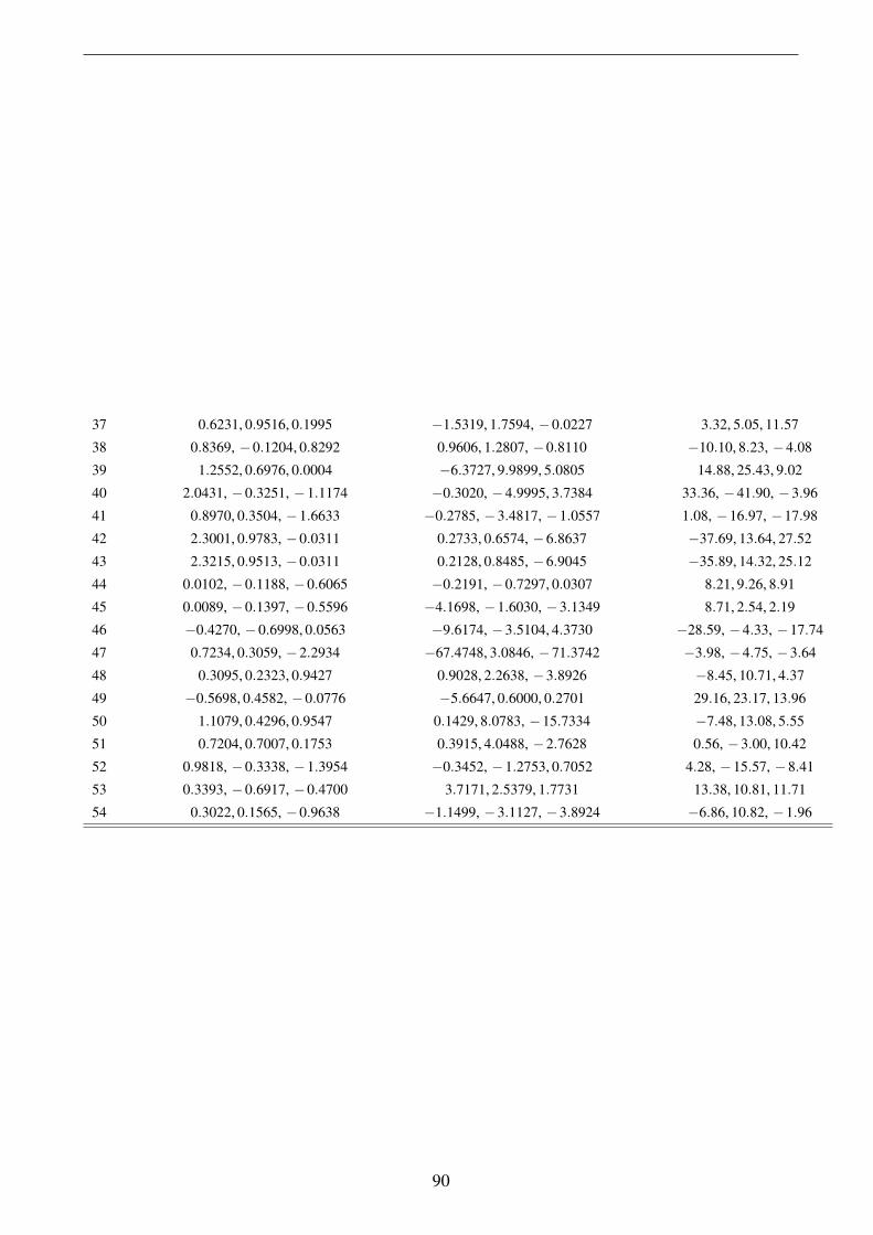
37 0.6231, 0.9516, 0.1995 −1.5319, 1.7594, −0.0227 3.32, 5.05, 11.57
38 0.8369, −0.1204, 0.8292 0.9606, 1.2807, −0.8110 −10.10, 8.23, −4.08
39 1.2552, 0.6976, 0.0004 −6.3727, 9.9899, 5.0805 14.88, 25.43, 9.02
40 2.0431, −0.3251, −1.1174 −0.3020, −4.9995, 3.7384 33.36, −41.90, −3.96
41 0.8970, 0.3504, −1.6633 −0.2785, −3.4817, −1.0557 1.08, −16.97, −17.98
42 2.3001, 0.9783, −0.0311 0.2733, 0.6574, −6.8637 −37.69, 13.64, 27.52
43 2.3215, 0.9513, −0.0311 0.2128, 0.8485, −6.9045 −35.89, 14.32, 25.12
44 0.0102, −0.1188, −0.6065 −0.2191, −0.7297, 0.0307 8.21, 9.26, 8.91
45 0.0089, −0.1397, −0.5596 −4.1698, −1.6030, −3.1349 8.71, 2.54, 2.19
46 −0.4270, −0.6998, 0.0563 −9.6174, −3.5104, 4.3730 −28.59, −4.33, −17.74
47 0.7234, 0.3059, −2.2934 −67.4748, 3.0846, −71.3742 −3.98, −4.75, −3.64
48 0.3095, 0.2323, 0.9427 0.9028, 2.2638, −3.8926 −8.45, 10.71, 4.37
49 −0.5698, 0.4582, −0.0776 −5.6647, 0.6000, 0.2701 29.16, 23.17, 13.96
50 1.1079, 0.4296, 0.9547 0.1429, 8.0783, −15.7334 −7.48, 13.08, 5.55
51 0.7204, 0.7007, 0.1753 0.3915, 4.0488, −2.7628 0.56, −3.00, 10.42
52 0.9818, −0.3338, −1.3954 −0.3452, −1.2753, 0.7052 4.28, −15.57, −8.41
53 0.3393, −0.6917, −0.4700 3.7171, 2.5379, 1.7731 13.38, 10.81, 11.71
54 0.3022, 0.1565, −0.9638 −1.1499, −3.1127, −3.8924 −6.86, 10.82, −1.96
90
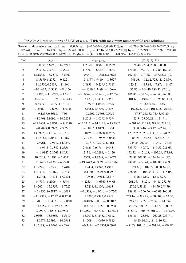
Table 2: All real solutions of DGP of a 4-4 CDPR with maximum number of 98 real solutionsGeometric dimensions and load: a1 = [0, 0, 0], a2 = [−0.760549, 0, 0.909316], a3 = [−0.716460, 0.680475, 0.079703], a4 =[0.025744, 0.704210, 0.873897], b1 = [16.548180, 0, 0], b2 = [17.163583, 0.777200, 0], b3 = [16.222490, 0.751536, 0.768740],b4 = [17.386036, 0.095675, 0.817269], (ρ1, ρ2, ρ3, ρ4) = (1, −1.014940, −1.121710, 1.138240), Q = 10.
Conf. (x, y, z) (e1, e2, e3) (τ1, τ2, τ3, τ4)
1 −3.0636, 3.6998, −16.5218 1.2350, −0.9881, 0.8529 28.40, 27.84, 28.89, 28.20,
2 15.5132, 2.5903, −4.9524 1.7397, −8.0431, 7.1683 170.86, −97.16, −112.86, 162.36,
3 13.1838, −8.2574, −3.5469 −0.0401, −1.3812, 2.6625 102.30, −307.78, −337.65, 34.17,
4 11.5670, 6.2772, −9.4221 −3.1177, 1.9410, −8.3627 −741.38, −12.62, 723.44, 128.59,
5 −11.6506, 0.2819, −11.4601 6.8831, −0.2595, 2.9118 −123.21, −115.84, 147.87, −14.07,
6 −10.4613, 11.3382, −8.0156 −4.1399, 1.3489, −1.6696 36.85, −104.40, 186.37, 87.31,
7 10.9196, −11.7787, −1.5815 −30.6642, −70.4630, −12.3521 106.85, −32.59, −268.48, 263.88,
8 −8.6254, −13.1375, −4.6443 3.4338, 1.7411, 1.2351 1101.60, −190.69, −1096.86, 1.21,
9 0.4579, −0.2077, 17.2784 −0.9776, 1.0344, 0.9627 10.16, 0.67, 5.46, −7.69,
10 −7.5948, −12.6090, −6.9715 3.1084, 1.4708, 1.4897 −1025.22, 19.34, 1014.02, 176.33,
11 −9.1237, 0.8618, 14.7504 −0.2707, 0.5708, 0.0957 −167.87, 262.52, 74.43, 93.20,
12 −1.2968, 2.9696, −16.5224 1.2218, −1.0292, 0.9594 23.34, 23.20, 21.14, 21.91,
13 −11.0831, −7.8604, −9.5570 −43.5416, −14.2111, −15.2502 −301.63, 126.92, 287.66, 231.30,
14 −0.7078, 0.3997, 17.3022 −0.8216, 1.0171, 0.7931 3.00, 3.46, −3.42, −2.46,
15 13.3972, −1.1048, −9.7319 0.0425, −2.7658, 0.3565 12.82, 287.02, −114.72, −241.29,
16 −11.6161, 1.7051, −11.4871 19.1728, −0.9528, 8.0644 −88.24, −80.58, 139.66, 20.18,
17 −9.9961, −2.9112, 14.0549 −2.3816, 0.2279, 1.3161 −245.54, 207.84, −70.40, −24.45,
18 −16.9518, 0.3842, 1.2556 2.4621, 0.0476, −0.0431 333.77, −49.79, −115.57, 281.65,
19 −16.9147, 2.8563, 1.8056 1.2138, −0.0294, −0.1204 172.32, −121.63, −107.24, 173.98,
20 10.0205, 13.1293, −5.4691 1.3368, −3.1248, −0.6672 71.81, 203.92, −134.34, −1.42,
21 13.5463, 8.6135, −4.8598 −19.7447, 49.3021, −38.2869 281.05, −39.41, −109.85, 252.90,
22 11.2216, −9.9730, −6.4402 1.2434, 1.4742, 3.4988 −191.86, −102.77, 28.30, 69.28,
23 11.8391, −8.3162, −7.7833 −0.4730, −2.4900, 0.7901 226.98, −1106.38, 41.91, 1115.05,
24 −1.2041, −0.4941, 17.2804 −0.9000, 0.9551, 0.8716 5.26, 12.60, −1.54, 6.27,
25 14.7591, 6.2906, −4.8544 4.2253, −14.6369, 8.9408 261.35, −81.21, −64.15, 272.76,
26 3.4207, −15.5757, −1.7527 3.7214, 4.6109, 1.9663 276.39, 58.21, −434.59, 298.79,
27 −5.4436, 16.2817, −1.3017 −0.0318, −0.0510, −0.7501 189.51, −256.56, −67.01, 163.51,
28 −11.4917, −12.2734, 0.1200 1.0395, 0.4993, 0.4527 263.16, −398.88, −508.04, −63.00,
29 −1.7881, −11.4731, −12.0581 −0.4036, −0.9176, 0.3017 29.77, 103.85, −75.37, −147.94,
30 −1.8657, 11.1139, 13.3556 −0.7322, 1.1125, −0.0938 −361.45, 160.02, −134.48, −209.23,
31 3.2997, 10.6518, 13.3938 14.2253, −9.4774, −13.8594 −575.10, −308.78, 601.30, −1117.08,
32 7.9368, −13.9365, −1.5610 18.0074, 31.2452, 7.0112 136.81, −23.94, −267.28, 233.74,
33 −1.2579, 2.3595, −16.5964 1.1209, −1.0636, 0.9813 16.20, 16.01, 18.16, 16.72,
34 11.6118, −7.0364, −9.2964 −0.3474, −2.3354, 0.5990 −54.28, 1011.71, −204.69, −989.87,
91
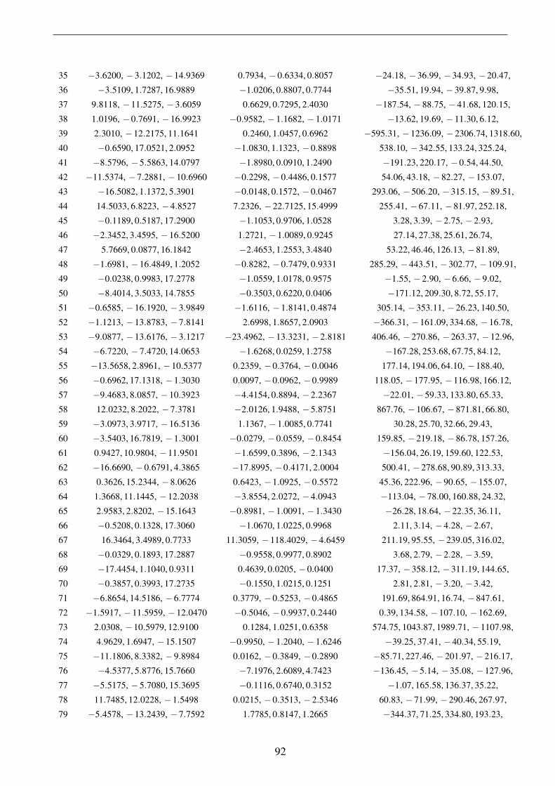
35 −3.6200, −3.1202, −14.9369 0.7934, −0.6334, 0.8057 −24.18, −36.99, −34.93, −20.47,
36 −3.5109, 1.7287, 16.9889 −1.0206, 0.8807, 0.7744 −35.51, 19.94, −39.87, 9.98,
37 9.8118, −11.5275, −3.6059 0.6629, 0.7295, 2.4030 −187.54, −88.75, −41.68, 120.15,
38 1.0196, −0.7691, −16.9923 −0.9582, −1.1682, −1.0171 −13.62, 19.69, −11.30, 6.12,
39 2.3010, −12.2175, 11.1641 0.2460, 1.0457, 0.6962 −595.31, −1236.09, −2306.74, 1318.60,
40 −0.6590, 17.0521, 2.0952 −1.0830, 1.1323, −0.8898 538.10, −342.55, 133.24, 325.24,
41 −8.5796, −5.5863, 14.0797 −1.8980, 0.0910, 1.2490 −191.23, 220.17, −0.54, 44.50,
42 −11.5374, −7.2881, −10.6960 −0.2298, −0.4486, 0.1577 54.06, 43.18, −82.27, −153.07,
43 −16.5082, 1.1372, 5.3901 −0.0148, 0.1572, −0.0467 293.06, −506.20, −315.15, −89.51,
44 14.5033, 6.8223, −4.8527 7.2326, −22.7125, 15.4999 255.41, −67.11, −81.97, 252.18,
45 −0.1189, 0.5187, 17.2900 −1.1053, 0.9706, 1.0528 3.28, 3.39, −2.75, −2.93,
46 −2.3452, 3.4595, −16.5200 1.2721, −1.0089, 0.9245 27.14, 27.38, 25.61, 26.74,
47 5.7669, 0.0877, 16.1842 −2.4653, 1.2553, 3.4840 53.22, 46.46, 126.13, −81.89,
48 −1.6981, −16.4849, 1.2052 −0.8282, −0.7479, 0.9331 285.29, −443.51, −302.77, −109.91,
49 −0.0238, 0.9983, 17.2778 −1.0559, 1.0178, 0.9575 −1.55, −2.90, −6.66, −9.02,
50 −8.4014, 3.5033, 14.7855 −0.3503, 0.6220, 0.0406 −171.12, 209.30, 8.72, 55.17,
51 −0.6585, −16.1920, −3.9849 −1.6116, −1.8141, 0.4874 305.14, −353.11, −26.23, 140.50,
52 −1.1213, −13.8783, −7.8141 2.6998, 1.8657, 2.0903 −366.31, −161.09, 334.68, −16.78,
53 −9.0877, −13.6176, −3.1217 −23.4962, −13.3231, −2.8181 406.46, −270.86, −263.37, −12.96,
54 −6.7220, −7.4720, 14.0653 −1.6268, 0.0259, 1.2758 −167.28, 253.68, 67.75, 84.12,
55 −13.5658, 2.8961, −10.5377 0.2359, −0.3764, −0.0046 177.14, 194.06, 64.10, −188.40,
56 −0.6962, 17.1318, −1.3030 0.0097, −0.0962, −0.9989 118.05, −177.95, −116.98, 166.12,
57 −9.4683, 8.0857, −10.3923 −4.4154, 0.8894, −2.2367 −22.01, −59.33, 133.80, 65.33,
58 12.0232, 8.2022, −7.3781 −2.0126, 1.9488, −5.8751 867.76, −106.67, −871.81, 66.80,
59 −3.0973, 3.9717, −16.5136 1.1367, −1.0085, 0.7741 30.28, 25.70, 32.66, 29.43,
60 −3.5403, 16.7819, −1.3001 −0.0279, −0.0559, −0.8454 159.85, −219.18, −86.78, 157.26,
61 0.9427, 10.9804, −11.9501 −1.6599, 0.3896, −2.1343 −156.04, 26.19, 159.60, 122.53,
62 −16.6690, −0.6791, 4.3865 −17.8995, −0.4171, 2.0004 500.41, −278.68, 90.89, 313.33,
63 0.3626, 15.2344, −8.0626 0.6423, −1.0925, −0.5572 45.36, 222.96, −90.65, −155.07,
64 1.3668, 11.1445, −12.2038 −3.8554, 2.0272, −4.0943 −113.04, −78.00, 160.88, 24.32,
65 2.9583, 2.8202, −15.1643 −0.8981, −1.0091, −1.3430 −26.28, 18.64, −22.35, 36.11,
66 −0.5208, 0.1328, 17.3060 −1.0670, 1.0225, 0.9968 2.11, 3.14, −4.28, −2.67,
67 16.3464, 3.4989, 0.7733 11.3059, −118.4029, −4.6459 211.19, 95.55, −239.05, 316.02,
68 −0.0329, 0.1893, 17.2887 −0.9558, 0.9977, 0.8902 3.68, 2.79, −2.28, −3.59,
69 −17.4454, 1.1040, 0.9311 0.4639, 0.0205, −0.0400 17.37, −358.12, −311.19, 144.65,
70 −0.3857, 0.3993, 17.2735 −0.1550, 1.0215, 0.1251 2.81, 2.81, −3.20, −3.42,
71 −6.8654, 14.5186, −6.7774 0.3779, −0.5253, −0.4865 191.69, 864.91, 16.74, −847.61,
72 −1.5917, −11.5959, −12.0470 −0.5046, −0.9937, 0.2440 0.39, 134.58, −107.10, −162.69,
73 2.0308, −10.5979, 12.9100 0.1284, 1.0251, 0.6358 574.75, 1043.87, 1989.71, −1107.98,
74 4.9629, 1.6947, −15.1507 −0.9950, −1.2040, −1.6246 −39.25, 37.41, −40.34, 55.19,
75 −11.1806, 8.3382, −9.8984 0.0162, −0.3849, −0.2890 −85.71, 227.46, −201.97, −216.17,
76 −4.5377, 5.8776, 15.7660 −7.1976, 2.6089, 4.7423 −136.45, −5.14, −35.08, −127.96,
77 −5.5175, −5.7080, 15.3695 −0.1116, 0.6740, 0.3152 −1.07, 165.58, 136.37, 35.22,
78 11.7485, 12.0228, −1.5498 0.0215, −0.3513, −2.5346 60.83, −71.99, −290.46, 267.97,
79 −5.4578, −13.2439, −7.7592 1.7785, 0.8147, 1.2665 −344.37, 71.25, 334.80, 193.23,
92
80 −3.7312, 15.5777, −6.8992 0.3902, −0.6362, −0.6047 271.50, 624.55, 112.19, −615.78,
81 3.5662, 2.6486, −15.1679 −0.9527, −1.0377, −1.4724 −30.44, 24.23, −25.60, 41.73,
82 −0.2476, 11.1074, −12.2150 −3.0624, 1.3031, −3.0921 −92.70, −51.69, 144.13, 45.06,
83 −8.4154, 14.8584, −3.7961 0.3745, −0.3752, −0.5197 2.79, −930.91, −192.59, 948.96,
84 −0.4145, 17.2918, −2.5308 0.3939, −0.5353, −0.9287 −179.78, −529.68, −436.36, 708.58,
85 2.9404, 16.8826, −1.2948 0.0736, −0.1894, −1.2342 74.96, −146.05, −162.90, 197.13,
86 −0.3618, 0.4121, 17.3248 −5.0689, 0.9144, 4.9177 2.75, 2.71, −3.67, −3.07,
87 12.6637, 1.7361, −9.6306 77.1195, −31.2701, 238.2116 −314.35, −4.98, 276.00, 116.56,
88 0.1148, 16.5864, −2.7131 −0.5383, 0.3499, −1.1451 374.87, −312.55, −140.79, 30.53,
89 3.3588, 13.5767, 10.4255 3.6731, −2.7332, −3.5815 788.87, 325.61, −800.67, 1419.29,
90 0.8043, −13.7855, −8.1404 1.7219, 1.1359, 1.8345 −224.66, −56.06, 157.58, 71.34,
91 −10.1361, −10.2561, −7.6349 −0.1779, −0.3927, 0.3236 103.97, −16.28, −79.78, −165.79,
92 4.9946, 0.4885, 16.3671 −0.3346, 1.4333, 0.4389 −18.06, −34.52, 74.45, −110.36,
93 −13.0870, −1.2559, −11.1548 −0.0203, −0.3928, 0.0379 56.39, 79.86, −55.87, −144.93,
94 11.7283, 10.0478, −5.7690 0.6982, −2.7080, −1.0165 110.37, 181.38, −74.80, −18.22,
95 −0.0845, −11.3657, −12.0416 −0.2943, −0.9356, 0.4088 59.71, 101.52, −45.58, −146.25,
96 −11.6845, 12.8484, 0.8473 1.0531, −0.4355, −0.4450 347.58, −238.65, 27.03, 448.67,
97 −5.0174, 14.5255, −7.8659 0.5991, −0.7684, −0.4124 −36.81, 309.20, −174.84, −287.03,
98 15.6052, −3.8242, 2.4675 −0.4272, 0.4396, 6.4481 −107.93, −247.56, −371.75, 241.56,
93

Table 3: All real solutions of DGP of a 5-5 CDPR with maximum number of 74 real solutionsGeometric dimensions and load: a1 = [0, 0, 0], a2 = [1.444170, 0, 1.203330], a3 = [0.302415, 1.262060, 0.555330],a4 = [−0.711127, 0.808726, 0.810451], a5 = [0.749568, 0.761578, − 0.469085], b1 = [2.161690, 0, 0], b2 = [−0.125711, 0,1.326150], b3 = [−0.412791, 0.021143, 0.449869], b4 = [−0.162650, − 0.468249, − 0.399945], b5 = [1.596530, 1.314460,0.962240], (ρ1, ρ2, ρ3, ρ4) = (2.464490, 1.995860, 1.206220, 1.423950, 2.430200), Q = 10.
Conf. (x, y, z) (e1, e2, e3) (τ1, τ2, τ3, τ4)
1 −0.2837, −0.1765, 0.2861 −0.9878, −0.6538, −1.0446 11.74, 0.23, −1.94, −0.99, −2.82,
2 0.5312, 0.6906, −0.7303 −0.4333, 0.9140, −0.4121 2.86, 1.88, 17.78, 3.08, −33.92,
3 0.6764, 2.1323, 0.4556 0.1229, 1.4532, −0.3371 −135.72, −60.35, −172.56, 138.78, 189.75,
4 1.2297, 1.1158, 0.6440 −0.6782, 0.4388, −0.5549 27.02, −6.23, 48.62, −46.72, −21.12,
5 0.1548, −0.0888, 0.3115 −1.3644, −1.1945, −1.2275 10.37, 2.35, 4.15, −1.06, 3.29,
6 1.0020, 1.4049, 0.3247 −0.0524, 1.0933, 0.0764 −30.88, −15.22, −18.11, 21.28, 37.16,
7 0.1363, 0.9933, −0.9479 −0.2815, 0.9396, −0.5967 −9.63, −1.45, −25.77, 4.17, 22.46,
8 0.4281, 0.4239, −0.7045 −0.6045, 0.8501, −0.4034 16.06, 3.99, 102.86, −12.02, −118.32,
9 −0.3582, 2.1809, 0.5294 0.3037, 0.2975, −0.1669 −6.97, −16.70, 16.56, 1.98, 7.97,
10 −0.9130, 1.3560, 0.0753 83.0105, −24.9753, 80.8086 2.53, 15.28, −15.22, −6.10, 5.03,
11 −0.4607, 0.0108, 0.6416 0.5670, 4.1847, 1.1578 −82.57, 3.09, 100.70, −89.99, 63.90,
12 −1.3491, 0.9141, 0.1015 −0.9261, 0.5187, −1.8319 18.17, 5.35, 0.08, −16.88, −12.61,
13 0.5107, 0.9502, 1.1408 −0.2853, 0.4373, 0.4091 0.65, 2.09, 10.29, −1.70, −1.52,
14 −0.4694, 0.6436, 1.7056 −9.8403, 3.5712, −1.2696 1.73, 0.47, 2.31, 7.55, 0.48,
15 0.2243, 1.2378, −0.8704 −0.1238, 1.1975, −0.7995 26.07, 6.64, 64.42, −28.30, −77.52,
16 −0.1060, 1.0669, 0.0947 1.7150, −0.3236, 0.7042 7.49, 7.28, −3.92, −5.09, 5.45,
17 −0.1064, 0.1791, 1.0325 0.2008, 53.0584, −8.5358 9.20, −6.32, −1.54, 3.99, −2.06,
18 0.1132, 0.8172, 1.6214 4.1771, −0.3353, −0.6053 5.12, 4.17, 7.05, 5.87, 0.81,
19 0.3336, 0.7842, −0.4449 2.1191, 4.0645, −5.3532 −14.88, 11.74, −9.74, 0.64, −2.86,
20 −0.6706, −0.1342, 0.0699 −0.5845, 1.6081, 0.0576 140.84, −157.06, −178.83, 53.97, 100.65,
21 −0.8354, 1.8229, 1.4399 −0.2594, 2.1498, −0.4546 −4.65, −12.19, 5.94, 4.79, 9.83,
22 0.3662, 0.4199, −0.3881 1.0575, 0.7139, −1.4214 −17.64, 2.08, 13.06, 9.12, −11.98,
23 0.1825, 0.7634, 0.1265 1.1952, −0.0899, 0.0737 0.17, 0.26, −5.00, −6.20, 3.90,
24 −0.3065, 1.4008, 1.3108 0.6942, 2.2769, −4.5700 1.13, −3.68, 10.74, 2.08, 0.46,
25 −1.1314, 1.2503, 0.0753 −3.9748, 1.3324, −4.7641 −8.15, 39.49, −32.44, −9.72, 19.65,
26 −0.4868, 1.9962, 0.5210 0.4409, 0.2077, −0.1097 −15.89, −30.82, 23.22, 14.70, 14.02,
27 −0.0282, 0.5763, −0.1349 12.5513, 10.6915, 15.9334 1.01, 2.85, 14.62, −8.02, 16.18,
28 −0.5173, 1.0320, −0.1333 0.0762, 0.0876, 0.2274 −7.40, −3.38, −2.47, −4.75, 6.80,
29 0.6686, 0.2969, −0.4893 −0.9115, 0.6119, −0.4893 3.24, 5.97, −41.09, −15.81, 43.46,
30 0.1711, 0.9219, 0.0821 2.3583, −0.5316, 1.0148 1.93, 2.36, −6.87, −3.16, 4.28,
31 0.5643, 0.3875, −0.0311 1.1899, 0.3178, −0.8087 11.93, 2.32, −18.47, −23.71, 16.29,
32 −0.0973, 1.6540, 1.4568 −0.9555, 0.5756, −1.7557 6.16, −5.31, 15.58, −6.54, −2.88,
94
33 0.3553, 0.6625, −0.4498 1.6934, 2.2968, −3.4782 −10.73, 6.76, −3.29, −0.59, −4.13,
34 0.9388, 1.0269, 0.7520 1.9527, 5.9393, 0.7878 0.31, −9.18, −7.10, 7.29, 4.08,
35 0.8958, 1.5893, −0.2146 −0.0721, 1.0494, −0.3239 −32.77, −21.12, 24.89, −51.95, 71.70,
36 −0.0833, −0.1848, −0.3040 −0.9629, 1.0579, −0.2260 −41.55, −8.17, 6.11, 22.41, 12.08,
37 −0.7052, 1.5521, 1.2600 −0.2759, 1.0069, −2.2936 −3.92, −8.55, 12.72, 4.56, 5.97,
38 −1.0635, 1.2974, 0.0753 −6.4385, 2.0797, −7.1895 −1.10, 25.15, −22.27, −7.74, 10.29,
39 0.3027, 0.6760, 0.3765 −0.8220, −2.6709, 2.9390 29.39, −19.91, 27.06, −13.34, −10.95,
40 1.2054, 1.0751, 0.6343 −0.9432, 0.4714, −0.7765 43.29, −11.86, 90.21, −80.86, −40.78,
41 0.4418, 0.1927, 0.6460 −4.6140, −8.4841, −3.7763 6.59, −10.30, −14.74, 7.30, −8.84,
42 0.5834, 0.2172, −0.4841 −0.9146, 0.7383, −0.4486 −11.60, 10.30, −121.68, 4.28, 114.91,
43 −0.2089, 0.0338, 0.7458 2.7490, 10.0872, 3.3235 34.08, −10.69, −35.02, 33.31, −23.92,
44 0.0739, 1.1328, −0.9382 −0.1995, 1.0771, −0.7477 −19.16, −0.48, −54.96, 17.21, 47.24,
45 0.0665, 0.4217, 0.0153 3.5456, 4.9828, 4.6809 −11.19, −4.01, −17.20, −9.17, −9.66,
46 0.6214, 2.1929, 0.3699 0.0734, 1.2226, −0.3357 113.43, 22.03, 164.32, −125.41, −146.08,
47 0.0828, 0.5548, 1.6098 9.3285, −1.3700, −0.9277 12.03, 14.35, 4.69, 8.41, 1.44,
48 0.6561, 1.1819, −0.6655 −0.1956, 1.0172, −0.4598 25.76, 15.92, 21.10, 20.11, −87.87,
49 1.0524, 1.4965, 0.3719 −0.1824, 0.8072, −0.0598 162.26, 30.54, 168.11, −167.41, −172.36,
50 −0.5641, 1.6225, 0.3104 0.5994, 0.0851, 0.0355 19.62, 30.43, −16.93, −30.07, −10.21,
51 1.0278, 1.4705, 0.3274 −0.1251, 0.9397, −0.0072 −98.19, −33.12, −84.40, 89.32, 111.36,
52 0.4918, 2.2898, 0.3568 0.0413, 0.9774, −0.3180 28.91, −5.45, 53.02, −37.75, −32.60,
53 0.4134, 0.1282, −0.5038 −0.8628, 0.8880, −0.3873 −29.84, −7.92, −143.35, 43.19, 128.44,
54 −0.2825, 0.3675, −0.5258 0.4871, 0.5334, −1.1867 −7.76, 0.91, 2.67, −4.82, 0.67,
55 0.3368, 0.1393, 1.2652 37.5553, −5.3037, −5.5255 −20.87, −31.39, 2.14, −5.99, 0.30,
56 −0.1278, 1.1309, −0.9476 −0.1984, 1.1423, −0.8971 −5.36, 1.32, −19.30, 2.49, 10.96,
57 0.9441, 0.6527, 0.2264 −3.3534, 1.3891, −1.8684 4.42, −6.83, −3.60, 3.42, −3.75,
58 −0.0023, 0.0150, 0.6541 −0.1923, −0.1528, −0.2376 10.83, −1.39, 8.46, −11.36, −1.99,
59 −0.8793, −0.0161, 0.1400 −0.4370, 1.4731, 0.2285 −1.67, −25.10, 1.40, −5.47, 19.74,
60 −1.3614, 1.3325, 0.2694 −1.6298, 1.3744, −2.3369 29.45, 40.63, −23.49, −32.05, −17.35,
61 1.0086, 0.4496, −0.0239 −1.3156, 0.7400, −0.7150 103.08, −45.09, 186.07, −103.38, −163.28,
62 0.9379, 1.2051, 0.3295 0.1487, 1.4494, 0.3033 −12.68, −8.10, 0.90, 0.18, 16.09,
63 −0.5244, −0.1694, −0.0583 −0.6830, 1.4965, −0.0419 −213.43, 152.49, 282.18, −67.13, −122.82,
64 −0.7410, 0.5791, −0.1580 −0.1644, 0.4463, 0.4641 −8.02, −4.12, −0.78, −4.74, 5.87,
65 1.1280, 0.9932, 0.4236 −1.5807, 0.5910, −1.2229 −36.84, 14.13, −97.02, 75.50, 49.11,
66 −0.5693, 0.6741, −0.1965 −9.3397, −4.2033, −12.1619 1.05, 1.18, 1.17, −8.09, 3.26,
67 −0.3987, 0.7036, −0.0598 −0.0816, 0.0974, 0.3804 −46.55, 0.93, −33.89, 16.34, 29.91,
68 0.1908, 0.7721, −0.1539 35.9920, 22.1885, 43.1066 0.31, −0.08, 2.01, −5.41, 6.39,
69 −0.1649, 0.5597, 0.1779 −0.1225, −0.0087, 0.3862 66.76, −11.03, 55.50, −40.37, −38.80,
70 −0.8399, 1.3674, 0.0753 12.4335, −3.6207, 11.3678 3.07, 12.97, −13.50, −5.73, 4.12,
71 −1.3369, 1.4526, 0.9523 −1.6895, 1.9967, −1.7759 −36.66, −36.43, 18.11, 29.54, 28.35,
72 −0.0556, 1.0020, 0.1161 1.3905, −0.2024, 0.4061 −4.35, −1.83, −8.71, −5.85, 1.10,
73 −1.2480, 1.1327, 0.0836 −2.0757, 0.7835, −2.8924 50.11, −58.39, 39.99, −2.27, −53.54,
74 −0.3171, 0.0244, 0.7432 1.3636, 6.6077, 1.9086 62.91, −13.07, −69.23, 64.29, −45.60,
95
References
ABB. Irb 360 flexpicker. http://new.abb.com/products/robotics/industrial-robots/irb-360, 2013. viii, 4
G. Abbasnejad and M. Carricato. Dgp-solver: Software for the direct geometrico-static analysis ofcable-driven parallel robots. http://grab.diem.unibo.it/DGP-Solver/. 72
A. Alikhani, S. Behzadipour, S. A. S. Vanini, and A. Alasty. Workspace analysis of a three DOF cable-driven mechanism. ASME Journal of Mechanisms and Robotics, 1(4):041005/1–7, 2009. viii, 8,9
J. Angeles. Fundamentals of Robotic Mechanical Systems: Theory, Methods, and Algorithms, Second
Edition. Springer, 2002. 1, 2, 38
Academy Baltic Aviation. Atr 72-500 full flight simulator (ffs). http://www.balticaa.com/en/facilities-and-services/full-flight-simulators-ffs/atr-72—full-flight-simulator/, 2013. viii, 3
Daniel J. Bates, Jonathan D. Hauenstein, Andrew J. Sommese, and Charles W. Wampler. Bertini:Software for numerical algebraic geometry. http://bertini.nd.edu. 28, 68, 77, 78
S. Behzadipour and A. Khajepour. A new cable-based parallel robot with three degrees of freedom.Multibody System Dynamics, 13(4):371–383, 2005. viii, 8
S. Behzadipour, A. Khajepour, R. Dekker, and E. Chan. Deltabot: a new cable-based ultra high speedrobot. In Proc. of the 2003 ASME International Mechanical Engineering Congress, volume 72,pages 533–537, Washington, DC, United States, 2003. 5
C. Bonivento, A. Eusebi, C. Melchiorri, and G. Montanari, M.and Vassura. Wireman: A portable wiremanipulator for touch-rendering of bas-relief virtual surfaces. In Proc. of the 1997 International
Conference on Advanced Robotics (ICAR97), pages 13–18, Monterey, CA, USA, 1997. 10
P. Bosscher, A. T. Riechel, and I. Ebert-Uphoff. Wrench-feasible workspace generation for cable-driven robots. IEEE Transactions on Robotics, 22(5):890–902, 2006. 9
O. Bottema and B. Roth. Theoretical kinematics. Dover Publications, New York, 1990. 38, 39
S. Bouchard, C. Gosselin, and B. Moore. On the ability of a cable-driven robot to generate a prescribedset of wrenches. ASME Journal of Mechanisms and Robotics, 2(1):011010/1–10, 2010. 10
96
REFERENCES
K. Brunnthaler. Synthesis of 4R Linkages Using Kinematic Mapping. PhD thesis, Institute for BasicSciences in Engineering, Unit Geometry and CAD, Innsbruck, Austria, 2006. 17
Cablecam. http://www.cablecam.com. 10
M. Carricato. Inverse geometrico-static problem of under-constrained cable-driven parallel robots withthree cables. ASME Journal of Mechanisms and Robotics, 5(3):031002/1–11, 2013a. 37, 42, 45, 46,47, 50
M. Carricato. Direct geometrico-static problem of under-constrained cable-driven parallel robots withthree cables. ASME Journal of Mechanisms and Robotics, 5(3):031008/1–10, 2013b. 37, 42, 84
M. Carricato and J.-P. Merlet. Geometrico-static analysis of under-constrained cable-driven parallelrobots. In J. Lenarcic and M. M. Stanisic, editors, Advances in Robot Kinematics: Motion in Man
and Machine, pages 309–319. Springer, Dordrecht, 2010. 36
M. Carricato and J.-P. Merlet. Inverse geometrico-static problem of under-constrained cable-drivenparallel robots with three cables. In 13th World Congress in Mechanism and Machine Science,pages 1–10, Paper No. A7 283, Guanajuato, Mexico, 2011a. 37, 42, 45
M. Carricato and J.-P. Merlet. Direct geometrico-static problem of under-constrained cable-drivenparallel robots with three cables. In Proc. of the 2011 IEEE Int. Conf. on Robotics and Automation,pages 3011–3017, Shanghai, China, 2011b. 37, 42
M. Carricato and J-.P. Merlet. Stability analysis of underconstrained cable-driven parallel robots. IEEE
Transactions on Robotics, 29(1):288–296, 2013. viii, 36, 42, 43, 44, 54, 74, 84
R. Clavel. Delta, a fast robot with parallel geometry. 18th International Symposium on Industrial
Robots, pages 91–100, 1988. 4
J.-F. Collard and P. Cardou. Computing the lowest equilibrium pose of a cable-suspended rigid body.Optimization and Engineering, 14(3):457–476, 2013. 15
R. M. Corless. Grobner bases and matrix eigenproblems. ACM SIGSAM Bulletin, 30(4):26–32, 1996.54
D. Cox, J. Little, and D. O’Shea. Ideals, varieties, and algorithms. Springer, New York, 2007. 21
David A. Cox, John Little, and Donal OShea. Using Algebraic Geometry. Springer, 2005. 16, 17
A. K. Dhingra, A. N. Almadi, and D. Kohli. A Grobner-Sylvester hybrid method for closed-formdisplacement analysis of mechanisms. ASME Journal of Mechanical Design, 122(4):431–438, 2000.23, 54
P. Dietmaier. The Stewart-Gough platform of general geometry can have 40 real postures. In J. Lenarcicand M. L. Husty, editors, Advances in Robot Kinematics: Analysis and Control, pages 7–16. KluwerAcademic Publishers, Dordrecht, 1998. 16, 39
97
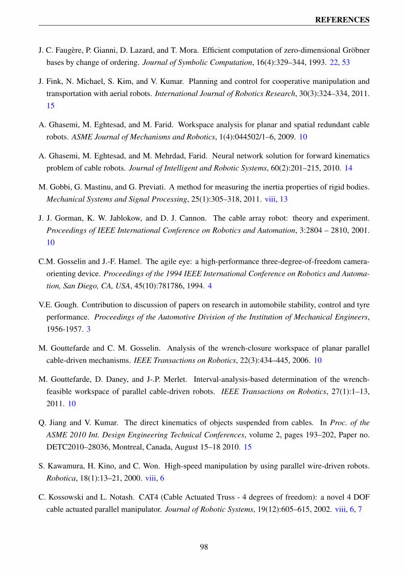
REFERENCES
J. C. Faugere, P. Gianni, D. Lazard, and T. Mora. Efficient computation of zero-dimensional Grobnerbases by change of ordering. Journal of Symbolic Computation, 16(4):329–344, 1993. 22, 53
J. Fink, N. Michael, S. Kim, and V. Kumar. Planning and control for cooperative manipulation andtransportation with aerial robots. International Journal of Robotics Research, 30(3):324–334, 2011.15
A. Ghasemi, M. Eghtesad, and M. Farid. Workspace analysis for planar and spatial redundant cablerobots. ASME Journal of Mechanisms and Robotics, 1(4):044502/1–6, 2009. 10
A. Ghasemi, M. Eghtesad, and M. Mehrdad, Farid. Neural network solution for forward kinematicsproblem of cable robots. Journal of Intelligent and Robotic Systems, 60(2):201–215, 2010. 14
M. Gobbi, G. Mastinu, and G. Previati. A method for measuring the inertia properties of rigid bodies.Mechanical Systems and Signal Processing, 25(1):305–318, 2011. viii, 13
J. J. Gorman, K. W. Jablokow, and D. J. Cannon. The cable array robot: theory and experiment.Proceedings of IEEE International Conference on Robotics and Automation, 3:2804 – 2810, 2001.10
C.M. Gosselin and J.-F. Hamel. The agile eye: a high-performance three-degree-of-freedom camera-orienting device. Proceedings of the 1994 IEEE International Conference on Robotics and Automa-
tion, San Diego, CA, USA, 45(10):781786, 1994. 4
V.E. Gough. Contribution to discussion of papers on research in automobile stability, control and tyreperformance. Proceedings of the Automotive Division of the Institution of Mechanical Engineers,1956-1957. 3
M. Gouttefarde and C. M. Gosselin. Analysis of the wrench-closure workspace of planar parallelcable-driven mechanisms. IEEE Transactions on Robotics, 22(3):434–445, 2006. 10
M. Gouttefarde, D. Daney, and J-.P. Merlet. Interval-analysis-based determination of the wrench-feasible workspace of parallel cable-driven robots. IEEE Transactions on Robotics, 27(1):1–13,2011. 10
Q. Jiang and V. Kumar. The direct kinematics of objects suspended from cables. In Proc. of the
ASME 2010 Int. Design Engineering Technical Conferences, volume 2, pages 193–202, Paper no.DETC2010–28036, Montreal, Canada, August 15–18 2010. 15
S. Kawamura, H. Kino, and C. Won. High-speed manipulation by using parallel wire-driven robots.Robotica, 18(1):13–21, 2000. viii, 6
C. Kossowski and L. Notash. CAT4 (Cable Actuated Truss - 4 degrees of freedom): a novel 4 DOFcable actuated parallel manipulator. Journal of Robotic Systems, 19(12):605–615, 2002. viii, 6, 7
98
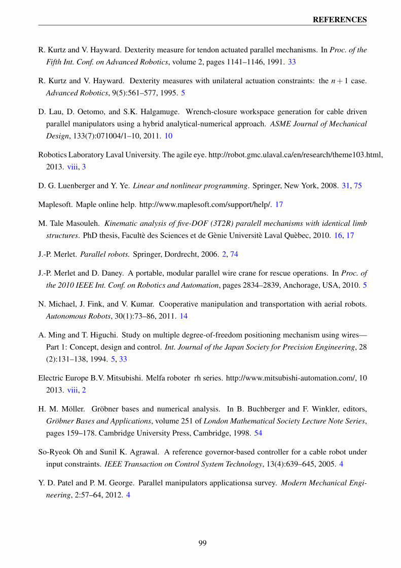
REFERENCES
R. Kurtz and V. Hayward. Dexterity measure for tendon actuated parallel mechanisms. In Proc. of the
Fifth Int. Conf. on Advanced Robotics, volume 2, pages 1141–1146, 1991. 33
R. Kurtz and V. Hayward. Dexterity measures with unilateral actuation constraints: the n+ 1 case.Advanced Robotics, 9(5):561–577, 1995. 5
D. Lau, D. Oetomo, and S.K. Halgamuge. Wrench-closure workspace generation for cable drivenparallel manipulators using a hybrid analytical-numerical approach. ASME Journal of Mechanical
Design, 133(7):071004/1–10, 2011. 10
Robotics Laboratory Laval University. The agile eye. http://robot.gmc.ulaval.ca/en/research/theme103.html,2013. viii, 3
D. G. Luenberger and Y. Ye. Linear and nonlinear programming. Springer, New York, 2008. 31, 75
Maplesoft. Maple online help. http://www.maplesoft.com/support/help/. 17
M. Tale Masouleh. Kinematic analysis of five-DOF (3T2R) paralell mechanisms with identical limb
structures. PhD thesis, Faculte des Sciences et de Genie Universite Laval Quebec, 2010. 16, 17
J.-P. Merlet. Parallel robots. Springer, Dordrecht, 2006. 2, 74
J.-P. Merlet and D. Daney. A portable, modular parallel wire crane for rescue operations. In Proc. of
the 2010 IEEE Int. Conf. on Robotics and Automation, pages 2834–2839, Anchorage, USA, 2010. 5
N. Michael, J. Fink, and V. Kumar. Cooperative manipulation and transportation with aerial robots.Autonomous Robots, 30(1):73–86, 2011. 14
A. Ming and T. Higuchi. Study on multiple degree-of-freedom positioning mechanism using wires—Part 1: Concept, design and control. Int. Journal of the Japan Society for Precision Engineering, 28(2):131–138, 1994. 5, 33
Electric Europe B.V. Mitsubishi. Melfa roboter rh series. http://www.mitsubishi-automation.com/, 102013. viii, 2
H. M. Moller. Grobner bases and numerical analysis. In B. Buchberger and F. Winkler, editors,Grobner Bases and Applications, volume 251 of London Mathematical Society Lecture Note Series,pages 159–178. Cambridge University Press, Cambridge, 1998. 54
So-Ryeok Oh and Sunil K. Agrawal. A reference governor-based controller for a cable robot underinput constraints. IEEE Transaction on Control System Technology, 13(4):639–645, 2005. 4
Y. D. Patel and P. M. George. Parallel manipulators applicationsa survey. Modern Mechanical Engi-
neering, 2:57–64, 2012. 4
99
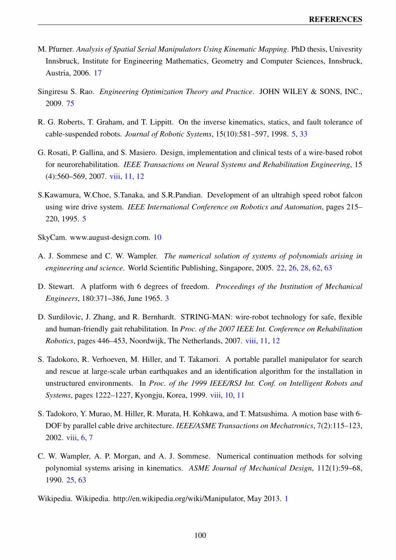
REFERENCES
M. Pfurner. Analysis of Spatial Serial Manipulators Using Kinematic Mapping. PhD thesis, UnivesrityInnsbruck, Institute for Engineering Mathematics, Geometry and Computer Sciences, Innsbruck,Austria, 2006. 17
Singiresu S. Rao. Engineering Optimization Theory and Practice. JOHN WILEY & SONS, INC.,2009. 75
R. G. Roberts, T. Graham, and T. Lippitt. On the inverse kinematics, statics, and fault tolerance ofcable-suspended robots. Journal of Robotic Systems, 15(10):581–597, 1998. 5, 33
G. Rosati, P. Gallina, and S. Masiero. Design, implementation and clinical tests of a wire-based robotfor neurorehabilitation. IEEE Transactions on Neural Systems and Rehabilitation Engineering, 15(4):560–569, 2007. viii, 11, 12
S.Kawamura, W.Choe, S.Tanaka, and S.R.Pandian. Development of an ultrahigh speed robot falconusing wire drive system. IEEE International Conference on Robotics and Automation, pages 215–220, 1995. 5
SkyCam. www.august-design.com. 10
A. J. Sommese and C. W. Wampler. The numerical solution of systems of polynomials arising in
engineering and science. World Scientific Publishing, Singapore, 2005. 22, 26, 28, 62, 63
D. Stewart. A platform with 6 degrees of freedom. Proceedings of the Institution of Mechanical
Engineers, 180:371–386, June 1965. 3
D. Surdilovic, J. Zhang, and R. Bernhardt. STRING-MAN: wire-robot technology for safe, flexibleand human-friendly gait rehabilitation. In Proc. of the 2007 IEEE Int. Conference on Rehabilitation
Robotics, pages 446–453, Noordwijk, The Netherlands, 2007. viii, 11, 12
S. Tadokoro, R. Verhoeven, M. Hiller, and T. Takamori. A portable parallel manipulator for searchand rescue at large-scale urban earthquakes and an identification algorithm for the installation inunstructured environments. In Proc. of the 1999 IEEE/RSJ Int. Conf. on Intelligent Robots and
Systems, pages 1222–1227, Kyongju, Korea, 1999. viii, 10, 11
S. Tadokoro, Y. Murao, M. Hiller, R. Murata, H. Kohkawa, and T. Matsushima. A motion base with 6-DOF by parallel cable drive architecture. IEEE/ASME Transactions on Mechatronics, 7(2):115–123,2002. viii, 6, 7
C. W. Wampler, A. P. Morgan, and A. J. Sommese. Numerical continuation methods for solvingpolynomial systems arising in kinematics. ASME Journal of Mechanical Design, 112(1):59–68,1990. 25, 63
Wikipedia. Wikipedia. http://en.wikipedia.org/wiki/Manipulator, May 2013. 1
100