MEASURING THE MARGINAL IMPACT OF CO2 EMISSIONS ON ATMOSPHERIC CONCENTRATIONS∗

Brian C. O’Neill

Current affiliation: International Institute for Applied Systems Analysis (IIASA) A-2361 Laxenburg, Austria

oneill@iiasa.ac.at

CAVEAT: This chapter was written in 1995-1996. The derivation of “convolution response

functions”, their application to the carbon cycle, and the attribution of concentrations I still stand by. It also represents a methodology for attribution that is different in some respects from those presented at the Expert Meeting on Assessment of Contributions to Climate Change in Bracknell in September 2002. However, portions of this chapter also discuss applications to Global Warming

Potentials and the calculation of marginal climate damages that I no longer support. For a number of reasons I no longer believe the new type of response

function derived in this chapter is the right tool for those jobs. An updated version of this chapter focused on the attribution methodology, and comparing it to alternative methods (such as those presented in Bracknell) by recasting them

within the theoretical framework of response functions, is in preparation.

– Brian O’Neill, October 4, 2002

∗ This manuscript was published as Chapter 3 of a 1996 Ph.D. dissertation. The full citation is: O’Neill, B.C. 1996. Measuring the marginal impact of CO2 emissions on atmospheric concentrations. In Greenhouse gases: Timescales, response functions, and the impact of population growth on future emissions, Chapter 3, pp. 65-116. Ph.D. Dissertation, New York University, New York, NY, USA.

MEASURING THE MARGINAL IMPACT OF CO2 EMISSIONS ON ATMOSPHERIC CONCENTRATIONS∗

Brian C. O’Neill

Current affiliation: International Institute for Applied Systems Analysis (IIASA) A-2361 Laxenburg, Austria

oneill@iiasa.ac.at

Abstract The response of atmospheric CO2 concentrations to an incremental increase in emissions is usually measured using an impulse response function. These functions are then used in calculating Global Warming Potentials, marginal climate damages, and CO2 timescales. It is shown here that the impulse response method implicitly double counts the effects of emissions on concentration by not properly accounting for carbon cycle nonlinearities, leading to a systematic overestimation of the persistence of the effect of an emissions pulse. A new method of determining marginal response functions is derived which accurately proportions responsibility for CO2 concentration among emissions cohorts. Results show that the new functions indicate up to a 50% reduction in the essentially irreversible fraction of the effect of a present emission. This reduced long term response leads to a 20-30% reduction in 500-year Global Warming Potentials and a 10-15% reduction in climate damages per ton of emission. The new functions are also applied to historical emissions, and indicate that emissions from developed countries are responsible for approximately 75% of the present excess atmospheric CO2 concentration. Introduction Response functions for greenhouse gases describe the effect of emissions pulses on atmospheric concentrations through time. They play a fundamental role in determining the relative Global Warming Potentials (GWPs) and marginal economic damages associated with emissions of different greenhouse gases. Marginal damages and GWPs are, in turn, important tools for assessing the costs and benefits of emissions reduction strategies and of estimating on economic grounds the appropriate policy response to potential future warming. Response functions for CO2 were originally based on unbalanced carbon cycle models lacking a representation of the terrestrial biosphere (Maier-Reimer and Hasselmann, 1987; Siegenthaler and Oeschger, 1987; Watson et al., 1990). These functions were used to approximate the atmospheric response to emissions under any emissions scenario by assuming linear behavior of the carbon cycle. Subsequent work (Caldeira and Kasting, 1993) showed that when nonlinearities in ocean uptake were taken into account, response functions were extremely sensitive to future emissions. However,

∗ This manuscript was published as Chapter 3 of a 1996 Ph.D. dissertation. The full citation is: O’Neill, B.C. 1996. Measuring the marginal impact of CO2 emissions on atmospheric concentrations. In Greenhouse gases: Timescales, response functions, and the impact of population growth on future emissions, Chapter 3, pp. 65-116. Ph.D. Dissertation, New York University, New York, NY, USA.

nonlinearities in CO2 radiative forcing essentially compensate for the effect. As a result, the time-integrated radiative forcing associated with a pulse (i.e., its warming potential) was shown to be relatively independent of the emissions scenario. The importance of the terrestrial biosphere to CO2 uptake was not fully appreciated until later (Moore and Braswell, 1994; Kheshgi et al., 1994). More recent IPCC reports (Houghton et al., 1995 and in press) have calculated GWPs using carbon cycle models balanced by the assumption of CO2 fertilization of the biosphere. Incorporation of this biospheric uptake reduced the integrated forcing implied by CO2 emissions, systematically raising the GWPs of other gases (measured relative to CO2) by 20 - 30% (Albritton, 1995). Response functions from balanced carbon cycle models were shown to be insensitive in the short term to the nature of carbon sinks and to the assumed emissions scenario (Moore and Braswell, 1994; Gaffin et al., 1995). Long-term response remained quite sensitive to emissions, but again it was found that reduced radiative forcing at higher CO2 levels compensated for reduced oceanic uptake, so that integrated forcing under various scenarios varied by no more than ±20% (Albritton, 1995). This study shows that even response functions derived from current balanced carbon cycle models do not accurately measure the effect of emissions on concentrations. Although such models incorporate nonlinearities in exchange fluxes between reservoirs, the method commonly used to derive the response function from the model does not fully account for nonlinear interactions between emissions pulses. As a result, some of the effect assigned to a particular emission is implicitly "double counted", leading to a systematic overestimation independent of the emissions scenario. A new method for accurately determining response functions in nonlinear systems is derived and applied to a carbon cycle model. Corrected response functions are calculated for high and low future emissions scenarios, and are shown to reduce the 500-year integrated forcing resulting from a CO2 emissions pulse by 20-30%. Reductions over the 20- and 100-year horizons also used in GWPs are negligible. Most economic studies employing response functions (e.g., Fankhauser, 1994; Nordhaus, 1991) use a linear, often ocean-only response (Maier-Reimer and Hasselmann, 1987). To investigate the importance of this shortcoming, this study quantifies the changes in marginal damage estimates resulting from replacing ocean-only response functions with those based on balanced carbon cycle models, and also with the corrected response functions derived here. Damages will not necessarily change in the same manner as GWPs when based on improved response functions since damages are calculated as a nonlinear function of temperature, whereas GWPs only measure integrated radiative forcing. Kheshgi et al. (1994) have, in fact, pointed out that biospheric uptake may be especially important to economic assessments since it significantly reduces the impact on concentration in the first few decades following an emission. Since damage functions commonly discount the future, reductions in the short-term response would be expected to have a greater impact than reductions in the long-term response. Results show that use of the corrected response function derived here reduces damage estimates by 10 - 15% relative to those determined with ocean-only responses. Damages calculated using functions determined from balanced models, but still subject to "double counting", are generally intermediate between the two; under conditions of high

future emissions and a low discount rate, however, they yield damages higher than the corrected method by over 20%. Because the new response functions accurately proportion responsibility for concentrations to emissions pulses, they also provide the best basis for tracking the fate of emissions. The fate of past regional CO2 emissions is tracked to determine the relative regional shares of responsibility for the current atmospheric CO2 excess, an issue important to determining equitable emissions reduction strategies. It is shown that global emissions since 1950 account for 72% of the current excess. By assuming that pre-1950 emissions were largely from the developed world, it is estimated that roughly three-quarters of the current excess is due to emission from more developed countries and one quarter from less developed countries. Marginal impacts of emissions The most prominent index of the marginal impact of emissions on radiative forcing is the Global Warming Potential (Albritton, 1995). GWPs compare the relative effects of emissions on climate forcing without attempting to trace them through to climate change and resulting damages. A forceful case against the use of strictly physical indexes has been made by several economists (Schmalensee, 1993; Eckhaus, 1992; Victor) who have argued that economic policy decisions must be based on measures which incorporate climate impacts. Economists have therefore calculated marginal damage costs of emissions using two methods. Optimal control studies (Nordhaus, 1992; Peck and Tiesberg, 1992) calculate marginal damages as the shadow price of emissions along a socially optimal emissions path. Although this type of modeling framework must include some type of (usually simplified) gas-cycle and climate sub-model, it does not require an explicit, separately determined measure of the marginal impact of emissions on concentrations. Instead, the marginal damages are implicit in the optimization routine, since the optimal solution by definition will have the property that the chosen marginal tax rate will equal marginal damages. As an alternative, marginal damage costs can be calculated within a non-optimal economic model. This method has the advantage that while it can incorporate essential economic concepts missing from physical indexes, it is not limited to optimal emissions trajectories but can be applied to any specified emissions path. Such calculations require greenhouse gas cycle and climate model results to explicitly describe the marginal effect of emissions on concentrations and climate under different scenarios of future emissions, a need commonly filled by "impulse response" functions. The factors leading to marginal damages can be usefully disaggregated in the following way (eqs. (1-3) below follow closely Schmalensee (1993) and Fankhauser (1994)). Assume a base scenario consisting of historical emissions and some projection of future emissions of a greenhouse gas i. Let MDi(t,I(t)) represent the present value of the discounted sum of future damages resulting from an incremental change in emissions of gas i at time t. The term is also written as a function of the magnitude (I) of emissions at time t in the base scenario, which will be useful later. If the change in damages through time following a change in emissions at time to is ∂D(t)/∂I(to), then

dtetItDtItMD t

t oioioi

o

δ

∂∂ −

∞

∫=)()())(,( (1)

where δ is the discount rate. However, damages result only indirectly from emissions, so the damage derivative on the right hand side of eq. (1) must be traced through several other factors: ∂Mi(s)/∂Ii(to) the change in the atmospheric concentration (or mass) of gas i at

time s due to a change in emissions at time to, where s ≥ to ∂R(s)/∂Mi(s) the change in radiative forcing caused by a change in the

concentration of gas i ∂T(t)/∂R(s) the change in temperature at time t due to a change in radiative

forcing at time s, where t ≥ s ∂D(t)/∂T(t) the change in damages due to a change in temperature Note that the derivatives of damages and radiative forcing at a particular time are assumed to be caused by changes in temperature and concentration occurring at the same time. In contrast, the derivatives of concentration and temperature describe changes in these variables due to changes in emissions and radiative forcing that took place at the same time or in the past. This characteristic results from the fact that greenhouse gas emissions are not removed immediately from the atmosphere but affect concentrations well into the future; similarly, a change in radiative forcing will be expressed as a temperature change over a period of time in the future due to thermal lags in the climate system. Combining all of these terms, the damage derivative in eq. (1) can be expanded to:

dstIsM

sMsR

sRtT

tTtD

tItD t

t oi

i

ioi o

∫

=

)()(

)()(

)()(

)()(

)()(

∂∂

∂∂

∂∂

∂∂

∂∂

(2)

The integral on the right hand side is necessary since temperature at time t is a function of the history of radiative forcing, and not simply of the radiative forcing at time t. Eq. (2) gives the following more comprehensive equation for marginal damages:

dtedstIsM

sMsR

sRtT

tTtDtItMD t

t

t

t oi

i

ioioi

o o

δ

∂∂

∂∂

∂∂

∂∂ −

∞

∫ ∫

=

)()(

)()(

)()(

)()())(,( (3)

Eq. (3) summarizes the biogeochemical, climatological, and economic processes which must be accounted for in marginal damage estimates. Compare this equation with

the Global Warming Potential index, which is written as the Absolute Global Warming Potential (AGWP) of one gas relative to that of CO2 where the AGWP is:

dttItM

tMtRtItAGWP

ot oi

i

ioioi ∫

∞

=

)()(

)()())(,(

∂∂

∂∂

(4)

Both this formulation and a modified approach which includes a discounting term (Lashof and Ahuja, 1990) have been criticized as insufficient bases for economic decisions because of the terms included in eq. (3) but missing from eq. (4) (Schmalensee, 1993; Eckhaus, 1992). However, use of eq. (3) demands that special consideration be given to the marginal response functions commonly used to define the effect of a small change in emissions on concentration. In particular, eq. (3) demands that estimates for each term in the equation be made in a manner consistent with the economic definition of a marginal damage. The definition of a marginal effect (marginal cost, marginal damage, marginal utility, etc.) is the extra effect resulting from the addition of one more unit of the cause (Samuelson and Nordhaus, 1985). For example, marginal cost of production is the extra total cost resulting from one additional unit of output. By definition, the sum of the marginal costs of each of the units produced must equal the total cost. Translating to CO2, where emissions are the cause and atmospheric concentrations the effect, the marginal effect of an emission is the extra concentration resulting from one additional unit of emissions. And the marginal effect of each unit of emissions, summed over all emissions, must equal the total concentration. Applied to marginal damages, the definition requires that the sum of marginal damages due to each increment of emissions in a particular time period must equal the total damage due to the whole emission in that time period, or

∫=)(

0

),()(otI

oioi dtMDtTD εε (5)

where TDi(to) is the present value of the total damage caused by the amount of gas i emitted at time to. In addition, the damage due to emissions in each time period must sum to the cumulative total damages over the entire scenario, once all damage costs are valued relative to the same time period using the same discount rate. That is, the base scenario will generate damages to the economy over time due to the time path of the concentration of gas i. Eqs. (3) and (5) divide responsibility for this damage among cohorts of the emissions function. If the discount rate is set to zero so that all damages are measured in terms of their full value at the time at which they occur, then cumulative total damages (CTD) are

∫=t

ii dTDtCTD0

)()( ττ (6)

The question therefore is: does the method of determining marginal damages guarantee that the sum of the damages attributable to each increment of emissions will equal total damages? That is, does eq. (3) guarantee that eqs. (5) and (6) hold? If the system described by eq. (3) is linear, eqs. (5) and (6) hold since the effect of each emissions increment would be independent of all other emissions. This is essentially a statement of the superposition principle characteristic of linear systems, which guarantees that the derivative terms in eq. (3), when integrated in eqs. (5) and (6), will add up to the total changes in each variable. However, as previously discussed, eq. (3) contains two kinds of nonlinearities manifested as two different types of derivatives: those evaluated instantaneously and those whose influence stretches over time. The difference is crucial, since nonlinearities in instantaneous derivatives are compatible with marginal calculations, while nonlinearities operating over time are not. For example, the cost of a unit of production is often a nonlinear function of the number of units produced, a situation described by increasing or decreasing returns to scale. However, the full marginal cost of each unit is typically incorporated into the total cost curve at the time of its production and is independent of subsequent production levels. Total costs are therefore still equal to the sum of marginal costs determined by calculating the difference in total cost before and after producing an extra unit of output. The same principle applies to the instantaneous derivatives in eq. (2). Changes in damages through time (∂D/∂t), for example, can be unambiguously attributed to changes in temperature occurring at the same time (∂T/∂t). Therefore when the derivative ∂D/∂T is integrated over time, it will always accurately assign responsibility for a change in damages to its cause: a simultaneous change in temperature. The same holds true for the radiative forcing derivative, ∂R(t)/∂Mi(t). However, changes in concentration through time (∂M/∂t) are the result of an entire emissions history which is undergoing removal. If removal is nonlinear, the effect of an incremental increase in emissions will be determined partly by future emissions, and the effect of those future emissions will be determined partly by the incremental increase. As a result, the measured concentration change following an emissions impulse is not due entirely to the impulse itself, but also to the presence of other emissions cohorts. The impulse response method of determining marginal effects, however, assigns all of the responsibility to the incremental emissions increase. It therefore implicitly double counts effects. Before demonstrating this shortcoming formally, it is important to point out that the temperature response to changes in radiative forcing (∂T(t)/∂R(s)) has the same potential for nonlinear interactions. Temperature depends on radiative forcing through both the equilibrium climate sensitivity, which describes the eventual magnitude of the temperature change caused by a change in radiative forcing, and the thermal inertia of the climate system, which will delay the time at which the equilibrium sensitivity is realized. If the effect of a radiative forcing change at time to can be modified by and in turn modify the effect of past or subsequent changes in radiative forcing, then a change in temperature cannot be easily ascribed to one particular change in radiative forcing. Although this type of nonlinearity is a distinct possibility in the case of temperature response, both equilibrium climate sensitivity and thermal inertia processes

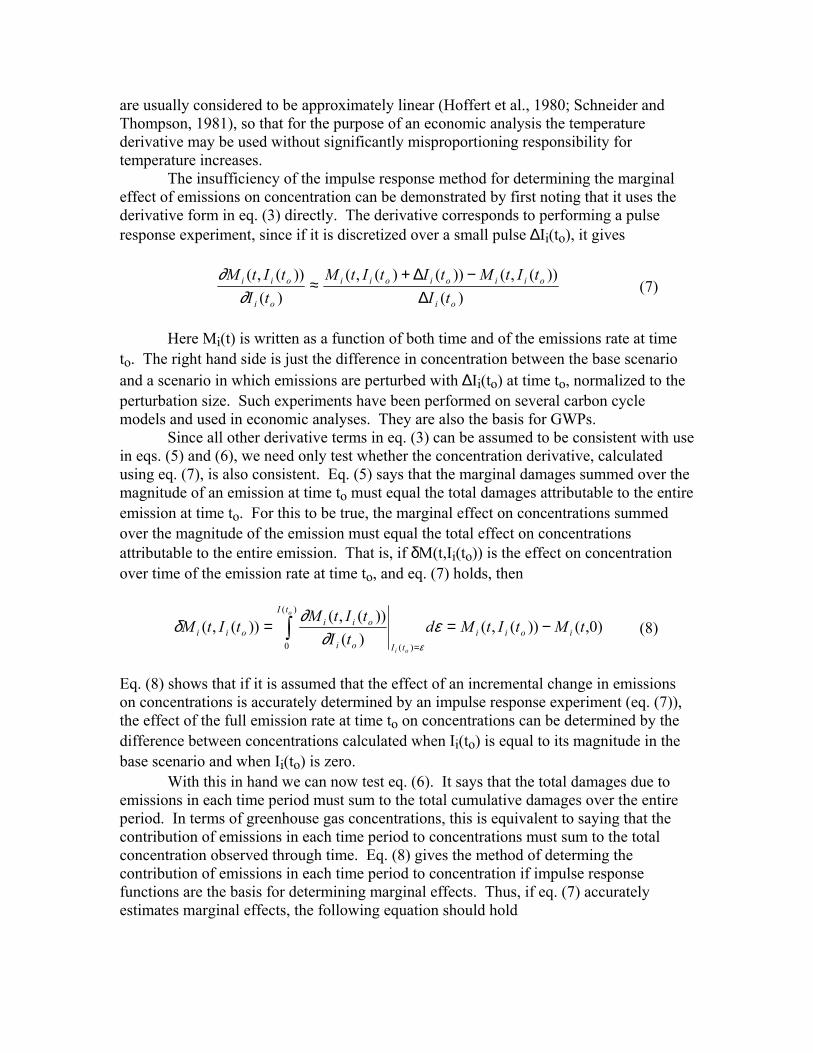
are usually considered to be approximately linear (Hoffert et al., 1980; Schneider and Thompson, 1981), so that for the purpose of an economic analysis the temperature derivative may be used without significantly misproportioning responsibility for temperature increases. The insufficiency of the impulse response method for determining the marginal effect of emissions on concentration can be demonstrated by first noting that it uses the derivative form in eq. (3) directly. The derivative corresponds to performing a pulse response experiment, since if it is discretized over a small pulse ∆Ii(to), it gives

)(

))(,())()(,()(

))(,(

oi

oiioioii

oi

oii

tItItMtItItM

tItItM

∆−∆+

≈∂

∂ (7)

Here Mi(t) is written as a function of both time and of the emissions rate at time to. The right hand side is just the difference in concentration between the base scenario and a scenario in which emissions are perturbed with ∆Ii(to) at time to, normalized to the perturbation size. Such experiments have been performed on several carbon cycle models and used in economic analyses. They are also the basis for GWPs. Since all other derivative terms in eq. (3) can be assumed to be consistent with use in eqs. (5) and (6), we need only test whether the concentration derivative, calculated using eq. (7), is also consistent. Eq. (5) says that the marginal damages summed over the magnitude of an emission at time to must equal the total damages attributable to the entire emission at time to. For this to be true, the marginal effect on concentrations summed over the magnitude of the emission must equal the total effect on concentrations attributable to the entire emission. That is, if δM(t,Ii(to)) is the effect on concentration over time of the emission rate at time to, and eq. (7) holds, then

)0,())(,()(

))(,())(,(

)(

)(

0

tMtItMdtI

tItMtItM ioii

tI

tI

oi

oiioii

oi

o

−===

∫ ε∂

∂δε

(8)

Eq. (8) shows that if it is assumed that the effect of an incremental change in emissions on concentrations is accurately determined by an impulse response experiment (eq. (7)), the effect of the full emission rate at time to on concentrations can be determined by the difference between concentrations calculated when Ii(to) is equal to its magnitude in the base scenario and when Ii(to) is zero. With this in hand we can now test eq. (6). It says that the total damages due to emissions in each time period must sum to the total cumulative damages over the entire period. In terms of greenhouse gas concentrations, this is equivalent to saying that the contribution of emissions in each time period to concentrations must sum to the total concentration observed through time. Eq. (8) gives the method of determing the contribution of emissions in each time period to concentration if impulse response functions are the basis for determining marginal effects. Thus, if eq. (7) accurately estimates marginal effects, the following equation should hold

( )∫ ′′−′=∆t

iii tdttItMtM0

)(,)( δ (9)

where ∆Mi(t) is the concentration of gas i in excess of its equilibrium concentration (i.e., the concentration resulting from the anthropogenic emissions forcing). Figure 1 shows the results of such a test for a standard carbon cycle model. Clearly, eq. (9) does not reproduce the observed path of ∆M(t). The reason is that the impulse response experiment does not accurately estimate the marginal response function due to inherent nonlinearities in the system which lead to double counting. Eq. (7) therefore overestimates the contribution of any particular emissions increment. The following two sections develop a new method for determining response functions in nonlinear systems by equitably proportioning responsibility for concentration increases among emissions cohorts. The first section examines a single reservoir system, for clarity, before extending results in the second section to a multi-reservoir system. The last section then applies these results to a carbon cycle model to determine new, accurate response functions, applies the response functions to the calculation of absolute GWPs for CO2 and to marginal damage estimates, and examines the sensitivity of the results to the assumed base scenario. Single well-mixed reservoir with a nonlinear removal flux Consider a system consisting of a single well-mixed reservoir with a constant natural influx In and a removal flux F(t). At equilibrium, F(t) = Feq = In. Although in principle F could be a function of any number of variables either endogenous or exogenous to the system, it can always be written in a mathematically equivalent form as a removal rate k multiplied by the reservoir contents M. Because the reservoir is well-mixed, this representation has the special property of describing removal in terms of the probability per unit time (k) of any particular unit of mass being removed from the reservoir. Therefore not only will k (multiplied by M) transfer the correct amount of bulk mass out of the reservoir, it will also remove the correct proportion of any tracer mass to which it is applied. At equilibrium, eqeqn MkI −=0 (10) If the reservoir is forced with a time-dependent anthropogenic input as well, the equation describing the evolution of reservoir mass is

)()()()( tMtktIItM an −+=•

(11) where the overdot indicates a derivative with respect to time, and the removal flux is again written as a removal probability per unit time multiplied by the reservoir contents. Note that although in principle k could have any number of functional forms, it is expressed as a function of time alone. This is not meant to indicate that k is strictly a

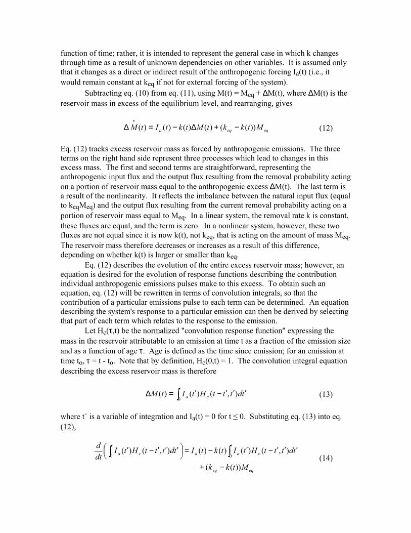
function of time; rather, it is intended to represent the general case in which k changes through time as a result of unknown dependencies on other variables. It is assumed only that it changes as a direct or indirect result of the anthropogenic forcing Ia(t) (i.e., it would remain constant at keq if not for external forcing of the system). Subtracting eq. (10) from eq. (11), using M(t) = Meq + ∆M(t), where ∆M(t) is the reservoir mass in excess of the equilibrium level, and rearranging, gives

eqeqa MtkktMtktItM ))(()()()()( −+∆−=∆•

(12) Eq. (12) tracks excess reservoir mass as forced by anthropogenic emissions. The three terms on the right hand side represent three processes which lead to changes in this excess mass. The first and second terms are straightforward, representing the anthropogenic input flux and the output flux resulting from the removal probability acting on a portion of reservoir mass equal to the anthropogenic excess ∆M(t). The last term is a result of the nonlinearity. It reflects the imbalance between the natural input flux (equal to keqMeq) and the output flux resulting from the current removal probability acting on a portion of reservoir mass equal to Meq. In a linear system, the removal rate k is constant, these fluxes are equal, and the term is zero. In a nonlinear system, however, these two fluxes are not equal since it is now k(t), not keq, that is acting on the amount of mass Meq. The reservoir mass therefore decreases or increases as a result of this difference, depending on whether k(t) is larger or smaller than keq. Eq. (12) describes the evolution of the entire excess reservoir mass; however, an equation is desired for the evolution of response functions describing the contribution individual anthropogenic emissions pulses make to this excess. To obtain such an equation, eq. (12) will be rewritten in terms of convolution integrals, so that the contribution of a particular emissions pulse to each term can be determined. An equation describing the system's response to a particular emission can then be derived by selecting that part of each term which relates to the response to the emission. Let Hc(τ,t) be the normalized "convolution response function" expressing the mass in the reservoir attributable to an emission at time t as a fraction of the emission size and as a function of age τ. Age is defined as the time since emission; for an emission at time to, τ = t - to. Note that by definition, Hc(0,t) = 1. The convolution integral equation describing the excess reservoir mass is therefore

∫ ′′′−′=∆t

ca tdtttHtItM0

),()()( (13) where t´ is a variable of integration and Ia(t) = 0 for t ≤ 0. Substituting eq. (13) into eq. (12),

eqeq

t

caa

t

ca

Mtkk

tdtttHtItktItdtttHtIdtd

))((

),()()()(),()(00

−+

′′′−′−=

′′′−′ ∫∫ (14)

Taking the derivative on the left hand side and using Hc(0,t) = 1 gives

( ) eqeq

t

ca

t

ca MtkkdtHItkdtHIdtd ))((),()()(),()(

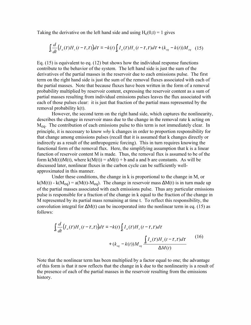
00−+−−=− ∫∫ ττττττττ (15)

Eq. (15) is equivalent to eq. (12) but shows how the individual response functions contribute to the behavior of the system. The left hand side is just the sum of the derivatives of the partial masses in the reservoir due to each emissions pulse. The first term on the right hand side is just the sum of the removal fluxes associated with each of the partial masses. Note that because fluxes have been written in the form of a removal probability multiplied by reservoir content, expressing the reservoir content as a sum of partial masses resulting from individual emissions pulses leaves the flux associated with each of those pulses clear: it is just that fraction of the partial mass represented by the removal probability k(t). However, the second term on the right hand side, which captures the nonlinearity, describes the change in reservoir mass due to the change in the removal rate k acting on Meq. The contribution of each emissions pulse to this term is not immediately clear. In principle, it is necessary to know why k changes in order to proportion responsibility for that change among emissions pulses (recall that it is assumed that k changes directly or indirectly as a result of the anthropogenic forcing). This in turn requires knowing the functional form of the removal flux. Here, the simplifying assumption that k is a linear function of reservoir content M is made. Thus, the removal flux is assumed to be of the form k(M(t))M(t), where k(M(t)) = aM(t) + b and a and b are constants. As will be discussed later, nonlinear fluxes in the carbon cycle can be sufficiently well-approximated in this manner. Under these conditions, the change in k is proportional to the change in M, or k(M(t)) - k(Meq) = a(M(t)-Meq). The change in reservoir mass ∆M(t) is in turn made up of the partial masses associated with each emissions pulse. Thus any particular emissions pulse is responsible for a fraction of the change in k equal to the fraction of the change in M represented by its partial mass remaining at time t. To reflect this responsibility, the convolution integral for ∆M(t) can be incorporated into the nonlinear term in eq. (15) as follows:

( )

)(

),()())((

),()()(),()(

0

00

tM

dtHIMtkk

dtHItkdtHIdtd

t

ca

eqeq

t

ca

t

ca

∆

−−+

−−=−

∫

∫∫ττττ

ττττττττ

(16)

Note that the nonlinear term has been multiplied by a factor equal to one; the advantage of this form is that it now reflects that the change in k due to the nonlinearity is a result of the presence of each of the partial masses in the reservoir resulting from the emissions history.

Eq. (16) can be used to derive a general equation describing the response functions Hc(τ,t) by first converting it from continuous to discrete form; i.e., by writing it in terms of summations of responses to a finite number of emissions pulses:

( )

)(

),()())((

),()()(),()(

,...,0

,...,0,...,0

tM

ttttHtIMtkk

ttttHtItkttttHtIdtd

t

ttca

eqeq

t

ttca

t

ttca

∆

′∆′′−′−+

′∆′′−′−=′∆′′−′

∑

∑∑

′∆=′

′∆=′′∆=′

(17)

In this form, eq. (17) describes the evolution of the reservoir mass as an explicit sum of responses to emissions pulses at times t´ = 0, ∆t´, etc. In the limit as ∆t´ tends to 0, eq. (17) is identical to eq. (16). A general equation for a single response function can be found by letting t´ = to, which selects the one term from each of the summations corresponding to the emission at time to:

( )

)(),()(

))((

),()()(),()(

tMttttHtI

Mtkk

ttttHtItkttttHtIdtd

oocoaeqeq

oocoaoocoa

∆′∆−

−+

′∆−−=′∆− (18)

Since it is more natural to describe the evolution of a response function in terms of age (time since emission) than in terms of time, the relations τ = t - to and dτ = dt are used, which, along with some simplification, gives

),()(

))(()(),( oco

eqoeqooc tH

tMM

tkktktHdd τ

ττττ

τ

+∆

+−−+−= (19)

Eq. (19) is a general differential equation for the response function Hc(τ,to) with initial condition Ηc(0,to) = 1. It shows that the response to an emission consists of removal by the reservoir removal rate and, in addition, a buildup or drawdown of reservoir mass due to the change in k caused by nonlinearities. Eq. (19) can be solved for a convolution response function corresponding to any particular emission as long as M(t) and k(t) are known. Fig. 2 demonstrates the application of eq. (19) to a hypothetical single well-mixed reservoir. The analytical solution is reproduced by the convolution of the anthropogenic emissions function with the convolution response functions. A convolution using response functions based on suppressing each emissions pulse in turn, however, significantly overestimates the evolution of the total reservoir mass. As discussed in the previous section, this method would only have successfully reproduced reservoir mass if the impulse response method correctly determined marginal responses in nonlinear systems.

Recall that the goal of the exercise is to find a function describing the marginal effect of an additional emission to the system, not the effect of the full emission in a particular time period as given by Hc(τ,t). However, under the assumption made above that k is a linear function of M, the two responses are identical. That is, the system responds proportionally to each subcomponent of the total amount of mass emitted into the reservoir over one time period ∆t, so that Hc represents the normalized response to the whole emission and to the last increment of emissions. It therefore represents the marginal response of the system. Although this response will be dependent on pulse size, this effect can be minimized by decreasing the time step ∆t so that the mass injected at each time is small. Note also that the approximation that k is a linear function of M, even if not exact, will not lead to a violation of the superposition property of the response functions. That is, even in a system in which k is nonlinear in M, or is a function of some other variable, if convolution responses to each emission in a scenario are determined using the linear k(M) approximation, the response functions will successfully reproduce the total reservoir mass when convolved with emissions. This property is assured because the changes in k assigned to each response function described by eq. (19) will always sum to the total change in k. However, the contributions of some emissions would be overestimated while those of others would be underestimated, in proportion to the accuracy of the approximation. Finally, note that if the system is linear, k is constant and eq. (19) reduces to

),(),( ococ tkHtHdd τττ

−= (20)

In this case Hc(τ,t) would be a single exponential decay curve that was constant across all emissions, as would be expected in a linear system. Multiple well-mixed reservoirs with nonlinear fluxes Consider now a multiple reservoir system containing N interconnected, well-mixed reservoirs. Assume that, as in the single-reservoir case, all fluxes from reservoir i to j are written as kij(t)Mi(t) regardless of their actual functional form. At equilibrium, the equation for reservoir i is

( )∑≠

−=N

ijeqieqijeqjeqji MkMk ,,,,0 (21)

Assume now that reservoir i is subjected to a time-dependent anthropogenic forcing. Its equation becomes

( )∑≠

•−+=

N

ijiijjjiaii tMtktMtktItM )()()()()()( , (22)

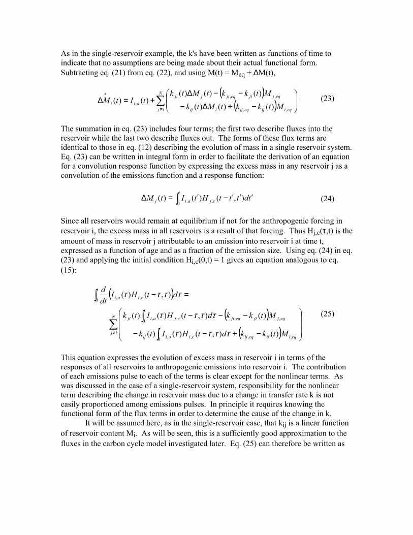
As in the single-reservoir example, the k's have been written as functions of time to indicate that no assumptions are being made about their actual functional form. Subtracting eq. (21) from eq. (22), and using M(t) = Meq + ∆M(t),

( )( )∑

≠

•

−+∆−

−−∆+=∆

N

ij eqiijeqijiij

eqjjieqjijjiaii MtkktMtk

MtkktMtktItM

,,

,,, )()()(

)()()()()( (23)

The summation in eq. (23) includes four terms; the first two describe fluxes into the reservoir while the last two describe fluxes out. The forms of these flux terms are identical to those in eq. (12) describing the evolution of mass in a single reservoir system. Eq. (23) can be written in integral form in order to facilitate the derivation of an equation for a convolution response function by expressing the excess mass in any reservoir j as a convolution of the emissions function and a response function:

∫ ′′′−′=∆t

cjaij tdtttHtItM0 ,, ),()()( (24)

Since all reservoirs would remain at equilibrium if not for the anthropogenic forcing in reservoir i, the excess mass in all reservoirs is a result of that forcing. Thus Hj,c(τ,t) is the amount of mass in reservoir j attributable to an emission into reservoir i at time t, expressed as a function of age and as a fraction of the emission size. Using eq. (24) in eq. (23) and applying the initial condition Hi,c(0,t) = 1 gives an equation analogous to eq. (15):

( )

( )( )∑

∫∫

∫

≠

−+−−

−−−

=−

N

ijeqiijeqij

t

ciaiij

eqjjieqji

t

cjaiji

t

ciai

MtkkdtHItk

MtkkdtHItk

dtHIdtd

,,0 ,,

,,0 ,,

0 ,,

)(),()()(

)(),()()(

),()(

ττττ

ττττ

ττττ

(25)

This equation expresses the evolution of excess mass in reservoir i in terms of the responses of all reservoirs to anthropogenic emissions into reservoir i. The contribution of each emissions pulse to each of the terms is clear except for the nonlinear terms. As was discussed in the case of a single-reservoir system, responsibility for the nonlinear term describing the change in reservoir mass due to a change in transfer rate k is not easily proportioned among emissions pulses. In principle it requires knowing the functional form of the flux terms in order to determine the cause of the change in k. It will be assumed here, as in the single-reservoir case, that kij is a linear function of reservoir content Mi. As will be seen, this is a sufficiently good approximation to the fluxes in the carbon cycle model investigated later. Eq. (25) can therefore be written as

( )

( )

( )

∑

∫∫

∫∫

∫

≠

∆

−−+

−−

∆

−−−

−

=−

N

ij

i

t

ciai

eqiijeqij

t

ciaiij

j

t

cjai

eqjjieqji

t

cjaiji

t

ciai

tM

dtHIMtkk

dtHItk

tM

dtHIMtkk

dtHItk

dtHIdtd

)(

),()()(

),()()(

)(

),()()(

),()()(

),()(

0 ,,

,,

0 ,,

0 ,,

,,

0 ,,

0 ,,

ττττ

ττττ

ττττ

ττττ

ττττ

(26)

To derive an equation for the response of reservoir i to an emissions pulse at a particular time, eq. (26) is first converted to discrete form:

( )

( )

( )

∑

∑

∑

∑

∑

∑

≠

′∆=′

′∆=′

′∆=′

′∆=′

′∆=′

∆

′∆′′−′−+

′∆′′−′−

∆

′∆′′−′−−

′∆′′−′

=′∆′′−′

N

ij

i

t

ttciai

eqiijeqij

t

ttciaiij

j

t

ttcjai

eqjjieqji

t

ttcjaiji

t

ttciai

tM

ttttHtIMtkk

ttttHtItk

tM

ttttHtIMtkk

ttttHtItk

ttttHtIdtd

)(

),()()(

),()()(

)(

),()()(

),()()(

),()(

,...,0,,

,,

,...,0,,

,...,0,,

,,

,...,0,,

,...,0,,

(27)

An equation for a particular response function can now be written by letting t´ = to and using τ = t - to, dτ = dt:

( ) ( )( )

( ) ( )( )∑

≠

+∆

+−−+−

+∆+−−+

=

N

ij

ocioi

eqioijeqijoij

ocjoj

eqjojieqjioji

oci

tHtM

Mtkktk

tHtM

Mtkktk

tHdd

),()(

),()(

),(

,,

,

,,

,

,

ττ

ττ

ττ

ττ

ττ

(28)

Eq. (28) is a general differential equation for the response function Hi,c(τ,t). Note that it is analogous to eq. (19), the result obtained for a single reservoir, except that it includes a return flux as well as a removal flux, and the terms are summed over all the reservoirs to which reservoir i is connected. The solution requires solving a set of simultaneous equations for all the convolution response functions Hj,c (each of which has a corresponding equation of the same form as eq. (28)) using the initial conditions Hj,c(0,t) = 0 except when j = i, in which case Hi,c(0,t) = 1. The method is therefore analogous to solving for the spread of a tracer through the system, except that the exchange fluxes described by eq. (28) do not correspond exactly to those that would be used for an ideal tracer. Eq. (28) can now be used to solve for the convolution response to an emission into a multi-box model. As an example, Fig. 3 shows the results of a nonlinear two-box model forced with anthropogenic emissions. Response functions determined using eq. (28), when convolved with emissions, accurately reproduce the mass in both reservoirs. Response functions determined by suppressing each emission into reservoir 1 in turn, when convolved with emissions, significantly overestimate reservoir mass. Application to the carbon cycle A globally aggregated carbon cycle model (fully documented in Jain et al. (1995) and Kheshgi et al. (1994)) incorporating nonlinearities in ocean uptake (through the oceanic buffer factor) and biospheric uptake (through CO2 fertilization) was constructed and tuned to match historical atmospheric CO2 data by adjusting the fertilization factor such that net land use emissions totaled 16 GtC over the decade of the 1980s. Possible temperature feedbacks in biospheric fluxes were ignored. As previously discussed, convolution response functions are calculated in the model assuming that transfer coefficients are linear functions of reservoir size. All model fluxes are in fact linear except fluxes from the atmosphere into the photosynthetic reservoirs of the terrestrial biosphere and the flux from the ocean mixed layer into the atmosphere. Photosynthetic fluxes are of the form ( ) ( ) )()()()()( 2 tMtMtMtMtF papaap ρυ += (30) where Fap is the flux from the atmosphere to the photosynthetic reservoir, Ma and Mp are the carbon masses of the atmosphere and photosynthetic reservoir, respectively, and ρ and υ are factors which account for CO2 fertilization. Thus a photosynthetic flux depends not only on the donor reservoir (Ma), but also on the receptor reservoir (Mp). The fraction of this flux which is assigned to each convolution response function (see eq. (26)) should therefore be determined by the fraction of the excess mass in the photosynthetic reservoir represented by the partial mass due to a particular emission as well as the fraction of the excess in the atmosphere represented by the corresponding partial mass in that reservoir. To first approximation, however, these two fractions are taken to be roughly equal. That is, if a particular emission is responsible for, say, 2% of the atmospheric excess at some time t, it is assumed that it is also responsible for about 2% of the excess in the photosynthetic reservoirs at time t. This approximation is

assumed to be reasonably good since photosynthetic reservoirs have short turnover times (a few years) and are therefore closely coupled to the atmosphere. When solving for the convolution response functions, eq. (30) is therefore rewritten as )()()( tMtktF aapap = (31) Fig. 4A shows that the linear assumption for kap(t) for fluxes to both photosynthetic reservoirs provides a rough first-order approximation to the actual functional dependence resulting from emissions scenarios used in this study. The approximation is quite good for low emissions scenarios and less so for higher emissions scenarios. Likewise, Fig. 4B shows that the flux from the mixed layer into the atmosphere, which is controlled by nonlinear ocean chemistry, can be converted into a similar form in which the transfer coefficient is roughly linear in the mass of carbon in the mixed layer. Again the assumption of linearity is an excellent approximation for low emissions scenarios and becomes less good for higher emissions. As noted previously, even if the approximation is not exact it will not lead to the kind of double counting errors characteristic of impulse response methods; rather, some response functions will be more heavily weighted relative to others than they would if a better approximation were used. The model was solved by calculating all fluxes in the usual manner, and then converting them to an equivalent form consisting of a transfer coefficient kij(t) multiplied by the donor reservoir content Mi(t), as outlined in the previous two sections. Convolution response functions for anthropogenic emissions over the period 1765 - 1990 were calculated using eq. (29). When convolved with emissions, these response functions reproduced the observed historical CO2 levels to which the model was tuned (see Fig. 1) to within the precision of the model calculations, providing a check that response functions were being correctly calculated. The model was then used to calculate both impulse response functions and convolution response functions in 1990 for two different future emissions scenarios: the IS92a and IS92c business as usual scenarios describing high and low potential emissions paths over the next century. Both scenarios were extended for several hundred years into the future as shown in Fig. 5A (and as described in Kheshgi et al. (1994)). Fig. 5B shows that scenario IS92c results in an atmospheric concentration that is at all times less than twice the pre-industrial concentration, while scenario IS92a produces a peak concentration of more than five times the preindustrial level. Response function results are shown in Fig. 6. Short-term response (<50 years) is remarkably similar for both scenarios and both types of response functions. In all cases, at least 50% of the effect of an emission is removed within 50 years. Long-term responses, however, diverge significantly. The impulse response functions are sensitive to the emissions scenario, with the response to IS92a implying that over half the initial effect of a pulse emission remains even after 500 years. Counter-intuitively, this function becomes convex after about 100 years (as noted by Caldeira and Kasting (1993)) as a result of an increasingly strong buffer factor under conditions of high emissions (see Fig. 4B). The convolution response functions, on the other hand, show much less sensitivity to the emissions scenario and significantly reduced asymptotic airborne fractions. The convolution response to the IS92a scenario indicates that just over 25% of the effect of a

1990 emission remains 500 years in the future, about half as much as implied by the impulse response function. The difference is due to the double counting inherent to the impulse response method. Especially under conditions of high future emissions, much of the effect assigned to an incremental pulse by the impulse response method is actually the responsibility of the much higher future emissions. Since the convolution response proportions this responsibility accurately, it shows that a much lower fraction is due to the marginal emission itself. However, Fig. 7 shows that when the response functions in Fig. 6 are converted to their equivalent marginal radiative forcing effect, differences are significantly damped. The convolution response functions produce systematically less forcing, but absolute differences from impulse response functions are not large. Fig. 8 shows the integrated forcing over time for both response functions and both emissions scenarios. Integrated forcing is the quantity used in current AGWP formulations (see eq. (4)), commonly measured over 20, 100, and 500 year time horizons. Fig. 8 shows that integrated forcing over the shorter time horizons differs very little between the two types of response functions; over 500 years, convolution responses yield a 20 - 30% reduction below impulse response based methods. This adjustment would lead to correspondingly higher 500-year GWPs for other greenhouse gases. Marginal damages Several different functions have been used to estimate the economic value of damages due to climate change. Here, the formulation of Fankhauser (1994) is used to estimate marginal damages associated with the impulse response and convolution response functions just calculated. The function is of the form

)(

2

*

)1()(

)()( tt

x

s

TtT

tktD −+

∆

∆= φ

γ

(32)

A complete description of this damage function can be found in Fankhauser(1994), but in brief it consists of the following factors. The fundamental number is represented by k(t), which is the damage assumed to be associated with doubled CO2 conditions. It is set here to a mid-range value of 1% of gross world product, based on a number of damage surveys. ∆T2x represents the temperature change relative to equilibrium that is assumed in the doubled CO2 damage estimates, and is set to 2.5 °C. The parameter t* represents the time at which doubled CO2 damages are assumed to occur in the damage estimates, here set to 2050. ∆Ts(t) represents the change in surface temperature resulting from increases in CO2 concentration through time and is calculated from a simplified two-reservoir climate model (Nordhaus, 1992; Schneider and Thompson, 1981). Note that if t = t* and ∆Ts = ∆T2x, D(t) = k(t). The exponent γ defines the steepness of the damage function, or the temperature elasticity of damage; that is, if temperature rises 1%, damage rises γ%. It is assigned a value of 1.3, although higher and lower values have been used. The parameter φ defines the sensitivity of damage to the rate of climate change. If ∆Ts reaches ∆T2x sooner than

2050, damages are increased by a factor set by φ, which is assigned a value of 0.006, derived from a poll of experts by Nordhaus (1994). The factor k(t) is assumed to grow in step with population and per-capita GNP growth rates, and consists of two components: market and non-market related damages. Approximately 62% of total damages are assumed to be non-market related. Market related damages are divided into consumption-based (80%) and investment-based (20%) damages; investment-based damages are converted into consumption units using the shadow value of capital so that all damages can be discounted using the social rate of time preference. The discount rate (see eq. (1)), or social rate of time preference, is calculated as δ(t) = ρ + ωy(t), where y(t) is the per capita GNP growth rate, ω is the rate of risk aversion, and ρ is the pure rate of time preference. The discount rate is therefore a function of time. Here ω is set to 1.0. The pure rate of time preference is more controversial; Cline (1992) has argued that it should be set to zero, while others commonly use a rate of 3%. Fankhauser sets the best guess value to 0.5%. All three values will be used here to investigate sensitivity to this parameter. Marginal damages for 1990 emissions in scenarios IS92a and IS92c were calculated by first calculating total annual damages over a 300-year period resulting from the base scenario in each case. Growth rates of population and per capita gross world product for the two scenarios were taken from IPCC background documentation (Pepper et al., 1992). Damages were then calculated for scenarios identical except for the addition of an extra ton of CO2 to the atmosphere in 1990. The incremental emission was assumed to add to atmospheric concentrations in proportion to the response functions calculated in the previous section. Damages were also estimated using an ocean-only response function (Maier-Reimer and Hasselmann, 1987) commonly employed in economic studies. Results are shown in Table 1 for three different discount rates. In general, replacing ocean-only response functions with convolution response functions reduces marginal damages by 10 - 15%. Results based on impulse response functions from a balanced carbon cycle model are generally intermediate between the two. When the pure rate of time preference is high, damages per ton of carbon are significantly reduced and are insensitive to the response function used. At lower discount rates, marginal damages rise and sensitivity increases slightly. The insensitivity of marginal damages to the response function results from several factors. First, the decreasing radiative forcing per unit of CO2 at higher CO2 concentrations dampens differences in concentration response. In addition, thermal lags in the climate system delay the manifestation of any difference in radiative forcing as a temperature difference. Because of discounting, any delay in temperature change reduces its impact on the present value of resulting economic damages. And last, discounting itself dampens any remaining differences in temperature response, especially in the long-term (recall that even if ρ = 0%, the social rate of time preference is still positive). Under these circumstances, nearly any response function will yield damages of the correct order of magnitude. As an experiment, marginal damages were calculated for both emissions scenarios with ρ = 0.5% assuming a response function which decreased linearly from a value of 1.0 in 1990 to zero 500 years later - perhaps the simplest imaginable function for removing the effect of a CO2 emission. Marginal damages were

$52 and $43 per ton for the IS92a and IS92c scenarios, respectively, or twice the damages based on the convolution response functions. Thus even a marginal response function derived without any carbon cycle model at all would come within a factor of two of the correct marginal damage estimate. An additional set of response functions was calculated to investigate sensitivity to the year in which the marginal effect of an emission is measured. Economic studies commonly track marginal damages of emissions over several decades; in principle these estimates would be affected by changes in the response of the carbon cycle to emissions over time. Table 2 shows the results of marginal damage calculations for the years 1990, 2020, and 2050 according to three different types of response functions for both the IS92a and IS92c emissions scenarios. It shows that the convolution response function produces up to a 15% reduction in implied damages relative to impulse-response based estimates, but only under the IS92a emissions scenario; otherwise the difference is small. The ocean-only response function produces damage estimates that are nearly identical to the convolution response based figures. Response function sensitivity to the time of emission does not therefore significantly affect marginal damage calculations. These results do not, however, diminish the importance of carbon cycle research and modeling to economic questions. Total damages due to a particular emissions path still depend importantly on predicting the resulting total atmospheric CO2 concentration and radiative forcing. However, marginal damages estimated from a given base scenario do not appear to be sensitive to the details of carbon cycle response. Tracking historical emissions Because convolution response functions accurately measure the contribution each emissions pulse makes to excess atmospheric concentration through time, they can be used to track the fate of historical emissions originating from various sources. One useful application of this property is in proportioning responsibility for the present excess CO2 concentration among emissions from various geographical regions in the past. It has been argued that those regions that have been the largest emitters of CO2 should bear most of the responsibility for initial efforts at emissions reductions (Parikh, 1992; Smith, 1991). This argument is based on the assumption that a region's share of global emissions would indicate its share of responsibility for excess concentrations, although the time period over which regional emissions should be summed for this relation to hold has been unclear. If, however, the effect of emissions on concentrations can be accurately tracked, the question of responsibility can be answered directly. To this end, the world was divided into nine regions and the contribution of fossil fuel emissions from each region was tracked from 1950 to 1990, a period for which relatively accurate emissions data is available. Emissions from land use change (which were determined by an inverse model run) were also tracked separately. Contributions from each of these ten sources to atmospheric concentrations through time are shown in Fig. 9A. Fig. 9B shows a breakdown for the atmosphere in 1990. Nearly three-fourths of the excess concentration is accounted for by emissions since 1950. Forty-four percent of the excess is due to post-1950 fossil fuel emissions from the more developed countries. Only 11% is due to fossil fuel emissions from less developed countries over the same period. However, emissions from land use change, which since World War II are

estimated to have come largely from the developing countries, contribute an additional 14%, bringing the developing world's total contribution to about 25%. On the other hand, since both fossil fuel and land use change emissions from before World War II were largely from the developing countries, most of the unaccounted for 28% of the current excess is likely the responsibility of the developing world. Thus the developing world is responsible for about 75% of the current excess. Summary and Conclusions Convolution response functions improve the measurement of the marginal response of the atmosphere to changes in emissions of greenhouse gases. Application to a carbon cycle model shows that they imply a systematic reduction in the effect of an emissions pulse on atmospheric concentrations, independent of the assumed emissions scenario. Although this reduction is in some cases significant in the long term, competing nonlinearities in radiative forcing due to increased CO2 concentrations dampen the difference when applied to the calculation of Global Warming Potentials. Differences are further reduced in marginal damage estimates by lags in temperature response to radiative forcing and by discounting future damages. Quantitative results show that the use of convolution response functions would reduce 500-year GWPs by 20-30% and marginal damage estimates by 10-15%. Marginal damage estimates are in general insensitive to the marginal response function used; continued use of functions derived from ocean-only models does not therefore represent a significant source of error, and provides an upper bound to damage estimates with respect to the carbon cycle. Convolution response functions also allow responsibility for excess concentrations to be proportioned among emissions from various world regions. Three quarters of the current excess is shown to be due to emissions from the developed world. However, emissions from the developing world are expected to grow over the next century. Convolution response functions could be used to project the changing proportion of responsibility for future excess concentrations according to any particular emissions scenario.

References Albritton, D.L., Derwent, R.G., Isaksen, I.S.A., Lal, M., and Weubbles, D.J. 1995. Trace gas radiative forcing indices. In: Climate Change 1994: Radiative Forcing of Climate Change (Houghton, J.T., Meira Filho, L.G., Bruce, J., Hoesung Lee, Callander, B.A., Haites, E., Harris, N., and Maskell, K., eds.) 339 pp. Cambridge University Press, Cambridge, UK. Caldeira, K., and Kasting, J.F. 1993. Insensitivity of global warming potentials to carbon dioxide emission scenarios. Nature 366, 251-253. Eckhaus, R.S. 1992. Comparing the effects of greenhouse gas emissions on global warming. The Energy Journal 13, 25-35. Fankhauser, S. 1994. The social costs of greenhouse gas emissions: An expected value approach. The Energy Journal 15(2), 157-184. Gaffin, S.R., O'Neill, B.C. and Oppenheimer, M. 1995, Comment on "The lifetime of excess atmospheric carbon dioxide" by Berrien Moore III and B.H. Braswell, Global Biogeochemical Cycles 9, 167-169. Hoffert, M.I., Callegari, A.J., and Hsieh, C.-T. 1980. The role of deep sea heat storage in the secular response to climatic forcing. Journal of Geophysial Research 85(C11), 6667-6679. Houghton, J.T. et al., (eds.) 1995. Climate Change 1994: Radiative Forcing of Climate Change and An Evaluation of the IPCC IS92 Emission Scenarios, 339 pp. Cambridge University Press. Cambridge, UK. Kheshgi, H.S., Jain, A.K. and Wuebbles, D.J. 1994. Accounting for the missing carbon sink with the CO2 fertilization effect. LLNL Report UCRL-JC-119448 Rev. 1, Lawrence Livermore National Laboratory, Livermore. Lashof, D.A. and Ahuja, D.R. 1990. Relative contributions of greenhouse gas emissions to global warming. Nature 344, 529-531. Maier-Reimer, E. and Hasselmann, K. 1987. Transport and storage of CO2 in the ocean - An inorganic ocean circulation carbon cycle model. Climate Dynamics 2, 63-90. Moore, B. III, and Braswell, B.H. 1994. The lifetime of excess atmospheric carbon dioxide. Global Biogeochemical Cycles 8, 23-38. Nordhaus, W.D. 1991. To slow or not to slow: The economics of the greenhouse effect. The Economic Journal 101, 920-937. Nordhaus, W.D. 1992. An optimal transition path for contolling greenhouse gases. Science 258, 1315-1319.

Parikh, J.K. 1992. IPCC unfair to the south. Nature 360, 507-508. Peck, S. and Tiesberg, T. 1992. CETA: A model for carbon trajectory assessment. The Energy Journal 13(1), 1-21. Pepper, W. et al. 1992. Emission scenarios for the IPCC: An update: Assumptions, methodology, and results. Prepared for the IPCC Working Group I, US EPA. Samuelson, P. and Nordhaus, W.D. 1985. Economics (12th ed.) 950 pp. McGraw-Hill, New York. Schmalensee, R. 1993. Comparing greenhouse gases for policy purposes. The Energy Journal 14, 245-255. Schneider, S.H. and Thompson, S.L. 1981. Atmospheric CO2 and climate: Importance of the transient response. Journal of Geophysical Research 86(C4), 3135-31347. Siegenthaler, U. and Oeschger, H. 1987. Biospheric CO2 emissions during the past 200 years reconstructed by deconvolution of ice core data. Tellus 39B, 140-154. Smith, K. R. 1991. Allocating responsibility for global warming: the natural debt index. Ambio, 20, 95-96. Victor, D.G. 1995. Keeping the climate treaty relevant. Nature 373, 280-282. Watson, R.T., Rodhe, H., Oeschger, H., and Siegenthaler, U. 1990. Greenhouse gases and aerosols. In Climate Change - The IPCC Scientific Assessment, (Houghton, J.T., Jenkins, G.J. and Ephraums, J.J.) 365 pp. Cambridge University Press, N.Y.

Fig. 1: Insufficiency of impulse response functions as measures of the marginal effect of CO2 emissions. The dashed line represents a reconstruction of historical atmospheric CO2 calculated by convolving historical fossil fuel and land use emissions with response functions determined by suppressing emissions in each time step in turn. Overshoot of actual atmospheric CO2 content (solid line) is due to double counting of the effect of emissions on concentrations implicit in the impulse response method of determining marginal response functions.

Fig. 2: Application of convolution response functions to a single reservoir model. Total mass is in generic mass units through time (in generic time units) in a system consisting of a single well-mixed reservoir with natural influx 1 m.u./t.u., constant anthropogenic forcing Ia(t) = 5 m.u./t.u., and a removal flux of the form k(M)M where k(M) = 0.1 - 0.0005M. The full model solution is represented by the filled circles. The solid line is the solution determined by convolving anthropogenic emissions with convolution response functions as defined in the text. The dashed line is the solution determined by convolving anthropogenic emissions with response functions determined by suppressing emissions over each time step in turn.

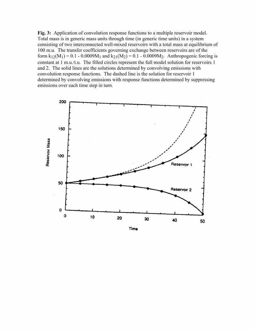
Fig. 3: Application of convolution response functions to a multiple reservoir model. Total mass is in generic mass units through time (in generic time units) in a system consisting of two interconnected well-mixed reservoirs with a total mass at equilibrium of 100 m.u. The transfer coefficients governing exchange between reservoirs are of the form k12(M1) = 0.1 - 0.0009M1 and k21(M2) = 0.1 - 0.0009M2. Anthropogenic forcing is constant at 1 m.u./t.u. The filled circles represent the full model solution for reservoirs 1 and 2. The solid lines are the solutions determined by convolving emissions with convolution response functions. The dashed line is the solution for reservoir 1 determined by convolving emissions with response functions determined by suppressing emissions over each time step in turn.

Fig. 4A: Transfer coefficient as a function of donor reservoir size for photosynthetic reservoirs for two emissions scenarios. The parameter k represents the fraction of atmospheric carbon content transferred to either photosynthetic reservoir per unit time. Convolution response functions are calculated assuming k is a linear function of atmospheric carbon; the figure shows this is approximately true, especially for low atmospheric CO2 concentrations.

Fig. 4B: Transfer coefficient as a function of donor reservoir size for the oceanic mixed layer for two emissions scenarios. The parameter k represents the fraction of mixed layer carbon content transferred to the atmosphere per unit time. Convolution response functions are calculated assuming k is a linear function of mixed layer carbon; the figure shows this is approximately true, especially for low carbon contents.

Fig. 5: (A) Fossil fuel emissions scenarios based on IS92a and IS92c scenarios and extended beyond 2100. (B) Atmospheric concentrations resulting from IS92a and IS92c scenarios.

Fig. 6: Convolution and impulse response functions for emissions in 1990 according to the IS92a and IS92c scenarios.

Fig. 7: Convolution and impulse response functions converted to impact on radiative forcing for emissions in 1990 according to the IS92a and IS92c scenarios. Forcing is measured relative to the initial change in radiative forcing in 1990.

Fig. 8: Integrated radiative forcing due to emission of an extra ton of CO2 in 1990 calculated for two emissions scenarios using both convolution and impulse response functions. After 500 years, convolution response functions indicate 20-30% less forcing than impulse response functions.

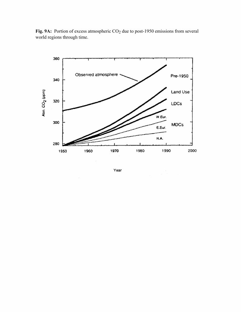
Fig. 9A: Portion of excess atmospheric CO2 due to post-1950 emissions from several world regions through time.

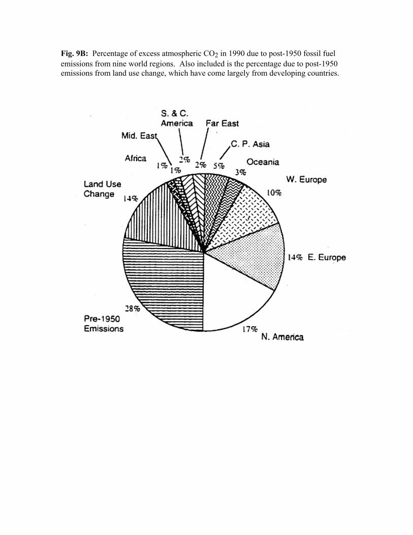
Fig. 9B: Percentage of excess atmospheric CO2 in 1990 due to post-1950 fossil fuel emissions from nine world regions. Also included is the percentage due to post-1950 emissions from land use change, which have come largely from developing countries.

Table 1: Marginal damage estimates in $/tC for three different response functions applied to emission in 1990.

Scenario Impulse Response, ocean-only model

Impulse Response, balanced model

Convolution Response

ρ = 0.0% IS92a $43 $48 $39 IS92c $36 $34 $31

ρ = 0.5% IS92a $30 $30 $26 IS92c $25 $23 $21

ρ = 3.0% IS92a $10 $9 $9 IS92c $9 $8 $8

Table 2: Marginal damages in $/tC for three different response functions applied to emissions at three different times.

Scenario Impulse Response, ocean-only model

Impulse Response, balanced model

Convolution Response

IS92a 1990 $30 $30 $26 2020 $43 $46 $41 2050 $53 $62 $53

IS92c 1990 $25 $23 $21 2020 $27 $26 $24 2050 $27 $27 $25