Measuring Retention in a Baby Diaper

Method development for baby diaper testing: From testing principal

to an optimized and evaluated method

Bachelor of Science Thesis in Chemical Engineering

HENRIK HAMMARSTRAND

Project performed at SCA Hygiene Products, Gothenburg

Department of chemical and biological engineering

CHALMERS UNIVERSITY OF TECHNOLOGY

Gothenburg, Sweden, 2013

Contents 1. Introduction ......................................................................................................................................... 1

2. Background .......................................................................................................................................... 1

3. Theory .................................................................................................................................................. 3

4. Methodology ....................................................................................................................................... 8

5. Results and discussion ....................................................................................................................... 13

6. Conclusion ......................................................................................................................................... 26

7. Recommendation .............................................................................................................................. 27

8. References ......................................................................................................................................... 28

Appendix 1: The DOE optimization test ................................................................................................ 30

Appendix 2: The verification test .......................................................................................................... 33

Appendix 3: Result Interpretation ......................................................................................................... 38

Appendix 4: X ray images ...................................................................................................................... 39

Appendix 5: Additional equations ......................................................................................................... 41

List of figures

Figure 1: The four layers of a baby diaper and the liquid spread direction p.3 Figure 2: Length wise cross section principal sketch of Product Y p.4 Figure 3: Length wise cross section principal sketch of Product B p.4 Figure 4: Length wise cross section principal sketch of Product C p.5 Figure 5: Illustration of liquid flow in one capillaries, due to the p.5 intermolecular attraction between the liquid and the walls of the capillary Figure 6: The degrees of freedom in an absorbent polymer p.6 Figure 7: Flow chart of the testing procedure p.8 Figure 8: Flow chart of method development procedure p.10 Figure 9: Weight values as a response of time for the first equipment set up p.14 Figure 10: The result graphs for the different times of constant pressure p.15 Figure 11: Illustration of the magnitude of the 20 test series, center points for product Y marked with red and for product B with green. p.17 Figure 12: Pareto chart of effects for average firstP p.17 Figure 13: Pareto chart of effects for stdev. firstP p.18 Figure 14: Pareto chart of effects for average totW p.18 Figure 15: Pareto chart of effects for stdev. totW. P.18 Figure 16: Pareto chart of effects for Rel.int p.19 Figure 17 The results for all (+) samples and all (-) samples, product B as response of time for run 13-20 in the DOE. The green lines represent the actual pressure. P.21 Figure 18: The results for all (+) samples and all (-) samples, product Y p.21 Figure 19: The results for all (+) samples and all (-) samples, product Y p.22 Figure 20: Individual value plot showing the difference between (+) and (-) regarding firstP p.23 Figure 21: Individual value plot showing the difference

between (+) and (-) regarding totW p.23 Figure 22: A (+) product B to the left, a (-) product B to the right p.24 Figure 23: Collection of graphs showing weight of liquid(blue line) as response of time for run 1-12 in the DOE. P.30 The green lines represent the actual pressure Figure 24: Collection of graphs showing weight of liquid(blue line) as response of time for run 13-20 in the DOE. The green lines represent the actual pressure p.31 Figure 25: Visualization of the Int. calculations for sample 3 in the DOE p.37 Figure 26: example of a b- sample p.38 Figure 27: example of a b+ sample p.38 Figure28: Example of c- sample p.38 Figure29: Example of c+ sample p.38 Figure 30: Example of a y- sample p.39 Figure 31: Example of a y+ sample p.39

List of tables

Table 1: Run order for the verification test, where (+) means more absorption p.12

material in the pressure area, and (-) means less

Table 2: Results from testing the vacuum pressure. Lowp=-0,2 bar, highp=-0,38 bar p.15

Table3: Summary of how the parameters should be optimized according to the DOE.

Brackets mean either it has a synergy effect of the p-value is above 0,05 p.19

Table 4: The optimal combination of parameters for the method p.19

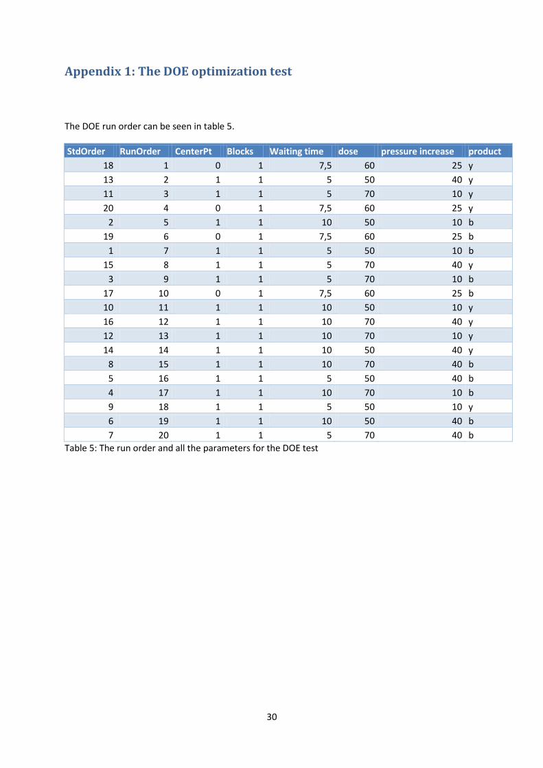
Table 5: The run order and all the parameters for the DOE test p.29

Table 6: All parameters included in the models, on all the different results for the p.32

DOE optimization

Table 7: Descriptive statistics of the verification test results p.33

List of equations

Equation 1: The Washburn expression p.5

Equation 2: Swelling based on Fick´s second law of diffusion p.6

Equation 3: The ideal gas law p.7

Equation 4: Calculation of Int for one sample p.37

Equation 5: Calculation of Rel.int for one sample p.37

Equation 6: Bernoullis equation for an ideal system p.40

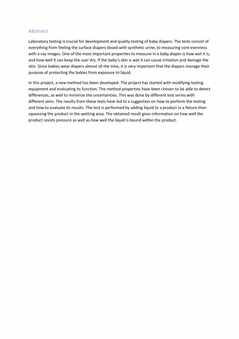
Abstract

Laboratory testing is crucial for development and quality testing of baby diapers. The tests consist of

everything from feeling the surface diapers dosed with synthetic urine, to measuring core evenness

with x-ray images. One of the most important properties to measure in a baby diaper is how wet it is,

and how well it can keep the user dry. If the baby’s skin is wet it can cause irritation and damage the

skin. Since babies wear diapers almost all the time, it is very important that the diapers manage their

purpose of protecting the babies from exposure to liquid.

In this project, a new method has been developed. The project has started with modifying testing

equipment and evaluating its function. The method properties have been chosen to be able to detect

differences, as well to minimize the uncertainties. This was done by different test series with

different aims. The results from these tests have led to a suggestion on how to perform the testing

and how to evaluate its results. The test is performed by adding liquid to a product in a fixture then

squeezing the product in the wetting area. The obtained result gives information on how well the

product resists pressure as well as how well the liquid is bound within the product.

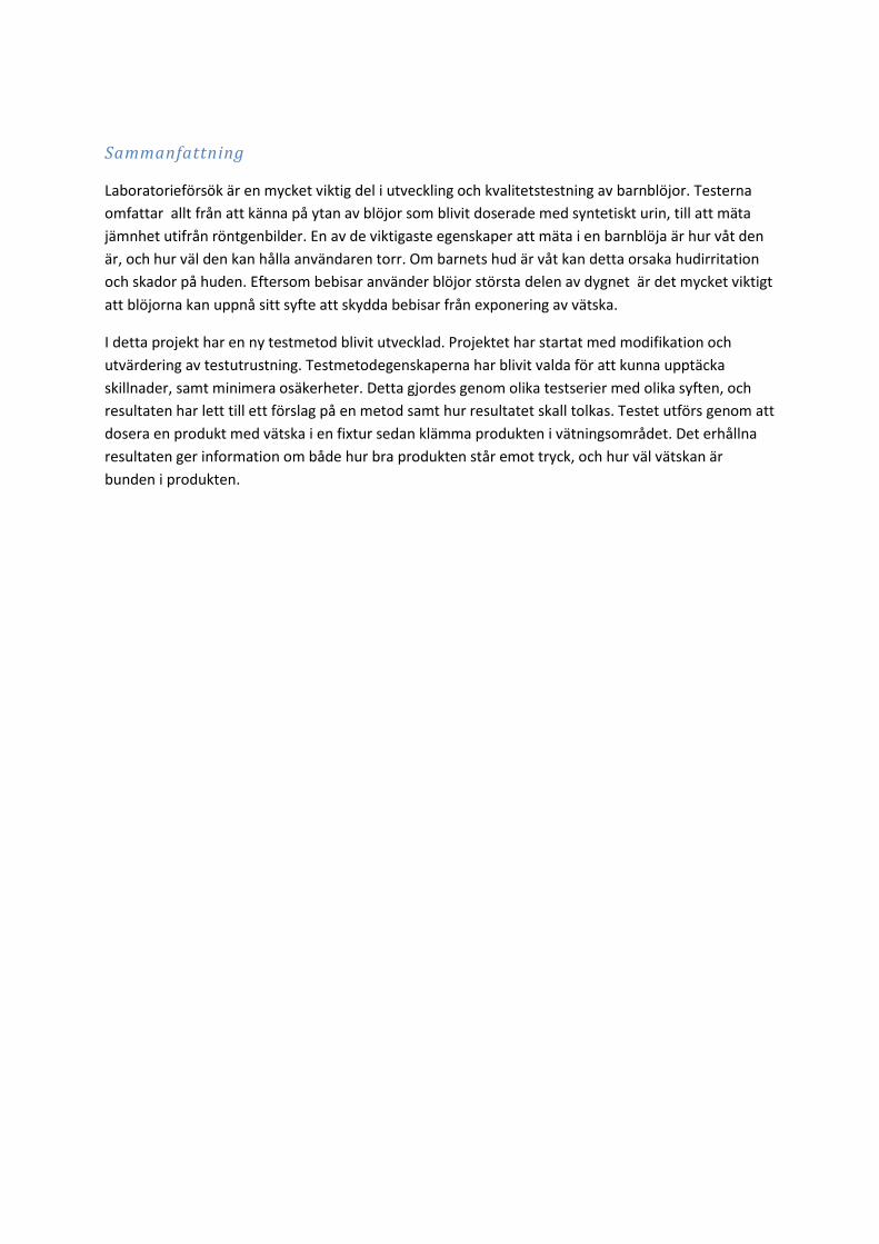
Sammanfattning

Laboratorieförsök är en mycket viktig del i utveckling och kvalitetstestning av barnblöjor. Testerna

omfattar allt från att känna på ytan av blöjor som blivit doserade med syntetiskt urin, till att mäta

jämnhet utifrån röntgenbilder. En av de viktigaste egenskaper att mäta i en barnblöja är hur våt den

är, och hur väl den kan hålla användaren torr. Om barnets hud är våt kan detta orsaka hudirritation

och skador på huden. Eftersom bebisar använder blöjor största delen av dygnet är det mycket viktigt

att blöjorna kan uppnå sitt syfte att skydda bebisar från exponering av vätska.

I detta projekt har en ny testmetod blivit utvecklad. Projektet har startat med modifikation och

utvärdering av testutrustning. Testmetodegenskaperna har blivit valda för att kunna upptäcka

skillnader, samt minimera osäkerheter. Detta gjordes genom olika testserier med olika syften, och

resultaten har lett till ett förslag på en metod samt hur resultatet skall tolkas. Testet utförs genom att

dosera en produkt med vätska i en fixtur sedan klämma produkten i vätningsområdet. Det erhållna

resultaten ger information om både hur bra produkten står emot tryck, och hur väl vätskan är

bunden i produkten.

Acknowledgments

I will start by thanking my supervisor Rozalia Bitis, for invaluable support and knowledge. You have

truly guided my path and this would not have been possible without you.

Special thanks to my examiner Ulf Jäglid for providing your scientific knowledge and helping me with

the project.

My gratitude to the Technical Laboratory support group TLS for lending me your expertise.

Thanks to my friend Anton Persson for a small yet valuable favor.

Lots of gratitude to SCA for the founding, and thanks all the employees at Baby Laboratory.

1

1. Introduction 1.1 aim

The aim of this study is to develop a stable and reliable measurement system i.e. test equipment and

test method, for measurement of rewet properties in baby diapers. A new analysis principal will be

tested, namely gradient pressure. The uncertainty of the measurement system should be low enough

to allow proper statistical evaluation of data. This study will focus on the process of developing an

operational and evaluated analysis method for laboratory tests.

1.2 purpose

Baby laboratory has need of a new and more reliable method for measuring retention than the

methods available today. Several different methods have been used to measure retention, but none

of these methods have the ability to compare retention in thin diapers that correlate to real use.

Product development of baby diapers has led to thinner diapers, and either the measurement

systems have to be adopted to handle thin products, or new methods have to be developed.

1.3 Demarcation

This project will strive towards the mentioned aim, but the timeframe of 10 weeks will set the

boundaries for the project.

One factorial design matrix will be performed and one measurement system evaluation. The project

will not include any new equipment, but the needed system development and equipment

optimization will be performed with the aid of the Technical laboratory support group (TLS). Three

predefined products will be used as test samples, and no new products will be tested.

2. Background 2.1 SCA

SCA is northern Europe´s largest forest company[1]. Its business consists of three branches, personal

care products, forest products and tissue products, and the company conducts sales in roughly 100

countries[1]. The gross revenue year 2011 surpassed 80 billion SEK, which makes it one of the largest

companies in Sweden[1][2]. The company started in 1927 as a merger of several smaller forest and

milling companies[1], and has vigorously grown ever since. The branch of interest for this study is the

personal care branch, and the rest of this article will primarily treat that part of the company.

Personal care accounted for 30% of SCA´s revenue the year 2012[3] and has many world renown

brands such as Tena, Libro and Libresse. The Personal care branch of SCA is divided into baby hygiene

products, incontinence products, and feminine hygiene products where each division has large

amounts of sales worldwide[3][1]. The Personal care part of the company started out in 1975 when

SCA bought Mölnlycke health care, thereby gaining access to all of Mölnlyckes brands, e.g. Libero and

Libresse[1]. The single largest category of health care products is incontinence care, which accounts

for roughly 50% of sales. Second largest in terms of sales is baby care products, which accounts for

2

close to 30%. This study is performed on the account of baby laboratory, but the results may influent

the other research and development departments as well.

2.2 The modern disposable diaper

Disposable diapers have been available since the 1940s[4] and account the major part of sales in

today’s baby hygiene market. Continuous development has led to the very efficient diapers that are

available today. The production companies are constantly working on achieving sustainable products

capable of meeting the market’s demands.

Three parameters are often discussed when investigating the performance of a diaper: Inlet time,

surface dryness and retention capacity. Inlet time is the time it takes for liquid to be absorbed into

the product. Failure to rapidly absorb liquid could disrupt the comfort and in worst case lead to

leakage. Retention is a measurement of how well the core can retain the absorbed liquid. Failure to

keep the absorbed liquid in the core can lead to wet skin for the user. Surface dryness is a

measurement of how wet the material in contact with the user’s skin is and how much liquid can be

extracted from that material. If the surface material is wet, this will affect the user regardless of how

well retention and inlet time work. All these measurement parameters intend to give information on

how well a product can keep babies dry. Failure in any of these three measurements is enough to

require improvement, and so all three have to be thoroughly investigated.

It is important to keep in mind that these three parameters are in direct conflict with each other.

Inlet time is shortened by using a more hydrophilic surface material, but that would make it harder to

drain the surface material, and to keep liquid from coming back up i.e. worse surface dryness and

retention. The reality for baby care products is always a compromise, forcing the products to be

optimized with all kinds of properties.

2.3The skin barrier

Skin is one of the most important barriers for a human being[5], and serves to protect us from many

hazards. Human skin mainly consists of three different types of polar lipids namely ceramides,

cholesterols and free fatty acids[5]. Since humans have very narrow acceptance limits for electrolyte

concentration in body fluids, the skin has to precisely control which substances are allowed to pass[5].

The skin is rather impermeable to water, but if water of high ion concentration is in contact with the

skin, there will be an osmotic pressure forcing water out of the skin[5]. A liquid with the ion

concentration similar to urine causes a relatively high pressure, and exposure to such a liquid can

disrupt the balance and cause skin irritation[5][6]. It has been documented that exposure to urine has

significant effect on skin irritation [6], thus it is very important to protect the body from long periods

of exposure.

3

3. Theory 3.1 The products

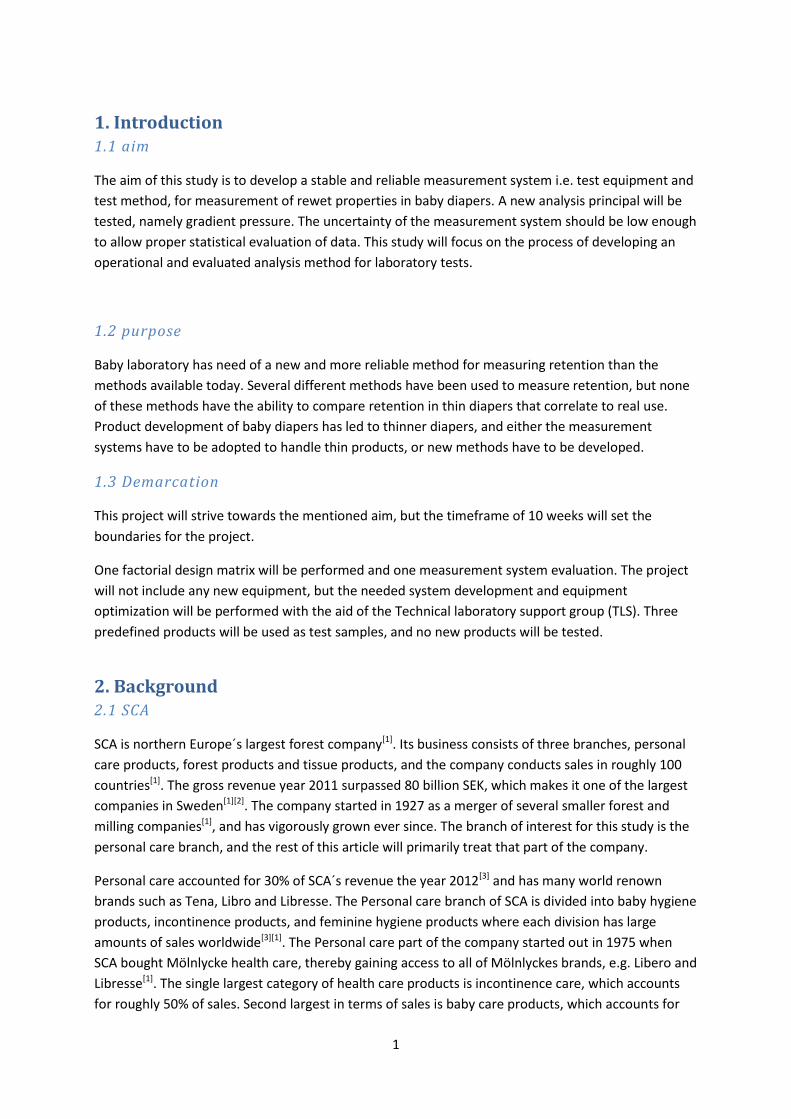
The baby diapers in this project consist of four layers as shown in figure 1. Only a brief explanation of

all the parts will be given in this report, for more information see reference 4.

Figure 1: The four layers of a baby diaper and the liquid spread direction.

The first part of the diaper is the layer in contact with the skin. This is called a top sheet and is

typically made of hydrophilic nonwoven materials. The reason why the top sheet is hydrophilic is to

enable fast absorption of all liquid that is in contact with the wearer’s skin, and to keep the skin

dry[4][5][6]. The second part is called a distribution layer. This layer is what drains the top sheet of

moisture[7]. The distribution layer also disperses all the liquid from the top sheet as much as possible,

to increase the contact area of the absorption core, and keep the core from getting locally

saturated[4]. The distribution layer in the three tested product has been made of two layers of

hydrophilic nonwoven and fiber between them. When the product is subjected to external pressure

between the top sheet and the absorption core, the distribution material should work as a

protection. A distribution layer with good mechanical properties prevents liquid from easily traveling

through. This protects the user from retention[7]. The third layer is the absorption core, made of SAP

(super absorbent polymer) and pulp[7].

Pulp has excellent absorption properties with strong capillary forces able to absorb and transport

liquid, even counter gravitationally[8][9][10]. Pulp has high absorption capacity per weight and fast

absorption rate, but the drawback is that it cannot sustain liquid under pressure, see section [3.2] for

absorption mechanics. To increase absorption capacity further and to improve retention properties,

there is often SAP in the diapers as well.

SAP is less expensive than pulp[11][12][13] and can absorb tremendous amounts of pure water, up to

1000g liquid/g SAP[8][9]. It has the ability to sustain liquid under pressure[12]. The drawback with SAP is

that is absorbs liquid much slower than pulp, for absorption mechanism see section [3.3]. SAP in

combination with pulp is what most baby diaper cores consist of today[7]. The two materials in

harmony can provide an absorption core with fast absorption, good distribution, extreme absorption

capacity and the ability to withstand pressure.

4

3.1.1 Test product Y, size 4 (7-14 kg):

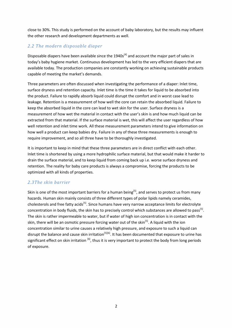
The Product Y is displayed in figure 2. It contains: A top sheet made of a hydrophilic nonwoven

material, a distribution layer of similar thickness to product C (section 3.2.3). It has two cores, and a

back sheet made of an impermeable, hydrophobic polymer material.

The cores consist of pulp and SAP. There are drainage channels in the core, spaces with no

absorption material, for good fit and eased transportation of liquid. The product has two cores to

focus the absorption to the front of the product. The first core covers the whole product, and the

second part is smaller and focused to the most likely wetting area. At the bottom and the top of the

core, are covering layers of only pulp and no SAP, to prevent SAP penetration to the product surface.

The core is kept in place with a core wrap.

- Hydrophilic top sheet

- Distribution layer

- The top of the core wrap

- Two cores of mixed SAP and pulp, a small and a large

- The bottom of the core wrap

- Hydrophobic back sheet

Figure 2: Length wise cross section principal sketch of Product Y.

3.1.2 Test product B, size 4(7-18 kg):

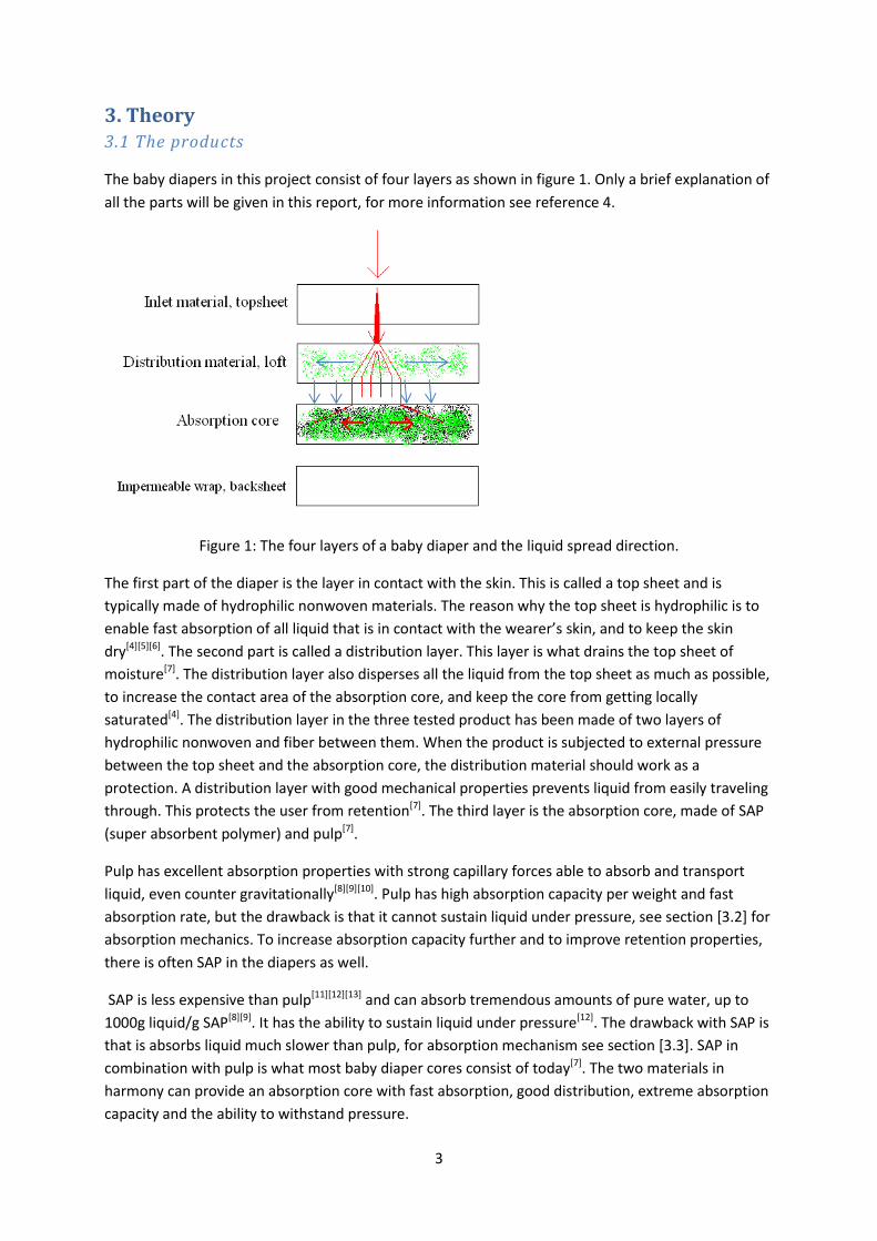
Product B (figure 3) contains: A top sheet of a hydrophilic nonwoven material. It has a thicker loft

than product Y and C. The core is a laminate of two nonwoven materials with SAP between them.

Product B has a core wrap glued to the loft as well as the back sheet, surrounding the core. The core

is made of only SAP and no pulp. The top and the bottom of the core are glued in a pattern of

squares that trap the SAP. When enough liquid has been absorbed, the squares burst due to the

swelling of the SAP

- Hydrophilic top sheet

- Distribution layer

- Top nonwoven of the laminate

- Encapsulated SAP particles

- Bottom nonwoven of the laminate

- Hydrophobic back sheet

Figure 3: Length wise cross section principal sketch of Product B.

3.1.3 Test product C, size 4(7-18 kg)

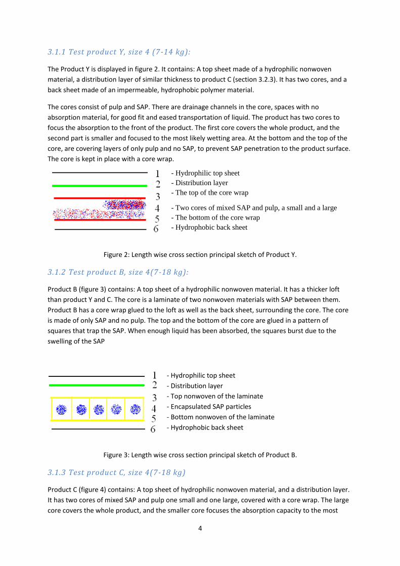
Product C (figure 4) contains: A top sheet of hydrophilic nonwoven material, and a distribution layer.

It has two cores of mixed SAP and pulp one small and one large, covered with a core wrap. The large

core covers the whole product, and the smaller core focuses the absorption capacity to the most

5

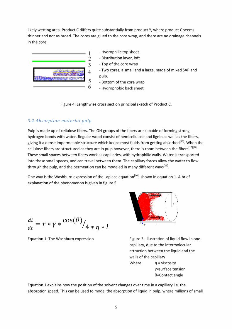
likely wetting area. Product C differs quite substantially from product Y, where product C seems

thinner and not as broad. The cores are glued to the core wrap, and there are no drainage channels

in the core.

- Hydrophilic top sheet

- Distribution layer, loft

- Top of the core wrap

- Two cores, a small and a large, made of mixed SAP and

pulp.

- Bottom of the core wrap

- Hydrophobic back sheet

Figure 4: Lengthwise cross section principal sketch of Product C.

3.2 Absorption material pulp

Pulp is made up of cellulose fibers. The OH groups of the fibers are capable of forming strong

hydrogen bonds with water. Regular wood consist of hemicellulose and lignin as well as the fibers,

giving it a dense impermeable structure which keeps most fluids from getting absorbed[10]. When the

cellulose fibers are structured as they are in pulp however, there is room between the fibers[10][16].

These small spaces between fibers work as capillaries, with hydrophilic walls. Water is transported

into these small spaces, and can travel between them. The capillary forces allow the water to flow

through the pulp, and the permeation can be modeled in many different ways[15].

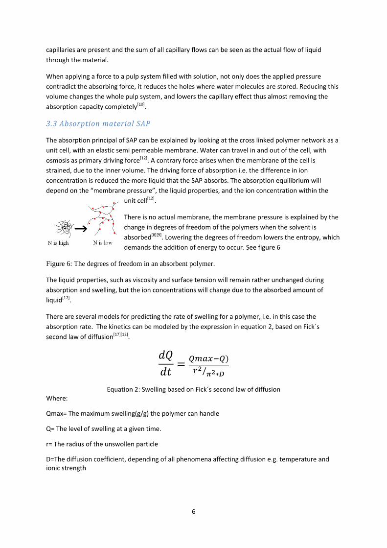
One way is the Washburn expression of the Laplace equation[10], shown in equation 1. A brief

explanation of the phenomenon is given in figure 5.

⁄

Equation 1: The Washburn expression Figure 5: Illustration of liquid flow in one

capillary, due to the intermolecular

attraction between the liquid and the

walls of the capillary

Where: η = viscosity

γ=surface tension

θ=Contact angle

Equation 1 explains how the position of the solvent changes over time in a capillary i.e. the

absorption speed. This can be used to model the absorption of liquid in pulp, where millions of small

6

capillaries are present and the sum of all capillary flows can be seen as the actual flow of liquid

through the material.

When applying a force to a pulp system filled with solution, not only does the applied pressure

contradict the absorbing force, it reduces the holes where water molecules are stored. Reducing this

volume changes the whole pulp system, and lowers the capillary effect thus almost removing the

absorption capacity completely[10].

3.3 Absorption material SAP

The absorption principal of SAP can be explained by looking at the cross linked polymer network as a

unit cell, with an elastic semi permeable membrane. Water can travel in and out of the cell, with

osmosis as primary driving force[12]. A contrary force arises when the membrane of the cell is

strained, due to the inner volume. The driving force of absorption i.e. the difference in ion

concentration is reduced the more liquid that the SAP absorbs. The absorption equilibrium will

depend on the “membrane pressure”, the liquid properties, and the ion concentration within the

unit cell[12].

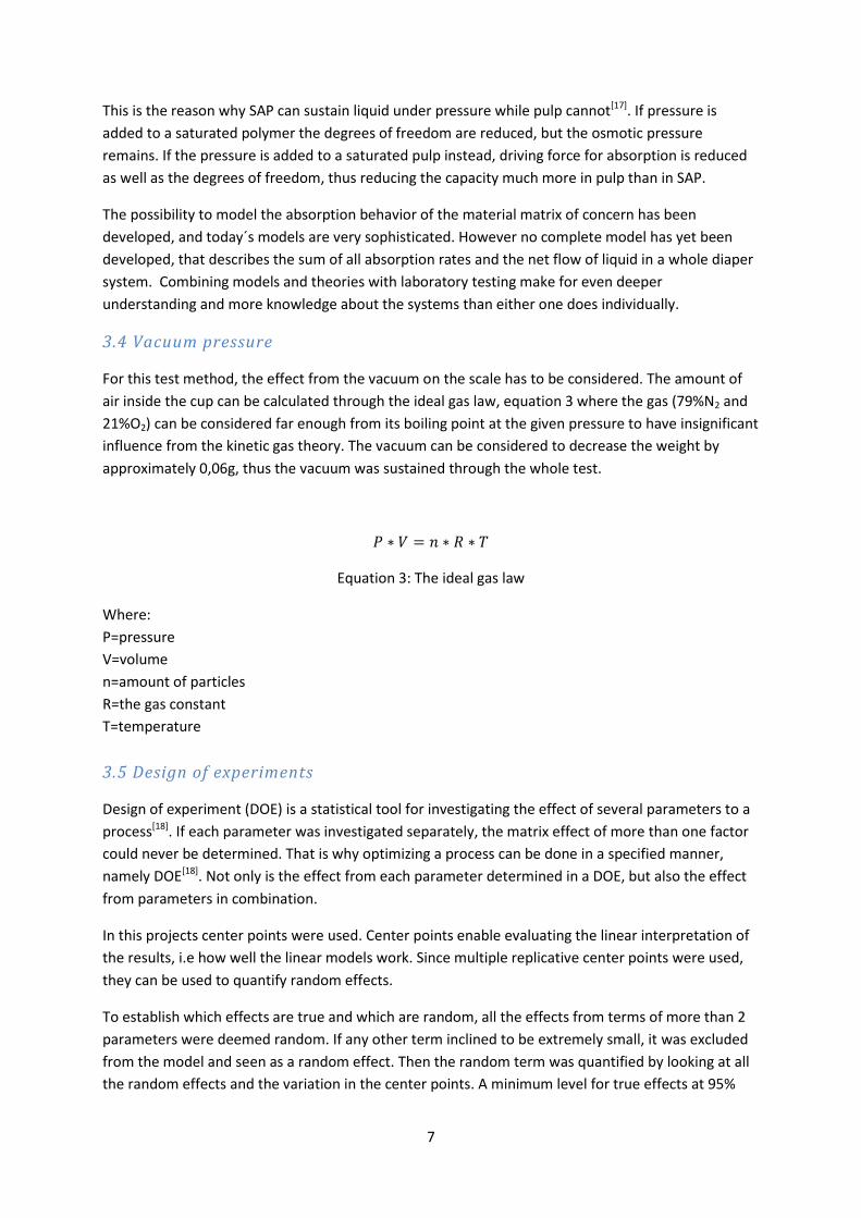
There is no actual membrane, the membrane pressure is explained by the

change in degrees of freedom of the polymers when the solvent is

absorbed[8][9]. Lowering the degrees of freedom lowers the entropy, which

demands the addition of energy to occur. See figure 6

Figure 6: The degrees of freedom in an absorbent polymer.

The liquid properties, such as viscosity and surface tension will remain rather unchanged during

absorption and swelling, but the ion concentrations will change due to the absorbed amount of

liquid[17].

There are several models for predicting the rate of swelling for a polymer, i.e. in this case the

absorption rate. The kinetics can be modeled by the expression in equation 2, based on Fick´s

second law of diffusion[17][12].

Equation 2: Swelling based on Fick´s second law of diffusion Where:

Qmax= The maximum swelling(g/g) the polymer can handle

Q= The level of swelling at a given time.

r= The radius of the unswollen particle

D=The diffusion coefficient, depending of all phenomena affecting diffusion e.g. temperature and ionic strength

7

This is the reason why SAP can sustain liquid under pressure while pulp cannot[17]. If pressure is

added to a saturated polymer the degrees of freedom are reduced, but the osmotic pressure

remains. If the pressure is added to a saturated pulp instead, driving force for absorption is reduced

as well as the degrees of freedom, thus reducing the capacity much more in pulp than in SAP.

The possibility to model the absorption behavior of the material matrix of concern has been

developed, and today´s models are very sophisticated. However no complete model has yet been

developed, that describes the sum of all absorption rates and the net flow of liquid in a whole diaper

system. Combining models and theories with laboratory testing make for even deeper

understanding and more knowledge about the systems than either one does individually.

3.4 Vacuum pressure

For this test method, the effect from the vacuum on the scale has to be considered. The amount of

air inside the cup can be calculated through the ideal gas law, equation 3 where the gas (79%N2 and

21%O2) can be considered far enough from its boiling point at the given pressure to have insignificant

influence from the kinetic gas theory. The vacuum can be considered to decrease the weight by

approximately 0,06g, thus the vacuum was sustained through the whole test.

Equation 3: The ideal gas law

Where:

P=pressure

V=volume

n=amount of particles

R=the gas constant

T=temperature

3.5 Design of experiments

Design of experiment (DOE) is a statistical tool for investigating the effect of several parameters to a

process[18]. If each parameter was investigated separately, the matrix effect of more than one factor

could never be determined. That is why optimizing a process can be done in a specified manner,

namely DOE[18]. Not only is the effect from each parameter determined in a DOE, but also the effect

from parameters in combination.

In this projects center points were used. Center points enable evaluating the linear interpretation of

the results, i.e how well the linear models work. Since multiple replicative center points were used,

they can be used to quantify random effects.

To establish which effects are true and which are random, all the effects from terms of more than 2

parameters were deemed random. If any other term inclined to be extremely small, it was excluded

from the model and seen as a random effect. Then the random term was quantified by looking at all

the random effects and the variation in the center points. A minimum level for true effects at 95%

8

confidence level is used in this project, and the effects have to surpass this level to be considered

true. DOE is a commonly used statistical tool at SCA Gothenburg[9][19].

4. Methodology

4.1Test setup

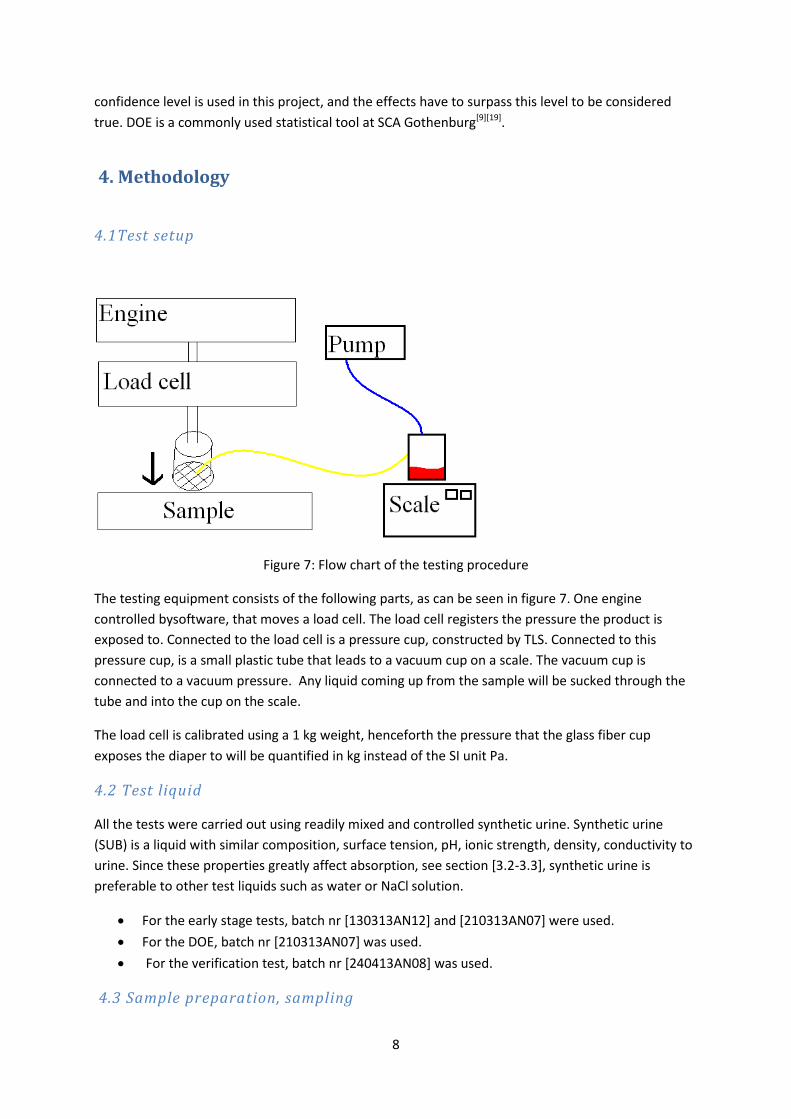
Figure 7: Flow chart of the testing procedure

The testing equipment consists of the following parts, as can be seen in figure 7. One engine

controlled bysoftware, that moves a load cell. The load cell registers the pressure the product is

exposed to. Connected to the load cell is a pressure cup, constructed by TLS. Connected to this

pressure cup, is a small plastic tube that leads to a vacuum cup on a scale. The vacuum cup is

connected to a vacuum pressure. Any liquid coming up from the sample will be sucked through the

tube and into the cup on the scale.

The load cell is calibrated using a 1 kg weight, henceforth the pressure that the glass fiber cup

exposes the diaper to will be quantified in kg instead of the SI unit Pa.

4.2 Test liquid

All the tests were carried out using readily mixed and controlled synthetic urine. Synthetic urine

(SUB) is a liquid with similar composition, surface tension, pH, ionic strength, density, conductivity to

urine. Since these properties greatly affect absorption, see section [3.2-3.3], synthetic urine is

preferable to other test liquids such as water or NaCl solution.

For the early stage tests, batch nr [130313AN12] and [210313AN07] were used.

For the DOE, batch nr [210313AN07] was used.

For the verification test, batch nr [240413AN08] was used.

4.3 Sample preparation, sampling

9

For all products used in the DOE and the verification test, the following procedure was followed:

200 products from the same manufacturing batch of each type were weighed one by one. The 120

products closest to the average weight were chosen for the testing, the rest were discarded. The

products were mixed and chosen at random for the DOE test series as well as the verification test

series. The dry weights were noted for each sample, and used as covariates for statistical tests in the

doe and the verification test.

All the chosen products were conditioned for 24 hours in a constant climate room of 23⁰C and 50%

air humidity.

The products for all the other tests were similar to product Y, though not from the same batch. They

were not weighed or conditioned. They were allowed to get decompressed inside minigrip bags for

at least one hour before testing.

4.4 Dosing

The samples were put up in a fairly user like position, using metal fixtures. Velcro (burdock) patches

in combination with clips held the products in place.

The addition of liquid was executed automatically. The dosing was performed using a dosing

equipment with the liquid flow 10ml/s for all samples. To add different volumes, the dosing time was

changed. The dosage equipment was calibrated before each run, with acceptance criteria of 2%.

The time after the last dose was measured with a quartz controlled timer.

4.5 Test procedure

After pre-determined time, a sample with complete dosing was put under the load cell according to

figure 7. The engine lowers the glass fiber cup with high speed until the pressure of the load cell

reaches a starting value. The program continuously reads 2 values of load per second, as well as 2

values of weight per second. The computer then regulates the speed of the engine to achieve a linear

pressure increase. When the maximum pressure is reached, the pressure is kept constant during a

period of time. After the time for constant pressure, the engine is reset to starting position and the

data collection stops.

The program saves the weight data, as well as the pressure data. Each value of liquid weight

corresponds to a specific time, and at that specific time, the pressure is also registered. The program

plots the liquid weight, the actual pressure and the target pressure as responses of time for each

sample. One of these plots can be seen in Appendix 1, figure 23. After one test, the sample is

disposed and the next sample can be tested.

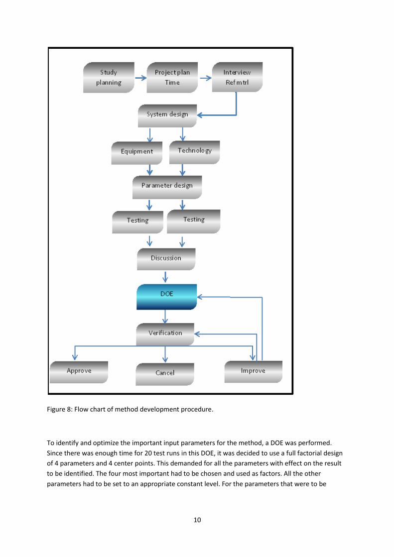
4.6 Method development procedure

Developing a test method from the very start required a well-structured procedure for setting up all

the tests and interpreting their result. This project aimed at following method development

procedure commonly used at SCA with regard to planning and execution. A brief description of the

main test series and their purposes is given in this section, for an overview see figure 8.

10

Figure 8: Flow chart of method development procedure.

To identify and optimize the important input parameters for the method, a DOE was performed.

Since there was enough time for 20 test runs in this DOE, it was decided to use a full factorial design

of 4 parameters and 4 center points. This demanded for all the parameters with effect on the result

to be identified. The four most important had to be chosen and used as factors. All the other

parameters had to be set to an appropriate constant level. For the parameters that were to be

11

factors in the DOE, suitable values for high and low level had to be found through testing and

discussion.

The test setup had to be evaluated, and the results from this can be seen in section [5.1]. After

concluding that the method could be run according to plan, and that the technical demands were

met, the vacuum pressure, the time for constant pressure, and the max pressure were tested to see

if they could be kept constant.

Then appropriate values for the high and the low levels of the factors in the DOE had to be found,

more about this in section [5.2.3]

The optimization test was run according to the schedule shown in appendix 1 table 5.

When the DOE was finished and the results interpreted, the outcomes together with a visual

evaluation were used to determine the final settings. A verification test was then performed, with

the three different products described in section [3.1]. The verification test was performed to analyze

how well the method performs regarding uncertainty and ability to detect differences between

products.

4.7 X-ray

Quantification of true uncertainty in the test method would require completely homogeny samples.

Since all manufacturing processes have some variation and because baby diapers are quite complex

material systems, this is practically impossible. For the possibility to analyze uncertainty regardless of

product unevenness, an attempt was made to connect core properties to test results.

To investigate the correlation between specific sample properties and results, products were

analyzed with x-ray images, which show the density of the core area. Since SAP has higher density

than pulp, a certain density would indicate a certain composition and distribution of SAP and pulp.

The products tested as center points in the DOE were chosen to be as similar as possible with regard

to distribution in the wetting area. For the verification test samples with much absorption material,

as well as samples with little absorption material were chosen.

X-ray images never show the whole picture, only the density of the core horizontally. Thus no

correlation to e.g. loft thickness or glue distribution can be investigated with this procedure. The x-

ray images do not either show how the absorption material is distributed vertically, whether the

material is close to the top sheet or the back sheet. However the images can be used to pick out

similar or very different products in means of SAP distribution.

In this work, the products tested as center points in the DOE were chosen to be as similar as possible

with regard to distribution in the wetting area. To collect more data on the effect that material

distribution has on the results, all the products in the verification test were analyzed in x-ray as well.

The results from these comparisons are discussed in section [5.4], examples of images can be seen in

appendix 4, figure 26-31

12

4.8 The verification test

After suggesting an optimal set of parameters for the testing procedure, a verification test was

performed. The test series was performed on the three products described in section [3.1] and 10

sample of each product was tested.

To understand the effects of the inhomogeneity of the core in the measuring area, all the products

were analyzed with x-ray. By visual evaluation of the images, 5 samples with high absorption

material density, and 5 samples with the contrary were chosen for each product type.

For the method to accurately handle many different types of products is absolutely crucial. There are

many types of products that will need to be tested, and this method should be able to analyze them

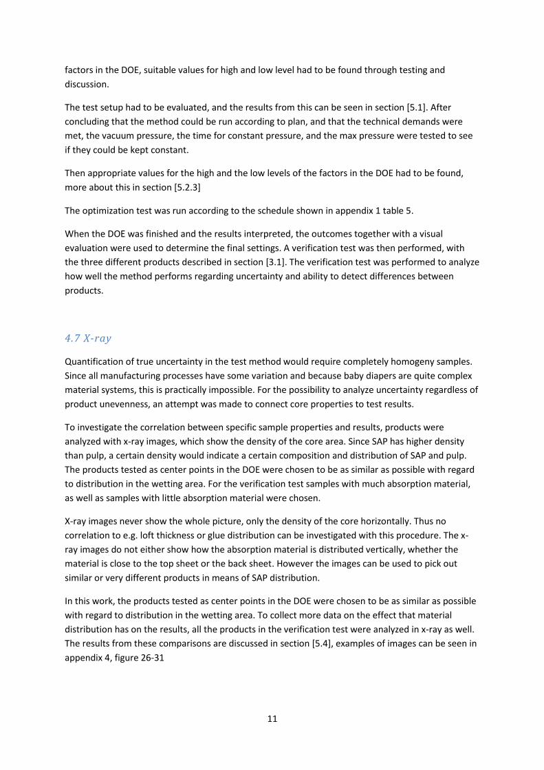
all, thus a third product is tested in this verification test. The tests are run in the order shown in

Table 1.

run order product absorption mrtl(+/-)

1 b -

2 b +

3 c +

4 c -

5 y -

6 y +

Table 1: Run order for the verification test, where (+) means more absorption material in the

pressure area, and (–) means less.

4.9 Analyzing the results

All statistical calculations were carried out using Minitab statistical software version 16. Simple

calculations were performed using Microsoft excel, and some graphs were made using Matlab.

Each sample gave approximately 200 data points, describing how liquid flows from the product under

pressure over a period of time. Having this amount of data poses the question of what is important

to analyze, from a development or an end user point of view. The two primary responses obtained

from the purposed method are:

-At which pressure does liquid start flowing out of the product? (firstP)

-How much liquid can be extracted from of the product? (totW)

These two responses provide important information on how products perform, both the aspect of

pressure resistance, and how well free liquid is retained. There are other possible ways of analyzing

the data, for example the flow rate at the start of the curve, or the decrease in flow rate over time

but firstP and totW were chosen for this project.

13

One of the most important aspects of the method is to have stable results, as can be seen in the aim

of the project. To achieve stability, the standard deviation (stdev.) was calculated for firstP as well as

totW, and both were used as responses in the DOE. Using these responses enabled optimization of

parameters to minimize the deviations in the method. The relative within group stdev. was used to

quantify repeatability in the verification test.

Another way of measuring uncertainty is to quantify the total area between the weight curves and

comparing them to the average of the weight curves. This way, not only the starting point or the end

point of the weight curves was analyzed. For more information about this method, see appendix 3

4.10 Information sources

To reach deeper understanding about the development division, two scientists at SCA were formally

interviewed, Ted Guidotti and Helena Corneliusson. Ted works as a senior scientist, and specializes in

absorption. The full protocol of the interview can be seen as reference 9. The second interviewed

employee is Helena Corneliusson, who is a lead product developer. Helena´s role is to assist

development projects with product expertize, and to take part in development projects. They both

have a great deal of experience of corporate development work, and take essential parts in lots of

different projects for baby hygiene product development. Helena´s interview is referred to as

reference 19.

The rest of the sources used were chosen by studying lots of scientific literature. All fields from

medical journals to fluid metrics were studied, and a few of the most reliable articles were chosen to

support the claims made in this article.

14

5. Results and discussion 5.1 System design

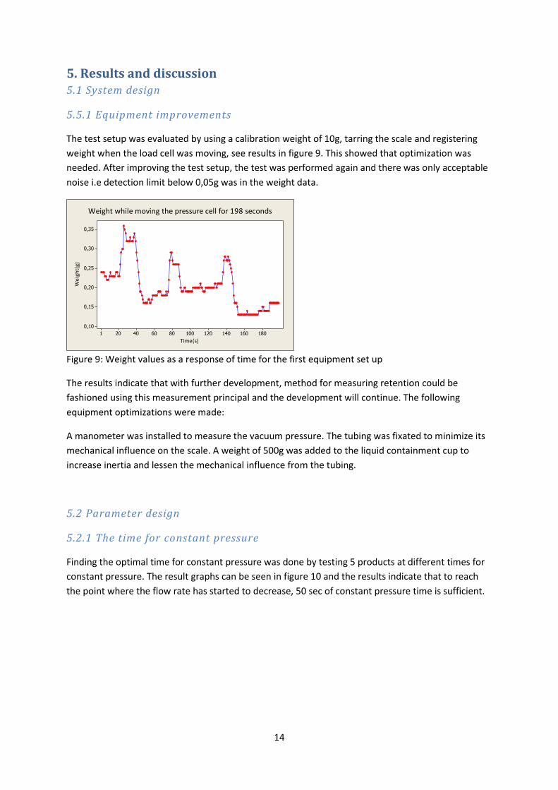
5.5.1 Equipment improvements

The test setup was evaluated by using a calibration weight of 10g, tarring the scale and registering

weight when the load cell was moving, see results in figure 9. This showed that optimization was

needed. After improving the test setup, the test was performed again and there was only acceptable

noise i.e detection limit below 0,05g was in the weight data.

180160140120100806040201

0,35

0,30

0,25

0,20

0,15

0,10

Time(s)

We

igh

t(g)

Weight while moving the pressure cell for 198 seconds

Figure 9: Weight values as a response of time for the first equipment set up

The results indicate that with further development, method for measuring retention could be

fashioned using this measurement principal and the development will continue. The following

equipment optimizations were made:

A manometer was installed to measure the vacuum pressure. The tubing was fixated to minimize its

mechanical influence on the scale. A weight of 500g was added to the liquid containment cup to

increase inertia and lessen the mechanical influence from the tubing.

5.2 Parameter design

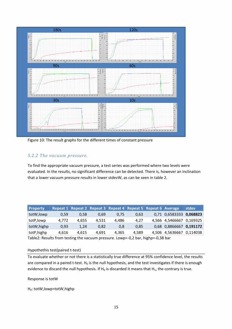
5.2.1 The time for constant pressure

Finding the optimal time for constant pressure was done by testing 5 products at different times for

constant pressure. The result graphs can be seen in figure 10 and the results indicate that to reach

the point where the flow rate has started to decrease, 50 sec of constant pressure time is sufficient.

15

180s 120s

90s 60s

30s 10s

Figure 10: The result graphs for the different times of constant pressure

5.2.2 The vacuum pressure.

To find the appropriate vacuum pressure, a test series was performed where two levels were

evaluated. In the results, no significant difference can be detected. There is, however an inclination

that a lower vacuum pressure results in lower stdevW, as can be seen in table 2.

Property Repeat 1 Repeat 2 Repeat 3 Repeat 4 Repeat 5 Repeat 6 Average stdev

totW,lowp 0,59 0,58 0,69 0,75 0,63 0,71 0,6583333 0,068823

totP,lowp 4,772 4,655 4,531 4,486 4,27 4,566 4,5466667 0,169325

totW,highp 0,93 1,24 0,82 0,8 0,85 0,68 0,8866667 0,191172

totP,highp 4,616 4,615 4,691 4,365 4,589 4,506 4,5636667 0,114038

Table2: Results from testing the vacuum pressure. Lowp=-0,2 bar, highp=-0,38 bar

Hypothethis test(paired t-test)

To evaluate whether or not there is a statistically true difference at 95% confidence level, the results

are compared in a paired t-test. H0 is the null hypothesis, and the test investigates if there is enough

evidence to discard the null hypothesis. If H0 is discarded it means that H1, the contrary is true.

Response is totW

H0: totW,lowp=totW,highp

16

H1: totW,lowp≠totW,highp

P=0,074, there is not enough evidence to say there is a true difference between the high level of

vacuum and the low level. It can be said that the p-value being as low as it is suggests that there may

be a difference, only is can’t be detected in this test.

This test resulted in the vacuum pressure not being evaluated in the DOE, and instead being set to

-0,2 Bar.

5.2.3 Choosing the DOE parameters

To decide an appropriate dose, data from several different projects was studied, discussion was held

and several company sources were consulted. The dose was then set to vary between 50 and 70 ml.

The product is dosed thrice, which means a total addition of liquid between 150 and 210 ml.

The waiting time between doses was set to a constant value while the waiting time after the last

dose varied. Due to the limitation of the equipment, the measurement can only be performed on one

sample at a time. This force the waiting time between doses to be balanced between time

consumption and sufficient time for the measurement itself. The time evaluation led to the waiting

time, between two doses, being set to 15 min and the waiting time after the last dose between 5 and

10 minutes.

To decide which max pressure and which slope of the pressure increase to use, careful consideration

had to be taken. There was not enough time to investigate both pressure increase time and max

pressure as separate parameters in the DOE. By evaluation of early tests as well as through

discussion, the time for pressure increase was varied between 10s and 40s. The pressure was then

chosen to be as low as possible, yet able to extract liquid in all parameter combinations. For this

purpose, the max pressure was set to 5 kg. Two center points for each product were used, for more

information about center points in a 2 level factorial DOE, see section [3.5]. Summarized, the

parameters in the DOE with high, low and center levels are summarized below:

product B - B&Y - Y

Waiting time 5 - 7,5 - 10

Dose 50 - 60 - 70

Pressure inc 10 - 25 - 40

5.2.4 The DOE results

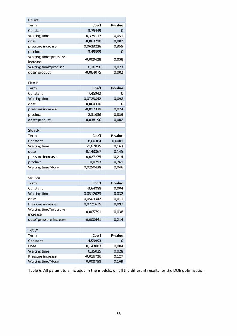
All the terms included in the models are displayed in Appendix 2 table 4 with their p-values and

coefficients. These were the guidelines for choosing optimal parameters. The stdev. values are

analyzed using the least square regression estimation method.

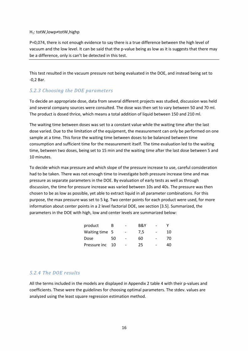
17

Figure 11: Illustration of the magnitude of the 20 test series, center points for product Y marked with

red and for product B with green.

As seen in figure 11 regarding Pstart, the center points show very similar results for both products.

For rewet (totW) on the other hand, the product B center points differ both in stdev. and totW. By

looking at the x-ray images of the products, this can be explained to some extent see section [5.7].

For totW, the product B was excluded from the model and the results analyzed based on only the

product Y part of the DOE.

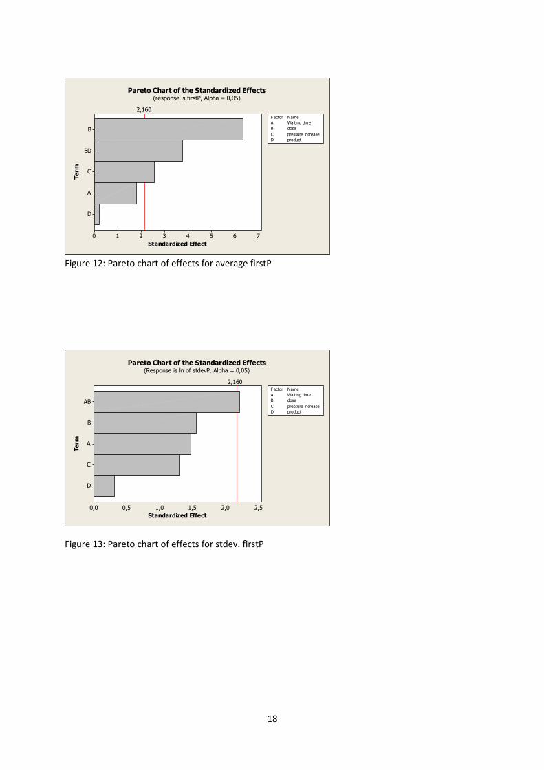
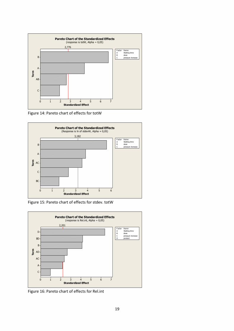
When the results of the DOE are analyzed, it has to be established which effects are true and which

are random. Pareto charts follow, in figure 12-16, which show all the effects from the factors in the

Doe result models. There is a red line in the Pareto charts, resembling the level that the effects have

to surpass to be considered true effects. All bars to the right of the red line are significant (true)

effects.

18

D

A

C

BD

B

76543210

Te

rm

Standardized Effect

2,160

A Waiting time

B dose

C pressure increase

D product

Factor Name

Pareto Chart of the Standardized Effects(response is firstP, Alpha = 0,05)

Figure 12: Pareto chart of effects for average firstP

D

C

A

B

AB

2,52,01,51,00,50,0

Te

rm

Standardized Effect

2,160

A Waiting time

B dose

C pressure increase

D product

F actor Name

Pareto Chart of the Standardized Effects(Response is ln of stdevP, Alpha = 0,05)

Figure 13: Pareto chart of effects for stdev. firstP

19

C

AB

A

B

76543210

Te

rm

Standardized Effect

2,776

A Waiting time

B dose

C pressure increase

Factor Name

Pareto Chart of the Standardized Effects(response is totW, Alpha = 0,05)

Figure 14: Pareto chart of effects for totW

BC

C

AC

A

B

6543210

Te

rm

Standardized Effect

3,182

A Waiting time

B dose

C pressure increase

Factor Name

Pareto Chart of the Standardized Effects(Response is ln of stdevW, Alpha = 0,05)

Figure 15: Pareto chart of effects for stdev. totW

C

A

AC

AD

B

BD

D

76543210

Te

rm

Standardized Effect

2,201

A Waiting time

B dose

C pressure increase

D product

Factor Name

Pareto Chart of the Standardized Effects(response is Rel.int, Alpha = 0,05)

Figure 16: Pareto chart of effects for Rel.int

20

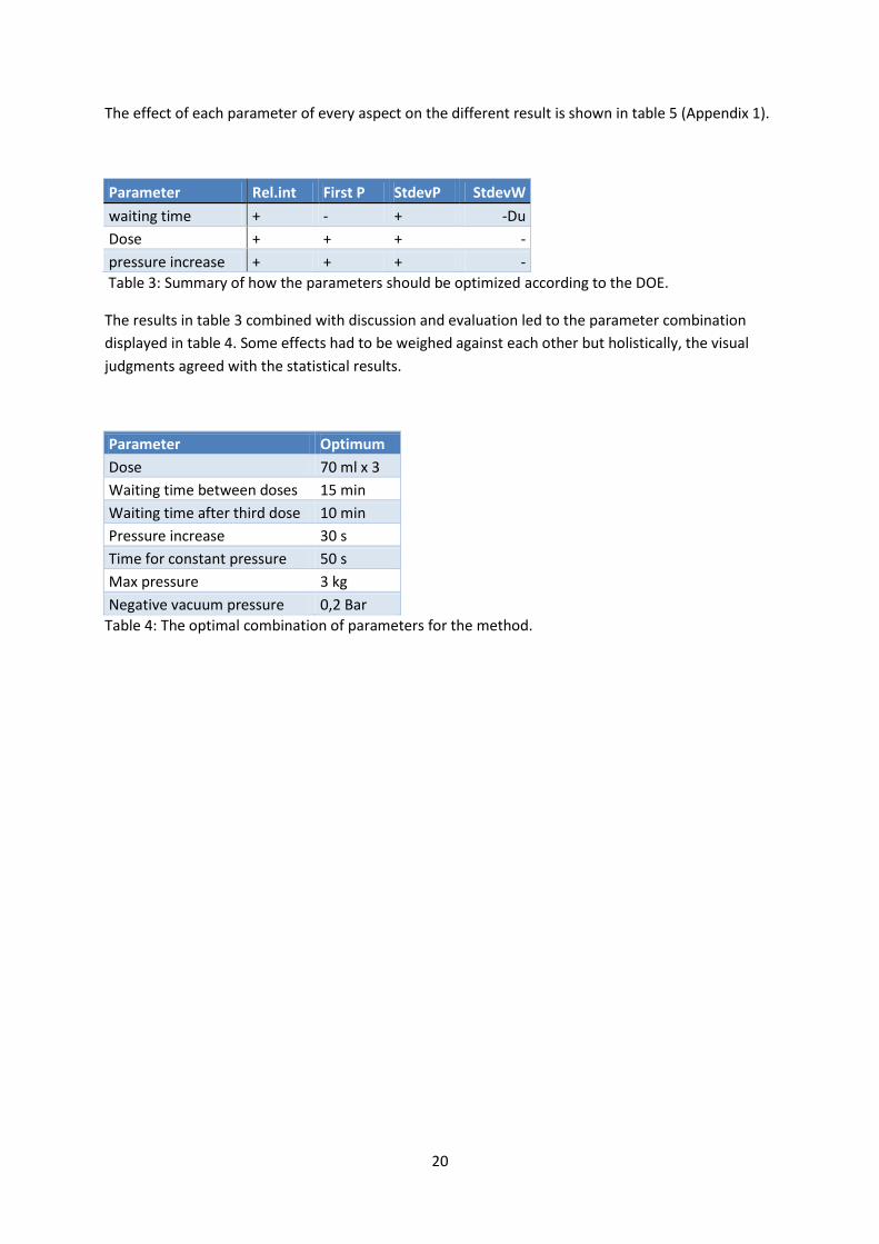
The effect of each parameter of every aspect on the different result is shown in table 5 (Appendix 1).

Parameter Rel.int First P StdevP StdevW

waiting time + - + -Du

Dose + + + -

pressure increase + + + -

Table 3: Summary of how the parameters should be optimized according to the DOE.

The results in table 3 combined with discussion and evaluation led to the parameter combination

displayed in table 4. Some effects had to be weighed against each other but holistically, the visual

judgments agreed with the statistical results.

Parameter Optimum

Dose 70 ml x 3

Waiting time between doses 15 min

Waiting time after third dose 10 min

Pressure increase 30 s

Time for constant pressure 50 s

Max pressure 3 kg

Negative vacuum pressure 0,2 Bar

Table 4: The optimal combination of parameters for the method.

21

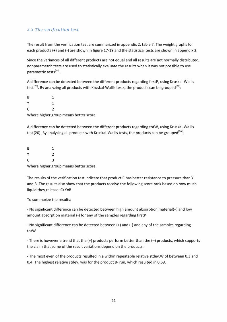
5.3 The verification test

The result from the verification test are summarized in appendix 2, table 7. The weight graphs for

each products (+) and (-) are shown in figure 17-19 and the statistical tests are shown in appendix 2.

Since the variances of all different products are not equal and all results are not normally distributed,

nonparametric tests are used to statistically evaluate the results when it was not possible to use

parametric tests[20].

A difference can be detected between the different products regarding firstP, using Kruskal-Wallis

test[20]. By analyzing all products with Kruskal-Wallis tests, the products can be grouped[20]:

B 1

Y 1

C 2

Where higher group means better score.

A difference can be detected between the different products regarding totW, using Kruskal-Wallis

test[20]. By analyzing all products with Kruskal-Wallis tests, the products can be grouped[20]:

B 1

Y 2

C 3

Where higher group means better score.

The results of the verification test indicate that product C has better resistance to pressure than Y

and B. The results also show that the products receive the following score rank based on how much

liquid they release: C>Y=B

To summarize the results:

- No significant difference can be detected between high amount absorption material(+) and low

amount absorption material (-) for any of the samples regarding firstP

- No significant difference can be detected between (+) and (-) and any of the samples regarding

totW

- There is however a trend that the (+) products perform better than the (–) products, which supports

the claim that some of the result variations depend on the products.

- The most even of the products resulted in a within repeatable relative stdev.W of between 0,3 and

0,4. The highest relative stdev. was for the product B- run, which resulted in 0,69.

22

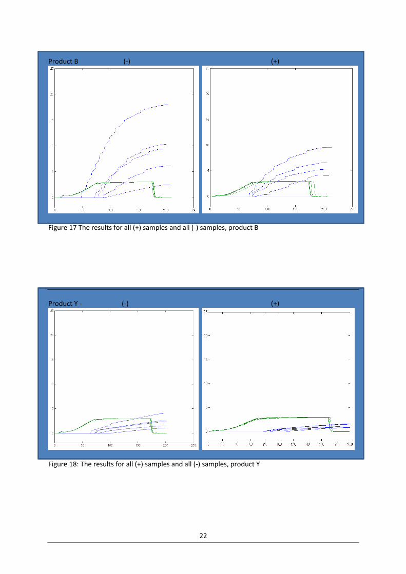
Product B (-) (+)

Figure 17 The results for all (+) samples and all (-) samples, product B

Product Y - (-) (+)

Figure 18: The results for all (+) samples and all (-) samples, product Y

23

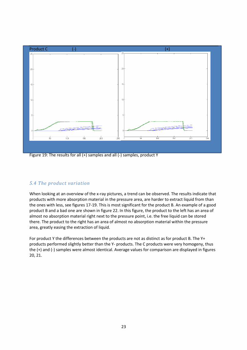
Product C (-) (+)

Figure 19: The results for all (+) samples and all (-) samples, product Y

5.4 The product variation

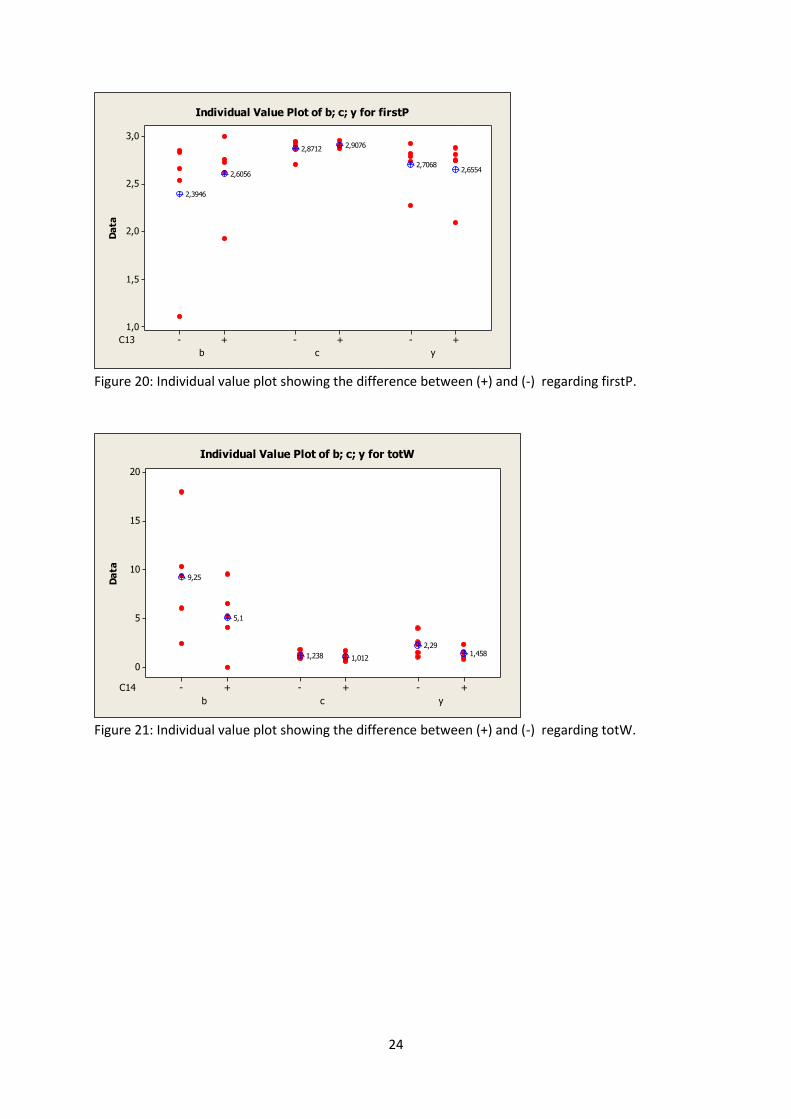
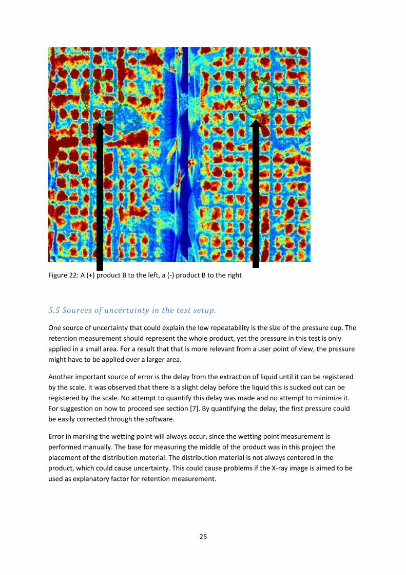
When looking at an overview of the x-ray pictures, a trend can be observed. The results indicate that products with more absorption material in the pressure area, are harder to extract liquid from than the ones with less, see figures 17-19. This is most significant for the product B. An example of a good product B and a bad one are shown in figure 22. In this figure, the product to the left has an area of almost no absorption material right next to the pressure point, i.e. the free liquid can be stored there. The product to the right has an area of almost no absorption material within the pressure area, greatly easing the extraction of liquid. For product Y the differences between the products are not as distinct as for product B. The Y+ products performed slightly better than the Y- products. The C products were very homogeny, thus the (+) and (-) samples were almost identical. Average values for comparison are displayed in figures 20, 21.

24

C13

ycb

+-+-+-

3,0

2,5

2,0

1,5

1,0

Da

ta

2,6056

2,3946

2,90762,8712

2,65542,7068

Individual Value Plot of b; c; y for firstP

Figure 20: Individual value plot showing the difference between (+) and (-) regarding firstP.

C14

ycb

+-+-+-

20

15

10

5

0

Da

ta

5,1

9,25

1,0121,238 1,4582,29

Individual Value Plot of b; c; y for totW

Figure 21: Individual value plot showing the difference between (+) and (-) regarding totW.

25

Figure 22: A (+) product B to the left, a (-) product B to the right

5.5 Sources of uncertainty in the test setup.

One source of uncertainty that could explain the low repeatability is the size of the pressure cup. The

retention measurement should represent the whole product, yet the pressure in this test is only

applied in a small area. For a result that that is more relevant from a user point of view, the pressure

might have to be applied over a larger area.

Another important source of error is the delay from the extraction of liquid until it can be registered

by the scale. It was observed that there is a slight delay before the liquid this is sucked out can be

registered by the scale. No attempt to quantify this delay was made and no attempt to minimize it.

For suggestion on how to proceed see section [7]. By quantifying the delay, the first pressure could

be easily corrected through the software.

Error in marking the wetting point will always occur, since the wetting point measurement is

performed manually. The base for measuring the middle of the product was in this project the

placement of the distribution material. The distribution material is not always centered in the

product, which could cause uncertainty. This could cause problems if the X-ray image is aimed to be

used as explanatory factor for retention measurement.

26

6. Conclusion

The purpose with this project was to develop a more reliable and stable test method for measuring

retention in baby diapers than the methods used today. A complete measuring system has been

suggested and evaluated see table 7, but the method and equipment still needs further

improvement before it can be put into use. For suggestions on further development, see section [7].

Testing retention in a way that correlates to real use was one of the targets of this project. The

results acquired in the verification testing have come to the same conclusion as a consumer test i.e.

product B<Y. This correlation could be worth evaluating by continuously comparing test method

results to consumer test results.

The comparison between x-ray images and their test results indicate that there is a connection. It

seems that the core distribution of absorption material can explain the results to some extent, as

seen in section [5.3]. Concluded, it might be possible to explain some of the product behavior using

x-ray images, yet not all of it. If possible the measurement system should be made to provide more

even values, instead of adding x-ray analysis to the standard procedure.

Product B, C, and Y start releasing liquid rather similarly even though product B releases much more

liquid than either C or Y. This indicates that the first pressure does not necessarily correlate to the

total amount liquid that can be extracted. When changing the max pressure from 5 kg, used in the

DOE, to 3 kg, used in the verification test, the results were not very affected. This indicated that as

soon as the needed pressure to squeeze out liquid is met, the flow rate will depend mainly on how

much free liquid exists in the pressure area.

The verification in this work was conducted with rather few tests; two test series per product type

because it was probable that the measurement system would need improvement. The quantification

of uncertainties would have to be performed according to measurement system analysis.

To draw any accurate conclusion regarding the first pressure, the delay before the liquid reaches the

scale must be revised. For suggestion on how to perform this see section [7].

The data interpretation could be changed, because regardless what points of the weight curves are

important, the proposed method is a good choice. Because of the evaluation using Rel.int in the DOE,

the obtained curves are as relatively similar as possible when looking at the total weight curve.

Changing how the data is analyzed does not necessarily mean changing the method. Other aspects

such as the flow rate just after the product has started releasing liquid.

27

7. Recommendation

The methodology is recommended to be used for measurement of retention in baby diapers

Further development of this method should start with designing a new pressure cup. The new

pressure cup should be larger and preferably ductile, because this would make the pressure more

evenly distributed over the product, and not a sensitive to core unevenness. The size of the cup must

not exceed the area of any products that are to be tested.

The second most important technical optimization is the tubing, which might be possible to shorten

to reduce the delay before the liquid is detected. Reducing the tube diameter would also decrease

the delay, as implied by the Bernoulli equation see appendix 5 equation 6.

For better stability, the scale should be placed on a more stable surface.

If another way of analyzing data is desired, the recommendation is to study the flow rate at the

beginning of the weight curve.

After optimization, the results should be further compared to the results from consumer tests, to see

if the connection can be expressed better.

After optimizing the equipment, the software has to be upgraded to achieve a more user friendly

program.

The method has to be verified by performing a proper measurement system analysis.

28

8. References

[1] http://www.sca.com/en/About_SCA/SCA_in_Brief/.referred to 20/04-2013 [2] http://www.allabolag.se/what/bolag_med_st%25F6rst_oms%25E4ttning/page/2.referred to 20/04-2013 [3] A.lundin, F.Ljungdahl.Sustainability report SCA 2012. [4] c.f.white. Engineered structures for use in disposable incontinence products. Journal of Engineering in Medicine. 2003;217:243-251 [5] B.Forslind, S.Engström, J.Engblom, Lars Norlén.Novel approach to the understanding of human skin barrier function.Journal of Dermatological Science.1997;14:115-125. [6]S.J.Ersser, K.Getliffe, D.Voegeli, S.Regan.A critical review of the inter-relationship between skin vulnerability and urinary incontinence and related nursing intervention. International Journal of Nursing Studies. 2005;42:823-835. [7] Protocol from formal interview with senior scientist Ted guidotti.22/03-2013.ted.guidotti@sca.com [8] A.WANG, W.WANG.Superabsorbent materials.Kirk-Othmer encyclopedia of chemical technology. Wiley-Interscience.2009 [9] M.Frank.Superabsorbents.Ullman´s encyclopedia of industrial chemistry. Wiley-Interscience.2003 [10] K.M.Mannan,M.A.I.Talukder. Characterization of raw, delignified and bleached jute fibres by study of absorption.Polymer. 1997;38:2493-2500. [11]http://www.alibaba.com/. referred to 20/04-2013 [12] F.L.Buchholz, A.T.Graham. Modern superabsorbent polymer technology. New York:Wiley-

VCH;1998

[13] http://www.indexmundi.com/commodities/?commodity=wood-pulp.reffered to 20/04-2013 [14] S.Hakala, Y.Virtanen, K.Meinander, T.Tanner. Life cycle assesment. Comparison of biopolymer and traditional diaper systems.Finland; Technical research center of Finland.1997 [15] B.S.GUPTA, P.K.Chatterjee.Fluid absorption in high bulk nonwovens.Absorbent technology.2002;13:93-127 [16] M.M.Ibrahim, W.K.El-Zawawy, G.A.M.Nawwar. Modified kaolin and polyacrylic acid-g-cellulosic fiber and microfiber as additives for paper properties improvements.Carbo hydrate polymers.2012;88:1009-1014.

29

[17]S.SAKOHARA, F.MURAMOTO, M.ASAEDA M. Swelling and shrinking processes of sodium polyacrylate-type super-absorbent gel in electrolyte solutions. Journal of chemical engineering of Japan.1990;23:119-124 [18] L.Eriksson, E.Johansson, N.Kettaneh-Wold, C.wikström, S.Wold.Design of Experiments.Sweden:Umetrics AB;2008 [19] Protocol from formal interview with lead product developer Helena Corneliusson. 08/04-2013. helena.corneliusson@sca.com [20 ]W.H.Kruskal, W.A.Wallis.Use of Ranks in One-Criterion Variance Analysis.Journal of the American Statistical Association.1952;47:583-621

30

Appendix 1: The DOE optimization test

The DOE run order can be seen in table 5.

StdOrder RunOrder CenterPt Blocks Waiting time dose pressure increase product

18 1 0 1 7,5 60 25 y

13 2 1 1 5 50 40 y

11 3 1 1 5 70 10 y

20 4 0 1 7,5 60 25 y

2 5 1 1 10 50 10 b

19 6 0 1 7,5 60 25 b

1 7 1 1 5 50 10 b

15 8 1 1 5 70 40 y

3 9 1 1 5 70 10 b

17 10 0 1 7,5 60 25 b

10 11 1 1 10 50 10 y

16 12 1 1 10 70 40 y

12 13 1 1 10 70 10 y

14 14 1 1 10 50 40 y

8 15 1 1 10 70 40 b

5 16 1 1 5 50 40 b

4 17 1 1 10 70 10 b

9 18 1 1 5 50 10 y

6 19 1 1 10 50 40 b

7 20 1 1 5 70 40 b

Table 5: The run order and all the parameters for the DOE test

31

1 2 3

4 5 6

7 8 9

10 11 12

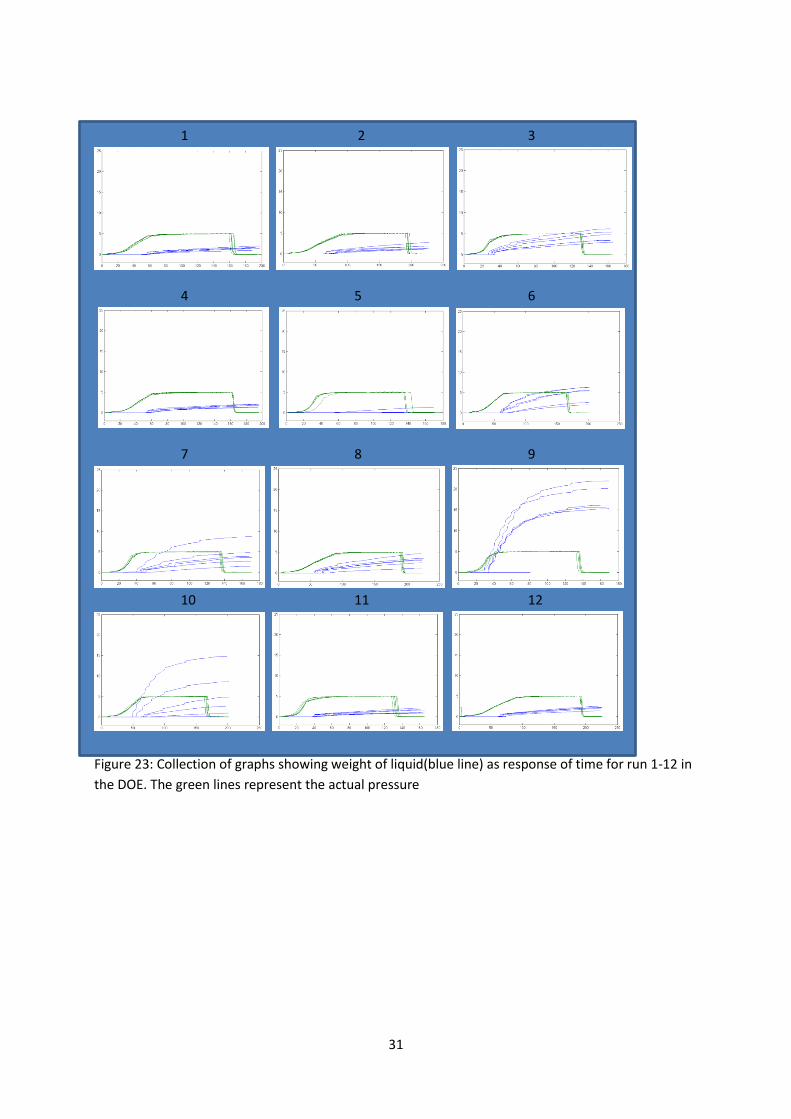
Figure 23: Collection of graphs showing weight of liquid(blue line) as response of time for run 1-12 in

the DOE. The green lines represent the actual pressure

32

13 14 15

16 17 18

19 20

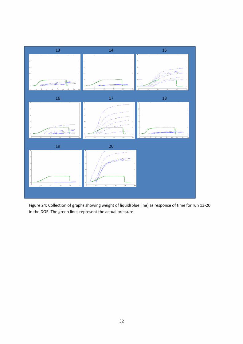
Figure 24: Collection of graphs showing weight of liquid(blue line) as response of time for run 13-20

in the DOE. The green lines represent the actual pressure

33

Table 6: All parameters included in the models, on all the different results for the DOE optimization

Rel.int

Term Coeff P-value

Constant 3,75449 0

Waiting time 0,375117 0,051

dose -0,063218 0,002

pressure increase 0,0623226 0,355

product 3,49599 0

Waiting time*pressure increase

-0,009628 0,038

Waiting time*product 0,16296 0,023

dose*product -0,064075 0,002

First P

Term Coeff P-value

Constant 7,45942 0

Waiting time 0,0723842 0,098

dose -0,064310 0

pressure increase -0,017339 0,024

product 2,31056 0,839

dose*product -0,038196 0,002

StdevP

Term Coeff P-value

Constant 8,00384 0,0001

Waiting time -1,67035 0,163

dose -0,143867 0,145

pressure increase 0,027275 0,214

product -0,0793 0,761

Waiting time*dose 0,0250438 0,046

StdevW

Term Coeff P-value

Constant -3,64888 0,004

Waiting time 0,0512023 0,032

dose 0,0503342 0,011

Pressure increase 0,0721675 0,097

Waiting time*pressure increase

-0,005791 0,038

dose*pressure increase -0,000641 0,214

Tot W Term Coeff P-value

Constant -4,59993 0

Dose 0,143083 0,004

Waiting time 0,35025 0,028

Pressure increase -0,016736 0,127

Waiting time*dose -0,008758 0,169

34

Appendix 2: The verification test

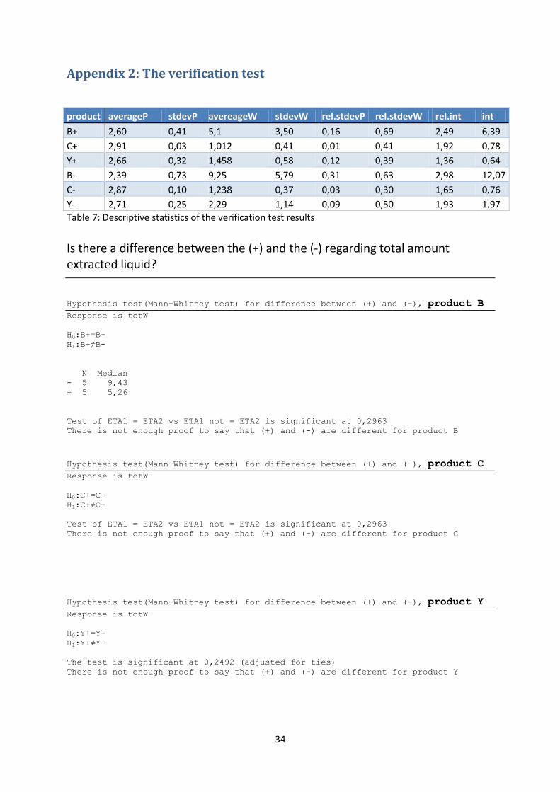
product averageP stdevP avereageW stdevW rel.stdevP rel.stdevW rel.int int

B+ 2,60 0,41 5,1 3,50 0,16 0,69 2,49 6,39

C+ 2,91 0,03 1,012 0,41 0,01 0,41 1,92 0,78

Y+ 2,66 0,32 1,458 0,58 0,12 0,39 1,36 0,64

B- 2,39 0,73 9,25 5,79 0,31 0,63 2,98 12,07

C- 2,87 0,10 1,238 0,37 0,03 0,30 1,65 0,76

Y- 2,71 0,25 2,29 1,14 0,09 0,50 1,93 1,97

Table 7: Descriptive statistics of the verification test results

Is there a difference between the (+) and the (-) regarding total amount extracted liquid?

Hypothesis test(Mann-Whitney test) for difference between (+) and (-), product B

Response is totW

H0:B+=B-

H1:B+≠B-

N Median

- 5 9,43

+ 5 5,26

Test of ETA1 = ETA2 vs ETA1 not = ETA2 is significant at 0,2963

There is not enough proof to say that (+) and (-) are different for product B

Hypothesis test(Mann-Whitney test) for difference between (+) and (-), product C

Response is totW

H0:C+=C-

H1:C+≠C-

Test of ETA1 = ETA2 vs ETA1 not = ETA2 is significant at 0,2963

There is not enough proof to say that (+) and (-) are different for product C

Hypothesis test(Mann-Whitney test) for difference between (+) and (-), product Y

Response is totW

H0:Y+=Y-

H1:Y+≠Y-

The test is significant at 0,2492 (adjusted for ties)

There is not enough proof to say that (+) and (-) are different for product Y

35

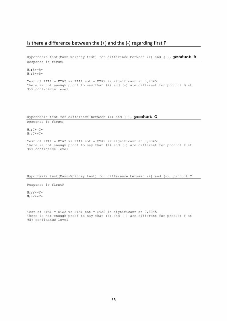
Is there a difference between the (+) and the (-) regarding first P

Hypothesis test(Mann-Whitney test) for difference between (+) and (-), product B

Response is firstP

H0:B+=B-

H1:B+≠B-

Test of ETA1 = ETA2 vs ETA1 not = ETA2 is significant at 0,8345

There is not enough proof to say that (+) and (-) are different for product B at

95% confidence level

Hypothesis test for difference between (+) and (-), product C

Response is firstP

H0:C+=C-

H1:C+≠C-

Test of ETA1 = ETA2 vs ETA1 not = ETA2 is significant at 0,8345

There is not enough proof to say that (+) and (-) are different for product Y at

95% confidence level

Hypothesis test(Mann-Whitney test) for difference between (+) and (-), product Y

Response is firstP

H0:Y+=Y-

H1:Y+≠Y-

Test of ETA1 = ETA2 vs ETA1 not = ETA2 is significant at 0,8345

There is not enough proof to say that (+) and (-) are different for product Y at

95% confidence level

36

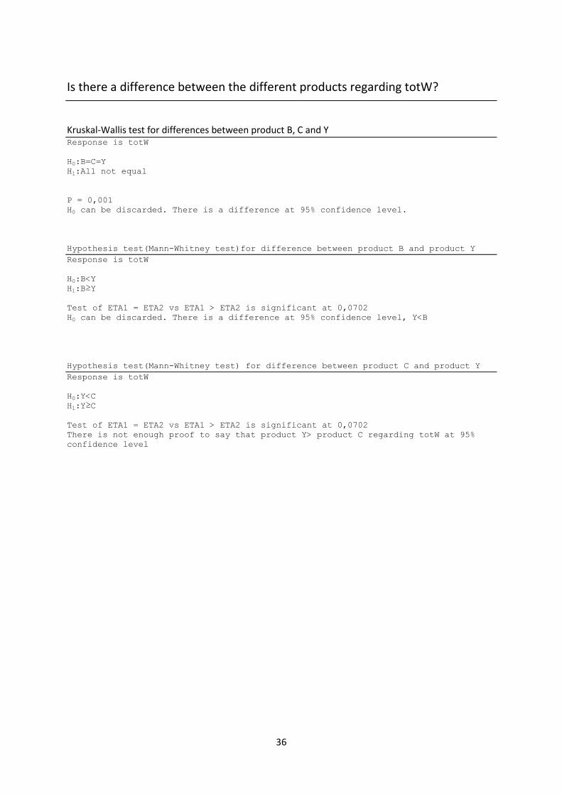
Is there a difference between the different products regarding totW?

Kruskal-Wallis test for differences between product B, C and Y Response is totW

H0:B=C=Y

H1:All not equal

P = 0,001

H0 can be discarded. There is a difference at 95% confidence level.

Hypothesis test(Mann-Whitney test)for difference between product B and product Y

Response is totW

H0:B<Y

H1:B≥Y

Test of ETA1 = ETA2 vs ETA1 > ETA2 is significant at 0,0702

H0 can be discarded. There is a difference at 95% confidence level, Y<B

Hypothesis test(Mann-Whitney test) for difference between product C and product Y

Response is totW

H0:Y<C

H1:Y≥C

Test of ETA1 = ETA2 vs ETA1 > ETA2 is significant at 0,0702

There is not enough proof to say that product Y> product C regarding totW at 95%

confidence level

37

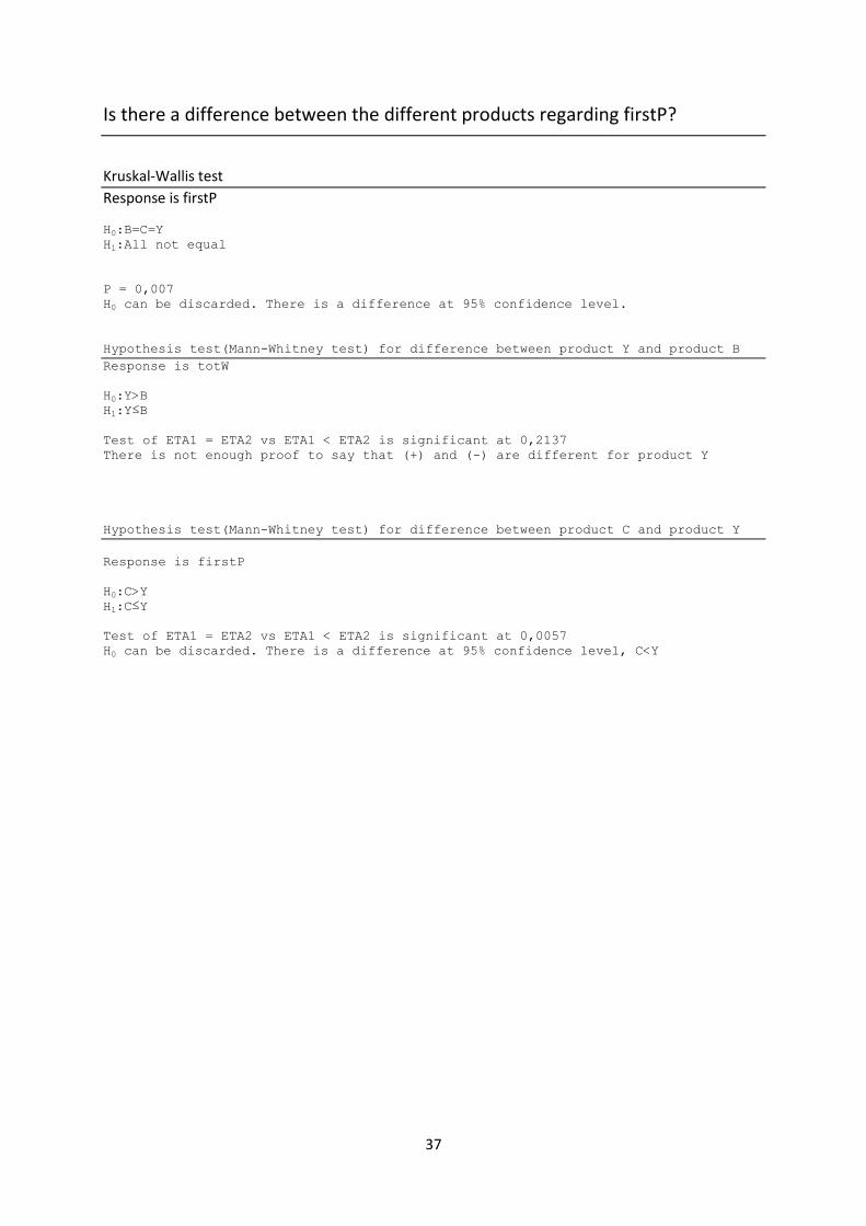
Is there a difference between the different products regarding firstP?

Kruskal-Wallis test

Response is firstP

H0:B=C=Y

H1:All not equal

P = 0,007

H0 can be discarded. There is a difference at 95% confidence level.

Hypothesis test(Mann-Whitney test) for difference between product Y and product B

Response is totW

H0:Y>B

H1:Y≤B

Test of ETA1 = ETA2 vs ETA1 < ETA2 is significant at 0,2137

There is not enough proof to say that (+) and (-) are different for product Y

Hypothesis test(Mann-Whitney test) for difference between product C and product Y

Response is firstP

H0:C>Y

H1:C≤Y

Test of ETA1 = ETA2 vs ETA1 < ETA2 is significant at 0,0057

H0 can be discarded. There is a difference at 95% confidence level, C<Y

38

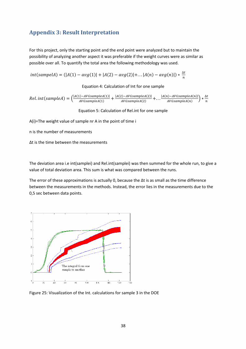
Appendix 3: Result Interpretation

For this project, only the starting point and the end point were analyzed but to maintain the

possibility of analyzing another aspect it was preferable if the weight curves were as similar as

possible over all. To quantify the total area the following methodology was used.

| | | | | |

Equation 4: Calculation of Int for one sample

(| |

| |

| |

)

Equation 5: Calculation of Rel.int for one sample

A(i)=The weight value of sample nr A in the point of time i

n is the number of measurements

∆t is the time between the measurements

The deviation area i.e int(samplei) and Rel.int(samplei) was then summed for the whole run, to give a

value of total deviation area. This sum is what was compared between the runs.

The error of these approximations is actually 0, because the ∆t is as small as the time difference

between the measurements in the methods. Instead, the error lies in the measurements due to the

0,5 sec between data points.

Figure 25: Visualization of the Int. calculations for sample 3 in the DOE

39

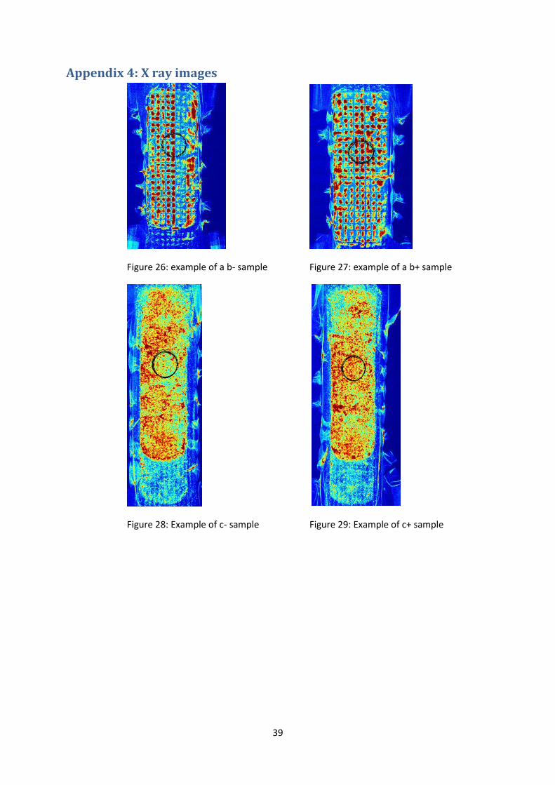
Appendix 4: X ray images

Figure 26: example of a b- sample Figure 27: example of a b+ sample

Figure 28: Example of c- sample Figure 29: Example of c+ sample

40

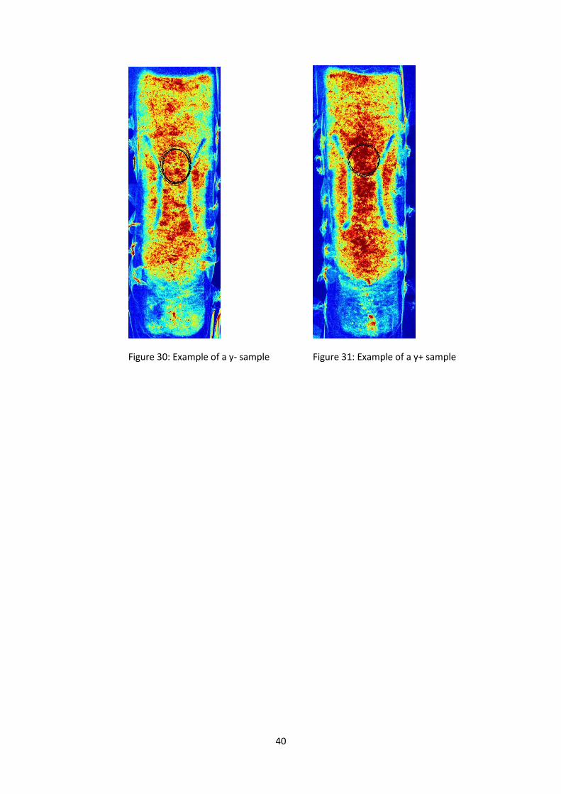
Figure 30: Example of a y- sample Figure 31: Example of a y+ sample

41

Appendix 5: Additional equations

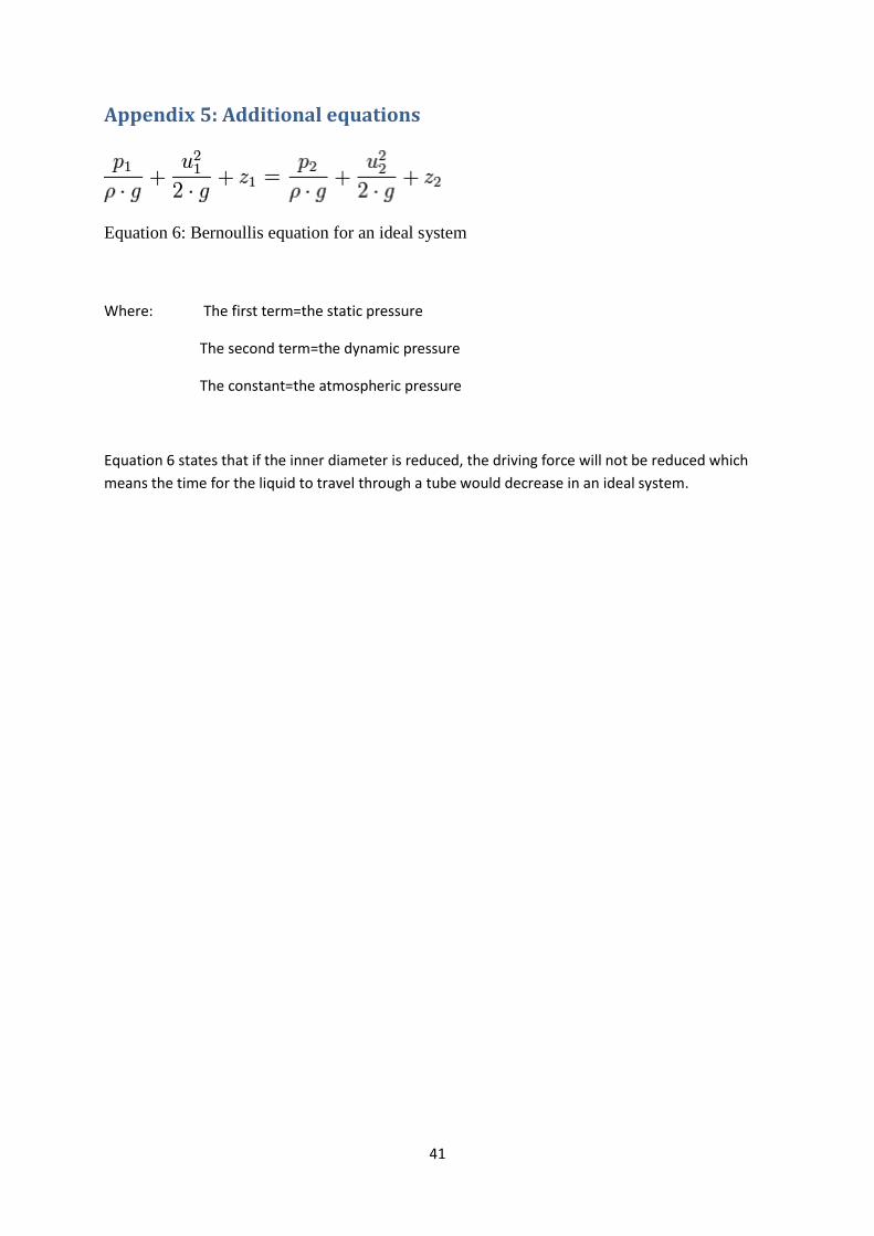
Equation 6: Bernoullis equation for an ideal system

Where: The first term=the static pressure

The second term=the dynamic pressure

The constant=the atmospheric pressure

Equation 6 states that if the inner diameter is reduced, the driving force will not be reduced which

means the time for the liquid to travel through a tube would decrease in an ideal system.