Reuse of AIP Publishing content is subject to the terms at: <a href="https://publishing.aip.org/authors/rights-and-permissions">https://publishing.aip.org/authors/rights-and-permissions</a>. Downloaded to: 131.236.54.139 on 28 November 2018, At: 14:56

Measuring monopole and dipole polarizability of acoustic meta-atomsJoshua Jordaan, Stefan Punzet, Anton Melnikov, Alexandre Sanches, Sebastian Oberst, Steffen Marburg, andDavid A. Powell

Citation: Appl. Phys. Lett. 113, 224102 (2018); doi: 10.1063/1.5052661View online: https://doi.org/10.1063/1.5052661View Table of Contents: http://aip.scitation.org/toc/apl/113/22Published by the American Institute of Physics

Measuring monopole and dipole polarizability of acoustic meta-atoms

Joshua Jordaan,1 Stefan Punzet,1,2,3 Anton Melnikov,4,5,6 Alexandre Sanches,1,7

Sebastian Oberst,5 Steffen Marburg,4 and David A. Powell1,6,a)

1Nonlinear Physics Centre, Research School of Physics and Engineering, The Australian National University,Canberra, ACT 2601, Australia2Faculty of Electrical Engineering and Information Technology, Ostbayerische Technische HochschuleRegensburg, Seybothstraße 2, 93053 Regensburg, Germany3Department of Electrical and Computer Engineering, Technical University of Munich, Theresienstr. 90,80333 Munich, Germany4Vibroacoustics of Vehicles and Machines, Technical University of Munich, Boltzmann Str. 15,85748 Garching, Germany5Centre for Audio, Acoustics and Vibration, University of Technology Sydney, NSW 2007, Australia6School of Engineering and Information Technology, University of New South Wales, Canberra, ACT 2610,Australia7School of Engineering, University of S~ao Paulo, Av. Prof. Luciano Gualberto, 380 - Butant~a,CEP 05508-010 S~ao Paulo, SP, Brazil

(Received 20 August 2018; accepted 8 November 2018; published online 28 November 2018)

We present a method to extract monopole and dipole polarizability from experimental

measurements of two-dimensional acoustic meta-atoms. In contrast to extraction from numerical

results, this enables all second-order effects and uncertainties in material properties to be accounted

for. We apply the technique to 3D-printed labyrinthine meta-atoms of a variety of geometries. We

show that the polarizability of structures with a shorter acoustic path length agrees well with

numerical results. However, those with longer path lengths suffer strong additional damping, which

we attribute to the strong viscous and thermal losses in narrow channels. Published by AIPPublishing. https://doi.org/10.1063/1.5052661

Acoustic metasurfaces are metamaterial structures with

sub-wavelength thickness that can implement a rich variety

of acoustic functions.1,2 A promising approach for metasur-

faces is the design of structures with the internal labyrinthine

configuration to slow down the acoustic wave’s velocity to

create compact resonators.3,4 Structures of this kind exhibit

excellent wavefront shaping potential.1,5–7 Such meta-atoms

can generate phase shifts up to 2p by adjusting their geome-

try.5 Thereby, a wave manipulation function can be realized

with the corresponding phase gradient, which is then discre-

tized to enable implementation with an array of meta-atoms.

Drawing inspiration from electromagnetism, the

dominant design paradigm for acoustic metasurfaces has

been the generalized Snell’s law,6,8 where structures are

designed for high amplitude, with spatially varying phases,

for both transmission and reflection problems. However, in

electromagnetism, it has been shown that the generalized

Snell’s law does not correctly account for impedance match-

ing and energy conservation. Approaches based on surface

impedance must be used instead,9,10 and equivalent electric

and magnetic surface impedances need to be defined.

Recently, these more accurate surface-impedance models

have also been applied to acoustic metasurfaces.12,13 The

impedances can be derived from the multipole moments of a

single meta-atom.11 In the acoustics of fluids, the fundamen-

tal moments are the monopole and dipole, corresponding to

the net compression and displacement of a fluid volume,

respectively. The acoustic response of sub-wavelength

meta-atoms is well-approximated by their monopole and

dipole polarizability coefficients. These coefficients relate

the strength of the monopole and dipole moments to the

incident pressure and velocity fields, respectively.

Developing a model based on polarizability can lead to great

simplifications in modelling, particularly for complex

arrangements of meta-atoms.

An alternative to a continuously connected metasurface

is the use of sparse arrays of disconnected resonant meta-

atoms,1,14 which can enable highly efficient beam refraction

at large angles.15 These elements may find their application

in creating sound control structures which also allow airflow.

Here, the monopole and dipole polarizabilities of the

meta-atoms are the most natural model to apply. To date,

these polarizabilities have not been directly measured; with

most designs relying on simulations or indirect observations

of resonances attributed to the monopolar and dipolar

modes.14,16

In this work, we present a technique for directly extract-

ing the acoustic monopole and dipole polarizability of two-

dimensional meta-atoms from experimental measurements.

In addition, the method can be applied to numerically

extracted data. Obtaining polarizability information from

experimental measurements is necessary for good accuracy,

since numerical simulation may neglect viscous and thermal

boundary layers and the excitation of vibration modes in thin

structures, and it may be difficult to obtain reliable material

properties for rapid prototyping materials.

In this work, we consider the experimental configuration

shown in Fig. 1, similar to that used in previous works.6,17

Two plates separated by a 66 mm gap form a parallel-plate

acoustic waveguide, with uniform pressure distribution ina)Electronic mail: david.powell@adfa.edu.au

0003-6951/2018/113(22)/224102/5/$30.00 Published by AIP Publishing.113, 224102-1

APPLIED PHYSICS LETTERS 113, 224102 (2018)

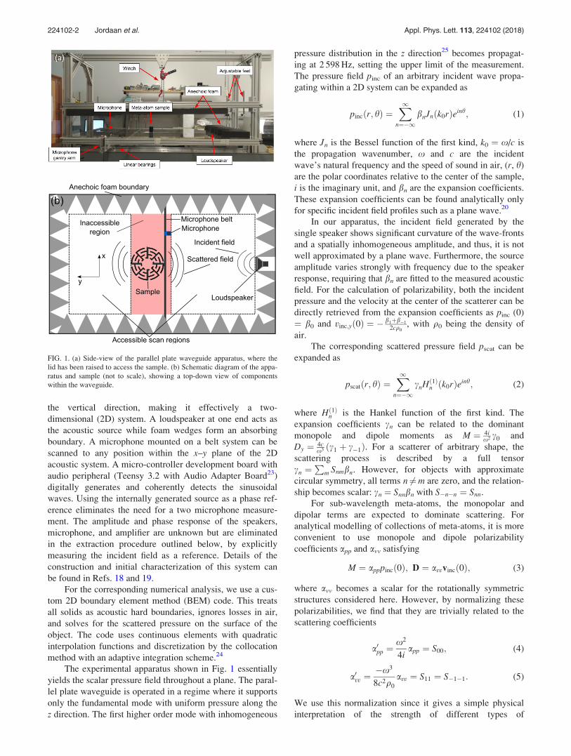
the vertical direction, making it effectively a two-

dimensional (2D) system. A loudspeaker at one end acts as

the acoustic source while foam wedges form an absorbing

boundary. A microphone mounted on a belt system can be

scanned to any position within the x–y plane of the 2D

acoustic system. A micro-controller development board with

audio peripheral (Teensy 3.2 with Audio Adapter Board23)

digitally generates and coherently detects the sinusoidal

waves. Using the internally generated source as a phase ref-

erence eliminates the need for a two microphone measure-

ment. The amplitude and phase response of the speakers,

microphone, and amplifier are unknown but are eliminated

in the extraction procedure outlined below, by explicitly

measuring the incident field as a reference. Details of the

construction and initial characterization of this system can

be found in Refs. 18 and 19.

For the corresponding numerical analysis, we use a cus-

tom 2D boundary element method (BEM) code. This treats

all solids as acoustic hard boundaries, ignores losses in air,

and solves for the scattered pressure on the surface of the

object. The code uses continuous elements with quadratic

interpolation functions and discretization by the collocation

method with an adaptive integration scheme.24

The experimental apparatus shown in Fig. 1 essentially

yields the scalar pressure field throughout a plane. The paral-

lel plate waveguide is operated in a regime where it supports

only the fundamental mode with uniform pressure along the

z direction. The first higher order mode with inhomogeneous

pressure distribution in the z direction25 becomes propagat-

ing at 2 598 Hz, setting the upper limit of the measurement.

The pressure field pinc of an arbitrary incident wave propa-

gating within a 2D system can be expanded as

pincðr; hÞ ¼X1

n¼�1bnJnðk0rÞeinh; (1)

where Jn is the Bessel function of the first kind, k0 ¼ x/c is

the propagation wavenumber, x and c are the incident

wave’s natural frequency and the speed of sound in air, (r, h)

are the polar coordinates relative to the center of the sample,

i is the imaginary unit, and bn are the expansion coefficients.

These expansion coefficients can be found analytically only

for specific incident field profiles such as a plane wave.20

In our apparatus, the incident field generated by the

single speaker shows significant curvature of the wave-fronts

and a spatially inhomogeneous amplitude, and thus, it is not

well approximated by a plane wave. Furthermore, the source

amplitude varies strongly with frequency due to the speaker

response, requiring that bn are fitted to the measured acoustic

field. For the calculation of polarizability, both the incident

pressure and the velocity at the center of the scatterer can be

directly retrieved from the expansion coefficients as pinc (0)

¼ b0 and vinc;yð0Þ ¼ � b1þb�1

2cq0, with q0 being the density of

air.

The corresponding scattered pressure field pscat can be

expanded as

pscatðr; hÞ ¼X1

n¼�1cnHð1Þn ðk0rÞeinh; (2)

where Hð1Þn is the Hankel function of the first kind. The

expansion coefficients cn can be related to the dominant

monopole and dipole moments as M ¼ 4ix2 c0 and

Dy ¼ 4cx3 ðc1 þ c�1Þ. For a scatterer of arbitrary shape, the

scattering process is described by a full tensor

cn ¼P

m Snmbn. However, for objects with approximate

circular symmetry, all terms n 6¼m are zero, and the relation-

ship becomes scalar: cn ¼ Snnbn with S�n�n ¼ Snn.

For sub-wavelength meta-atoms, the monopolar and

dipolar terms are expected to dominate scattering. For

analytical modelling of collections of meta-atoms, it is more

convenient to use monopole and dipole polarizability

coefficients app and avv satisfying

M ¼ apppincð0Þ; D ¼ avvvincð0Þ; (3)

where avv becomes a scalar for the rotationally symmetric

structures considered here. However, by normalizing these

polarizabilities, we find that they are trivially related to the

scattering coefficients

a0pp ¼x2

4iapp ¼ S00; (4)

a0vv ¼�x3

8c2q0

avv ¼ S11 ¼ S�1�1: (5)

We use this normalization since it gives a simple physical

interpretation of the strength of different types of

FIG. 1. (a) Side-view of the parallel plate waveguide apparatus, where the

lid has been raised to access the sample. (b) Schematic diagram of the appa-

ratus and sample (not to scale), showing a top-down view of components

within the waveguide.

224102-2 Jordaan et al. Appl. Phys. Lett. 113, 224102 (2018)

polarizabilities in terms of contribution to scattering, with a

maximum magnitude of unity.

To experimentally measure the acoustic polarizability,

we need to determine the incident field coefficients bn and

the scattered field coefficients cn for n 2 {0, 1, �1}. The

incident field is measured on a circle of radius Rinc. Applying

the orthogonality of exponential functions to Eq. (1), we find

the incident field coefficients as

bn ¼1

2pJnðk0RincÞ

ðp

�ppincðRinc; hÞe�inhdh: (6)

Note that the Bessel functions have zeros which make Eq.

(6) singular, the first of which occurs at k0Rinc � 2.4. Thus,

Rinc is chosen sufficiently small to remain well below this

singular condition at the highest frequency of interest.

For determination of the scattered field coefficients, we

measure both the total field ptot and incident field pinc at the

same radius Rscat, with the scattered field given by their dif-

ference pscat ¼ ptot � pinc. Integrating Eq. (2) and applying

orthogonality conditions, the scattered field coefficients are

given by

cn ¼1

2pHð1Þn ðk0RscatÞ

ðp

�ppscatðRscat; hÞe�inhdh: (7)

As the Hankel function has no real zeros, there is more

freedom to choose Rscat. Referring to Fig. 1(b), we see that

when the sample is placed within the waveguide, there is an

inaccessible region of width w where the field cannot be

measured, as the belt on which the microphone is mounted

would collide with the sample. Therefore, we must measure

over a reduced angular range and approximate the angular

integral as

1

2p

ð2p

0

� � � dh � 1

2p� 4hin

ðp�hin

hin

� � � dhþð2p�hin

pþhin

� � � dh

!;

(8)

where hin ¼ arcsin w2Rscat

is the angular half-width of the

inaccessible region. Since the range of inaccessible angles

reduces with increasing Rscat, larger values are preferred for

increased accuracy. This reduced angular range of

integration means that we do not have exact orthogonality

between different orders n. However, for sub-wavelength

meta-atoms with dominant monopolar and dipolar radiation,

the scattered field will have relatively smooth angular varia-

tion, and we do not expect significant interference from

higher order terms with jnj > 1.

The ratio of the scattered field coefficients cn to the inci-

dent field coefficients bn gives the corresponding scattering

coefficient Snn according to Eqs. (4) and (5). Since we have

two equivalent expressions for the dipole polarizability a0vv,their average is taken to reduce the influence of measurement

uncertainties.

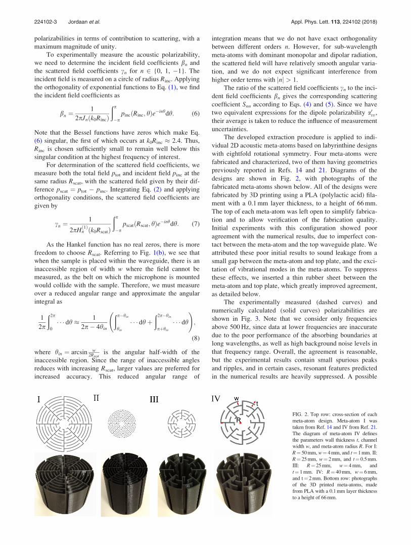
The developed extraction procedure is applied to indi-

vidual 2D acoustic meta-atoms based on labyrinthine designs

with eightfold rotational symmetry. Four meta-atoms were

fabricated and characterized, two of them having geometries

previously reported in Refs. 14 and 21. Diagrams of the

designs are shown in Fig. 2, with photographs of the

fabricated meta-atoms shown below. All of the designs were

fabricated by 3D printing using a PLA (polylactic acid) fila-

ment with a 0.1 mm layer thickness, to a height of 66 mm.

The top of each meta-atom was left open to simplify fabrica-

tion and to allow verification of the fabrication quality.

Initial experiments with this configuration showed poor

agreement with the numerical results, due to imperfect con-

tact between the meta-atom and the top waveguide plate. We

attributed these poor initial results to sound leakage from a

small gap between the meta-atom and top plate, and the exci-

tation of vibrational modes in the meta-atoms. To suppress

these effects, we inserted a thin rubber sheet between the

meta-atom and top plate, which greatly improved agreement,

as detailed below.

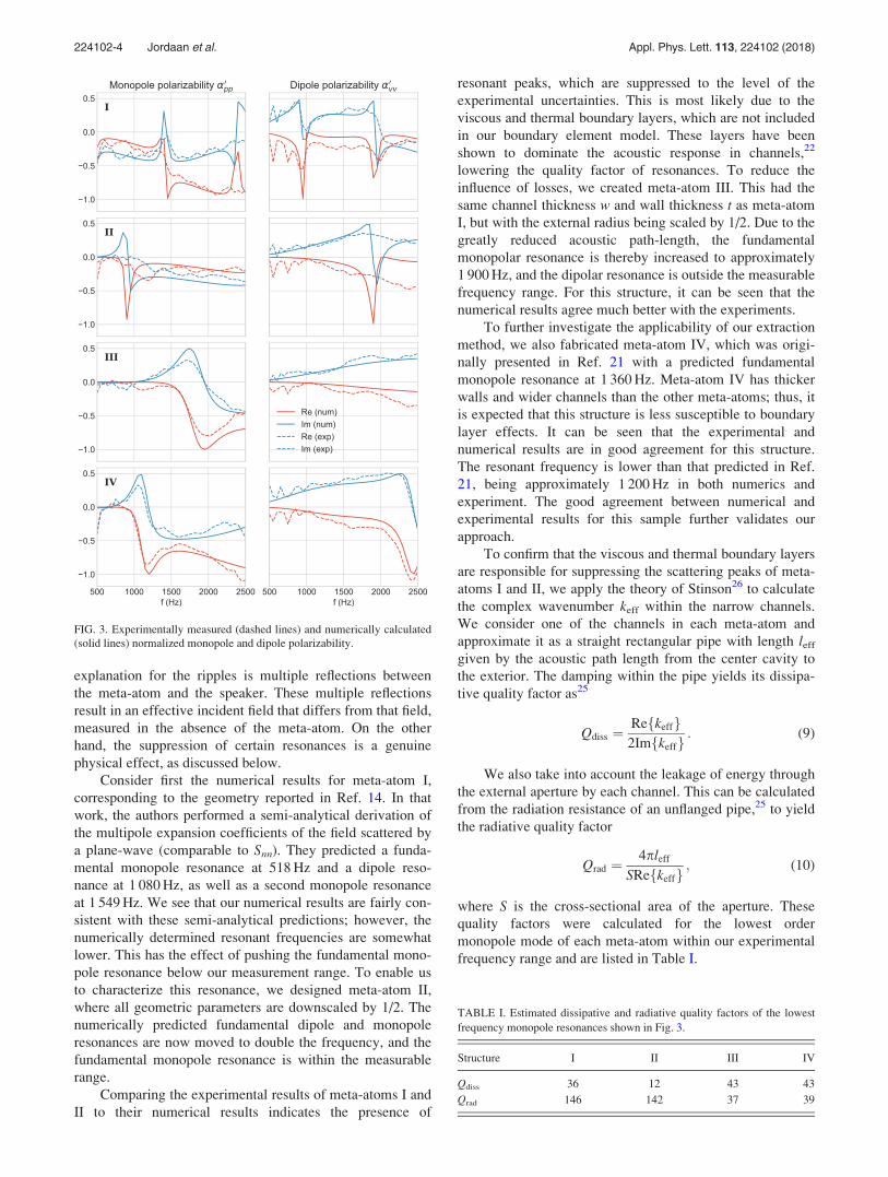
The experimentally measured (dashed curves) and

numerically calculated (solid curves) polarizabilities are

shown in Fig. 3. Note that we consider only frequencies

above 500 Hz, since data at lower frequencies are inaccurate

due to the poor performance of the absorbing boundaries at

long wavelengths, as well as high background noise levels in

that frequency range. Overall, the agreement is reasonable,

but the experimental results contain small spurious peaks

and ripples, and in certain cases, resonant features predicted

in the numerical results are heavily suppressed. A possible

FIG. 2. Top row: cross-section of each

meta-atom design. Meta-atom I was

taken from Ref. 14 and IV from Ref. 21.

The diagram of meta-atom IV defines

the parameters wall thickness t, channel

width w, and meta-atom radius R. For I:

R¼ 50 mm, w¼ 4 mm, and t¼ 1 mm. II:

R¼ 25 mm, w¼ 2 mm, and t¼ 0.5 mm.

III: R¼ 25 mm, w¼ 4 mm, and

t¼ 1 mm. IV: R¼ 40 mm, w¼ 6 mm,

and t¼ 2 mm. Bottom row: photographs

of the 3D printed meta-atoms, made

from PLA with a 0.1 mm layer thickness

to a height of 66 mm.

224102-3 Jordaan et al. Appl. Phys. Lett. 113, 224102 (2018)

explanation for the ripples is multiple reflections between

the meta-atom and the speaker. These multiple reflections

result in an effective incident field that differs from that field,

measured in the absence of the meta-atom. On the other

hand, the suppression of certain resonances is a genuine

physical effect, as discussed below.

Consider first the numerical results for meta-atom I,

corresponding to the geometry reported in Ref. 14. In that

work, the authors performed a semi-analytical derivation of

the multipole expansion coefficients of the field scattered by

a plane-wave (comparable to Snn). They predicted a funda-

mental monopole resonance at 518 Hz and a dipole reso-

nance at 1 080 Hz, as well as a second monopole resonance

at 1 549 Hz. We see that our numerical results are fairly con-

sistent with these semi-analytical predictions; however, the

numerically determined resonant frequencies are somewhat

lower. This has the effect of pushing the fundamental mono-

pole resonance below our measurement range. To enable us

to characterize this resonance, we designed meta-atom II,

where all geometric parameters are downscaled by 1/2. The

numerically predicted fundamental dipole and monopole

resonances are now moved to double the frequency, and the

fundamental monopole resonance is within the measurable

range.

Comparing the experimental results of meta-atoms I and

II to their numerical results indicates the presence of

resonant peaks, which are suppressed to the level of the

experimental uncertainties. This is most likely due to the

viscous and thermal boundary layers, which are not included

in our boundary element model. These layers have been

shown to dominate the acoustic response in channels,22

lowering the quality factor of resonances. To reduce the

influence of losses, we created meta-atom III. This had the

same channel thickness w and wall thickness t as meta-atom

I, but with the external radius being scaled by 1/2. Due to the

greatly reduced acoustic path-length, the fundamental

monopolar resonance is thereby increased to approximately

1 900 Hz, and the dipolar resonance is outside the measurable

frequency range. For this structure, it can be seen that the

numerical results agree much better with the experiments.

To further investigate the applicability of our extraction

method, we also fabricated meta-atom IV, which was origi-

nally presented in Ref. 21 with a predicted fundamental

monopole resonance at 1 360 Hz. Meta-atom IV has thicker

walls and wider channels than the other meta-atoms; thus, it

is expected that this structure is less susceptible to boundary

layer effects. It can be seen that the experimental and

numerical results are in good agreement for this structure.

The resonant frequency is lower than that predicted in Ref.

21, being approximately 1 200 Hz in both numerics and

experiment. The good agreement between numerical and

experimental results for this sample further validates our

approach.

To confirm that the viscous and thermal boundary layers

are responsible for suppressing the scattering peaks of meta-

atoms I and II, we apply the theory of Stinson26 to calculate

the complex wavenumber keff within the narrow channels.

We consider one of the channels in each meta-atom and

approximate it as a straight rectangular pipe with length leff

given by the acoustic path length from the center cavity to

the exterior. The damping within the pipe yields its dissipa-

tive quality factor as25

Qdiss ¼Refkeffg2Imfkeffg

: (9)

We also take into account the leakage of energy through

the external aperture by each channel. This can be calculated

from the radiation resistance of an unflanged pipe,25 to yield

the radiative quality factor

Qrad ¼4pleff

SRefkeffg; (10)

where S is the cross-sectional area of the aperture. These

quality factors were calculated for the lowest order

monopole mode of each meta-atom within our experimental

frequency range and are listed in Table I.

FIG. 3. Experimentally measured (dashed lines) and numerically calculated

(solid lines) normalized monopole and dipole polarizability.

TABLE I. Estimated dissipative and radiative quality factors of the lowest

frequency monopole resonances shown in Fig. 3.

Structure I II III IV

Qdiss 36 12 43 43

Qrad 146 142 37 39

224102-4 Jordaan et al. Appl. Phys. Lett. 113, 224102 (2018)

The dissipative and radiative quality factors can be com-

bined to find the total quality factor Qtot ¼ ðQ�1diss þ Q�1

rad�1

,

which determines the total rate of energy loss from the

cavity. However, to interpret the scattering response, we

need to consider the individual contribution from each of

these terms. By reciprocity, the radiative quality factor Qrad

also determines how long it takes an incident wave to couple

into the structure. Qdiss determines the time scale over which

energy is dissipated internally. If Qdiss � Qrad, then internal

dissipation will dominate over radiation of energy, and reso-

nant scattering will be suppressed. As can be seen in Table I,

for meta-atoms I and II, internal dissipation dominates over

radiation, which explains the strong suppression of the

resonant scattering peaks. In contrast, for meta-atoms III and

IV, radiative and dissipative losses are comparable, and thus,

the experimentally observed scattering is only moderately

suppressed compared to the simulated values.

In conclusion, we presented a method for extracting the

monopole and dipole polarizability from experimental mea-

surements of two-dimensional acoustic meta-atoms. We

applied this method to labyrinthine meta-atoms previously

reported in the literature. For structures with thin walls and

long acoustic path lengths, the resonances predicted numeri-

cally were highly damped and were essentially unobservable

in the experiment. We attribute this to the viscous and ther-

mal boundary layers, which have a thickness comparable to

the width of the narrow channels. When applying our method

to structures with shorter acoustic path lengths and wider

channels, we found good agreement with numerical results.

We acknowledge useful discussions with Andrea Al�uand Li Quan. A.M. acknowledges the financial support

provided by S.O. over the UTS Centre for Audio, Acoustics

and Vibration (CAAV) international visitor funds. D.P.

acknowledges funding from the Australian Research Council

through Discovery Project No. DP150103611.

1J. Zhao, Manipulation of Sound Properties by Acoustic Metasurface andMetastructure, Springer Theses (Springer Singapore, Singapore, 2016).

2S. A. Cummer, J. Christensen, and A. Al�u, “Controlling sound with acous-

tic metamaterials,” Nature Rev. Mater. 1, 16001 (2016).3Z. Liang and J. Li, “Extreme acoustic metamaterial by coiling up space,”

Phys. Rev. Lett. 108, 114301 (2012).4Y. Xie, A. Konneker, B.-I. Popa, and S. A. Cummer, “Tapered

labyrinthine acoustic metamaterials for broadband impedance matching,”

Appl. Phys. Lett. 103, 201906 (2013).5C. Shen, “Design of acoustic metamaterials and metasurfaces,” Ph.D. the-

sis (North Carolina State University, Raleigh, North Carolina, 2016).

6Y. Li, X. Jiang, R.-Q. Li, B. Liang, X.-Y. Zou, L.-L. Yin, and J.-C. Cheng,

“Experimental realization of full control of reflected waves with subwave-

length acoustic metasurfaces,” Phys. Rev. Appl. 2, 064002 (2014).7Y. Xie, W. Wang, H. Chen, A. Konneker, B.-I. Popa, and S. A. Cummer,

“Wavefront modulation and subwavelength diffractive acoustics with an

acoustic metasurface,” Nat. Commun. 5, 5553 (2014).8K. Tang, C. Qiu, M. Ke, J. Lu, Y. Ye, and Z. Liu, “Anomalous refraction of

airborne sound through ultrathin metasurfaces,” Sci. Rep. 4, 6517 (2014).9K. Achouri, M. A. Salem, and C. Caloz, “General metasurface synthesis

based on susceptibility tensors,” IEEE Trans. Antennas Propag. 63,

2977–2991 (2015).10N. M. Estakhri and A. Al�u, “Wave-front transformation with gradient

metasurfaces,” Phys. Rev. X 6, 041008 (2016).11E. F. Kuester, M. A. Mohamed, M. Piket-May, and C. L. Holloway,

“Averaged transition conditions for electromagnetic fields at a metafilm,”

IEEE Trans. Antennas Propag. 51, 2641–2651 (2003).12A. D�ıaz-Rubio and S. A. Tretyakov, “Acoustic metasurfaces for

scattering-free anomalous reflection and refraction,” Phys. Rev. B 96,

125409 (2017).13J. Li, C. Shen, A. D�ıaz-Rubio, S. A. Tretyakov, and S. A. Cummer,

“Systematic design and experimental demonstration of bianisotropic meta-

surfaces for scattering-free manipulation of acoustic wavefronts,” Nat.

Commun. 9, 1342 (2018).14Y. Cheng, C. Zhou, B. G. Yuan, D. J. Wu, Q. Wei, and X. J. Liu, “Ultra-

sparse metasurface for high reflection of low-frequency sound based on

artificial Mie resonances,” Nat. Mater. 14, 1013–1019 (2015).15L. Quan, Y. Ra’di, D. L. Sounas, and A. Al�u, “Maximum Willis coupling

in acoustic scatterers,” Phys. Rev. Lett. 120, 254301 (2018).16A. O. Krushynska, F. Bosia, M. Miniaci, and N. M. Pugno, “Spider web-

structured labyrinthine acoustic metamaterials for low-frequency sound

control,” New J. Phys. 19, 105001 (2017).17L. Zigoneanu, B.-I. Popa, and S. A. Cummer, “Design and measurements

of a broadband two-dimensional acoustic lens,” Phys. Rev. B 84, 024305

(2011).18J. Jordaan, “Acoustic meta-atoms: An experimental determination of the

monopole and dipole scattering coefficients,” Final year project thesis

(Australian National University, 2017).19S. Punzet, “Design and construction of an acoustic scanning stage,”

Internship report (Ostbayerische Technische Hochschule Regensburg,

University of Applied Science, 2016).20C. C. Mei, Mathematical Analysis in Engineering: How to Use the Basic

Tools (Cambridge University Press, Cambridge, 1997).21G. Lu, E. Ding, Y. Wang, X. Peng, J. Cui, X. Liu, and X. Liu, “Realization

of acoustic wave directivity at low frequencies with a subwavelength Mie

resonant structure,” Appl. Phys. Lett. 110, 123507 (2017).22G. P. Ward, R. K. Lovelock, A. R. J. Murray, A. P. Hibbins, J. R. Sambles,

and J. D. Smith, “Boundary-layer effects on acoustic transmission through

narrow slit cavities,” Phys. Rev. Lett. 115, 044302 (2015).23See https://www.pjrc.com/store/teensy3_audio.html for Audio adaptor

board for Teensy 3.0 – 3.6.24S. Marburg, “Boundary element method for time-harmonic acoustic prob-

lems,” in Computational Acoustics, CISM International Centre for

Mechanical Sciences Vol. 579, edited by M. Kaltenbacher (Springer,

Cham, 2018), pp. 69–158.25L. E. Kinsler, A. R. Frey, A. B. Coppens, and J. V. Sanders, Fundamentals

of Acoustics (John Wiley & Sons, 2000).26M. R. Stinson, “The propagation of plane sound waves in narrow and wide

circular tubes, and generalization to uniform tubes of arbitrary cross-sec-

tional shape,” J. Acoust. Soc. Am. 89, 550–558 (1991).

224102-5 Jordaan et al. Appl. Phys. Lett. 113, 224102 (2018)