MEASURING LIQUEFIED RESIDUAL STRENGTH USING FULL …
145
MEASURING LIQUEFIED RESIDUAL STRENGTH USING FULL-SCALE SHAKE TABLE CYCLIC SIMPLE SHEAR TESTS A Thesis Presented to The Faculty of California Polytechnic State University, San Luis Obispo In Partial Fulfillment Of the Requirements for the Degree Master of Science in Civil and Environmental Engineering By Taylor Ryan Honnette November 2018
Transcript of MEASURING LIQUEFIED RESIDUAL STRENGTH USING FULL …

MEASURING LIQUEFIED RESIDUAL STRENGTH USING FULL-SCALE
SHAKE TABLE CYCLIC SIMPLE SHEAR TESTS
A Thesis
Presented to
The Faculty of California Polytechnic State University,
San Luis Obispo
In Partial Fulfillment
Of the Requirements for the Degree
Master of Science in Civil and Environmental Engineering
By
Taylor Ryan Honnette
November 2018

ii
© 2018
Taylor Ryan Honnette
ALL RIGHTS RESERVED

iii
COMMITTEE MEMBERSHIP
TITLE: Measuring Liquefied Residual Strength Using
Full-Scale Shake Table Cyclic Simple Shear
Tests
AUTHOR: Taylor Ryan Honnette
DATE SUBMITTED: November 2018
COMMITTEE CHAIR: Dr. Robb Moss, Ph.D., PE, F.ASCE
Professor of Civil Engineering
COMMITTEE MEMBER: Mr. Nephi Derbidge
Lecturer of Civil Engineering
COMMITTEE MEMBER: Dr. Gregg Fiegel, Ph.D., PE, GE
Professor of Civil Engineering

iv
ABSTRACT
Measuring Liquefied Residual Strength Using Full-Scale Shake Table
Cyclic Simple Shear Tests
Taylor Ryan Honnette
This research consists of full-scale cyclic shake table tests to investigate
liquefied residual strength of #2/16 Monterey Sand. A simple shear testing
apparatus was mounted to a full-scale one-dimensional shake table to
mimic a confined layer of saturated sand subjected to strong ground
motions. Testing was performed at the Parson’s Geotechnical and
Earthquake Laboratory at California Polytechnic State University, San Luis
Obispo. T-bar penetrometer pullout tests were used to measure residual
strength of the liquefied soil during cyclic testing. Cone Penetration Testing
(CPT) was performed on the soil specimen throughout testing to relate the
laboratory specimen to field index test data and to compare CPT results of
the #2/16 Monterey sand before and after liquefaction. The generation and
dissipation of excess pore pressures during cyclic motion are measured and
discussed. The effects of liquefied soil on seismic ground motion are
investigated. Measured residual strengths are compared to previous
correlations comparing liquefied residual strength ratios and CPT tip
resistance.

v
ACKNOWLEDGMENTS
Foremost, I would like to thank my advisor, Dr. Robb Moss, for his constant
guidance and input throughout this research. His thoughtful
recommendations and analyses proved invaluable to this project. I am truly
appreciative for all the extra time and support Dr. Moss invested into my
education.
Mr. Derbidge’s expertise in geotechnical laboratory testing was heavily
utilized throughout this process. His ability to quickly and thoughtfully
answer my constant inquiries regarding laboratory testing and soil
mechanics were vital to this investigation.
Dr. Fiegel’s commitment to educational and engineering excellence is
evident in his courses and feedback. His courses provided me with a strong
understanding of the fundamentals of geotechnical engineering.
The Cal Poly Civil Engineering Department faculty and staff provided the
necessary materials to complete this research. Special consideration given
to: Ron Leverett, Amy Sinclair, Dr. Charles Chadwell, and Xi Shen.
Lastly, I would like to thank my fellow students for their assistance in
transporting and constructing materials and equipment used in this
research: Brock Andrew, Cory Wallace, Austin Della, and Kyle Kao.
Thank you all for your dedication and support.

vi
TABLE OF CONTENTS
LIST OF TABLES ..................................................................................... vii
LIST OF FIGURES ..................................................................................... x
CHAPTER
1. LITERATURE REVIEW ......................................................................... 1
1.1 Overview ...................................................................................... 1
1.2 Seismically-induced liquefaction mechanics ................................. 2
1.3 Liquefaction Triggering ................................................................. 3
1.4 Residual Strength Estimation ....................................................... 9
1.4.1 Case History .......................................................................... 9
1.4.2 Laboratory Testing ............................................................... 14
1.5 T-Bar Penetrometers .................................................................. 20
1.6 Full-Scale Shake Table Testing .................................................. 22
2. EQUIPMENT AND INSTRUMENTATION ........................................... 25
2.1 Load Cell .................................................................................... 25
2.2 Cone Penetrometer .................................................................... 27
2.3 T-bar Penetrometer .................................................................... 29
2.4 Accelerometers .......................................................................... 32
2.5 Pore Pressure Transducers ........................................................ 33
2.6 Tactile Pressure Sensors ........................................................... 35
2.7 Backup overburden estimation ................................................... 35
2.8 Displacement Transducers ......................................................... 35
2.9 Flexible Walled Testing Apparatus ............................................. 36
3. PRE-TESTS ........................................................................................ 39
3.1 Dry Pluviated Trash Can Test .................................................... 39
3.2 Wet Pluviated Trash Can Test 1 ................................................. 46
3.3 Wet Pluviated Trash Can Test 2 ................................................. 51
3.4 Shake Table Transfer Function .................................................. 52

vii
4. MODEL PREPARATION ..................................................................... 54
4.1 Bucket Waterproofing ................................................................. 54
4.2 Clay Placement .......................................................................... 55
4.3 Sand Placement ......................................................................... 56
4.4 Overburden Assembly ................................................................ 61
4.5 Instrument Embedment .............................................................. 65
5. TESTING ......................................................................................... 69
5.1.1 Pre-Liquefaction Shear Wave Velocity ................................. 69
5.1.2 Initial Cone Penetration Test Sounding (CPT_1.1) .............. 71
5.1.3 Cyclic Test 1.1 ..................................................................... 75
5.1.4 CPT_1.2 ............................................................................... 78
5.1.5 Cyclic Test 1.2 ..................................................................... 82
5.1.6 Cyclic Test 1.3 ..................................................................... 84
5.1.7 CPT_1.3 ............................................................................... 85
5.2 Setup 2 ....................................................................................... 88
5.2.1 CPT_2.1 ............................................................................... 88
5.2.2 Cyclic Test 2.1 ..................................................................... 92
5.2.3 CPT_2.2 ............................................................................... 95
5.2.4 Cyclic Test 2.2 ..................................................................... 98
5.2.5 CPT_2.3 ............................................................................. 100
6. RESULTS .......................................................................................... 103
6.1 Data Acquisition ....................................................................... 103
6.2 CPT Summary .......................................................................... 104
6.3 T-Bar Penetrometer Summary ................................................. 105
6.4 Pore Pressure Dissipation ........................................................ 108
6.5 Liquefied Soil Effects on Motion ............................................... 109
6.6 Liquefied Residual Strength Estimation .................................... 112
6.1.1 Cyclic Test 1.1 ................................................................... 115
6.1.2 Cyclic Test 2.1 ................................................................... 117

viii
7. CONCLUSIONS AND RECOMMENDATIONS FOR FUTURE
RESEARCH ....................................................................................... 119
REFERENCES ...................................................................................... 121
APPENDICES
A. T-bar Penetrometer Testing ................................................... 128
ix
LIST OF TABLES
Table Page
1. Accelerometer Calibration Values ....................................................... 33
2. Pore Pressure Transducer Calibration Values ..................................... 34
3. Data Acquisition Summary ................................................................ 103

x
LIST OF FIGURES
Figure Page
1. Key Elements of Soil Liquefaction Engineering (Seed et al., 2003) ....... 2
2. Evaluation of Liquefaction Potential for Fine Sands (Seed and Idriss,
1970) ..................................................................................................... 4
3. Relationship Between Stress Ratios Causing Liquefaction and N1-
values for Clean Sands for M=7.5 Earthquakes (Seed and Idriss,
1971) ..................................................................................................... 6
4. Vs Curves Recommended at Various Fines (Andrus and Stokoe,
2000) ..................................................................................................... 7
5. Contours of Probability of Liquefaction (Moss et al., 2006) ................... 8
6. Prefailure Vertical Effective Stress Contours and Critical Failure
Surface used for Yield Strength Analysis of Mochi-Koshi Tailings
Dam No.1 (Olson and Stark, 2002) ..................................................... 11
7. Comparison of Liquefied Strength Ratios and Normalized CPT Tip
Resistance for Liquefaction Flow Failures (Olson and Stark, 2003) .... 11
8. Median Residual Strengths Predicted by Model (Kramer and Wang,
2015) ................................................................................................... 12
9. Predicted Variation of Residual Strength with Initial Vertical Effective
Strength (Kramer and Wang, 2015) ..................................................... 13
10. Comparison Between Olson and Stark (2002) and Weber et al.
(2015) ................................................................................................ 14
11. Static Liquefaction Test, 1. Sphere Displacement, 2. Apparent Drag,
3. Pore Pressure Ratio (de Alba and Ballestero, 2006) .................... 16
12. Plan and Sectional View of Typical Centrifuge Test Model
Configuration (Dewoolkar et al., 2016) .............................................. 17
13. Typical Coupon Force and Excess Pore Pressure Measurements
from Centrifuge Tests (Dewoolkar et al., 2016) ................................. 18
14. Comparison of Measured Residual Strength and Residual Strength
Ratios with SPT-based Correlations (Dewoolkar et al., 2016) ........... 19

xi
15. Field T-Bar Penetrometer (Stewart and Randolph, 1994) ................. 21
16. Model Sand Container and Embedded Pipe (Towhata et al., 1999) .. 22
17. Time Histories of Surface Ground Displacement in Front of Pile
Group (Motamad and Towhata, 2010) .............................................. 24
18. Tovey Engineering SSC-500 Load Cell ............................................. 26
19. NAVFAC Cone Penetrometer ............................................................ 28
20. CPT Data Acquisition Interface .......................................................... 29
21. T-Bar Penetrometer (from Crosariol, 2010) ....................................... 30
22. Eyelet Connector for T-Bar Penetrometer ......................................... 31
23. Pore Pressure Transducer and Accelerometer Instrument Package
(From Jacobs, 2016) ......................................................................... 34
24. Calibration of Cable Extension Position Sensors ............................... 36
25. Flexible Walled Testing Apparatus .................................................... 37
26. Site Response (solid) vs Predicted Response (dashed) Spectra
(Meymand, 1998) .............................................................................. 38
27. Dry Pluviated 44 Gallon Test Sample ................................................ 40
28. Average Dry Pluviated T-bar Pullout Pressure .................................. 41
29. Dry Trash CPT 1.2 Corrected CPT Tip Resistance .......................... 43
30. Dry Trash CPT 1.2 Sleeve Friction .................................................... 44
31. Dry Trash CPT 1.2 Friction Ratio ....................................................... 45
32. Wet Trash Can Specimen .................................................................. 46
33. Average Wet Pluviated Trash 1 T-bar Pullout Pressure .................... 47
34. Wet Trash CPT 1.1 Corrected CPT Tip Resistance ......................... 48
35. Wet Trash CPT 1.1 Sleeve Friction ................................................... 49
36. Wet Trash CPT 1.1 Friction Ratio ...................................................... 50
37. Wet Trash 2 T-bar Pullout Pressures ................................................ 51
38. Sine Sweep Fast Fourier Transformation of the Uppermost
Accelerometer (From Jacobs, 2016) ................................................. 53
39. Flexible Walled Testing Apparatus .................................................... 54
40. Clay Mixture and Filter Fabric at Base of Specimen .......................... 56

xii
41. Approximate Grain Size Distribution of #2/16 Monterey Sand
(Stanton 2013) .................................................................................. 57
42. Large-Scale Pluviation Device ........................................................... 58
43. Top of Deposited Sand ...................................................................... 60
44. Bottom Plates of Overburden Assembly ............................................ 62
45. Semi-Inflated Inner-Tube ................................................................... 63
46. Completed Overburden Assembly ..................................................... 64
47. Accelerometer Embedment in Sand .................................................. 66
48. Top View of Completed Specimen .................................................... 67
49. Schematic Section of Completed Specimen ...................................... 68
50. Shear Wave Velocity Testing ............................................................. 70
51. CPT 1.1 Corrected Tip Resistance .................................................... 72
52. CPT 1.1 Sleeve Friction ..................................................................... 73
53. CPT 1.1 Friction Ratio ....................................................................... 74
54. Shake Table Control Output .............................................................. 75
55. Cyclic Test 1.1 T-bar Pullout Pressure .............................................. 76
56. Displaced Bucket After Cyclic Test 1.1 .............................................. 77
57. CPT 1.2 Corrected Tip Resistance .................................................... 79
58. CPT 1.2 Sleeve Friction ..................................................................... 80
59. CPT 1.2 Friction Ratio ....................................................................... 81
60. Cyclic Test 1.2 Excess Pore Pressures ............................................. 83
61. Cyclic Test 1.3 T-Bar Pullout Pressure .............................................. 84
62. CPT 1.3 Corrected Tip Resistance .................................................... 85
63. CPT 1.3 Sleeve Friction ..................................................................... 86
64. CPT 1.3 Friction Ratio ....................................................................... 87
65. CPT 2.1 Corrected Tip Resistance .................................................... 89
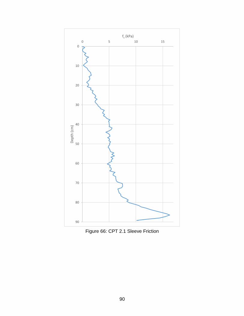
66. CPT 2.1 Sleeve Friction ..................................................................... 90
67. CPT 2.1 Friction Ratio ....................................................................... 91
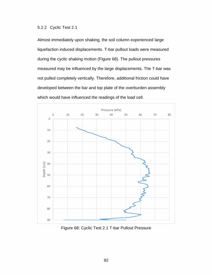
68. Cyclic Test 2.1 T-bar Pullout Pressure .............................................. 92
69. Cyclic Test 2.1 Excess Pore Pressures ............................................. 93
70. Displaced Bucket After Cyclic Test 2.1 .............................................. 94

xiii
71. CPT 2.2 Corrected Tip Resistance .................................................... 95
72. CPT 2.2 Sleeve Friction ..................................................................... 96
73. CPT 2.2 Friction Ratio ....................................................................... 97
74. Cyclic Test 2.2 T-bar Pullout Pressure .............................................. 99
75. CPT 2.3 Corrected Tip Resistance .................................................. 100
76. CPT 2.3 Sleeve Friction ................................................................... 101
77. CPT 2.3 Friction Ratio ..................................................................... 102
78. CPT Summary ................................................................................. 104
79. T-bar Pullout Pressure Summary .................................................... 106
80. T-bar Pullout Pressure Cyclic Tests 1.1 and 2.1 ............................ 107
81. Cyclic Test 2.1 Excess Pore Pressures ........................................... 108
82. Cyclic Test 2.1 Accelerations ........................................................... 109
83. Comparison of Excess Pore Pressures and Accelerations (Cyclic
Test 2.1) .......................................................................................... 111
84. Su Calculated from T-bar Pullout Test Summary ............................. 113
85. Comparison of Su Calculated from T-bar Pullout Test Cyclic Tests
1.1 and 2.1 ...................................................................................... 114
86. Cyclic Test 1.1 Liquefied Strength Ratio vs. Normalized CPT Tip
Resistance ....................................................................................... 115
87. Comparison of Cyclic Test 1.1 Results to Olson and Stark (2003) .. 116
88. Cyclic Test 2.1 Liquefied Strength Ratio vs. Normalized CPT Tip
Resistance ....................................................................................... 117
89. Comparison of Cyclic Test 2.1 Results to Olson and Stark (2003) .. 118

1
CHAPTER 1 LITERATURE REVIEW
1.1 Overview
In areas underlain by loose saturated granular materials, soil liquefaction
can be a major cause of damage in earthquake events. Soil liquefaction has
been an area of extensive research in geotechnical engineering for over 50
years. The phenomenon was thrust into the geotechnical engineering world
following two earthquakes in 1964: the Niigata, Japan and Great Alaskan
earthquakes. Both events resulted in damage caused by seismically
induced liquefaction (Seed et al., 2003). Seed et al. (2003) established a
flow chart of key elements of liquefaction engineering (Figure 1). The
research contained herein attempts to provide additional laboratory data for
step 2: assessment of post-liquefaction strength and overall post
liquefaction stability.

2
1.2 Seismically-induced liquefaction mechanics
Saturated contractive sands can experience a loss of shear strength when
subjected to rapid shearing strain. Rapid shearing causes the soil to
develop excess pore water pressures that can cause the soil to temporarily
behave as a viscous fluid, gradually regaining strength as the excess pore
water pressure dissipates. Typical effects of seismically-induced
liquefaction include: loss of bearing strength, lateral spreading, sand boils,
flow failures, ground oscillation, flotation of underground structures, and
settlement (NAE 2016).
Figure 1: Key Elements of Soil Liquefaction Engineering (Seed et al., 2003)

3
In past research, many terms have been used to describe the minimum
strength of a soil in the liquefied state: undrained steady-state strength
(Poulos et al., 1985), undrained residual shear strength (Seed, 1987),
undrained critical shear strength (Stark and Mesri, 1992), shear strength of
liquefied soils (Stark et al., 1998), liquefied shear strength (Olson and Stark,
2003), and residual strength (Dewoolkar et al., 2016).
This research will use the term residual strength (Sr) to represent the
minimum shear strength mobilized in the liquefied state.
1.3 Liquefaction Triggering
Engineers working with potentially liquefiable soils need to assess if
liquefaction will be triggered by the earthquake motions considered in their
design. The most widely used approach to assess potential for triggering
liquefaction is a stress-based approach that compares the earthquake-
induced cyclic stresses with the cyclic resistance of the soil (Youd et al.,
2001).
Seed and Idriss (1970) first compared the occurrence/non-occurrence of
liquefaction with in-situ properties of sands in order to predict liquefaction
based on in-situ tests (Figure 2).

4
Seed and Idriss (1971) further expanded on their previous research to
create liquefaction triggering curves based on Standard Penetration Test
(SPT) blow counts and cyclic stress ratio (CSR). CSR is the ratio of shear
stress to vertical effective stress. The SPT blow counts were recorded post-
liquefaction. CSRs were estimated using the peak ground acceleration
(PGA), duration of shaking, stress conditions of the liquefied layer, and a
non-linear shear stress participation factor (rd). The simplified equation
proposed by Seed and Idriss (1971) is:
𝐶𝑆𝑅 = 𝜏𝐴𝑉
𝜎0′= 0.65 ∗
𝑎𝑚𝑎𝑥
𝑔∗
𝜎0
𝜎0′∗ 𝑟𝑑
Figure 2: Evaluation of Liquefaction Potential for Fine Sands (Seed and Idriss, 1970)

5
Seed and Idriss (1971) plotted (N1)60 (SPT N values corrected for
overburden and hammer efficiency) vs CSR for a selection set of
earthquakes and marked whether or not the effects of liquefaction were
observed post-shaking (Figure 3).
Over the years, researchers have added to the suite of liquefaction
triggering data available in the triggering curves first presented by Seed and
Idriss (1970).
Researchers created new liquefaction triggering curves based on different
in-situ index tests, including CPT (Shibata and Teparaska, 1988; Seed and
De Alba, 1986; Mitchell and Tseng, 1990; Stark and Olson, 1995; Suzuki et
al., 1995; Robertson and Campanella, 1985; Robertson and Wride, 1998;
Toprak et al., 1999; Juang et al. 2002; Moss, 2003; Moss et al., 2006; Idriss
and Boulanger 2008).
An additional liquefaction triggering curve was developed using
overburden-corrected shear wave velocity (Vs) by Andrus and Stokoe
(2000) (Figure 4).
Researchers have also created probabilistic correlations for the potential of
triggering liquefaction to allow engineers to assess liquefaction triggering in
performance-based engineering analyses (Moss et al., 2006) (Cetin et al.,
2002) (Figure 5).

6
Figure 3: Relationship Between Stress Ratios Causing Liquefaction and N1-values for Clean Sands for M=7.5 Earthquakes (Seed and Idriss, 1971)

7
Figure 4: Vs Curves Recommended at Various Fines (Andrus and Stokoe, 2000)

8
Figure 5: Contours of Probability of Liquefaction (Moss et al., 2006)

9
1.4 Residual Strength Estimation
Static or dynamic loading of liquefiable soils can result in large permanent
deformations of soil. These large deformations occur when shear stresses,
dynamic or static, become larger than the available shear strength of the
soil. Evaluation of this critical shear strength, residual strength, that can be
mobilized by liquefiable soils is an important part of geotechnical
engineering practice. Two methods are utilized to estimate residual strength
of liquefiable soils: case history back-calculations and laboratory testing.
1.4.1 Case History
One method to estimate the residual strength of liquefied materials, is to
back-calculate strengths from case history events. Seed (1986) first
developed estimates for in-situ Sr of liquefied sand using this method. Earth
structures where liquefaction has occurred are modeled and analyzed to
estimate Sr of the suspected liquefied layers. Two main estimates of Sr are
evaluated using this method giving an upper and lower bound for residual
strength. The upper bound is the value of Sr that results in a sliding factor
of safety of 1.0 for the undeformed (pre-failure) geometry of the earth
structure. The other estimate of Sr is performed similarly, but for the post-
deformation geometry of the earth structure (Seed, 1986). This procedure
has been modified and the suite of failures analyzed has been expanded by
many researchers (Davis et al., 1988; Seed and Harder, 1990; Stark and

10
Mesri, 1992; Ishiharara, 1993; Wride et al., 1999; Yoshimine et al., 1999;
Olson and Stark, 2003; Kramer and Wang, 2015; Weber et al., 2015).
Researchers have interpreted this suite of back-calculated residual strength
estimates for comparison to in-situ tests in an attempt to allow engineers to
estimate Sr for projects with liquefiable layers. Initially, Sr was correlated
with equivalent clean sand SPT corrected blow count (N1,60cs) (Seed, 1987;
Seed and Harder, 1990). Recent researchers have expressed Sr as a
normalized liquefied shear strength ratio (Sr/σ’vc) (Vasquez-Herrera et al.,
1990; Stark and Mesri, 1992; Yoshimine et al., 1999; Olson and Stark, 2002;
Idriss and Boulanger, 2007).
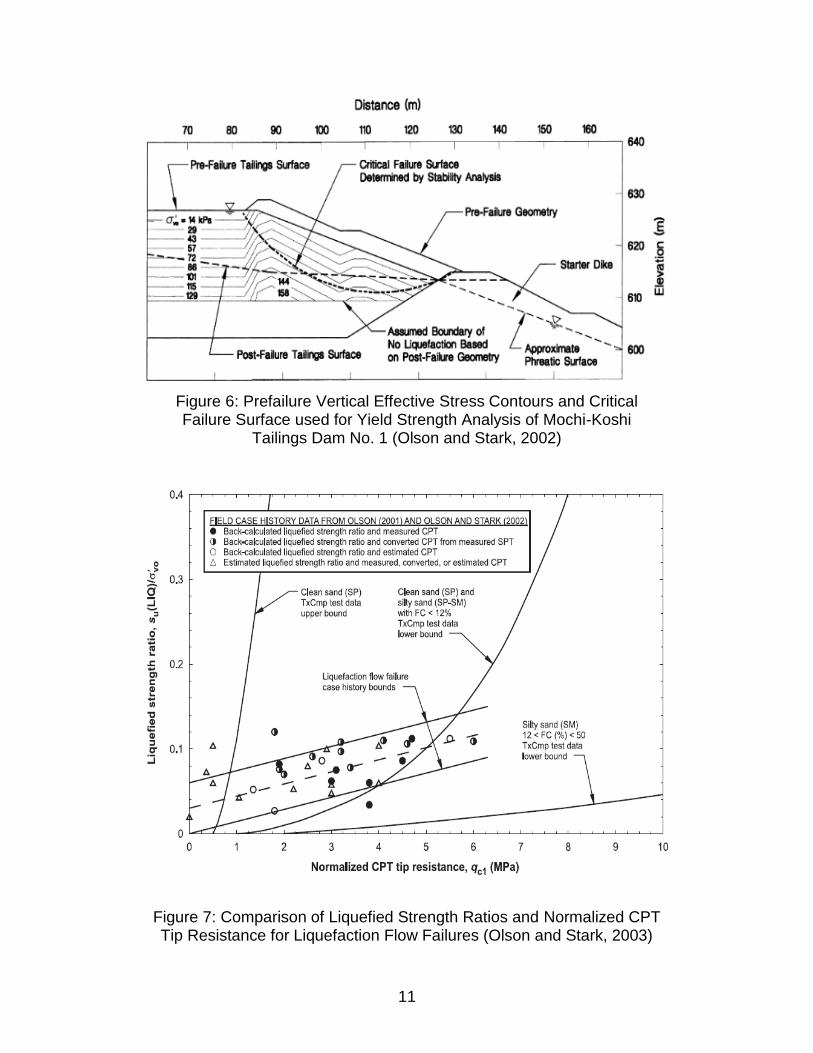
Olson and Stark (2002) estimated shear strength of liquefied soil by back-
calculating 33 cases of static liquefaction flow failure (Figure 6). They
proposed a linear relationship between yield shear strength and pre-failure
vertical effective stress. Olson and Stark (2003) correlated the yield strength
ratios to corrected SPT and CPT penetration resistance (Figure 7). These
correlations allow for an analysis of liquefaction susceptibility and an
estimation of yield strength ratio with the proposed relationships using
penetration resistance.
11
Figure 6: Prefailure Vertical Effective Stress Contours and Critical Failure Surface used for Yield Strength Analysis of Mochi-Koshi
Tailings Dam No. 1 (Olson and Stark, 2002)
Figure 7: Comparison of Liquefied Strength Ratios and Normalized CPT Tip Resistance for Liquefaction Flow Failures (Olson and Stark, 2003)

12
Kramer and Wang (2015) developed an alternative approach to the back-
analysis of flow slide case histories. The alternate procedure attempts to
characterize and account for uncertainties in the case histories, correct for
inertial effects, and evaluate the quality of each case. Using the results of
this alternate procedure, Kramer and Wang created a new model for
estimating the residual strength of liquefied soil. Included in this new model
are multiple forms of equations, direct and normalized, that relate residual
strength to SPT resistance while accounting for effective stress (Figure 8,
Figure 9).
Figure 8: Median Residual Strengths Predicted by Model (Kramer and Wang, 2015)

13
Weber et al. (2015) also developed new methods for the evaluation of in
situ liquefied strengths using full-scale liquefaction failure case histories.
Like Kramer and Wang (2015), Weber et al. (2015) used a suite of 30 back-
analyzed full-scale field liquefaction failures including inertial effects. This
research created new predictive strength relationships that reasonably
agree with previous recommendations over the lower ranges of effective
stress and penetration resistance for higher ranges. These relationships
were presented in a fully probabilistic form which could be used for risk
studies, but were also simplified to deterministic recommendations that
Figure 9: Predicted Variation of Residual Strength with Initial Vertical Effective Strength (Kramer and Wang, 2015)

14
could be applied to simpler analyses. Figure 10 shows a comparison
between the proposed relationships of Olson and Stark (2002) and Weber
et al. (2015).
1.4.2 Laboratory Testing
Laboratory tests used to estimate liquefied residual strength should be
performed under similar loading conditions to field conditions because the
measured shear resistance of the sample depends on consolidation
stresses and the loading direction (Idriss and Boulanger, 2008). Traditional
lab testing results in estimates of SCS (critical-state shear resistance) or
Figure 10: Comparison Between Olson and Stark (2002) and Weber et al. (2015)

15
SQSS (quasi steady state shear resistance) that correspond to the void ratio
of the sample when tested. Traditional laboratory testing is unable to
replicate void redistribution, particle intermixing, and other field
mechanisms that occur during earthquake motions. These mechanisms are
difficult for engineers to estimate and quantify their effect on strengths
measured in lab, making the results of these tests difficult to rely on in
design (Idriss and Boulanger, 2008).
De Alba and Ballestero (2006) measured residual shear strength of liquefied
sands using a sphere pulled through long triaxial specimens (Figure 11).
Their research studied the effect of loading rate and drainage conditions on
residual strength. De Alba and Ballestero found that liquefied sand behaves
like a Bingham plastic with a residual strength that depends on strain rate
up to a strain rate of about 100 % strain per second. The shear resistance
of the liquefied material above the transition shear strain rate (about 100 %
strain per second) tended to flatten out and not depend on strain rate. Their
research showed that below the transition strain rate, residual strength
remained proportional to initial effective stress. The dependency on strain
rate helps explain the large variability in residual strength values estimated
and back-calculated in previous studies.

16
DeWoolkar et al. (2016) measured the residual shear strength of liquefied
sands using a seismic geotechnical centrifuge model, where thin coupons
were pulled horizontally through sand models during shaking to estimate
residual strength. A plan and sectional view of the apparatus used can be
seen in Figure 12.
Figure 11: Static Liquefaction Test, 1. Sphere Displacement, 2. Apparent Drag, 3. Pore Pressure Ratio (de Alba and Ballestero, 2006)

17
Dewoolkar et al. (2016) observed a rapid decrease in the coupon force
when shaking was initiated and excess pore pressures developed,
indicating liquefaction (Figure 13). The researchers also observed that post-
liquefaction recovery of shear strength appears linearly related to the
recovered effective vertical stress as pore pressures dissipate.
When comparing results of the residual strength measured in the centrifuge
tests to the design curve established by Idriss and Boulanger (2008),
Dewoolkar et al. (2016) observed that the measured Sr values fell generally
Figure 12: Plan and Sectional View of Typical Centrifuge Test Model Configuration (Dewoolkar et al., 2016)

18
below the established design curve (Figure 14). The design curves’
overestimation of residual strengths shows the need for additional testing
and revisions to create design curves that can be trusted in practice.
Figure 13: Typical Coupon Force and Excess Pore Pressure Measurements from Centrifuge Tests (Dewoolkar et al., 2016)

19
Figure 14: Comparison of Measured Residual Strength and Residual Strength Ratios with SPT-based Correlations (Dewoolkar et al., 2016)
20
Dewoolkar et al. (2016) also measured residual strength using ring shear
tests. The ring shear specimens were prepared using a similar method to
the method used in the centrifuge models. A cyclic load with +/- 5% strain
of rotation was applied with the top ring to liquefy the sample. The samples
typically liquefied within two cycles. The ring shear tests measured residual
strength values within the same range as those observed in the centrifuge
tests. However, the residual strengths measured from the ring shear tests
did not follow the same pattern with changes in relative density as the
centrifuge tests and back-calculated estimates. Dewoolkar et al. (2016)
attributes the different trend observed in the ring shear testing to two factors:
ring shear does not capture the dilative soil response seen at higher relative
densities; and particle damage that occurs in the shear zone in the ring
shear tests.
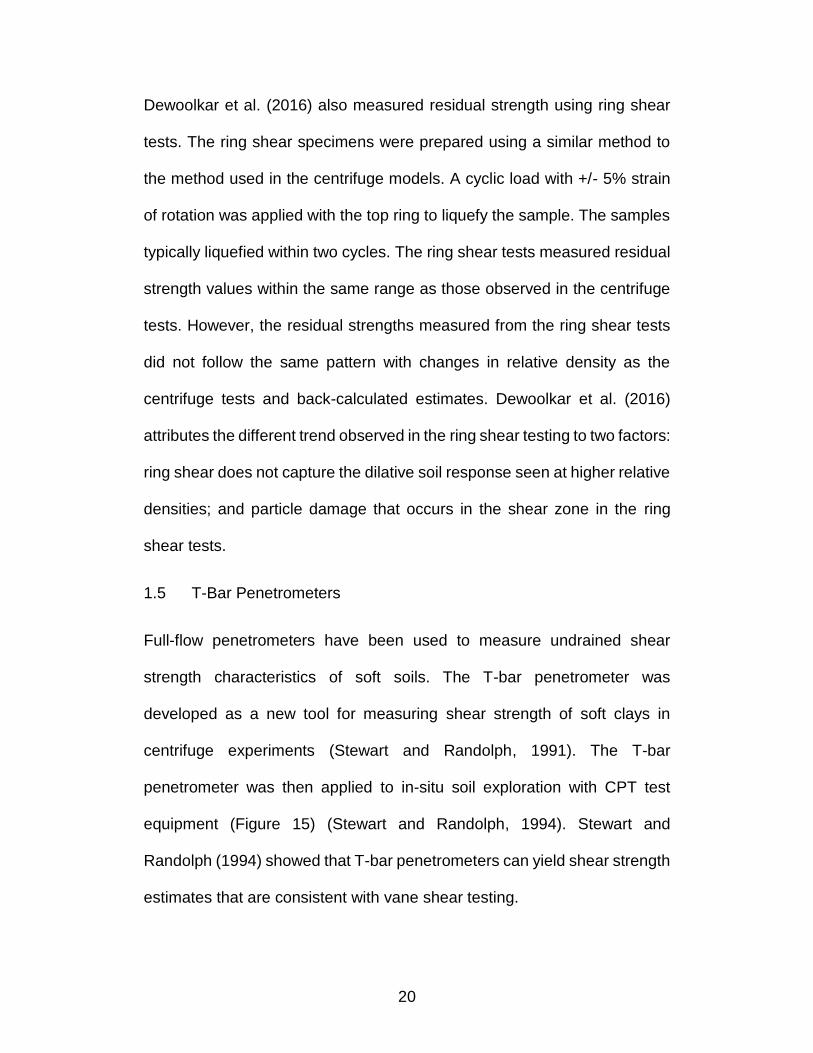
1.5 T-Bar Penetrometers
Full-flow penetrometers have been used to measure undrained shear
strength characteristics of soft soils. The T-bar penetrometer was
developed as a new tool for measuring shear strength of soft clays in
centrifuge experiments (Stewart and Randolph, 1991). The T-bar
penetrometer was then applied to in-situ soil exploration with CPT test
equipment (Figure 15) (Stewart and Randolph, 1994). Stewart and
Randolph (1994) showed that T-bar penetrometers can yield shear strength
estimates that are consistent with vane shear testing.

21
Figure 15: Field T-Bar Penetrometer (Stewart and Randolph, 1994)
Further testing using T-bar penetrometers has confirmed that the T-bar can
reliably estimate undrained shear strengths (DeJong et al., 2011). Their
ability to perform cyclic strength degradation testing and their increased
load cell sensitivity has seen an increase in their use with thick deposits of
soft clays, particularly offshore. See attached writeup in Appendix A.

22
1.6 Full-Scale Shake Table Testing
Towhata et al. (1999) performed a variety of 1-g shaking tests where the
drag force required to pull an embedded pipe laterally through the sample
was measured, similar to the centrifuge coupon drag tests described earlier
(Figure 16). Their research showed a much lower drag force was required
to pull the pipe through loose saturated sand than the force required to pull
the pipe through dry sand subjected to strong shaking. They also observed
the drag force to be rate dependent with the velocity of pipe movement,
suggesting a high value of apparent viscosity of liquefied sand.
Figure 16: Model Sand Container and Embedded Pipe (Towhata et al., 1999)

23
Motamed and Towhata (2010) performed a series of 1-g shake table tests
on a pile group and sheet-pile wall to observe the mechanisms of
liquefaction induced ground deformations and the behavior of a pile group
subjected to the large lateral displacements caused by liquefaction. They
studied the effects of several parameters on liquefied lateral displacement
including density, input motion amplitude and frequency, pile group head
fixity, and superstructure. The density of the sample was found to have a
significant effect on displacements because the development of excess
pore pressures proved to be highly dependent on initial density. Their
results showed that as the input motion’s amplitude increases, the lateral
deformations of the sample also increased; whereas, an increase in the
input motion’s frequency resulted in a decrease in lateral deformations
(Figure 17).

24
Figure 17: Time Histories of Surface Ground Displacement in Front of Pile Group (Motamad and Towhata, 2010)

25
CHAPTER 2 EQUIPMENT AND INSTRUMENTATION
Small-scale laboratory testing has been shown to not reliably capture void-
redistribution or the migration of excess pore pressure generation within a
sample (Idriss and Boulanger, 2008). In addition, small-scale laboratory
testing does not allow for full-scale CPT indexing to compare to in-situ field
exploration data. For these reasons, a large-scale testing procedure was
utilized herein in an attempt to capture these phenomena during testing.
2.1 Load Cell
A model SSC-500-0000 load cell manufactured by Tovey Engineering was
used to measure the load required to pull out the T-bar penetrometers
(Figure 18). The manufacturer's original calibration was input to LabVIEW
and then a more precise calibration was performed on October 18, 2016 to
correct for any variances from the manufacturer's original calibration. This
calibration was performed by loading the cell with known weights in 22.7 kg
increments ramped up to 229 kg and then ramped back down to zero in
22.7 kg increments. This revised calibration is saved to the LabVIEW
module in the Parsons Geotechnical and Earthquake Engineering
Laboratory.

26
Figure 18: Tovey Engineering SSC-500 Load Cell

27
2.2 Cone Penetrometer
Cone Penetration testing was utilized to monitor changes in soil stiffness
before and after shaking, and to allow for correlations between the lab
measurements and in-situ field data.
A 2.54 cm diameter instrumented piezometric cone penetrometer was
provided for testing by the Naval Facilities Engineering Command
(NAVFAC) (Figure 19). The cone penetrometer was mounted to a cross-bar
that held the 231 kg reaction mass required to drive the cone. The cross-
bar was mounted to the gantry crane in the Parsons Geotechnical and
Earthquake Engineering Laboratory which was used to raise and lower the
cone. The crane lowered the cone at a rate of 1.4 cm/s. ASTM D5778
suggests a descent rate of 2 cm/s for cone penetrometers; the gantry crane
in the has the capabilities for two speeds, 1.4 cm/s and 8.2 cm/sec. The
discrepancy between the speeds was not expected to cause appreciable
differences in the results of the cone penetrations.
The cone penetrometer used in this testing is capable of measuring tip load,
sleeve load, pore pressure, and displacement. The cone penetrometer uses
a DAQ system that is interfaced with a laptop to record four channels of
data (Figure 20).

28
Figure 19: NAVFAC Cone Penetrometer

29
2.3 T-bar Penetrometer
The T-bar penetrometers used herein have previously been used in
research by Crosariol (2010) and Kuo (2012). Both researchers used the T-
bar penetrometers in a soft clay exposed to cyclic motion. A bar factor of
10.5 was used to analyze the T-bar results in their studies (Moss and
Crosariol, 2013).
Figure 20: CPT Data Acquisition Interface

30
The T-bar penetrometers consist of a 95 mm long, 19 mm diameter steel
cylindrical cross bar welded to a 2.1 m long, 6.3 mm diameter steel rod
(Figure 21). An eyelet adapter was fabricated to thread onto the steel
pulling rod to allow for the load cell to be attached (Figure 22). Three
identical T-bar penetrometers were used throughout this research.
Figure 21: T-Bar Penetrometer (from Crosariol, 2010)

31
Figure 22: Eyelet Connector for T-Bar Penetrometer

32
2.4 Accelerometers
Ten PCB 393B04 Integrated Circuit Piezometer (ICP) accelerometers were
used to measure accelerations within the soil sample. These
accelerometers can measure accelerations up to +/-5 g’s. One PCB 353B52
ICP accelerometer was used to measure the accelerations of the shake
table. The manufacturer calibrations of these accelerometers are saved to
the DAQ system in the Parson’s Earthquake and Geotechnical Laboratory.
The accelerometers were connected to the DAQ system through a National
Instruments SCXI 1531 accelerometer amplifier. All accelerometers were
oriented to measure accelerations in the direction of shaking except for
accv1 and accv4, which were oriented to measure vertical accelerations.
The number attached to the accelerometer name refers to the instrument’s
location within the soil sample. The numbers increase as the sample is
ascended. Calibration values for these accelerometers are in Table 1. The
shake table control system has an additional accelerometer embedded
within the shake table to control the response.

33
Table 1: Accelerometer Calibration Values
Accelerometer Calibration
Value mV/g
acci1 1000
acci2 1000
acci3 988
acci4 1028
acct1 982
acct2 1020
acct3 1000
acct4 1028
accv1 1000
accv4 1000
acctable 502
2.5 Pore Pressure Transducers
Four Omega PX481A-015G5V stainless steel industrial pore pressure
transducers (PPTs) were used to measure excess pore-water pressures
generated during shaking. These gages require an excitation voltage of 10
volts and provide output voltages ranging from 0 volts to 5 volts that
correspond to a pressure range of 0 kPa to 103 kPa gage. The pore
pressure transducers follow a similar naming convention as the
accelerometers, with the suffix number increasing with ascending vertical
height in the sample. These pressure transducers were calibrated in

34
previous testing (Jacobs 2016) using a hydrostatic water column and an air
compressor. Calibration values for each pore pressure transducer are
presented in Table 2. The PPTs were interfaced with the DAQ system with
a National Instruments SCXI 1520 Universal Strain Gage input module.
Table 2: Pore Pressure Transducer Calibration Values
ppt 0 1 2 3
kPag Volts D.C.
0.7 0.82 0.79 0.81 0.81
13.8 1.34 1.31 1.33 1.33
34.5 2.15 2.13 2.15 2.14
68.9 3.50 3.47 3.49 3.49
103.4 4.85 4.82 4.84 4.84
Figure 23: Pore Pressure Transducer and Accelerometer Instrument Package (From Jacobs, 2016)

35
2.6 Tactile Pressure Sensors
Two PPS ConTacts C-500 Tactile Sensors were used to estimate the
overburden pressure applied to the soil sample. The sensors are set up in
waterproof jackets. Calibration values and plots were provided by the
manufacturer for each sensor. The sensors were placed above the sand
layer, between the landscape fabric the bottom plate of the overburden
assembly.
2.7 Backup overburden estimation
As a backup to the tactile pressure sensors. A flat scale was placed
between the inner tube and top plate of the overburden assembly. The force
on the scale was recorded to estimate the overburden pressure acting on
the bottom plate.
2.8 Displacement Transducers
Three ASM WS10SG Posiwire Cable Extension Position Sensors were
used to measure displacement of the outside of the flexible bucket
membrane. The sensors were mounted to the Kevlar bands at three
different heights above the table. Previous testing showed that other wire
potentiometers were incapable of accurately measuring displacements at 8
Hz (Jacobs, 2016). The sensors used in this research proved to be effective
at accurately measuring displacements at 8 Hz.

36
The sensors were calibrated by mounting the sensor body to a work table
and setting a grid of screws at 10 cm increments (Figure 24). The voltage
value of each sensor at every distance increment was recorded in LabVIEW
and calibration equations created that were input to the data acquisition
system.
2.9 Flexible Walled Testing Apparatus
This research used a 2.3 meter diameter by 1.5 meter tall flexible walled
testing apparatus (Figure 25). This apparatus consists of steel top and
bottom plates, and a 10 mm thick rubber membrane wall. The outer
diameter of the rubber was confined by 2.3 meter diameter Kevlar bands,
which are designed to act similar to the wire reinforced membranes used in
table top simple shear tests. The spacing of the bands varied with height
along the outside of the membrane. The bands were placed closer together
near the bottom of the membrane to better confine the higher pressures
present near the base.
Figure 24: Calibration of Cable Extension Position Sensors

37
Meymand (1998) investigated the effectiveness of the flexible walled bucket
used in this research in allowing free-field response. Meymand compared
soil accelerations recorded at various depths in a soft clay sample with
numerically simulated accelerations simulated by SHAKE 91. Figure 26
shows relative agreement between the tested (solid) and the computed
(dashed) 5% damped response spectra.
Figure 25: Flexible Walled Testing Apparatus

38
Figure 26: Site Response (solid) vs Predicted Response (dashed) Spectra (Meymand, 1998)

39
CHAPTER 3 PRE-TESTS
To familiarize use of the load cell, gantry crane, pluviation method, and the
data acquisition system, a series of pre-tests were completed using the
same or similar equipment to the main testing.
3.1 Dry Pluviated Trash Can Test
Monterey sand was dry pluviated into a 44-gallon container using the large
scale pluviation device described in Section 4.3. Three T-bar penetrometers
were embedded at the base of the sample spaced equidistant radially
around the center (Figure 27). The dry pluviation technique resulted in a
sample 59 cm tall with a dry unit weight of 16.8 kN/m3 relative density of
approximately 89%.
The three T-bar penetrometers were pulled out individually at a rate of 8.2
cm/sec, the faster speed of the gantry crane used for pullout. Figure 28
shows the average profile of the pullout pressure experienced by the three
T-bars.

40
Figure 27: Dry Pluviated 44 Gallon Test Sample

41
0
10
20
30
40
50
60
0 100 200 300 400 500 600 700 800 900 1000
Dep
th (
cm)
Pullout Pressure (kPa)
AVERAGE PRESSURE
- st dev
+ st dev
Figure 28: Average Dry Pluviated T-bar Pullout Pressure

42
Multiple CPT tests were performed on this dry pluviated sample. The first
CPT sounding was not perfectly vertical when the sounding began, causing
the penetrometer to drift. The second sounding was successful; however,
data were only obtained to a depth of 48 cm because the cone reached a
refusal depth where the driving force was not enough to continue pushing
the cone through the sample (Figures 29-31).

43
0
5
10
15
20
25
30
35
40
45
50
0 1000 2000 3000 4000 5000 6000 7000
Dep
th (
cm)
qc1 (kPa)
Figure 29: Dry Trash CPT 1.2 Corrected CPT Tip Resistance

44
0
5
10
15
20
25
30
35
40
45
50
0 2 4 6 8 10 12 14
Dep
th (
cm)
fs (kPa)
Figure 30: Dry Trash CPT 1.2 Sleeve Friction

45
0
5
10
15
20
25
30
35
40
45
50
0 0.2 0.4 0.6 0.8
Dep
th (
cm)
Rf (%)
Figure 31: Dry Trash CPT 1.2 Friction Ratio

46
3.2 Wet Pluviated Trash Can Test 1
Two additional test samples were created using a wet pluviation method.
These samples provided estimates for the relative density created using wet
pluviation, as well as provided a representative medium to test time-rate
effects of T-bar pullout.
Monterey sand was pluviated into a standing head of 5 to 15 cm of water
into a 44 gal container with three T-bars spaced equidistant at the bottom
(Figure 32). This wet pluviation method resulted in a sample with a dry unit
weight of 15.7 kN/m3 and a relative density of 45%. The T-bars were pulled
Figure 32: Wet Trash Can Specimen

47
at a rate of 8.2 cm/sec. The average of the three T-bar pullouts can be seen
in Figure 33.
A CPT sounding was performed in this sample. The cone was pushed at a
rate of 1.4 cm/s, the slower speed of the gantry crane used to lower the
cone penetrometer. The CPT cone was able to penetrate the full depth of
the specimen in this drive. The results of this sounding are shown in Figures
34-36.
0
10
20
30
40
50
60
0 50 100 150 200 250
Dep
th (
cm)
Pressure (kPa)
AVERAGE PRESSURE
- st dev
+ st dev
Figure 33: Average Wet Pluviated Trash 1 T-bar Pullout Pressure

48
0
10
20
30
40
50
60
70
80
0 200 400 600 800 1000 1200 1400
Dep
th (
cm)
qc1 (kPa)
Figure 34: Wet Trash CPT 1.1 Corrected CPT Tip Resistance

49
0
10
20
30
40
50
60
70
80
0.0 0.5 1.0 1.5 2.0 2.5 3.0
Dep
th (
cm)
fs (kPa)
Figure 35: Wet Trash CPT 1.1 Sleeve Friction

50
0
10
20
30
40
50
60
70
80
0.0 0.5 1.0 1.5 2.0 2.5
Dep
th (
cm)
Rf (%)
Figure 36: Wet Trash CPT 1.1 Friction Ratio
51
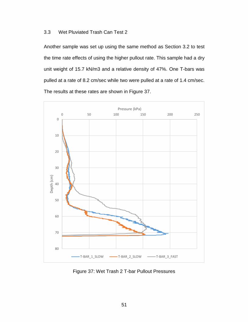
3.3 Wet Pluviated Trash Can Test 2
Another sample was set up using the same method as Section 3.2 to test
the time rate effects of using the higher pullout rate. This sample had a dry
unit weight of 15.7 kN/m3 and a relative density of 47%. One T-bars was
pulled at a rate of 8.2 cm/sec while two were pulled at a rate of 1.4 cm/sec.
The results at these rates are shown in Figure 37.
0
10
20
30
40
50
60
70
80
0 50 100 150 200 250
Dep
th (
cm)
Pressure (kPa)
T-BAR_1_SLOW T-BAR_2_SLOW T-BAR_3_FAST
Figure 37: Wet Trash 2 T-bar Pullout Pressures

52
As can be seen in Figure 37, time rate effects were observed for the T-bar
pullouts. The T-bars pulled at the faster rate (8.2 cm/sec) remained at a
higher pressure for approximately 30 cm before settling, while the T-bars
pulled at the slower rate (1.4 cm/sec) remained at a higher pressure for
approximately 15 cm before settling. However, the results, although
stretched, are comparable. Therefore, a pullout rate of 8.2 cm/sec was
determined to be appropriate to use for the full-scale shake table testing.
This higher rate is much better suited to this testing because the T-bars can
ascend the height of the sample in approximately 15 seconds, as opposed
to approximately 60 seconds if the slower pullout rate was used.
3.4 Shake Table Transfer Function
Prior to the clay and sand placement, the bucket was filled approximately
half-way with water to test the waterproofing and to estimate the transfer
function (Hinv) for the shake table control. This transfer function dictates
what the table control needs to send to the table in order to achieve a
desired output motion. The table was shaken with an 8 Hz, 0.5g, sine wave
with the water. The transfer function from this test was saved and used for
the full-scale sand tests. Originally, the transfer function from this pre-test
was designed to be used for the first test, with all subsequent tests using
the transfer function obtained from the previous test. However, after the first
cyclic test, the transfer function derived from the water-only was deemed to
be acceptable for all future tests.

53
Previously, a sine-sweep fast fourier transformation was performed on a
similar test configuration to that used in this research (Jacobs 2016). The
research found a first modal response of the soil column near 8 Hz (Figure
38). For this research, an 8 Hz sine wave was set to run for 122 cycles (15.3
seconds) to provide sufficient time to pull the T-bars through the liquefied
sample.
Figure 38: Sine Sweep Fast Fourier Transformation of the Uppermost Accelerometer (From Jacobs, 2016)

54
CHAPTER 4 MODEL PREPARATION
4.1 Bucket Waterproofing
Previous tests performed using the same flexible walled testing apparatus
were hindered due to imperfect waterproofing of the bucket. The steel base
of the apparatus was waterproofed using a combination of Titebond®
Weathermaster™ Metal Roof Sealant and an aerosol spray rubber coating.
The interface of the rubber wall and the steel base was waterproofed by
placing silicone between all interfaces at the bolt holes. This waterproofing
technique proved to be effective during testing, with no visible signs of
leakage.
Figure 39: Flexible Walled Testing Apparatus

55
4.2 Clay Placement
A 15 cm thick layer of soft clay was placed at the base of the flexible walled
testing apparatus. This clay layer helped ensure the apparatus was water
tight by providing an impermeable boundary between the saturated loose
sand and the base. The clay also allowed the appropriate height of the sand
layer to create a height to diameter ratio of 0.4 as specified in ASTM D6528
for simple shear testing.
The soft clay consisted of approximately 67.5% kaolonite, 22.5% betonite,
and 10% class C fly ash by mass of solids mixed at a water content of 125%.
This soft clay mixture has previously been vetted in studies by Crosariol
(2010), Kuo (2012), Noche (2013), Moss & Crosariol (2013), and Stanton
(2013). The clay mixture was mixed and pumped into the testing flexible
wall testing apparatus using an industrial grade Chem-Grout soil mixer. The
clay layer was separated from the saturated sand layer using semi-
permeable landscape fabric (Figure 40). The landscape fabric prevented
the fines from the clay from migrating into the saturated sand layer.

56
4.3 Sand Placement
The sand used in this testing is a #2/16 Monterey sand sourced from the
CEMEX Lapis Plant in Marina, California. Figure 41 shows an approximate
gradation of the #2/16 Monterey sand as reported by CEMEX quality control
(from Stanton, 2013). The sand created a 92 cm thick layer of granular
material above the soft clay. The sand layer was placed by dry pluviation
Figure 40: Clay Mixture and Filter Fabric at Base of Specimen

57
into a standing head of water ranging from 5 to 15 cm in depth. A large scale
pluviation device (Figure 42) was modeled after a No. 8 ASTM E-11 sieve
with a 2.36 mm aperture. The full device consisted of a large reservoir
hopper suspended above a metal screen constructed within a timber frame
with a 24” square opening. The metal screen of the pluviation device was
previously shown to produce samples with a 0.19% difference in total unit
weight when compared to a No. 8 ASTM E-11 sieve (Jacobs, 2016). The
large scale pluviation device was used to deposit the sand in the center of
the flexible walled testing apparatus while a No.8 ASTM E-11 sieve was
used to deposit the sand near the walls of the flexible walled testing
apparatus.
Figure 41: Approximate Grain Size Distribution of #2/16 Monterey Sand (Stanton 2013)

58
Figure 42: Large-Scale Pluviation Device

59
The maximum and minimum dry unit weights of the #2/16 Monterey Sand
were previously measured using the ASTM D4254-14 and D4253-14
procedures, respectively (Jacobs, 2016). The maximum and minimum dry
unit weights were calculated to be 17.1 and 14.7 kN/m3, respectively. These
results are in close agreement to previous studies performed by Hazirbaba
and Rathje (2009), Boulanger and Seed (1995), and Kammerer et al.
(2005), where the maximum dry unit weights of Monterey Sand ranged from
16.0-17.1 kN/m3, and minimum dry unit weights ranged from 13.1-13.9
kN/m3. During the sample placement, the mass of sand added was
recorded to determine an estimated dry unit weight of the sample. Assuming
the sand filled the volume of a rigid cylinder with a diameter of 230 cm and
a height of 92 cm, the dry unit weight of the sample is roughly 15.4 kN/m3,
resulting in a relative density (Dr) of approximately 32%.
Once the sand was deposited the full height of the sample (92 cm) (Figure
43), additional landscape fabric was placed down to protect the interface
between the top of the sand layer and the bottom of the overburden
assembly.

60
Figure 43: Top of Deposited Sand

61
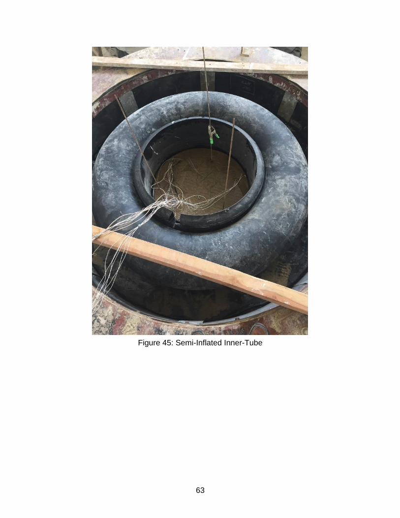
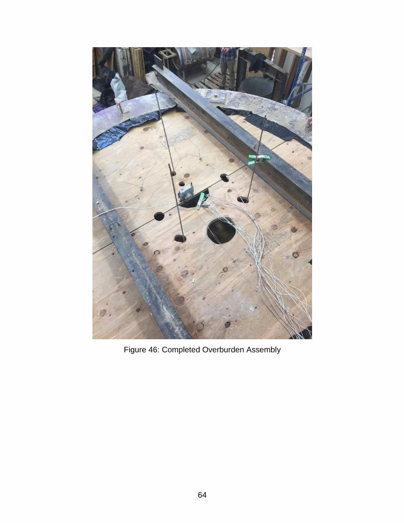
4.4 Overburden Assembly
Confinement of the soil sample was applied by inflating an 18.4/20.8R-42
inner tube within a confined area at the top of the flexible walled testing
apparatus. The inner tube was confined by 5/8” plywood at the bottom and
1-1/8” T&G plywood subfloor at the top protected by visqueen plastic. Two
W8x13 grade A992 rolled steel beams were attached to the upper rim of the
flexible walled testing container to provide the reaction force necessary on
the top plate to provide confinement of the inner tube. In order to prevent
the inner-tube from expanding into the space reserved for the T-bars and
CPT soundings, a 91 cm diameter high density polyethylene corrugated
drain pipe was placed in the annular space of the inner tube. The inner tube
was then inflated to apply an overburden pressure to the soil. The
overburden pressure was measured in two ways: PPS tactile pressure
sensors placed below the bottom plate of the overburden assembly, and a
flat scale placed between the inner tube and top-plate.

62
Figure 44: Bottom Plates of Overburden Assembly
63
Figure 45: Semi-Inflated Inner-Tube
64
Figure 46: Completed Overburden Assembly

65
4.5 Instrument Embedment
Two vertical arrays of instruments were embedded within the saturated
sand layer (Figure 47). Each array consisted of 4 instrument packages.
Each instrument package was mounted on an acrylic plate. The arrays used
anchored cables with crimped stoppers to rest at the proper height during
sand deposition and testing.
For each array, two 1.6 mm diameter cables were attached to the base of
the flexible walled testing apparatus using eyelets epoxy-bonded to the
base. The cable stoppers were spaced equidistant at a 20 cm spacing with
the bottom cable stop located 10 cm above the bottom of the saturated sand
layer. One array contained accelerometers oriented in the direction of
shaking motion with a vertical oriented accelerometer paired on the bottom
accelerometer. The second array contained accelerometers and pore
pressure transducers oriented in the direction of shaking motion. Both
arrays were spaced 30 cm forward (in the direction of shaking) of the center
of the bucket, with one array 25 cm to the left and the other array 25 cm to
the right. A schematic section and top view of the compelted bucket
assembly and instrument embendment can be seen in Figure 48 and Figure
49.

66
Figure 47: Accelerometer Embedment in Sand

67
Figure 48: Top View of Completed Specimen

68
Figure 49: Schematic Section of Completed Specimen

69
CHAPTER 5 TESTING
5.1.1 Pre-Liquefaction Shear Wave Velocity
Shear wave velocity of the soil sample was estimated using a procedure
similar to that outlined in Seismic Cone Downhole Procedure to Measure
Shear Wave Velocity (Butcher et al., 2005). A 46 cm long, 9 cm x 9 cm block
was placed at the top of the soil. Approximately 950 N were applied to the
block. The block was then struck with a rubber mallet on one side, and then
the other (Figure 50). The accelerometers were used to detect the shear
wave propagating through the soil profile. The first major cross-over of these
“butterflied” shear waves was used as the “reference” arrival of the shear
wave. Using accelerometers are different depths in the sample, the shear
wave velocity was estimated by taking the vertical distance between
accelerometers and dividing it by the difference in the time of reference
arrival.
The measured shear wave velocity of the sample is approximately 200
m/sec. Shear wave velocity was measured without the overburden
assembly, likely resulting in lower measured shear wave velocity than that
present during cyclic testing.

70
Figure 50: Shear Wave Velocity Testing

71
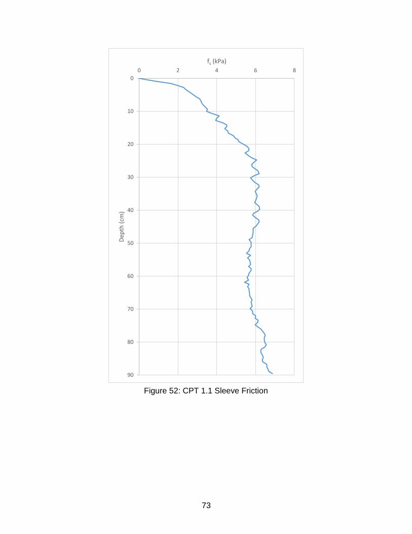
5.1.2 Initial Cone Penetration Test Sounding (CPT_1.1)
An initial CPT sounding was performed in the soil sample prior to the first
cyclic test. The cone penetrometer was pushed to a depth of 90 cm below
the soil surface. The overburden assembly provided a virtual overburden of
31.8 kPa during this sounding.

72
0
10
20
30
40
50
60
70
80
90
0 100 200 300 400
Dep
th (
cm)
qc1 (kPa)
Figure 51: CPT 1.1 Corrected Tip Resistance
73
0
10
20
30
40
50
60
70
80
90
0 2 4 6 8
Dep
th (
cm)
fs (kPa)
Figure 52: CPT 1.1 Sleeve Friction

74
0
10
20
30
40
50
60
70
80
90
0 2 4 6 8 10 12
Dep
th (
cm)
Rf (%)
Figure 53: CPT 1.1 Friction Ratio

75
5.1.3 Cyclic Test 1.1
A testing frequency of 8.0 Hz was run for 122 cycles (15.3 seconds). An
output from the table control during the shaking can be seen in Figure 54.
“Control” in the figure is the true table accelerations while “profile” is the
input motion. As can be seen in the figure, the transfer function used for this
setup created a response very similar to the input.
From visual observation, the sample liquefied almost instantaneously as
motion started. There was a failure with the DAQ system during this test
and many sensors did not record data during the motion. The DAQ system
did not record pore pressures, bucket displacement, and accelerations
during this test.
Figure 54: Shake Table Control Output

76
One T-bar was lifted during this cyclic test. The lifting began approximately
2 seconds after shaking began. The load required to lift the T bar was
measured at a rate of 600 Hz and a graph of the pressure on the T-bar vs.
Depth can be seen in Figure 55.
After the shaking was finished, 18 cm of saturated sand ejecta and an
additional 21.5 cm of water filled the annular space of the bucket top. The
overburden pressure dropped 8.4 kPa to 23.4 kPa.
0
10
20
30
40
50
60
70
80
90
0 5 10 15 20 25 30 35
Dep
th (
cm)
Pressure (kPa)
Figure 55: Cyclic Test 1.1 T-bar Pullout Pressure

77
The bucket displaced laterally during the first cyclic test that resulted in a
pure shear strain of 16.1% (Figure 56). The bucket was tied off to an anchor
to resist any further deformations in the direction perpendicular to the
shaking motions.
Figure 56: Displaced Bucket After Cyclic Test 1.1

78
5.1.4 CPT_1.2
A CPT sounding was performed after the first cyclic test to categorize any
change in soil stiffness and structure. The cone was pushed to a depth of
64 cm before initial refusal. An additional 95 kg of driving mass was added
to the cone penetrometer which drove the cone to a depth of 73 cm before
reaching refusal.

79
0
10
20
30
40
50
60
70
80
90
0 1000 2000 3000 4000
Dep
th (
cm)
qc1 (kPa)
Figure 57: CPT 1.2 Corrected Tip Resistance

80
-2 0 2 4 6 8 10
fs (kPa)
Figure 58: CPT 1.2 Sleeve Friction

81
0 1 2 3 4 5 6
Rf (%)
Figure 59: CPT 1.2 Friction Ratio

82
5.1.5 Cyclic Test 1.2
A second cyclic test was run at the same parameters as Cyclic Test 1 with
approximately 23.4 kPa of effective overburden. The DAQ system failed to
record displacements and the load cell measurements for this test. Excess
pore pressures were successfully recorded during this test. Excess pore
pressures rose immediately upon shaking, but never reached an excess
pore pressure ratio of 1.0. The excess pore pressures generated during
shaking can be seen in Figure 60.
.

83
-1
-0.5
0
0.5
1
1.5
2
0 5 10 15 20 25
Exce
ss P
ore
Pre
ssu
re (
kPa)
Time (sec)
75 per. Mov. Avg. (ppt3)
75 per. Mov. Avg. (ppt2)
75 per. Mov. Avg. (ppt1)
75 per. Mov. Avg. (ppt0)
Figure 60: Cyclic Test 1.2 Excess Pore Pressures

84
5.1.6 Cyclic Test 1.3
A third cyclic test was performed with the same parameters as the previous
two. The T-bar pullout pressure can be seen in Figure 61. After shaking
finished, the overburden pressure dropped to approximately 22.6 kPa.
0
10
20
30
40
50
60
70
80
90
0 200 400 600 800 1000 1200
Dep
th (
cm)
Pressure (kPa)
Figure 61: Cyclic Test 1.3 T-Bar Pullout Pressure

85
5.1.7 CPT_1.3
A CPT sounding was performed after the third cyclic test. The cone was
pushed with an additional 95 kg of driving mass to a depth of 63 cm before
refusal.
0
10
20
30
40
50
60
70
80
90
0 500 1000 1500 2000 2500
Dep
th (
cm)
qt (kPa)
Figure 62: CPT 1.3 Corrected Tip Resistance

86
0
10
20
30
40
50
60
70
80
90
0 2 4 6 8 10 12
Dep
th (
cm)
fs (kPa)
Figure 63: CPT 1.3 Sleeve Friction

87
0
10
20
30
40
50
60
70
80
90
0 1 2 3 4 5
Dep
th (
cm)
Rf (%)
Figure 64: CPT 1.3 Friction Ratio

88
5.2 Setup 2
After the first round of cyclic testing, the sand was removed from the
specimen and was placed into sunlight to reduce the moisture content. The
sand was then redeposited into the flexible walled testing apparatus
following the method described in Chapter 4. The resulting soil column had
a relative density of approximately 34.6% and a shear wave velocity of
approximately 200 m/sec. The overburden assembly was pressurized to an
approximate overburden pressure of 27.6 kPa.
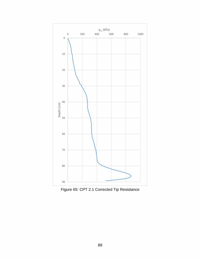
5.2.1 CPT_2.1
An initial pre-liquefaction CPT sounding was performed on the second
specimen. The CPT cone was driven a depth of 90 cm.
89
0
10
20
30
40
50
60
70
80
90
0 200 400 600 800 1000
Dep
th (
cm)
qc1 (kPa)
Figure 65: CPT 2.1 Corrected Tip Resistance
90
0
10
20
30
40
50
60
70
80
90
0 5 10 15
Dep
th (
cm)
fs (kPa)
Figure 66: CPT 2.1 Sleeve Friction

91
0
10
20
30
40
50
60
70
80
90
0 1 2 3 4 5 6
Dep
th (
cm)
Rf (%)
Figure 67: CPT 2.1 Friction Ratio
92
5.2.2 Cyclic Test 2.1
Almost immediately upon shaking, the soil column experienced large
liquefaction induced displacements. T-bar pullout loads were measured
during the cyclic shaking motion (Figure 68). The pullout pressures
measured may be influenced by the large displacements. The T-bar was
not pulled completely vertically. Therefore, additional friction could have
developed between the bar and top plate of the overburden assembly
which would have influenced the readings of the load cell.
0
10
20
30
40
50
60
70
80
90
0 10 20 30 40 50 60 70 80
Dep
th (
cm)
Pressure (kPa)
Figure 68: Cyclic Test 2.1 T-bar Pullout Pressure

93
The excess pore pressures recorded by the transducers can be seen in
Figure 69. Upon completion of the shaking, the soil column experienced a
pure shear strain of roughly 41% (Figure 70).
0
1
2
3
4
5
6
7
8
9
10
0 5 10 15 20 25
Exce
ss P
ore
Pre
ssu
re (
kPa)
Time (sec)
75 per. Mov. Avg. (ppt0)
75 per. Mov. Avg. (ppt1)
75 per. Mov. Avg. (ppt2)
75 per. Mov. Avg. (ppt3)
Figure 69: Cyclic Test 2.1 Excess Pore Pressures

94
Figure 70: Displaced Bucket After Cyclic Test 2.1

95
5.2.3 CPT_2.2
A post-liquefaction CPT sounding was performed on the sample. The CPT
cone was driven a depth of 72 cm before refusal.
0
10
20
30
40
50
60
70
80
90
0 200 400 600 800 1000 1200D
epth
(cm
)qc1 (kPa)
Figure 71: CPT 2.2 Corrected Tip Resistance

96
0
10
20
30
40
50
60
70
80
90
0 2 4 6 8 10
Dep
th (
cm)
fs (kPa)
Figure 72: CPT 2.2 Sleeve Friction

97
0
10
20
30
40
50
60
70
80
90
0 1 2 3 4 5 6
Dep
th (
cm)
Rf (%)
Figure 73: CPT 2.2 Friction Ratio

98
5.2.4 Cyclic Test 2.2
Prior to cyclic test 2.2, the bucket was tied off to an anchor to prevent
further lateral deformations perpendicular to the shaking motion. A T-bar
pullout was performed during the cyclic shaking (Figure 74). Similar to
cyclic test 2.1, the results of this pullout test may be influenced by a
pullout angle that was not vertical, and potential friction between the T-bar
rod and top plate of the overburden assembly. The T-bar was pulled
approximately 50 cm, to a final depth of 40 cm, during the test. The
sample laterally displaced such that the rubber membrane came in contact
with one of the vertical supports of the top ring of the assembly. The
membrane became sandwiched between this support and the bottom
plate of the overburden assembly, causing a separation to develop in the
membrane. This separation prevented any further testing because water
and sand began pouring out of the separation.

99
0
10
20
30
40
50
60
70
80
90
100
0 50 100 150 200 250
Dep
th (
cm)
Pullout Pressure (kPa)
Figure 74: Cyclic Test 2.2 T-bar Pullout Pressure

100
5.2.5 CPT_2.3
A final CPT push was performed in the sample after Cyclic Test 2.2. This
CPT was driven to a depth of 66 cm before refusal.
0
10
20
30
40
50
60
70
80
90
0 500 1000 1500 2000
Dep
th (
cm)
qc1 (kPa)
Figure 75: CPT 2.3 Corrected Tip Resistance

101
0
10
20
30
40
50
60
70
80
90
0 5 10 15 20 25
Axi
s Ti
tle
fs (kPa)
Figure 76: CPT 2.3 Sleeve Friction

102
0
10
20
30
40
50
60
70
80
90
0 1 2 3 4 5 6
Axi
s Ti
tle
Rf (%)
Figure 77: CPT 2.3 Friction Ratio

103
CHAPTER 6 RESULTS
This chapter presents analysis and results of the data presented in the
previous chapter. A summary of the data recorded by the data acquisition
system is presented. Summaries of the CPT and T-bar results are shown.
Observation of excess pore water pressure gives insight into pore pressure
dissipation is shown. A discussion of the liquefied soils response to the input
motion is provided. Estimates of liquefied residual strength are calculated
and compared to previous correlations with index tests.
6.1 Data Acquisition
As described in the previous section, the data acquisition system failed to
record all sensors during the testing. Table 3 shows which channels of the
data acquisition were stored for each test.
Test acci1 acci2 acci3 acci4 acct1 acct2 acct3 acct4 accv1 accv4 atab DTG1 DTG2 DTG3 PPT0 PPT1 PPT2 PPT3 LC7
1.1 X X X X X X1.2 X X X X X X X X X X X X1.3 X X X X X X X X X X X X X X X X2.1 X X X X X X X X X X X X X X X X X2.2 X X X X X X X X X X X X X
X Data Recorded Data Malfunction
Table 3: Data Acquisition Summary

104
6.2 CPT Summary
A summary of the normalized tip resistance (qc1) of all CPT tests performed
on the full-scale specimen can be seen in Figure 78.
0
10
20
30
40
50
60
70
80
90
0 1000 2000 3000 4000 5000
Dep
th (
cm)
qc1 (kPa)
1.1
1.2
1.3
2.1
2.2
2.3
Figure 78:CPT Summary

105
The CPT comparisons show that the specimen created for both sets of
testing were similar in properties before shaking, with the specimen created
before the second set of testing being slightly denser than the first. As
expected, CPT Tip Resistance at depth increased with each successive
test, showing that void redistribution had occurred. Presumably, void
redistribution caused the deeper section of the sand matrix to densify as
pore pressures dissipated.
6.3 T-Bar Penetrometer Summary
A summary of the pullout pressure calculated from the T-bar pullout tests
recorded can be seen in Figures 79 and 80. Similar to the CPT summary,
The T-bar pullout pressures at depth increased with each successive test.
This increase in pullout pressure is caused by the densification of soil post-
liquefaction.

106
0
10
20
30
40
50
60
70
80
90
0 200 400 600 800 1000 1200
Dep
th (
cm)
Pullout Pressure (kPa)
1.1 1.3 2.1 2.2
Figure 79: T-bar Pullout Pressure Summary

107
0
10
20
30
40
50
60
70
80
90
0 10 20 30 40 50 60 70 80
Dep
th (
cm)
Pullout Pressure (kPa)
1.1 2.1
Figure 80: T-bar Pullout Pressure Cyclic Tests 1.1 and 2.1

108
6.4 Pore Pressure Dissipation
Excess pore pressures developed immediately upon shaking. Figure 81
(Cyclic Test 2.1) shows that pore pressure dissipation began at the bottom
of the sample and propagated upwards. Excess pore pressures in the
bottom sensor (ppt0) began to dissipate almost immediately after
developing.
0
1
2
3
4
5
6
7
8
9
10
0 5 10 15 20 25
Exce
ss P
ore
Pre
ssu
re (
kPa)
Time (sec)
75 per. Mov. Avg. (ppt0)
75 per. Mov. Avg. (ppt1)
75 per. Mov. Avg. (ppt2)
75 per. Mov. Avg. (ppt3)
Figure 81: Cyclic Test 2.1 Excess Pore Pressures

109
6.5 Liquefied Soil Effects on Motion
Law et al. (1997) showed that high frequency components of earthquake
motions can be filtered out by liquefied soils. They showed that liquefied
soils can greatly reduce the seismic energy of the input motion transmitted
to the ground surface.
A summary of selected accelerations recorded during Cyclic Test 2.1 can
be seen in Figure 82. The recorded accelerations began lower than the
input motion. Then, as shaking continued, accelerations of the sand
specimen began to increase from the bottom of the specimen upwards.
-2
-1.5
-1
-0.5
0
0.5
1
1.5
2
0 2 4 6 8 10 12 14 16
Acc
eler
atio
n (
g)
Time (sec)
acctable acci2 acci3 acci4
Figure 82: Cyclic Test 2.1 Accelerations

110
The liquefied soil’s reduced shear modulus reduced the energy transmitted
through the soil fabric. Then as shaking continued and void redistribution
occurred, the accelerations of the sand specimen grow higher than the input
motion. This is likely caused by the increase in shear modulus that occurs
with void redistribution. The cyclic cycle of this test did not continue long
enough for the accelerations to reach a steady state. A comparison of the
excess pore pressures generated and accelerations during Cyclic Test 2.1
can be seen in Figure 83.

111
-2
-1
0
1
2
3
4
5
6
7
8
-2
-1
0
1
2
3
4
5
6
7
8
0 5 10 15 20
Acc
eler
atio
n (
g)
Exce
ss P
ore
Pre
ssu
re (
kPa)
Time (sec)
acci2 acci3 acci4
75 per. Mov. Avg. (ppt1) 75 per. Mov. Avg. (ppt2) 75 per. Mov. Avg. (ppt3)
Figure 83: Comparison of Excess Pore Pressures and Accelerations (Cyclic Test 2.1)

112
6.6 Liquefied Residual Strength Estimation
Randolph and Houlsby (1984) developed closed-form solutions, using
classical plasticity theory, for the limiting pressure acting on a circular pile
moving laterally through soil. Meymand (1998) further expanded on their
research and developed the flowing equation:
𝑆𝑢 =𝑃
𝑁𝑏 ∗ 𝐷
Where Su is undrained shear strength; P is force per unit length acting on
the cylinder; Nb is bar factor; and D is diameter of the cylinder. A bar factor
(Nb) of 10.5 is used in this research as suggested by Randolph and Houlsby
(1984).

113
0
10
20
30
40
50
60
70
80
90
0 10 20 30 40 50 60 70 80 90 100
Dep
th (
cm)
Su (kPa)
1.1 1.3 2.1 2.2
Figure 84: Su Calculated from T-bar Pullout Test Summary

114
Figure 85: Comparison of Su Calculated from T-bar Pullout Test Cyclic Tests 1.1 and 2.1
0
10
20
30
40
50
60
70
80
90
0 1 2 3 4 5 6 7
Dep
th (
cm)
Su (kPa)
1.1 2.1

115
6.1.1 Cyclic Test 1.1
The liquefied strength ratio from Cyclic Test 1.1 was calculated by dividing
the Su estimated from the T-bar pullout by the vertical effective stress. A
graph of the liquefied strength ratio and normalized CPT tip resistance, qc1,
can be seen in Figure 86.
0
0.01
0.02
0.03
0.04
0.05
0.06
0.07
0.08
0.09
0.1
0 0.05 0.1 0.15 0.2 0.25 0.3 0.35 0.4
Liq
uef
ied
str
en
gth
rat
io, s
u(L
IQ)/σ
' vo
Normalized CPT tip resistance qc1 (MPa)
Figure 86: Cyclic Test 1.1 Liquefied Strength Ratio vs. Normalized CPT Tip Resistance

116
A comparison of the results of Cyclic Test 1.1 to Olson and Stark (2003)
can be seen in Figure 87.
Figure 87: Comparison of Cyclic Test 1.1 Results to Olson and Stark (2003)

117
6.1.2 Cyclic Test 2.1
As discussed previously, the Residual Strength (Su) calculated from the T-
bar pullout during Cyclic Test 2.1 could have been influenced by additional
friction between the T-bar and top plate of the flexible-walled testing
apparatus. This increase in friction would overestimate the liquefied
strength ratio for this test. The liquefied strength ratio from Cyclic Test 2.1
was calculated by dividing the Su estimated from the T-bar pullout by the
vertical effective stress. A graph of the liquefied strength ratio and
normalized CPT tip resistance, qc1, can be seen in Figure 88.
0
0.05
0.1
0.15
0.2
0.25
0 0.05 0.1 0.15 0.2 0.25 0.3 0.35 0.4 0.45
Liq
uef
ied
str
engt
h r
atio
, su(L
IQ)/σ
' vo
Normalized CPT tip resistance qc1 (MPa)
Figure 88: Cyclic Test 2.1 Liquefied Strength Ratio vs. Normalized CPT Tip Resistance

118
A comparison of the results of Cyclic Test 2.1 to Olson and Stark (2003)
can be seen in Figure 89.
Figure 89: Comparison of Cyclic Test 2.1 Results to Olson and Stark (2003)

119
CHAPTER 7 CONCLUSIONS AND RECOMMENDATIONS FOR
FUTURE RESEARCH
The full-scale cyclic simple shear tests and index testing performed in this
study provide a progression in both laboratory and field testing for
liquefaction. CPT index test data provided pre- and post- liquefaction index
data for comparison to field tests and allowed for observation of the effect
repeated liquefaction has on sand. T-bar penetrometer pullout tests
provided estimates of liquefied residual strength during cyclic testing. Pore
pressure recordings were used to directly observe the occurrence of
liquefaction and show the dissipation of excess pore pressures as void
redistribution occurs. Acceleration time-histories were used to show
liquefaction’s effect on how seismic energy propagates through soil layers.
7.1 Data Acquisition
The data acquisition system in the Parsons Geotechnical Laboratory
experienced many issues and failures throughout this research. A more
reliable system that could record all channels of input data at higher
frequencies would greatly enhance and refine the data obtained in future
research.

120
7.2 Overburden Measurement
The development of an accurate measurement of the overburden
assembly’s effect on effective stress would allow for more accurate
corrected CPT Tip Resistance (qc1) and normalized residual strength
estimations.
7.3 Shear-Wave Velocity Measurement
An efficient method of testing shear wave velocity while the overburden
pressure assembly is installed and pressurized would improve the results
of this research. The measurements of Vs between each test would allow
for additional comparisons to field index test data.
7.4 Flexible walled testing container
At the completion of testing, the rubber membrane of the flexible walled
testing apparatus was destroyed beyond repair and disposed of. For future
testing, a similar membrane with additional lateral stiffness may be
beneficial. Additional lateral stiffness would increase resistance to the
lateral deformations observed in this research. However, careful
consideration of the effects an increased boundary stiffness would have on
the sand specimen and its seismic response.

121
REFERENCES
Andrus, R.D., Stokoe, K.H., (2000). Liquefaction Resistance of Soils from
Shear-Wave Velocity. J. Geotech. Geoenvion. Eng., 126(11), 1015-
1025.
ASTM D4253 – 14: Standard Test Methods for Maximum Index Density
and Unit Weight of Soils Using a Vibratory Table. (2014, December
15), West Conshohocken, Pa: ASTM International.
ASTM D4254 – 14: Standard Test Methods for Minimum Index Density
and Unit Weight of Soils and Calculation of Relative Density. (2014,
December 15), West Conshohocken, Pa: ASTM International.
ASTM D5778 – 12: Standard Test Method for Electronic Friction Cone and
Piezocone Penetration Testing of Soils. (2012, January 1), West
Conshohocken, Pa: ASTM International.
Boulanger, R.W., and Seed, R.B., (1995). Liquefaction of sand under bi-
directional monotonic and cyclic loading. Journal of Geotechnical
Engineering, ASCE, 121(12), 870-878.
Butcher, A.P., Campanella, R.G., Kaynia, A.M., Massarsch, K.R., (2005).
Seismic Cone Downhole Procedure to Measure Shear Wave
Velocity – A Guide Prepared by ISSMGE TC10: Geophysical Testing
in Geotechnical Engineering. London: International Society for Soil
Mechanics and Geotechnical Engineering.
Cetin, K.O., Der Kiureghian, A., and Seed, R.B., (2002). Probabilistic
Models for the Initiation of Seismic Soil Liquefaction. Structural
Safety, 24, pp. 67-82.

122
Crosariol, V. A. (2010). Scale Model Shake Table Testing of Underground
Structures in Soft Clay. San Luis Obispo, Ca: Cal Poly Digital
Commons.
Davis, A. P., Jr., Poulos, S. J., and Castro, G., (1988). Strengths back
figured from liquefaction case histories. 2nd Int. Conf. on Case
Histories in Geotechnical Engineering, St. Louis, MO, 1693–1701.
Davis, A.P., Jr., Poulos, S.J., and Castro, G., (1988), Strengths Back
Figured from Liquefaction Case Histories. 2nd Int. Conf. on Case
Histories in Geotechnical Engineering, St. Louis, MO, 1693-1701.
de Alba, P., and Ballestero, T. P., (2006). Residual strength after
liquefaction: A rheological approach. Soil Dyn. Earthquake Eng.,
26(2–4), 143–151.
DeJong, J.T., Yafrate, N.J., DeGroot, D.J., (2011). Evaluation of Undrained
Shear Strength Using Full-Flow Penetrometers. J. Geotech.
Geoenviron. Eng., 137(1), 14-26.
Dewoolkar, M., Hargy, J., Anderson, I., de Alba, P., Olson, S.M., (2016).
Residual and Postliquefaction Strength of a Liquefiable Sand. J.
Geotech. Geoenviron. Eng., 2016, 142(2).
Hazirbaba, K., and Rathje, E.M., (2009). Pore Pressure Generation of Silty
Sands due to Induced Cyclic Shear Strains, Journal of Geotechnical
and Environmental Engineering, ASCE, 135(12), 1892-1905.
Idriss, I. M., and Boulanger, R. W., (2007). SPT- and CPT-based
relationships for the residual shear strength of liquefied soils.
Earthquake Geotechnical Engineering, 4th Int. Conf. on Earthquake
Geotechnical Engineering—Invited Lectures, K. D. Pitilakis, ed.,
Springer, Netherlands, 1–22.
123
Idriss, I. M., and Boulanger, R. W., (2008). Soil liquefaction during
earthquakes. Earthquake Engineering Research Institute, Oakland,
CA.
Ishihara, K., (1993). Liquefaction and flow failure during earthquakes.
Geotechnique, 43(3), 351-415.
Jacobs, J.S., (2016). Full-Scale Shake Table Cyclic Simple Shear Testing
of Liquefiable Soil. San Luis Obispo, Ca: Cal Poly Digital Commons.
Juang, C.H., Jiang, T., and Andrus, R.D., (2002). Assessing probability-
based methods for liquefaction potential evaluation. Journal of
Geotechnical and Geoenvironmental Engineering, 128(7): 580-589.
Kammerer, A.M., Pestana, J.M., and Seed, R.B., (2005). Behavior of
Monterey 0/30 Sand Under Multidirectional Loading Conditions.
Geomechanics, 154-173.
Kramer, S.L., Wang, C.H., (2015). Empirical Model for Estimation of the
Residual Strength of Liquefied Soil. J. Geotech. Geoenviron. Eng.,
2015, 141(9), 04015038.
Kuo, S., (2012). Scale Model Shake Table Testing of Shallow Embedded
Foundations in Soft Clay. San Luis Obispo, Ca, Cal Poly Digital
Commons.
Law, K.T., Song, Q., Fukue, M., (1997). Effects of Liquefaction on Seismic
Ground Motion. In Proceedings of the International Conference on
Soil Mechanics and Foundation Engineering, Hamburg, Germany,
695-698.
Meymand, P., (1998). Shaking table scale model tests of nonlinear soil-pile
superstructure interaction in soft clay. Ph.D. Disseration, University
of California, Berkeley.

124
Mitchell, J. K., and Tseng, D. J., (1990). Assessment of liquefaction
potential by cone penetration resistance. Proc., H. Bolton Seed
Memorial Symp. Duncan, J. M. BiTech, Vancouver, Canada, 335–
350.
Moss, R. E. S., Seed, R. B., Kayen, R. E., Stewart, J. P., Kiureghian, A. D.,
and Cetin, K. O., (2006). CPT-based probabilistic and deterministic
assessment of in situ seismic soil liquefaction potential. J. Geotech.
Geoenviron. Eng., 132(8), 1032–1051.
Moss, R.E.S., and Crosariol, V.A. (2013). Scale Model Shake Table Testing
of an Underground Tunnel Cross Section in Soft Clay. Earthquake
Spectra: November 2013, Vol. 29, No. 4, 1413-1440.
Moss, R.E.S., (2003). CPT-Based Probabilistic Assessment of Seismic Soil
Liquefaction Initiation. Ph.D. thesis, University of California at
Berkeley.
Motamed, R., and Towhata, I., (2010). Shaking Table Model Tests on Pile
Groups behind Quay Walls Subjected to Lateral Spreading. J.
Geotech. Geoenviron. Eng., 2010, 136(3), 477-489.
National Academies of Sciences, Engineering, and Medicine. (NAE).
(2016). State of the Art and Practice in the Assessment of
Earthquake-Induced Soil Liquefaction and Its Consequences.
Washington, DC: The National Academies Press.
Noche, R., (2013). Scale Model Shake Table Testing of Seismic Earth
Pressures in Soft Clay. San Luis Obispo, Ca: Cal Poly Digital
Commons.
Olson, S. M., and Stark, T. D., (2002). Liquefied strength ratio from
liquefaction flow failure case histories. Can. Geotech. J., 39(3), 629–
647.

125
Olson, S. M., and Stark, T. D., (2003). Use of laboratory data to confirm
yield and liquefied strength ratio concepts. Can. Geotech. J., 40(6),
1164–1184.
Poulos, S.J., Castro, G., and France, J.W., (1985). Liquefaction evaluation
procedure. J. Geotechnical Eng., ASCE 111(6), 772-91.
Randolph, M.F. and Houlsby, G.T., (1984). The limiting pressure on a
circular pile loaded laterally in cohesive soil. Geotechnique, 34(4),
613-623.
Robertson, P. K., and Campanella, R. G., (1985). Liquefaction potential of
sand using the CPT. J. Geotech. Eng., 111(3), 384–403.
Robertson, P.K., and Wride, C.E., (1998). Evaulating cyclic liquefaction
potential using the cone penetration test, Canadian Geotechnical J.,
35(3), 442-59.
Seed, H. B., and de Alba, P., (1986). Use of SPT and CPT tests for
evaluating the liquefaction resistance of sands. Proc., In Situ ’86,
ASCE, New York, 281–302.
Seed, H. B., and Idriss, I. M., (1971). Simplified procedure for evaluating
soil liquefaction potential. J. Soil Mech. Found. Div., 97(9), 1249–
1273.
Seed, H.B., (1987). Design Problems in Soil Liquefaction. J. Geotech.
Geoenviron. Eng., 113(8), 827-845.
Seed, H.B., and Idriss, I.M., (1971). Simplified procedure for evaluating soil
liquefaction potential. J. Soil Mechanics and Foundations Div., ASCE
97(SM9), 1249-273.
Seed, R.B., and Harder, L.F., (1990). SPT-Based Analysis of Cyclic Pore
Pressure Generation and Undrained Residual Strength. Proc., H.

126
Bolton Seed Memorial Symp., Vol. 2, BiTech Publishing, Richmond,
BC, Canada, 351-76.
Seed, R.B., Cetin, K.O., Moss, R.E., Kammerer, A.M., Wu, J., Pestana,
J.M., et al., (2003). Recent Advances in Soil Liquefaction
Engineering: a Unified and Consistent Framework. University of
California, Berkeley: Earthquake Engineering Research Center.
Shibata, T., and Teparaska, W., (1988). Evaluation of liquefaction potential
of soils using cone penetration testing. Soils Found., 28(2), 49–60.
Stanton, K., (2013). Investigation of Parameters Influencing Reverse Fault
Rupture Propogation to the Ground Surface. San Luis Obispo, Ca:
Cal Poly Digital Commons.
Stark, T. D., Olson, S. M., Kramer, S. L., and Youd, T. L., (1998). Shear
strength of liquefied soils. Proc., National Science Foundation
Workshop on Post-Liquefaction Shear Strength of Granular Soils,
Univ. of Illinois at Urbana-Champaign, Urbana, IL.
Stark, T.D., and Mesri, G., (1992). Undrained shear strength of sands for
stability analysis. J. Geotechnical Eng. Div., ASCE 118(11), 1727-
747.
Stark, T.D., and Olson, S.M., (1995). Liquefaction resistance using CPT and
field case histories. J. Geotechnical Eng., ASCE 121(12), 856-69.
Stewart, D.P., and Randolph, M.F., (1991). A new site investigation tool for
the centrifuge. In Proceedings of the International Conference on
Centrifuge Modelling, Centrifuge ‘91, Boulder, Colo., 13–14 June
1991. Balkema, Rotterdam, the Netherlands. 531–538.
Stewart, D.P., and Randolph, M.F., (1994). T-Bar Penetration Testing in
Soft Clay. J. Geotech. Eng., 120(12), 2230-2235.

127
Suzuki, Y., Tokimatsy, K., Taya, Y., and Kubota, Y., (1995). Correlation
between Cpt data and dynamic properties of in situ frozen samples.
in Proceedings, 3rd International Conference on Recent Advances in
Geotechnical Earthquake Engineering and Soil Dynamics, Vol. I, St.
Louis, MO.
Toprak, S., Holzer, T.L., Bennett, M.J., and Tinsley, J.C., III., (1999). CPT-
and SPT-based probabilistic assessment of liquefaction. in
Proceedings, 7th U.S.-Japan Workshop on Earthquake Resistant
Design of Lifeline Facilities and Countermeasures against
Liquefaction, Seattle, August, Multidisciplinary Center for
Earthquake Engineering Research, Buffalo, NY, pp. 69-86.
Towhata, I., Vargas-Monge, W., Orense, R.P., Yao, M., (1999). Shaking
table tests on subgrade reaction of pipe embedded in liquefied
subsoil. Soil Dynamics and Earthquake Engineering 18, 1999, 347-
361.
Weber, J.P. (2015). Engineering Evaluation of Post-Liquefaction Strength.
University of California, Berkeley.
Wride, C.E., McRoberts, E.C., and Robertson, P.K., (1999).
Reconsideration of case histories for estimating undrained shear
strength in sandy soils. Canadian Geotechnical J., 36, 907-33.
Yoshimine, M., Robertson, P.K., and (Fear) Wride, C.E. (1999). Undrained
shear strength of clean sands to trigger flow liquefaction. Can.
Geotech. J., 36, pp. 891-906.
Youd, T. L., Idriss, I.M., Andrus, R.D., Marcuson, W.F., (2001). Liquefaction
resistance of soils: Summary report from the 1996 NCEER and 1998
NCEER/NSF workshops on evaluation of liquefaction resistance of
soils. J. Geotech. Geoenviron. Eng., 127(10), 817–833.
128
APPENDIX A: T-bar Penetrometer Testing
T-bar Measurements
To measure the liquefied residual or undrained strength of the liquefied soil
we used T-bar pullout tests that measure the flow resistance of the liquefied
sample during shaking. T-bar tests have been popularized by Stewart and
Randolf (1994) and others for measuring strength of clays and calcareous
sands in the lab and the field. At Cal Poly, researchers have used T-bar
tests in prior soil-structure-interaction experiments on this shake table to
measure the undrained strength of clay soils (Moss and Crosariol, 2013).
For this current test the T-bars were deployed in the same manner but for
measuring the resistance while the Monterey sand was in a liquefied state.
Other tabletop and centrifuge experiments measuring the residual strength
of liquefied soil were initiated by de Alba and Ballestero, (2006) using a
sphere, and continued by Dewoolkar et al., (2016) using a stamp-type
pullout. The utility of simple geometries like a sphere, cylinder, or stamp is
that they offer a theoretical basis for the physical measurements.
Theoretical, Numerical, and Experimental Background
As discussed above, T-bar (Fig 1) pullouts have been found to be a simple
experimental means of measuring the flow characteristics of material
around a small cylinder.

129
Figure 90 Schematic of T-bar equipment to be used to measure the
undrained residual strength of liquefied soil, from Stewart and Randolf
(1994).
From a soils perspective this problem has been analyzed primarily looking
at undrained clays. A cylinder can be quantified using a plasticity solution
(among others) for the limiting pressure, as described in Randolf and
Houlsby, 1984. If we assume that the soil closes fully behind the passing
cylinder so that there is no gap (“creeping flow”), the solution results in a
simple expression with a semi-theoretical factor:
𝑃 𝑠𝑢⁄ 𝑑 = 𝑁𝑏 Equation 1
where P is the force per unit length acting on the cylinder, su is the undrained
strength of the soil, d is the cylinder diameter, and Nb is the bar factor. The
analytical value of the bar factor varies as a function of the surface
roughness of the cylinder but is between the bounds of 11.94 for rough
cylinders and 9.14 for smooth cylinders. End areas of the cylinder are
neglected treating it as an infinitely long bar, which amounts to 10% of the
overall cylinder area.

130
From a fluids perspective this problem has been analyzed extensively under
many different flow conditions. If we are interested in very slow flow so that
conditions are laminar (Reynolds number, Re<5) then we can treat the fluid
as viscoplastic (i.e., Bingham plastic) as shown in Figure 2. The
characteristic of a non-Newtonian fluid like a Bingham plastic is that it has
some limiting yield strength followed by a strain rate dependent shear
strength. This behavior is typically explained in a physical manner stating
that the fluid has particles that provide some limiting stress threshold.
Figure 91. Schematic of Newtonian vs. Non-Newtonian fluid response to
the rate of shearing (strain rate).
Tokpavi et al., (2008) evaluated this flow condition around a cylinder using
a numerical solution and found that their results for a rough cylinder agreed
perfectly (Nb=11.94) with the plastic solution by Randolf and Houlsby
(1984). [Note: in fluid mechanics literature the factor is termed the drag
coefficient Cd. We will use the symbol Nb here to be consistent with
geotechnical literature; Nb=Cd] Tokpavi et al., (2009) then conducted a

131
detailed physical experiment to compare to the numerical results and found
the measured factor was higher than the numerical/theoretical results (in
the range of 13.5 to 12.0) as a function of the Bingham number, but
converged to 12 as the fluid became more non-Newtonian. The Bingham
number (Bn) is a dimensionless parameter that when it is equal to zero
describes a Newtonian fluid and when it is equal to infinity describes an
unyielding solid. The experimental results approached the
theoretical/numerical results as the Bingham number approached 40.
References
de Alba, P., and Ballestero, T. P. (2006). “Residual strength after
liquefaction: A rheological approach.” Soil Dyn. Earthquake Eng., 26(2–4),
143–151.
Dewoolkar, M., Hargy, J., Anderson, I., de Alba, P., and Olson, S.M. (2016)
“Residual and Postliquefaction Strength of a Liquefiable Sand.” J. Geotech.
Geoenviron. Eng., 142(2): 04015068.
Jacobs, J.S. (2016) “Full-Scale Shake Table Cyclic Simple Shear Testing
of Liquefiable Soil.” Thesis in partial fulfillment of MS degree in Civil and
Environmental Engineering, California Polytechnic State University,
January: http://digitalcommons.calpoly.edu/theses/1527/.
Moss, R. E. S. and Crosariol, V. (2013). “Shake table testing to quantify
seismic soil-structure- interaction of underground structures.” Earthquake
Spectra, 29(4) pp. 1413-1440.

132
Randolph, M. G., and Houlsby, G. T. (1984). "The limiting pressure on a
circular pile loaded laterally in cohesive soil." Geotechnique, London,
England, 34(4), 613-623.
Stewart, D.P., and Randolph, M.F. (1994) “T-Bar Penetraiton Testing in
Soft Clay.” J. Geotech. Engrg., 120(12): 2230-2235.
Tokpavi, D., L., Magnin, A., and Jay, P. (2008). “Very slow flow of Bingham
viscoplastic fluid around a circular cylinder.” Journal of Non-Newtonian
Fluid Mechanics, 154, 65-76.
Tokpavi, D., L., Jay, P., Magnin, A., and Jossic, L. (2009). “Experimental
study of the very slow flow of a yield stress fluid around a circular cylinder.”
Journal of Non-Newtonian Fluid Mechanics, 164, 35-44.