Measuring Downward Nominal and Real Wage Rigidity - Why

Methods Matter∗

Anja Deelen

CPB †Wouter Verbeek

CPB

November 17, 2015

Abstract

Although wage rigidity is an important topic, there is no full consensus in the literatureon how to measure downward nominal and real wage rigidity. We conceptually and empir-ically compare the three commonly used methods for estimating wage rigidity: the simpleapproach as developed by the International Wage Flexibility Project (IWFP), the modelbased IWFP approach and the Maximum Likelihood approach. We estimate the three mod-els on administrative panel data at the individual level for the Netherlands (2006-2012). Onemain finding is that assumptions regarding the ’notional’ wage change distribution (whichwould prevail in the absence of wage rigidity) are an important determinant of the level ofwage rigidity measured. We conclude that the model-based IWFP approach is the preferredmodel of the three, for it has the most sophisticated method to address measurement errorand the assumptions regarding the wage change distribution that would prevail in absenceof wage rigidity are most plausible.

Furthermore we have researched the correlation between wage rigidity and worker andfirm characteristics. Although the methods do not agree on the amount of rigidity, they agreefor a large part on what variables have a positive or negative relation with downward nominalor real wage rigidity. We find that the presence of wage rigidity is unevenly distributed amonggroups of workers: downward nominal and real wage rigidity in the Netherlands are positivelyrelated to a higher age, higher education, open-end contracts, full-time contracts and toworking in a firm that experiences zero or positive employment growth. The consistencyin the findings regarding the determinants of wage rigidity indicate that all three methodsmeasure the same phenomenon, which implies that estimates of determinants of wage rigiditycan be compared over countries using any of the three methods. However, for measuringthe fraction of workers covered by downward nominal or real wage rigidity, the choice of themethod matters.

Besides, we contribute to the literature by providing accurate, internationally compara-ble estimates of wage rigidity in the Netherlands. The overall picture is that the Netherlandshas a less than average amount of downward nominal wage rigidity but and an above averagelevel of downward real wage rigidity, compared internationally.

Keywords: Wage Rigidity, Wage Change Distribution, Wage Flexibility, Downward Nom-inal Wage Rigidity, Downward Real Wage RigidityJEL Classifications: C23, J31, J5

∗The authors thank Francesco Devicienti (University of Torino) for providing us with the Maximum Likelihoodprocedures, Heiko Stuber (IAB), Marloes de Graaf-Zijl (CPB), Daniel van Vuuren (CPB), Thomas van Huizen(Utrecht University), Dinand Webbink (Erasmus University Rotterdam) and participants of the SOLE-EALEconference (June 2015, Montreal) for helpful comments and discussions.†Contact: Anja Deelen (A.P.Deelen@cpb.nl), CPB Netherlands Bureau for Economic Policy Analysis, P.O.

Box 80510 2508 GM The Hague, The Netherlands

1

1 Introduction

Downward wage rigidity is an important topic because it may enhance job destruction in periodsof decreasing demand such as the Great Recession. If competitive labor market theories hold,real wages should decline and involuntary unemployment should be reduced. In the low-inflationenvironment of the past years, with inflation rates between 1.1 and 2.5 %, real wage cuts (awage increase smaller than the inflation rate) may even imply nominal wage cuts. However,if wage rigidity is present, downward adjustment of wages is limited and therefore involuntaryunemployment will remain or even increase. Moreover, the degree and type of wage rigidityis an important determinant of economic policy. In case of Downward Nominal Wage Rigidity(DNWR) monetary policy should aim at a positive rate of inflation (Tobin (1972)) to “greasethe wheels of the economy”, while in case of Downward Real Wage Rigidity (DRWR) inflationwill not improve effciency and the focus should be more on stable prices. Probably due to theseimplications, the research on wage rigidity has increased in the past 10 years. Especially theInternational Wage Flexibility Project (IWFP), a consortium of over 40 researchers, has led tonew insights regarding the methodology to assess wage rigidity and regarding the magnitude ofwage rigidity in various countries.

Although wage rigidity is an important topic and substantial research has been performedon wage rigidity in recent years, there is no full consensus in the literature yet regarding how tomeasure downward nominal and real wage rigidity. The concept is clear: if a worker is subjectto real or nominal wage rigidity, he receives a real or nominal wage freeze, whereas he wouldhave received a wage change below a certain threshold in case of fully flexible wages. In caseof nominal rigidity this threshold is equal to zero. In case of real downward wage rigidity thethreshold is equal to the inflation expectation. But although the concept is clear, differentapproaches to measure wage rigidity exist. The approaches differ, among other things, in theway they address measurement error. Although in general the amount of measurement error inadministrative data is much smaller compared to survey data, the possibility of measurementerror can still not be ignored. For example, in our data of monthly contractual wages measure-ment error can be present because firms may accidentily register bonuses and declarations aspart of the base wage. Measurement error is an important issue in relation to the measurementof wage rigidity because it will lead to spurious (and sometimes negative) wage changes, whichcould lead to an underestimate of the amount of rigidity.

The paper focuses on the question which of the three methods commonly used in the lit-erature for estimating wage rigidity is to be preferred: the simple IWFP approach, the modelbased IWFP approach and the Maximum Likelihood approach. In other words: which methodor approach measures wage rigidity most precisely? In essence all methods try to estimate theextent of wage rigidity by inspecting deviations from the wage change distribution that wouldprevail in absence of wage rigidity, often called the notional distribution. This notional distribu-tion is unobserved. All three models make their own assumptions on this notional distributionand all three models have their own approach as regards measurement error. The simple IWFPapproach simply measures wage rigidity by dividing the number of wage freezes by the numberof wage cuts as described in Dickens et al. (2007a). In this method the absence of measurementerror is assumed. Second, the model based IWFP approach applies a two-stage Method ofMoments estimator, as described in Dickens et al. (2007b). This method makes a measurementerror correction based on the autocorrelation of wage changes. The third approach examineswage rigidity using a model which takes into account normally distributed measurement error.The model is estimated using a Maximum Likelihood method as discussed in Goette et al.(2007).

We estimate the three models on administrative panel data and empirically compare theresults of the three methods. We use data from the Social Statistical files (SSB)for 2006-2012,containing monthly wage information for all jobs in the Netherlands. We focus on the year

2

to year changes in the monthly base wage for the month of October. Next to applying thethree well known models, we carry out additional analyses to get insight in the impact of theassumptions behind these different models: for two models we release one of their assumptionsand relace it by an assumption featuring in one of the other models. Moreover, we evaluate thethree methods from a conceptual point of view and relate the differences in outcomes to thedifferences in assumptions behind the models.

One main finding is that the assumptions regarding the notional wage change distributionare an important determinant of the level of wage rigidity that is measured. We argue that thepreferred model is the model based IWFP approach for two reasons. First, the model basedapproach has the most sophisticated method to take into account measurement error. Second,the model based approach assumes that the notional distribution of wage changes is followsa two sided Weibull distribution, which is more realistic than a normally distributed notionalwage change distribution, as is assumed by the Maximum Likelihood approach which may leadto an overestimation of DRWR in the Maximum Likelihood approach. Moreover, the simpleIWFP approach is very sensitive to the specified rate of inflation, since the estimation of theinflation expectation is not incorperated in the model.

As an additional analysis we study the correlation between wage rigidity as measured by thethree methods on the one hand and worker and firm characteristics on the other hand, using afractional logit model. We find coherent results: the presence of wage rigidity is unevenly dis-tributed among groups of workers: downward nominal and real wage rigidity in the Netherlandsare positively related to a higher age, higher education, open-end contracts, full-time contractsand to working in a firm that experiences zero or positive employment growth.

Hence, although the three methods do not agree on the amount of rigidity, they agree fora large part on what variables are related positively or negatively to downward nominal andreal wage rigidity. This is an indication that all three methods measure the same phenomenon,which implies that estimates of determinants of wage rigidity can be compared over countriesusing any of the three methods. However, for measuring the fraction of workers covered bydownward nominal or real wage rigidity, the choice of the method matters.

Moreover, we contribute to the literature by providing accurate, internationally comparableestimates of wage rigidity in the Netherlands, based on administrative data. The only estimatesavailable so far for the Netherlands are based on survey data. The overall picture that we findis that the Netherlands has a less than average amount of downward nominal wage rigiditycompared to other countries. However, for downward real wage rigidity the results point at alevel that is above average compared internationally. DRWR is higher in Belgium (known forits inflation compensation), France and Sweden, while Denmark, Italy, Germany, the UK andthe US show a substantially lower DRWR.

The remainder of this paper is organized as follows: In Section 2 we explicate and comparethe wage rigidity estimation methods and the underlying assumptions. Section 3 discusses thedata, including the measure for wages that is used. Section 4 presents the results regardingthe estimation of downward nominal wage rigidity (DNWR) and downward real wage rigidity(DRWR) and relates the variation in outcomes to the differences in assumptions behind themodels. In Section 5 we analyse the determinants of wage rigidity and Section 6 concludes.

2 Methodology comparison

In the 90s research on wage rigidity based-on micro-data started. McLaughlin (1994) can beseen as one of the pioneers who investigated both nominal and real wage rigidity. As an identi-fication strategy he used the so-called skewness-location approach, which analyzes whether theskewness of the wage change distribution varies systematically with changes of the position ofthe wage change distribution. This approach makes it possible to decide about the existenceof wage rigidity, but not about the degree of rigidity. Quantification of the degree of rigidity is

3

possible with the histogram-location approach Kahn (1997) or for example the kernel-locationapproach Knoppik (2007). These approaches use histograms respectively kernel density esti-mations to econometrically determine whether the shape of the wage change distribution variessystematically with changes of the position of the wage change distribution. The identificationstrategies of these studies thus rely on the fact that shifts of the wage change distribution alongthe x-axis can lead to systematic shape changes if downward wage rigidity exists. No assump-tion on the shape of the counterfactual distribution of wage changes is required. However, onehas to assume that the shape of the counterfactual wage change distribution is stable over time.

An alternative identification strategy to identify downward wage rigidity relies on assump-tions regarding a notional wage change distribution. Variations from the notional distributionin the areas of nominal wage cut and at zero nominal wage change are interpreted as evidencein favor of the existence of DNWR. The literature uses several assumptions for the notionalwage change distribution: Card and Hyslop (1997) assume that the distribution is symmetricaround the median wage change. (Dickens et al., 2007a) argue that the counterfactual wagechange distribution is described by a (symmetric) Weibull-distribution, while Behr and Potter(2010) argue that the counterfactual distribution is described by an (asymmetric) generalizedhyperbolic distribution. In the so-called earnings-function approach by Altonji and Devereux(2000), the counterfactual wage changes are described by a Mincer-type regression. For theerror term of this regression typically a normal distribution is assumed. Hence, the the wagechange distribution conditional on given characteristics of human capital variables and furtherregressors, is assumed to be normally distributed.

Akerlof et al. (1996) criticizes the research of both Card and Hyslop (1997) and Kahn (1997)since they assumed the absence of measurement error. Akerlof et al. (1996) shows that mostnegative wage changes are due to measurement error. Altonji and Devereux (2000) develop amodel which incorporates measurement error in which a “flexible wage model, a downwardlyrigid wage model, and a model that allows for nominal cuts in certain circumstances” are nested.Furthermore employee characteristics are used to construct a counterfactual distribution. Theyoverwhelmingly reject the hypothesis of perfect flexibility. However they also reject the hypoth-esis of perfect downward nominal rigidity. Fehr and Goette (2005) adapt the model of Altonjiand Devereux (2000) by allowing heterogeneity. Goette et al. (2007) build a model which takesinto account both downward nominal and downward real wage rigidity in combination withnormally distributed measurement errors.

In the past years the methodology developed by the International Wage Flexibility Project(IWFP) has become the international standard for estimating wage rigidity. The IWFP usestwo methods to assess the extent of DRWR and DNWR: a simple approach (Dickens et al.,2007a) and a model-based approach (Dickens et al., 2007b). A third method that as wellhas been developed especially to measure wage rigidity is the Maximum Likelihood method,as documented in Goette et al. (2007). All three methods focus on wage rigidity among jobstayers, i.e. workers that work for the same firm as the year before.

The literature on wage rigidity agrees on the definition of wage rigidity: all three mainmethods basically model wage rigidity as the fraction of workers reluctant to (either real ornominal) wage cuts (also called the fraction of workers covered by wage rigidity).

These methods assume that for part of the population of job stayers the bargaining procesbetween employer and employee does not lead to the nominal or real wage cut that wouldresult in case of fully flexible wages. Instead, it is supposed that they will agree upon a (realor nominal) wage freeze. The methods thus assume that a fraction of the wage changes thatwould have been located below a certain threshold if there was no rigidity, are instead locatedright at that threshold. It is assumed that the nominal rigidity threshold is the same for everyindividual, while the real rigidity threshold, normally the inflation expectation, is heterogeneous.This follows from the fact that the inflation expectations differ among workers. The inflationexpectation is almost always modelled symmetrically.

4

Essentially, the three methods are looking for a heap of observations around or at a thresholdand missing observations in the part below the threshold. The extent of wage rigidity is assessedby inspecting the difference between the observed wage changes and the wage changes that wouldoccur absence of rigidity, but these obviously can not be observed. The methods use differentassumptions on how the wage changes would have looked like in absence of rigidity. All methods,however, agree on the fact that the distribution is symmetric: the methods assume that thewage change distribution in absence of rigidity (notional distribution), below the median is amirror image of the upper part. The methods are able to recover information on the notionaldistribution using this symmetry-assumption and information of wage changes above the rigiditythresholds (for those observations rigidity is not binding and the notional distribution is notaffected by rigidity).

The approaches differ, among other things, in the way they address measurement error.Although in general the amount of measurement error in administrative data is much smallercompared to survey data, the possibility of measurement error can still not be ignored. Forexample, in our data of monthly contractual wages measurement error can be present becausefirms may accidentily register bonuses and declarations as part of the base wage. In our data,according to the model-based IWFP method, 83% of the jobs report the wage always withoutmeasurement error, for the other 17% an error is introduced in 82% of the cases. Measurementerror is a serious issue when measuring wage rigidity because it causes spurious (and sometimesnegative) wage changes. For example, if a wage actually remains constant in year t-1, t andt+1 but a reporting error is made in year t, then the wage changes in year t and year t+1differ from zero: in this example, the wage changes are equal but with opposite signs. The wagechanges measured then give a sign of flexibility, whereas the actual wage is constant. This way,measurement error leads to an underestimation of the amount of downward wage rigidity, evenin case the average measurement error is zero (with a positive standard deviation).

A broad outline of the three methods can highlight the main differences in assumptions.First, the simple IWFP method assumes that all wage freezes would have been wage cuts inabsence of rigidity and estimates the “fraction of wages covered by rigidity” as the fractionof notional wage cuts that have become a wage freeze. This method is developed within theIWFP-framework as an easy way to estimate the degree of wage rigidity in a country. The ad-vantage of this method is that it is simple and that it does not use assumptions on the shape ofthe notional distribution, except from the assumption that the distribution is symmetric. Thedisadvantage, however, is that this method does not take measurement error into account. Sec-ond, the model-based IWFP method is developed to overcome this problem. The model-basedIWFP method first corrects the distribution for measurement error, where it is assumed thatmeasurement errors are two-sided Weibull distributed. This is done by using the fact that errorsthat are made in reporting wages, even in administrative data, lead to negative autocorrelationin the wage changes. E.g. if accidentally a high wage is reported this will cause a wage increasein the first period, while in the next period a wage decrease is observed. After the correctionfor measurement error is made, the method estimates wage rigidity by comparing the observeddistribution with a notional distribution, that is assumed two-sided Weibull. Third, also theMaximum Likelihood method takes into account measurement error. Again wage rigidity is mod-elled as the fraction of wage changes that would have been located below a certain threshold ifthere was no rigidity, but actually are located right at this threshold. This model assumes nor-mally distributed measurement error and a normally distributed notional distribution, insteadof the more complex and flexible two-sided Weibull distributions.

The simple IWFP method is based on asymmetries in the wage change distribution. Fornominal rigidity it is assumed that all wage freezes would have been wage cuts if no rigiditywas present. A fraction of those wage cuts, that would have prevailed in absence of rigidity,instead have received a wage freeze. Therefore, the fraction observations that have received awage freeze, while they were scheduled for a wage cut can be used as estimate. The estimate is

5

defined as:

pcN,t =fn,t

fn,t + cn,t, (1)

where fn,t is the fraction of workers with nominal wage freezes and cn is the fraction with nominalwage cuts. This estimate for DNWR ranges between 0 and 1 and is easily interpreted as thefraction of workers that are covered by Downward Nominal Wage Rigidity. This interpretation,however, is only correct if no DRWR is assumed, since the simple IWFP method estimatesthe probability of being covered by DNWR by inspecting the workers with nominal wage cutsand freezes. Therefore, the estimate of DNWR only gives information on those not coveredby DRWR, since if they would have been covered by DRWR they would not have had a wagecut or freeze. Therefore, in fact the estimate of DNWR is the probability of being coveredby DNWR, conditional on not being covered by DRWR. This notion is important in order toobtain comparability of definitions of DNWR over methods. To indicate that this probabilityis conditional on not being covered by DRWR, we have added a c-superscript.

For DRWR a similar measure is used:

pR,t =fr,t

fr,t + cr,t, (2)

where fr,t is the fraction of workers with real wage freezes (wage changes equal to the inflationrate the worker expects) and cr,t is the fraction with real wage cuts (wage changes lower that theexpected inflation rate). If the notional distribution is symmetric the fraction of wage freezesfr,t can be determined by subtracting the part λt below the (mean) inflation expectation πt fromthe symmetric counterpart υt (the fraction of observations above Mt+(Mt−πt), where Mt is themedian wage change in year t). However, since the inflation expectation is heterogeneous acrossworkers, firms and over the year, a part of the wage freezes will still be reported in the lower tail.For example, if an individual worker expects 2 % inflation, while the mean inflation expectationis 2.5 %, and this worker has a real rigid wage, the employer and employee could for examplecome to an agreement at a wage change of 2 % (the workers inflation expectation), while inabsence of DRWR the employee would have had a wage change below this point. However, thiswage change will still be reported in the lower tail and not be counted as someone with a rigidwage, because all observations below the mean inflation expectation (of 2.5 %) are part of thelower half: the part with the wage changes that are not downwardly real rigid. Dickens et al.implicitly assume in their paper that the distribution of the inflation expectation is symmetric,and that therefore half of the observations that are downwardly real rigid (50 %) would falloutside the lower part, but that the other 50 % would still fall inside the lower part. Thereforethe difference between the upper and lower part is multiplied by 2 (fr,t = 2(υt − λt)). Thenumber of observations that would have had a real wage cut can be defined as the numberof observations that would have been in the lower tail. Since this is equal to the number ofobservations in the upper tail, we take fr,t + cr,t = υt. This gives:

pR,t =fr,t

fr,t + cr,t=

2(υt − λt)

υt. (3)

It is important to note that this estimate cannot be constructed if the expected rate of inflation ishigher than the median wage change. In that case, the lower part contains more than 50% of theobservations. Now, the upper part, which would have also more than 50 % of the observations,would also contain observations that are affected by real wage rigidity. A disadvantage ofthe simple IWFP method is that the real rigidity threshold, the inflation expectation, has tobe specified exogenously and is not identified by the method. A wrongly specified inflationexpectation will therefore have consequences on the estimate of DRWR.

The model-based IWFP method consists of two steps. The first step is the error correctionstep, the second step is the estimation step. Both steps use the Method of Moments. The main

6

problem when estimating wage rigidity is the fact that in almost all data sets the observedmeasure of wages is distorted by measurement error. The IWFP error correction procedureuses two assumptions about the errors:

• The only source of auto-correlation in wage changes is measurement error. Making anerror and reporting a too high wage in year t, will result in a wage increase from year t−1to t and a wage decrease from year t to t+ 1.

• Errors are distributed according to a two-sided Weibull distribution.

Starting point for the first step of the model-based IWFP method, which is the error correctionstep, is a histogram of wage changes, where each ‘bin’ represents 1 percent of the observations ofa particular year. The observed histogram is corrected for measurement error and subsequentlywage rigidity is measured on the basis of the corrected histogram. The main advantage of thisapproach is that data sets with a lot of measurement error and data sets without measurementerror do not lead to different results (in theory and also in practice according to Dickens et al.(2007b)). Without using this correction data sets with measurement error will find a lowerdegree of wage rigidity in general (since it causes spurious negative wage changes, which is asign of wage flexibility). Note that the model-based method does not try to correct individualobservations, but instead corrects the histogram. Using these assumptions it is possible tocompute the fraction of observations for each cell (or ‘bin’) in the histogram that should belocated in another cell. Using this information, the corrected distribution can be calculated,and subsequently wage rigidity can be measured.

The main goal of the error correction step is to find a transformation matrix Rt to transformthe observed histogram mo

t into the corrected histogram mt using

mt = R−1t mo

t . (4)

The elements in the matrix Rt represent the fraction of observations in a certain cell in thehistogram that switches to a different cell in the histogram. This matrix Rt depends on theprobability of not being prone to measurement errors (pne), the probability of making an errorconditional on being prone to measurement errors (pm|e) and the shape and scale parametersof the two-sided Weibull error distribution, denoted by a and bt, respectively. a, pne, pm|e areassumed constant, while bt is time-dependent. To find those parameters, moment conditionsare derived for the fraction of switchers. A switcher is defined as someone who had a wagechange doi,t > Ut,q and in the consecutive year doi,t+1 < Lt,q or where doi,t < Ut,q and doi,t+1 > Lt,q.So switchers are workers who receive a wage change below (above) a threshold in year t andabove (below) a threshold in year t+ 1. Here Ut,q and Lt,q denote bounds for defining switchersusing criterion q. We will use in total two criteria q, as defined by the IWFP procedure. The

fraction of switchers is calculated as∑Nt,t+1

i=1hi,t,qNt,t+1

, where hi,t,q is equal to one if observation i

is a switcher in year t according to criterion q. These empirical moments should match theirtheoretical counterparts, which can be calculated using the parameters a, bt, pne, pm|e. To reducethe number of parameters, bt is calculated as a function of the estimated auto-covariance. Thisleaves only a, pne, pm|e left to be optimized by minimizing the weighted1 distance between thetheoretical and empirical moment conditions. We perform multiple random starts, in order toovercome local-minimum problems.

The model-based IWFP method uses multiple-dimensional integrals of the two-sided Weibulldistribution. Since no analytical expressions are known for these integrals, we approximate themusing Monte-Carlo integration. Here, we deviate from the methodology as defined by the original

1In Dickens and Goette (2005) equation 3 states that one should weigh with the variance-covariance matrix ofthe empirical moments, but we believe that this is a typographical error and we should weigh with the inverse ofthis variance-covariance matrix to follow the GMM literature (it can be proved that this is the optimal weightingmatrix).

7

IWFP procedure, where Gauss-Legendre quadrature is used. We do this, since discontinuitiesat zero caused severe approximation problems.

Once the for measurement error corrected histogram is obtained, the amount of wage rigid-ity can be estimated. The second step of the model-based IWFP method is the estimation step.Estimation is done by minimizing the distance between the corrected histogram and the ex-pected histogram, given the parameters for the distribution and the parameters denoting theamount of wage rigidity. In fact this is an attempt to fit the expected histogram, given theparameters, to the corrected histogram. This way we find the appropriate parameters espe-cially with respect to the fraction of observations covered by wage rigidity. In Dickens et al.(2007b) the distance is weighted by the variance-covariance matrix of the histogram parame-ters in the error-correction step. Unfortunately, we cannot weigh with the variance-covariancematrix, since the derivation of the variance-covariance matrix requires numerical derivativesand we cannot calculate the derivatives of stochastic quantities (caused by the Monte-Carloapproximation) in a computationally feasible way.

The expected histogram is based on the assumption that (notional) wage changes follow atwo-sided Weibull distribution. A fraction of the wage changes below the inflation expectation,receive a wage change equal to the inflation expectation instead. This is what Dickens et al.(2007b) call the real adjusted wage change. A fraction of the real adjusted wage changesthat falls below zero will receive a (nominal) wage freeze instead. Using this model, and theparameters that have to be found, we calculate for each cell in the histogram what fractionof observations should be located in that bin. A detailed description of the calculation of theexpected distribution is given below.

The notional wage change dni,t is modelled as a draw from a two-sided Weibull-distribution.Now the real adjusted wage change can be derived as dri,t

dri,t =

{dni,t if εri,t > pR,t

max(πi,t, dni,t) otherwise

. (5)

where πi,t is the inflation expectation (modelled as a normally distributed variable with meanπt and variance σ2

π,t), εri,t is an i.i.d. random variable that is drawn from a uniform distribution

on the unit interval and pR,t is the probability of being subject to DRWR. This means thatthe wage change equals the notional wage change if this observation is not subject to DRWR.If the observation is subject to DRWR, the wage change equals the maximum of the inflationexpectation and the notional wage change. In other words, if the notional wage change is belowthe inflation expectation, the wage change equals the inflation expectation. Now the true wagechange di,t is given by

di,t =

0 if dri,t ≤ 0 and εni,t < pcN,t) or (−.01 ≤ dri,t ≤ .01 and ε1i,t < ps1,t)

or (−.02 ≤ dri,t < −.01 or .01 < dri,t ≤ .02 and ε2i,t < ps2,t)

dri,t otherwise

, (6)

where εni,t, ε1i,t and ε2i,t, are all uniform distributed random variables with support on the unit

interval, pcN,t is the probability of being subject to downward nominal rigidity and and ps1,t andps2,t are the probability of being subject to symmetric nominal rigidity (menu costs). In essencethis equation states that the wage change equals zero if the wage change, where real rigidity isalready taken into account, is below zero and the observation is subject to DNWR, or if theobservation is subject to symmetric rigidity and the wage change is between -2 % and 2 %.Using this model the expected distribution can be calculated by determining the theoreticalmoments. Now the distance between the empirical moments and the theoretical moments canbe minimized. This can be seen as fitting the histogram. The model-based IWFP method isdiscussed at length in Dickens and Goette (2005). A cross-check on the model-based approachwas performed by Lunnemann and Wintr (2010) and they conclude that “the results are fairly

8

robust not only with regard to the approach used to delimit measurement error, but also overtime.”

Similar to the simple IWFP method, the model-based IWFP method defines the probabilityof being covered by DNWR for the distribution where real wage rigidity is already taken intoaccount (Dickens et al. (2007b) call this the ’real adjusted distribution’). In essence the model-based method uses the same technique as the simple one and assumes that wages below the zerobin end up in the zero bin if they are covered by DNWR. Dickens et al. state: “Such workerswho have a notional wage change of less than zero, and who are not subject to downward realwage rigidity, receive a wage freeze instead of a wage cut.” Again, the estimate of DNWR onlygives information on those not covered by DRWR, since if they would have been covered byDRWR they would not have been located in the zero bin or in the bins below zero (they wouldnot have had a wage cut or freeze). Therefore, also in the model-based IWFP method theestimate of DNWR is the probability of being covered by DNWR, conditional on not beingcovered by DRWR.

The Maximum Likelihood method is based on the assumption that a job can be in onlyone out of three regimes each year: the flexible regime, the nominal rigidity regime and thereal rigidity regime with probability pF,t, pN,t and pR,t respectively. Moreover, it is assumedthat wage changes are generated according to a linear combination of covariates (xi,tβ) anda normally distributed error term (with mean 0 and variance σ2

ω,t). We will use gender, age,company size, part-time employment2 and year- and sector-dummies as covariates. Now in thenominal rigidity regime wage changes dni,t below zero are not allowed and wages will be set tozero according to:

di,t =

{dni,t if dni,t ≥ 0

0 if dni,t < 0. (7)

If the notional wage change is below zero in this regime it is said that the observation is‘constrained’. If the notional wage change is above 0, the observation is categorized as ‘uncon-strained’. If people are covered by downward real wage rigidity, wages are generated accordingto3:

di,t =

{dni,t if dni,t ≥ πi,tπi,t if dni,t < πi,t

. (8)

The cut-off πi,t below which the wage change becomes rigid is modelled as heterogeneous, sinceinflation expectations may differ over the year and per individual. πi,t is modelled as normallydistributed with mean πt and variance σ2

π. If the notional wage change is below the inflationexpectation πi,t in this regime it is said that the observation is ‘constrained’. If the notionalwage change is above πi,t, the observation is unconstrained. The observed wage change doi,tis assumed to be corrupted by measurement error. Goette et al. their method assumes thaterrors are normally distributed with mean 0 and variance σ2

m and that only a fraction of theobservations contains errors. The probability of making an error is defined as pm and a wagechange can contain either zero errors (with probability (1 − pm)2), one error (with probability2pm(1 − pm)) or two errors (with probability p2

m). This leads to a total of 15 regimes, whichare shown in Table 1.

This model can be cast into a likelihood function and this function can be maximized. Mostderivations for the likelihood contributions of the 15 regimes (PXY ) are given in the TechnicalAppendix for Goette et al. (2007). The Berndt-Hall-Hall-Hausman (BHHH) algorithm is usedto maximize the complete likelihood function. The probability of a measurement error pm isbound to lie between 0 and 0.5 and the mean inflation expectation πt is bound between 0 and

2The Netherlands has the highest percentage of part-time workers. According to Eurostat 50 % of theemployees works part-time

3Goette et al. (2007) state that wages in the real rigidity regime are set to zero if the wage change is belowπi,t, but this appears to be a small typographical error

9

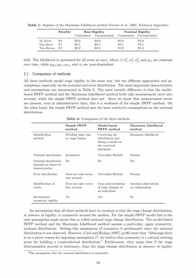
Table 1: Regimes of the Maximum Likelihood method (Goette et al., 2007, Technical Appendix)

Flexible Real Rigidity Nominal RigidityConstrained Unconstrained Constrained Unconstrained

No Error F0 RC0 RU0 NC0 NU0One Error F1 RC1 RU1 NC1 NU1Two Errors F2 RC2 RU2 NC2 NU2

0.05. The likelihood is optimized for all years at once, where β, σ2ω, σ

2π, σ

2m and pm are constant

over time, while pR,t, pF,t, pN,t and πt are year-dependent.

2.1 Comparison of methods

All three methods model wage rigidity in the same way, but use different approaches and as-sumptions, especially on the notional and error distribution. The most important characteristicsand assumptions are summarized in Table 2. The most notable difference is that the model-based IWFP method and the Maximum Likelihood method both take measurement error intoaccount, while the simple IWFP method does not. Since we know that measurement errorsare present, even in administrative data, this is a weakness of the simple IWFP method. Onthe other hand, the simple IWFP method uses the least restrictive assumptions on the notionaldistribution.

Table 2: Comparison of the three methods

Simple IWFPmethod

Model-basedIWFP method

Maximum Likelihoodmethod

Identificationmethod

Dividing wage cutsby wage freezes

Correcting thedistribution andfitting a model onthe correctedhistogram

Maximum Likelihood

Notional distribution Symmetric Two-sided Weibull Normal

Notional distributiondepends on observedcharacteristics

No No Yes

Error distribution Does not take errorsinto account

Two-sided Weibull Normal

Identification oferrors

Does not take errorsinto account

Uses autocorrelationof wage changes ofan individual

Assumes observationsare independent

Incorporatessymmetric rigidity

No Yes No

An assumption that all three methods have in common is that the wage change distribution,in absence of rigidity, is symmetric around the median. For the simple IWFP model this is theonly assumption made about this so called notional wage change distribution. The model-basedIWFP method and the Maximum Likelihood method assume a particular, again symmetric,notional distribution. Testing this assumption of symmetry is problematic since the notionaldistribution is not observed. However, Card and Hyslop (1997) (p.86) state that “Although thereis no a priori reason for imposing assumption 14, we believe that symmetry is a natural startingpoint for building a counterfactual distribution.” Furthermore, they argue that if the wagedetermination process is stationary, than the wage change distribution in absence of rigidity

4The assumption that the notional distribution is symmetric

10

is symmetric. Another argument for using the symmetry assumption is found in Dickens andGoette (2005) (p. 11), where the authors state that “The lower tail, in countries where realrigidity does not appear to be much of a problem, seems to be a mirror image of the uppertail for those parts that are above zero when the distribution is not affected by real rigidity.”If one does not want to use the symmetry assumption, one needs to assume that the shape ofthe wage change distribution is constant over time. This assumption is used in Kahn (1997).

The model-based based method and Maximum Likelihood method make additional assump-tions about the notional distribution of wage changes. The model-based IWFP method assumesthat notional wage changes are two-sided Weibull distributed, while the Maximum Likelihoodmethods assumes that wage changes come from a normal distribution. In Goette et al. (2007) anormal distribution is chosen. In Dickens and Goette (2005) (p. 11) the normality assumptionis criticized: “an analysis of Gottschalk’s estimates of true wages, suggests that wage changeshave a distribution that is both more peaked and has fatter tails than the normal”. Dickenset al. (2007a)(p. 204) give some arguments for assuming a two-sided Weibull: “A Weibull dis-tribution will provide a good approximation to the distribution if, instead, workers’ raises arebased on sequential standards, where only those who meet all prior standards are considered forthe next level, and at each level, rewards increase exponentially.” In addition Lunnemann andWintr (2010) (p. 25) state that “This choice is based on the observation that the distribution ofwage changes is typically more peaked and has fatter tails than the normal distribution.” Katay(2011) (p. 10) gives similar arguments “The motivation behind using a two-sided Weibull distri-bution is that a typical wage change distribution clearly diverges from the normal distributioneven at the right tail unaffected by rigidity: workers’ wage changes are tightly clustered aroundthe median change, which makes the distribution much more peaked with fatter tails comparedto the normal.” The Maximum Likelihood method is the only method which uses explanatoryvariables to construct the notional distribution. This has the advantage that heterogeneity is,partially, taken into account.

Also the assumptions on the error distribution differ. Where the simple IWFP method doesnot take errors into account at all, the ML method assumes that they are normally distributed.The model-based IWFP method assumes that errors are two-sided Weibull distributed. InDickens and Goette (2005) (p. 5) this assumption is substantiated as follows: “This structurefor the error – the two-sided Weibull with a fraction of people never making errors – was chosento match the distribution of eimated errors in Gottschalk’s data. His estimated errors had adistinctly peaked distribution and showed some auto-correlation in the probability of an errorthat was simply accounted for by having a group of people who didn’t make errors.” Furthermorethe model-based IWFP method uses the autocorrelation that is caused by measurement errorsto identify the extent of measurement error. The Maximum Likelihood method assumes thatall observations are independent and does not use this property.

All three methods have their own strengths and weaknesses. In an ideal situation we wouldpropose to combine the strengths of the various methods by identifying two-sided Weibull-distributed measurement error using the autocorrelation in the wage changes and let the two-sided Weibull distributed notional distribution depend on observed characteristics. As an at-tempt to integrate the strong points of the different methods we have tried to adapt the Max-imum Likelihood method to allow for a two-sided Weibull wage change and error distribution.However, it turned out that this is infeasible since analytical expressions for the required in-tegrals of two-sided Weibull distributions are not available. This would mean that for everyobservation and iteration the integrals should be approximated numerically. Given our largesample size (26,601,768 observations) this is not feasible, unfortunately. It would be an inter-esting topic for further research.

However, if we have to make a choice for a particular method, then we would choose themodel-based IWFP method. Although this method does not take heterogeneity in wage changesinto account, the notional distribution is flexible and more realistic than the normal distribution

11

of the Maximum Likelihood method. Furthermore this method takes measurement error intoaccount and uses additional information (autocorrelation) to identify it. A second-best wouldbe the Maximum Likelihood method which also accounts for measurement error.

The DNWR-estimates of the IWFP methods and the Maximum Likelihood method can notbe compared directly. Both IWFP methods estimate the probability of being covered by DNWRby inspecting the workers with nominal wage cuts and freezes. Therefore, these estimates ofDNWR only give information on those not covered by DRWR, since if they would have beencovered by DRWR they would not have had a wage cut or freeze. In fact, here DNWR can beinterpreted as the probability of being covered by DNWR, conditional on not being covered byDRWR. The Maximum Likelihood method however, assumes that observations can be in onlyone out of three regimes (the flexible regime, the nominal rigidity regime or the real rigidityregime). Here the regime probabilities add up to unity by construction. This clearly is nota conditional probability. To make our estimates comparable with each other, we will alsoreport DNWR estimates for the Maximum Likelihood method according to the definitions ofthe IWFP, since this definition is used most often in the literature. Hence, we calculate theprobability of being covered by nominal wage rigidity, conditional on not being covered by realwage rigidity as follows:

P cN,t =PN,t

PF,t + PN,t=

PN,t1 − PR,t

(9)

3 Data

Data from the Social Statistical files (SSB) for the Netherlands regarding the years 2006-2012is used. The wage data is based on the policy administration of the Employee InsurancesImplementing Agency (UWV). In this data set wage information is available per month (for mostof the observations). The data set does also contain information on salaried hours (‘verloondeuren’). Furthermore various characteristics of the employees and their jobs are available, rangingfrom the obtained level of education to contract type.

Regarding wage changes different measures could be used. The most common measuresfocus on hourly wages or annual earnings. Within the IWFP both are used (Dickens et al.,2007a). The procedure for correcting measurement errors and estimating rigidity is slightlydifferent for both measures. Often annual earnings are converted to hourly wages (Dickenset al., 2007a; Du Caju et al., 2007). However it is widely acknowledged (Dickens et al., 2007a;Lunnemann and Wintr, 2010; Gottschalk, 2005) that measures for hours worked are imprecise.

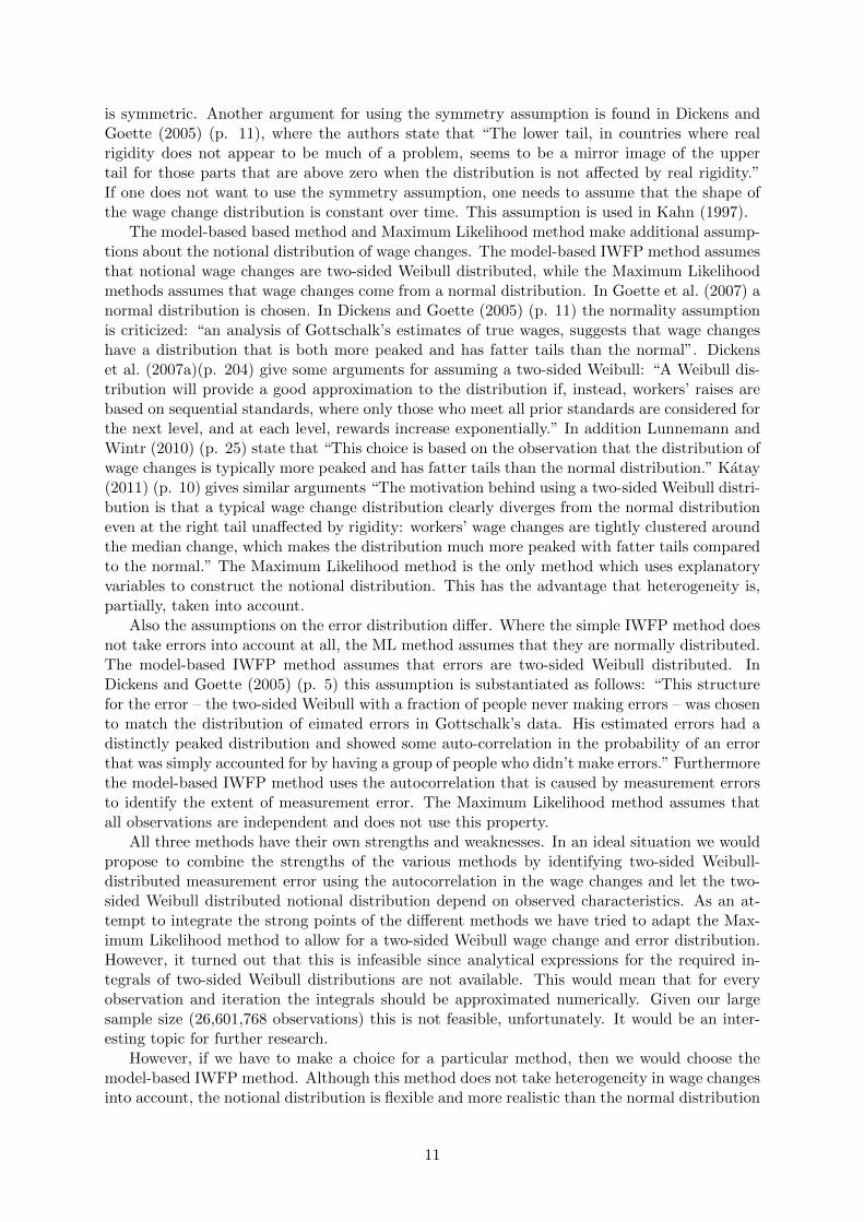
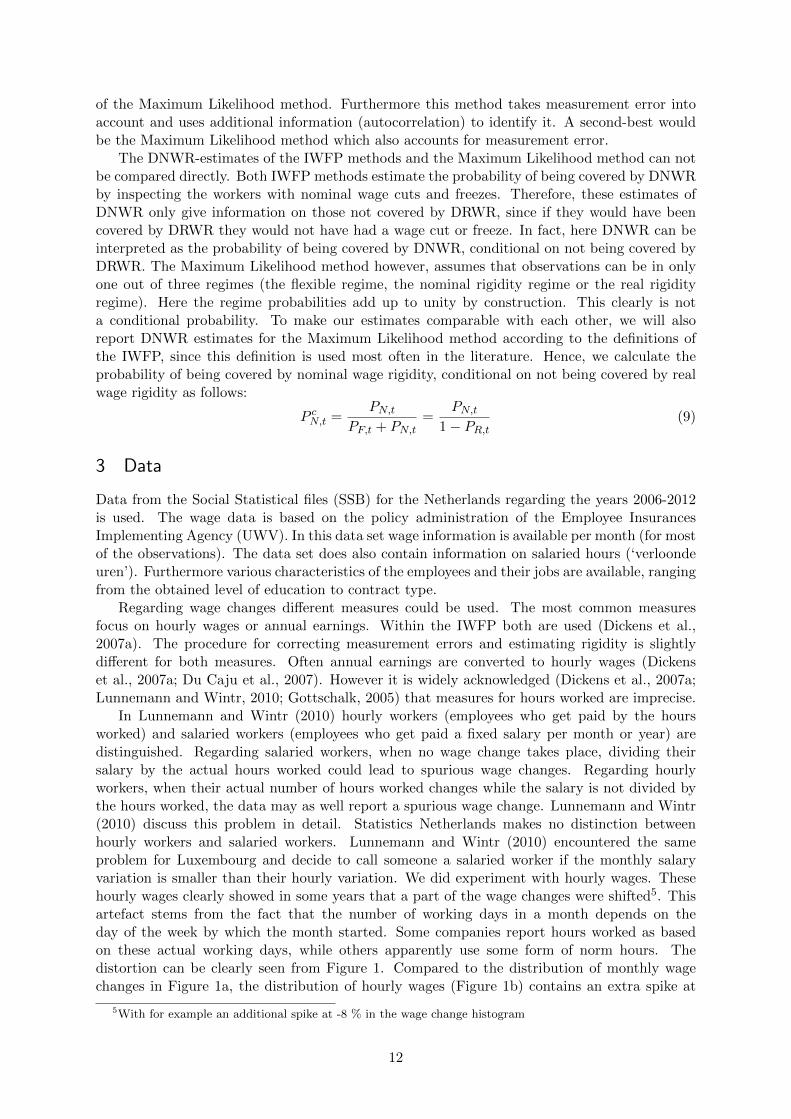
In Lunnemann and Wintr (2010) hourly workers (employees who get paid by the hoursworked) and salaried workers (employees who get paid a fixed salary per month or year) aredistinguished. Regarding salaried workers, when no wage change takes place, dividing theirsalary by the actual hours worked could lead to spurious wage changes. Regarding hourlyworkers, when their actual number of hours worked changes while the salary is not divided bythe hours worked, the data may as well report a spurious wage change. Lunnemann and Wintr(2010) discuss this problem in detail. Statistics Netherlands makes no distinction betweenhourly workers and salaried workers. Lunnemann and Wintr (2010) encountered the sameproblem for Luxembourg and decide to call someone a salaried worker if the monthly salaryvariation is smaller than their hourly variation. We did experiment with hourly wages. Thesehourly wages clearly showed in some years that a part of the wage changes were shifted5. Thisartefact stems from the fact that the number of working days in a month depends on theday of the week by which the month started. Some companies report hours worked as basedon these actual working days, while others apparently use some form of norm hours. Thedistortion can be clearly seen from Figure 1. Compared to the distribution of monthly wagechanges in Figure 1a, the distribution of hourly wages (Figure 1b) contains an extra spike at

5With for example an additional spike at -8 % in the wage change histogram

12

the left hand side due to firms that report an increase in actual working hours because October2012 contains more working days (opposed to weekend-days) than October 2011, while thesalary is not sensitive to this change in working days. Furthermore, hourly workers are veryuncommon in the Netherlands. For these reasons we do not divide wages by the number ofhours worked. In this study, we focus on the year to year changes in the monthly base wage forthe month of October. In October no specific incidental wage changes take place, which coulddistort our estimates. Using monthly in stead of hourly wages prevents us from introducingmeasurement errors. However, measurement error will to some extent still be present in ourdata, for example because firms may accidentily register bonuses and declarations as part ofthe base wage. According to the model-based IWFP method 83% of the jobs report the wagealways without measurement error, for the other 17% an error is introduced in 82% of the cases.

0

100,000

200,000

300,000

400,000

500,000

600,000

-35% -25% -15% -5% 5% 15% 25% 35% 45% 55%

Fre

qu

en

cy

(a) Observed hourly wage change distribution

0

100,000

200,000

300,000

400,000

500,000

600,000

-35% -25% -15% -5% 5% 15% 25% 35% 45% 55%

Fre

qu

en

cy

(b) Observed monthly wage change distribution

Source: own calculations based on Statistics Netherlands microdata

Figure 1: Histograms of the observed wage change distributions in 2012

Table 3: Descriptive statistics of the observed monthly wage change distributions

Year N Mean Median Skewness Kurtosis SD do < 0 do < πML do < πCEP

2007 4431928 0.054 0.034 2.149 108.955 0.224 16% 33% 25%2008 4489885 0.058 0.042 1.978 115.405 0.213 15% 34% 33%2009 4609207 0.038 0.029 1.498 139.087 0.206 20% 42% 31%2010 4652883 0.030 0.015 2.338 149.772 0.206 21% 45% 49%2011 4626283 0.032 0.021 1.143 136.259 0.187 20% 41% 49%2012 4388473 0.033 0.023 0.226 154.240 0.189 19% 42% 46%

Source: own calculations based on Statistics Netherlands microdataNote: The estimated inflation expectations of the ML-model (the inflation expectations published at that time)are for 2007: 2.032% (1.250%); 2008: 2.730% (2.625%); 2009: 2.182% (1.000%); 2010: 1.092% (1.375%); 2011:1.417% (2.000%); 2012: 1.818% (2.000%).

To make the estimates comparable with other studies we confine the analysis to job-stayers.In some previous studies part-timers are removed from the sample6, but since part-time workis very common in the Netherlands (more than half of all employees are part-time workers) weinclude those observations. Because job mobility remains the major channel to adjust workinghours (Fouarge and Baaijens (2004)), including part-time workers will not lead to biassed results.Furthermore we remove some implausible observations. Wage cuts of more than 35 % and wageincreases of more than 60 % in the simple IWFP and Maximum Likelihood method, since thoseobservations are unlikely to reflect valid wage changes. Furthermore Dickens et al. (2007a) usethe same bounds. This reduces our sample with 2 %. For the model-based IWFP we do not

6For example: Messina et al. (2010), Du Caju et al. (2007)

13

0

100,000

200,000

300,000

400,000

500,000

600,000

-35% -25% -15% -5% 5% 15% 25% 35% 45% 55%

Fre

qu

en

cy

(a) 2007

0

100,000

200,000

300,000

400,000

500,000

600,000

-35% -25% -15% -5% 5% 15% 25% 35% 45% 55%

Fre

qu

en

cy

(b) 2008

0

100,000

200,000

300,000

400,000

500,000

600,000

-35% -25% -15% -5% 5% 15% 25% 35% 45% 55%

Fre

qu

en

cy

(c) 2009

0

100,000

200,000

300,000

400,000

500,000

600,000

-35% -25% -15% -5% 5% 15% 25% 35% 45% 55%

Fre

qu

en

cy

(d) 2010

0

100,000

200,000

300,000

400,000

500,000

600,000

-35% -25% -15% -5% 5% 15% 25% 35% 45% 55%

Fre

qu

en

cy

(e) 2011

0

100,000

200,000

300,000

400,000

500,000

600,000

-35% -25% -15% -5% 5% 15% 25% 35% 45% 55%

Fre

qu

en

cy

(f) 2012

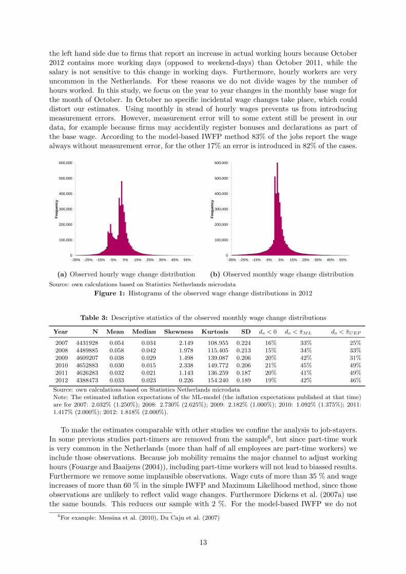
Source: own calculations based on Statistics Netherlands microdata

Figure 2: Histograms of the observed monthly wage change distributions

14

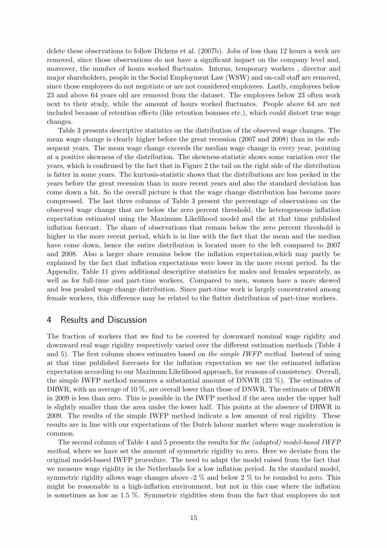
delete these observations to follow Dickens et al. (2007b). Jobs of less than 12 hours a week areremoved, since those observations do not have a significant impact on the company level and,moreover, the number of hours worked fluctuates. Interns, temporary workers , director andmajor shareholders, people in the Social Employment Law (WSW) and on-call staff are removed,since those employees do not negotiate or are not considered employees. Lastly, employees below23 and above 64 years old are removed from the dataset. The employees below 23 often worknext to their study, while the amount of hours worked fluctuates. People above 64 are notincluded because of retention effects (like retention bonuses etc.), which could distort true wagechanges.

Table 3 presents descriptive statistics on the distribution of the observed wage changes. Themean wage change is clearly higher before the great recession (2007 and 2008) than in the sub-sequent years. The mean wage change exceeds the median wage change in every year, pointingat a positive skewness of the distribution. The skewness-statistic shows some variation over theyears, which is confirmed by the fact that in Figure 2 the tail on the right side of the distributionis fatter in some years. The kurtosis-statistic shows that the distributions are less peeked in theyears before the great recession than in more recent years and also the standard deviation hascome down a bit. So the overall picture is that the wage change distribution has become morecompressed. The last three columns of Table 3 present the percentage of observations on theobserved wage change that are below the zero percent threshold, the heterogeneous inflationexpectation estimated using the Maximum Likelihood model and the at that time publishedinflation forecast. The share of observations that remain below the zero percent threshold ishigher in the more recent period, which is in line with the fact that the mean and the medianhave come down, hence the entire distribution is located more to the left compared to 2007and 2008. Also a larger share remains below the inflation expectation,which may partly beexplained by the fact that inflation expectations were lower in the more recent period. In theAppendix, Table 11 gives additional descriptive statistics for males and females separately, aswell as for full-time and part-time workers. Compared to men, women have a more skewedand less peaked wage change distribution. Since part-time work is largely concentrated amongfemale workers, this difference may be related to the flatter distribution of part-time workers.

4 Results and Discussion

The fraction of workers that we find to be covered by downward nominal wage rigidity anddownward real wage rigidity respectively varied over the different estimation methods (Table 4and 5). The first column shows estimates based on the simple IWFP method. Instead of usingat that time published forecasts for the inflation expectation we use the estimated inflationexpectation according to our Maximum Likelihood approach, for reasons of consistency. Overall,the simple IWFP method measures a substantial amount of DNWR (23 %). The estimates ofDRWR, with an average of 10 %, are overall lower than those of DNWR. The estimate of DRWRin 2009 is less than zero. This is possible in the IWFP method if the area under the upper halfis slightly smaller than the area under the lower half. This points at the absence of DRWR in2009. The results of the simple IWFP method indicate a low amount of real rigidity. Theseresults are in line with our expectations of the Dutch labour market where wage moderation iscommon.

The second column of Table 4 and 5 presents the results for the (adapted) model-based IWFPmethod, where we have set the amount of symmetric rigidity to zero. Here we deviate from theoriginal model-based IWFP procedure. The need to adapt the model raised from the fact thatwe measure wage rigidity in the Netherlands for a low inflation period. In the standard model,symmetric rigidity allows wage changes above -2 % and below 2 % to be rounded to zero. Thismight be reasonable in a high-inflation environment, but not in this case where the inflationis sometimes as low as 1.5 %. Symmetric rigidities stem from the fact that employers do not

15

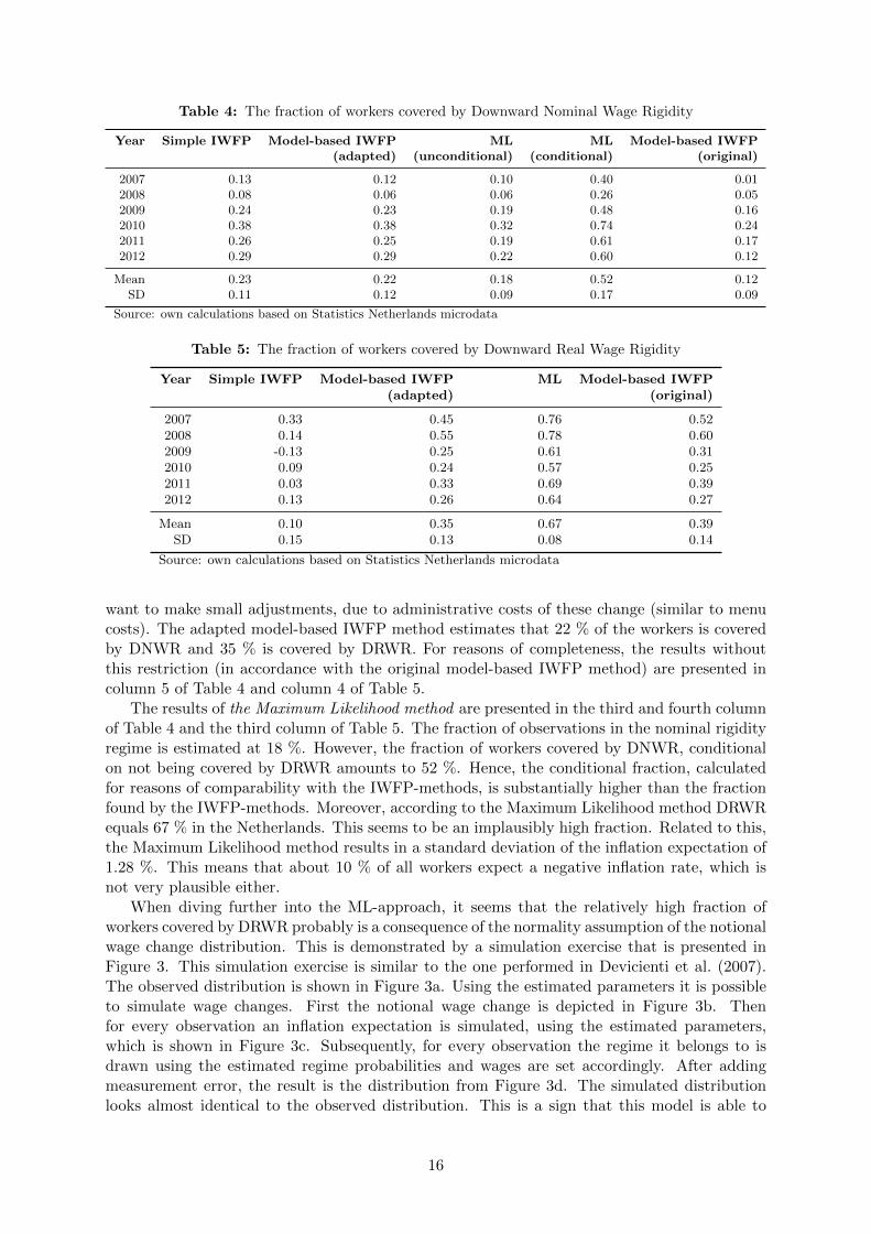
Table 4: The fraction of workers covered by Downward Nominal Wage Rigidity

Year Simple IWFP Model-based IWFP ML ML Model-based IWFP(adapted) (unconditional) (conditional) (original)

2007 0.13 0.12 0.10 0.40 0.012008 0.08 0.06 0.06 0.26 0.052009 0.24 0.23 0.19 0.48 0.162010 0.38 0.38 0.32 0.74 0.242011 0.26 0.25 0.19 0.61 0.172012 0.29 0.29 0.22 0.60 0.12

Mean 0.23 0.22 0.18 0.52 0.12SD 0.11 0.12 0.09 0.17 0.09

Source: own calculations based on Statistics Netherlands microdata

Table 5: The fraction of workers covered by Downward Real Wage Rigidity

Year Simple IWFP Model-based IWFP ML Model-based IWFP(adapted) (original)

2007 0.33 0.45 0.76 0.522008 0.14 0.55 0.78 0.602009 -0.13 0.25 0.61 0.312010 0.09 0.24 0.57 0.252011 0.03 0.33 0.69 0.392012 0.13 0.26 0.64 0.27

Mean 0.10 0.35 0.67 0.39SD 0.15 0.13 0.08 0.14

Source: own calculations based on Statistics Netherlands microdata

want to make small adjustments, due to administrative costs of these change (similar to menucosts). The adapted model-based IWFP method estimates that 22 % of the workers is coveredby DNWR and 35 % is covered by DRWR. For reasons of completeness, the results withoutthis restriction (in accordance with the original model-based IWFP method) are presented incolumn 5 of Table 4 and column 4 of Table 5.

The results of the Maximum Likelihood method are presented in the third and fourth columnof Table 4 and the third column of Table 5. The fraction of observations in the nominal rigidityregime is estimated at 18 %. However, the fraction of workers covered by DNWR, conditionalon not being covered by DRWR amounts to 52 %. Hence, the conditional fraction, calculatedfor reasons of comparability with the IWFP-methods, is substantially higher than the fractionfound by the IWFP-methods. Moreover, according to the Maximum Likelihood method DRWRequals 67 % in the Netherlands. This seems to be an implausibly high fraction. Related to this,the Maximum Likelihood method results in a standard deviation of the inflation expectation of1.28 %. This means that about 10 % of all workers expect a negative inflation rate, which isnot very plausible either.

When diving further into the ML-approach, it seems that the relatively high fraction ofworkers covered by DRWR probably is a consequence of the normality assumption of the notionalwage change distribution. This is demonstrated by a simulation exercise that is presented inFigure 3. This simulation exercise is similar to the one performed in Devicienti et al. (2007).The observed distribution is shown in Figure 3a. Using the estimated parameters it is possibleto simulate wage changes. First the notional wage change is depicted in Figure 3b. Thenfor every observation an inflation expectation is simulated, using the estimated parameters,which is shown in Figure 3c. Subsequently, for every observation the regime it belongs to isdrawn using the estimated regime probabilities and wages are set accordingly. After addingmeasurement error, the result is the distribution from Figure 3d. The simulated distributionlooks almost identical to the observed distribution. This is a sign that this model is able to

16

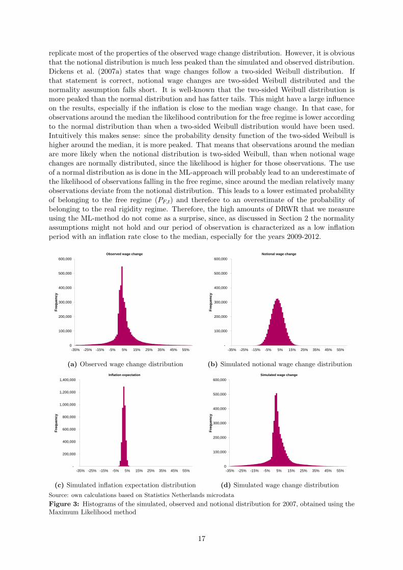
replicate most of the properties of the observed wage change distribution. However, it is obviousthat the notional distribution is much less peaked than the simulated and observed distribution.Dickens et al. (2007a) states that wage changes follow a two-sided Weibull distribution. Ifthat statement is correct, notional wage changes are two-sided Weibull distributed and thenormality assumption falls short. It is well-known that the two-sided Weibull distribution ismore peaked than the normal distribution and has fatter tails. This might have a large influenceon the results, especially if the inflation is close to the median wage change. In that case, forobservations around the median the likelihood contribution for the free regime is lower accordingto the normal distribution than when a two-sided Weibull distribution would have been used.Intuitively this makes sense: since the probability density function of the two-sided Weibull ishigher around the median, it is more peaked. That means that observations around the medianare more likely when the notional distribution is two-sided Weibull, than when notional wagechanges are normally distributed, since the likelihood is higher for those observations. The useof a normal distribution as is done in the ML-approach will probably lead to an underestimate ofthe likelihood of observations falling in the free regime, since around the median relatively manyobservations deviate from the notional distribution. This leads to a lower estimated probabilityof belonging to the free regime (PF,t) and therefore to an overestimate of the probability ofbelonging to the real rigidity regime. Therefore, the high amounts of DRWR that we measureusing the ML-method do not come as a surprise, since, as discussed in Section 2 the normalityassumptions might not hold and our period of observation is characterized as a low inflationperiod with an inflation rate close to the median, especially for the years 2009-2012.

0

100,000

200,000

300,000

400,000

500,000

600,000

-35% -25% -15% -5% 5% 15% 25% 35% 45% 55%

Fre

qu

en

cy

Observed wage change

(a) Observed wage change distribution

-

100,000

200,000

300,000

400,000

500,000

600,000

-35% -25% -15% -5% 5% 15% 25% 35% 45% 55%

Fre

qu

en

cy

Notional wage change

(b) Simulated notional wage change distribution

-

200,000

400,000

600,000

800,000

1,000,000

1,200,000

1,400,000

-35% -25% -15% -5% 5% 15% 25% 35% 45% 55%

Fre

qu

en

cy

Inflation expectation

(c) Simulated inflation expectation distribution

0

100,000

200,000

300,000

400,000

500,000

600,000

-35% -25% -15% -5% 5% 15% 25% 35% 45% 55%

Fre

qu

en

cy

Simulated wage change

(d) Simulated wage change distribution

Source: own calculations based on Statistics Netherlands microdata

Figure 3: Histograms of the simulated, observed and notional distribution for 2007, obtained using theMaximum Likelihood method

17

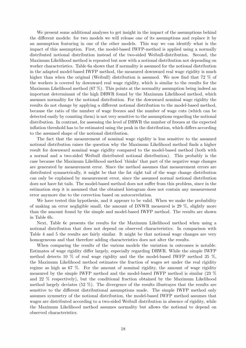
We present some additional analyses to get insight in the impact of the assumptions behindthe different models: for two models we will release one of its assumptions and replace it byan assumption featuring in one of the other models. This way we can identify what is theimpact of this assumption. First, the model-based IWFP-method is applied using a normallydistributed notional distribution instead of the two-sided Weibull-distribution. Second, theMaximum Likelihood method is repeated but now with a notional distribution not depending onworker characteristics. Table 6a shows that if normality is assumed for the notional distributionin the adapted model-based IWFP method, the measured downward real wage rigidity is muchhigher than when the original (Weibull) distribution is assumed. We now find that 72 % ofthe workers is covered by downward real wage rigidity, which is similar to the results for theMaximum Likelihood method (67 %). This points at the normality assumption being indeed animportant determinant of the high DRWR found by the Maximum Likelihood method, whichassumes normality for the notional distribution. For the downward nominal wage rigidity theresults do not change by applying a different notional distribution to the model-based method,because the ratio of the number of wage freezes and the number of wage cuts (which can bedetected easily by counting them) is not very sensitive to the assumptions regarding the notionaldistribution. In contrast, for assessing the level of DRWR the number of freezes at the expectedinflation threshold has to be estimated using the peak in the distribution, which differs accordingto the assumed shape of the notional distribution.

The fact that the measurement of nominal wage rigidity is less sensitive to the assumednotional distribution raises the question why the Maximum Likelihood method finds a higherresult for downward nominal wage rigidity compared to the model-based method (both witha normal and a two-sided Weibull distributed notional distribution). This probably is thecase because the Maximum Likelihood method ’thinks’ that part of the negative wage changesare generated by measurement error. Since the method assumes that measurement errors aredistributed symmetrically, it might be that the fat right tail of the wage change distributioncan only be explained by measurement error, since the assumed normal notional distributiondoes not have fat tails. The model-based method does not suffer from this problem, since in theestimation step it is assumed that the obtained histogram does not contain any measurementerror anymore due to the correction based on autocorrelation.

We have tested this hypothesis, and it appears to be valid. When we make the probabilityof making an error negligible small, the amount of DNWR measured is 29 %, slightly morethan the amount found by the simple and model-based IWFP method. The results are shownin Table 6b.

Next, Table 6c presents the results for the Maximum Likelihood method when using anotional distribution that does not depend on observed characteristics. In comparison withTable 4 and 5 the results are fairly similar. It might be that notional wage changes are veryhomogeneous and that therefore adding characteristics does not alter the results.

When comparing the results of the various models the variation in outcomes is notable.Estimates of wage rigidity differ largely, especially regarding DRWR. While the simple IWFPmethod detects 10 % of real wage rigidity and the the model-based IWFP method 35 %,the Maximum Likelihood method estimates the fraction of wages set under the real rigidityregime as high as 67 %. For the amount of nominal rigidity, the amount of wage rigiditymeasured by the simple IWFP method and the model-based IWFP method is similar (23 %and 22 % respectively), but the conditional fraction obtained by the Maximum Likelihoodmethod largely deviates (52 %). The divergence of the results illustrayes that the results aresensitive to the different distributional assumptions made. The simple IWFP method onlyassumes symmetry of the notional distribution, the model-based IWFP method assumes thatwages are distributed according to a two-sided Weibull distribution in absence of rigidity, whilethe Maximum Likelihood method assumes normality but allows the notional to depend onobserved characteristics.

18

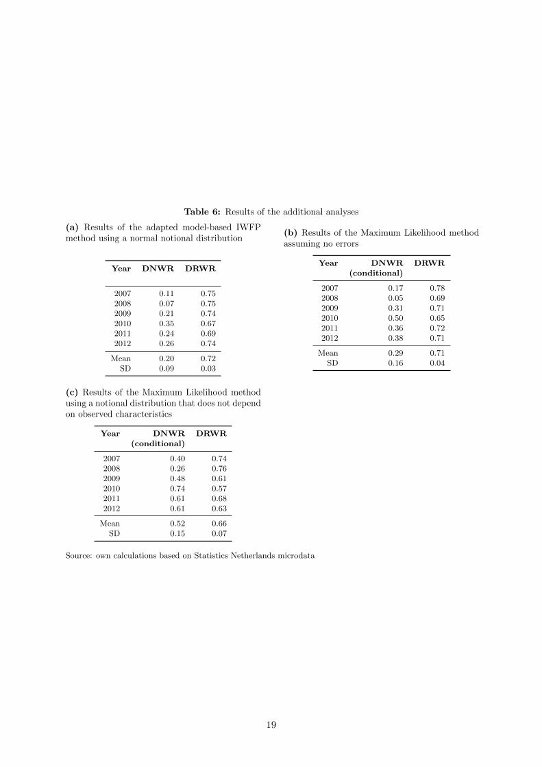
Table 6: Results of the additional analyses

(a) Results of the adapted model-based IWFPmethod using a normal notional distribution

Year DNWR DRWR

2007 0.11 0.752008 0.07 0.752009 0.21 0.742010 0.35 0.672011 0.24 0.692012 0.26 0.74

Mean 0.20 0.72SD 0.09 0.03

(b) Results of the Maximum Likelihood methodassuming no errors

Year DNWR DRWR(conditional)

2007 0.17 0.782008 0.05 0.692009 0.31 0.712010 0.50 0.652011 0.36 0.722012 0.38 0.71

Mean 0.29 0.71SD 0.16 0.04

(c) Results of the Maximum Likelihood methodusing a notional distribution that does not dependon observed characteristics

Year DNWR DRWR(conditional)

2007 0.40 0.742008 0.26 0.762009 0.48 0.612010 0.74 0.572011 0.61 0.682012 0.61 0.63

Mean 0.52 0.66SD 0.15 0.07

Source: own calculations based on Statistics Netherlands microdata

19

As discussed in the second section, the literature emphasizes that the normality assumptionis not very realistic, since the disribution of wage changes is supposed to be more peaked andhas fatter tales than the normal distribution. Our empirical analysis convincingly shows thatthe results are sensitive to the distributional assumptions regarding the notional wage changedistribution. The Maximum Likelihood method measures a much higher level than the modelbased IWFP method. Applying the normality assumption to the adapted model-based IWFPmethod, the measured downward real wage rigidity is much higher than when the original(Weibull) distribution is assumed. We therefore argue that the normality assumption in theMaximum Likelihood approach most probably leads to an overestimation of DRWR. A drawbackof the simple IWFP approach is that the measurement of wage rigidity is very sensitive to thespecified rate of inflation, since the estimation of the inflation expectation is not incorperatedin the model. Also, the simple model does not take into account measurement errors. Themodel-based approach has the most sophisticated method to take into account measurementerror. Given these empirical results we conclude that the model-based IWFP approach is thepreferred model of the three.

We find that, irregardless of the method used, the estimates of DNWR and DRWR differover the years. The simple IWFP model even presents negative estimates of the fraction of wagesset under the real rigidity regime, pointing at the absence of DRWR. Another interesting ob-servation is the fact that, according to all methods, DNWR is lower in 2007 and 2008 comparedto 2009-2012, while DRWR -according to the model-based and ML estimates- is substantiallyhigher in 2007 and 2008 than in subsequent years. In 2007 and 2008 the estimated inflationexpectation of both the model-based and Maximum Likelihood method was considerably higherthan the years thereafter. In theory the estimates of wage rigidity should not depend on theinflation expectation, which would imply that the amount of DNWR has increased after 2008.However, Bauer et al. (2007) also find this pattern and attribute this finding to the theory ofAkerlof et al. (2000) that “when inflation is low, a significant number of people may ignoreinflation when setting wages and prices.” This might be the case for the Netherlands as well.

In order to compare our estimates internationally, Figure 4 and Figure 5 present estimatesfor several countries based on various recent papers. It is important to note that the timeperiod of different estimates is not (always) equal. The adapted model-based method for TheNetherlands can be compared to the model-based estimates for other countries. The need toadapt the model raised from the fact that we measure wage rigidity in the Netherlands for alow inflation period. The results for the other countries were measured in periods less recentperiod, with higher inflation.

The first thing to notice is that within countries estimates according to the three discussedmethods vary substantially. This is in line with our findings for the Netherlands. A partof the variability might be explained by the fact that the time periods and data sets of thevarious method differ. However, the differences between the IWFP methods and the MaximumLikelihood method appear to be smaller for other countries than for our data, especially withrespect to DNWR: the Maximum Likelihood estimate of DNWR lies in between those of themodel-based en simple IWFP method for the UK and Italy. This might be partially explainedby the fact that in our period of observation the inflation was relatively low, which might leadto a situation where the inflation is close to the median; as discussed before this might lead toan overestimate of DRWR by the Maximum Likelihood method.

In Table 7 we have ranked the estimates. From this figure we can see that although theestimates might differ, both IWFP methods produce a quite similar ranking. The Pearsonrank correlation coefficient is 0.46 and 0.72 for DNWR and DRWR, respectively for the IWFPmethods. The Pearson rank correlation for the ML estimates and the model-based IWFPmethod is 0.72 for real wage rigidity. For nominal rigidity the Pearson rank correlation isnegative. However, note that these two correlation coefficients are based on a small number ofobservations.

20

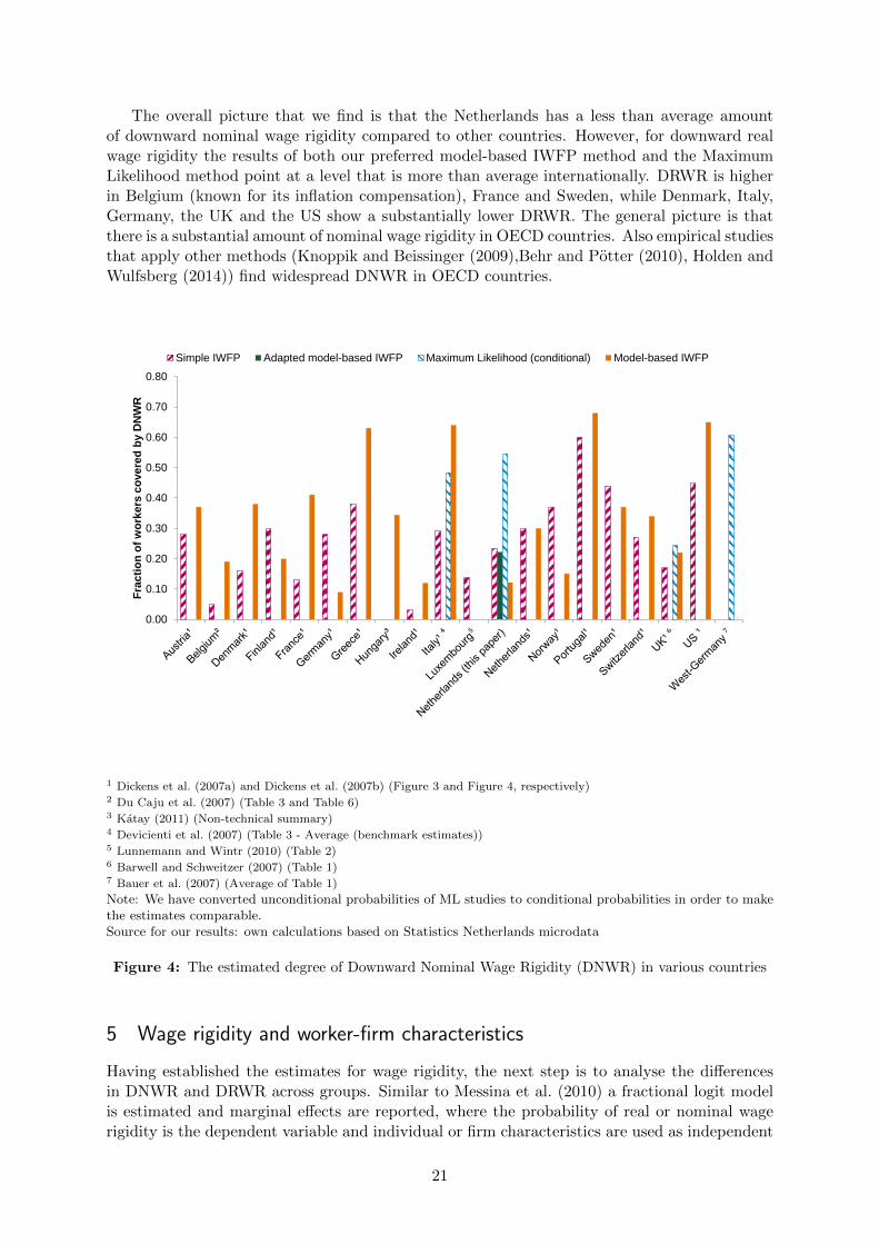
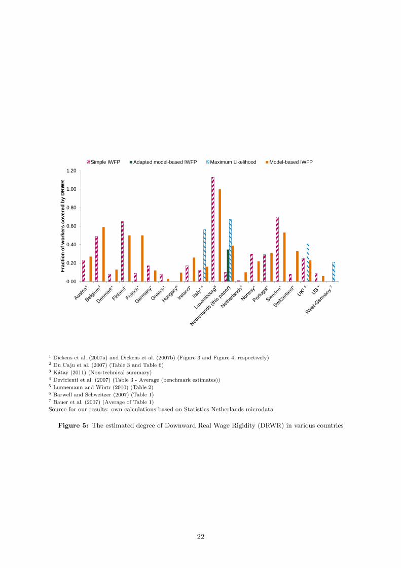
The overall picture that we find is that the Netherlands has a less than average amountof downward nominal wage rigidity compared to other countries. However, for downward realwage rigidity the results of both our preferred model-based IWFP method and the MaximumLikelihood method point at a level that is more than average internationally. DRWR is higherin Belgium (known for its inflation compensation), France and Sweden, while Denmark, Italy,Germany, the UK and the US show a substantially lower DRWR. The general picture is thatthere is a substantial amount of nominal wage rigidity in OECD countries. Also empirical studiesthat apply other methods (Knoppik and Beissinger (2009),Behr and Potter (2010), Holden andWulfsberg (2014)) find widespread DNWR in OECD countries.

0.00

0.10

0.20

0.30

0.40

0.50

0.60

0.70

0.80

Fra

cti

on

of

wo

rke

rs c

ove

red

by D

NW

R

Simple IWFP Adapted model-based IWFP Maximum Likelihood (conditional) Model-based IWFP

1 Dickens et al. (2007a) and Dickens et al. (2007b) (Figure 3 and Figure 4, respectively)2 Du Caju et al. (2007) (Table 3 and Table 6)3 Katay (2011) (Non-technical summary)4 Devicienti et al. (2007) (Table 3 - Average (benchmark estimates))5 Lunnemann and Wintr (2010) (Table 2)6 Barwell and Schweitzer (2007) (Table 1)7 Bauer et al. (2007) (Average of Table 1)

Note: We have converted unconditional probabilities of ML studies to conditional probabilities in order to makethe estimates comparable.Source for our results: own calculations based on Statistics Netherlands microdata

Figure 4: The estimated degree of Downward Nominal Wage Rigidity (DNWR) in various countries

5 Wage rigidity and worker-firm characteristics

Having established the estimates for wage rigidity, the next step is to analyse the differencesin DNWR and DRWR across groups. Similar to Messina et al. (2010) a fractional logit modelis estimated and marginal effects are reported, where the probability of real or nominal wagerigidity is the dependent variable and individual or firm characteristics are used as independent

21

0.00

0.20

0.40

0.60

0.80

1.00

1.20

Fra

cti

on

of

wo

rke

rs c

ove

red

by D

RW

R

Simple IWFP Adapted model-based IWFP Maximum Likelihood Model-based IWFP

1 Dickens et al. (2007a) and Dickens et al. (2007b) (Figure 3 and Figure 4, respectively)2 Du Caju et al. (2007) (Table 3 and Table 6)3 Katay (2011) (Non-technical summary)4 Devicienti et al. (2007) (Table 3 - Average (benchmark estimates))5 Lunnemann and Wintr (2010) (Table 2)6 Barwell and Schweitzer (2007) (Table 1)7 Bauer et al. (2007) (Average of Table 1)

Source for our results: own calculations based on Statistics Netherlands microdata

Figure 5: The estimated degree of Downward Real Wage Rigidity (DRWR) in various countries

22

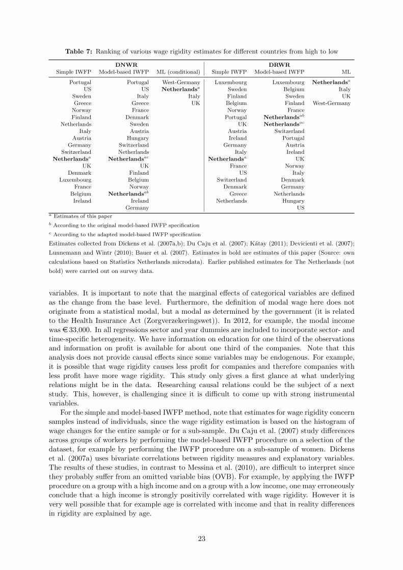
Table 7: Ranking of various wage rigidity estimates for different countries from high to low

DNWR DRWRSimple IWFP Model-based IWFP ML (conditional) Simple IWFP Model-based IWFP ML

Portugal Portugal West-Germany Luxembourg Luxembourg Netherlandsa

US US Netherlandsa Sweden Belgium ItalySweden Italy Italy Finland Sweden UKGreece Greece UK Belgium Finland West-Germany

Norway France Norway France

Finland Denmark Portugal Netherlandsab

Netherlands Sweden UK Netherlandsac

Italy Austria Austria SwitzerlandAustria Hungary Ireland Portugal

Germany Switzerland Germany AustriaSwitzerland Netherlands Italy Ireland

Netherlandsa Netherlandsac Netherlandsa UKUK UK France Norway

Denmark Finland US ItalyLuxembourg Belgium Switzerland Denmark

France Norway Denmark Germany

Belgium Netherlandsab Greece NetherlandsIreland Ireland Netherlands Hungary

Germany USa Estimates of this paper

b According to the original model-based IWFP specification

c According to the adapted model-based IWFP specification

Estimates collected from Dickens et al. (2007a,b); Du Caju et al. (2007); Katay (2011); Devicienti et al. (2007);

Lunnemann and Wintr (2010); Bauer et al. (2007). Estimates in bold are estimates of this paper (Source: own

calculations based on Statistics Netherlands microdata). Earlier published estimates for The Netherlands (not

bold) were carried out on survey data.

variables. It is important to note that the marginal effects of categorical variables are definedas the change from the base level. Furthermore, the definition of modal wage here does notoriginate from a statistical modal, but a modal as determined by the government (it is relatedto the Health Insurance Act (Zorgverzekeringswet)). In 2012, for example, the modal incomewas e 33,000. In all regressions sector and year dummies are included to incorporate sector- andtime-specific heterogeneity. We have information on education for one third of the observationsand information on profit is available for about one third of the companies. Note that thisanalysis does not provide causal effects since some variables may be endogenous. For example,it is possible that wage rigidity causes less profit for companies and therefore companies withless profit have more wage rigidity. This study only gives a first glance at what underlyingrelations might be in the data. Researching causal relations could be the subject of a nextstudy. This, however, is challenging since it is difficult to come up with strong instrumentalvariables.

For the simple and model-based IWFP method, note that estimates for wage rigidity concernsamples instead of individuals, since the wage rigidity estimation is based on the histogram ofwage changes for the entire sample or for a sub-sample. Du Caju et al. (2007) study differencesacross groups of workers by performing the model-based IWFP procedure on a selection of thedataset, for example by performing the IWFP procedure on a sub-sample of women. Dickenset al. (2007a) uses bivariate correlations between rigidity measures and explanatory variables.The results of these studies, in contrast to Messina et al. (2010), are difficult to interpret sincethey probably suffer from an omitted variable bias (OVB). For example, by applying the IWFPprocedure on a group with a high income and on a group with a low income, one may erroneouslyconclude that a high income is strongly positivily correlated with wage rigidity. However it isvery well possible that for example age is correlated with income and that in reality differencesin rigidity are explained by age.

23

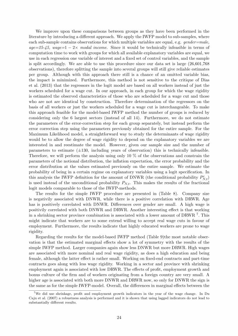
We improve upon these comparisons between groups as they have been performed in theliterature by introducing a different approach. We apply the IWFP model to sub-samples, whereeach sub-sample contains observations for which multiple variables are equal, e.g. gender=male,age=25-45, wage=1 − 2× modal income. Since it would be technically infeasible in terms ofcomputation time to work with groups for which all available explanatory variables are equal, weuse in each regression one variable of interest and a fixed set of control variables, and the sampleis split accordingly. We are able to use this procedure since our data set is large (26,601,768observations), therefore splitting the sample into several groups will still give reliable estimatesper group. Although with this approach there still is a chance of an omitted variable bias,the impact is minimized. Furthermore, this method is not sensitive to the critique of Diaset al. (2013) that the regressors in the logit model are based on all workers instead of just theworkers scheduled for a wage cut. In our approach, in each group for which the wage rigidityis estimated the observed characteristics of those who are scheduled for a wage cut and thosewho are not are identical by construction. Therefore determination of the regressors on thebasis of all workers or just the workers scheduled for a wage cut is interchangeable. To makethis approach feasible for the model-based IWFP method the number of groups is reduced byconsidering only the 6 largest sectors (instead of all 14). Furthermore, we do not estimatethe parameters of the error-correction step for each group separately, but instead perform theerror correction step using the parameters previously obtained for the entire sample. For theMaximum Likelihood model, a straightforward way to study the determinants of wage rigiditywould be to allow the degree of wage rigidity to depend on the explanatory variables we areinterested in and reestimate the model. However, given our sample size and the number ofparameters to estimate (±130, including years of observation) this is technically infeasible.Therefore, we will perform the analysis using only 10 % of the observations and constrain theparameters of the notional distribution, the inflation expectation, the error probability and theerror distribution at the values estimated previously on the entire sample. We estimate theprobability of being in a certain regime on explanatory variables using a logit specification. Inthis analysis the IWFP definition for the amount of DNWR (the conditional probability P cN,t)is used instead of the unconditional probability PN,t. This makes the results of the fractionallogit models comparable to those of the IWFP-methods.

The results for the simple IWFP procedure are presented in (Table 8). Company sizeis negativily associated with DNWR, while there is a positive correlation with DRWR. Agehas is positively correlated with DNWR. Differences over gender are small. A high wage ispositivily correlated with both DNWR and DRWR. Another interesting effect is that workingin a shrinking sector province combination is associated with a lower amount of DRWR 7. Thismight indicate that workers are to some extend willing to accept real wage cuts in favour ofemployment. Furthermore, the results indicate that highly educated workers are prone to wagerigidity.

Regarding the results for the model-based IWFP method (Table 9)the most notable obser-vation is that the estimated marginal effects show a lot of symmetry with the results of thesimple IWFP method. Larger companies again show less DNWR but more DRWR. High wagesare associated with more nominal and real wage rigidity, as does a high education and beingfemale, although the latter effect is rather small. Working on fixed-end contracts and part-timecontracts goes along with less wage rigidity. Working in a sector and province with shrinkingemployment again is associated with low DRWR. The effects of profit, employment growth andbonus culture of the firm and of workers originating from a foreign country are very small. Ahigher age is associated with both more DNWR and DRWR now, so only for DNWR the sign isthe same as for the simple IWFP-model. Overall, the differences in marginal effects between the

7We did use shrinkage, profit and employment growth indicators in the year of the wage change. In DuCaju et al. (2007) a robustness analysis is performed and it is shown that using lagged indicators do not lead tosubstantially different results.

24

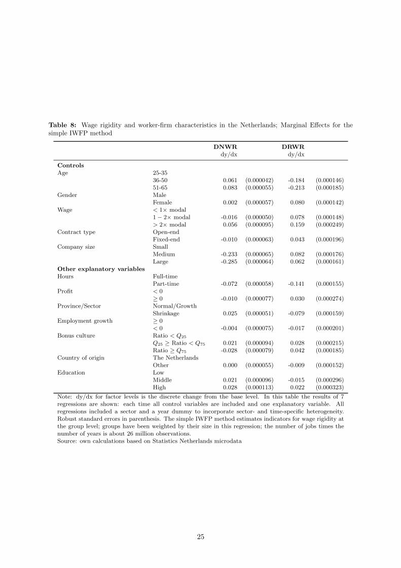
Table 8: Wage rigidity and worker-firm characteristics in the Netherlands; Marginal Effects for thesimple IWFP method

DNWR DRWRdy/dx dy/dx

ControlsAge 25-35

36-50 0.061 (0.000042) -0.184 (0.000146)51-65 0.083 (0.000055) -0.213 (0.000185)

Gender MaleFemale 0.002 (0.000057) 0.080 (0.000142)

Wage < 1× modal1 − 2× modal -0.016 (0.000050) 0.078 (0.000148)> 2× modal 0.056 (0.000095) 0.159 (0.000249)

Contract type Open-endFixed-end -0.010 (0.000063) 0.043 (0.000196)

Company size SmallMedium -0.233 (0.000065) 0.082 (0.000176)Large -0.285 (0.000064) 0.062 (0.000161)

Other explanatory variablesHours Full-time

Part-time -0.072 (0.000058) -0.141 (0.000155)Profit < 0

≥ 0 -0.010 (0.000077) 0.030 (0.000274)Province/Sector Normal/Growth

Shrinkage 0.025 (0.000051) -0.079 (0.000159)Employment growth ≥ 0

< 0 -0.004 (0.000075) -0.017 (0.000201)Bonus culture Ratio < Q25

Q25 ≥ Ratio < Q75 0.021 (0.000094) 0.028 (0.000215)Ratio ≥ Q75 -0.028 (0.000079) 0.042 (0.000185)

Country of origin The NetherlandsOther 0.000 (0.000055) -0.009 (0.000152)

Education LowMiddle 0.021 (0.000096) -0.015 (0.000296)High 0.028 (0.000113) 0.022 (0.000323)

Note: dy/dx for factor levels is the discrete change from the base level. In this table the results of 7regressions are shown: each time all control variables are included and one explanatory variable. Allregressions included a sector and a year dummy to incorporate sector- and time-specific heterogeneity.Robust standard errors in parenthesis. The simple IWFP method estimates indicators for wage rigidity atthe group level; groups have been weighted by their size in this regression; the number of jobs times thenumber of years is about 26 million observations.Source: own calculations based on Statistics Netherlands microdata

25

Table 9: Wage rigidity and worker-firm characteristics in the Netherlands; Marginal Effects for themodel-based IWFP method

DNWR DRWRdy/dx dy/dx

ControlsAge 25-35

36-50 0.061 (0.000046) 0.022 (0.000122)51-65 0.076 (0.000061) 0.058 (0.000150)

Gender MaleFemale 0.017 (0.000061) 0.038 (0.000134)

Wage < 1× modal1 − 2× modal -0.028 (0.000051) 0.016 (0.000130)> 2× modal 0.046 (0.000095) 0.117 (0.000205)

Contract type Open-endFixed-end -0.011 (0.000065) -0.011 (0.000166)

Company size SmallMedium -0.203 (0.000052) 0.045 (0.000128)Large -0.275 (0.000049) 0.018 (0.000118)

Other explanatory variablesHours Full-time

Part-time -0.095 (0.000058) -0.007 (0.000135)Profit < 0

≥ 0 -0.011 (0.000070) 0.023 (0.000175)Province/Sector Normal/Growth

Shrinkage 0.010 (0.000063) -0.065 (0.000140)Employment growth ≥ 0

< 0 0.007 (0.000082) 0.008 (0.000075)Bonus culture Ratio < Q25

Q25 ≥ Ratio < Q75 -0.013 (0.000173) 0.046 (0.000237)Ratio ≥ Q75 -0.009 (0.000128) 0.018 (0.000191)

Country of origin The NetherlandsOther -0.014 (0.000056) -0.004 (0.000121)

Education LowMiddle 0.021 (0.000103) 0.020 (0.000223)High 0.037 (0.000125) 0.057 (0.000263)

Note: dy/dx for factor levels is the discrete change from the base level. In this table the results of 7regressions are shown: each time all control variables are included and one explanatory variable. Allregressions included a sector and a year dummy to incorporate sector- and time-specific heterogeneity.Robust standard errors in parenthesis. The model based IWFP method estimates indicators for wagerigidity at the group level; groups have been weighted by their size in this regression; the number of jobstimes the number of years is about 26 million observations.Source: own calculations based on Statistics Netherlands microdata

26

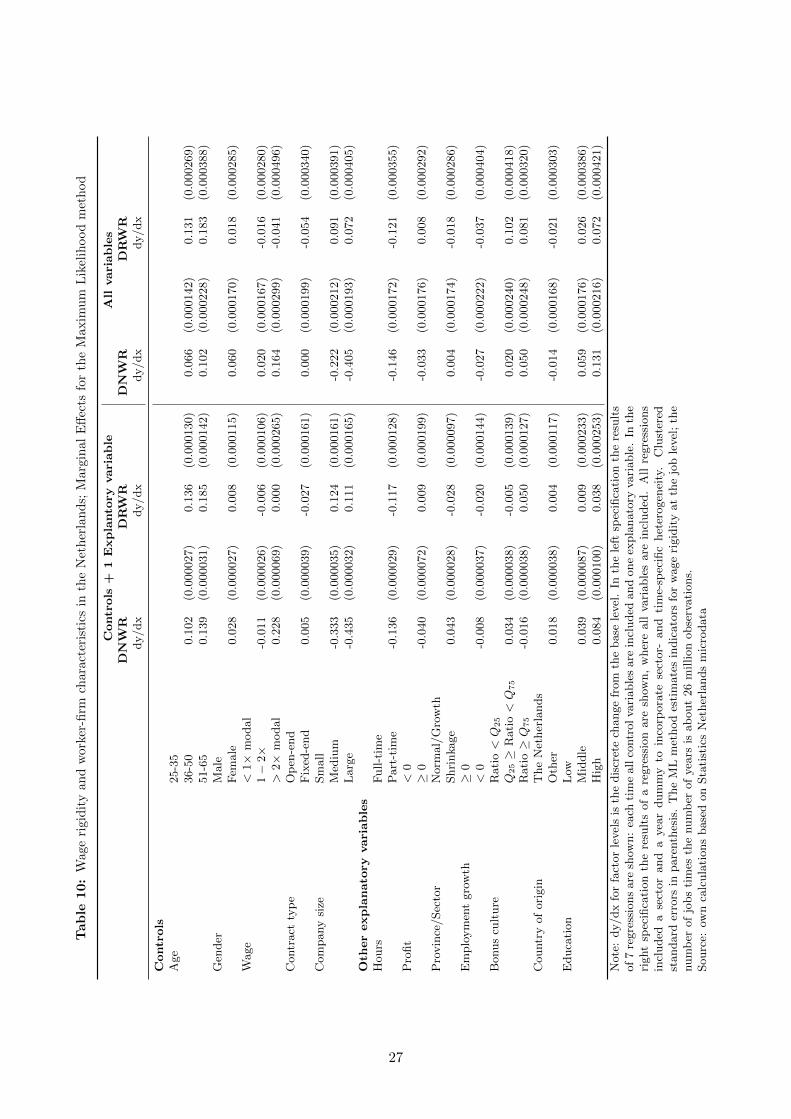
Tab

le10:

Wag

eri

gid

ity

and

wor

ker-

firm

chara

cter

isti

csin

the

Net

her

lan

ds;

Marg

inal

Eff

ects

for

the

Maxim

um

Lik

elih

ood

met

hod

Controls

+1Explanto

ryvariable

All

variables

DNW

RDRW

RDNW

RDRW

Rdy/dx

dy/dx

dy/dx

dy/dx

Controls

Age

25-3

536-5

00.1

02

(0.0

00027)

0.1

36

(0.0

00130)

0.0

66

(0.0

00142)

0.1

31

(0.0

00269)

51-6

50.1

39

(0.0

00031)

0.1

85

(0.0

00142)

0.1

02

(0.0

00228)

0.1

83

(0.0

00388)

Gen

der

Male

Fem

ale

0.0

28

(0.0

00027)

0.0

08

(0.0

00115)

0.0

60

(0.0

00170)

0.0

18

(0.0

00285)

Wage

<1×

modal

1−

2×

-0.0

11

(0.0

00026)

-0.0

06

(0.0

00106)

0.0

20

(0.0

00167)

-0.0

16

(0.0

00280)

>2×

modal

0.2

28

(0.0

00069)

0.0

00

(0.0

00265)

0.1

64

(0.0

00299)

-0.0

41

(0.0

00496)

Contr

act

typ

eO

pen

-end

Fix

ed-e

nd

0.0

05

(0.0

00039)

-0.0

27

(0.0

00161)

0.0

00

(0.0

00199)

-0.0

54

(0.0

00340)

Com

pany

size

Sm

all

Med

ium

-0.3

33

(0.0

00035)

0.1

24

(0.0

00161)

-0.2

22

(0.0

00212)

0.0

91

(0.0

00391)

Larg

e-0

.435

(0.0

00032)

0.1

11

(0.0

00165)

-0.4

05

(0.0

00193)

0.0

72

(0.0

00405)

Oth

erexplanato

ryvariables

Hours

Full-t

ime

Part

-tim

e-0

.136

(0.0

00029)

-0.1

17

(0.0

00128)

-0.1

46

(0.0

00172)

-0.1

21

(0.0

00355)

Pro

fit

<0

≥0

-0.0

40

(0.0

00072)

0.0

09

(0.0

00199)

-0.0

33

(0.0

00176)

0.0

08

(0.0

00292)

Pro

vin

ce/Sec

tor

Norm

al/

Gro

wth

Shri

nka

ge

0.0

43

(0.0

00028)

-0.0

28

(0.0

00097)

0.0

04

(0.0

00174)

-0.0

18

(0.0

00286)

Em

plo

ym

ent

gro

wth

≥0

<0

-0.0

08

(0.0

00037)

-0.0

20

(0.0

00144)

-0.0

27

(0.0

00222)

-0.0

37

(0.0

00404)

Bonus

cult

ure

Rati

o<Q

25

Q25≥

Rati

o<Q

75

0.0

34

(0.0

00038)

-0.0

05

(0.0

00139)

0.0

20

(0.0

00240)

0.1

02

(0.0

00418)

Rati

o≥Q

75

-0.0

16

(0.0

00038)

0.0

50

(0.0

00127)

0.0

50

(0.0

00248)

0.0

81

(0.0

00320)

Countr

yof

ori

gin

The

Net

her

lands

Oth

er0.0

18

(0.0

00038)

0.0

04

(0.0

00117)

-0.0

14

(0.0

00168)

-0.0

21

(0.0

00303)

Educa

tion

Low

Mid

dle

0.0

39

(0.0

00087)

0.0

09

(0.0

00233)

0.0

59

(0.0

00176)

0.0

26

(0.0

00386)

Hig

h0.0

84

(0.0

00100)

0.0

38

(0.0

00253)

0.1

31

(0.0

00216)

0.0

72

(0.0

00421)

Note

:dy/dx

for

fact

or

level

sis

the

dis

cret

ech

ange

from

the

base

level

.In

the

left

spec

ifica

tion

the

resu

lts

of

7re

gre

ssio

ns

are

show

n:

each

tim

eall

contr

olva

riable

sare

incl

uded

and

one

expla

nato

ryva

riable

.In

the

right

spec

ifica

tion

the

resu

lts

of

are

gre

ssio

nare

show

n,

wher

eall

vari

able

sare

incl

uded

.A

llre

gre

ssio

ns

incl

uded

ase

ctor

and

ayea

rdum

my

toin

corp

ora

tese

ctor-

and

tim

e-sp

ecifi

chet

erogen

eity

.C

lust

ered

standard

erro

rsin

pare

nth

esis

.T

he

ML

met

hod

esti

mate

sin

dic

ato

rsfo

rw

age

rigid

ity

at

the

job

level

;th

enum

ber

of

jobs

tim

esth

enum

ber

of

yea

rsis

ab

out

26

million

obse

rvati

ons.

Sourc

e:ow

nca

lcula

tions

base

don

Sta

tist

ics

Net

her

lands

mic

rodata

27

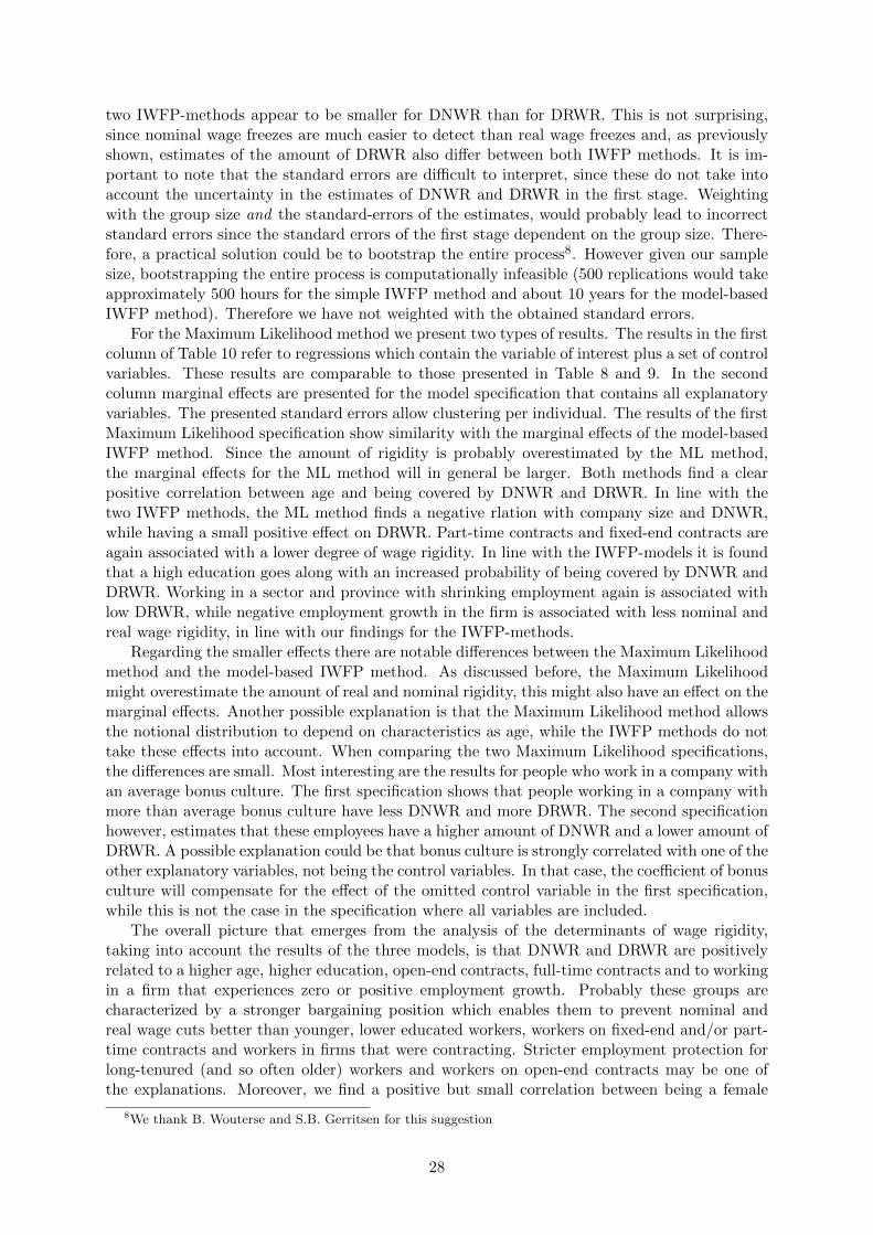
two IWFP-methods appear to be smaller for DNWR than for DRWR. This is not surprising,since nominal wage freezes are much easier to detect than real wage freezes and, as previouslyshown, estimates of the amount of DRWR also differ between both IWFP methods. It is im-portant to note that the standard errors are difficult to interpret, since these do not take intoaccount the uncertainty in the estimates of DNWR and DRWR in the first stage. Weightingwith the group size and the standard-errors of the estimates, would probably lead to incorrectstandard errors since the standard errors of the first stage dependent on the group size. There-fore, a practical solution could be to bootstrap the entire process8. However given our samplesize, bootstrapping the entire process is computationally infeasible (500 replications would takeapproximately 500 hours for the simple IWFP method and about 10 years for the model-basedIWFP method). Therefore we have not weighted with the obtained standard errors.

For the Maximum Likelihood method we present two types of results. The results in the firstcolumn of Table 10 refer to regressions which contain the variable of interest plus a set of controlvariables. These results are comparable to those presented in Table 8 and 9. In the secondcolumn marginal effects are presented for the model specification that contains all explanatoryvariables. The presented standard errors allow clustering per individual. The results of the firstMaximum Likelihood specification show similarity with the marginal effects of the model-basedIWFP method. Since the amount of rigidity is probably overestimated by the ML method,the marginal effects for the ML method will in general be larger. Both methods find a clearpositive correlation between age and being covered by DNWR and DRWR. In line with thetwo IWFP methods, the ML method finds a negative rlation with company size and DNWR,while having a small positive effect on DRWR. Part-time contracts and fixed-end contracts areagain associated with a lower degree of wage rigidity. In line with the IWFP-models it is foundthat a high education goes along with an increased probability of being covered by DNWR andDRWR. Working in a sector and province with shrinking employment again is associated withlow DRWR, while negative employment growth in the firm is associated with less nominal andreal wage rigidity, in line with our findings for the IWFP-methods.

Regarding the smaller effects there are notable differences between the Maximum Likelihoodmethod and the model-based IWFP method. As discussed before, the Maximum Likelihoodmight overestimate the amount of real and nominal rigidity, this might also have an effect on themarginal effects. Another possible explanation is that the Maximum Likelihood method allowsthe notional distribution to depend on characteristics as age, while the IWFP methods do nottake these effects into account. When comparing the two Maximum Likelihood specifications,the differences are small. Most interesting are the results for people who work in a company withan average bonus culture. The first specification shows that people working in a company withmore than average bonus culture have less DNWR and more DRWR. The second specificationhowever, estimates that these employees have a higher amount of DNWR and a lower amount ofDRWR. A possible explanation could be that bonus culture is strongly correlated with one of theother explanatory variables, not being the control variables. In that case, the coefficient of bonusculture will compensate for the effect of the omitted control variable in the first specification,while this is not the case in the specification where all variables are included.

The overall picture that emerges from the analysis of the determinants of wage rigidity,taking into account the results of the three models, is that DNWR and DRWR are positivelyrelated to a higher age, higher education, open-end contracts, full-time contracts and to workingin a firm that experiences zero or positive employment growth. Probably these groups arecharacterized by a stronger bargaining position which enables them to prevent nominal andreal wage cuts better than younger, lower educated workers, workers on fixed-end and/or part-time contracts and workers in firms that were contracting. Stricter employment protection forlong-tenured (and so often older) workers and workers on open-end contracts may be one ofthe explanations. Moreover, we find a positive but small correlation between being a female

8We thank B. Wouterse and S.B. Gerritsen for this suggestion

28

worker and wage rigidity. All three methods find that working in a large firm is related tohigher DNWR and lower DRWR. Large companies probably have more room to replace workersthat are reluctant to accept a nominal wage cut, while small companies might be dependenton specific skills of specific employees. Moreover, all three methods find that working in asector-province combination with shrinking employment is associated with lower DRWR. Thismight indicate that workers are to some extend willing to accept real wage cuts in favour ofemployment. Finally, a high wage is found to be positively related to both DNWR and DRWRaccording to the two IWFP-methods and to DNWR according to the ML-method. The factthat wages of 1− 2× modal income are nominally less rigid than the reference group that earnsless than the modal wage may be explained by lower wages following the statutory minimumwage, that is nominally rigid by definition in this period of observation. Other variables, forexample of the firms’ bonus culture and the country of origin of workers, generally show verysmall correlations.

Unfortunately, our data does not contain any information on the degree of organisation.Descriptive statistics on the degree of organisation, based on the (much smaller) Dutch LabourForce Survey Sociaal-economische Raad (2013) shows that the degree of organisation of employ-ees increases over age groups, over company size and is relatively high among full-time workersand workers on open-end contracts. The similarity between these highly organised groups andthe characteristics that are positively related to wage rigidity, suggests that being highly organ-ised may be an omitted variable that is behind the ability of these specific groups to preventwage cuts more successfully than other groups. All in all the results give the impression thatthe groups that are better protected and better organised have a higher ability to resist wagecuts. This contrasts with the finding by the OECD that “The slowdown in the growth rate ofearnings was fairly evenly spread across the earnings distribution” OECD (2014).

The fact that the three methods show similar correlations with worker and firm charac-teristics is an indication that all three methods measure the same phenomena. Although themethods do not agree on the amount of rigidity, they agree for a large part on what has apositive or negative relation with DNWR and DRWR. This implies that estimates of correla-tions between wage rigidity and worker and firm characteristics can be compared over countries.However, for the Maximum Likelihood method only estimates in a similar inflation environment(low or high) can be compared, since we did find indications that this method overestimatesthe amount of real and nominal rigidity in case of a low inflation environment. However, formeasuring the fraction of workers covered by DNWR ans DRWR, the choice of the method isimportant.

6 Conclusion

The three commonly used methods for estimating wage rigidity differ substantially with respectto their methodology, and as a consequence also with respect to the amount of rigidity theymeasure. A main challange in measuring wage rigidity is that the wage change distribution thatwould prevail in the absence of wage rigidity, the notional distribution, is unobserved. In themodel-based IWFP method it is assumed that the notional distribution is given by a two-sidedWeibull distribution. Deviations from this distribution are seen as rigidities. The MaximumLikelihood method however, assumes that wages are distributed normally without error anddeviations from this distribution are seen as rigidities.

One main finding is that the assumptions regarding the notional wage change distributionare an important determinant of the level of wage rigidity that is measured. We argue thatthe model-based IWFP approach is the preferred model of the three. First, the model based-approach has the most sophisticated method to take into account measurement error. Second,the model-based approach assumes that the notional distribution of wage changes is followsa two sided Weibull distribution, which is more realistic than a normally distributed notional

29

wage change distribution, as is assumed by the Maximum Likelihood approach. Based on bothour conceptional analysis and our empirical findings we argue that the normality assumptionin the Maximum Likelihood approach most probably leads to an overestimation of DRWR.A drawback of the simple IWFP approach is that the measurement of wage rigidity is verysensitive to the specified rate of inflation, since the estimation of the inflation expectation isnot incorperated in the model. Also, the simple model does not take into account measurementerrors.

As an additional analysis we study the correlation between wage rigidity as measured by thethree methods on the one hand and worker and firm characteristics on the other hand, using afractional logit model. We find coherent results: the presence of wage rigidity is unevenly dis-tributed among groups of workers: downward nominal and real wage rigidity in the Netherlandsare positively related to a higher age, higher education, open-end contracts, full-time contractsand to working in a firm that experiences zero or positive employment growth.

Hence, although the three methods do not agree on the amount of rigidity, they agree for alarge part on what variables have a positive or negative relation with downward nominal andreal wage rigidity. This is an indication that all three methods measure the same phenomenon,which implies that estimates of determinants of wage rigidity can be compared over countriesusing any of the three methods. However, for measuring the fraction of workers covered bydownward nominal or real wage rigidity, the choice of the method matters.

Besides, we contribute to the literature by providing accurate, internationally comparableestimates of wage rigidity in the Netherlands, based on administrative data. The only estimatesavailable so far for the Netherlands were based on survey data. The overall picture that wefind is that the Netherlands has a less than average amount of downward nominal wage rigiditycompared to other countries. However, for downward real wage rigidity the results of both ourpreferred model-based IWFP method and the Maximum Likelihood method point at a levelthat is above average compared internationally. DRWR is higher in Belgium (known for itsinflation compensation), France and Sweden, while Denmark, Italy, Germany, the UK and theUS show a substantially lower DRWR.

A limitation of this study is that it confines itself to wage rigidity among job stayers. Theliterature on displaced workers shows that dismissed workers in general earn lower wages intheir post-displacement jobs (Deelen et al., 2014).

Moreover, this study sheds no light on other mechanisms that are used by companies toadjust their costs in times of decreasing demand. A decomposition of how companies reducethe size of their wage bill, as done for Belgium in Fuss (2009), might give more insights inhow companies adapt to decreasing demand and might also give an indication of wage rigidity.Also this study does not go into the macroeconomic implications of wage rigidity. Evidence forstrong wage rigidity on the microeconomic level can be consistent with weak macroeconomiceffects (Lebow et al. (2003), Stuber and Beissinger (2012)). According to Elsby (2009), this canbe explained by forward looking behaviour of firms, that leads to compressed wage increases incase of downward wage rigidity.

Lastly our research did not focus on causal relations. Studying causes of wage rigidity isan interesting next step. This step, however, is challenging since it is difficult to come up withstrong instrumental variables.

References

Akerlof, G., Dickens, W., and Perry, G. (1996). The macroeconomics of low inflation. Brookingspapers on Economic Activity, 1996(1):1–76.

Akerlof, G., Dickens, W. T., and Perry, G. L. (2000). TD et Perry, GL 2000. Near-Rational

30

Wage and Price Setting and the Optimal Rates of Inflation and Unemployment. BrookingsPapers on Economic Activity.

Altonji, J. and Devereux, P. (2000). The extent and consequences of downward nominal wagerigidity. Research and Labor Economics, 19(Worker Well-Being):383–431.

Barwell, R. D. and Schweitzer, M. E. (2007). The Incidence of Nominal and Real Wage Rigiditiesin Great Britain: 1978-98. The Economic Journal, 117(524):F553–F569.

Bauer, T., Bonin, H., Goette, L., and Sunde, U. (2007). Real and Nominal Wage Rigiditiesand the Rate of Inflation: Evidence from West German Micro Data. The Economic Journal,117(524):F508–F529.

Behr, A. and Potter, U. (2010). Downward Wage Rigidity in Europe: A New Flexible ParametricApproach and Empirical Results. German Economic Review, 11(2):169–187.

Card, D. and Hyslop, D. (1997). Does Inflation ”Grease the Wheels of the Labor Market”? InReducing inflation: Motivation and strategy, pages 71–122. University of Chicago Press.

Deelen, A., De Graaf-Zijl, M., and Van den Berge, W. (2014). Labour market effects of jobdisplacement for prime-age and older workers. CPB Working Paper 285.

Devicienti, F., Maida, A., and Sestito, P. (2007). Downward Wage Rigidity in Italy: Micro-Based Measures and Implications. The Economic Journal, 117(524):F530–F552.

Dias, D., Marques, C., and Martins, F. (2013). The determinants of downward wage rigidity:some methodological considerations and new empirical evidence. Banco de Portugal EconomicBulletin, (Autumn 2013).

Dickens, W. and Goette, L. (2005). Estimating Wage Rigidity for the International WageFlexibility Project. mimeo, Brookings Institution, pages 1–20.

Dickens, W., Goette, L., Groshen, E. L., and Holden, S. (2007a). How Wages Change: MicroEvidence from the International Wage Flexibility Project. Journal of Economic Perspectives,21(2):195–214.

Dickens, W., Goette, L., Groshen, E. L., and Holden, S. (2007b). The interaction of labormarkets and inflation: Analysis of micro data from the International Wage Flexibility project.mimeo, Brookings Institution, pages 1–51.

Du Caju, P., Fuss, C., and Wintr, L. (2007). Downward Wage Rigidity for Different Workersand Firms: an evaluation for Belgium using the IWFP procedure. ECB Working Paper, 840.

Elsby, M. (2009). Evaluating the Economic Significance of Downward Nominal Wage Rigidity.Journal of Monetary Economics, 56(2):154–169.

Fehr, E. and Goette, L. (2005). Robustness and real consequences of nominal wage rigidity.Journal of Monetary Economics, 52(4):779–804.

Fouarge, D. and Baaijens, C. (2004). Changes of working hours and job mobility: the effect ofdutch legislation. OSA Working Paper, (23).

Fuss, C. (2009). What is the most flexible component of wage bill adjustment? Evidence fromBelgium. Labour Economics, 16(3):320–329.

Goette, L., Sunde, U., and Bauer, T. (2007). Wage Rigidity: Measurement, Causes and Conse-quences. The Economic Journal, 117(524):F499–F507.

31

Gottschalk, P. (2005). Downward nominal-wage flexibility: real or measurement error? Reviewof Economics and Statistics, pages 556–568.

Holden, S. and Wulfsberg, F. (2014). Wage Rigidity, Inflation, and Institutions. The Scandina-vian Journal of Economics, 116(2):539–569.

Kahn, S. (1997). Evidence of nominal wage stickiness from microdata. The American EconomicReview, 87(5):993–1008.

Katay, G. (2011). Downward wage rigidity in Hungary. ECB Working Paper, 1372.

Knoppik, C. and Beissinger, T. (2009). Downward nominal wage rigidity in Europe: an analysisof European micro data from the ECHP 1994-2001. Empirical Economics, 36(2):321–338.

Knoppik, C., C. (2007). The kernel-location approach - a new non-parametric approach to theanalysis of downward nominal wage rigidity in micro data. Economic Letters, 97(3):253–259.

Lebow, D. E., Saks, R. E., and Wilson, B. A. (2003). Downward Nominal Wage Rigidity:Evidence from the Employment Cost Index. Advances in Macroeconomics, 3(1).

Lunnemann, P. and Wintr, L. (2010). Downward wage rigidity and automatic wage indexation:Evidence from monthly micro wage data. ECB Working Paper, 1269.

McLaughlin, K. (1994). Rigid wages? Journal of Monetary Economics, 34(3):383–414.

Messina, J., Duarte, C., Izquierdo, M., Du Caju, P., and Hansen, N. (2010). The Incidenceof Nominal and Real Wage Rigidity: An individual-based sectoral approach. Journal of theEuropean Economic Association, 8(May 2010):487–496.

OECD (2014). Sharing the pain equally ? Wage adjustments during the crisis and recovery. InOECD Employment Outlook 2014. OECD Publishing.

Sociaal-economische Raad (2013). Verbreding draagvlak cao-afspraken.

Stuber, H. and Beissinger, T. (2012). Does Downward Nominal Wage Rigidity Dampen WageIncreases? European Economic Review, 56(4):870–887.

Tobin, J. (1972). Inflation and Unemployment. American Economic Review, 62:1–18.

32

Appendix

Table 11: Descriptive statistics of the observed wage change distributions for specific groups

(a) Male

Year N Mean Median Skewness Kurtosis SD do < 0 do < πML do < πCEP

2007 2469609 0.050 0.032 1.677 158.119 0.204 14% 34% 24%2008 2486712 0.057 0.042 3.357 152.439 0.189 11% 32% 31%2009 2529670 0.035 0.029 2.726 177.296 0.182 17% 42% 29%2010 2520213 0.027 0.013 3.977 199.673 0.185 18% 46% 51%2011 2477115 0.031 0.022 1.584 192.209 0.163 16% 39% 48%2012 2342712 0.029 0.022 0.018 222.487 0.173 17% 43% 47%

(b) Female

Year N Mean Median Skewness Kurtosis SD do < 0 do < πML do < πCEP

2007 1962319 0.058 0.038 2.420 73.990 0.247 19% 33% 26%2008 2003173 0.059 0.042 1.051 88.426 0.238 19% 36% 35%2009 2079537 0.042 0.030 0.702 110.324 0.231 23% 43% 32%2010 2132670 0.032 0.019 1.228 114.829 0.228 23% 43% 47%2011 2149168 0.034 0.020 0.859 101.443 0.212 24% 43% 50%2012 2045761 0.037 0.025 0.346 108.260 0.205 21% 42% 45%

(c) Full-time

Year N Mean Median Skewness Kurtosis SD do < 0 do < πML do < πCEP

2007 2687566 0.058 0.036 2.638 175.582 0.195 12% 31% 22%2008 2688527 0.064 0.045 4.417 180.321 0.178 10% 30% 29%2009 2718152 0.043 0.030 3.173 223.058 0.167 15% 39% 27%2010 2640252 0.034 0.016 5.111 245.025 0.171 16% 42% 47%2011 2582044 0.039 0.023 2.677 244.535 0.150 14% 36% 45%2012 2552386 0.037 0.024 1.930 263.409 0.151 15% 40% 43%

(d) Part-time

Year N Mean Median Skewness Kurtosis SD do < 0 do < πML do < πCEP

2007 1744362 0.047 0.031 1.763 64.760 0.263 23% 37% 30%2008 1801358 0.048 0.036 0.679 74.574 0.256 22% 40% 39%2009 1891055 0.032 0.026 0.709 90.129 0.251 27% 46% 36%2010 2012631 0.023 0.013 0.983 97.842 0.244 27% 48% 51%2011 2044239 0.024 0.016 0.548 86.258 0.225 27% 47% 54%2012 1836087 0.028 0.021 -0.418 97.176 0.231 25% 46% 49%

Source: own calculations based on Statistics Netherlands microdata

33