
Downward Nominal Wage Rigidities Bend the … Nominal Wage Rigidities Bend the Phillips Curve MARY...
52
FEDERAL RESERVE BANK OF SAN FRANCISCO WORKING PAPER SERIES Downward Nominal Wage Rigidities Bend the Phillips Curve Mary C. Daly Federal Reserve Bank of San Francisco Bart Hobijn Federal Reserve Bank of San Francisco, VU University Amsterdam and Tinbergen Institute January 2014 The views in this paper are solely the responsibility of the authors and should not be interpreted as reflecting the views of the Federal Reserve Bank of San Francisco or the Board of Governors of the Federal Reserve System. Working Paper 2013-08 http://www.frbsf.org/publications/economics/papers/2013/wp2013-08.pdf
Transcript of Downward Nominal Wage Rigidities Bend the … Nominal Wage Rigidities Bend the Phillips Curve MARY...

FEDERAL RESERVE BANK OF SAN FRANCISCO
WORKING PAPER SERIES
Downward Nominal Wage Rigidities Bend the Phillips Curve
Mary C. Daly Federal Reserve Bank of San Francisco
Bart Hobijn
Federal Reserve Bank of San Francisco, VU University Amsterdam and Tinbergen Institute
January 2014
The views in this paper are solely the responsibility of the authors and should not be interpreted as reflecting the views of the Federal Reserve Bank of San Francisco or the Board of Governors of the Federal Reserve System.
Working Paper 2013-08 http://www.frbsf.org/publications/economics/papers/2013/wp2013-08.pdf

Downward Nominal Wage Rigidities
Bend the Phillips Curve
MARY C. DALY BART HOBIJN
FEDERAL RESERVE BANK OF SAN FRANCISCO FEDERAL RESERVE BANK OF SAN FRANCISCO1
VU UNIVERSITY AMSTERDAM,
AND TINBERGEN INSTITUTE
January 11, 2014.
We introduce a model of monetary policy with downward nominal wage rigidities
and show that both the slope and curvature of the Phillips curve depend on the level
of inflation and the extent of downward nominal wage rigidities. This is true for the
both the long-run and the short-run Phillips curve. Comparing simulation results
from the model with data on U.S. wage patterns, we show that downward nominal
wage rigidities likely have played a role in shaping the dynamics of unemployment
and wage growth during the last three recessions and subsequent recoveries.
Keywords: Downward nominal wage rigidities, monetary policy, Phillips curve.
JEL-codes: E52, E24, J3.
1 We are grateful to Mike Elsby, Sylvain Leduc, Zheng Liu, and Glenn Rudebusch, as well as seminar participants at EIEF, the
London School of Economics, Norges Bank, UC Santa Cruz, and the University of Edinburgh for their suggestions and comments.
The original version of this paper was prepared for the conference on “Fulfilling the Full Employment Mandate,” on April 12-13,
2013, at the Boston Fed. The views expressed in this paper solely reflect those of the authors and not necessarily those of the
Federal Reserve Bank of San Francisco, nor those of the Federal Reserve System as a whole. Corresponding author: Bart Hobijn:

DALY AND HOBIJN
2
1. Introduction
Individual-level data on wage changes as well as survey-based evidence on wage setting show that
nominal cuts to pay are rare, suggesting that wages are downwardly rigid.2 Tobin (1972) argued that
such downward nominal wage rigidities induce a long-run, or steady-state, trade-off between
inflation and unemployment. Subsequent theoretical studies have formalized Tobin’s argument in
the context of a long-run Phillips curve that plots average inflation against the average
unemployment rate.3,4
The key finding from this work is that the long-run Phillips curve is nearly
vertical at high inflation and flattens out at low inflation, implying progressively larger output costs
of reducing inflation. However, even at low inflation, the long-run trade-off is not very big, at least
for levels of downward wage rigidities commonly observed in the U.S. (Akerlof, Dickens, and
Perry, 1996, Benigno and Ricci, 2011).
In this paper we add to this literature by considering how downward nominal wage rigidities
affect the short-run Phillips curve.5 Phillips (1958) documented significant curvature in the
historical relationship between money wage growth and unemployment in the U.K. He conjectured
that this curvature owed to the fact that “…workers are reluctant to offer their services at less than
prevailing rates when the demand for labour is low and unemployment is high so that wage rates
fall only very slowly.”6 Here we revisit Phillips’ hypothesis that downward nominal wage rigidities
bend the Phillips curve and in so doing we make both an empirical and theoretical contribution to
the literature.
We begin on the empirical side where we use micro data on wages from the Current Population
Survey (1986-2011) to document the existence of downward nominal wage rigidities in the United
2 For individual-level evidence for the U.S. see Akerlof, Dickens, and Perry (1996), Kahn (1997), Card and Hyslop (1997), Altonji
and Devereux (2000), Lebow, Saks, and Wilson (2003), Elsby (2009), Daly, Hobijn, and Lucking (2012). Individual-level
evidence for a large number of countries is in Dickens et al. (2007). Kahnemann, Knetsch, and Thaler (1986) and Bewley (1995,
1999) provide extensive anecdotal and survey evidence on downward nominal wage rigidities in the U.S. Bonin and
Radowski (2011) present survey results from Germany. Holden and Wulfsberg (2008) provide evidence from industry-level data. 3 Examples of such studies are Akerlof, Dickens, and Perry (1996), Kim and Ruge-Murcia (2008), Fagan and Messina (2009),
Benigno and Ricci (2011), Coibion et al. (2012). 4 Ball (1994) provides cross-country evidence on how the shape of the output-inflation trade-off depends on wage flexibility. 5 We define long-run as the steady state and short-run as deviations from the steady state. In the empirical work, this distinction
denotes plots of average inflation and the average unemployment rate (long-run) versus measured actual inflation and actual
unemployment (short-run). 6 Samuelson and Solow (1960) replicated Phillips’ results for the U.S. and found a similar curvature in the U.S. (wage) Phillips
curve. However, they argued the curvature might reflect an increase in the natural rate of unemployment rather than a bending due
to downward nominal wage rigidities. For the most part this latter view has been the consensus in modern macro models.

DOWNWARD NOMINAL WAGE RIGIDITIES
BEND THE PHILLIPS CURVE
3
States. We show that these rigidities rise substantially in recessions and remain elevated well after
the unemployment rate comes down. As we point out, this pattern for nominal wage rigidities
coincides with substantial curvature in the U.S. short-run Phillips curve. Specifically, during the
last three recession/recoveries plots of the Phillips curve show that unemployment first rose
significantly while wage growth remained flat and subsequently fell while wage growth decelerated.
To understand the coincidence of these two facts, the cyclical increase in downward nominal
wage rigidities and the bending of the short-run Phillips curve, we employ a dynamic general
equilibrium model of downward nominal wage rigidities and monetary policy, similar to those of
Benigno and Ricci (2011) and Fagan and Messina (2009). Our main contribution relative to these
authors is to solve for the full non-linear transitional dynamics of the model in response to demand
and supply shocks, taking into account the evolution of the distribution of wages along the
equilibrium path. Although previous studies have simulated the short-run Phillips curve (e.g.,
Benigno and Ricci), we are the first to focus on the joint cyclical path of unemployment and wage
growth following business cycle downturns.
The results highlight the importance of our approach. Our model generates the key patterns
highlighted in the data, namely the increase in downward nominal wage rigidities following
recessions and the subsequent bending of the short-run Phillips curve. Importantly, these results
hold for relatively conservative parameter values that generate fewer downward nominal wage
rigidities than measured in U.S. data.
Overall, the model simulations show that downward nominal wage rigidities bend the Phillips
curve in two ways. First, during recessions the rigidities become more binding and the labor market
adjustment disproportionately happens through the unemployment margin rather than through
wages. The higher the level of downward nominal wage rigidities the more this mechanism matters
and the higher the short-run sacrifice ratio between unemployment and inflation. Second, downward
nominal wage rigidities cause recessions to result in substantial pent up wage deflation. This leads
to a simultaneous deceleration of wage inflation and a decline in the unemployment rate during the
ensuing recovery period. This bending of the Phillips curve is especially pronounced in a low
inflationary environment.

DALY AND HOBIJN
4
We interpret our empirical work and model simulations as evidence that downward nominal
wage rigidities are an important force that has shaped the dynamics of unemployment, wage
growth, and inflation during and after the last three U.S. recessions.
The remainder of this paper is structured as follows. In Section 2 we present an update of
previous evidence on downward nominal wage rigidities in the U.S. and construct the U.S. wage
Phillips curve for 1986-2012. In Section 3 we describe our model of downward nominal wage
rigidities and monetary policy. In Section 4 we present numerical results for the steady state and
solve the transitional dynamics of the model. We conclude in Section 5.
2. Downward nominal wage rigidities and the U.S. wage Phillips curve
We begin by documenting the existence and importance of downward nominal wage rigidities in
the U.S. as well as the dynamics of unemployment and wage growth, as captured by the wage
Phillips curve. We use this evidence to establish several stylized facts about downward nominal
wage rigidities, the dynamics of wage growth, and unemployment in the U.S. during the period
1986-2012. We subsequently compare these facts to the transitional dynamics of our model of
downward nominal wage rigidities and monetary policy.
Empirical studies documenting the existence of downward nominal wage rigidities in the U.S.
emphasize that plots of the distribution of individual log wage changes display a prominent spike at
zero. We update this work in Figure 1. Following Card and Hyslop (1997), we track 12-month log
changes in the nominal wages of individuals using micro data from the Current Population Survey
(CPS).7 The histogram plots the distribution of wage changes in the CPS data for 2006 and 2011,
reflecting the distributions in two different points in the business cycle. We take the distribution of
wage changes in 2006 to represent the steady-state distribution and the distribution in 2011 to
represent the additional distortions that arise in business cycle downturns.8
7 Earlier studies (Akerlof, Dickens, and Perry, 1996, Kahn, 1997, Altonji and Devereux, 2000, and Elsby, 2009) used data from the
PSID for this type of analysis. However, the PSID has gone from an annual to a biannual frequency and thus does not allow for the
analysis of 12-month wage changes anymore. Another data source that would allow for a similar analysis is the Survey of Income
and Program Participation (SIPP). In results not shown we replicated our analysis using the SIPP. The key results were
qualitatively similar to those for the CPS although the prevalence of nominal rigidities is higher in the SIPP than in the CPS (see
Barattieri, Basu, and Gottschalk (2010) and Gottshalk (2005) for analyses of nominal wage rigidities using the SIPP). 8 Most studies of downward nominal wage rigidities focus on the wage changes of those who remain in the same job. Since our
model does not distinguish between job stayers and job switchers, we present the evidence for all workers who earned a wage at

DOWNWARD NOMINAL WAGE RIGIDITIES
BEND THE PHILLIPS CURVE
5
As the histograms in Figure 1 show, actual wage changes exhibit considerable discontinuity
with a prominent spike at zero. This is true in both 2006 and 2011. Consistent with the view that
individuals do not like nominal wage cuts (Kahneman et al. 1986, Bewley 1995,1999), the spike at
zero is produced asymmetrically, with most of the mass coming from the left of zero rather than
from the right. This suggests that a sizeable fraction of desired negative wage changes are being
swept up to zero (Altonji and Devereux 2000; Card and Hyslop 1996; Kahn 1997; Lebow, Saks,
Wilson 2003).
When we compare the 2006 histogram with that for 2011, three things stand out. First, the
fraction of workers with no wage change increased substantially in 2011 relative to 2006. In 2006
about 12 percent of workers reported zero wage change; in 2011 the share had risen to about 16
percent. Second, the fraction of workers getting a wage increase declined noticeably over the period
and the size of wage increases, conditional on getting one, was substantially lower in 2011 than in
2006. Thus, there is notable compression of wage gains near zero, suggesting that the inability to
adjust nominal wages downward may influence the magnitude of wage increases. This is a point
made by Elsby (2009). Finally and surprisingly, there is little difference in the fraction of workers
that get wage cuts between 2006 and 2011.
Another important stylized fact, hinted at in Figure 1, is that the prevalence of zero wage
changes varies over the business cycle. This can be seen in Figure 2 which plots the 12-month
moving average of the fraction of workers in the CPS data reporting zero nominal wage changes
along with the unemployment rate. As the figure shows, there is always a non-trivial fraction of
workers receiving zero wage changes in the U.S. economy. This fraction increases around business
cycle downturns although with a lag relative to the unemployment rate. These two patterns: (i) the
spike at zero wage changes lags the spike in the unemployment rate, and (ii) the prevalence of zero
wage changes stays high well after the unemployment rate has begun to come down are two
features of the data that Phillips (1958) argued could produce curvature in the wage Phillips curve.
To see if such curvature is present in the U.S. data, Figure 3 plots the wage Phillips curve for the
U.S. using measures of the nominal wage growth gap and unemployment gap for 1986 through
2012. The nominal wage growth gap is the percentage point difference between a composite
the beginning and end of the year. However, in other work we show that although downward nominal wage rigidities are higher
for job stayers, they also are present for job changers (see: http://www.frbsf.org/economic-research/nominal-wage-rigidity).
DALY AND HOBIJN
6
measure of wage growth and 10yr-ahead inflation expectations from the Survey of Professional
Forecasters. We use it to capture cyclical fluctuations in nominal wage growth rather than those due
to shifts in long run inflation expectations. The composite measure of wage growth we use is the
first principal component of the four major wage series for the U.S.9 The unemployment gap is
defined as the percentage point difference between the civilian unemployment rate and the long-
term natural rate of unemployment, as estimated by the Congressional Budget Office. For ease of
comparison we separately plot the three recession and recovery periods in our sample. Observations
for each of these three episodes are connected by arrows. The other quarters are plotted as gray
points.
Figure 3 shows the expected (Phillips, 1958, Solow and Samuelson, 1960, Galí, 2011)
relationship between wage growth and labor market slack; higher slack means slower wage growth,
lower slack means faster wage growth. The figure also shows distinct non-linearities in the curve in
the three recession/recovery periods in our sample. These nonlinearities highlight the fact that as
slack increases during recessions, wage growth slows but not nearly as much as a linear model
would predict. As the labor market recovery begins and the unemployment rate falls, the reverse
occurs As unemployment comes down, wage growth continues to decelerate. As we will show in
our model, these dynamics of wage growth and unemployment during the last three recessions and
recoveries are consistent with downward nominal wage rigidities preventing wage adjustments so as
to bend the short-run Phillips curve.10
In the next section we describe our model of monetary policy with downward nominal wage
rigidities. Solving the short-run transitional dynamics of this model we examine whether we can
qualitatively match the empirical patterns just discussed including the spike at zero in no wage
changes, the lag in the spike at zero of wage changes relative to the unemployment rate, and the
bending of the Phillips curve that occurs in recessions and recoveries.
9 Appendix B contains a brief description of how this composite measure is constructed. 10 Although the prevalence of downward nominal wage rigidities and the bending of the Phillips curve are most striking for the Great
Recession, the fact that it these patterns also emerged in the two previous recessions suggest that the dynamic we focus on is not
due to circumstances that are specific to the 2007 recession, like monetary policy hitting the zero lower bound.
DOWNWARD NOMINAL WAGE RIGIDITIES
BEND THE PHILLIPS CURVE
7
3. Model of monetary policy with DNWR
We employ a simple discrete-time model, similar to those of Benigno and Ricci (2011) and Fagan
and Messina (2009). Our main contribution relative to these authors is to solve for the full non-
linear transitional dynamics of the model in response to demand and supply shocks, taking into
account the evolution of the distribution of wages along the equilibrium path. Although previous
studies have simulated the short-run Phillips curve (e.g., Benigno and Ricci, 2011), we are the first
to focus on the joint cyclical path of unemployment and wage growth following business cycle
downturns. Throughout this section we point out where our model differs from those used in
previous studies, either (i) to keep the model tractable such that we can solve for its transitional
dynamics, or (ii) to use more general and realistic functional forms, like for the monetary policy
rule.
Firms
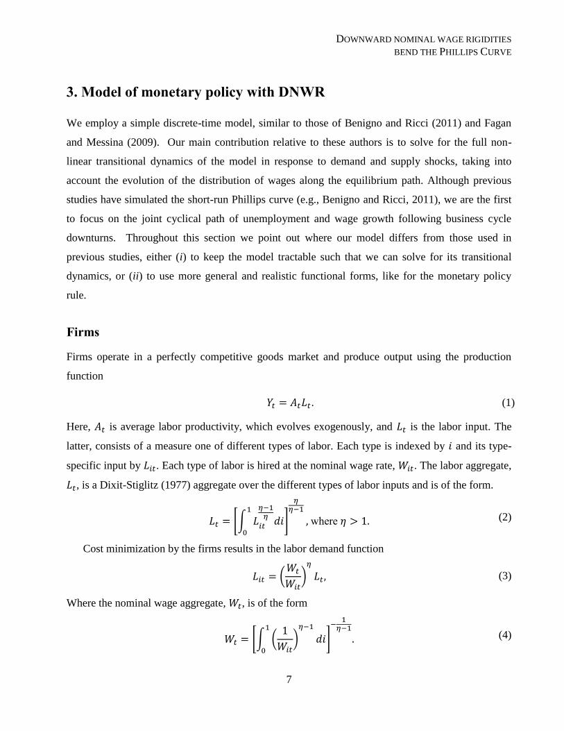
Firms operate in a perfectly competitive goods market and produce output using the production
function
. (1)
Here, is average labor productivity, which evolves exogenously, and is the labor input. The
latter, consists of a measure one of different types of labor. Each type is indexed by and its type-
specific input by . Each type of labor is hired at the nominal wage rate, . The labor aggregate,
, is a Dixit-Stiglitz (1977) aggregate over the different types of labor inputs and is of the form.
[∫
]
where (2)
Cost minimization by the firms results in the labor demand function
(
)
(3)
Where the nominal wage aggregate, , is of the form
[∫ (
)
]
(4)

DALY AND HOBIJN
8
Because firms operate in a perfectly competitive goods market, the equilibrium price level, ,
equals the unit production cost, ⁄ . Thus, equilibrium in the goods market implies that the
detrended real wage aggregate in this economy is constant and equal to one. That is,
[∫ (
)
]
[∫ (
)
]
(5)
Here, ⁄ is the detrended real wage rate of labor of type at time . Moreover, perfect
competition implies that costs exhaust revenue and that there are thus no profits and markups that
could contribute to the wedge between wage and price inflation.11
The only factor that contributes
to this wedge is the exogenous productivity growth rate,
.
Households
We follow Fagan and Messina (2009) and Benigno and Ricci (2011) and model downward nominal
wage rigidities based on the staggered wage setting model of Erceg, Henderson, and Levin (2000).
That is, we consider a representative household in which the members share their consumption risk
and individually set the wage they charge for their labor services. They then supply as much labor
as is demanded by the firms.
The representative household chooses its path of consumption, ,12
and wages and labor supply
{ }
to maximize the present discounted value of the stream of utility
∑ ∑
{
∫
}
where (6)
Here is the disutility from working for household member , which varies over time; is a
“shock” that affects the household’s discount factor.13
The household maximizes this objective
function subject to five constraints.
11 Most New Keynesian models with price stickiness have countercyclical markups (e.g. Galí and Gertler, 1999) . Though, recent
empirical estimates by Nekarda and Ramey (2010) suggest that markups might actually be procyclical. 12 The absence of capital goods in the economy means that, in equilibrium, output, , equals the level of consumption of the
representative household, . Throughout this paper, we substitute in this equilibrium condition and use . 13 We put “shock” here in quotation marks because we assume that the household knows the path { }
. In addition, we assume
that in the long run is zero.

DOWNWARD NOMINAL WAGE RIGIDITIES
BEND THE PHILLIPS CURVE
9
The first is the budget constraint. Defining the level of nominal assets held by the household at
the end of period as and the nominal interest paid during period on the assets held at the end
of period as , we write this constraint as
( ) ∫
(7)
The second constraint is that each of the members of the household sets their wage taking as
given the labor demand function in equation (3). Given that in equilibrium the aggregate detrended
real wage equals one, this labor demand function can be written in terms of the real wage charged
by household member as
(
)
(8)
The third constraint is that, because every household is infinitesimally small, it takes as given
the path of the aggregate wage, , and labor input, , the price level, , and the nominal interest
rate, .
The fourth constraint is that the household takes the path of its discount rate shock, ,
productivity growth, , as well as the stochastic process that drives the member-specific disutility
of working, , as given. In particular, we assume that in each period a member’s disutility from
working is drawn from a log-normal distribution, where ( ) (
) such that [ ] .
14
This means that there is no persistence in the disutility shocks, . We make this assumption to
keep the equilibrium dynamics of the model tractable and solvable.
The final constraint is that of downward nominal wage rigidities. Similar to Fagan and Messina
(2009), we model these rigidities along the lines of the time-dependent price stickiness of
Calvo (1983) commonly used in models with price rigidities. In particular, we assume that, every
period, a randomly selected fraction [ ) of household members is not allowed to change their
nominal wage downward and have to set their wage subject to the constraint .15
14 Our setup with disutility shocks follows Benigno and Ricci (2011). Alternatively, one can introduce household member specific
productivity shocks, as in Fagan and Messina (2009). Both these approaches lead to similar equilibrium dynamics. The latter,
however, results in a more complicated expression for the aggregates in equilibrium. To keep our illustrative model as simple as
possible, we chose the former. Some technical details about the log-normal distribution, which we use for our derivations, are
described in Appendix A. 15 In terms of the notation in Fagan and Messina (2009, equation 17), we assume that , and . Their probability
is in our notation.

DALY AND HOBIJN
10
Optimal savings decision
Defining the inflation rate as , the household’s saving decision yields the Euler equation
( )
(9)
where is the real interest rate and is given by ( ) ( )⁄ . Since our model
economy does not exhibit any aggregate uncertainty, there is no uncertainty about future inflation,
.
Wage setting under flexible wages: .
Similar to Erceg, Henderson, and Levin (2000) and Benigno and Ricci (2011), each household
member chooses the sequence of detrended real wages, , to maximize the expected present value
of the difference between the utility value of the generated labor income and the disutility from
providing the labor services demanded by firms.
As we show in Appendix A, this reduces to the household choosing the path of wages of
member to maximize
[∑ ∑
( )
] (10)
where
( )
[
]
(11)
Note that the objective here is an expected present discounted value because, even though the
household as a whole does not face any aggregate uncertainty, each individual member of the
household faces uncertainty about the future path of the idiosyncratic shocks to its disutility from
working, .
When wages can be flexibly adjusted then, in every period, the real wage is chosen to
maximize ( ). The resulting optimal detrended real wage schedule is
( ) (
)
(12)
This turns out to be an important benchmark to compare the wage-setting under downward nominal
wage rigidities to.

DOWNWARD NOMINAL WAGE RIGIDITIES
BEND THE PHILLIPS CURVE
11
Wage setting under downward nominal wage rigidities: .
When household members’ wage setting choices are subject to downward nominal wage rigidities,
their decisions depend on and , as well as the future path of these aggregates, the future path
of inflation, , the path of productivity growth, , and the demand shock, . Two things produce
this dependency. First, each of these variables influences the likelihood that a household member
will want to reduce the current wage at some point in the future. Second, together these variables
determine the present discounted value associated with the potential inability to cut wages in future
periods.
In order to formalize the optimal wage setting problem under downward nominal wage
rigidities, we define the value of the objective (10) for a household member who gets paid a
detrended real wage at the beginning of period as ( ). We then hit this worker with a
disutility shock, i.e. a draw of a value of , after which the worker decides whether and how to
change the charged detrended real wage, .
With probability ( ) the worker is able to choose any non-negative wage desired in period
. With probability , the worker is restricted from choosing a detrended real wage smaller than .
In other words, the worker can set such that . Because of inflation and productivity
growth, once the worker has chosen a detrended real wage rate in period , the period real
wage is equal to [( )( )]⁄ .
The resulting optimization problem can be written in the form of the following Bellman
equation
( ) ( )∫
{ ( ) ( [( )( )]⁄ )} ( )
∫
{ ( ) ( [( )( )]⁄ )} ( )
(13)
Here, ( ) denotes the distribution function of the idiosyncratic preference shocks. We show in
Appendix A that all workers who are not constrained in their wage setting in period and have the
same disutility level, , choose the same detrended real wage ( ). Moreover, the wage they
set is strictly increasing in . This means that ( ) is invertible and we denote its inverse as
( ). This function gives the disutility from working value at which workers set their detrended
real wage to .

DALY AND HOBIJN
12
It is important to note that the existence of downward nominal wage rigidities affects the wage-
setting decisions of workers who do and do not face the constraint in the current period. For those
who face the constraint the statement is obvious. For those who do not face the constraint, the effect
works as follows. The wage that non-constrained workers set in the current period, , determines the
likelihood of being constrained in the next period. The higher the wage they set the higher this
probability. Thus, relative to the flexible wage-setting case, downward nominal wage rigidities add
an additional marginal cost to raising current wages. Consequently, such workers will set their wage
lower than or equal to what they would have done in the absence of DNWR, that is ( ) .
This is reminiscent of Elsby (2009) who emphasizes that downward nominal wage rigidities not
only prevent wage declines but they also dampen wage increases.
The workers who set a real wage and face the DNWR constraint in the current period consist
of two groups. The first group consists of those who get a shock, ( ), such that they would
like to increase their wage anyway and for whom the constraint is thus not binding. The second
group, for whom the constraint is binding, get a disutility shock such that the wage they currently
charge, , is higher than the wage they would have set under flexible wage setting, . We show in
Appendix A, that these workers will keep their wage fixed at .
Monetary policy rule
Because wages in this economy are sticky due to the downward nominal wage rigidities, there is
room for monetary policy to affect the allocation of resources in equilibrium. Since our emphasis in
this paper is not on optimal policy, but rather on the shape of the Phillips curve for a given
monetary policy rule, we assume that the central bank, which targets an inflation rate equal to ,
sets the nominal interest rate according to a standard Taylor (1993) rule.1617
That is, the central
bank’s policy rule is
( )( )
(
)
(
)
(14)
16 An obvious extension to our results would be to include a zero lower bound (ZLB) constraint on monetary policy accommodation.
However, as we showed in Figure 3, the bending of the wage Phillips curve that is the focus of our analysis also occurred in
recessions where the ZLB was not binding. 17 In Benigno and Ricci (2011) the central bank follows a nominal output target. We use the Taylor rule as a more realistic treatment
of central bank policy.

DOWNWARD NOMINAL WAGE RIGIDITIES
BEND THE PHILLIPS CURVE
13
Here, ⁄ is the level of output in deviation from trend, and is its associated steady-state
level, such that ⁄ is one plus the output gap. The steady-state level of productivity growth is .18
Equilibrium
Equilibrium in this economy is a path of { } that satisfies (i) the production
function, (1), (ii) the consumption Euler equation, (9), (iii) the Fisher equation, and (iv) the
monetary policy rule, (14). In addition, (v) the wage setting decisions satisfy that the real wage
equals 1, i.e. (5).
Under downward nominal wage rigidities the current wage setting by workers depends not only
on current economic conditions and their expectations of future economic outcomes but also on
their past wage-setting decisions. Thus, the distribution of real wages is a state variable that
determines the equilibrium dynamics of the economy. As a result, the equilibrium dynamics of this
economy cannot be solved in closed form and need to be simulated numerically. In this subsection
we describe the main recursive equations that drive these equilibrium dynamics. Before we do so,
however, we first consider the special case in which wages can be adjusted flexibly, .
Equilibrium under flexible wages, .
This is a useful benchmark for comparison since it can be solved analytically. Because there are no
nominal rigidities, the Classical Dichotomy holds and monetary policy does not affect the allocation
of goods and labor in the economy. We thus limit our analysis to the real equilibrium variables
under flexible wages.
As we show in Appendix A, when wages can adjust flexibly, the equilibrium level of the labor
input is given by
(
)
(
)
(15)
where
18 To cut back on notation, in the rest of our derivations, we use that ⁄ , and is the steady-state level of the labor
input.

DALY AND HOBIJN
14
[∫ (
)
( )
]
( )
( )
(16)
is the aggregate level of the disutility from working. The first factor on the right-hand side of
equation (15) reflects the output loss due to the workers charging a wage markup and setting their
wages inefficiently high. This reduces the equilibrium level of labor demanded and thus of output.
If the elasticity of substitution between the different types of labor, , goes to infinity then this
markup disappears and the equilibrium level of output under flexible wages coincides with that
obtained in the first-best where both the goods and labor markets are perfectly competitive.
Equilibrium under downward nominal wage rigidities, .
The equilibrium dynamics in the general case, where , depend on the evolution of the
distribution of real wages across workers. We denote the distribution of real wages in period after
each of the workers has set their wage by ( ) and the corresponding density function by ( ).
The evolution of this distribution function is driven by three types of workers.
Figure 4 illustrates these three groups. Consider those that end up with a real wage or lower
in period . There are three types of wage setters for whom this happens.
The first type consists of those who are not subject to the DNWR constraint in period and
draw a productivity shock, ( ), such that they would like to set their wage lower than or
equal to . In Figure 4 this a fraction ( ) of all household members in the areas , , and .
The share of workers in these areas is equal to ( ( )).
The second type is those workers who are subject to the DNWR constraint in period , started
the period at a detrended real wage , and drew a shock, ( ) ( ) that makes
them want to raise their detrended real wage to a level lower than or equal to . These workers
make up a fraction of those in the area in Figure 4. They are the ones with real wages lower or
equal to for which the DNWR constraint is not binding.
The final type of worker is those who are constrained by downward nominal wage rigidities.
These workers started the period with a detrended real wage and drew a shock ( ).
That is, they would like to lower their wage but are not able to. These individuals make up a
fraction of workers in the area in Figure 4.
DOWNWARD NOMINAL WAGE RIGIDITIES
BEND THE PHILLIPS CURVE
15
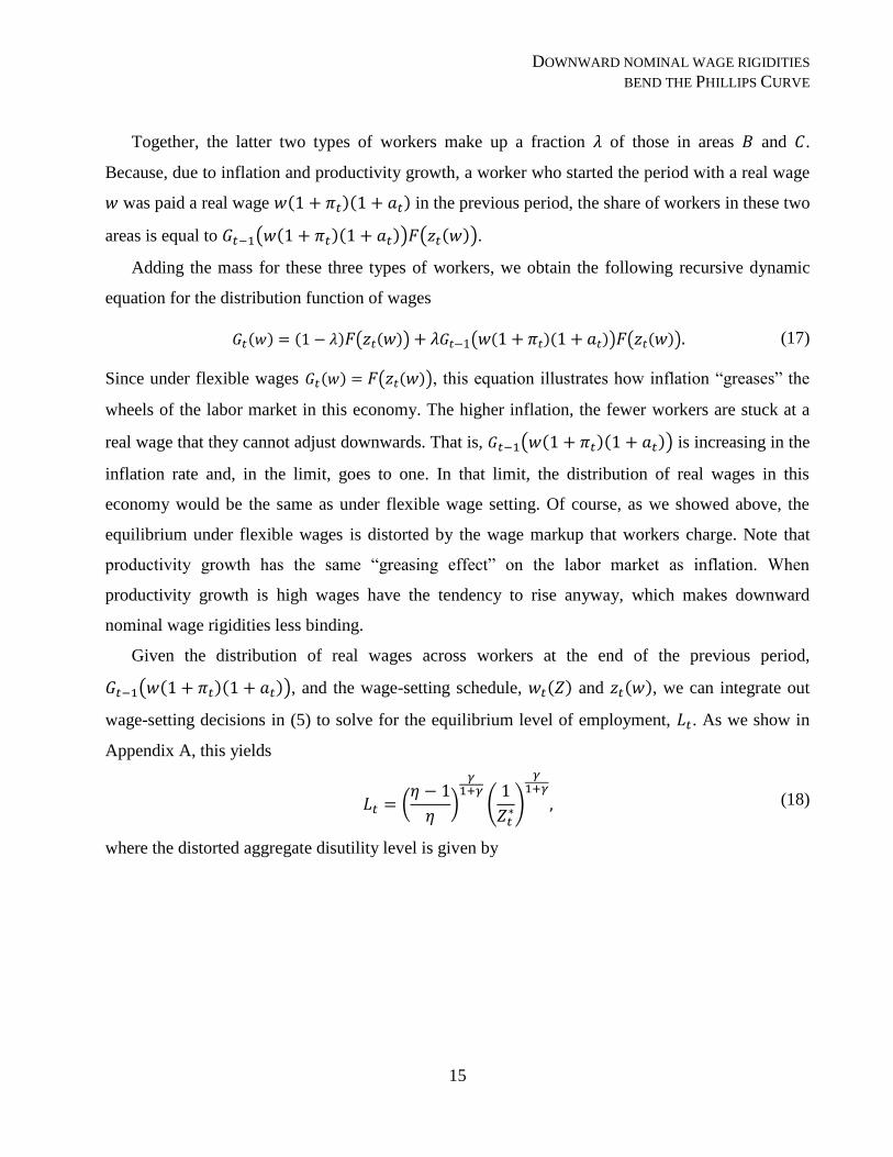
Together, the latter two types of workers make up a fraction of those in areas and .
Because, due to inflation and productivity growth, a worker who started the period with a real wage
was paid a real wage ( )( ) in the previous period, the share of workers in these two
areas is equal to ( ( )( )) ( ( )).
Adding the mass for these three types of workers, we obtain the following recursive dynamic
equation for the distribution function of wages
( ) ( ) ( ( )) ( ( )( )) ( ( )) (17)
Since under flexible wages ( ) ( ( )), this equation illustrates how inflation “greases” the
wheels of the labor market in this economy. The higher inflation, the fewer workers are stuck at a
real wage that they cannot adjust downwards. That is, ( ( )( )) is increasing in the
inflation rate and, in the limit, goes to one. In that limit, the distribution of real wages in this
economy would be the same as under flexible wage setting. Of course, as we showed above, the
equilibrium under flexible wages is distorted by the wage markup that workers charge. Note that
productivity growth has the same “greasing effect” on the labor market as inflation. When
productivity growth is high wages have the tendency to rise anyway, which makes downward
nominal wage rigidities less binding.
Given the distribution of real wages across workers at the end of the previous period,
( ( )( )), and the wage-setting schedule, ( ) and ( ), we can integrate out
wage-setting decisions in (5) to solve for the equilibrium level of employment, . As we show in
Appendix A, this yields
(
)
(
)
(18)
where the distorted aggregate disutility level is given by

DALY AND HOBIJN
16
{( )∫ (
)
( )
( ( )
( ))
( )
∫ (
)
( )
( ( )( )( )) ( ( )
( ))
( )
∫ (
)
( )
[∫ ( ) ( ( )( )) ( ( )
)
( )
] ( )
}
( )
(19)
Each of the three lines in this equation corresponds to a different type of worker. The third line
reflects the workers who are constrained by the downward nominal wage rigidities. These workers
are the reason that the level of employment is lower under downward nominal wage rigidities than
under flexible wages. They are stuck charging a wage higher than they initially intended because
they drew an unexpectedly low disutility shock, . Stuck at this wage, they end up providing fewer
labor services than they wanted to supply. The existence of the idiosyncratic shocks is thus a central
part of this argument. Without them, downward nominal wage rigidities are unlikely to cause a
substantial distortion in equilibrium. In fact, most studies of downward nominal wage rigidities
without such shocks find that very small effects on labor market allocations and welfare.19
Even with idiosyncratic shocks, the employment loss due to workers being stuck at a high wage
is partly offset by the change in wage setting behavior for the workers who do adjust their wage.
They make up the first two lines in equation (19). In order to decrease the likelihood of the
downward rigidities being binding in the future, they set their wage, ( ), lower than under
flexible wages, ( ). At this lower real wage they end up supplying more labor than they would
have under flexible wages. This is a point that Elsby (2009) emphasizes as limiting the welfare cost
of downward nominal wage rigidities.20
Comparing (18) with (15) one can see that the net effect of downward nominal wage rigidities is
captured by the ratio ⁄ . This is the labor wedge introduced by the rigidities. This labor wedge
results in a shortfall in employment in equilibrium relative to the economy under flexible wages.
Following Benigno and Ricci (2011) we define the unemployment rate, , in our model as the
19 See Kim and Ruge-Murcia (2008) and Coibion, Gorodnichenko, and Wieland (2012), for example. Carlsson and Westermark
(2008) even find that DNWR can be welfare improving because they reduce wage fluctuations. 20 Ball and Mankiw (1994) make a similar point about the welfare costs of asymmetric costs to price adjustments.

DOWNWARD NOMINAL WAGE RIGIDITIES
BEND THE PHILLIPS CURVE
17
percentage shortfall in employment under downward nominal wage rigidities compared to under
flexible wages.
How DNWR bend the Phillips curve
To understand how our model generates the type of bending of the wage Phillips curve evident in
the data in Figure 3 it is useful to interpret the time path of the wage Phillips curve as the result of
the changing intersection of an aggregate demand (AD) curve and a short-run aggregate supply
(SRAS) curve. Since the positions of both of these curves shift in response to shocks, the
intersection points change to produce a short-run time path of the wage Phillips curve.
In our model, the AD curve reflects the combinations of the unemployment rate, , and (wage)
inflation rate, , consistent with the combination of the monetary policy rule, (14), and
consumption Euler equation, (9). Since these two equations depend on current output they also
depend implicitly on the unemployment rate, inflation, as well as the discount rate shock, , the
productivity shock, , and the future path of the equilibrium variables. This means that the AD
curve moves in response to different shocks. For our main experiment of a negative discount rate
shock the curve shifts outward relative to the steady state.
The SRAS curve in our model is given by all combinations of the unemployment rate, , and
the inflation rate, , that satisfy (18), where all workers follow the optimal wage setting schedule
implied by the Bellman equation (13). This short-run aggregate supply curve is declining in the
inflation rate. This is because a decline in inflation makes DNWR bind for more workers who are
not able to reduce their wages. This reduces total labor demand and output relative to what it would
have been at the higher inflation rate and increases unemployment.
The SRAC curve also shifts out in response to our main shock—a negative discount rate shock,
. This is because such a shock increases the weight on the continuation value,
( ( )( )⁄ ), in equation (13), which is the effective marginal cost of pay
increases. This results in a compression of wage increases similar to that shown in Figure 1. But
when overall wage increases are compressed, the DNWR constraint binds for more workers and
results in a higher unemployment rate, shifting the SRAS curve outwards.
This means that in the presence of downward nominal wage rigidities a negative discount rate
shock acts both as a negative demand shock, that shifts the AD curve, and as a negative supply

DALY AND HOBIJN
18
shock, that shifts the SRAS curve. How this nets out to affect the short-run wage Phillips curve
depends on the relative movements in the AD and SRAS curves in response to the initial shock and
the relative movement of the two curves back to their pre-shock steady-state locations. Figure 5
illustrates two relevant cases, one for low rigidities and one for high rigidities. For context, note that
in the limiting case where wages are fully flexible the SRAS curve is vertical and does not shift in
response to the shock. In that case, which satisfies the Classical Dichotomy, a discount shock would
only affect the level of inflation and not output and the unemployment rate.
Moving slightly away from the limiting case, Panel (a) of Figure 5 shows how the AD and
SRAS curves respond to a negative discount rate shock when downward nominal wage rigidities are
low. Since we are not far from the flexible wages case, the SRAS does not move very much in
response to the shock; in the figure it moves from SRAS to SRAS’. In contrast, the AD curve
moves a lot. This results in a relatively low sacrifice ratio in response to the shock. After the shock,
the movements in the AD curve back to its original position are much larger than that of the SRAS
curve. These relative movements of the curves generate a subsequent path that displays the opposite
type of curvature than we observe in the data, illustrated by the curved dark line in the figure.
Considering a more realistic case based on the U.S. data, Panel (b) of Figure 5 shows what
happens when downward nominal wage rigidities are high. In that case the SRAS curve is flatter
and shifts out more in response to the shock. This results in a higher sacrifice ratio in response to
the shock. During the adjustment back to the steady state, the inward movement in the SRAS is
faster than that in the AD curve, resulting in the type of curvature in the wage Phillips curve that we
observe in the data in Figure 3.
The type of curvature observed in the data and the illustrative examples provided in Figure 5
suggest that downward nominal wage rigidities are relevant for the dynamics of wage growth and
the unemployment rate. In the next section, show how the equilibrium path of our model looks like
panel (b) of Figure 5. Unfortunately, neither the steady-state value nor the equilibrium path of our
model can be solved in closed form. Therefore, we use numerical examples in the next section to
illustrate how our model satisfies the main intuition captured in Figure 5.

DOWNWARD NOMINAL WAGE RIGIDITIES
BEND THE PHILLIPS CURVE
19
4. Numerical results
Steady state equilibrium
In this subsection we show that our model produces similar long-run properties to those emphasized
in other theoretical studies of downward nominal wage rigidities (Akerlof, Dickens, and Perry,
1996, Fagan and Messina, 2009, and Benigno and Ricci, 2011). Specifically, we show that in
steady-state, our model generates the familiar long-run trade-off between unemployment and
inflation due to downward nominal wage rigidities. We also show that our model produces the same
distortions in the distribution of nominal wage changes documented in micro studies and shown in
Figures 1 and 2. These include the spike at zero wage growth and the missing mass of negative and
positive wage changes associated with downward nominal wage rigidities.
Calibration of parameters that matter for the steady state
We split the parameters that matter for the steady-state outcome of our model into two groups. The
first consists of the basic preference and technology parameters which we choose based on previous
studies and historical evidence for the U.S. In particular, we follow Benigno and Ricci (2011) and
set the wage elasticity of labor demand to and the Frisch elasticity of the labor supply,
. We set trend productivity growth, , to match the 2.7 percent average annualized growth
rate of labor productivity from 2001 through 2007. Furthermore, we assume that the discount factor,
, is 2 percent annualized. In combination with the level of trend productivity growth, , this pins
down the natural real interest rate.21
Time, , is measured in quarters.
The second group contains the parameters that affect the importance of DNWR in equilibrium:
(i) , the probability of being subject to the downward nominal wage rigidities constraint in a
period, (ii) the variance of the idiosyncratic shocks, , and (iii) the target inflation level, , and
degree to which it greases the labor market in the sense of (17).22
Throughout the rest of this
subsection we investigate how changes in these parameters affect the steady-state unemployment
21 Since, in steady state, the inflation rate is equal to its target, , and the output gap is zero, the monetary policy parameters, and
do not affect the steady-state outcome. 22 In principle, the level of trend productivity growth, , also affects the degree of DNWR because trend productivity growth greases
the wheels of the labor market in the same way that inflation does. Because their effects are identical, we focus on variation in the
target inflation rate, .

DALY AND HOBIJN
20
rate and wage setting.23
We use as our benchmark-case and , which results in a 5
percent natural rate of unemployment at a 2 percent (annualized) inflation target. The benchmark
parameter values that we use are listed in Table 1.
Long-run Phillips curve
Figure 6 plots the long-run Phillips curves from our model for four different degrees of downward
nominal wage rigidities, { }. For we plot two curves, one for ,
solid line, and one for , dashed line. The benchmark-case and is denoted
by the thick black line in the figure. The vertical axis is the inflation target and the horizontal axis is
the natural rate of unemployment that results from the inflation-target choice.
Several points are worth noting in this figure. First, for all four degrees of rigidities, the long-run
Phillips curve is downward sloping. This is consistent with the idea that inflation greases the wheels
of the labor market, so that the lower the central bank’s inflation target the less lubricated the labor
market and the higher the natural rate of unemployment. Second, the long-run sacrifice ratio is
increasing in the degree to which the downward nominal wage rigidities are binding. In other
words, as increases, unemployment increases for a given reduction in the target inflation rate. Of
course, our model solely focuses on downward nominal wage rigidities. A more general analysis of
the optimal inflation target, like and Coibion, Gorodnichenko, and Wieland (2012), would take into
account the many different costs and benefits of (steady-state) inflation (see, Fischer and
Modigliani, 1978).
A third point worth noting is that changes in , illustrated for , produce two effects.
Higher values of increase the degree to which downward nominal wage rigidities are binding,
pushing the long-run Phillips curve out. Raising also alters the slope of the long-run Phillips
curve, albeit slightly, with very little impact on the sacrifice ratio.
Our results are similar to those from previous research. For example, the average long-run
sacrifice ratio for are of a similar magnitude as that in Akerlof, Dickens, and Perry (1996,
Figure 3) in that an increase of the inflation target from 0 to 10 results in an approximately 3
percentage point drop in the natural rate of unemployment. And like Akerlof, Dickens, and Perry
23 We interpret the steady-state unemployment rate as the natural rate of unemployment in the rest of this paper.

DOWNWARD NOMINAL WAGE RIGIDITIES
BEND THE PHILLIPS CURVE
21
(1996, Figure 3) and Benigno and Ricci (2011, Figure 2), we find that the long-run Phillips curve is
bent such that the long-run sacrifice ratio is higher for lower target inflation rates.
Distortion of log nominal wage changes
The long-run unemployment-inflation trade-off that downward nominal wage rigidities induce is the
result of the rigidities distorting wage-setting behavior. To illustrate this distortion, we plot the
theoretical equivalent of the distribution of log nominal wage changes, depicted in Figure 1, for
percent (annualized) and for as well as for the case of flexible wages, . The
distribution of quarterly log nominal wage changes in our model is plotted in Figure 7.
Log-normality of the idiosyncratic shocks, , together with the optimal wage setting under
flexible wages, (12), implies that, under flexible wages, the steady-state distribution of quarterly log
nominal wage changes will be normal with a mean equal to the sum of the quarterly steady-state
inflation rate, in this case 0.5 percent, and productivity growth, which we set at 0.66 percent. This is
the ‘flexible’ distribution plotted in Figure 7.
The distribution of quarterly log wage changes under downward nominal wage rigidities looks
notably different. As we documented in the empirical section, the presence of downward nominal
wage rigidities distorts this distribution in three ways. First, there are many fewer negative wage
changes due to the rigidities. Second, the rigidities result in a spike at zero nominal wage changes.
For our parameter combination, 57 percent of workers have the same wage as in the previous
quarter. Third, and most surprisingly, there are many fewer positive wage changes and those that do
occur are smaller than under flexible wages.24
In our model, under flexible wages 56 percent of
workers get a quarterly wage increase of 0.25 percent or higher. While under downwardly rigid
wages, this fraction is only 37 percent.
This result, that downward nominal rigidities affect positive wage changes as well as negative
ones, implies that some of the spike at zero in the data (Figure 1) reflects a pulling back of wage
increases. This suggests that empirical studies that estimate the importance of downward wage
rigidities by comparing the actual distribution of wage changes with a constructed counterfactual
(Card and Hyslop, 1997, and Lebow, Saks, and Wilson, 2003) may be underestimating the true
magnitude. These studies construct counterfactuals assuming that the observed frequency and size
24 This point has been emphasized by Elsby (2009).

DALY AND HOBIJN
22
of positive wage changes are not affected by the existence of the rigidities. This assumption is
clearly violated in our theoretical model.
So far, we have shown that the steady-state distribution of log wage changes in our model,
depicted in Figure 7, shares its main qualitative characteristics with its empirical counterpart in
Figure 1. One noticeable difference is that the spike at zero wage changes in Figure 7 is much
higher than in Figure 1. This might lead one to conclude that downward nominal wage rigidities are
much more binding in our model than in the data. This, however, is actually not the case.
To see why, note that there is one main difference between Figures 7 and 1. Data constraints in
the CPS only allow us to construct 12-month wage changes for individuals. Thus, the spike at zero
wage changes in Figure 1 is for 4-quarter wage changes rather than for the one quarter that we
depicted in Figure 7. For a better comparison of how binding the rigidities are in the data versus the
model we plot the fraction of workers in our model with no wage change over four quarters for
different parameter values and levels of target inflation in Figure 8. This four quarter change more
closely matches the data shown in Figures 1 and 2 and allows us to verify whether our choice of
results in the rigidities being much more binding in our model than in the data. The
opposite turns out to be true.
The figure shows that over four quarters, the spike at zero in our model is only 5.6 percent. The
relatively low fraction of workers with no wage changes over 4 quarters reflects our assumption that
there is no persistence in the idiosyncratic shocks, . Without this persistence, the following things
need to happen for a worker to be stuck at no wage change for four quarters. For the four quarters in
a row the worker needs to be subject to the downward wage rigidities constraint. This happens with
probability . In addition, the worker needs to draw four consecutive idiosyncratic shocks that call
for no wage increase. The joint probability of these eight events occurring is low. Thus, based on
the size of the spike at zero 4-quarter wage changes our model exhibits relatively low downward
nominal rigidities compared to the data, where this spike is higher than 10 percent (Figure 2).
Hence, our parameter choice of is conservative in that it implies much less measured
downward nominal wage rigidities than observed in the data.
The figure also highlights the relationship between downward nominal wage rigidities and the
target inflation rate. For all values of , the spike at zero wage changes rises as the target inflation
rate declines. Since average inflation has been falling over time in the U.S., the potential for
DOWNWARD NOMINAL WAGE RIGIDITIES
BEND THE PHILLIPS CURVE
23
downward nominal wage rigidities has risen. This is the likely driver of the upward trend in the
fraction of workers reporting the same wage as one year before, plotted in Figure 2.
Transitional dynamics: Slope and curvature of the Phillips curve
Of course, the empirical patterns in downward nominal wage rigidities and the wage Phillips curve
in the aftermath of recessions, presented in Section 2, do not reflect a movement of the steady state
but rather a reaction to a shock that causes a deviation from steady state. Thus, to interpret these
patterns in the context of our model we need to solve its transitional dynamics. We do so in this
section. In particular, we are interested in whether these dynamics are qualitatively consistent with
the facts we documented in Section 2.
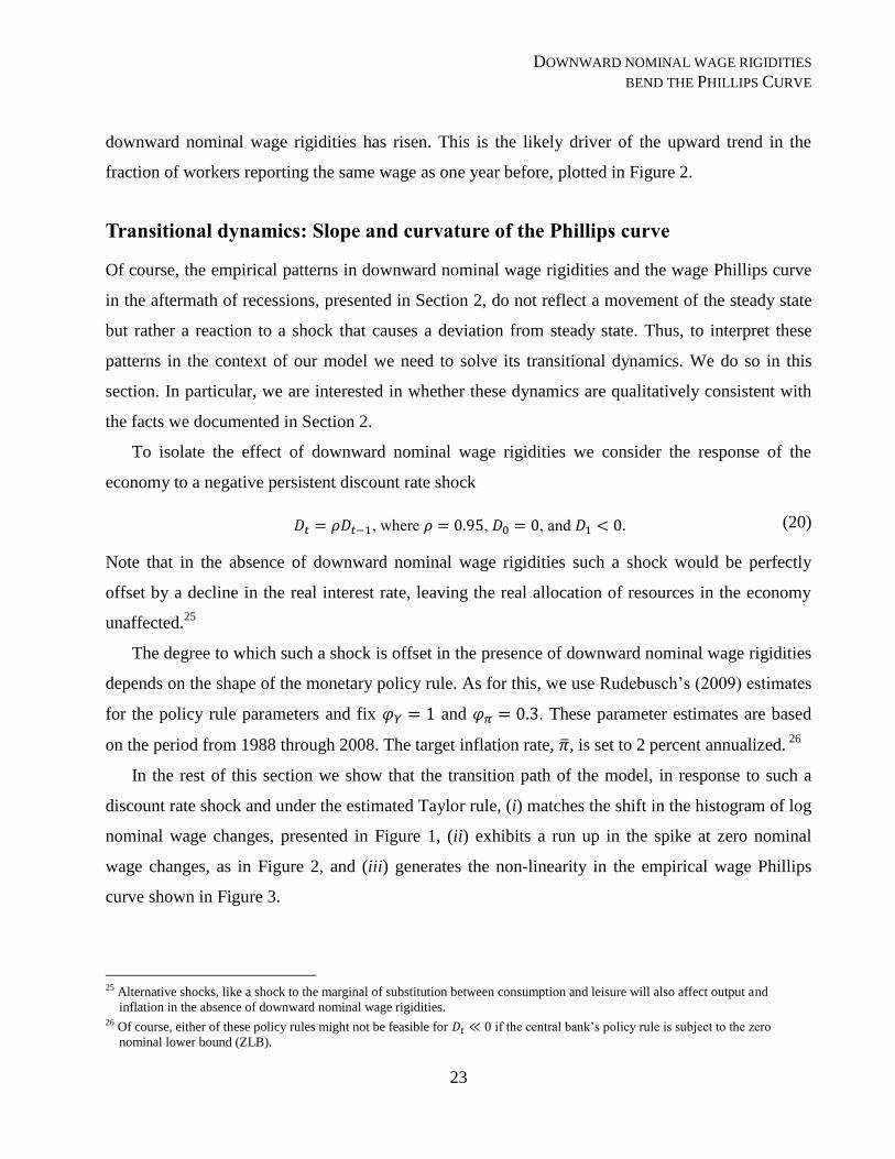
To isolate the effect of downward nominal wage rigidities we consider the response of the
economy to a negative persistent discount rate shock
, where , , and (20)
Note that in the absence of downward nominal wage rigidities such a shock would be perfectly
offset by a decline in the real interest rate, leaving the real allocation of resources in the economy
unaffected.25
The degree to which such a shock is offset in the presence of downward nominal wage rigidities
depends on the shape of the monetary policy rule. As for this, we use Rudebusch’s (2009) estimates
for the policy rule parameters and fix and . These parameter estimates are based
on the period from 1988 through 2008. The target inflation rate, , is set to 2 percent annualized. 26
In the rest of this section we show that the transition path of the model, in response to such a
discount rate shock and under the estimated Taylor rule, (i) matches the shift in the histogram of log
nominal wage changes, presented in Figure 1, (ii) exhibits a run up in the spike at zero nominal
wage changes, as in Figure 2, and (iii) generates the non-linearity in the empirical wage Phillips
curve shown in Figure 3.
25 Alternative shocks, like a shock to the marginal of substitution between consumption and leisure will also affect output and
inflation in the absence of downward nominal wage rigidities. 26 Of course, either of these policy rules might not be feasible for if the central bank’s policy rule is subject to the zero
nominal lower bound (ZLB).

DALY AND HOBIJN
24
To illustrate this, we solve for the model’s non-linear transitional dynamics keeping track of the
distribution of real wages along the equilibrium path. We do so by using the extended path method,
introduced by Fair and Taylor (1983).27
Our main example is the transitional dynamics after a large
discount rate shock equal to .28
Distortion of log nominal wage changes
Figure 9 shows the distribution of quarterly log wage changes right before the shock hits, at
when the economy is in steady state, as well as the distribution three years after the shock hits, at
. It is our model equivalent of Figure 1, interpreting 2006 as the steady state and 2011 as
after the shock.
Figure 9 illustrates that the model replicates three main features from the data. First, the spike at
zero nominal wage changes increases in response to the negative demand shock. This occurs
because the decline in inflation, in response to the shock, makes downward nominal wage rigidities
bind for more workers who are not able to reduce their wages. In addition, the likelihood of being
constrained by DNWR in the future increases for workers who are raising their wages, making them
temper their wage increases. These wage increases are further reduced by the negative demand
shock increasing the weight on the continuation value, ( ( )( )⁄ ), in equation
(13). This shock raises the effective marginal cost of pay increases even further and results in a
compression of wage increases similar to that shown in Figure 1. Note that this compression is fully
driven by the wage rigidities and is not due to a change in labor productivity, which is constant in
this simulation. Finally, just like in the data, there does not seem to be a large increase in the
fraction of workers with wage declines, though conditional on getting a reduction in the nominal
wage this decline is slightly larger after the shock than before.
27 Examples of other applications of this solution method are Hobijn, Ravenna, and Tambalotti (2006), who solve the transitional
dynamics of a model with nominal rigidities, and Carriga, Manuelli, and Peralta-Alva (2012) who consider the non-linear
transitional dynamics to a large shock that affects house prices. A more detailed description of how we implement the method can
be found in Appendix A. 28 One of the shortcomings of our model is that it requires a large discount rate shock to generate fluctuations in the unemployment
rate. This is a common problem in models of this type.

DOWNWARD NOMINAL WAGE RIGIDITIES
BEND THE PHILLIPS CURVE
25
Time-series path of spike at zero
Figure 10 confirms that the model also generates a persistent increase in the spike at zero wage
changes, just like in the data in Figure 2. The negative discount rate shock, in combination with the
monetary policy response, leads to a decline in the inflation rate, which results in an increase in the
fraction of workers who are stuck charging an undesirably high wage, making them sell fewer labor
services than they initially planned. As a consequence, the unemployment rate increases. Because of
the persistence of the shock these rigidities continue to bind even after the unemployment rate
begins to decline, just as in Figure 2.
Wage Phillips curve
The joint movement of inflation and unemployment along the transition path is depicted in Figure
11. The panels plot the short-run Phillips curves for different levels of rigidities (panel a), different
initial discount rate shocks (panel b), different inflation targets (panel c), and for the combination of
a discount rate and productivity shock (panel d).
Panel (a) compares our benchmark case of with the case of higher and lower
downward nominal wage rigidities. The plots confirm the intuition conveyed in Figure 5,
namely that higher DNWR lead to a higher sacrifice ratio and more bending of the Phillips curve.
We interpret this result as consistent with the idea that downward nominal wage rigidities are an
important factor that shapes the curvature of the empirical wage Phillips curve plotted in Figure 3.
According to our model, if downward nominal wage rigidities were not important, the type of
bending we have seen in the data following the last three recession and recovery periods would not
have occurred.
In panel (b) we plot the path for three different sizes of initial discount rate shocks,
{ }. The results show that the deeper the shock the longer the flat portion
of the Phillips curve persists. This implies that there can be long periods of stagnant wage growth,
even when unemployment is declining, especially after deep recessions. Again, the patterns
generated from our model are consistent with the data presented in Figure 3, and might help explain
why wage growth has been especially sluggish relative to decline in the unemployment rate in the
aftermath of the Great Recession.

DALY AND HOBIJN
26
Panel (c) considers how the impact of downward nominal wage rigidities varies with the
inflation target, , specifically target inflation of percent and percent, annualized. For
comparison purposes, the figure also includes the long-run Phillips curve for from Figure 6.
The first thing to note is that under the high target inflation rate of percent, downward
nominal wage rigidities are less binding and the short-run sacrifice ratio is smaller than under
percent. That is, the response to the initial shock under the high inflation target is more through
(wage) inflation and less through the unemployment rate than under the low inflation target. Under
percent the initial increase in the unemployment rate is 2.5 percentage points while wage
inflation decelerates by 6.5 percentage points. At percent this initial response is 2.7
percentage points on the unemployment rate and 2.5 percentage points on inflation respectively.
In addition to the response to the initial shock we can also compare the speed of the transition
back to steady state. If inflation greases the wheels then it might accelerate the pace with which the
economy returns to steady state in response to a shock. Surprisingly, the speeds of adjustment along
the two transitional paths plotted are very similar. Hence, our simulation results suggest that
increasing the target inflation rate, , to accelerate the pace of labor market adjustments might not
have a particularly large impact. Of course, this result is based on our particular model of downward
nominal wage rigidities and might change when these rigidities are included in a richer
macroeconomic framework.
Since recessions often are not solely the result of discount rate shocks, but often accompanied
by declines in labor productivity, the final panel of Figure 11, panel (d), plots the results for both a
productivity and a discount rate shock. Our productivity shock lowers labor productivity growth
from its historical annual average, 2.7 percent, to 0 at and then lets it come back gradually
according to
( ) ( ), where , , and (21)
The figure shows that if the economy is hit by a productivity shock alone, inflation rises and
unemployment increases. This is because the AD demand curve barely moves, while the SRAC
curve moves a lot, such that the economy moves along the AD curve producing both higher
inflation and higher unemployment (see Figure 5). In this sense, the productivity shock acts like a
classic supply shock in our model.
DOWNWARD NOMINAL WAGE RIGIDITIES
BEND THE PHILLIPS CURVE
27
Adding the demand shock to the experiment shows that recessions that coincide with slower
productivity growth produce an even flatter Phillips curve than ones where productivity growth is
unaffected. This can be seen by comparing the Phillips curve labeled discount rate shock to the one
labeled productivity and discount rate shock in panel (d). The additional flattening of the Phillips
curve owes to the fact that productivity growth, like inflation, greases the wheels of the labor
market. In periods of low productivity growth this additional grease is removed and the time period
over which wage growth remains stagnates while the unemployment rate fall is lengthened.
5. Conclusion
In this paper we made two main contributions. Our first contribution was empirical. We updated
and expanded existing micro data studies to document the existence of downward nominal wage
rigidities in the U.S. We also showed that these rigidities vary with the business cycle, but
asymmetrically. The prevalence of downward nominal wage rigidities spikes in recessions as
unemployment rises, but remains high well after unemployment begins to come down. Finally, we
highlighted the fact that this cyclical pattern of downward nominal wage rigidities coincides with
substantial curvature in the U.S. short-run Phillips curve.
Our second contribution was to understand the empirical patterns we described using a model of
monetary policy with downward nominal wage rigidities. Adding to previous research on the long-
run Phillips curve, we solved for the full non-linear transitional dynamics of the model in response
to demand and supply shocks, taking into account the evolution of the distribution of wages along
the equilibrium path. This focus on the joint cyclical path of unemployment and wage growth
following business cycle downturns is the key innovation of our paper.
The results highlight the importance of our approach. Our model was able to generate the key
patterns observed in the data, including the increase in downward nominal wage rigidities following
recessions and the subsequent bending of the short-run Phillips curve. Notably, we generate these
patterns in our model for parameter values under which downward nominal wage rigidities are
substantially less binding than empirical evidence suggests that they are in the U.S.
Overall, the model simulations showed that downward nominal wage rigidities bend the Phillips
curve in two ways. First, during recessions the rigidities become more binding and the labor market

DALY AND HOBIJN
28
adjustment disproportionately happens through the unemployment margin rather than through
wages. The higher the rigidities, the more this mechanism matters and the higher the short-run
sacrifice ratio between unemployment and inflation. Second, recessions result in substantial pent up
wage deflation. This leads to a simultaneous deceleration of wage inflation and a decline in the
unemployment rate during the ensuing recovery period. This bending of the Phillips curve is
especially pronounced in a low inflationary environment. We interpret our empirical work and
model simulations as evidence that downward nominal wage rigidities are an important force
shaping the dynamics of unemployment, wage growth, and inflation during and after the last three
U.S. recessions.
Fitting these complicated dynamics of wage growth and unemployment has turned out to be a
challenge for New-Keynesian models, like those analyzed in Galí, Smets, and Wouters (2011) and
Justiniano, Primiceri, and Tambalotti (2013). Though the simplified nature of our model, which
allowed us to solve for its non-linear transition path, only enabled us to qualitatively match the facts
on the distribution of nominal wage changes and the wage Phillips curve, our results suggest that
the inclusion of non-linear dynamics due to downward nominal wage rigidities with idiosyncratic
shocks in more elaborate macroeconomic models is a challenging but promising area for future
research.29
29 Like the models used to study the likelihood of hitting the ZLB in Chung et. al (2012), or the one used by Coibion et. al (2012).
Abbritti and Fahr (2013) is the state-of-the-art in this research area.

DOWNWARD NOMINAL WAGE RIGIDITIES
BEND THE PHILLIPS CURVE
29
References
Abbritti, Mirko, and Stephan Fahr (2013), “Downward Wage Rigidities and Business Cycle
Asymmetries,” Journal of Monetary Economics, 60, 871-886.
Akerlof, George A., William T. Dickens, and George L. Perry (1996), “The Macroeconomics of
Low Inflation,” Brookings Papers on Economic Activity, 1996-1, 1-52.
Altonji, Joseph G., and Paul J. Devereux (2000), “The extent and consequences of downward
nominal wage rigidity,” in (ed.) 19 (Research in Labor Economics, Volume 19), Emerald Group
Publishing Limited, 383-431.
Ball, Laurence (1994) “What Determines the Sacrifice Ratio?” in Monetary Policy, N. Gregory
Mankiw (ed.), University of Chicago Press.
Ball, Laurence, and N. Gregory Mankiw (1994), “Asymmetric Price Adjustment and Economic
Fluctuations,” The Economic Journal, 104, 247-261.
Barattieri, Alessandro, Susanto Basu, and Peter Gottschalk (2010) “Some Evidence on the
Importance of Sticky Wages,” NBER Working Papers 16130.
Benigno, Pierpaolo, and Luca Antonio Ricci (2011) “The Inflation-Output Trade-Off with
Downward Wage Rigidities,” American Economic Review, 101, 1436-1466.
Bewley, Truman F. (1995) “A Depressed Labor Market as Explained by Participants,” American
Economic Review, 85, 250-254.
Bewley, Truman F. (1999) Why Wages Don’t Fall During a Recession, Cambridge, MA: Harvard
University Press.
Bonin, Holger and Daniel Radowski (2011) “Downward nominal wage rigidity in services : direct
evidence from a firm survey,” Economics Letters, 106, 227-229.
Calvo, Guillermo A. (1983), “Staggered Prices in a Utility-Maximizing Framework,” Journal of
Monetary Economics, 12, 383-398.
Card, David, and Dean Hyslop (1997) “Does Inflation ‘Grease the Wheels of the Labor Market’?,”
in Reducing Inflation: Motivation and Strategy, Christina D. Romer and David H. Romer (eds),
71-122, National Bureau of Economic Research.
Carlsson, Mikael, and Andreas Westermark (2008) “Monetary Policy under Downward Nominal
Wage Rigidity,” BE Journal of Macroeconomics: Advances, 8, article 28.
Garriga, Carlos, Rodolfo E. Manuelli, and Adrian Peralta-Alva (2012) “A Model of Price Swings in
the Housing Market,” FRB St. Louis Working Paper 2012-022.
Chung, Hess, Jean-Philippe Laforte, David Reifschneider, and John C. Williams (2012) “Have We
Underestimated the Likelihood and Severity of Zero Lower Bound Events?” Journal of Money,
Credit and Banking, 44, S47-S82.
Coibion, Olivier, Yuriy Gorodnichenko, and Johannes Wieland (2012), “The Optimal Inflation Rate
in New Keynesian Models: Should Central Banks Raise Their Inflation Targets in Light of the
ZLB?” Review of Economic Studies, 79, 1371-1406.

DALY AND HOBIJN
30
Daly, Mary C., Bart Hobijn, and Brian T. Lucking (2012) “Why Has Wage Growth Stayed Strong?”
FRB SF Economic Letter 2012-10, April 2, 2012.
Daly, Mary C., Bart Hobijn, and Theodore S. Wiles (2011) “Dissecting Aggregate Real Wage
Fluctuations: Individual Wage Growth and the Composition Effect,” FRBSF Working Paper
2011-23.
Dixit, Avinash K., and Joseph E. Stiglitz (1977), “Monopolistic Competition and Optimum Product
Diversity,” The American Economic Review, 67, 297-308.
Dickens, William T. , Lorenz Goette, Erica L. Groshen, Steinar Holden, Julian Messina, Mark E.
Schweitzer, Jarkko Turunen, and Melanie E. Ward (2007) “How Wages Change: Micro
Evidence from the International Wage Flexibility Project,” Journal of Economic Perspectives,
21, 195-214.
Elsby, Michael W.L. (2009) “Evaluating the Economic Significance of Downward Nominal Wage
Rigidity,” Journal of Monetary Economics, 56, 154-169.
Erceg, Christopher J., Dale W. Henderson, and Andrew T. Levin (2000), “Optimal Monetary Policy
with Staggered Wage and Price Contracts,” Journal of Monetary Economics, 46, 281-313.
Fagan, Gabriel, and Julián Messina (2009), “Downward Wage Rigidity and Optimal Steady-State
Inflation,” ECB Working Paper No 1048.
Fair, Ray C., and John B. Taylor (1983), “Solution Maximum Likelihood Estimation of Dynamic
Nonlinear Rational Expectations,” Econometrica, 51, 1169-1185.
Fischer, Stanley, and Franco Modigliani (1978) “Towards an understanding of the real effects and
costs of inflation,” Review of World Economics (Weltwirtschaftliches Archiv), 114, 810-833.
Galí, Jordi (2011) “The Return of the Wage Phillips Curve,” Journal of the European Economic
Association, 9, 436-461.
Galí, Jordi, and Mark Gertler (1999) “Inflation dynamics: A structural econometric analysis,”
Journal of Monetary Economics, 44, 195–222.
Galí, Jordi, Frank R. Smets, Rafael Wouters (2011) “Unemployment in an Estimated New
Keynesian Model,” NBER Macroeconomics Annual 2011, 329-360.
Gottschalk, Peter (2005) “Downward Nominal-Wage Flexibility: Real or Measurement Error?,”
Review of Economics and Statistics, 87, 556-568.
Hobijn, Bart, Federico Ravenna, and Andrea Tambalotti (2006) “Menu Costs at Work: Restaurant
Prices and the Introduction of the Euro,” Quarterly Journal of Economics, 121, 1103-1131.
Holden, Steinar, and Fredrik Wulfsberg (2008) “Downward Nominal Wage Rigidity in the OECD,”
The B.E. Journal of Macroeconomics (Advances), 8(1), Article 15.
Justiniano, Alejandro, Giorgio E. Primiceri, and Andrea Tambalotti (2013) “Is There a Trade-Off
between Inflation and Output Stabilization?” American Economic Journal: Macroeconomics,
1-31.
Kahn, Shulamit (1997) “Evidence of Nominal Wage Stickiness from Microdata,” American
Economic Review, 87, 993-1008.
DOWNWARD NOMINAL WAGE RIGIDITIES
BEND THE PHILLIPS CURVE
31
Kahneman, Daniel, Jack L. Knetsch, and Richard Thaler (1986), “Fairness as a Constraint on Profit
Seeking: Entitlements in the Market,” American Economic Review, 76, 728-741.
Kim, Junil, and Francisco Ruge-Murcia (2009), “How Much Inflation is Necessary to Grease the
Wheels?” Journal of Monetary Economics, 56, 365-277.
Lebow, David A, Raven E. Saks, and Beth Anne Wilson (2003), “Downward Nominal Wage
Rigidity: Evidence from the Employment Cost Index,” B.E. Journal of Macroeconomics:
Advances, 3, issue 1.
Nekarda, Christopher J., and Valerie A. Ramey (2010) “The Cyclical Behavior of the Price-Cost
Markup,” mimeo.
Phillips, A. William (1958), “The Relationship between Unemployment and the Rate of Change of
Money Wages in the United Kingdom 1861-1957” Economica, 25, 283–299.
Rudebusch, Glenn D. (2009), “The Fed’s Monetary Policy Response to the Current Crisis,” FRBSF
Economic Letter 2009-17, May 22, 2009.
Samuelson, Paul A. and Robert M. Solow (1960) “Analytical Aspects of Anti-Inflation Policy,”
American Economic Review, 50, 177–194.
Taylor, John B. (1993), “Discretion versus Policy Rules in Practice,” Carnegie-Rochester
Conference Series on Public Policy, 39, pages 195-214 .
Tobin, James (1972), “Inflation and Unemployment,” American Economic Review, 62, 1-18.

DALY AND HOBIJN
32
Appendix A: Mathematical details
The household’s wage setting decision
The household maximizes
∑ ∑
{
∫
}
where (22)
It does so subject to the dynamic budget constraint
( ) ∫
(23)
and the labor demand function
(
)
(24)
Transformation of problem into real and detrended variables
Dividing both sides of the budget constraint, (23), by , yields the real detrended budget
constraint of the form
( )
( )( ) ∫
(25)
where ⁄ . In addition, substituting the equilibrium condition that ⁄ , we
obtain the real detrended version of the demand for labor of worker as
(
)
(26)
In addition, we can rewrite the household’s objective as
∑ ∑
{
∫
}
where (27)
Since the path of productivity, , is exogenous, it can be dropped from the objective function.
These are the transformed equations for which the optimality conditions are most easily solved and
most directly interpretable.
The first-order necessary conditions
The discrete-time Hamiltonian associated with this problem is

DOWNWARD NOMINAL WAGE RIGIDITIES
BEND THE PHILLIPS CURVE
33
∑ ∑
[
∫
{( )
( )( ) ∫
}]
(28)
Here is the discounted co-state variable.
Optimal consumption condition. The condition that determines the household’s optimal
consumption level, , is given by
∑ [
] (29)
Such that the marginal utility of consumption per dollar spent is equal to the co-state variable, in the
sense that
(30)
Optimal savings condition. The condition that determines the household’s optimal savings level, ,
is given by
∑ [
( )
( )( ) ] (31)
Rearranging the terms in this condition yields
( )
( )( ) (32)
Combining (30) and (32) gives the consumption Euler equation, (9), in the main text.
Wage-setting objective, equation (10)
We can isolate the part of the household’s Hamiltonian that involves the wage-setting of household
member . That part is
[∑ ∑
[
]
] (33)
Substituting in the result that ⁄ ⁄ , this objective can be simplified to
[∑ ∑
[
]
] [∑ ∑
( )
] (34)
This is equation (10) from the main text.

DALY AND HOBIJN
34
Wage setting under flexible wages, equation (12)
Under flexible wages, in each period household member chooses its real wage to maximize
( ). The associated first order condition is
( )
[ ( )
] (35)
Solving this condition for the real wage, , yields
(
)
(36)
This is equation (12) from the main text.
Properties of the optimal wage setting schedule, ( )
The Bellman equation associated with the dynamic wage-setting problem of the workers under
downward nominal wage rigidities is given by (13).
Workers that adjust their wage, are not subject to the DNWR constraint, and have the same set
the same wage ( ).
These workers choose their wage to solve
{ ( ) ( ( )( )⁄ )} (37)
The only respect with which workers differ is in terms of their productivity level. Hence, workers
with the same productivity level choose the same wage.
The wage-setting schedule, ( ), is such that ( ) ( ).
This is easiest seen by a transformation of variables. Instead of having the worker choose, , we
write its decision variable as ( ⁄ ) . This allows us to write
( )
(
( )( )
)
(38)
In addition, the transformed Bellman equation, (13), can be written as
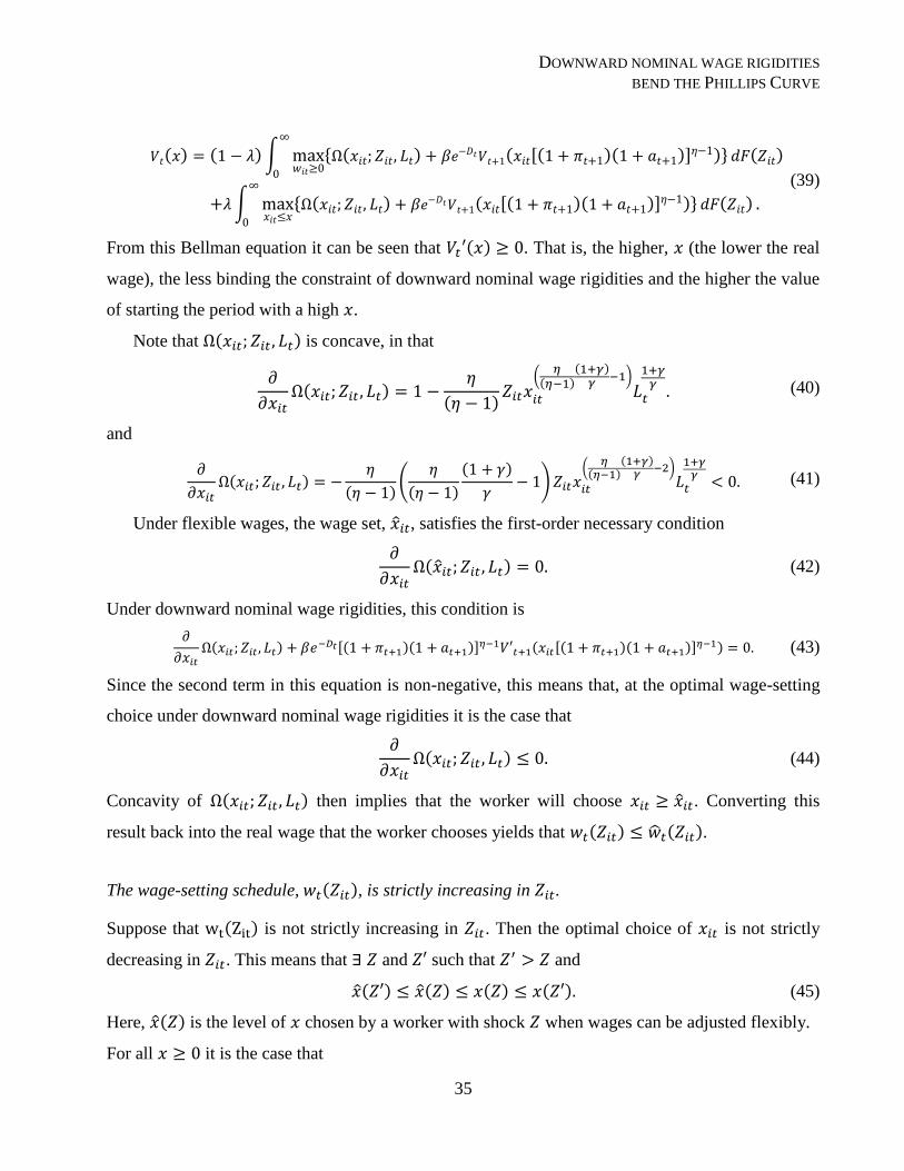
DOWNWARD NOMINAL WAGE RIGIDITIES
BEND THE PHILLIPS CURVE
35
( ) ( )∫
{ ( ) ( [( )( )]
)} ( )
∫
{ ( ) ( [( )( )] )} ( )
(39)
From this Bellman equation it can be seen that ( ) . That is, the higher, (the lower the real
wage), the less binding the constraint of downward nominal wage rigidities and the higher the value
of starting the period with a high .
Note that ( ) is concave, in that
( )
( )
(
( )( )
)
(40)
and
( )
( )(
( )
( )
)
(
( )( )
)
(41)
Under flexible wages, the wage set, , satisfies the first-order necessary condition
( ) (42)
Under downward nominal wage rigidities, this condition is
( ) [( )( )] ( [( )( )]
) (43)
Since the second term in this equation is non-negative, this means that, at the optimal wage-setting
choice under downward nominal wage rigidities it is the case that
( ) (44)
Concavity of ( ) then implies that the worker will choose . Converting this
result back into the real wage that the worker chooses yields that ( ) ( ).
The wage-setting schedule, ( ), is strictly increasing in .
Suppose that ( ) is not strictly increasing in . Then the optimal choice of is not strictly
decreasing in . This means that and such that and
( ) ( ) ( ) ( ) (45)
Here, ( ) is the level of chosen by a worker with shock when wages can be adjusted flexibly.
For all it is the case that

DALY AND HOBIJN
36
( ( ) ) ( ( )[( )( )] )
( ) ( [( )( )] )
(46)
and
( ( ) ) ( ( )[( )( )] )
( ) ( [( )( )] )
(47)
The last equation implies that
( ) ( )
[ ( ( )[( )( )] ) ( ( )[( )( )]
)]
[ ( )(
( )
( )
) ( )
(
( )( )
)]
(48)
Since , this thus implies that
( ) ( )
[ ( ( )[( )( )] ) ( ( )[( )( )]
)]
[ ( )
(
( )( )
) ( )
(
( )( )
)]
(49)
Rearranging terms, this means that
( ( ) ) ( ( )[( )( )] )
( ( ) ) ( ( )[( )( )] )
(50)
But this implies that ( ) cannot be the optimal choice for a worker with shock . Hence, the
optimal choice of is strictly decreasing in . Consequently, ( ) is strictly increasing in .
Workers that are subject to DNWR and for whom ( ) will keep wage fixed.
The easiest way to show this is to show that if DNWR are binding at , which is the case when
( ) , then they are binding at all . Suppose not, then
( ) ( [( )( )] )
( ) ( [( )( )] )
(51)
while there and such that
( ) ( [( )( )]
)
( ) ( [( )( )] )
(52)
But, using the similar argument as in equations (48) and (49) these two equations can be shown to
contradict each other. Thus, if DNWR are binding at , then they are binding for all . Hence,
any worker subject to DNWR at a wage ( ) will keep their wage fixed.

DOWNWARD NOMINAL WAGE RIGIDITIES
BEND THE PHILLIPS CURVE
37
The log normal distribution
For the disutility from working shock, , we assume that it is drawn from a log-Normal distribution,
such that (
). Throughout, we denote the standard Normal distribution function by
( ) and the corresponding density by ( ).
For our derivations, we extensively use the properties of the log-Normal distribution that make
make expectations of various exponentials of the random variable easily tractable. First note that we
choose the mean
such that
( )
(53)
Hence, the average productivity level across firms equals one.
Moreover,
( )
( )
(54)
and, consequently, we find that
[ ( )]
( )
(55)
The final property that we use is that of the truncated log normal. In particular, we apply that for
( ) ∫
( ) ( ( ) ( )) ( )
(56)
where
(
) ⁄ and (
) ⁄ (57)
Equilibrium
Dynamics of density function of real wages
Differentiation of (17) yields the recursive equation for the density function
( ) ( ) ( ) ( ( ))
( ( )( )) ( ) ( ( ))
( ) ( ( )( )) ( ( ))
(58)

DALY AND HOBIJN
38
Each of the lines in this expression corresponds to the respective type of worker discussed in the
main text.
Equilibrium under flexible wages, , equation (15)
When wages can be adjusted flexibly they are set such that
(
)
(59)
The corresponding level of labor demand is given by
(
)
(
)
(
)
( )
(60)
Such that
[∫
]
(
)
( )
[∫ (
)
( )
]
(61)
Solving this for ⁄ , this yields
(
)
[∫ (
)
( )
]
( )( )
(62)
This expression simplifies to (15).
Equilibrium under downwardly rigid wages, , equation (18)
In equilibrium the real wage equals one. This means that
[∫ (
)
]
[∫ (
)
] [∫ (
)
(
)
]
(
)
( )
( )( )
[∫ (
)
( )
(
)
]
(63)
We divide the integral in this equation into three parts, corresponding to (i) workers that are not
subject to the DNWR constraint, (ii) workers that are subject to it but for whom it is not binding,
and (iii) workers for whom the constraint is binding. Doing so, we can write

DOWNWARD NOMINAL WAGE RIGIDITIES
BEND THE PHILLIPS CURVE
39
(
)
( )
( )( )
{( )∫ (
)
( )
( ( )
( ))
( )
∫ (
)
( )
( ( )( )( )) ( ( )
( ))
( )
∫ [∫ ( )( ) ( ( )( )) ( ( )
)
( )
] ( )
}
(64)
When we define
{( )∫ (
)
( )
( ( )
( ))
( )
∫ (
)
( )
( ( )( )( )) ( ( )
( ))
( )
∫ (
)
( )
[∫ ( )( ) ( ( )( )) ( ( )
)
( )
] ( )
}
( )
(65)
Then the equilibrium condition can be written as
(
)
( )
(
)
( )
( )( )
(66)
Solving this with respect to ⁄ yields that
(
)
(
)
(67)
This is equation (18) in the main text.
Numerical method
Approximation of the distribution and density functions of real wages, ( ) and ( )
Throughout, we use polynomial approximations for the value function ( ) and the wage-setting
schedule, ( ) and ( ). We truncated the log-normal distribution of at and , such that
( ) ( ) . Truncating the distribution of the disutility shocks means that, at a non-
negative target inflation rate, , the support of the steady-state real wage distribution is bounded.
This, in turn, means that the support of the real wage distribution is bounded at any point along the

DALY AND HOBIJN
40
transition path. We then use Piecewise Cubic Hermite Interpolating Polynomials to approximate
( ) on this bounded support. Since these polynomials are differentiable, they also allow us to
calculate ( )
Steady state solution
In the steady state the inflation rate equals the inflation target, . The steady state is solved by
iterating over the following steps: (i) For a given level of output , iterate over the Bellman
equation until convergence. This gives the wage-setting schedule, ( ) and ( ). (ii) Given the
wage-setting schedule, iterate over the recursive equation for the distribution function of real wages
( ) to obtain the corresponding real wage distribution. (iii) Give the wage-setting schedule and
the distribution of real wages, solve for the level of that equates the real wage to one using the
equilibrium condition under downwardly rigid nominal wages, i.e. (18).
Transition path
The application of calculating the transition path using the extended path method involves the
following steps. The path is calculated for under the assumption that the economy is in
steady state at time and at time . We start off assuming the economy is in steady state
along the whole path, except that the discount rate shock is not zero along that path. (i) In the first
step we use a backward recursion for the policy rule to obtain the nominal interest rate and inflation
rate that the central bank would set in response to the path of { } . (ii) For the path of the
inflation rate { } we then solve the path of the optimal wage setting schedule { ( )}
through backward recursion using the assumption that the economy is in steady state for . (iii)
Given the path of { ( )} we then use forward recursion to solve the path of { ( )}
. (iv)
Given the paths of { ( )} and { ( )}
we then calculate the implied path of { } . We
iterate over steps (i) through (iv) until convergence.
DOWNWARD NOMINAL WAGE RIGIDITIES
BEND THE PHILLIPS CURVE
41
Appendix B: Data details
Current Population Survey (CPS)
The CPS is a monthly survey conducted by the Bureau of Labor Statistics. CPS participants stay
with the survey for 18 months and over the course of that period are asked to report on earnings
twice, once towards the beginning of their time and once towards the end-with the intervening time
span equaling 12 months. Since we are interested in wage changes among all workers in the
economy, our sample includes both workers who remain with their employer and those who change
jobs during the period over which they report their earnings. Similarly, we include both salaried
workers and workers paid at an hourly rate. For those paid at an hourly rate we use reported hourly
earnings; for salaried workers we impute an hourly wage by dividing weekly earnings by hours
worked per week. Nominal wage changes are computed for each worker as the difference in their
reported log wages. Our final CPS dataset contains monthly information on the distribution of
nominal wage changes for a representative sample of U.S. workers for the period from January
1980 to February 2013. For more details regarding using the CPS for this purpose see Daly, Hobijn
and Wiles (2011).
Matching individuals across CPS interviews in different months
Our CPS dataset is constructed using the outgoing CPS monthly files from the BLS. We match
individuals across different months using the matching algorithm detailed in Daly, Hobijn, and
Wiles (2011). Specifically, individuals must match on age (+3 or -1 years between subsequent
interviews), race, household ID, and line number. The Census scrambled household identifiers in
July 1985 and June 1995, so we cannot match individuals one year forward from this date. This
means that our dataset contains no wage change data from July 1985 to June 1986 and from June
1995 to May 1996. We use all 8 interview months (IMs) in order to match individuals and to
determine if they are job stayers, but our final dataset contains only the outgoing rotation groups
(IM 4 and IM 8) which are the only rotation groups with earnings information.

DALY AND HOBIJN
42
Constructing wage variables
When collecting a worker’s earnings data, the BLS ascertains if the worker in question is paid at an
hourly rate. If so, the worker’s hourly rate of pay excluding overtime, tips, and commissions is
recorded. We use this measure of earnings when available. Otherwise, we divide usual weekly
earnings by usual hours worked per week to create an imputed hourly rate of pay. The BLS collects
usual weekly earnings data by asking respondents to report their earnings in the easiest way, and
then converting to a weekly rate of pay. Workers that are paid at an hourly rate and do not make
more than the binding minimum wage in their state of residence (in either IM 4 or IM 8) are
dropped from the sample. We also drop workers with any top-coded earnings data and restrict our
analysis to workers age 16 and older. Our final dataset consists of 12-month rolling panels of hourly
wage data from January 1980 to February 2013. Wage changes are calculated as the difference in
the log of hourly wages from one year ago. In other words, in our dataset a wage change of 0.1 in
January 2013 means that the log of a worker’s reported or imputed hourly wage in January 2013
was 0.1 greater than the log of his or her hourly wage in January 2012.
Wage composite for wage Phillips curve
The four wage series we use to construct our composite index of wage growth are Compensation
per hour (CPH), the Employment Cost Index (ECI), Median usual Weekly Earnings (MWE), and
Average Hourly Earnings (AHE). Galí (2011) plots separate wage Phillips curves for CPH and
AHE. Combining the four most commonly used wage measures follows the idea of Justiniano,
Primiceri, and Tambalotti (2013) who include separate measurement equations for CPH and AHE
in the state-space representation of their model and estimate the time-series as wages as the,
structurally identified, factor that drives both. We add the ECI and MWE to use the additional
information that they contain. Figure B1 plots the four series and their first principle component
which we use as our composite measure of nominal wage growth.

DOWNWARD NOMINAL WAGE RIGIDITIES
BEND THE PHILLIPS CURVE
43
Table 1. Parameter values for benchmark numerical simulation
Parameter Value Interpretation Reference
0.5 Frisch labor supply elasticity Benigno and Ricci (2011)
2.5 Labor demand elasticity for
labor services of a worker Benigno and Ricci (2011)
0.9 Share of workers subject to
DNWR in each quarter
Chosen conservatively to generate smaller
spike at 4-quarter zero wage changes than
in data. See Figure 8.
0.25
Standard deviation of idiosyn-
chratic disutility of working
shock
Chosen to get a steady-state unemployment
rate of 5 percent.
0.3 Taylor-rule parameter on
inflation Rudebusch (2009)
1 Taylor-rule parameter on the
output gap Rudebusch (2009)
0.9950 Discount factor 2 percent discounting annually
0.0050 Target inflation rate 2 percent annualized target inflation
0.0066 Trend productivity growth 2.7 percent average annualized labor
productivity growth over 2001-2007 (BLS)
Figure 1. Distribution of 12-month log wage changes in 2006 and 2011.
0
2
4
6
8
10
12
14
16
-20 -10 0 10 20
Source: Current Population Survey and authors' calculations.
Frequency
2011
2006

DALY AND HOBIJN
44
Figure 2. Fraction of workers reporting the same wage as one year prior
and the unemployment rate.
Figure 3. The U.S. wage Phillips curve: 1986-2012.
6
8
10
12
14
16
18
2
4
6
8
10
12
14
1986 1989 1992 1995 1998 2001 2004 2007 2010 2013Source: Bureau of Labor Statistics and Current Population Survey. 12-month centered MA of rate of wage change.
Percent Percent
Rate of no wage change (right axis)
Unemployment rate (left axis)
-2
-1
0
1
2
3
-2 -1 0 1 2 3 4 5
Source: Bureau of Labor Statistics and authors' calculations
Unemployment gap
Nominal wage growth gap (4Q)
1990 recession
2001 recession
2007 recession

DOWNWARD NOMINAL WAGE RIGIDITIES
BEND THE PHILLIPS CURVE
45
Figure 4. Different groups of workers that determine dynamics of distribution of real wages.
w
Z
0
z (w’)t
w’
z (w)t
A
B
C

DALY AND HOBIJN
46
Figure 5. How shifts in aggregate demand and aggregate supply bend the Phillips Curve.
AD
AD’
SRAS SRAS’
p
u
2%
5%
AD
AD’
SRAS SRAS’
p
u
2%
5%
(a) low rigidities
(b) high rigidities

DOWNWARD NOMINAL WAGE RIGIDITIES
BEND THE PHILLIPS CURVE
47
Figure 6. Long-run Phillips curve for different parameter combinations.
Figure 7. Steady-state distribution of quarterly under flexible wages and DNWR.
0
1
2
3
4
5
6
7
8
9
10
0 1 2 3 4 5 6 7 8Unemployment rate
Target inflation rate (annualized)
4 8
,
5
= 0.9 = 0.99
0
10
20
30
40
50
60
0
1
2
3
4
5
6
7
8
9
10
-20 -15 -10 -5 0 5 10 15 20( )
Frequency (percent) Spike at zero (percent)
Flexible
DNWR
DNWR Spike
(right axis)
5

DALY AND HOBIJN
48
Figure 8. Fraction of workers with no wage change over 4 quarters for different values of and .
Figure 9. Distribution of quarterly in steady state and after shock at .
0
1
2
3
4
5
6
7
8
9
10
0 2 4 6 8 10Target inflation rate (annualized)
Percent
= 0.4
= 0.8
= 0.8,
= 0.99
= 0.9
5
0
10
20
30
40
50
60
70
80
0
1
2
3
4
5
6
7
8
9
10
-10 -9 -8 -7 -6 -5 -4 -3 -2 -1 0 1 2 3 4 5 6 7 8 9 10
Frequency (percent) Spike at zero (percent)
Steady State
Spike at 0
in steady state
(right axis)
After shock at
Spike at 0
after shock at
(right axis)

DOWNWARD NOMINAL WAGE RIGIDITIES
BEND THE PHILLIPS CURVE
49
Figure 10. Paths unemployment rate, and spike in zero 4-quarter wage changes.
4
4.5
5
5.5
6
6.5
7
7.5
8
0 1 2 3 4 5 6 7 8 9 101112131415161718192021222324252627282930
For , , and , where
Quarters since demand shock,
Percent
Unemployment rate
Fraction of workers
with no wage change
over 4 quarters

DALY AND HOBIJN
50
Figure 11. Four examples of the bending of the Phillips Curve.
-2
-1
0
1
2
3
4.5 5 5.5 6 6.5 7 7.5 8
Panel (a): Different levels of rigidities
Unemployment rate
Wage inflation (annualized)
= 0.80
= 0.90
= 0.99
,
-2
-1
0
1
2
3
4.5 5 5.5 6 6.5 7 7.5 8
Panel (b): Three different discount rate shocks
Unemployment rate
Wage inflation (annualized)
LRPC
-2
-1
0
1
2
3
4
5
6
7
8
9
10
11
2 3 4 5 6 7 8
Panel (c): Different inflation targets
Unemployment rate
Wage inflation (annualized)
,
(annualized)
(annualized)
LRPC
-2
-1
0
1
2
3
4
4.5 5 5.5 6 6.5 7 7.5 8 8.5
Panel (d): Discount rate, productivity, and both shocks
Unemployment rate
Wage inflation (annualized)
Discount rate shock
Productivity and discount rate shocks
Productivity shock

DOWNWARD NOMINAL WAGE RIGIDITIES
BEND THE PHILLIPS CURVE
51
Figure B1. Four measures of nominal wage growth and their first principle component.
0
1
2
3
4
5
6
7
8
9
1986 1991 1996 2001 2006 2011
CPH
ECI
MWE
AHE
Principal Component
Source: Bureau of Labor Statistics and authors' calculations
4-quarter percent changePercent


